DELFT UNIVERSITY OF TECHNOLOGY

REPORT 03-03

A Mass-Conserving Level-Set (MCLS) Method for Modelingof Multi-Phase Flows

S.P. van der Pijl, A. Segal, C. Vuik

ISSN 1389-6520

Reports of the Department of Applied Mathematical Analysis

Delft 2003

Copyright 2000 by Department of Applied Mathematical Analysis, Delft, The Netherlands.

No part of the Journal may be reproduced, stored in a retrieval system, or transmitted, in

any form or by any means, electronic, mechanical, photocopying, recording, or otherwise,

without the prior written permission from Department of Applied Mathematical Analysis,

Delft University of Technology, The Netherlands.

A Mass-Conserving Level-Set (MCLS) Method

for Modeling of Multi-Phase Flows

S.P. van der Pijl∗ A. Segal C. Vuik

February 25, 2003

Abstract

The Mass-Conserving Level-Set (MCLS) method is proposed to modelmulti-phase flows. The aim is to model high density-ratio flows with com-plex interface topologies, such as mixtures of bubbles and droplets. As-pects which are taken into account are: a sharp front (density changesrapidly), arbitrary shaped interfaces, surface tension, buoyancy and co-alescence of drops/bubbles. Attention is paid to mass-conservation andintegrity of the interface.

A survey of available computational methods is performed in [1]. Theproposed computational method is a combination of Level-Set and Volume-of-Fluid methods. The flow is computed with a pressure correction methodwith a Marker-and-Cell layout. Interface conditions are satisfied by meansof the continuous surface force/stress (CSF/CSS) methodology and theGhostFluid method for incompressible flows.

The Level-Set method is an elegant method. The major disadvan-tage is that it is not rigorously mass-conserving. This means that ad-ditional effort is necessary to conserve mass. The MCLS method intro-duces a Volume-of-Fluid function, which is advected without the neces-sity to reconstruct the interface. There is a strong relationship betweenthe Volume-of-Fluid function and the Level-Set function. In the spiritof the Level-Set methodology, the advection of the VOF-function is, un-like other VOF methods, purely implicit at every time. This makes themethod straightforward to apply to arbitrarily shaped interfaces, whichmay collide and break up.

1 Introduction

Multi-phase flows occur commonly in engineering fluid mechanics. In this workmodeling of incompressible two-phase flows is considered. The present researchaims to model high density-ratio flows with complex interface topologies, typ-ically air/water flows. A sharp front exists between the phases, where fluid

∗Research granted by NWO.

1

density and viscosity change rapidly. This front is modeled as an interface be-tween the phases where fluid properties are discontinuous. The interface is amoving (internal) boundary. Also, surface tension forces act on the interface. Anumerical method has to take this into account as well as to be able to handlearbitrarily shaped interfaces which may collide and break up.

Various methods have been put forward to treat multi-phase flows. A clas-sification is given in [1]. Most generally speaking, the interface representationcan be explicit (‘moving, boundary conforming mesh’) or implicit (‘fixed mesh’)or a combination of both. Purely moving, boundary-conforming meshes will becumbersome, since the objective is to simulate arbitrarily shaped interfaces. Itis therefore not very suited to apply to this work.

A combination of fixed and moving mesh methods include the hybrid front-tracking/front-capturing method ([2–6]) and the closely related immersed bound-ary method ([7–10]). Although the interface is tracked by an interface grid, theflow is solved on a stationary grid. The interface conditions are satisfied byregularizing (smoothing) the interface discontinuities and interpolating inter-face forces from the interface grid to the stationary grid. For this purpose, theinterface forces are transformed into volume forces and distributed over certainmesh widths. This is sometimes referred to as the continuous surface force(CSF) or continuous surface stress (CSS) approach ([11]). As far as solving theflow field is concerned, the interface position is not prescribed explicitly. Theinterface grid on the other hand is advected by interpolating the velocity fieldfrom the stationary grid to the interface grid. A drawback of the method mightbe that the interface grid can get hard to evaluate, especially when interfacescollide or break up. Furthermore, interpolating from the interface grid to thestationary grid is carried out by smearing of interface forces and discontinu-ities over certain mesh widths. This can introduce so-called parasitic currents([6]) which are unphysical regions of recirculated fluid near the interface. Inthe cut-cell approach ([12–17]) on the other hand, the interface conditions aresatisfied without smoothing of the interface. The control volumes of the sta-tionary grid are readjusted near the interface, so that it is locally boundaryconforming. It has been successfully applied to fluid-solid interfaces, where avelocity is prescribed on the interface. However, in case of two-phase flows, theinterface separates two fluids and the interface conditions express continuity ofmass and momentum over the interface. The cut-cell approach is extended tohandle fluid-fluid interfaces in [18] by iteratively modifying the interface shape,such that the interface conditions are satisfied. Since control volumes have tobe readjusted, the cut-cell method requires a large amount of logic decisions. Atfirst sight the method seems to be cumbersome to apply in three-dimensionalspace. Also, the iterative procedure is not trivial.

The combined implicit/explicit methods are sometimes referred to as ‘front’-or ‘surface tracking’ methods. The interface grid which is needed to track themoving boundary will be difficult to evaluate when the interface has arbitraryshape and topology. Instead, for the current research the implicit methods havebeen selected to represent the interface. These methods are also called ‘volumetracking’ methods. The interface is implicitly defined by marking it by particles

2

or by a function.With the Marker-and-Cell (MAC) method ([19]), one of the two phases

is indicated by marker particles. With the Surface Marker and Micro Cell(SMMC) method ([20]) the interface itself is marked by particles. The particlesare advected by the flow field. For both methods it is hard to compute interfacequantities like the normal vector and curvature in order to model surface tensionforces, since the connectivity of particles is unknown (otherwise these would befront-tracking methods).

The two volume-tracking methods that are most suitable for the currentresearch are the Volume-of-Fluid (VOF) method and the Level-Set method. Forboth methods a marker function is used to define the interface. In case ofthe Volume-of-Fluid method, a marker function, say Ψ, indicates the fractionalvolume of a certain fluid, say fluid ‘1’, in a computational cell. It can be seen asthe concentration of the marker particles of the MAC-method, when the numberof particles goes to infinity. Hence Ψ is defined in a grid cell Ω by

Ψ =1

vol(Ω)

∫

Ω

χ dΩ, (1)

where χ is the characteristic function

χ =

1 in fluid ‘1’,0 outside fluid ‘1’.

(2)

The value of Ψ will be 0 or 1 in cells without the interface and 0 ≤ Ψ ≤ 1 in cellscontaining the interface. In other words, the value of Ψ changes rapidly acrossthe interface. This causes difficulties in advecting Ψ. The step-like behaviorof Ψ will be lost by the straightforward application of a numerical scheme.Hence the interface will get ill defined. Volume-of-fluid methods can suffer from‘flotsam and jetsam’, which are the small remnants of mixed-fluid zones ([21]).Besides that, the step-like behavior of the marker function makes computinginterface derivatives (normals, curvature) elaborate. The major advantage ofVOF methods is that mass is rigorously conserved, provided the discretizationis conservative.

Advecting Ψ is not a straightforward task. This can either be performedalgebraically or geometrically. Algebraic methods try to discretize the advectionequation for the marker function Ψ by incorporating the step-like behavior ofΨ. Examples of such approaches are: Constrained Interpolation Profile ([22–24]) and Flux-Corrected Transport (FCT) (([25, 26]). Geometric methods onthe other hand first reconstruct the interface from Ψ, after which it is advected.Geometric VOF methods differ in the accuracy of the interface reconstruction.With Simple Line Calculation (SLIC) the interface is assumed to be piecewisetangential to a coordinate direction ([21]). In case of the donor-acceptor (SOLA-VOF) method the interface is stair-stepped ([27, 28]). And with the PiecewiseLinear Interface Calculation (PLIC) method the interface is piecewise linear([26, 29–33]). Reconstruction of the interface will be increasingly difficult if the

3

discrete interface representation is more accurate. This is a drawback especiallyof the PLIC method, which on the other hand is the most accurate method.

An alternative to the Volume-of-Fluid methods is the Level-Set method ([34–37]). The interface is now defined by the zero level-set of the marker function,say Φ:

Φ

< 0 outside fluid ‘1’,= 0 at the interface,> 0 inside fluid ‘1’.

(3)

The function Φ is chosen such that it is smooth near the interface. This easesthe computation of interface derivatives. Also, methods available from hyper-bolic conservation laws can be used to advect the interface. The interface is(implicitly) advected by advecting Φ as if it were a material constant:

∂Φ

∂t+ u · ∇Φ = 0. (4)

Although this makes the Level-Set method an elegant method, the major disad-vantage is that it is not rigorously mass-conserving. This means that additionaleffort is necessary to conserve mass, or at least to improve mass conservation.One approach would be to approximate Eqn. (4) more accurately by higher or-der schemes or by grid refinement. In [38–40] higher order ENO discretizationof Eqn. (4) is adopted and in [41–43] the grid is refined adaptively near theinterfaces.

The interface forces and discontinuities are often smeared out over certainmesh widths in a CSS/CSF way. To keep the smeared-out interface thicknessconstant in the course of time, it is necessary that the Level-Set function is a so-called distance function at all time instants. This is achieved by re-initializationin [44]. However, when the interface is advected through the flow field, theviolation of mass-conservation is increased due to re-initialization. Therefore,improved re-initialization is carried out in [38–40].

Mass-conservation is improved due to all aforementioned efforts, but neverexactly satisfied. In [45] the mass-conservation properery of the Level-Setmethod is improved by adding passively advected marker particles. These par-ticles are used near the interface. It can be seen as a coupling of the Level-Setand Marker-and-Cell methods. It is required to keep track of the particles andto redistribute the particles, which increases the amount of bookkeeping. Thevelocity field has to be interpolated at the particle positions. Furthermore,the interface has to be reconstructed from the particles. This might not be astraightforward task.

The Coupled Level-Set Volume-of-Fluid (CLSVOF) method ([46]) is a cou-pling of the Level-Set method with the Volume-of-Fluid PLIC method. Besidesthe advection of the Level-Set function Φ also the Volume-of-Fluid functionΨ is advected. However, there is no straightforward relationship between theLevel-Set function and the Volume-of-Fluid function; both advections are inde-pendent. After each update of Φ and Ψ, coupling of both functions takes place.This coupling is not easily achieved. Since the PLIC approach is employed, a

4

drawback of this method might be that besides mass-conservation, also the elab-orateness of the VOF methods is imported. The mass-conservation propertiesare shown to be comparable to VOF methods.

This work also combines the Level-Set method with the Volume-of-Fluidmethod. A VOF-function Ψ is introduced, which is advected without the ne-cessity to reconstruct the interface. There exists a strong relationship betweenthe Volume-of-Fluid function and the Level-Set function Φ. In the spirit ofthe Level-Set methodology, the advection of the VOF-function is, unlike PLICand consequently CLSVOF, purely implicit at all time. This makes the methodstraightforward to apply to arbitrarily shaped interfaces, which may collide andbreak up.

2 Governing Equations

Consider two fluids ‘0’, and ‘1’ in domain Ω ∈ IR2 which are separated by aninterface S. Both fluids are assumed to be incompressible, i.e.:

∇ · u = 0, (5)

where u = (u, v)t is the velocity vector and u and v are the velocities in x- and y-direction respectively. The flow is governed by the incompressible Navier-Stokesequations:

∂ρu

∂t+ ∇ · (ρuu) = −∇p + ∇ · µ

(∇u + ∇ut

)+ ρg, (6)

where ρ, p, µ and g are the density, pressure, viscosity and gravity vectorrespectively. With Eqn. (5), this is rewritten as

∂u

∂t+ u · ∇u = −

1

ρ∇p +

1

ρ∇ · µ

(∇u + ∇ut

)+ g, (7)

The density and viscosity are constant within each fluid. Using the Level-Setfunction Φ as defined in Eqn. (3), these can be expressed as

ρ = ρ0 + (ρ1 − ρ0)H(Φ) (8)

andµ = µ0 + (µ1 − µ0)H(Φ), (9)

where the subscript indicates the corresponding fluid and H is the Heavisidestep function.

2.1 Interface conditions

The interface conditions express continuity of mass and momentum at the in-terface:

[u] = 0[pn− n · µ (∇u + ∇ut)] = σκn,

(10)

5

where the brackets denote jumps across the interface, n is a normal vector atthe interface, σ is the surface tension coefficient and κ is the curvature of theinterface. Clearly, the velocity u is continuous at the interface. Concerningthe derivatives of the velocity, if s is parallel to the interface, un = n · u andus = s · u, in [47, 48] it is shown that in general

[∂un

∂n

]= 0,

[∂un

∂s

]= 0

[∂us

∂n

]= −[µ]

∂un

∂s,

[∂us

∂s

]= 0.

(11)

Note that if the viscosity µ is continuous at the interface, Eqn. (11) shows thatthe derivatives of the velocity components are continuous too. The viscosity isforced to be continuous by smoothing Expression 9:

µ = µ0 + (µ1 − µ0)Hα(Φ), (12)

where Hα is the smoothed (or regularized) Heaviside step function

Hα(x) =

0 x < −α12

(1 + sin( x

α12π))

|x| ≤ α1 x > α

(13)

and α is a parameter proportional to the mesh width. Here α is chosen as (fol-lowing [44]) α = 3

2h, where h is the mesh width. According to [38], the viscosityis then smoothed over three mesh widths, provided |∇Φ| = 1. Furthermore, ifthe Level-Set function Φ is a distance function, i.e. |∇Φ| = 1, then

µ = µ0 + (µ1 − µ0)Hα(Φ). (14)

Note that only the viscosity is smoothed, not the density ρ. Instead of takinginto account the pressure-jump at the interface due to the surface tension forces,the continuous surface force/stress (CSF,CSS, [11]) methodology is adopted.

3 Computational Approach

The Navier-Stokes equations are solved by the pressure-correction method ([49]).The unknowns are stored in a Marker-and-Cell layout ([19]). For the interfacerepresentation a combination of the Level-Set and Volume-of-Fluid methodolo-gies are adopted. The interface conditions are satisfied by means of the contin-uous surface force/stress (CSF/CSS) methodology and the GhostFluid methodfor incompressible flow ([47, 50]).

3.1 Pressure Correction

The Navier-Stokes equations (Eqn. (7)) are discretized in a finite differencefashion by employing the pressure correction methodology. The unknowns u, v

6

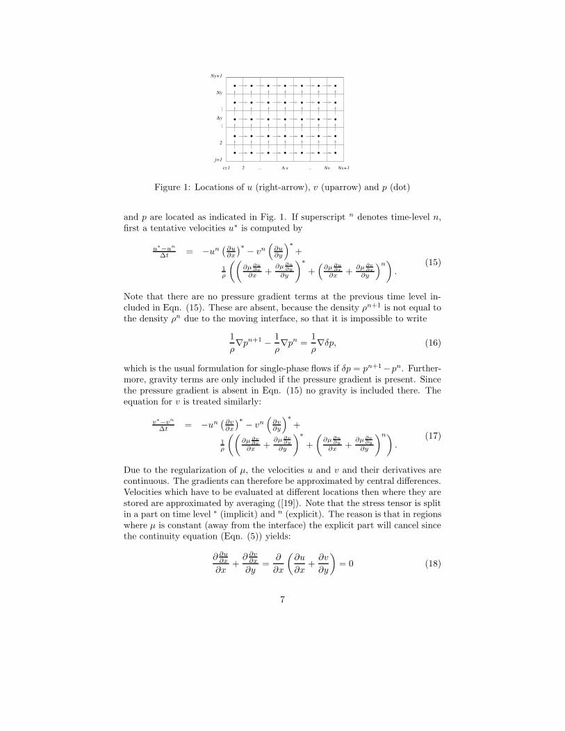
i=1 ... ... Nx+12

j=1

2

∆ x

y∆

Ny

Ny+1

Nx

......

Figure 1: Locations of u (right-arrow), v (uparrow) and p (dot)

and p are located as indicated in Fig. 1. If superscript n denotes time-level n,first a tentative velocities u∗ is computed by

u∗−un

∆t= −un

(∂u∂x

)∗− vn

(∂u∂y

)∗+

1ρ

((∂µ ∂u

∂x

∂x+

∂µ ∂u∂y

∂y

)∗

+(

∂µ ∂u∂x

∂x+

∂µ ∂v∂x

∂y

)n)

.(15)

Note that there are no pressure gradient terms at the previous time level in-cluded in Eqn. (15). These are absent, because the density ρn+1 is not equal tothe density ρn due to the moving interface, so that it is impossible to write

1

ρ∇pn+1 −

1

ρ∇pn =

1

ρ∇δp, (16)

which is the usual formulation for single-phase flows if δp = pn+1−pn. Further-more, gravity terms are only included if the pressure gradient is present. Sincethe pressure gradient is absent in Eqn. (15) no gravity is included there. Theequation for v is treated similarly:

v∗−vn

∆t= −un

(∂v∂x

)∗− vn

(∂v∂y

)∗+

1ρ

((∂µ ∂v

∂x

∂x+

∂µ ∂v∂y

∂y

)∗

+

(∂µ ∂u

∂y

∂x+

∂µ ∂v∂y

∂y

)n).

(17)

Due to the regularization of µ, the velocities u and v and their derivatives arecontinuous. The gradients can therefore be approximated by central differences.Velocities which have to be evaluated at different locations then where they arestored are approximated by averaging ([19]). Note that the stress tensor is splitin a part on time level ∗ (implicit) and n (explicit). The reason is that in regionswhere µ is constant (away from the interface) the explicit part will cancel sincethe continuity equation (Eqn. (5)) yields:

∂ ∂u∂x

∂x+

∂ ∂v∂x

∂y=

∂

∂x

(∂u

∂x+

∂v

∂y

)= 0 (18)

7

and∂ ∂u

∂y

∂x+

∂ ∂v∂y

∂y=

∂

∂y

(∂u

∂x+

∂v

∂y

)= 0. (19)

The velocities at the new time instant n+1 are computed by:

un+1 − u∗

∆t= −

1

ρ∇p + g, (20)

under the constraint of Eqn. (5)

∇ · un+1 = 0. (21)

These are symbolically discretized as

un+1 = u∗ + ∆t

(− 1

ρGp + g

)

Dun+1 = 0,(22)

where D represents the discretization of the divergence and G is the discretegradient operator which remains to be specified. Since the pressure p is dis-continuous at the interface (Eqn. (10)), special care has to be taken with thegradients Gp. These are computed by the GhostFluid method for incompress-ible flows ([47, 50, 51]) which is discussed in the next section. From the lastexpressions follows for p:

D1

ρGp = D

(1

∆tu∗ + g

). (23)

Due to our approach, no boundary conditions are needed for the pressure whenvelocity boundary conditions are applied.

3.1.1 GhostFluid method

The interface conditions have to be satisfied by prescribing the interface discon-tinuities at the interface. Due to the regularization of µ, only pressure jumpshave to be taken into account. This jump is according to Eqn. (10):

[p] = σκ|Φ=0 , (24)

where σ is the surface tension coefficient and κ is the curvature of the interface,which can be expressed as (e.g. [39])

κ = ∇ ·∇Φ

|∇Φ|. (25)

The curvature is approximated by central differences. So for a given interfaceposition, the jump [p] can be computed. The GhostFluid method for incom-pressible flows serves as a straightforward extension of a finite difference for-mulation. It is based on an interface representation by means of the Level-Set

8

function Φ. The discontinuities are computed at Φ locations and interpolated atthe interface. Note that the Immersed Interface Method ([48, 52–55]) method isa similar method, but specific to front tracking, where interface discontinuitiesare known on the interface (grid) itself.

In [51], the pressure derivatives 1ρ

∂p∂x

at u locations (i + 1, j + 12 ) are approx-

imated by

(β

∂p

∂x

)

i+1,j+ 12

= βi+1,j+ 12

pi+1 12,j+ 1

2− pi+ 1

2,j+ 1

2− [p]i+1,j+ 1

2

∆x(26)

and similar for β ∂p∂y

, where β = 1ρ. Here it is used that the jump of the pressure-

gradients [ 1ρ∇p] = 0 ([47, 50]). The quantity β is the harmonic weighted average

of β.In this paper the GhostFluid method is applied with the discontinuous den-

sity. However, the Continuous Surface Force/Stress (CSF/CSS) methodologyis adopted to take into account the surface tension forces. Hence the pressurejump at the interface reduces to

[p] = 0. (27)

3.1.2 Continuous Surface Force/Stress (CSF/CSS)

From the GhostFluid methodology follows that there exist surface tension forcesof the form (Eqn. (26))

−βσκn, (28)

where n is the normal vector at the interface, β = 1ρ

and β is the harmonicaverage, so that

β =1

12

1β0

+ 12

1β1

=1

12 (ρ0 + ρ1)

=1

ρ. (29)

By ρ is meant the average density, which is constant in the whole domain Ω.Adopting the CSS/CSF methodology, the interface forces acting on S are trans-formed into volume forces acting in Ω by writing (e.g. [39])

∫

S

σκn dS =

∫

Ω

σκδ(Φ)∇Φ dΩ, (30)

where δ is the delta function. This results in additional terms in Eqn. (7) ofthe form

−1

ρσκδ(Φ)∇Φ. (31)

9

Note that the force σκn is conserved, since for the force in x-direction forexample (assume a monotone function Φ(x), x ∈ IR)

∞∫−∞

ρ(Φ)σκ(Φ)δ(Φ)∇Φρ

· ex dx =∞∫

−∞

ρ(Φ)σκ(Φ)δ(Φ)ρ

∂Φ∂x

dx

=0∫

−∞

ρ0

ρσκ(Φ)δ(Φ) dΦ

+∞∫0

ρ1

ρσκ(Φ)δ(Φ) dΦ

=12ρ0+ 1

2ρ1

ρσκ(0) = σκ(0).

(32)

By regularizing the delta function in the same manner is the Heaviside stepfunction (Eqn. (13))

δα(Φ) =

12α

(1 + cos(Φ

απ))

|Φ| ≤ α0 |Φ| > α

(33)

the pressure jump is reduced to [p] = 0. Consequently, Eqn. (7) becomes

∂u

∂t+ u · ∇u = −

1

ρ∇p +

1

ρ∇ · µ

(∇u + ∇ut

)+ g−

1

ρσκδα(Φ)∇Φ. (34)

Here α has the same value as in Eqn. (13), i.e. α = 32h. The additional

term σκδα(Φ)∇Φρ

is a force just like the gravity vector g and appears, like g, in

Eqns. (20) and (22) in a straightforward discrete sense:

D1

ρGp = D

(1

∆tu∗ + g−

1

ρσκδα(Φ)∇Φ

)(35)

and

un+1 = u∗ + ∆t

(−

1

ρGp + g−

1

ρσκδα(Φ)∇Φ

). (36)

If the interface forces were not regularized, but included as a pressure jump inEqn. (26), the pressure-jump terms would enter the pressure-correction step ina similar manner. Note also that σκ

ρis regularized and not σκ. This keeps the

density ρ (piecewise) constant, which guarantees a straightforward applicationof the pressure-correction methodology. The GhostFluid method, describedpreviously is used to deal with the discontinuous density.

3.2 Interface advection

The strategy of modeling two-phase flows is to compute the flow with a giveninterface position and subsequently evolve the interface in the given flow field.In the foregoing has been described how the flow is computed with a giveninterface position. The evolution of the interface is considered in the following.

10

3.2.1 Level-Set

The interface is implicitly defined by a Level-Set function Φ. More precisely,the interface, say S, is the zero level-set of Φ:

S(t) =x ∈ IR2|Φ(x, t) = 0

. (37)

The interface is evolved by advecting the Level-Set function in the flow field asif it were a material constant (Eqn. (4)):

∂Φ

∂t+ u · ∇Φ = 0. (38)

A symmetry condition for Φ is imposed at the boundaries. It will be clearthat accuracy of the approximation of Eqn. (38) determines the accuracy ofthe interface representation. But, since mass is not rigorously conserved, theaccuracy will also determine the mass errors. For this purpose, the discretizationof the gradient of Φ can be either first order upwind, or second or third orderENO ([38, 39, 44]). In case of the first-order spatial discretization, a forwardEuler temporal discretization is sufficient. In case of the higher order spatialdiscretization, a Runge-Kutta scheme is implemented (e.g. [40]).

Re-initialization If an initial signed distance function is advected through anon-uniform flow, it does not necessarily correspond to a distance function anylonger. For a distance function holds

|∇Φ| = 1. (39)

If the interface is smoothed over certain mesh widths, keeping Φ a distancefunction ensures that the front has finite thickness at all time ([38, 44]). Thisis especially important when the surface tension forces are distributed over anumber of grid cells (CSS/CSF approach). Also, in the regularization of µ (Eqn.(14)) it is used that |∇Φ| = 1.

Function Φ is reinitialized each time step by ([38, 44]):

∂Φ∂t′

= sign(Φ|t′=0)(1−

√∂Φ∂xj

∂Φ∂xj

)

Φ(x, 0) = Φ|t′=0 (x),(40)

where t′ is an artificial time and the initial condition Φ|t′=0 is the updated Level-Set function by advection. For the limit t′ → ∞, the reinitialized Φ satisfies|∇Φ| = 1, so it is a distance function. Note that due to numerical diffusion there-initialization procedure can increase the smoothness of Φ. Consequently, thezero level-set might shift and mass errors occur. Therefore in [39, 40, 43] there-initialization is improved, such that mass errors due to re-initialization arenegligible.

Mass-errors due to the finite-accurate approximation of the Level-Set ad-vection can never be circumvented by improving re-initialization. Therefore adifferent approach is chosen, which is described in the next section.

11

3.2.2 MCLS

In order to conserve mass, the Level-Set method as described above is com-bined with a Volume-of-Fluid method. In that sense, first the usual Level-Setadvection is performed: first-order advection and unmodified re-initialization.Low order advection and re-initialization will ensure numerical smoothness ofΦ. The obtained Level-Set function Φn+1,∗ will certainly not conserve mass.Therefore, corrections to Φn+1,∗ are made such that mass is conserved. Thisrequires three steps:

1. the relative volume of a certain fluid in a computational cell (called ‘volume-of-fluid’ function Ψ) is to be computed from the Level-Set function Φn;

2. the volume-of-fluid function has to be advected during a time step towardsΨn+1;

3. with this new volume-of-fluid function Ψn+1, corrections to Φn+1,∗ aresought such that Ψ(Φn+1) = Ψn+1 holds.

These three steps will be explained subsequently.

Step 1: Volume-of-Fluid function A relationship between the Level-Setfunction Φ and the so-called volume-of-fluid function Ψ is found by consideringthe fractional volume of a certain fluid in a computational cell Ωk. In this paper,a Cartesian mesh is employed consisting of computational cells Ωk, k = 1, 2, . . . .By xk = (xk, yk)t the center node of Ωk is meant and ∆x and ∆y are the meshsizes in x and y direction respectively. In computational cell Ωk, the volume-of-fluid function Ψk is by definition (Eqn. (1))

Ψk =1

vol(Ωk)

∫

Ωk

χ dΩ. (41)

Employing the Level-Set function Φ of Eqn. (3), the characteristic function χ(Eqn. (2)) becomes:

χ = H(Φ), (42)

where H is the Heaviside step function. The connection between Φ and Ψ istherefore:

Ψk =1

vol(Ωk)

∫

Ωk

H(Φ) dΩ. (43)

In case of the PLIC method, the interface is assumed to be linear within eachcomputational cell. This piecewise linear interface is reconstructed from thevalues of Ψ in neighboring cells. However, in terms of the Level-Set function,a piecewise linear interface means that Φ is linearized around Φk, which is thevalue of Φ in xk:

Φ = Φk + ∇Φk · (x − xk). (44)

12

Substituting this in Eqn. (43) and taking ξ = x−xk

∆xand η = y−yk

∆yyields

Ψk =

12∫

ξ=− 12

12∫

η=− 12

H(Φk + ∆x∂Φ

∂x

∣∣∣∣k

ξ + ∆y∂Φ

∂y

∣∣∣∣k

η) dη dξ. (45)

Note that in contrast with other approaches, the Heaviside step function is notregularized. For the ease of integration the Heaviside step function is expressedas

H(Φ) =1

2+ lim

α→0

1

πarctan

(Φ

α2

). (46)

After some mathematical manipulations, the volume-of-fluid function Ψk is eval-uated as

Ψk =

0 Φk ≤−Φmaxk

12

(Φmaxk + Φk)2

Φ2maxk − Φ2

midk

−Φmaxk < Φk <−Φmidk

12 +

Φk

Φmaxk + Φmidk

−Φmidk ≤ Φk ≤ Φmidk

1 − 12

(Φmaxk − Φk)2

Φ2maxk − Φ2

midk

Φmaxk < Φk < Φmaxk

1 Φk ≥ Φmaxk,

(47)

where

Φmaxk =1

2(|Dxk| + |Dyk

|) (48)

and

Φmidk =1

2

∣∣∣ |Dyk| − |Dxk|

∣∣∣ (49)

withDxk = ∆x ∂Φ

∂x

∣∣k

Dyk= ∆y ∂Φ

∂y

∣∣∣k,

(50)

which are approximated by central differencing. In Fig. 2 Ψ is plotted as functionof Φ.

Step 2: Volume-of-Fluid advection At a certain time instant the volume-of-fluid function can be computed by means of Eqn. (47). The volume-of-fluidfunction after a time step is found by considering the amount of fluid that flowsthrough the boundaries of a computational cell (see Fig. 3):

Ψn+1i+ 1

2,j+ 1

2

= Ψni+ 1

2,j+ 1

2

−1

∆x∆y

(Fxi+1,j+ 1

2− Fxi,j+ 1

2+

Fyi+ 12,j+1 − Fyi+ 1

2,j

),

(51)

where, in a Volume-of-Fluid manner, Fxi+1,j+ 12

and Fyi+ 12,j

are the amount of

the (Φ > 0)-fluid that flows from the so-called donating regions ΩDi+1,j+ 12

and

13

max−Φ mid−Φ midΦ0 Φ

Ψ

1

1/2

maxΦ

Figure 2: Fractional volume Ψ as function of Level-Set value Φ

ΩDi+ 12

,j through the faces (i + 1, j + 12 ) and (i + 1

2 , j) respectively during thetime step ∆t:

Fxi+1,j+ 12

=∫

ΩDi+1,j+ 12

H(Φ) dΩ

Fyi+ 12

,j=

∫ΩDi+ 1

2,j

H(Φ) dΩ(52)

and similar for the other fluxes. Consider a face of a computational cell throughwhich fluid flows during a time step. The donating region of this boundary isdefined as the region from which this fluid originates at the beginning of thetime-step. In other words, depending on the sign of the velocity at the face,the donating region can either be on the left or at the right neighboring cell.Formally, the flux can therefore be split in a contribution from both neighbors,called F+ and F− respectively (see Fig. 3). Of course if F +

... 6= 0 then F−... = 0

and vice versa. In this fashion, both fluxes are:

Fxi+1,j+ 12

= F+x i+1,j+ 1

2+ F−

x i+1,j+ 12

Fyi+ 12

,j= F+

y i+ 12

,j+ F−

y i+ 12,j.

(53)

Note that u is the component of velocity in x-direction and v the component iny direction. The other fluxes are similar.

The fluxes are again computed by linearizing Φ (just like Eqn. (45)):

F+x i,j+ 1

2= ∆x∆y

12∫

ξ= 12−ν+

12∫

η=− 12

H(ΦL + DxLξ + DyL

η) dη dξ (54)

and

F−x i,j+ 1

2= −∆x∆y

− 12−ν−∫

ξ=− 12

12∫

η=− 12

H(ΦR + DxRξ + DyR

η) dη dξ (55)

14

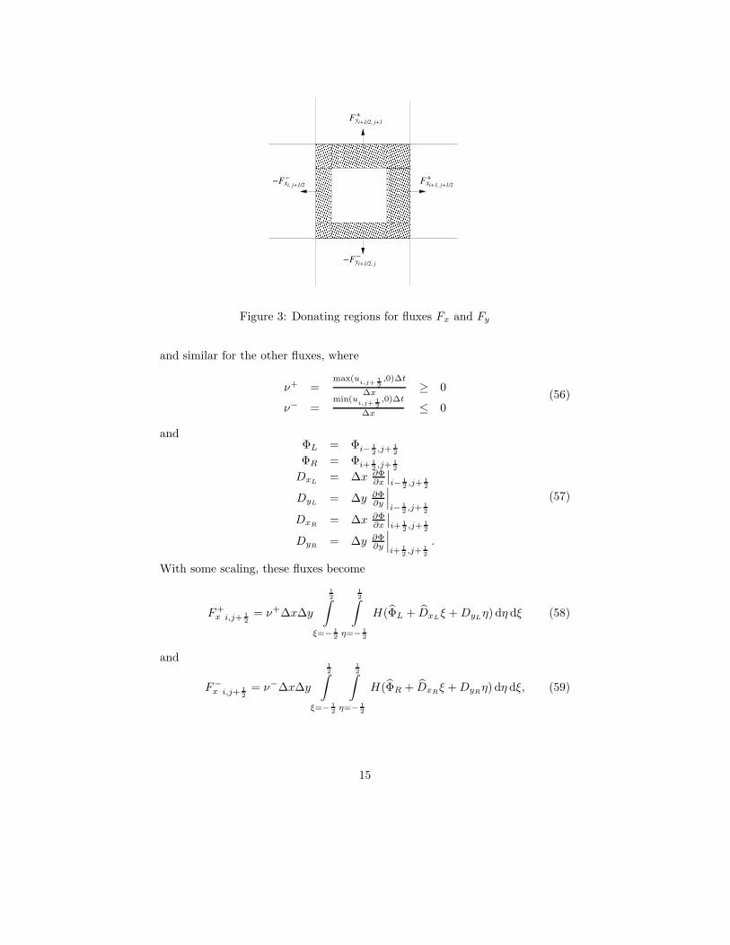
Fxi+1, j+1/2+

Fyi+1/2, j+1+

−Fyi+1/2, j−

−Fxi, j+1/2−

Figure 3: Donating regions for fluxes Fx and Fy

and similar for the other fluxes, where

ν+ =max(u

i,j+ 12

,0)∆t

∆x≥ 0

ν− =min(u

i,j+ 12

,0)∆t

∆x≤ 0

(56)

andΦL = Φi− 1

2,j+ 1

2

ΦR = Φi+ 12,j+ 1

2

DxL= ∆x ∂Φ

∂x

∣∣i− 1

2,j+ 1

2

DyL= ∆y ∂Φ

∂y

∣∣∣i− 1

2,j+ 1

2

DxR= ∆x ∂Φ

∂x

∣∣i+ 1

2,j+ 1

2

DyR= ∆y ∂Φ

∂y

∣∣∣i+ 1

2,j+ 1

2

.

(57)

With some scaling, these fluxes become

F+x i,j+ 1

2= ν+∆x∆y

12∫

ξ=− 12

12∫

η=− 12

H(ΦL + DxLξ + DyL

η) dη dξ (58)

and

F−x i,j+ 1

2= ν−∆x∆y

12∫

ξ=− 12

12∫

η=− 12

H(ΦR + DxRξ + DyR

η) dη dξ, (59)

15

whereΦL = ΦL + 1

2 (1 − ν+)DxL

ΦR = ΦR − 12 (1 + ν−)DxR

DxL= ν+DxL

DxR= −ν−DxR

.

(60)

The integrals of Eqns. (58) and (59) are just Eqn. (45) with Φk replaced by ΦL

and ΦR and Dx replaced by DxLand DxR

respectively. Therefore, Eqns. (47),(48) and (49) are used to evaluate F +

x i,j+ 12

and F−x i,j+ 1

2:

F+x i,j+ 1

2= ν+∆x∆y Ψ|ΦL,DxL

,DyL

F−x i,j+ 1

2= ν−∆x∆y Ψ|ΦR,DxR

,DyR

.(61)

The fluxes in y-direction are obtained in the same way.In Fig. 3 it is shown that overlapping donating regions can exist in the

corners of the cell. Fluid in those overlapping regions is fluxed more than oncethrough different faces. As reported in for example [1], this can be solved byemploying either a multidimensional scheme or flux-splitting. Here the secondapproach has been chosen, for reasons of simplicity. The order of fluxing is:first in x-direction, then in y-direction. Currently the flux-splitting of [46] isadopted:

Ψ∗i+ 1

2,j+ 1

2

=Ψn

i+ 12

,j+ 12

− 1∆x∆y

(Fx

n

i+1,j+ 12

−Fxn

i,j+ 12

)

1− ∆t∆x

(ui+1,j+ 1

2−u

i,j+ 12)

Ψ∗∗i+ 1

2,j+ 1

2

=Ψ∗

i+ 12

,j+ 12

− 1∆x∆y

(Fy

∗

i+12

,j+1−Fy

∗

i+12

,j

)

1− ∆t∆y

(vi+ 1

2,j+1

−vi+1

2,j

)

Ψn+1i+ 1

2,j+ 1

2

= Ψ∗∗ − ∆t

(Ψ∗

ui+1,j+ 1

2−u

i,j+ 12

∆x+ Ψ∗∗

vi+ 1

2,j+1

−vi+ 1

2,j

∆y

).

(62)

Flux redistributing As reported in [46], undershoots and/or overshoots canstill occur. These errors give rise to total mass errors of order 10−4. This isalso experienced in the current research. Mass errors are completely avoidedby redistributing Ψ. The idea is to flux mass out of cells with Ψ > 1 and fluxmass into cells with Ψ < 0. Since the trouble is in the doubly-fluxed regions,the fluxes are firstly taken from the diagonal (i + 1

2 − sign(u), j + 12 − sign(v))

neighboring cells.Assume that cell k has a value Ψn+1

k < 0. Then define a flux F towardsneighboring cell l, so that Ψk = Ψn+1

k − F = 0:

F = Ψn+1k . (63)

In order not to cause unphysical values of Ψl, limit F by

F = min(max(Ψn+1k ,−Ψn+1

l ), 1 − Ψn+1l ), (64)

16

v

u2

7 5 6

4

831

Figure 4: Order of flux redistributing for u > 0 and v > 0

so that 0 ≤ Ψl = Ψn+1l + F ≤ 1. Then make corrections to Φk and Φl by

Ψk = Ψn+1k − F

Ψl = Ψn+1k + F.

(65)

In case of Ψn+1k > 1, the flux F is

F = min(max(Ψn+1k − 1,−Ψn+1

l ), 1 − Ψn+1l ). (66)

In two dimensions, there exist 8 neighboring cells l which can contributeto cell k. The order in which the neighboring cells l are subsequently chosenis depicted in Fig. 4. Note that the first step (in −(sign(u), sign(v))-direction)takes out most of the unphysical Ψ-values, since this is the direction the doubly-fluxed region was fluxed from. It is therefore important to take that neighborfirst. The order of the other neighbors are arbitrary. The values u and v at Ψlocations are interpolated by averaging.

Step 3: Inverse function Having found a new fractional volume Ψn+1,the initial guess of the Level-Set function Φn+1,∗ (after Level-Set advection) ismodified, such that mass is conserved within each computational cell. In otherwords, find (Φ1, Φ2, . . . ), such that

Ψk(Φ1, Φ2, . . . ) − Ψn+1k = 0 ∀k = 1, 2, . . . . (67)

It will be clear that due to the behavior of Ψ no unique solution Φ exists.However, a (small) correction to Φ∗ is searched, where Φ∗ comes from Level-Set advection. A solution Φ is found by the repeating (i.e. iteratively) untilconvergence: leave Φ unmodified in a grid point when the Volume-of-Fluidconstraint is satisfied and make corrections locally when this constraint is notsatisfied. This is achieved by using the inverse function of Ψk as given in Eqn.(47) with respect to argument Φk and employing Picard-iterations. Startingwith (Φn+1,∗

1 , Φn+1,∗2 , . . . ), if at time step n + 1 (Ψ1, Ψ2, . . . ) has to be equal to

17

(Ψn+11 , Ψn+1

2 , . . . ), then the mth iteration is:

Dx = ∆x ∂Φ∂x

∣∣n+1,m

k

Dy = ∆y ∂Φ∂y

∣∣∣n+1,m

k

Φmax = 12 (|Dx| + |Dy|)

Φmid = 12

∣∣∣ |Dy| − |Dx|∣∣∣

(68)

and if Ψn+1,mk 6= Ψn+1

k (else Φn+1,m+1k = Φn+1,m

k )

Φn+1,m+1k =

−Φmax Ψn+1k ≤0

B 0< Ψn+1k <1 − Ψmid

C 1 − Ψmid ≤ Ψn+1k ≤Ψmid

D Ψmid < Ψn+1k <1

Φmax Ψn+1k ≥1,

(69)

where

B =√

2Ψn+1k (Φ2

max − Φ2mid) − Φmax

C = (Ψn+1k − 1

2 )(Φmax + Φmid)

D = −√

2(1− Ψn+1k )(Φ2

max − Φ2mid) + Φmax

(70)

and

Ψmid =1

2

Φmax + 3Φmid

Φmax + Φmid

. (71)

These iterations are repeated until

maxk

|Ψn+1,m+1k − Ψn+1

k | ≤ ε, (72)

where ε is a tolerance, typically

ε = 1 × 10−8. (73)

A graphical overview of the method is depicted in Fig. 5.

3.3 Time-step restrictions

Following [39, 47, 50], an adaptive time stepping procedure is chosen by consid-ering the time-step restrictions due to convection, diffusion and surface tensioneffects. Since the Level-Set function Φ and the Volume-of-Fluid function Ψ areadvected explicitly, the restriction due to advection is:

∆tc =1

|u|max

∆x+ |v|max

∆y

. (74)

The restriction due to surface tension in [47, 50] is

∆ts =1√

σ|κ|max

min(ρ0,ρ1) min(∆x,∆y)2

. (75)

18

Φ n+1

Ψ n

Ψ n+1Φ n+1,*

Φn

−1 f Φ = (Ψ)

−1 f Φ = (Ψ)

flux redistribution

flux y−direction

flux x−direction

n+1,x

level−Set advection

re−initialization

Ψ = (Φ)

Ψ

Φ n+1,x

f

VOF advection

Figure 5: MCLS method: interface advection; Φ: Level-Set function;Ψ: Volume-of-Fluid function

Since the surface tension forces are regularized i.e. σκ is replaced by σκδ(Φ)hand h = min(∆x, ∆y), the restriction becomes

∆ts =1√

|σκδ(Φ)|max

min(ρ0,ρ1)min(∆x,∆y)

. (76)

Diffusion is accounted for implicitly, hence no time-step restriction is encoun-tered. For the time step ∆t finally holds (see e.g. [39])

∆t ≤ CFLmin(∆tc, ∆ts), (77)

where, again following [39, 47, 50], CFL = 12 is used.

4 Applications

The method is applied to show the behavior of the MCLS approach. First ofall, the advection algorithm is tested by advecting an interface by a prescribedvelocity field. Subsequently, the method is illustrated by considering a fallingdrop and a rising bubble respectively.

4.1 Advection tests

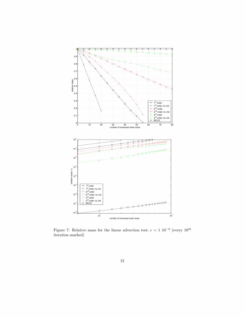
4.1.1 Linear advection

The first advection test is presented in Fig. 6. The velocity field is prescribed

19

R0

2R0

Lx

Ly u

Figure 6: Linear advection test

byu = 0v = −1.

(78)

The dimensions of the computational domain are

Lx = 10Ly = 100,

(79)

which is discretized by a 10x100-mesh. Initially a circle of radius R0 is placedat x = Lx/2 and y = Ly − 2R0. For the case of R0 = 4 (a circle with adiameter of 8 mesh sizes), the relative mass is plotted in Fig. 7 as function ofthe traversed distance of the circle. First-order, second-order and third-ordersimulations are included. Also re-initialization and VOF advection are included.The truncation error of re-initialization is the same the order as the truncationerror of advection. The tolerance in the VOF advection is taken to be:

ε = 1 10−8. (80)

Globally speaking:

• mass is always lost without the VOF advection;

• mass losses are smaller for higher accuracy;

• re-initialization causes much higher mass losses;

• the MCLS method conserves mass up to a specified tolerance.

4.1.2 Zalesak’s rotating disc

The advection test of Zalesak ([25]) is used often in literature to demonstratethe interface-advection algorithm (see e.g. [26, 31, 33, 56] for VOF methods and[39, 40, 45, 46] for Level-Set methods). A slotted disc (Fig. 8) is rotated through

20

0 10 20 30 40 50 60 70 800

0.1

0.2

0.3

0.4

0.5

0.6

0.7

0.8

0.9

1

number of traversed mesh sizes

rela

tive

mas

s

1st order1st order; re−init.2nd order2nd order; re−init.3rd order3rd order; re−init.MCLS

101 10210−8

10−7

10−6

10−5

10−4

10−3

10−2

10−1

100

number of traversed mesh sizes

|rela

tive

mas

s−1|

1st order1st order; re−init.2nd order2nd order; re−init.3rd order3rd order; re−init.MCLS

Figure 7: Relative mass for the linear advection test; ε = 1 10−8 (every 10th

iteration marked)

21

R0

W

W

Figure 8: Zalesak’s slotted disc advection test (on scale)

one revolution around the center of the computational domain. The velocity-field is prescribed by

u = −(y − 12Ly)

v = x − 12Lx.

(81)

The center of the slotted disc (x0, y0)t is located at

x0 = 12Lx

y0 = 34Ly.

(82)

The sizes areLx = Ly

R0 = 320Lx

W = 13R0.

(83)

In Figs. 9 and 10 results are shown for 50×50, 100×100, 150×150 and 200×200mesh sizes. As might be expected from the linear advection discussed in theforegoing, mass is still lost in case of the high-order Level-Set method. For theMCLS method, mass is conserved up to the specified tolerance ε although massis redistributed due to numerical diffusion. Results of the MCLS method arecomparable with VOF/PLIC methods (see aforementioned references). Notethat the Level-Set advection is first-order in case of the MCLS method.

If S represents the interface after one revolution, the length l(S) of S is then

l(S) =

∫

S

dS, (84)

22

0.3 0.4 0.5 0.6 0.7

0.6

0.7

0.8

0.9

50x50

0.3 0.4 0.5 0.6 0.7

0.6

0.7

0.8

0.9

100x100

0.3 0.4 0.5 0.6 0.7

0.6

0.7

0.8

0.9

150x150

0.3 0.4 0.5 0.6 0.7

0.6

0.7

0.8

0.9

200x200

Figure 9: Results for Zalesak’s advection test; shaded: initial contour; dashedlines: 3rd order; solid lines: MCLS

10−1 10010−10

10−9

10−8

10−7

10−6

10−5

10−4

10−3

10−2

10−1

number of revolutions

|rela

tive

mas

s−1|

3rd order; 50x503rd order; 200x200MCLS; 50x50MCLS; 200x200

Figure 10: Relative masses for Zalesak’s advection test; ε = 1 × 10−8 (every50th iteration marked)

23

l(S)l(S0) 50× 50 100× 100 150× 150 200× 200

initial 0.86094 0.98187 0.98804 0.991023rd order 0.49236 0.80940 0.91253 0.93318

MCLS 0.84106 0.95977 0.97020 0.97570

Table 1: Computed interface lengths after one revolution

which can be expressed as (see e.g. [38])

l(S) =

∫

Ω

δ(Φ)|∇Φ| dΩ. (85)

This is approximated by using central differences and regularization of the Diracdelta function (see Eqn. (12)):

l(S) =

∫

Ω

δα(Φ)|∇Φ| dΩ, (86)

where

δα(x) =

0, |x| > α1+cos( πx

α)

2α, |x| ≤ α.

(87)

Note that due to Eqn. (12), the exact value of Φ has no meaning in the Level-Set formulation; only the sign is relevant. The α in Eqn. (86) equals thereforethe α of Eqn. (12). The exact length of the interface is

l(S0) =

(4 + 2π − 2 arctan(

1

2

W

R0) −

W

R0

)R0. (88)

In Table (1) the computed interface lengths are compared with the exact length.‘Initial’ means at t = 0, when errors are made due to the regularization of thedelta function. Furthermore, ‘3rd order’ and ‘MCLS’ correspond to the interfacelengths after one revolution.

Since Φ0 is a distance function, |Φ − Φ0| is a measure for the shift of theinterface after one revolution. A norm of the error e can now be defined as

||e||p =

(∫S|Φ−Φ0

Lx|p dS∫

SdS

) 1p

=

(∫Ω|Φ−Φ0

Lx|p δα(Φ)|∇Φ| dΩ∫

Ωδα(Φ)|∇Φ| dΩ

) 1p

, (89)

where Lx is used to non-dimensionalize Φ and Φ0 is the initial Level-Set function.The results are presented in Fig. 11.

24

10−3 10−2 10−110−4

10−3

10−2

10−1

∆x / L||

e || 1

10−3 10−2 10−110−4

10−3

10−2

10−1

∆x / L

|| e

|| 2

10−3 10−2 10−110−2

10−1

100

∆x / L

| l(S

)/l(S

0 )−1

|

3rd orderMCLS

Figure 11: Errors for Zalesak’s advection test

4.2 Air/water flow

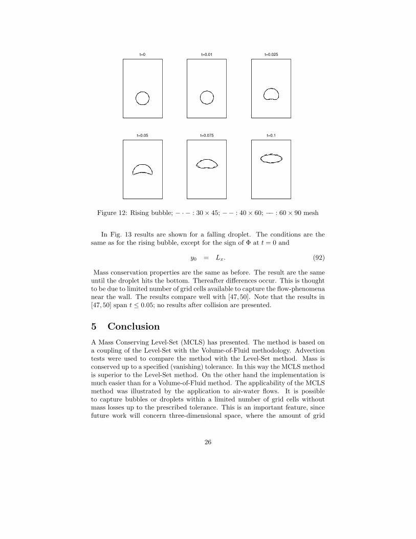
In [47, 50] a two-dimensional rising air bubble in water is considered. The di-mensions and sizes are

Lx = 0.02 mLy = 1 1

2Lx

R0 = 16Lx

x0 = 12Lx

y0 = 12Lx.

(90)

The gravity and material constants are

g = 9.8 ms2 σ = 0.0728 kg

s2

ρw = 103 kgm3 ρa = 1.226 kg

m3

µw = 1.137 10−3 kgms

µa = 1.78 10−5 kgms

,

(91)

where subscripts w and a indicate water and air respectively. Results are shownin Fig. 12 for three different mesh sizes. These are 30× 45, 40× 60 and 60× 90.We take ε = 1 × 10−8. Relative mass losses are of the same order and inagreement with the advection tests. Note that mesh sizes are much smaller thanin [47, 50]. The results are the same for t ≤ 0.025 for all mesh sizes. Thereaftersmall differences occur. The results compare well with [47, 50]. The MCLSmethod seems to result in a more coherent structure at the highly curved partof the interface at t = 0.05. This is thought to be caused by the low resolutionof the grids used here.

25

t=0 t=0.01 t=0.025

t=0.05 t=0.075 t=0.1

Figure 12: Rising bubble; − · − : 30× 45; −− : 40 × 60; −− : 60 × 90 mesh

In Fig. 13 results are shown for a falling droplet. The conditions are thesame as for the rising bubble, except for the sign of Φ at t = 0 and

y0 = Lx. (92)

Mass conservation properties are the same as before. The result are the sameuntil the droplet hits the bottom. Thereafter differences occur. This is thoughtto be due to limited number of grid cells available to capture the flow-phenomenanear the wall. The results compare well with [47, 50]. Note that the results in[47, 50] span t ≤ 0.05; no results after collision are presented.

5 Conclusion

A Mass Conserving Level-Set (MCLS) has presented. The method is based ona coupling of the Level-Set with the Volume-of-Fluid methodology. Advectiontests were used to compare the method with the Level-Set method. Mass isconserved up to a specified (vanishing) tolerance. In this way the MCLS methodis superior to the Level-Set method. On the other hand the implementation ismuch easier than for a Volume-of-Fluid method. The applicability of the MCLSmethod was illustrated by the application to air-water flows. It is possibleto capture bubbles or droplets within a limited number of grid cells withoutmass losses up to the prescribed tolerance. This is an important feature, sincefuture work will concern three-dimensional space, where the amount of grid

26

t=0 t=0.02 t=0.04

t=0.05 t=0.06 t=0.065

Figure 13: Falling droplet; − · − : 30× 45; −− : 40 × 60; −− : 60 × 90 mesh

cells available to an individual entity will decrease considerably. Computing ona larger scale is intended in the near future.

References

[1] S.P. van der Pijl. Free-boundary methods for multi-phase flows. AMA re-port 02-13, Delft University of Technology, 2002. http://ta.twi.tudelft.nl.

[2] S.O.Unverdi and G. Tryggvason. A front-tracking method for viscous, in-compressible, multi-fluid flows. Journal of Computational Physics, 100:25–37, 1992.

[3] A. Esmaeeli and G. Tryggvason. Direct numerical simulations of bubblyflows, part 1, low reynolds number arrays. Journal of FLuid Mechanics,377:313–345, 1998.

[4] G. Agresar, J.J. Linderman, G. Tryggvason, and K.G. Powell. An adaptive,Cartesian, front-tracking method for the motion, deformation and adhesionof circulation cells. Journal of Computational Physics, 143:346–380, 1998.

[5] B. Bunner and G. Tryggvason. Direct numerical simulations of three-dimensional bubbly flows. Physics of Fluids, 11:1967–1969, 1999.

[6] G. Tryggvason, B. Bunner, A. Esmaeeli, D. Juric, N. Al-Rawahi,W. Tauber, J. Han, S. Nas, and Y.-J. Jan. A front-tracking method for

27

the computation of multiphase flow. Journal of Computational Physics,169:708–759, 2001.

[7] C.S. Peskin and B.F. Printz. Improved volume conservation in the compu-tation of flows with immersed elastic boundaries. Journal of ComputationalPhysics, 105:33–46, 1993.

[8] A.M. Roma, C.S. Peskin, and M.J. Berger. An adaptive version of theimmersed boundary method. Journal of Computational Physics, 153:509–534, 1999.

[9] M.-C. Lai and C.S. Peskin. An immersed boundary method with formalsecond-order accuracy and reduced numerical viscosity. Journal of Com-putational Physics, 160:705–719, 2000.

[10] E. Jung and C.S. Peskin. Two-dimensional simulations of valveless pumpingusing the immersed boundary method. SIAM Journal on Applied Mathe-matics, 23(1):19–45, 2001.

[11] J.U. Brackbill, D.B. Kothe, and C. Zemach. A continuum method formodeling surface tension. Journal of Computational Physics, 100:335–354,1992.

[12] W.Shyy, H.S.Udaykumar, M.M. Rao, and R.W. Smith. ComputationalFluid Dynamics with Moving Boundaries. Series in computational andphysical processes in mechanics and thermal sciences. Taylor and Francis,Washington DC, 1996.

[13] H.S. Udaykumar, H.-C. Kan, and W. Shyy R. Tran-Son-Tay. Multiphasedynamics in arbitrary geometries on fixed cartesian grids. Journal of Com-putational Physics, 137:366–405, 1997.

[14] T. Ye, R. Mittal, H.S. Udaykumar, and W. Shyy. An accurate carte-sian grid method for viscous incompressible flows with complex immersedboundaries. Journal of Computational Physics, 156:209–240, 1999.

[15] G. Yang, D.M. Causon, and D.M. Ingram. Calculation of compressibleflows about complex moving geometries using a three-dimensional Carte-sian cut cell method. International Journal for Numerical Methods in Flu-ids, 33:1121–1151, 2000.

[16] H.S. Udaykumar, R. Mittal, P. Rampunggoon, and A. Khanna. A sharpinterface cartesian grid method for simulating flows with complex movingboundaries. Journal of Computational Physics, 174:345–380, 2001.

[17] H.S. Udaykumar, R. Mittal, and P. Rampunggoon. Interface tracking fi-nite volume method for complex solid-fluid interactions on fixed meshes.Communications in Numerical Methods in Engineering, 18:89–97, 2002.

28

[18] T. Ye, W. Shyy, , and J.N. Chung. A fixed-grid, sharp-interface methodfor bubble dynamics and phase change. Journal of Computational Physics,174:781–815, 2001.

[19] F.H. Harlow and J.E. Welch. Numerical calculation of time-dependentviscous incompressible flow of fluid with free surfaces. Physics of Fluids,8:2182–2189, 1965.

[20] S. Chen, B. Johnson, P.E. Raad, and D. Fadda. The surface marker andmicro cell method. International Journal for Numerical Methods in Fluids,25:749–778, 1997.

[21] W.F. Noh and P. Woodward. SLIC (Simple Line Interface Calculations). InA.I. van de Vooren and P.J. Zandbergen, editors, Lecture Notes in Physics,Vol. 59, pages 330–340, New York, 1976. Proceedings of the Fifth Interna-tional Conference on Numerical Methods in Fluid Dynamics, Springer.

[22] T. Yabe, F. Xiao, and T. Utsumi. The constrained interpolation pro-file method for multiphase analysis. Journal of Computational Physics,169:556–593, 2001.

[23] T. Nakamura, R. Tanaka, T. Yabe, and K. Takizawa. A numerical methodfor two-phase flow consisting of seperate compressible and incompressibleregions. Journal of Computational Physics, 174:171–207, 2001.

[24] T. Yabe and F. Xiao. Description of complex and sharp interface with fixedgrids in incopmressible and compressible fluid. Computers and Mathematicswith Applications, 29:1:15–25, 1995.

[25] S.T. Zalesak. Fully multidimensional flux-corrected transport algorithm forfluids. Journal of Computational Physics, 31:335–362, 1979.

[26] M. Rudman. Volume-tracking methods for interfacial flow calculations.International Journal for Numerical Methods in Fluids, 24:671–691, 1997.

[27] C.W. Hirt and B.D. Nichols. Volume of fluid (vof) method for the dynamicsof free boundaries. Journal of Computational Physics, 39:201–225, 1981.

[28] B. Lafaurie, C. Nardone, R. Scardovelli, S. Zaleski, and G. Zanetti. Mod-elling merging and fragmentation in multiphase flows with SURFER. Jour-nal of Computational Physics, 113:134–147, 1994.

[29] M. Rudman. A volume-tracking methods for incompressible multifluid flowwith large density variations. International Journal for Numerical Methodsin Fluids, 28:357–378, 1998.

[30] D. Geuyffier, J. Li, A. Nadim, R. Scardovelli, and S. Zaleski. Volume-of-fluid interface tracking with smoothed surface stress methods for three-dimensional flows. Journal of Computational Physics, 152:423–456, 1999.

29

[31] W.J. Rider and D.B. Kothe. Reconstructing volume tracking. Journal ofComputational Physics, 141:112–152, 1998.

[32] M. Renardy, Y. Renardy, and J. Li. Numerical simulation of moving contactline problems using a volume-of-fluid method. Journal of ComputationalPhysics, 171:243–263, 2001.

[33] D.J.E. Harvie and D.F. Fletcher. A new volume of fluid advection al-gorithm: the defined donating region scheme. International Journal forNumerical Methods in Fluids, 35:151–172, 2001.

[34] W. Mulder, S. Osher, and J.A. Sethian. Computing interface motion incompressible gas dynamics. Journal of Computational Physics, 100:209–228, 1992.

[35] J.A. Sethian. Level Set Methods and Fast Marching Methods. Cambridgemonographs on applied and computational mathematics. Cambridge Uni-versity Press, Cambridge, 1999.

[36] J.A. Sethian. Evolution, implementation, and application of level set andfast marching methods for advancing fronts. Journal of ComputationalPhysics, 169:503–555, 2001.

[37] S. Osher and R.P. Fedkiw. Level set methods: An overview and some recentresults. Journal of Computational Physics, 169:463–502, 2001.

[38] Y.C. Chang, T.Y. Hou, B. Merriman, and S. Osher. A level set formula-tion of eulerian interface capturing methods for incompressible fluid flows.Journal of Computational Physics, 124:449–464, 1996.

[39] M. Sussman, E. Fatemi, P. Smereka, and S. Osher. An improved level setmethod for incompressible two-phase flows. Computers and Fluids, 27:663–680, 1998.

[40] M. Sussman and E. Fatemi. An efficient, interface-preserving level setredistancing algorithm and its application to interfacial incompressible fluidflow. SIAM Journal on Scientific Computing, 20(4):1165–1191, 1999.

[41] H. Haj-Hariri and Q. Shi. Thermocapillary motion of deformable dropsat finite Reynolds and Marangoni numbers. Physics of Fluids, 9:845–855,1997.

[42] M. Sussman, A.S. Almgren, J.B. Bell, P. Colella, L.H. Howell, and M.L.Welcome. An adaptive level set approach for incompressible two-phaseflows. Journal of Computational Physics, 148:81–124, 1999.

[43] L.L. Zheng and H. Zhang. An adaptive level set method for moving-boundary problems: Application to droplet spreading and solidification.Numerical Heat Transfer, Part B, 37:437–454, 2000.

30

[44] M. Sussman, P. Smereka, and S. Osher. A level set approach for comput-ing solutions to incompressible two-phase flow. Journal of ComputationalPhysics, 114:146–159, 1994.

[45] D. Enright, R. Fedkiw, J. Ferziger, and I. Mitchell. A hybrid particle levelset method for improved interface capturing. UCLA CAM Report 02-04,University of California, Los Angeles, 2002.

[46] M. Sussman and E.G. Puckett. A coupled level set and volume-of-fluidmethod for computing 3D and axisymmetric incompressible two-phaseflows. Journal of Computational Physics, 162:301–337, 2000.

[47] M. Kang, R.P. Fedkiw, and D.Q. Nguyen. A boundary condition capturingmethod for multiphase incompressible flow. UCLA CAM Report 99-27,University of California, Los Angeles, 1999.

[48] Z. Li and M.-C. Lai. The immersed interface method for the navier-stokesequations with singular forces. Journal of Computational Physics, 171:822–842, 2001.

[49] J.J.I.M. van Kan. A second-order accurate pressure correction method forviscous incompressible flow. SIAM J. Sci. Stat. Comp., 7:870–891, 1986.

[50] M. Kang, R.P. Fedkiw, and X.-D. Liu. A boundary condition capturingmethod for multiphase incompressible flow. Journal of Scientific Comput-ing, pages 323–360, 2000.

[51] X.-D. Liu, R.P. Fedkiw, and M. Kang. A boundary condition capturingmethod for Poisson’s equation on irregular domains. Journal of Computa-tional Physics, 160:151–178, 2000.

[52] R.J. Leveque and Z. Li. Immersed interface methods for Stokes flow withelastic boundaries or surface tension. SIAM Journal on Scientific Comput-ing, 18(3):709–735, 1997.

[53] A. Wiegmann and K.P. Bube. The explixit-jump immersed interfacemethod: finite difference methods for PDEs with piecewise smooth so-lutions. SIAM Journal on Numerical Analysis, 37(3):827–862, 2000.

[54] T.Y. Hou, Z. Li, S. Osher, and H. Zhao. A hybrid method for moving in-terface problems with application to the Hele-Shaw flow. Journal of Com-putational Physics, 134:236–252, 1997.

[55] Z. Li and S.R. Lubkin. Numerical analysis of interfacial two-dimensionalStokes flow with discontinuous viscosity and variable surface tension. In-ternational Journal for Numerical Methods in Fluids, 37:525–540, 2001.

[56] D.J.E. Harvie and D.F. Fletcher. A new volume of fluid advection algo-rithm: the stream scheme. Journal of Computational Physics, 162:1–32,2000.

31