Embed Size (px)
Citation preview
Delaunay Surfaces
Enrique Bendito∗, Mark J. Bowick** and Agustın Medina**Departament Matematica Aplicada IIIUniversitat Politecnica de Catalunya,
Barcelona, Spain.**Physics DepartmentSyracuse University
Syracuse, NY 13244-1130, USA
Abstract
We derive parametrizations of the Delaunay constant mean curvature surfaces ofrevolution that follow directly from parametrizations of the conics that generate thesesurfaces via the corresponding roulette. This uniform treatment exploits the naturalgeometry of the conic (parabolic, elliptic or hyperbolic) and leads to simple expressionsfor the mean and Gaussian curvatures of the surfaces as well as the construction ofnew surfaces.
1 Preliminaries
The surfaces of revolution with constant mean curvature (CMC) were introduced and com-pletely characterized by C. Delaunay more than a century ago [2]. Delaunay’s formulationof the problem leads to a non–linear ordinary differential equation involving the radius ofcurvature of the plane curve that generates the surface, which can be also characterized vari-ationally as the surface of revolution having a minimal lateral area with a fixed volume (see[3]). Delaunay showed that the above differential equation arises geometrically by rolling aconic along a straight line without slippage. The curve described by a focus of the conic,the roulette of the conic, is then the meridian of a surface of revolution with constant meancurvature, where the straight line is the axis of revolution. These CMC surfaces of revolu-tion are called Delaunay surfaces. Apart from the elementary cases of spheres and cylinders,there are three classes of Delaunay surfaces, the catenoids, the unduloids and the nodoids,corresponding to the choice of conic as a parabola, an ellipse or a hyperbola, respectively.
∗e-mail: [email protected]
1
arX
iv:1
305.
5681
v1 [
mat
h.D
G]
24
May
201
3

Traditionally the roulettes have been characterized using polar coordinates centered atthe focus of the conic [1, 6, 5, 3, 8, 9, 4, 7]. The methods emplyed in these papers are basedon solving certain ordinary differential equations that, in one way or another, depend onthe variational characterization of the CMC surfaces. Although Ref. [1] does suggest thepossibility of using the cartesian coordinates of the roulettes with the tangent to the conicas the abscissa, this idea is never developed.
Here we obtain parametrizations of the roulettes, and therefore of the correspondingDelaunay surfaces, directly from the parametrizations of the conics. This leads directlyto concise expressions for all the key differential geometric characteristics of Delaunay sur-faces. In our approach the unduloid is described with trigonometric functions, whereas thecatenoid and the nodoid are described with hyperbolic functions. This yields simple expres-sions for the Gaussian curvature, total curvature and mean curvature as well as the lengthof roulettes. The mean curvature of an unduloid, in particular, is given by the inverse ofthe distance between the vertices of the corresponding ellipse, whereas the mean curvatureof a nodoid is given by minus the inverse of the distance between the vertices of the corre-sponding hyperbola. The parametrizations presented here also give rise to a straightforwardconstruction of nodoids, both when viewed as simple parts (generated by a focus) or whenthey are composed of several individual parts or a periodic repetition of simple parts.
For the sake of completeness, we finish this section by presenting some well-known resultsabout regular surfaces of revolution, as well as a very simple proof of the Gauss-Bonetttheorem for this class of surfaces.
Let f, g : [t1, t2] −→ R be smooth functions with f > 0, and S the surface of revolutionparametrized by xxxxxxxxxxxxxx : [t1, t2]× [v1, v2] −→ R3
xxxxxxxxxxxxxx(t, v) =(f(t) cos(v), f(t) sin(v), g(t)
).
The coefficients of the first and second fundamental forms of S are given by
E = 〈xxxxxxxxxxxxxxt, xxxxxxxxxxxxxxt〉 = (f ′)2 + (g′)2, F = 〈xxxxxxxxxxxxxxt, xxxxxxxxxxxxxxv〉 = 0, G = 〈xxxxxxxxxxxxxxv, xxxxxxxxxxxxxxv〉 = f 2;
L = 〈xxxxxxxxxxxxxxtt, nnnnnnnnnnnnnn〉 =f ′g′′ − f ′′g′(
(f ′)2 + (g′)2)1/2 , M = 〈xxxxxxxxxxxxxxtv, nnnnnnnnnnnnnn〉 = 0, N = 〈xxxxxxxxxxxxxxvv, nnnnnnnnnnnnnn〉 =
fg′((f ′)2 + (g′)2
)1/2 ,where
nnnnnnnnnnnnnn =xxxxxxxxxxxxxxt × xxxxxxxxxxxxxxv|xxxxxxxxxxxxxxt × xxxxxxxxxxxxxxv|
=1(
(f ′)2 + (g′)2)1/2(− g′ cos(v),−g′ sin(v), f ′
),
is the unit normal to S. The Gaussian curvature is given by
K =LN
EG=
g′(f ′g′′ − f ′′g′)
f(
(f ′)2 + (g′)2)2 ,
2

whereas the mean curvature, H, is given by
2H = k1 + k2 =L
E+N
G=
f ′g′′ − f ′′g′((f ′)2 + (g′)2
)3/2 +g′
f(
(f ′)2 + (g′)2)1/2 ,
where k1 and k2 are the two principal curvatures.
Now consider a curve α in S parametrized by the arc length s. For any point p = α(s) wechoose a vector uuuuuuuuuuuuuu(s) in the tangent space at p such that {α′(s), uuuuuuuuuuuuuu(s)} is a positively orientedorthonormal basis of the tangent space at p; that is, α′(s) × uuuuuuuuuuuuuu(s) = nnnnnnnnnnnnnn(α(s)). The geodesiccurvature kg(s) of α at s is then given by
kg(s) = 〈α′′(s), uuuuuuuuuuuuuu(s)〉.
If the curve is chosen to be a meridian of S, α(t) = xxxxxxxxxxxxxx(t, v0), then kg = 0, whereas if it is aparallel, β(v) = xxxxxxxxxxxxxx(t0, v), then its geodesic curvature is given by
kg(t0) =f ′(t0)
f(t0)(
(f ′(t0))2 + (g′(t0))2)1/2 .
Lemma 1.1. If C1 and C2 are the boundary parallels of S with the orientation induced byS then ∫
S
Kdσ +
∫C1
kg(t1)d`+
∫C2
kg(t2)d` = 0.
Proof. Observe first that kg(t)|xxxxxxxxxxxxxxv| =f ′(t)(
(f ′(t))2 + (g′(t))2)1/2 and hence
(kg|xxxxxxxxxxxxxxv|
)′=
g′(f ′′g′ − f ′g′′
)(
(f ′)2 + (g′)2)3/2 = −K|xxxxxxxxxxxxxxt| |xxxxxxxxxxxxxxv|.
On the other hand,∫S
Kdσ =
∫ v2
v1
∫ t2
t1
K|xxxxxxxxxxxxxxt| |xxxxxxxxxxxxxxv|dtdv = −∫ v2
v1
∫ t2
t1
(kg|xxxxxxxxxxxxxxv|
)′dtdv
=
∫ v2
v1
kg(t1)|xxxxxxxxxxxxxxv(t1, v)|dv −∫ v2
v1
kg(t2)|xxxxxxxxxxxxxxv(t2, v)|dv = −∫C1
kg(t1)d`−∫C2
kg(t2)d`.
If v2 − v1 = 2π, then S is homeomorphic to an annulus with null Euler characteristic.Otherwise, it is a simple region whose Euler characteristic equals 1 and the sum of the anglesat the four boundary vertices, formed by the tangents to the boundary curves oriented withthe orientation induced by S, equals 2π.
3

2 The Roulettes of the conics
When a curve rolls, without slipping, on a fixed curve, each point of the rolling curve tracesanother curve known as a roulette. In Figure 1 (left), we show the trace generated by thepoint F = (F1, F2), associated with a given curve C, when it rolls on a straight line. Theabscissa F1 of the roulette coincides with Q1, i.e., the length of the arc of the curve from Poto P , minus the value P1 − Q1. We can interchange the roles of the conic and its tangentby considering a fixed conic and a moving tangent. The locus of the points Q thus obtainedis called the pedal curve of C with respect to F . Here we are interested in the roulettesgenerated by the conic foci when they roll over a tangent line.
The parametric description of the parabola, the ellipse and the hyperbola are given re-spectively by
α(t) =(b sinh2(t), 2b sinh(t)
),
β(t) =(a cos(t), b sin(t)
),
γ(t) =(a cosh(t), b sinh(t)
),
where a, b > 0 and t ∈ [t1, t2] ⊂ R.
In Figure 1 (right), we show a parabola, with the perpendicular from F onto the tangentof the parabola at P . This situation is equivalent to the general case and we apply the samecriteria to give a parameterization of this roulette.
Figure 1: Roulette (left) and Parabola (right).
The arc length for the parabola from t0 is
s =
∫ t
t0
|α′(u)|du = b(t+ sinh(t) cosh(t)).
4

The length of the segment PQ is b sinh(t) cosh(t) yielding an abscissa
gc(t) = s− b sinh(t) cosh(t) = bt.
Computing fc(t), the length of the segment FQ, shows that the roulette associated with thefocus of the parabola is the catenary
A(t) = (gc(t), fc(t)) = (bt, b cosh (t)) .
Note also that|A′(t)| = b cosh(t),
and the arc length is given by
`c(t) =
∫ t
t0
|A′(z)| dz = b sinh(z)∣∣∣tt0.
Figure 2: Ellipse (left) and Hyperbola (right).
For the ellipse, Figure 2 (left), take b < a and c =√a2 − b2. The arc length from t0 to t
is
s =
∫ t
t0
|β′(z)|dz =
∫ t
t0
√a2 − c2 cos2(z) dz.
In this case two curves are generated. The first one corresponds to choosing the focus Fclosest to the tangent. By computing the length of the segment PQ and substracting it fromthe above arc, we find that the abscissa is
g1u(t) =
∫ t
t0
√a2 − c2 cos2(z)dz − c sin(t) (a− c cos(t))√
a2 − c2 cos2(t).
5

In addition, the ordinate is given by the length of the segment FQ; namely
f 1u(t) =
b (a− c cos(t))√a2 − c2 cos2(t)
.
B1(t) = (g1u(t), f1u(t)) is therefore the parametrization of the roulette generated by the focus
of the ellipse. One finds
|B′1(t)| =ab
a+ c cos(t),
and the arc length is given by
`1u(t) =
∫ t
t0
|B′1(z)|dz = 2a arctan
(√a− ca+ c
tan(z
2
))∣∣∣∣∣t
t0
.
In the same way, if we chooose the other focus F ′, it follows after computing the lengthof PQ′ that the abscissa is
g2u(t) =
∫ t
t0
√a2 − c2 cos2(z)dz − c sin(t) (a+ c cos(t))√
a2 − c2 cos2(t),
and the ordinate is the length of the segment F ′Q′; namely
f 2u(t) =
b (a+ c cos(t))√a2 − c2 cos2(t)
.
B2(t) = (g2u(t), f2u(t)) is therefore the parametrization of the roulette generated by the focus
F ′. One now finds
|B′2(t)| =ab
a− c cos(t),
and an arc length
`2u(t) =
∫ t
t0
|B′2(z)|dz = 2a arctan
(√a+ c
a− ctan(z
2
))∣∣∣∣tt0
.
Observe in particular that arctan(√
a+ca−c
)+ arctan
(√a−ca+c
)= π
2and then the sum of the
length of the two curves for t ∈ (−π2, π2) is 2πa.
The roulette of the focus of an ellipse is called an undulary. It is clear that we do notneed to consider both foci for an ellipse. Specifically, if we consider the ellipse described bytaking t ∈ [−π, π], the curve generated by the focus F is the same as the curve that resultsfrom joining the two curves generated by both foci F and F ′ with t ∈ [−π/2, π/2] only. Weconsider both foci to make manifest the constructive paralelism between these roulettes andthe roulettes of the hyperbola.
6

Consider now the case of the hyperbola, as shown Figure 2 (right). Taking c =√a2 + b2,
the arc length from t0 to t is
s =
∫ t
t0
|γ′(z)|dz =
∫ t
t0
√c2 cosh2(z)− a2 dz.
For the first roulette we consider the focus F closest to the tangent. By computing thelength of the segment PQ it then follows that the abscissa is
g1n(t) =
∫ t
t0
√c2 cosh2(z)− a2 dz − c sinh(t) (c cosh(t)− a)√
c2 cosh2(t)− a2,
whereas its ordinate is given by the length of FQ, namely,
f 1n(t) =
b (c cosh(t)− a)√c2 cosh2(t)− a2
.
C1(t) = (g1n(t), f 1n(t)) is therefore the parametrization of the roulette generated by the focus
F . One finds
|C ′1(t)| =ab
c cosh(t) + a,
with arc length given by
`1(t) =
∫ t
t0
|C ′1(z)|dz = 2a arctan
(√c− ac+ a
tanh(z
2
))]tt0
.
In particular, the length of C1 with t ∈ (−∞,∞) is 4a arctan(√
c−ac+a
).
Figure 3: Roulettes B1 and B2 (left) and roulettes C1 and C2 (right).
Taking the focus F ′ instead one finds, after computing the length of PQ′, that the abscissais
g2n(t) =
∫ t
t0
√c2 cosh2(z)− a2 dz − c sinh(t) (c cosh(t) + a)√
c2 cosh2(t)− a2,
7

and the ordinate is the length of the segment F ′Q′, namely,
f 2n(t) =
b (c cosh(t) + a)√c2 cosh2(t)− a2
.
C2(t) = (g2n(t), f 2n(t)) is therefore the parametrization of the roulette generated by the focus
F ′. Now
|C ′2(t)| =ab
c cosh(t)− a,
and the arc length is given by
`2(t) =
∫ t
t0
|C ′2(z)|dz = 2a arctan
(√c+ a
c− atanh
(z2
))]tt0
.
The sum of the length of the two branches of the curves for t ∈ (−∞,∞) is again 2πa. Theroulette of the focus of a hyperbola is called a nodary.
In Figure 3 we display the roulettes generated by the foci of the ellipse (left) and thehyperbola (right). B1 and C1 are the curves with increasing slope, while B2 and C2 are thecurves with decreasing slope.
Figure 4: Pedal curves of the ellipse and the hyperbola. Left: arc of the circle (black),whose length coincides with the length of the curve B1 and arc of the circle (green), whoselength coincides with the length of the curve B2. Right: arc of the circle (black), whoselength coincides with the length of the curve C1 and arc of the circle (green) whose lengthcoincides with the length of the curve C2.
In Figure 4 we display the pedal curves of the ellipse (left) and of the hyperbola (right).Both are circles of diameter equal to the distance between the vertices of the conic. It isknown that when a curve rolls on a straight line the arc of the roulette is equal to thecorresponding arc of the pedal. Here we can see this directly. If we consider, for instance,
the curve C1 and denote x = arctan(√
c−ac+a
), then
sin(2x) =b
ccos(2x) =
a
c,
8

and so
4a arctan
(√c− ac+ a
)= 2a arctan
(b
a
).
That is, the length of the curve C1 coincides with the length of the associated pedal curve –see Figure 4 (right in black).
Figure 5: Family of roulettes B1 ∪B2 and C1 ∪ C2 of length 2πa.
In Figure 5 we display a family of roulettes with length 2πa. Each of these rouletes wasgenerated by a conic with major axis a. The straight segment corresponds to a curve oftype B in the limiting case b = a. This is followed by a set of elliptical roulettes from b = auntil the next limiting case b = 0, corresponding to a semicircumference of radius 2a. Theremaining roulettes correspond to curves of type C, ranging from the limiting case b = 0,again the same semicircumference, until b =∞, which is the circle of radius a shown in thefigure.
Figure 6: Left: Location of the roulettes in Figure 5 with respect to the abscissa axis.Right: a family of roulettes of type B1 (green) and C1 (red) separated by a catenary (blue).
In Figure 6 (left) we show the same family of roulettes shown in Figure 5, but to theheight, with respect to the abscissa axis, at which it has been generated by the focus of the
9

corresponding conic. Observe that the limiting circumference of radius a would have thecenter at height b = ∞. In Figure 6(right) we display the asymptotic role of the catenaryseparating two families of curves B1 and C1. In this case the corresponding conics don’thave the parameter a constant, and both families tends to the catenary as the parameter agrows.
3 The Delaunay Surfaces
In this section we study Delaunay surfaces and derive analytical expressions for their mostimportant differential geometric properties. The Delaunay surfaces are surfaces of revolutionand therefore the key to their properties lie in their meridians, which here are the roulettesof the foci of the conics discussed in the previous section. The Delaunay surfaces are thusthe surfaces of revolution generated by the curves A(t), B1(t), B2(t), C1(t) and C2(t). Wenext describe the parametrization, the coefficients of the first and second fundamental formsof each one of these surfaces and their curvatures. The entire differential structure has aramarkably transparent dependence on the parameters that characterize each conic.
Catenoid: xxxxxxxxxxxxxx(t, v) =(fc(t) cos(v), fc(t) sin(v), gc(t)
), – see Figure 7. We have
xxxxxxxxxxxxxxt = (b sinh(t) cos(v), b sinh(t) sin(v), b) ,
xxxxxxxxxxxxxxv = (−b cosh(t) sin(v), b cosh(t) cos(v), 0) .
The unit normal vector at (t, v) is given by
nnnnnnnnnnnnnnc(t, v) =
(− cos(v)
cosh(t),− sin(v)
cosh(t), tanh(t)
).
The non–vanishing coeficients of the first and the second fundamental form, and the principalcurvatures, the mean curvature and the Gaussian curvature are,
E = b2 cosh2(t), G = b2 cosh2(t), L = −b, N = b,
k1 =−1
b cosh2(t), k2 =
1
b cosh2(t), H = 0, K =
−1
b2 cosh4(t).
The geodesic curvature of a parallel is
kg =sinh(t)
b cosh2(t),
and the total curvature of the catenoid is∫xxxxxxxxxxxxxxKdσ = −(v2 − v1) tanh(t)
∣∣∣t2t1.
10

Figure 7: The catenoid.
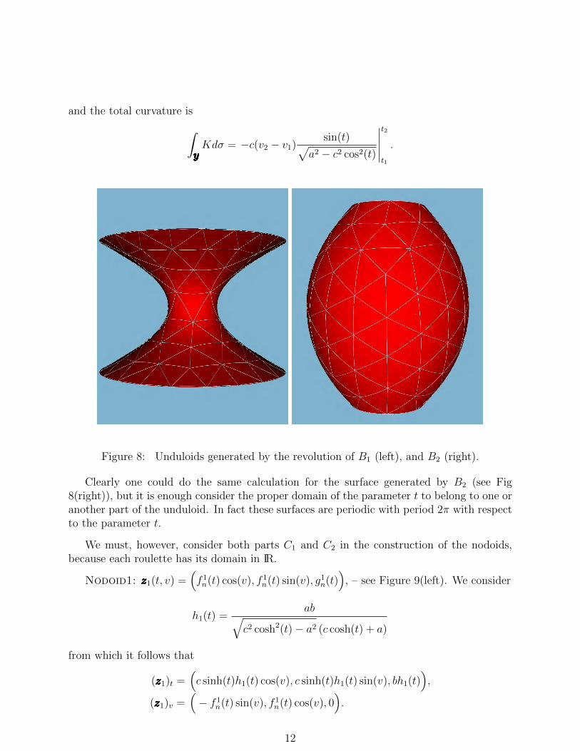
Unduloid: yyyyyyyyyyyyyy(t, v) =(f 1u(t) cos(v), f 1
u(t) sin(v), g1u(t)), – see Figure 8 (left). Considering
hu(t) =ab√
a2 − c2 cos2(t) (a+ c cos(t))
it follows that
yyyyyyyyyyyyyyt = (c sin(t)hu(t) cos(v), c sin(t)hu(t) sin(v), bhu(t)) ,
yyyyyyyyyyyyyyv = (−f 1u(t) sin(v), f 1
u(t) cos(v), 0) .
The unit normal vector at (t, v) is given by
nnnnnnnnnnnnnnu(t, v) =
(−b cos(v)√a2 − c2 cos2(t)
,−b sin(v)√a2 − c2 cos2(t)
,c sin(t)√
a2 − c2 cos2(t)
).
E =a2b2
(a+ c cos(t))2, G =
b2 (a− c cos(t))
(a+ c cos(t)),
L =−ab2c cos(t)
(a2 − c2 cos2(t)) (a+ c cos(t)), N =
b2
a+ c cos(t),
k1 =−c cos(t)
a(a− c cos(t)), k2 =
1
a− c cos(t),
H =1
2a, K =
−c cos(t)
a (a− c cos(t))2.
The geodesic curvature of a parallel is
kg =−c sin(t)
b(a− c cos(t)),
11
and the total curvature is∫yyyyyyyyyyyyyyKdσ = −c(v2 − v1)
sin(t)√a2 − c2 cos2(t)
∣∣∣∣∣t2
t1
.
Figure 8: Unduloids generated by the revolution of B1 (left), and B2 (right).
Clearly one could do the same calculation for the surface generated by B2 (see Fig8(right)), but it is enough consider the proper domain of the parameter t to belong to one oranother part of the unduloid. In fact these surfaces are periodic with period 2π with respectto the parameter t.
We must, however, consider both parts C1 and C2 in the construction of the nodoids,because each roulette has its domain in IR.
Nodoid1: zzzzzzzzzzzzzz1(t, v) =(f 1n(t) cos(v), f 1
n(t) sin(v), g1n(t)), – see Figure 9(left). We consider
h1(t) =ab√
c2 cosh2(t)− a2 (c cosh(t) + a)
from which it follows that
(zzzzzzzzzzzzzz1)t =(c sinh(t)h1(t) cos(v), c sinh(t)h1(t) sin(v), bh1(t)
),
(zzzzzzzzzzzzzz1)v =(− f 1
n(t) sin(v), f 1n(t) cos(v), 0
).
12

The unit normal vector at (t, v) is given by
nnnnnnnnnnnnnn1(t, v) =
−b cos(v)√c2 cosh2(t)− a2
,−b sin(v)√
c2 cosh2(t)− a2,
c sinh(t)√c2 cosh2(t)− a2
.
Figure 9: Nodoids generated by the revolution of C1 (left) and C2 (right).
E =a2b2
(c cosh(t) + a)2, G =
b2 (c cosh(t)− a)
c cosh(t) + a,
L =−ab2c cosh(t)(
c2 cosh2(t)− a2)
(c cosh(t) + a), N =
b2
c cosh(t) + a,
k1 =−c cosh(t)
a(c cosh(t)− a), k2 =
1
c cosh(t)− a,
H =−1
2a, K =
−c cosh(t)
a (c cosh(t)− a)2.
The geodesic curvature of a parallel is
kg =c sinh(t)
b(c cosh(t)− a),
and the total curvature is∫zzzzzzzzzzzzzz1
Kdσ = −c(v2 − v1)sinh(t)√
c2 cosh2(t)− a2
∣∣∣∣∣∣t2
t1
.
Nodoid2: zzzzzzzzzzzzzz2(t, v) =(f2(t) cos(v), f2(t) sin(v), g2(t)
), – see Figure 9(right). We consider
h2(t) =−ab√
c2 cosh2(t)− a2 (c cosh(t)− a)
13

Figure 10: Left: Closed nodoid (compact without boundary), connected sum of 4 tori.Right: Connected compact nodoid with boundary.
from which it follows that
(zzzzzzzzzzzzzz2)t =(c sinh(t)h2(t) cos(v), c sinh(t)h2(t) sin(v), bh2(t)
),
(zzzzzzzzzzzzzz2)v =(− f2(t) sin(v), f2(t) cos(v), 0
).
The unit normal vector at (t, v) is given by
nnnnnnnnnnnnnn2(t, v) =
b cos(v)√c2 cosh2(t)− a2
,b sin(v)√
c2 cosh2(t)− a2,− c sinh(t)√
c2 cosh2(t)− a2
.
E =a2b2
(c cosh(t)− a)2, G =
b2 (c cosh(t) + a)
c cosh(t)− a,
L =−ab2c cosh(t)(
c2 cosh2(t)− a2)
(c cosh(t)− a), N =
−b2
c cosh(t)− a,
k1 =−c cosh(t)
a(c cosh(t) + a), k2 =
−1
c cosh(t) + a,
H =−1
2a, K =
c cosh(t)
a (c cosh(t) + a)2.
The geodesic curvature of a parallel is
kg =−c sinh(t)
b(c cosh(t) + a).
The total curvature is
∫zzzzzzzzzzzzzz2
Kdσ = c(v2 − v1)sinh(t)√
c2 cosh2(t)− a2
∣∣∣∣∣∣t2
t1
.
14

Figure 11: Planar sections containing the revolution axis of a family of Delaunay surfaceswith constant volume. From the outside-in: cylinder (black), unduloids (green), catenoid(red), nodoids (blue), catenoid (red) and unduloids (green).
Fig. 10 illustrates the versatility of the parameterization of nodoids adopted here. Weavoid the periodic extension of nodoids with both positive and negative Gaussian curvature,maintain the orientability. preserve the C∞ class and find new surfaces both closed and withboundary.
Delaunay surfaces are characterized by minimizing the area with fixed boundaries andconstant volume. Here we illustrate the versatility of our formulation by finding a surfacewhich satisfies these conditions. Consider a plane curve (f(t), g(t)). The volume enclosed byits surface of revolution is given by π
∫ t1t0f 2(t)g′(t)dt and the end points by (f(t0), g(t0)) =
(f0, g0) and (f(t1), g(t1)) = (f1, g1).
Consider for example the symmetric nodoid generated by a roulette C1 such that theenclosed volume is 1 and the radius is 1 at the end points ±t0. The equations to solve for aand b are then
πab4∫ t0
−t0
(c cosh(t)− a)
(c cosh(t) + a)2√c2 cosh2(t)− a2
dt = 1,
b (c cosh(t0)− a)√c2 cosh2(t0)− a2
= 1.
In Fig 11 we present planar sections that contain the common axis of revolution of severalDelaunay surfaces with enclosed volume equal to 1 and radius 1 at the boundaries. Notethat the solutions depend on t0.
Finally the paremetrizations developed here have proven extremely useful in analytic
15

and computational explorations of the structure of crystalline particle arrays on Delaunaysurfaces as realized experimentally in capillary bridges [10].
Acknowledgments. This work has been partly supported by the Spanish Research Council(Comision Interministerial de Ciencia y Tecnologıa,) under project MTM2010-19660. Thework of M.J.B. was also supported by the National Science Foundation through Grant No.DMR-1004789 and by funds from the Soft Matter Program of Syracuse University.
References
[1] W.H. Besant, Notes on Roulettes and Glissettes, Deighton, Bell and Co. (1890).
[2] C. Delaunay, Sur la surface de revolution dont la courbure moyenne est constante, J.Math. Pures et Appliques 6 (1841), 309–320.
[3] J. Eells, The surfaces of Delaunay, Math. Intelligencer 9 (1987), 53–57.
[4] M. Hadzhilazova, I.M. Mladenov, J. Oprea, Undoloids and their geometry, in ArchivumMatematicum (Brno) 43 (2007), 417–429.
[5] W.-Y. Hsiang, W.-C. Yu, A Generalization of a Theorem of Delaunay, J. DifferentialGeom. 16 (1981), 161–177.
[6] K. Kenmotsu, Surfaces of revolution with prescribed mean curvature, Tohoku Math. J.32 (1980), 147–153.
[7] M. Koiso and B. Palmer, Rolling construction for anisotropic Delaunay surfaces, PacificJ. of Math. 234 (2008), 345-378.
[8] I.M. Mladenov, Delaunay surfaces revisited, C. R. Bulg. Acad. Sci. 55 (2002), 19–24.
[9] W. Rosseman, The first bifurcation point for Delaunay nodoids, Experimental Mathe-matics 14 (2005), 331–342.
[10] E. Bendito, M.J. Bowick, A. Medina and Z. Yao, Crystalline Particle Packings onConstant Mean Curvature (Delaunay) Surfaces, arXiv:1305.1551 .
16