Embed Size (px)
Citation preview

DELAMINATION MODELLING AND
TOUGHENING MECHANISMS OF A WOVEN
FABRIC COMPOSITE
Tadayoshi Yamanaka
Department of Mechanical Engineering
McGill University, Montreal
February 2011
A thesis submitted to McGill University
in partial fulfillment of the requirements for the degree of
Doctor of Philosophy
© Tadayoshi Yamanaka, 2011

ii
Imagination is more important than knowledge.
Albert Einstein(1879 - 1955)

iii
Abstract
Efficient and accurate numerical simulation methods for the damage tolerance
analysis and fatigue life prediction of fibre reinforced polymers are in high
demand in industry. Problems arise in the development of such a simulation
method due to the limitations from numerical methods, i.e., delamination
modelling, and understanding of damage mechanism of woven fabric
composites.
In order to provide effective and accurate delamination modelling, a new crack
modelling method by using the finite element method is proposed in this study.
The proposed method does not require additional degrees-of-freedom in order
to model newly created crack/delamination surfaces. The accuracy of
delamination growth simulation by the proposed method and that of a
commercial FEA package are in good agreement.
The damage mechanisms of five harness satin weave fabric composite is studied
by creating a multiscale finite element model of a double cantilever beam
specimen. The weft and warp yarns, where the gaps are filled with matrix, are
individually modeled. Cohesive zone model elements are pre-located within the
matrix and interfaces of matrix-yarns and weft-yarns and warp yarns. These
meso-scale parts are bonded with homogeneous parts that are used to model
regions where no damage is expected. This constitutes a multiscale model of a
DCB specimen. The simulation results are in good agreement with the lower
bound of experimental results. The toughening mechanism contributed from the
weave structure was revealed.
This study contributes to knowledge by introducing crack modelling methods
and by providing more information in order to understand damage mechanisms
of 5HS weave fabric composite laminates during delamination growth.

iv
Résumé
Les méthodes de simulation numériques efficaces et exactes pour l'analyse de
l’endommagement et la prédiction de vie en fatigue des matériaux composites
sont essentielles pour l'industrie. Les problèmes surviennent dans le
développement d'une telle méthode de simulation en raison des restrictions des
méthodes numériques, c'est-à-dire, modélisation de la délamination et
compréhension des mécanismes de rupture de composites à base de fibres
tissées.
Pour developer un modèle de délamination efficace et précis, une nouvelle
méthode est proposée dans cette étude en utilisant la method des éléments
finis. La méthode proposée n'exige pas de degrés-de-liberté supplémentaires
pour créer de nouvelles sufaces de fissures/ délaminations. Le résultat de
simulation de délamination par la méthode proposée est comparé avec un
logiciel d'éléments finis commercial, et les résultats se comparent bien.
Les mécanismes d’endommagement d’un composite tissé typique “five-harness
satin” sont le sujet d’une étude. Ceci est fait en créant un modèle d'éléments
finis “méso-échelle” en utilisant l’exemple d’un spécimen d’essais Mode 1
(spécimen DCB). Le tissu est modélisé avec les trajectoires exactes des fibres
dans les deux directions, et les espaces entre les fibres sont remplis de la
matrice. Des éléments cohésifs sont insérés entre la matrice et les interfaces des
fibres. Les composants méso-échelles sont joints avec des parties homogènes qui
sont utilisées pour modéliser des régions où aucun endommagement n'est
prévu. La combinaison des ces parties constitue un modèle multiéchelle d'un
spécimen DCB. Les résultats de simulation d’un essai sont en accord avec les
résultats expérimentaux, du côté conservateur. Le mécanisme renforçant des
ultant du type de tissage a été démontré.

v
Cette étude contribue à la science en présentant de nouvelles méthodes pour
modéliser les fissures et pour comprendre les mécanismes d’endommagement
des composites tissés pendant la croissance des délaminations.

vi
Acknowledgement
Support for “CRIAQ Project 1.15: Optimized Design of Composite Parts” was
provided by Bell Helicopter Textron Canada, the National Research Council of
Canada (Aerospace Manufacturing Technology Centre, Institute for Aerospace
Research), Delastek Inc., McGill University, École Polytechnique de Montréal, the
Natural Sciences and Engineering Research Council of Canada (NSERC), and the
Consortium for Research and Innovation in Aerospace in Quebec (CRIAQ). The
McGill Composite Material and Structures Laboratory is a member of the Centre
for Applied Research on Polymers and Composites (CREPEC).
I would like to sincerely thank my supervisor, Prof. Larry Lessard (McGill
University), for his kind support. He gave me many invaluable opportunities
throughout the Ph.D. program.
I would like to acknowledge Victor Feret for his experimental investigation on
mode I delamination of the double cantilever beam specimen. His test results
inspired me to work on the multiscale analysis. I would like to thank Steven Roy
for his testing on a practical application of five harness satin weave carbon fibre
fabric composite and discussions on the damage behaviour. His work certainly
gave me valuable information to decide the sub topics of my work. I am grateful
to Vahid Mirjalili for discussions on the general aspects of fracture mechanics.
Finally, I would like to thank all my colleagues in the McGill Composite Materials
and Structures Laboratory for their support throughout my studies.

vii
Table of Contents
Abstract………..……………………………………...……………………………………………………………iii
Résumé………………………………………………………….…………………………………………………..iv
Acknowledgement……………………………………………………………………………………………..vi
1 Introduction ................................................................................................................ 1
2 Crack modelling method (ADD-FEM) .......................................................................... 4
2.1 Introduction ........................................................................................................ 4
2.2 Formulation ......................................................................................................... 8
2.2.1 Problem statement ..................................................................................... 8
2.2.2 Formulation details ..................................................................................... 9
2.3 Elemental level tests ......................................................................................... 14
2.3.1 Rigid body motions (zero strains) ............................................................. 15
2.3.2 Constant strains over the elements .......................................................... 17
2.3.3 Linear strains ............................................................................................. 19
2.3.4 Selection of constraint equations ............................................................. 20
2.4 Numerical examples.......................................................................................... 28
2.4.1 Mesh ......................................................................................................... 29
2.4.2 L2-norm error distribution ........................................................................ 30
2.4.3 Stress distribution ..................................................................................... 33
2.4.4 Convergence of Strain Energy Release Rate (SERR) .................................. 35
2.4.5 Delamination growth simulation .............................................................. 38
2.5 Conclusions ....................................................................................................... 43
3 Multiscale finite element analysis of a double cantilever beam specimen made of
five harness satin weave fabric composite ....................................................................... 44
3.1 Introduction ...................................................................................................... 44
3.1.1 Failure behaviour of five harness satin weave carbon fibre fabric
composite ................................................................................................................. 44

viii
3.1.2 Multiscale finite element analyses ........................................................... 46
3.1.3 Hypothesis from experimental results ...................................................... 48
3.1.4 R- curves in delamination growth simulation ........................................... 50
3.1.5 Summary ................................................................................................... 52
3.2 Meso-scale parts of a multiscale FE model ....................................................... 53
3.2.1 TexGen ...................................................................................................... 53
3.2.2 Creating geometric models and meshing ................................................. 56
3.2.3 Material properties ................................................................................... 65
3.2.4 Element length, DCB specimen size, and contact stiffness ...................... 73
3.3 Solution procedure ........................................................................................... 80
3.4 Numerical results .............................................................................................. 83
3.4.1 Comparison with experiments .................................................................. 83
3.4.2 Energy released by CZM elements ............................................................ 85
3.4.3 Toughening mechanisms .......................................................................... 89
3.5 Discussions ...................................................................................................... 107
3.6 Future work ..................................................................................................... 109
4 Concluding remarks ................................................................................................ 110
4.1 Contributions of this thesis ............................................................................. 111
4.2 Future work ..................................................................................................... 112
Reference ………………………………………………………………………………………………………113

ix
Table of Tables
Table 2.1. Crack tip displacement field for Mode I and Mode II [38]. .............................. 23
Table 3.1. DCB specimen dimensions [22]. ....................................................................... 48
Table 3.2. Ratios of experimental results to FEA results. ................................................. 52
Table 3.3. TexGen input values used to create unit cell of 5HS weave fabric. ................. 55
Table 3.4. Dimensions of multiscale 5HS weave fabric composite DCB model. ............... 61
Table 3.5. Material properties of cured epoxy resin [63]. ................................................ 66
Table 3.6. Elastic constants of carbon fibre [64]. .............................................................. 66
Table 3.7. Fibre volume fractions. .................................................................................... 66
Table 3.8. Geometries and volumes of 5HS weave fabric’s unit cell ................................ 67
Table 3.9. Material properties of 5HS weave carbon fibre fabric composite calculated at
F.V.F.=0.838. ..................................................................................................................... 68
Table 3.10. Material properties of 5HS weave fabric composite at F.V.F.=0.55. [63] ...... 70
Table 3.11. Number of iterations for various contact stiffnesses. ................................... 71
Table 3.12. Numbers of elements for the element types. ................................................ 82

x
Table of Figures
Figure 2-1. Finite element model containing a crack. ........................................................ 9
Figure 2-2. Local node numbering and the corresponding coordinates (in parentheses)
based on the natural coordinate system for the Q4 element. ......................................... 10
Figure 2-3. Elemental level test models and their global node numbering and the
corresponding coordinates in the global coordinate system. .......................................... 13
Figure 2-4. Strain and recovered deformation: (a) Translation in the x-direction; (b)
Translation in the y-direction; (c) rigid body rotation with angle . ................................ 16
Figure 2-5. Strain and recovered deformation: (a) Translation in x-direction; (b)
Translation in y-direction; (c) rigid body rotation with angle . ....................................... 17
Figure 2-6. Principal strain and deformation: (a) Uniform load applied in x-direction; (b)
Uniform load applied in y-direction; (c) pure shear applied. ........................................... 18
Figure 2-7. Principal strain and deformation: (a) Uniform load applied in x-direction; (b)
Uniform load applied in y-direction; (c) pure shear applied. ........................................... 18
Figure 2-8. Examples of strain extrapolation. ................................................................... 20
Figure 2-9. An example of FE model with distorted mesh................................................ 21
Figure 2-10. Mesh, Master nodes, Slave nodes and constrained DOFs for a bar under
uniform tension. ............................................................................................................... 22
Figure 2-11. A beam under pure bending. ........................................................................ 22
Figure 2-12. An infinite space containing through crack at the centre in which is
applied far from the region of interest. ............................................................................ 23
Figure 2-13. Definition of the polar coordinate system ahead of a crack tip. .................. 24
Figure 2-14. Difference of normalized L2-norm error under uniform tensile loading. .... 26
Figure 2-15. Difference of normalized L2-norm error under pure bending. .................... 27
Figure 2-16. Difference of normalized L2-norm error under pure Mode I. ...................... 28
Figure 2-17. (a) structured mesh; (b) distorted mesh; (c) deformation and slave nodes (in
red) for structured mesh; (d) deformation and slave nodes (in red) for distorted mesh. 29
Figure 2-18. L2-norm error in displacement for three load cases. .................................. 32
Figure 2-19. Comparison of stress distributions obtained by ADD-FEM and standard
FEM. .................................................................................................................................. 35
Figure 2-20. Convergence of strain energy release rate obtained by VCCT for structured
mesh. ................................................................................................................................. 36
Figure 2-21. Convergence of strain energy release rate obtained by VCCT for distorted
mesh. ................................................................................................................................. 37
Figure 2-22. Convergence of strain energy release rate obtained by VCCT under mixed-
mode boundary conditions. .............................................................................................. 38
Figure 2-23. Double cantilever beam specimen. .............................................................. 39
Figure 2-24. The delamination growth simulation algorithm with ADD-FEM. ................. 41
Figure 2-25. Comparison of load-opening displacement of a DCB specimen. ................. 42
Figure 3-1. An example of composite structure made of 5HS weave carbon fibre fabric
reinforced epoxy [41]........................................................................................................ 45

xi
Figure 3-2. Damage on (a) the bracket on the left and .................................................... 45
Figure 3-3. Correction factor of modified beam theory [60]. ........................................... 49
Figure 3-4. Mode I critical energy release rates of 5HS weave carbon fibre fabric
composite. ........................................................................................................................ 49
Figure 3-5. R-curve applications. ...................................................................................... 50
Figure 3-6. Load-Displacement curves of 2D plane strain models of DCB specimen. ...... 51
Figure 3-7. Load – Delamination extension curves of 2D plane strain models of DCB
specimen. .......................................................................................................................... 52
Figure 3-8. Screenshot of TexGen GUI to create 5HS weave fabric. ................................. 55
Figure 3-9. Created 5HS weave fabric by TexGen. ............................................................ 56
Figure 3-10. Surfaces of 5HS weave fabric model imported to ANSYS®. .......................... 56
Figure 3-11. Matrix and yarn volumes of a 5HS weave fabric unit cell. ........................... 58
Figure 3-12. Yarns embedded within matrix domain. ...................................................... 59
Figure 3-13. Finite element model of a multi-scale 5HS weave carbon fibre fabric
composite DCB specimen. ................................................................................................ 60
Figure 3-14. Warp yarns and weft yarns with their numbering. ...................................... 60
Figure 3-15. Enlarged meso-scale model used in the FE DCB model. .............................. 61
Figure 3-16. Side view of enlarged meso-scale model used in the FE DCB model. .......... 62
Figure 3-17. Contact elements used in the FE DCB model. .............................................. 63
Figure 3-18. Typical contact elements used with a cohesive law. .................................... 64
Figure 3-19. Side view of contact elements used with a cohesive law showing empty
space indicating no damage within yarns is assumed. ..................................................... 64
Figure 3-20. Boundary conditions for the FE DCB model. ................................................ 65
Figure 3-21. Unit cell of unidirectional fibre composite. .................................................. 67
Figure 3-22. E11 variation of warp yarn 2 due to the slope of yarn. ................................. 68
Figure 3-23. Unit cell of 5HS weave carbon fibre fabric composite for elastic constants
calculations. ...................................................................................................................... 69
Figure 3-24. Bilinear cohesive law. ................................................................................... 71
Figure 3-25. 2D plane strain long DCB model with element length 0.12mm. .................. 74
Figure 3-26. 2D plane strain short DCB model with element length 0.12mm.................. 75
Figure 3-27. Homogeneous 3D short DCB model with contact elements bonding 5 parts
together. ........................................................................................................................... 75
Figure 3-28. Mode I energy release rates obtained by homogeneous DCB models. ....... 76
Figure 3-29. Ratios of Mode I critical energy release rates. ............................................. 77
Figure 3-30. Initial linear slope of DCB models with various contact stiffnesses. ............ 78
Figure 3-31. Contact elements coloured in red, blue, and green used in homogeneous 3D
short DCB model. .............................................................................................................. 79
Figure 3-32. Load-Displacement curves up to initial stage of delamination growth of
homogeneous DCB models with various contact stiffnesses. .......................................... 80
Figure 3-33. Time-step increment history over the entire simulation of Multi2.............. 81
Figure 3-34. R-curves of the 5HS weave carbon fibre fabric composite DCB specimen and
the multiscale FE models. ................................................................................................. 84

xii
Figure 3-35. Load-displacement curves of the 5HS weave carbon fibre fabric composite
DCB specimen and the multiscale FE models. .................................................................. 85
Figure 3-36. Released energies of the multiscale FE model of 5HS weave carbon fibre
fabric composite DCB and 2D plain-strain homogeneous FE model. ............................... 87
Figure 3-37. Delaminated areas at the end of each zone of the multiscale FE model of
5HS weave carbon fibre fabric composite DCB. ............................................................... 88
Figure 3-38. Percentage of released energy by tangential debonding within the total
released energy by CZM elements.................................................................................... 89
Figure 3-39. Contour plot of on the yarns at Point Ap and delaminated elements
coloured in pink. ............................................................................................................... 90
Figure 3-40. Contour of contact pressure of the multiscale FE model and delaminated
elements (coloured in pink). ............................................................................................. 91
Figure 3-41. Contour of contact pressure of the meso-scale FE model under in-plane
tensile loading. .................................................................................................................. 91
Figure 3-42. Contact pressure distribution on at Point Ap. ........................................ 93
Figure 3-43. Contour plot of at Point Ap clipped at and delaminated elements
(coloured in pink). ............................................................................................................. 94
Figure 3-44. near delamination front at Point Ap and reversed contact stress
obtained by in-plane loading. ........................................................................................... 95
Figure 3-45. Delamination front development during the load drop from Point Ap to Ab.
.......................................................................................................................................... 96
Figure 3-46. The z-coordinates of delaminated elements showing the branching at Point
Ab. ...................................................................................................................................... 97
Figure 3-47. Length of positive from the delamination front at Point Ab................... 98
Figure 3-48. distribution history from Point Ab to Bb. .............................................. 100
Figure 3-49. Delaminated CZM elements from Point Ab to Bb. ....................................... 101
Figure 3-50. Weft yarn bridging of Multi2 observed at Point Bb. ................................... 102
Figure 3-51. of CZM element on the delamination front edge with the delamination
front z-coordinates at Point Bb. ...................................................................................... 102
Figure 3-52. Delamination area of Multi2 versus delamination length. ......................... 103
Figure 3-53. Delamination area of Multi1 versus delamination length. ......................... 105
Figure 3-54. Weft yarn bridging of Multi1 at Point Bb. ................................................... 106

xiii
List of Symbols
= crack length
=the strain-displacement matrix
=width of a DCB specimen
=material moduli tensor
= compliance
= artificial damping
= derivative operator matrix
= correction factor
= Load point displacement
= damage parameter in mixed mode
= damage parameter in normal direction
=Young’s modulus
= error
=small strain tensor
=strain field within an element
= normal strain energy release rate
= tangential strain energy release rate
= strain energy release rate in Mode I
= strain energy release rate in Mode II
= Mode I fracture toughness
= Mode II fracture toughness
=the boundary of
= height
= thickness
=moment of inertia
=global stiffness matrix
= normal contact stiffness of cohesive zone model
= tangential contact stiffness of cohesive zone model =stress intensity factor for Mode I =stress intensity factor for Mode II
=Kolosov constant
= length from delamination tip to specified magnitude of
=length
=Moment
=direction vector
=shear modulus
=shape function
=unit normal vector
=Poisson’s ratio
= the domain of a body
= the domain of an element
= percentage of normalized L2-norm error
= Load
=force vector

xiv
=field of real numbers
and =polar coordinate system
=Cauchy stress tensor
= ultimate tensile strength
= ultimate shear strength
=tensile stress
= current time
=prescribed tractions
= time interval
= released energy
=displacement vector
=prescribed displacements
=displacements at node in the direction of the global coordinate system
= critical normal separation
= critical tangential separation
=displacements at node in the direction of the global coordinate system
and =global coordinate system
= natural coordinate system
= width
=gradient operator

1
1 Introduction
Fibre Reinforced Polymers (FRP) are being used in the various industries. For
example, Glass Fibre Reinforced Polymers (GFRP) are used for making wind
turbine blades [1-4]. Carbon Fibre Reinforced Polymers (CFRP) are used for
making more weight critical components, such as suspensions of formula one
cars [5-6] and airframes [7-8]. It has been proven that FRPs have better
performance than the other materials in certain applications.
Computer Aided Engineering (CAE) is an essential step in the structure analysis,
especially in the early design phases. Finite Element Analysis (FEA) is the most
widely used method for analyzing the solid structures over other numerical
methods. The strength of composite structures is then predicted by using failure
criteria. For instance, Maximum stress, Maximum strain, Tsai-Wu, Hill, and
Hoffman failure criteria are supported by MSC.Nastran® [9]. In most cases, the
design of composite structures is finalized by using the failure criteria [10] in
order to predict initial damage (First Ply Failure).
If one wants to analyze beyond First Ply Failure, progressive damage modelling,
which reduces the material moduli upon failure of elements, is available in MSC.
Nastran®. However, delamination, which is one of the most critical types of
failure in composite laminates, is not explicitly modeled by the progressive
damage modelling technique, which is based on continuum damage mechanics.
Accordingly, it is not very easy to predict the onset and propagation of
delamination in a composite structure. One example illustrating the difficulty of
prediction is the delaminations that occurred in the stringers of wings and centre
wing box made of CFRP on a Boeing 787 [8, 11]. Due to this delamination
damage and resulting redesign of the structures, the development of Boeing 787
has been further delayed.

2
Some aspects of delamination analysis are provided by commercial software.
Virtual Crack Closure Technique (VCCT) is available in ABAQUS®[12] and
MSC.Nastran®. VCCT is used for calculating the energy release rate at a
delamination tip and requires existing delaminations. Thus, it is used for damage
tolerance analysis and propagation analysis of existing delaminations. Cohesive
zone models are available in ANSYS®[13], ABAQUS® and MSC.Nastran®. This
feature can predict the onset of delamination by using the out-of-plane ultimate
strength of composite laminates. Both approaches, however, require advance
specification of delamination growth path in order to analyze the propagation.
This determination artificially limits the flexibility of the delamination growth
path regardless of the criteria that are used. Accordingly, FE model may require a
very large number of elements in order to give maximum flexibility for
delamination growth or require experience in order to guess the location of the
potential regions [14-16]. Neither the VCCT for ABAQUS nor the cohesive zone
model is very efficient or useful in optimizing the design of a structure. In order
to overcome the difficulties caused by modelling of delaminations, a crack
modelling method is proposed in Chapter 2.
A new delamination modelling technique is developed in Chapter 2. However, in
order to use it for a practical case, it is necessary to understand the failure
mechanism and environment in which the actual application is used. For
composite laminates, delaminations may occur as a result of cyclic loadings. For
example, wind turbine blades will experience more than 108 load cycles in the
lifetime of 20 years, according to Ref. [1]. Fatigue life predictions based on FEA
are conducted by [2-3] for a wind turbine blade and [17] for a tail cone exhaust
structure. The S-N curves of the sample coupons and stresses obtained by FEA
are used to predict the fatigue life [2]. This method does not consider the stress
re-distributions due to accumulated damages by cyclic loadings. Progressive

3
fatigue failure analyses based on continuum damage mechanics are applied by
[3, 17]. As continuum damage mechanics do not explicitly consider
delaminations, this approach may not be very suitable for some structures that
are subjected to the loadings causing delamination damage, e.g., the suspension
system of a Formula 1 car[6]. To overcome this limitation within continuum
damage mechanics, the idea of using a cohesive zone model for delamination
onset and propagation due to cyclic loadings is suggested by [18-21]. The
cohesive zone model for fatigue failure is developed based on the Double
Cantilever Beam (DCB) specimen because it is used for the fatigue testing of
composite laminates. In order to use the cohesive zone model validated by DCB
specimens and to provide better correlation with experiments, it is necessary to
understand the damage mechanisms of DCB specimens. This is very important
for some types of composite laminates that have very complex failure
mechanism. The complex failure mechanisms are believed to contribute to the
increasing Resistance curve (R-curve). For example, it is reported that 5 harness
satin weave fabric composite has toughening up to certain crack extension [22-
23]. The analyses of toughening mechanisms were conducted by post
experimental observations. Analyzing the damage mechanism by only
experimental observations may not suffice because it is not very easy to visualize
the internal damage development and the stress/strain distributions within the
DCB specimen during the test. To reveal the damage and toughening
mechanisms of a DCB specimen made using five harness satin weave fabric
composite under static loading, which is essential to the development of
cohesive zone model for fatigue loadings, the delamination growth is simulated
by FEA in Chapter 3.
The technology required by industries is an efficient and accurate damage
prediction capability under static and fatigue loadings, as clearly stated by the
author of Ref. [6]. This study partially contributes to knowledge by introducing
crack modelling methods and by providing more information in order to better

4
understand the damage mechanisms of five harness satin weave fabric
composite laminates during delamination growth under static loadings.
2 Crack modelling method (ADD-FEM)
2.1 Introduction
Damage tolerance analyses and fatigue life simulations are an important topic
for researchers and engineers. At the same time, Finite Element Methods (FEM)
are the most widely used numerical method for solving structural applications
for design. Commercial FEA software packages, e.g., ANSYS®, ABAQUS®,
MSC.Nastran®, have crack modelling features which require a user to specify the
possible crack propagation path by inserting interface/contact elements. This
process can take significant amounts of time to create a FE model if the possible
crack propagation path is complex and/or the model itself is complex. This is
because the entire structure should be divided into two or more components
and interface/contact elements must be inserted at the interfaces of
components. If one wants to add maximum flexibility for the possible crack
growth path by inserting interface/contact elements, there will be the following
issues:
1. A very high number of components (unmeshed volumes) is required.
2. The modelling time for inserting interface/contact elements could be
high.
3. The Newton-Raphson method for nonlinear analysis with a cohesive law
is not guaranteed to converge, depending on pre-defined crack paths.
In addition to these issues, a Cohesive Zone Modelling (CZM) element requires a
small enough element length depending on the materials used [24]. If the initial
model ends up with convergence difficulties during the crack propagation
analysis, one will need to revise and re-do the modelling again until one achieves

5
a successful result. Due to all the above reasons, crack modelling methods that
do not require extensive modification of the geometric model are very attractive
for damage tolerance analysis and/or fatigue life simulation.
Performing fatigue life simulation at the design phase may reduce the risk of re-
designing without full-scale model experiments, which consequently reduces the
cost of development. In the past decades, the strong discontinuity approach has
been popular for solving crack propagation problems by FEM. This approach is
capable of containing a crack, i.e., strong discontinuity, within an element.
Consequently, crack propagation analysis by this approach will result in less
remeshing during the solution phase and less modifications of the geometric
model. One of these approaches is called eXtended FEM (XFEM), which can
model a crack within an element and enriches the singularity field near a crack
tip with additional degrees-of-freedom (DOFs), as found in Ref. [25-26].
Embedded FEM (EFEM) is another method that can model a crack within an
element by strain softening with a jump parameter, such as in Ref. [27-29]. The
additional jump parameter will be condensed before assembling the global
stiffness matrix. Therefore, there are no additional DOFs to model a discontinuity
for the purposes of modelling a crack. The drawback of EFEM is the lack of ability
for modelling the crack tip. The fracture problem considered by linear elastic
fracture mechanics does not have crack tip opening displacement. However, it is
not possible to prevent the crack tip opening displacement by using EFEM. This
drawback limits the crack propagation criterion that can be used with EFEM.
Boundary element methods (BEM) can also deal with crack propagation analysis
[30]. Although the BEM provides better solution accuracy compared to FEM for
same level of discretization, the displacements, stresses, and strains at internal
points by BEM require Gaussian integrations over all the boundary elements
[31]. When there is no initial crack inserted and stresses are used to find the
location of crack nucleation, BEM will certainly require time consuming Gaussian

6
integrations over the boundary elements many times. It is stated by the authors
[31] that “If, however, the solution is required throughout the domain of the
body, the FEM program, for a given level of solution accuracy, runs faster than
the BEM program.” Accordingly, the BEM is not very suitable for crack growth
analysis without any initial crack inserted, which consequently requires a
criterion based on internal stresses/strains to predict crack nucleation.
In addition to the crack modelling methods, remeshing approaches could be an
alternative solution for crack propagation problems. The remeshing approach
generates a new mesh that follows the crack propagation path. As examples,
crack propagation obtained by the remeshing approach for various problems can
be found in Ref. [32]. This remeshing approach is more frequently used in
simulating crack growth of isotropic materials than for laminated composite
materials. This is because it is more difficult to analyze the delamination within
CFRP by using a remeshing technique due to the fact that more complex material
properties, ply-orientation, and the geometry of laminate need to be considered
as variables while remeshing. An alternative remeshing-like technique used for
modelling delaminations within CFRP can be found in Ref. [33]. This technique
separates the nodes in order to create a delamination. Therefore, matrix cracks
and delamination locations are limited to inter-element interfaces.
In this chapter, a new approach to model a displacement discontinuity within
quadrilateral elements without additional DOFs is developed and presented.
There are two steps in the procedure to obtain the stiffness matrix: (1)
constructing constraint equations according to the geometries of elements, and
(2) applying constraint equations by using a transformation matrix to reduce the
size of the stiffness matrix. The first step uses the extrapolation of the
displacement gradient of adjacent element to the element containing a crack,
i.e., the target element. The extrapolation is obtained by forcing the shared
nodes of adjacent and target elements to have the same displacement gradient.
This condition enables one to find displacements of a node on the crack face as a

7
function of the nodes of an adjacent element. Accordingly, there is no need to
add extra nodes by introducing a crack within an element. The constraint
equations are obtained for a bilinear quadrilateral element and are used for
modelling delamination in beam/shell structures.
One of the disadvantages of the proposed method is relatively high error in the
region where the displacement gradient is high, i.e., near a crack tip. This error is
due to the extrapolation of the displacement gradient. In other words, this
extrapolation gives better performance where the displacement gradient is low,
i.e., far from a crack tip. The other disadvantage is that the slight stiffening effect
is observed. This effect results from the error caused by extrapolation as well. It
is observed that the stresses in the elements containing crack are higher than
those of standard FEM.
In this research, only the formulation for a bilinear quadrilateral element is
provided. The most suitable application for this type of element is delamination
growth simulations because of the number of elements used and moderately
accurate energy release rate can be obtained by VCCT. This proposed method
could be generalized to obtain the constraint equations for other types of
elements that are more suitable for other applications. However, the
generalization is not the focus of this research. This research rather focuses on
the practical application for which the proposed method can be immediately
applied.
It should be noted that a delamination is a type of crack that commonly occurs in
a laminate. In this paper, “delamination” refers to a particular type of crack,
whereas the term “crack” is used to express the more general case of a crack.

8
2.2 Formulation
2.2.1 Problem statement
Delaminations within CFRP, especially with a brittle matrix, i.e., epoxy, can be
successfully predicted by linear finite element methods with linear fracture
mechanics, i.e., VCCT [34]. While delamination problems sometimes require a
large deformation formulation, for the sake of development, the focus here is on
the linearized strain-displacement relationship defined as
(2.1)
where is the small strain tensor, is the displacement, and is the gradient
operator. The body force term in the equilibrium equations is neglected, i.e.,
in (2.2)
where is the Cauchy stress tensor, and is the domain of the body.
Stress-strain relationships are given by
(2.3)
where is material moduli tensor. The essential and natural boundary
conditions are
on , on (2.4)
where is the boundary of with unit normal vector , prescribed
displacements , and prescribed tractions .
The displacement discontinuity considered in this study is shown in Figure 2-1.
On the crack faces, traction-free conditions are applied. The bilinear
quadrilateral element (Q4) is chosen for the development since quadrilateral
elements are one of the suitable elements for delamination growth simulation of
composite laminates.

9
(a) Element with through crack line (b) Sub-element A with attached
element and sub-element B
Figure 2-1. Finite element model containing a crack.
2.2.2 Formulation details
Figure 2-1b shows the sub-elements divided by a crack line and the attached
element above sub-element A. These sub-elements have slave nodes’ degrees of
freedom that will be eliminated later by applying proper constraint equations
that is expressing the DOFs of slave nodes as functions of master nodes’ DOFs. In
order to condense the slave nodes’ DOFs, the solution of the attached element is
extrapolated to sub-element A. The extrapolation is managed by assuming the
derivative of the displacement field at nodes shared by the attached element
and sub-element A are the same. For the case considered in Figure 2-1b, the
assumption can be written as
(2.5)

10
where is the displacement vector of the attached element, is the
displacement vector of the sub-element, and are the natural coordinate
system as shown in Figure 2-2, and is the direction which satisfies the
condition derived in Appendix A. The condition obtained is that the direction of
cannot be parallel to the edge from Node 3 to Node 4 in Figure 2-1 (b) in order
to obtain the constraint equations. It is noted that the derivative of the
displacement field is not identical at the element boundary in the displacement
based FEM while Eq. (2.1) assumes them to be the same.
Figure 2-2. Local node numbering and the corresponding coordinates (in
parentheses) based on the natural coordinate system for the Q4 element.
The basic notations used in the Q4 element are reviewed before deriving the
constraint equations. The shape functions of the Q4 element are given by
(2.6)
where and are coordinates of and at local node number given in
Figure 2-2, respectively. The displacements at node in and of the global
coordinate system are given by and , respectively. Another local node
1

11
numbering is introduced for the attached element and sub-element A as shown
in Figure 2-1b in order to derive the constraint equations.
The displacement gradient along a direction of at a point within an element
can be expressed as a function of nodal displacements, i.e.,
where
(2.7)
By using Eq. (2.7), the displacement gradients along of sub-element A and the
attached element are respectively given by
(2.8)
and

12
(2.9)
where superscripts , , , and indicate sub-element, attached element,
slave node and master node, respectively. Now, the displacement gradients
along of sub-element and attached element are expressed by a linear function
of the DOFs. By using the assumption Eq. (2.5), Eq. (2.8), and (2.9) can be
equated, and isolating gives
(2.10)
where is the component of the derivative operator matrix obtained for the
location of node 1 defined by Figure 2-3. As shown in Eq. (2.10) above, the DOF
of a slave node is expressed by a linear function of master nodes. The
component of derivative operator matrix can be computed once the coupling
of attached element and sub-element are modeled. Therefore, the constraint
equation can be explicitly obtained prior to the solution procedure of the FEM.

13
The analogous procedure is applied to obtain the constraint equations for the
rest of the slave nodes for which the derivations are given in Appendix B.
(a) Structured mesh (b) Distorted mesh
Figure 2-3. Elemental level test models and their global node numbering and the
corresponding coordinates in the global coordinate system.
Once the set of constraint equations for each set of the attached elements and
sub-elements are obtained, they can be rewritten in matrix form. The
displacement vector of the entire system including slave nodes is expressed by
(2.11)
where is a transformation matrix obtained by the constraint equations and
is the displacement vector of all master nodes. The system before condensation
is given by
(2.12)
where is the global stiffness matrix and is the force vector. By using the
matrix, the condensed system is given by
where (2.13)

14
.
This method is a general method for applying linear constraint equations without
re-ordering the stiffness matrix. It should be noted that it is not necessary to
assemble the global stiffness matrix before applying the constraint equations.
To take advantage of this method, it is preferable to apply the constraint
equations while assembling the condensed stiffness matrix. Any type of methods
that utilizes the idea of transformation, e.g., Ref. [35-36], can be used to apply
the constraint equations.
The condensed global stiffness keeps the same number of DOFs while
introducing new slave nodes for modelling cracks. Therefore, by using the
proposed method, the crack growth simulation does not increase the number of
DOFs regardless of the increase in the number of slave nodes. This additional
DOF elimination procedure to model the cracked faces is named Assumed
Displacement Discontinuity Finite Element Method (ADD-FEM).
2.3 Elemental level tests
The constraint equations should not inappropriately lock the element behaviour
as has been observed in EFEM [29]. As a minimum requirement, the sub-
elements should be capable of undergoing rigid body motions and have
adequate extrapolation of the derivatives of displacement fields from the
attached element. The strain field extrapolated to the sub-element is
investigated in this section to understand the behaviour of the constraint
equations under prescribed strain on the attached element. The two models
described in Figure 2-3 are used for numerical verifications.
Figure 2-3a shows a model (Test case A) having identical element shape for the
attached-element and sub-element. Figure 2-3b shows another model (Test case
B) having different and distorted element shapes for the attached-element and
sub-element.

15
The strain field within an element is given by
(2.14)
where is the strain-displacement matrix. The strain field within the sub-
element for the test cases is given by
where
.
(2.15)
Accordingly, the strain fields of the attached element and the sub-element are
functions of . This relationship suggests that the transformation matrix
controls the strain field of the sub-element. The following sub-sections describe
the behaviour by using various numerical examples.
2.3.1 Rigid body motions (zero strains)
The constraint equations derived in the previous section should not induce
extra-constraints preventing rigid body motions of the system. When
displacements causing rigid body rotations or translations are applied to the
master nodes of an attached element, the sub-element has to be able to
undergo the rigid body motion as well. All master nodes’ displacements have to
be prescribed in order to have rigid body motion. Accordingly, the solving
process is not required for this test since the slave nodes’ displacements are
directly recovered by using Eq. (2.11). Also, material properties are not required
for this test as constraint equations and strains are independent of them.
Figure 2-4a and b show the maximum principal strain and the recovered
deformation of sub-element and attached element. The magnitude of maximum
principal strain is zero in the attached element and sub-element for both cases.
Figure 2-4c shows the shear strain, i.e., , whose value is also nearly zero. It
should be noted that strain components and are not zero under rigid body
rotation due to the infinitesimal strain assumption. These examples show that
the constraint equations do not prevent the required rigid body motions. In

16
other words, the zero-strain field of the attached element is extrapolated to the
sub-element successfully.
(a) (b) (c)
Figure 2-4. Strain and recovered deformation: (a) Translation in the x-direction;
(b) Translation in the y-direction; (c) rigid body rotation with angle .
The results of test case B are shown in Figure 2-5. Analogous to Figure 2-4, Figure
2-5a and b show the maximum principal strain and the recovered deformation of
sub-element and attached element. Figure 2-5c shows the shear strain under
rigid body rotation. The distorted geometry of elements does not influence the
zero-strain extrapolation property of the constraint equations.

17
(a) (b) (c)
Figure 2-5. Strain and recovered deformation: (a) Translation in x-direction; (b)
Translation in y-direction; (c) rigid body rotation with angle .
2.3.2 Constant strains over the elements
The next test is to check the strain extrapolation when the attached element has
constant strains applied. When the displacement gradients at shared nodes have
the same value, the constant strains should be exactly extrapolated to the sub-
element. To verify this, the displacements that cause constant strains of 0.2 on
the attached element were applied to the master nodes. In these cases, the sub-
element is expected to have exactly the same strain field. A Young’s modulus of
1.0 Pa and a Poisson’s ratio of 0.3 were used.
The strains in the sub-element and the attached element are identical as shown
in Figure 2-6 for all cases. Since the superposition principle holds within linear
finite element methods, the sub-element and the attached element have
identical strains under any combination of constant strains. It is also verified
that there is no effect of mesh distortion as shown in Figure 2-7.

18
(a) (b) (c)
Figure 2-6. Principal strain and deformation: (a) Uniform load applied in x-
direction; (b) Uniform load applied in y-direction; (c) pure shear applied.
(a) (b) (c)
Figure 2-7. Principal strain and deformation: (a) Uniform load applied in x-
direction; (b) Uniform load applied in y-direction; (c) pure shear applied.

19
2.3.3 Linear strains
Besides constant strains, the Q4 element is capable of handling bi-linearly
distributed strains within the element. As shown in Eqs. (2.14) and (2.15), the
strains of the attached element and sub-element are functions of displacements
at the nodes of the attached element. Displacements are the unknown
variables used to obtain the strains in the attached element and sub-element. By
introducing the new strain-displacement matrix for the sub-element, Eq. (2.15)
can be rewritten as
where
(2.16)
Strains of the attached element and sub-element are explicitly defined by Eq.
(2.14) and (2.16), respectively. The difference between the strains is governed by
the difference between and . If the attached element and sub-element
are rectangular, the derivative of and with respect to the local
coordinate system shown, in Figure 2-3a, yields
(2.17)
The components of matrix and are constants in this case.
This fact suggests that the gradient of strain is constant for both attached and
sub-element meaning that the gradient of strain in the attached element is
extended to the sub-element.
An example of linear strain computed at the nodal position is visually shown in
Figure 2-8. Displacements are prescribed at the attached element’s nodes as in
the previous section. A Young’s modulus of 1.0 Pa and a Poisson’s ratio of 0.3
were used. Under this boundary condition, , and show the linear
extrapolation of strain. The characteristics of linear strain extrapolation are only
observed when both the elements have a rectangular shape. It should be noted
that the components of matrix and are not constant when
either of the elements is not rectangle. However, it is not practical to have the

20
strain extrapolation characteristics for all possible shapes of the element set.
The example shown in Figure 2-8 provides easier understanding of the solution
behaviour due to the assumption made by Eq. (2.5).
Figure 2-8. Examples of strain extrapolation.
2.3.4 Selection of constraint equations
When distorted elements are used as shown in Figure 2-9, there are two possible
constraint equations for slave node 8; Case 1: Node 8’s constraint equation is
obtained by using the set of attached element 1 and sub-element 1 and Case 2:
Node 8’s constraint equation is obtained by using the set of attached element 2
and sub-element 2. Since only one constraint equation is allowed to be assigned
for a slave node, only one constraint equation can be chosen among them. In
order to assess the difference caused by the selection of constraint equations,
two possible constraint equations, i.e., Case 1 and Case 2, are compared. As the
strain extrapolation depends on the boundary conditions, three types of
boundary conditions are tested.

21
Figure 2-9. An example of FE model with distorted mesh.
The first problem is a bar under uniform tensile loading as an example of
uniform strain cases as shown in Figure 2-10. The exact displacement solution is
given by [37]
(16)
where is the Poisson’s ratio, and are the displacement in and ,
respectively. It should be noted that notation “ ” is hereafter used to prevent
the reader from misreading the notation for the Poisson’s ratio. The exact
displacements are applied at master nodes of elements extracted from the bar
under tensile loading as shown in Figure 2-10. The blue nodes are the master
nodes with prescribed displacements indicated by green triangles. The red nodes
are the slave nodes.

22
Figure 2-10. Mesh, Master nodes, Slave nodes and constrained DOFs for a bar
under uniform tension.
The second problem is a beam under pure bending as an example of a linearly
distributed strain case as shown in Figure 2-11. The exact displacement solution
is given by [37]
(17)
where is Young’s modulus and . The exact displacements are
applied at master nodes of elements extracted from the beam under pure
bending as shown in Figure 2-11.
Figure 2-11. A beam under pure bending.

23
The third problem is that of an infinite space containing a through crack at the
centre. The schematic of this pure mode I case is shown in Figure 2-12. The exact
displacement solutions of Mode I and Mode II at near crack tip are listed in Table
2.1. The exact displacements are applied at master nodes of elements extracted
from just above the crack face as shown in Figure 2-12.
Figure 2-12. An infinite space containing through crack at the centre in which
is applied far from the region of interest.
Table 2.1. Crack tip displacement field for Mode I and Mode II [38].
Mode I Mode II

24
and are the stress intensity factors for Mode I and Mode II, respectively.
is the shear modulus. and define the polar coordinate system as defined in
Figure 2-13. is the Kolosov constant defined for plane strain: , plane
stress: .
Figure 2-13. Definition of the polar coordinate system ahead of a crack tip.
2.3.4.1 Numerical results
In order to assess the differences due to the constraint equation selection, the
normalized L2-norm is defined in following way. First, L2-norm error is given by
(2.18)
where and is the domain of an element. The L2-norm error
is normalized by the L2-norm of the exact displacement, which is expressed as
(2.19)
where
. The difference of
normalized L2-norm error due to the constraint equation selection is defined by
(2.20)
where the sub-script indicates the case of constraint equation selection.
Crack

25
Figure 2-14Figure 2-16 show the differences of normalized L2-norm error under
uniform tensile loading, pure bending and pure Mode I loading, respectively.
Each figure contains the 4 types of mesh. Under uniform tensile loading as
shown in Figure 2-14, for which a constant strain field is expected, there is no
significant influence of mesh type selected. Under pure bending and pure Mode I
loading as shown in Figure 2-15, some differences caused by the selection are
observed. The distinguishing difference is the error in alternating behaviour
observed for the pure Mode I loading case as shown in Figure 2-16. The
difference is positive as shown in Figure 2-16b and goes to negative as shown in
Figure 2-16c. There is no consistent way to choose the best constraint equation
from Cases 1 and 2 for all types of mesh and BCs. Moreover, the difference is
relatively small, i.e., within 1%, for the tested mesh and BCs. It is, therefore,
concluded that the selection of constraint equations does not lead to significant
difference in the solutions, thus any of them can be arbitrarily picked if there are
more than one constraint equation that can be obtained for a slave node.

26
(a)
(b)
(c)
(d)
Figure 2-14. Difference of normalized L2-norm error under uniform tensile
loading.

27
(a)
(b)
(c)
(d)
Figure 2-15. Difference of normalized L2-norm error under pure bending.

28
(a)
(b)
(c)
(d)
Figure 2-16. Difference of normalized L2-norm error under pure Mode I.
2.4 Numerical examples
Crack problems taken from linear fracture mechanics are chosen in order to
demonstrate the capabilities of ADD-FEM. The exact boundary conditions listed
in Table 2.1 are applied to the outer boundary of the FE model as depicted in
Figure 2-17. Mixed mode boundary conditions are obtained by superimposing
the displacements of pure Mode I and Mode II. By this superposition, any mixed
mode ratio can be achieved.

29
(a)
(b)
(c)
(d)
Figure 2-17. (a) structured mesh; (b) distorted mesh; (c) deformation and slave
nodes (in red) for structured mesh; (d) deformation and slave nodes (in red) for
distorted mesh.
2.4.1 Mesh
Two types of FE model used for comparative studies are introduced here. The
first type of FE model (10 10 uniform mesh) is shown in Figure 2-17a. The
dimensions for the model are: and . The second type
of FE model (10 10 distorted mesh) is shown in Figure 2-17b. The domain size
and the crack length are the same as those of the first model, but new

30
parameters are introduced to describe distorted mesh: and
. For convergence tests, is fixed, but the divisions of ,
, and are changed. The applied exact boundary conditions at the boundary
nodes are indicated by green triangles, as shown in Figure 2-17c and d. The
nodes at the edge of crack have active DOFs in order to properly apply the
displacement boundary conditions. Each set of elements that are formulated as
ADD-FEM has the same color. The red nodes indicate the slave nodes that are
eliminated during the stiffness matrix assembly and recovered in the post-
processing. For the comparison, the same mesh was used in a standard FEM
model by simply changing the slave nodes to master nodes. The exact
displacement fields near crack tip are shown in Table 2.1. An isotropic material,
which has Young’s modulus of 206.9GPa and Poisson’s ratio of 0.29, under plane
stress conditions, is used throughout the comparative studies.
2.4.2 L2-norm error distribution
The drawback that results from modelling without adding DOFs is the accuracy
of solutions and so its error pattern should be clearly understood. The proposed
extrapolation method is similar to the Euler method in the sense of using the
first order derivative of primary solutions. However, differences in error
propagation exist. The Euler method sequentially solves an ODE with a time
increment, so the approximation error propagates forward. The FEM solution is
obtained by solving the matrix simultaneously, so the error due to the constraint
equations will propagate spatially. In order to capture the error propagation
caused by eliminating the additional DOFs, the L2-norm error distribution of
standard FEM and that of ADD-FEM are compared. The L2-norm error of
standard FEM is defined by
(2.21)
where . The L2-norm error of ADD-FEM is defined by

31
(2.22)
where . The difference of error index is then given by
(2.23)
The L2-norm error distribution under pure Mode I with is
shown in Figure 2-18a, pure Mode II with is shown in Figure
2-18b, and mixed Mode is shown in Figure 2-18c. There
is no consistent pattern for error propagation observed by comparing the
figures. The figures also clearly show that the error propagation pattern depends
on the boundary condition applied. The common behaviour throughout these
three examples is that the error seems to be large at the bottom region just
ahead of the crack tip and at the set of attached and sub-elements. Even though
it does not seem to be possible to generalize the error propagation behaviour,
the error difference between standard FEM and ADD-FEM is not unacceptably
large and it ranges from -1.5 to 1.5%.

32
(a) Pure Mode I
(b) Pure Mode II
(c) Mixed Mode
Figure 2-18. L2-norm error in displacement for three load cases.

33
2.4.3 Stress distribution
The post-processed solution is also an important result that can be obtained by
FEM simulations. Stresses and strains are obtained from post-processed
solutions, by using displacement based FEM. These stresses and strains are used
in various failure criteria and also used to extract the strain energy release rate
by the energy domain integral method [39]. The L2-norm error distribution
shows that the error ranges for the three examples are not significantly different
from each other. Therefore, only the pure Mode I boundary condition was
chosen to compare the stress distribution obtained by standard FEM and by
ADD-FEM.
Figure 2-19a shows the contour lines of stress obtained by standard FEM
with dashed lines and that by ADD-FEM with solid lines. The largest difference
appears above the crack face where the extrapolation is used. Except in this
region, there is a good agreement. The contour lines of stress are shown in
Figure 2-19b. The contour lines of standard FEM and ADD-FEM agree very well
up to 200MPa. There are some differences below 100MPa. These lower values
are observed at the sub-elements in the ADD-FEM formulation. Figure 2-19c
shows the contour lines of stress . The closer agreement is observed below
the crack face. Overall, the stresses obtained by ADD-FEM capture a similar
stress distribution to that obtained with standard FEM.

34
(a) ; solid line: ADD-FEM, dashed line: FEM
(b) ; solid line: ADD-FEM, dashed line: FEM

35
(c) ; solid line: ADD-FEM, dashed line: FEM
Figure 2-19. Comparison of stress distributions obtained by ADD-FEM and
standard FEM.
2.4.4 Convergence of Strain Energy Release Rate (SERR)
Extracted SERR values from the FE model are compared with critical values to
check whether the crack will advance or not. Accordingly, the error in SERR
obtained by ADD-FEM has to be comparable to that by standard FEM in order to
use it for adequately accurate crack growth simulation. Also, the convergence
rate of the SERR is an important factor to give an idea of the similarities and
differences between standard FEM and ADD-FEM. The convergence is studied
for the relative error in the SERR is defined by
(2.24)
Figure 2-20 shows the convergence of SERR by standard FEM and ADD-FEM with
a structured mesh as shown in Figure 2-17a. Figure 2-20a shows the convergence
under pure Mode I deformation. The difference in relative errors of standard

36
FEM and ADD-FEM is very small. Also, the convergence rate is almost identical.
On the other hand, there is a difference in convergence rate under pure Mode II
as shown in Figure 2-20b. The convergence rate by ADD-FEM is not constant;
rather it rapidly approaches to the exact value. Figure 2-21 shows the
convergence by using the distorted mesh shown in Figure 2-17b. As observed by
the convergence of the structured mesh, the difference in relative errors of
standard FEM and ADD-FEM is very small under pure Mode I. The convergence
rate is almost identical as well. However, the convergence under pure Mode II by
ADD-FEM approached below-zero values while that of standard FEM stays as
positive error. By means of this convergence tests, it can be concluded that ADD-
FEM attains good agreement under pure Mode I. However, the convergence is
more rapid and converged value goes to negative under pure Mode II. The
difference in convergence behaviour is not significantly affected by the distortion
of elements.
(a) Convergence for pure
Mode I
(b) Convergence for pure
Mode II
Figure 2-20. Convergence of strain energy release rate obtained by VCCT for
structured mesh.

37
(a) Convergence for pure
Mode I
(b) Convergence for pure
Mode II
Figure 2-21. Convergence of strain energy release rate obtained by VCCT for
distorted mesh.
Convergence tests of mixed Mode I and II are shown Figure 2-22 with the
structured mesh. The mixed mode ratio is defined as follows:
(2.25)
This mixed mode boundary condition is applied by superimposing the exact
displacement listed in Table 2.1 in order to make an arbitrary combination of
mixed mode ratio. Figure 2-22a shows the convergence of the SERR with
. The relative error in Mode II SERR by ADD-FEM is relatively
larger and the relative error in Mode I SERR by ADD-FEM is slightly lower than
that by standard FEM. Figure 2-22b shows the convergence of SERR with
. The difference of relative error between Mode II SERR by
ADD-FEM and that by standard FEM is reduced. On the other hand, it is
increased for Mode I SERR. Considering the results for pure mode boundary
conditions, it can be concluded that the SERR obtained by ADD-FEM has a

38
smaller difference in the dominant mode. In other words, when Mode I is
dominant as in the pure Mode I case, the difference in the relative error
becomes very small and vice versa. The influence of this error on determination
of crack growth or crack growth direction is not analyzed in this paper as this
paper focuses on introducing the novel technique itself.
a) Convergence for
b) Convergence for
Figure 2-22. Convergence of strain energy release rate obtained by VCCT under
mixed-mode boundary conditions.
2.4.5 Delamination growth simulation
The ADD-FEM method is developed in order to simulate delamination growth in
laminated composite materials. To demonstrate its capability, we used the
double cantilever beam (DCB) Mode I fracture toughness test shown in Figure
2-23 where the following dimensions and material properties have been
assumed for the beam material [40]:

39
where , and are the length, width and height of the beam, is the initial
delamination length, , , , and are the elastic constants and
Poisson’s ratio of the unidirectional composite. The Mode I fracture toughness of
the composite, , is used coupling with the following
delamination propagation criterion:
. (2.26)
In order to evaluate from the solution of ADD-FEM, VCCT was used. It is
assumed that delamination propagation direction does not change. Also, the
DCB specimen was modeled with a 2D plane strain assumption. Accordingly, a
2D rectangle with dimensions is meshed. The initial delamination is
modeled by using ADD-FEM.
Figure 2-23. Double cantilever beam specimen.
The algorithm used in the demonstration is shown in Figure 2-24. There are
constant inputs, i.e., material properties, geometry and initial crack length ,
and a variable input, i.e., opening displacement increasing step-by-step. The
opening displacement is updated according to the step . When , the global
stiffness matrix should be assembled from the scratch. In this particular case,
constraint equations are also computed in order to consider the initial crack.
Next, boundary conditions are applied to the system of equations. Then the
equations are solved. evaluated by VCCT is then compared with the mode I
fracture toughness . If is greater than or equal to , the crack length is

40
extended by an increment of , which is the element length ahead of the crack
tip, and this loop continues until drops below . During this loop, only the
components of global stiffness matrix influenced by ADD-FEM formulation are
changed to model the delamination. After that, the boundary condition at next
step will be applied.
The load-opening displacement of a DCB specimen simulation by ADD-FEM is
compared to that of VCCT for ABAQUS® which is available for ABAQUS® version
6.8 [12]. The element type used for ABAQUS® is CPE4, which is the same as the
Q4 element used for ADD-FEM. The mesh has 600 divisions in length and 8
divisions in height, i.e., a mesh for both FE models. The opening
displacement is constantly increased by 0.025mm up to 5mm for ADD-FEM.
VCCT for ABAQUS® has the feature to adapt the increment to minimize the
unnecessary solving procedure in the linear part. Therefore, the increment is not
constant throughout the analysis.
Figure 2-25 shows the simulation results of ADD-FEM and VCCT for ABAQUS®.
There are two differences observed when examining the two cases. The first one
is the difference in the initial slope. The ADD-FEM result has 97.5 N/mm while
ABAQUS® result has 93.7 N/mm. Accordingly, ADD-FEM shows 4% higher
stiffness than ABAQUS®. This difference makes the opening displacement
required for the initial delamination to propagate 4% faster as well. Since the
same element formulation is used, the cause of this increase is mainly due to the
ADD-FEM formulation. The second difference is observed in the delamination
propagation part of the simulations.

41
Figure 2-24. The delamination growth simulation algorithm with ADD-FEM.
Modify global
stiffness matrix
Start
Material Properties,
Geometry,
Assemble global
stiffness matrix
Solve
Output
(Optional)
BC(t)
Stop
Yes
No
No
Yes

42
This difference is caused by the tolerance in fracture criterion used in VCCT for
ABAQUS®. The value is set to 0.01 which is the smallest possible value to use
[12].Therefore, VCCT for ABAQUS® considers the delamination to propagate
when the following criterion is met:
(2.27)
Even though the two differences are observed, the overall load-opening
displacement has a good agreement. Therefore, the ADD-FEM can be used for
simulating delamination growth as accurately as when standard FEM is used.
Also, ADD-FEM provides easier modelling as it does not require for the user to
change the geometric property of the FE model in order to consider a crack. This
is a very powerful feature when the initial delamination size and location is not
known in advance.
Figure 2-25. Comparison of load-opening displacement of a DCB specimen.

43
2.5 Conclusions
A new crack modelling method is developed by extrapolating the solutions of
master nodes near crack faces to slave nodes at the crack faces. The derivatives
of displacement at shared nodes by the attached elements and sub-elements are
assumed to be same in order to extrapolate. The extrapolation gives the
transformation matrix to eliminate the slave nodes’ DOF from the global system.
The new method is developed in order to eventually provide the mesh
independency for crack modelling. However, the concept is only shown by using
the inter-element cracks due to the rack of ADD-FEM’s modelling capability for
arbitrary located crack tip within an element.
Elemental tests are carried out to understand the characteristics of ADD-FEM.
The choice of two possible constraint equations for one slave node does not
make significant difference. It gives easier computer implementation. The
extrapolation behaviour is also checked for constant strain and linear strain.
Constant strain over the attached element is extrapolated to the sub-element.
Linear-strain is also extrapolated when both attached and sub-elements are
rectangular.
Two linear fracture mechanics problems are used to show the convergence
behaviour of ADD-FEM and that of standard FEM. Both results show similar
behaviour especially if the case is under pure mode I or II. Slight differences are
observed in the mixed mode case. Finally, delamination propagation simulation
under pure mode I is conducted by ADD-FEM and VCCT for ABAQUS®. The load-
opening displacement curves are in good agreement for a practical case.
Accordingly, the ADD-FEM gives adequately accurate results by modelling a crack
within elements without adding any DOFs.

44
For future work, the computational cost should be compared to see whether the
fact that the use of no extra DOFs will contribute to cost. Also, the influence of
numerical error due to the assumption should be studied considering the
determination of crack growth direction by using stresses.
3 Multiscale finite element analysis of a double cantilever
beam specimen made of five harness satin weave fabric
composite
3.1 Introduction
3.1.1 Failure behaviour of five harness satin weave carbon fibre fabric
composite
Five Harness Satin (5HS) weave carbon fibre fabric is frequently used as a
reinforcement in composite structures due to its better damage behaviour and
handling in manufacturing processes compared to unidirectional fibre layers. For
such composite laminates, Mode I delamination is one of the weakest modes of
damage. An example of damage development in a composite structure is shown
in Figure 3-1. The composite structure is made of 5HS weave carbon fibre fabric
reinforced epoxy manufactured by resin transfer moulding. The airfoil is loaded
in bending and the failed brackets show delaminations. The delaminations at the
early stage of damage development are shown in Figure 3-2.

45
Figure 3-1. An example of composite structure made of 5HS weave carbon fibre
fabric reinforced epoxy [41].
Figure 3-2. Damage on (a) the bracket on the left and
(b) the bracket on the right [41].
Since delaminations are the most critical type of damage, the comprehensive
investigation of Mode I, Mode II and Mixed-Mode I-II delamination tests of 5HS
weave fabric composites are reported by [22] and [23], independently. Research
in [23] reported X-rays images of delamination surfaces showing the sub-surface
damages. The sub-surface damage is the damage that occurred between warp
(longitudinal) yarns and weft (transverse) yarns, but not within the interlaminar

46
region where dominant delaminations grow. The sub-surface damages and the
measured interlaminar fracture toughness seem to have a good correlation. The
possible effect of the transverse yarn debonding mechanism of 5HS weave fabric
composite on the toughness is mentioned in [42]. The delaminated specimens
are analyzed to understand delamination mechanisms of composite laminates.
However, the experimental results did not provide enough information to give
deterministic conclusions on the source of toughening because the fractography
data does not provide the physical states during delamination growth.
3.1.2 Multiscale finite element analyses
Finite element analysis (FEA) can potentially provide more information than
experiments especially during delamination growth if the phenomenon is
modeled properly. The accuracy of analysis depends upon the FE model because
many simplifications are generally applied in order to create a FE model. The key
point in modelling is not to consider all physical phenomena, but wisely simplify
the problem so that it can be solved. One of the examples is the meso-scale FE
models of woven fabrics, i.e., a unit cell made of the warp and weft yarns, used
to predict the elastic constants [43-46]. The elastic constants are calculated by
averaging stress over the unit cell obtained by FEA and applied averaged strain
by periodic boundary conditions [47-50]. The elastic constants obtained are
usually in good agreement with experimentally obtained values. The major
assumptions typically used for unit cell analyses are; perfect bonding between
the yarns and matrix, the yarns are homogenous materials, the unit cells are
repeated infinitely in all directions, and no voids nor damages are considered.
Misalignment of fabric plies occur in real composite laminates. Woo and
Whitcomb [51] considered the effect of misalignment on elastic constant
prediction. Misalignment gives 10% difference in the in-plane modulus and 20 to

47
50% difference in the Poisson’s ratios. It seems that it is worthwhile to consider
the misalignment if each problem can be solved in a practical time range.
Beyond the elastic properties of woven fabric composites, the unit cell approach
is also used to predict damage behaviour. Karkkainen and Sankar [52] obtained
the failure envelope of plain weave carbon fibre fabric composites. Daggumati et
al. [53] explored the local damage in 5HS satin weave carbon fibre fabric
composites with focus on the accuracy of unit cell analysis. Further damage
development within woven fabric composites are studied by utilizing continuum
damage mechanics in which the stiffness matrix is degraded according to the
failure criterion. Plain weave composites under in-plane tensile loading were
investigated and the stiffness degradation was compared with that of
corresponding experiments [54]. Various types of weave, i.e., plain, 4-, 5-, 8-
harness satin and twill, were tested under in-plane tensile and compressive
loading conditions [55]. A comprehensive road map to multiscale FE modelling
from generating textile models to progressive damage analysis is provided by
[56]. Key et al. [57] showed the multiscale progressive failure of woven fabric.
This multiscale approach decomposes the failure into its constituents, i.e., matrix
and glass fibre. Gorbatikh et al. [58], on the other hand, showed results that
expose the inadequate use of continuum damage mechanics by providing an
example of using continuum damage mechanics with an embedded crack. The
multiscale simulation of a notched beam specimen made of braided composite
considering damage using a cohesive zone model is reported by [59].
Although the majority of multiscale FE analyses so far are based on continuum
damage mechanics, it is probably better to model cracks/delaminations explicitly
in order to understand the delamination growth behaviour of 5HS weave fabric
composites.

48
3.1.3 Hypothesis from experimental results
Modelling of a phenomenon usually starts from the observation of experiments.
Within the framework of this project, Feret [22] conducted pure mode I fracture
toughness tests by following ASTM standard D5528 [60]. The schematic of a
typical DCB specimen is shown in Figure 2-23 and the corresponding dimensions
are listed in Table 3.1. It is worth noting that the initial delamination front is
straight and perpendicular to the specimen edge.
Seven samples were tested and their Mode I critical energy release rates were
calculated by using the Modified Beam Theory (MBT) method. According to the
MBT method, the mode I critical energy release rate is expressed by
(3.1)
where load, load point displacement, specimen width,
delamination length, and correction factor. The correction factor is
introduced to overcome the overestimation of due to the rotation that
occurs at the delamination front. The correction factor is graphically expressed
by plotting a least squares plot of the cube root of the compliance, , as a
function of delamination length as in Figure 3-3.
Critical energy release rates of seven samples of 5HS weave composite are
plotted in Figure 3-4. Although there is a huge scatter within the critical energy
release rate, i.e.,
, the critical energy release rate curves,
also called R-curves, of all samples reach a plateau when the delamination
length increment reaches 7mm, which is approximately the same as the width of
three tows
Table 3.1. DCB specimen dimensions [22].
Length
[mm]
Length of Teflon
insert [mm]
Initial delamination
length [mm]
Width
[mm]
Thickness
[mm]
140 60 50 20 4.40

49
Figure 3-3. Correction factor of modified beam theory [60].
Figure 3-4. Mode I critical energy release rates of 5HS weave carbon fibre fabric
composite.
A hypothesis has been put forward that the initial delamination, which has
straight front, needs several tows to develop the delamination pattern of 5HS
weave fabric composite. In order to validate this hypothesis, a multiscale FE
model, which is shown in detail in later sections, is generated and critical energy

50
release rates obtained by FEA is compared with those of experiments. The FEA
results provide more internal damage information during the delamination
growth, which is not easily observed during the experiments nor by
fractography.
3.1.4 R- curves in delamination growth simulation
Though the focus of this study is to understand the toughening mechanism
observed at early stages of delamination growth, understanding the
delamination front development phase also gives very important information to
extend the use of R-curves to more practical applications where there is no initial
delamination modeled or a very small initial delaminations exists. The basic
concept of using R-curves from 5HS weave fabric composite is shown in Figure
3-5.
Figure 3-5. R-curve applications.
One of the applications for which the R-curve can be used directly is the FEA of a
DCB specimen. This successful use of R-curves is shown in Figure 3-6 and Figure
3-7. The FE model of the DCB specimen is identical to that used in Chapter 2
except the dimensions. Accordingly, there is no inhomogeneity consideration
R-curve
Delamination
analysis without
initial delamination
Delamination
analysis with initial
delamination
Practical and useful for
more applications
Very limited applications
R-curve is unable to
be used directly.

51
except the R-curve which inherently has the inhomogeneous property. Two extra
cases, i.e., the minimum N/m and the value at the plateau
N/m, are also tested. As expected, the case using R-curves is closest to the
experimental result, Ex1, for both Displacement-Load and Delamination
Extension Length-Load relationships. On the other hand, the case with minimum
underestimates the peak load and overestimates delamination extension
length. The case with at plateau slightly overestimates the peak load and
delamination extension length. The ratios of experimental results to FEA results
are listed in Table 3.2.
Figure 3-6. Load-Displacement curves of 2D plane strain models of DCB
specimen.

52
Figure 3-7. Load – Delamination extension curves of 2D plane strain models of
DCB specimen.
Table 3.2. Ratios of experimental results to FEA results.
R-curve Minimum Maximum
Maximum delamination
extension length ratio 1.04 2.37 1.15
Maximum load ratio 1.08 0.640 1.22
3.1.5 Summary
Delamination failure could possibly be the initial failure that occurs for 5HS
weave fabric composite structures. The prediction of failure behaviour of
structures requires a good understanding of delamination growth mechanisms.

53
The Mode I delamination test using a DCB specimen shows an increasing R-
curve. The implementation of R-curves into a delamination growth model is
crucial to improve the accuracy. However, the experimentally obtained R-curve
is not directly used for any type of applications. In order to extend the use of the
experimentally obtained R-curves to structural applications, the toughening
mechanism must be understood. For this purpose, the multiscale FE analysis of
5HS weave carbon fibre fabric composite DCB specimen with CZM elements to
model delaminations and matrix cracks is conducted in this study.
3.2 Meso-scale parts of a multiscale FE model
3.2.1 TexGen
The 5HS weave fabric used as reinforcement of the composite material
investigated in this project is categorized as a 2D woven fabric. In order to create
a geometrical model of a 2D woven fabric that could be transferred to CAE
software, TexGen [61] and WiseTex [62] were considered for the modelling.
WiseTex is a commercial software developed by the composite materials group
at Katholieke Universiteit Leuven in Belgium. WiseTex is able to create models
that can be generated in ANSYS® Mechanical APDL. This capability is very
attractive and reduces the time required to create an FE model for many types of
analysis. However, the fabric model must be modified in order to insert cohesive
elements for delamination growth analysis. Thus, the capability is not a big
advantage for this particular case. On the other hand, TexGen is a free software
developed by Textile Composites Research at the University of Nottingham in
the United Kingdom. TexGen can create an IGES format file that can be read by
CAD software as well as FEA packages including ANSYS®. It also generates
meshed models with tetrahedral elements. Although both of them are capable
of creating 5HS weave fabric models that can be imported to ANSYS®, TexGen
was selected over WiseTex.

54
The TexGen website has extensive information on its software on the
Documentation page. The User Guide is well written and Graphical User
Interface (GUI) of TexGen is well designed, so it is not very difficult to create a
fabric model by using TexGen. The following data are required for creating a 2D
fabric model; number of warp yarns, number of weft yarns, yarn spacing, yarn
width, fabric thickness and gap size. The values are listed in Table 3.3 and the
corresponding screenshot of TexGen GUI is shown in Figure 3-8. While the yarn
spacing and the fabric thickness were measured values of the actual 5HS weave
fabric composite, the yarn width was changed to have large enough gap
between yarns. This gap is determined by trial and error, i.e., the processes from
model generation by TexGen to meshing by ANSYS®, were repeated several
times.
Although it is possible to make large area or many plies of 5HS weave fabric in
TexGen, only one ply and the minimum number of yarns to make a unit cell were
created before exporting the model to an IGES file. This helps to reduce the
processing time to modify and simplify the geometry for FEA. Even though the
minimum number of warp and weft yarns required for a unit cell is five, seven
warp yarns and seven weft yarns are needed as input to TexGen to make a unit
cell that has identical surfaces at each facing edge. Figure 3-9 shows the created
5HS weave fabric in which a yarn at each edge is deleted for exportation. An IGES
format file is created by TexGen and imported in ANSYS as shown in Figure 3-10.
The imported data is only the surface information to create the outline of warp
yarns along the x-direction and weft yarns along the y-direction.

55
Table 3.3. TexGen input values used to create unit cell of 5HS weave fabric.
Number of
warp yarns
Number of
weft yarns
Yarn
spacing
[mm]
Yarn
width
[mm]
Fabric
thickness
[mm]
Gap size
[mm]
7 7 2.4* 2.16 0.34* 0
*measured value
Figure 3-8. Screenshot of TexGen GUI to create 5HS weave fabric.

56
Figure 3-9. Created 5HS weave fabric by TexGen.
Figure 3-10. Surfaces of 5HS weave fabric model imported to ANSYS®.
3.2.2 Creating geometric models and meshing
No mesh dependency on delamination growth and its direction is desired.
However, there is no practically useful modelling tool causing no mesh
dependency available in either ANSYS® version 12.0 or ABAQUS®6.8. CZM seems
Warp yarns
Weft yarns

57
be more suitable for this application over VCCT available in ABAQUS®6.8 because
there will be multiple cracks, which do not have self-similar crack growth, within
the meso-scale region. ANSYS® version 12.0 offers two types of element to use
CZM, i.e., interface elements and contact elements. Since the delaminated
surfaces may be in contact again during the delamination growth simulation,
contact elements are used in order to model the cohesive zone. These contact
elements with cohesive laws can only be inserted between the volumes that are
components consisting of elements. Accordingly, the delamination growth
direction is constrained by the fineness of volumes used to model the meso-
scale region.
The possible delamination growth is restricted to occur within the matrix, at the
interfaces of matrix and yarns, and at the interfaces of weft yarns and warp
yarns. Therefore, no damage is assumed within weft and warp yarns. In other
words, no transverse cracks or fibre peeling is modeled.
Even though the larger number of generated volumes for the model tends to
give more freedom for a delamination to grow in favoured directions, it will also
significantly increase the database size and meshing time for contact elements.
The grid size in the x- and y-directions of 0.24mm seems to be fine enough to
model the yarns and limits the database size, i.e., 400MB for a single unit cell.
The created volumes before meshing are shown Figure 3-11. The embedded
volumes of yarns are plotted with transparent volumes of matrix as shown in
Figure 3-12. Also, very small gaps exist at the overlaps of weft yarns and warp
yarns. The gaps, smaller than 0.025mm, were removed by modifying yarns’
geometries. The warp and weft yarns are completely embedded in the matrix
domain with length 12mm, width 12mm, and thickness 0.36mm. Similar small
gaps exit between the outer boundary of the matrix domain and yarns. These
gaps were removed in the same manner as previously mentioned gaps.

58
It is noted that the gap where the warp yarn gap and the weft yarn gap meet
together is left empty because it is difficult to create the volumes that contact
elements can be inserted with cohesive laws by the program code written by the
author.
Figure 3-11. Matrix and yarn volumes of a 5HS weave fabric unit cell.

59
Figure 3-12. Yarns embedded within matrix domain.
In order to minimize the problem size and save computational time, the DCB
specimen with meso-scale 5HS weave fabric composite is modeled and meshed
as shown in Figure 3-13 and the dimensions are listed in Table 3.4.
Homogeneous parts are bonded to meso-scale parts by contact elements. This
simplification significantly reduces the problem size. The delamination extension
length required to reach the plateau is around 3 weft yarns in length. Therefore,
the length of DCB specimen model is also shortened. The effect of this
simplification on the FE result is studied in the section 3.2.4. The width is around
the half of a DCB specimen which contains four warp yarns as shown in Figure
3-14.
The enlarged meso-scale mesh is shown in Figure 3-15. The mesh length in the x-
direction is no longer than 0.12mm. In section 3.2.4, it is verified that this length
is short enough to give accurate results by using a cohesive law, using the
material properties.

60
The initial delamination tip is shown in Figure 3-16. The weft and warp yarns
have nine divisions in the yarn width direction. In order to have a better
transition from meso-scale parts to homogeneous parts, an initial delamination
was inserted up to the forth division of the weft yarns, i.e., 1.08mm of the meso-
scale parts has an initial delamination.
Figure 3-13. Finite element model of a multi-scale 5HS weave carbon fibre fabric
composite DCB specimen.
Figure 3-14. Warp yarns and weft yarns with their numbering.
Warp yarns Weft yarns

61
Table 3.4. Dimensions of multiscale 5HS weave fabric
composite DCB model.
Length
(mm)
Initial delamination
length (mm)
Width
(mm)
Thickness
(mm)
140 50 9.28 4.40
Figure 3-15. Enlarged meso-scale model used in the FE DCB model.

62
Figure 3-16. Side view of enlarged meso-scale model used in the FE DCB model.
Figure 3-17 shows the contact elements inserted within the simplified DCB
model. Two types of contact elements are used for the interface, which are
coloured in blue and green, and also for CZM elements, which are coloured in
red. The contact elements used for cohesive zone modelling are enlarged and
shown in Figure 3-18 and Figure 3-19. All delaminations occur only along the
contact elements. As verified in Figure 3-19, no contact elements are inserted
within yarn spaces and these spaces are left empty so that yarns cannot have
any damage.

63
Figure 3-17. Contact elements used in the FE DCB model.

64
Figure 3-18. Typical contact elements used with a cohesive law.
Figure 3-19. Side view of contact elements used with a cohesive law showing
empty space indicating no damage within yarns is assumed.

65
The boundary conditions applied to the multiscale DCB model are shown in
Figure 3-20. The displacements in the z-direction are applied at the end of each
beam to open up the DCB model, while the displacements in the x- and the y-
directions are applied to prevent rigid body motions. The red arrow shown on
the FE model indicates the acceleration due to the gravity, 9.8m/sec2. Although
there is no consideration of inertia term in this FEA, the force of gravity, which is
calculated by the mass of elements, is applied to the nodes. This force, however,
does not seem to have a significant influence on the result, but it slightly
improves the convergence of Newton-Raphson solutions.
Figure 3-20. Boundary conditions for the FE DCB model.
3.2.3 Material properties
In creating the multiscale DCB model, there are three regions with different
material properties. The matrix region within the meso-scale parts has
properties of epoxy matrix, which are listed in Table 3.5. It is noted that the
Mode II critical energy release rate and ultimate shear strength of cured epoxy
resin are assumed by the Mode I critical energy release rate and ultimate tensile
strength because the values were not available. The weft and warp yarns are
Acceleration
Displacements

66
assumed to have the same properties as unidirectional fibre composite. Its
mechanical properties are obtained by a unit cell analysis of unidirectional fibre
reinforced composite with hexagonal packing as shown in Figure 3-21. The
material properties of carbon fibre are listed in Table 3.6. The Fibre Volume
Fraction (F.V.F) of unidirectional fibre composite listed in Table 3.7 is calculated
from the volumes listed in Table 3.8. The volumes are obtained by the function
that calculates volumes of elements available in ANSYS®. The periodic boundary
conditions proposed by [49] were used to obtain elastic constants. The
calculated mechanical properties of unidirectional fibre composite are listed in
Table 3.9. The density, however, is calculated by using the rule of mixtures.
Table 3.5. Material properties of cured epoxy resin [63].
E
(GPa)
ν Density
(g/cm3)
GIC_matrix
(N/m)
(MPa)
GIIC_matrix*
(N/m)
*
(MPa)
3.1 0.3 1.22 200 70 300 105
*Note: and .
Table 3.6. Elastic constants of carbon fibre [64].
E11
(GPa)
E22=E33
(GPa)
G23
(GPa)
G12=G13
(GPa)
ν 23 ν 12= ν 13 Density
(g/cm3)
230 22.0 8.15 22.0 0.35 0.30 1.8
Table 3.7. Fibre volume fractions.
0.550 0.657 0.838

67
Table 3.8. Geometries and volumes of 5HS weave fabric’s
unit cell
Unit Cell
Thickness
(mm)
Unit Cell
Length
(mm)
Unit Cell
Volume
(mm3 )
Matrix
Volume
(mm3 )
Tow
Volume
(mm3 )
0.3600 12.00 51.84 17.80 34.04
Figure 3-21. Unit cell of unidirectional fibre composite.

68
Table 3.9. Material properties of 5HS weave carbon fibre fabric composite
calculated at F.V.F.=0.838.
E11
(GPa)
E22=E33
(GPa)
G23
(GPa)
G12=G13
(GPa)
ν 12= ν 13 ν 23 Density
(g/cm3)
195 13.7 5.13 9.22 0.301 0.348 1.62
Figure 3-22. E11 variation of warp yarn 2 due to the slope of yarn.
The warp and weft yarns have a wave pattern for which the elastic constants are
not uniform over the yarn length. One of the warp yarns, i.e., warp yarn 2, was
taken to investigate the effect of waviness on the value of E11. The slope angle
and E11 along a yarn are shown in Figure 3-22. The maximum difference of E11 is
-3% at . This difference is small and does not likely to cause significant

69
effect on the simulation result if it is not considered. Thus, material properties
are considered to be uniform over the weft and warp yarns in the meso-scale
model.
The averaged mechanical properties over a unit cell of 5HS weave composite
were also obtained by unit cell analysis. The slightly different meso-scale model
of 5HS weave fabric composite unit cell is used as shown in Figure 3-23. Unlike
the meso-scale model for DCB specimen, there is no need to insert contact
elements and it has more flexibility to mesh the model with smaller yarn gaps.
Elastic constants obtained by the unit cell analysis are compared with those
experimentally obtained, in Table 3.10. It seems that the calculated elastic
constants are not very far from the experiments. Accordingly, the similar
magnitude of agreement is assumed to exist for the other values that are not
available by experiments.
Figure 3-23. Unit cell of 5HS weave carbon fibre fabric composite for elastic
constants calculations.

70
Table 3.10. Material properties of 5HS weave fabric composite at F.V.F.=0.55. [63]
E11
[GPa]
E22
[GPa]
E33
[GPa]
G12
[GPa]
G13=G23
[GPa]
ν 12 ν 13= ν 23 Density
[g/cm3]
Unit Cell 60 60 8.73 4.60 2.80 0.0346 0.405 1.62
Exp. 64 60 n.a. 4.8 n.a. n.a. n.a. n.a.
The material properties required for a bilinear cohesive law for Mode I
debonding are critical strain energy release rate , which is the area of
shaded triangle, and strength , which is the peak normal stress, as shown in
Figure 3-24. The critical normal separation is given by
(3.2)
The softening is described by the degradation of stiffness by up to
after reaching the peak . Once reaches one, the contact elements
no longer have a cohesive law constitutive equation, but acts as standard
contact elements with no friction. The analogous relationship is applied to Mode
II debonding. The power law based energy criterion is used to define the
completion of debonding in ANSYS®:
(3.3)
where and are the normal and tangential strain energy release rate,
respectively. It should be noted that ANSYS® does not explicitly differentiate
Mode II and Mode III, but tangential strain energy release rate is used instead.

71
Figure 3-24. Bilinear cohesive law.
Since the multiscale model has many pairs of contacts, the solution behaviour is
strongly affected by the magnitude of . In order to evaluate the effect, the
DCB model shown in Figure 3-13 was loaded up to mm, which is still
in the elastic range, with the increment, mm for three values.
The maximum number of Preconditioned Conjugate Gradients (PCG) iterations
and the total number of iterations for Newton-Raphson solution for the test are
listed in Table 3.11. It is clearly shown that the higher the value, the larger
is the number of iteration needed. The maximum number of PCG iterations may
be reduced by decreasing the load increment . However, it inevitably
increases the time required for the solution. Accordingly, the initial slope
stiffness, , is determined as N/m.
Table 3.11. Number of iterations for various contact stiffnesses.
( N/m) 70 700 7000
Maximum number of PCG iterations 212 1323 9999
Total number of iterations for
Newton-Raphson solution
9 12 21

72
Noted that ANSYS® enforces the following relationship for the mixed mode:
(3.4)
where the subscripts indicates tangential variables. This expression is needed
as the damage parameter for mixed mode, , is used for calculating the
normal and the tangential contact stresses written as
(3.5)
and
(3.6)
Therefore, normal and tangential debondings are controlled only by By
using Eqs. (3.2), (3.5) and (3.6) with , Eq. (3.4) is rewritten as
(3.7)
This expression is used to give tangential contact stiffness, , for the given
material properties.
Artificial damping is used in ANSYS® to overcome the convergence difficulties in
the Newton-Raphson solution. The normal contact stress at CZM is expressed as:
(3.8)
where time interval, and is the artificial damping. It is
stated in ANSYS® Theory Reference, 4.13 Cohesive Zone Material Model[13],
that the damping coefficient has units of time, and it should be smaller than the
minimum time step size. sec. is selected from the preliminary
tests. Large artificial damping may stiffen the cohesive zone overestimation and
prevent load drop off during delamination growth. “Time” used in the cohesive
zone material model for static analysis is not the actual time as in time-
dependent analysis, but it is artificial time that monotonically increases with load
steps and used to apply the displacements with a function of the time, i.e.,

73
(3.9)
where is the current time and the constant has a unit of (mm/sec).
3.2.4 Element length, DCB specimen size, and contact stiffness
Three FE models are prepared in order to verify the material property selection.
Figure 3-25 shows the 2D plane strain model using the dimensions listed in Table
3.1. The model has a very fine mesh, i.e., element length 0.12mm with aspect
ratio 1. This result is considered a reference to ascertain the effects of a
shortened DCB specimen model and the contact stiffness of elements bonding
the meso-scale parts and the homogeneous parts. Figure 3-26 shows the 2D
plane strain version of the shortened DCB specimen model. As it does not have
bonding contact elements, this analysis shows only the end edge effect caused
by the shortened DCB specimen model. Figure 3-27 shows the 3D DCB specimen
model without meso-scale parts, but has contact elements to bond
homogeneous parts. This analysis shows the effect of contact stiffness as well as
the DCB specimen length.
First of all, it should be verified that the maximum element length in the x-
direction is 0.12mm, N/m and sec. are
appropriate selections of values for delamination growth simulation. If the 2D
plane strain long model gives energy release rate that is close to given as a
material property, the model and selected material properties are considered to
be within an appropriate range. Calculated is shown in Figure 3-28. The
correction factor introduced in Eq.(3.1) is used for this case only. The
averaged value is 204N/m which is just 2% larger than the given .
Accordingly, the selected element length and material properties are used for all
the other tests in this study.
The rest of the models are also tested and their energy release rates are shown
in Figure 3-28, with the 2D long DCB model as a reference. 2D and 3D DCB models

74
show the monotonically decreasing caused by edge effect of the shortened
specimen model. This tendency is similarly obtained for the case with
N/m, i.e., MPa and mm. Due to the strong edge effect,
the correction factor did not work properly and was not applied for these
cases resulting a slight overestimation of at the very beginning of
delamination growth. The decreasing trend is more clearly shown with the ratio
of to as shown in Figure 3-29. The trend is almost identical for 2D
and 3D models regardless of critical energy release rate. This result could
possibly be used to correct the energy release rate obtained by multiscale DCB
model as the tendency is not significantly affected by the magnitude of energy
release rate. The correction factor is the function of delamination length written
as:
(3.10)
where is the coefficient determined by polynomial curve fitting of the ratio of
to for 3D model. Dividing by gives the corrected , i.e.,
, expressed by
(3.11)
Figure 3-25. 2D plane strain long DCB model with element length 0.12mm.

75
Figure 3-26. 2D plane strain short DCB model with element length 0.12mm.
Figure 3-27. Homogeneous 3D short DCB model with contact elements bonding 5
parts together.

76
Figure 3-28. Mode I energy release rates obtained by homogeneous DCB models.

77
Figure 3-29. Ratios of Mode I critical energy release rates.
The contact stiffnesses at the bonding areas used for 3D models are investigated
by varying their values. Figure 3-30 shows the load – displacement curves within
elastic range by varying the values of , and defined in Figure 3-31
with fixed tangential contact stiffnesses, i.e., N/m and
. It shows that N/m gives fairly close
response to the 2D reference. From this test, three candidates, i.e., K3, K4 and
K1, are chosen for another test and the result is shown in Figure 3-32. It seems
that the difference between K3 and K4 are small. Also, it is already shown in
Table 3.11 that the smaller contact stiffness tends to give smaller number of
iterations. Thus, K1 and K4 are chosen for the delamination growth simulations

78
of multiscale DCB model and the results are presented in the next section as
Multi1 and Multi2, respectively.
Figure 3-30. Initial linear slope of DCB models with various contact stiffnesses.

79
Figure 3-31. Contact elements coloured in red, blue, and green used in
homogeneous 3D short DCB model.

80
Figure 3-32. Load-Displacement curves up to initial stage of delamination growth
of homogeneous DCB models with various contact stiffnesses.
3.3 Solution procedure
In addition to the FE mesh and material properties, the parameters that are
chosen for the solution procedure affect the results. The most influential factors
are the convergence criterion for the Newton-Raphson solution and time-step
increment that controls the load-step increment and the amount of contact
stress update described as Eq. (3.8). Optimized default values for the
convergence criterion, i.e., L2 norm of force tolerance equal to 0.5%,
recommended by ANSYS® has been used. A homogeneous DCB model uses a
large time-step increment until the initiation of delamination and then uses a

81
smaller one during delamination growth. In principle, the multiscale DCB model
follows the same rule as a homogeneous DCB model. However, crack-arrest
occurs during the solution which is in contrast to a homogeneous DCB model.
Accordingly, a very aggressive time-step increment change has been made as
shown in Figure 3-33.
Figure 3-33. Time-step increment history over the entire simulation of Multi2.
The minimum time-step increment is set to [sec] which is slightly
larger than that is [sec]. Therefore, the minimum time-step
increment remains larger than for the entire solution as suggested by
ANSYS®.
To reduce the number of iterations required for each step of Newton-Raphson
procedure, the predictor and the line search were activated. The predictor is
used to predict the displacements of current time by using last time-step. This
option reduce the number of iterations in general, but will predict too much
displacements and/or distortion resulting in termination of solution when one or

82
more elements are about to have rigid body motions. The predictor was
deactivated when the solution stopped due to occurrence of excessive
prediction. The line search is recommended to use with contact elements. The
line search updates the displacements of the next iteration by using those of the
current iteration. The factor used for update is automatically determined by
minimizing the energy of the system. Unlike the predictor, the line search must
be activated during the entire solution in order for the solution to converge.
Large rotation of elements is expected to occur during the delamination growth.
Accordingly, the option to activate the updated Lagrangian method is set to
“ON”.
More information on the convergence criterion, time-step increment, the
predictor, the line search, and the large rotation option can be found in ANSYS
Theory Reference [13].
The PCG solver is chosen over the most robust sparse direct solver due to the
advantage of computational time. Also, the multiscale DCB model has a very
large number of contact and target elements as listed in Table 3.12. Such a
model does not have good scalability of Distributed ANSYS and has better
performance using shared-memory parallel processing. As the scalability of
shared-memory parallel is limited by memory access issues, this type of analysis
requires a huge computational time.
Table 3.12. Numbers of elements for the element types.
Type of element SOLID185
(8-node brick
element)
CONTA173
(4-node contact
element)
TARGE170
(4-node target
element)
Number of
element 249,891 198,172 112,810

83
Finally, element death options are activated to the element that causes
convergence difficulties in the Newton-Raphson solutions. Local instability due
to losing constraints by cracks growth is one of the cases.
3.4 Numerical results
3.4.1 Comparison with experiments
It is essential to compare FEA results with experimental results in order to
correctly understand the toughening mechanism of the 5HS weave carbon fibre
fabric composite DCB specimen by the model. calculated by Eq.(3.1) for the
multiscale FE model and the corrected by using Eq. (3.11) are shown in
Figure 3-34 with two experimental results that are the representatives of lower
and upper bounds. The noticeable difference in the results is the zigzag pattern
in the multiscale FE result. In the experiments, there is a limitation on measuring
the delamination growth increment. The actual delamination growth of the 5HS
weave fabric composite DCB specimen is not very smooth, but rather repeats
rapid growth and arrest. The delamination growth length is measured while
delamination arrests and the load tracked right before the next delamination
growth. This procedure gives such a smooth R-curve connecting the local
maxima of . On the other hand, the multiscale FE result provides not only
local maxima of , but the entire history of . It should be noted that there is
no consideration of an inertia term in the multiscale FE model that may affect
the results.
Both models, called Multi1 and Multi2, have very good correlation with the lower bound
of experimental results, called Ex2. When the correction is applied, of Multi1 has
slightly higher value at point Cp while Multi2 gives good correlation with Ex2.
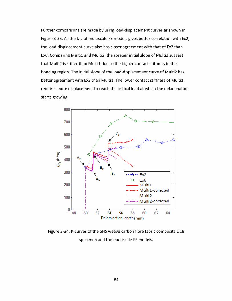
84
Further comparisons are made by using load-displacement curves as shown in
Figure 3-35. As the of multiscale FE models gives better correlation with Ex2,
the load-displacement curve also has closer agreement with that of Ex2 than
Ex6. Comparing Multi1 and Multi2, the steeper initial slope of Multi2 suggest
that Multi2 is stiffer than Multi1 due to the higher contact stiffness in the
bonding region. The initial slope of the load-displacement curve of Multi2 has
better agreement with Ex2 than Multi1. The lower contact stiffness of Multi1
requires more displacement to reach the critical load at which the delamination
starts growing.
Figure 3-34. R-curves of the 5HS weave carbon fibre fabric composite DCB
specimen and the multiscale FE models.

85
Although the raw value of Multi2 seems to be lower at point Cp, the
corrected is able to achieve slightly higher value than that of Ex2.
Considering the better correlation of Multi2 with Ex2, the result obtained by
Multi2 seems to be better representing the 5HS weave carbon fibre fabric
composite DCB specimen and the results of Multi2 is mainly analyzed.
Figure 3-35. Load-displacement curves of the 5HS weave carbon fibre fabric
composite DCB specimen and the multiscale FE models.
3.4.2 Energy released by CZM elements
Understanding the toughening mechanisms of 5HS weave carbon fibre fabric
composite DCB specimen is the main objective of this study. The energy release
rate obtained by experiments is based on the change of energy in global scale. FE
results, on the other hand, are able to provide alternative methods to quantify
the released energy. First, the released energy at delamination length is
defined by

86
(3.12)
where is the initial delamination length and is the critical energy release
rate. The released energy due to normal and tangential delamination can be
obtained by replacing by and , respectively.
The energy release rate is averaged over each element and multiplied by its area
to obtain the released energy. Figure 3-36 shows the released energies of Multi2
and 2D reference calculated by using the results of CZM elements and
calculated by MBT. The released energy of 2D reference calculated by MBT gives
almost identical value to that of calculated by CZM elements. This result is very
straight forward as only CZM elements release the energy due to delamination
growth.
On the other hand, the total released energy by CZM elements of Multi2 is
smaller than that obtained by MBT, i.e., global approach. This result indicates
that the multiscale DCB model were able to store more strain energy than 2D
homogeneous model for the same delamination length.
The total released energy by CZM elements consists of normal and tangential
components. seems to be very similar to that of 2D reference except slight
increase in the slope around delamination length 53mm. The increase seems to
be caused by the sub-surfaces that are created by lifting up weft yarn 2. For the
sake of analysis, the released energy is divided into three zones, i.e., Zone A
covering from the initial point to Point Ab, Zone B covering from Point Ab to Bb,
and Zone C covering from Point Bb to the ends. The delaminated elements at the
end of each zone are shown in Figure 3-37. The darker portions of the
delaminated area show multiple layers, i.e., sub-surfaces. The black portions
show the killed elements due to convergence difficulties. It is shown that sub-
surfaces appear in significant amounts from the end of Zone B and keep
increasing within Zone C. This result confirms the increase in the slope of . It

87
should be noted that there is sharp drop in the released energy due to the killed
elements during the solution. This drop should not be considered as any physical
phenomena.
The released energy by tangential debonding, i.e., , has as much as 14% of
total released energy as shown in Figure 3-38. As CZM elements are placed
around weft and warp yarns, there is always a portion of tangential debonding.
Figure 3-36. Released energies of the multiscale FE model of 5HS weave carbon
fibre fabric composite DCB and 2D plain-strain homogeneous FE model.

88
Figure 3-37. Delaminated areas at the end of each zone of the multiscale FE
model of 5HS weave carbon fibre fabric composite DCB.

89
Figure 3-38. Percentage of released energy by tangential debonding within the total released energy by CZM elements.
3.4.3 Toughening mechanisms
Although sub-surfaces and tangential debonding are indeed acting as toughening
compared to homogeneous model, that amount is not enough to explain the
difference in released energy calculated by MBT and CZM elements.
The toughening mechanism is discussed starting from Zone A to Zone C, which is
the same order as delamination growth. The toughening mechanism observed in
the multiscale FE model can be broken down to two mechanisms. The first
observed mechanism is the relaxation of stress concentration ahead of
delamination front caused by inter-yarns locking with the help of compressive
stresses ahead of delamination in DCB specimen. The deformation and stress
distribution of at Point Ap are shown in Figure 3-39. Unless otherwise noted,
the scaling factor for displaying the deformation is four. The compressive stress
ahead of delamination front, i.e., on weft yarn 2, is observed.

90
Figure 3-39. Contour plot of on the yarns at Point Ap and delaminated
elements coloured in pink.
The yarn interaction is rather easier to see with the contact pressure distribution
on the overlapping areas of yarns as shown in Figure 3-40. It indicates
compressive contact pressure, i.e., , against the yarns as positive value. As
compressive stresses exist in the warp and weft yarns at the ahead of
delamination front as shown in Figure 3-39, the overlapping areas experience
the compressive contact pressure . To understand the contributions from the
weave structure, the inter-yarn locking compressive contact pressure under in-
plane tensile loading at the same points are shown in Figure 3-41.
Delamination

91
Figure 3-40. Contour of contact pressure of the multiscale FE model and
delaminated elements (coloured in pink).
Figure 3-41. Contour of contact pressure of the meso-scale FE model under
in-plane tensile loading.
The meso-scale parts were taken from the multiscale DCB model with the initial
delaminations removed. Constant displacement is applied to the edge normal to
the x-direction. The magnitude of applied displacements is controlled to have
Delamination

92
the same range of contact pressure as that of multiscale DCB model. Figure 3-41
shows the upper warp and weft yarns for 2 plies only. The compressive contact
pressure indicates that inter-yarn locking exists on the overlapping areas where
the warp yarns change their paths to under and over the weft yarns. The
negative contact pressure, which is showing the stress to separate the yarns, is
also observed where the weft yarns are on the warp yarns. Figure 3-42 shows
the contact pressure at overlapping areas on line defined in Figure 3-41.
Contact pressures under two different magnitudes of in-plane tensile loading are
plotted with that of the multiscale DCB model. The contact pressure tendency of
in-plane loading is not very sensitive to the magnitude of applied load.
Accordingly, this tendency itself can be considered remain the same for the
multiscale DCB model at which some amount of exists. With this assumption,
the contact pressure of the multiscale DCB model at overlapping areas seems to
consist of relatively flat compressive pressure inherently caused by the DCB
specimen and pressure variations caused by yarn interactions. This implies that
there is inter-yarn locking effect in the multiscale DCB model ahead of
delamination front.
The effect of yarn interactions on the stress distribution near delamination front
at Point Ap is also investigated. Figure 3-43 shows the view of the upper warp
yarns, weft yarns, and matrix having positive clipped at from bottom
side. It is noted that the matrix near the overlap of warp yarn 3 and weft yarn 2
has positive indicating stress concentration due to delamination front is
slightly relaxed forward.
The stress distributions on lines defined in Figure 3-43 and contact pressures of
contact elements at under in-plane loading are plotted in Figure 3-44. The
minimum value of is observed on warp yarn 3 and its maximum value is
observed on warp yarn 1. The contact pressure, whose sign is reversed for sake
of better understanding, shows inter-yarn locking that may reduce the . The

93
overlap of weft yarn 1 and warp yarn 3 seems to have the highest reduction on
. It is noted, however, that the exact amount of reduction on by yarn
interaction cannot be obtained.
Figure 3-42. Contact pressure distribution on at Point Ap.

94
Figure 3-43. Contour plot of at Point Ap clipped at and delaminated
elements (coloured in pink).
By analyzing the results, it seems that inter-yarn locking caused by in-plane
deformation in the x-direction at the overlap of weft yarn 1 and warp yarn 3 and
the overlap of weft yarn 1 and warp yarn 4 has a toughening effect up to Point
Ap in addition to the toughening effect by inter-yarn locking of weft yarn 2 and
warp yarn 3. The contributions from the two toughening mechanisms cannot be
separated. However, the former toughening effect is smaller than latter because
the former toughening effect vanishes with delamination growth towards Point
Bp where the load reaches a higher value than that at Point Ap. The load drop
toward Point Ab seems be triggered by the delamination front under warp yarn 1
and weft yarn 1 because it has the highest stress compared to the others.
However, the delamination front seems to grow uniformly as shown Figure 3-45.
Delamination
Weft yarn 2
Warp yarn 3

95
Figure 3-44. near delamination front at Point Ap and reversed contact stress
obtained by in-plane loading.
Delamination

96
Figure 3-45. Delamination front development during the load drop from Point Ap
to Ab.
The toughening effect can be clearly explained by the stress distribution near
delamination tip at Point Ap. This approach, however, does not work well with
the case at Point Ab, which is the starting point of toughening toward Point Bp,
Ap
Ab

97
because the delamination has already been branched from the initial
delamination front. This makes the analysis difficult as shown in Figure 3-46.
Figure 3-46. The z-coordinates of delaminated elements showing the branching
at Point Ab.
On the other hand, the positive ahead of delamination front seems be an
alternative measurement of the stress relaxation at the delamination front. The
distance from the maximum delamination front at a given location in the y-
coordinate to the specified magnitude of ahead of the delamination front is
defined as as shown in Figure 3-47. is based on stress, which has been
divided into 9 color increments as shown in Figure 3-47, and represents the
difference in distance between zero stress (color red) and stress of 8MPa (color
blue). Figure 3-47 is at Point Ab where the delamination growth has just arrested.
The longest is obtained on warp yarn 3 up to 7MPa. This warp yarn 3 seems
to prevent delamination by inter-yarn locking with weft yarn 2. for =
1MPa shows the representative trend of over the width of the multiscale

98
DCB model as shown in Figure 3-48 for various points between Point Ab and Bb.
From Point Ab to Bp during which the load is increasing, has its highest values
on warp yarn 3. on warp yarn 3 is shortened during the transition from Point
Bp to Bb. This suggests that the inter-yarn locking resisted during the transition
from Point Ab to Bp, and is released as it goes toward Point Bb. This result seems
to support the toughening caused by the inter-yarn locking of warp yarn 3 and
weft yarn 2.
Figure 3-47. Length of positive from the delamination front at Point Ab.

99
The delaminated CZM elements from Point Ab to Bb are shown in Figure 3-49
with the warp and weft yarns of the upper ply as viewed from the bottom side.
Small amounts of delamination growth mainly on warp yarn 1 are observed
while the load increasing, i.e., Point Ab-Bp. This result suggests that warp yarn 1 is
not acting as the main source of toughening toward Point Bp because there is no
load drop due to the growth. By observing Figure 3-49, the delamination growth
on warp yarn 1 seems be a trigger for the entire delamination growth because
the delamination grows on warp yarn 1 first followed by the rest of yarns. Also,
on warp yarn 1 at Point Bp is relatively smaller than the rest of them as
shown in Figure 3-48. This implies the correlation between the likelihood of
delamination growth and .
At Point Bp- Bb, it is shown that delamination on warp yarn 1 and 2 goes intra-
ply, which is indicated by slightly darker areas because of transparent blue of
weft yarn 2, while the delamination on warp yarn 3 keeps going inter-ply. This
delamination growth pattern can be clearly seen at Point Bb. The exaggeratedly
scaled deformation of yarns at Point Bb is shown in Figure 3-50. The upper and
lower weft yarn 2, coloured in green and yellow, respectively, are bridging the
upper and lower plies. This bridging creates extra delamination surfaces which
are observed by X-rays [23] and are called sub-surfaces.
The inter-yarn locking ahead of delamination front played a significant role on
the toughening up to Point Bp. However, it does not seem to continue toward
Point Cp as weft yarn 3 has no crimping warp yarn. Accordingly, there is no
significant amount of inter-yarn locking effect expected ahead of delamination,
but the effect of weft yarn bridging gradually appeared from Point Bp.

100
Figure 3-48. distribution history from Point Ab to Bb.
The bridging effect reduces the stress concentration ahead of delamination front
if the weft yarns carry enough loads to resist. of the CZM element on the
delamination front edge at Point Bb is shown in Figure 3-51 with the z-coordinate
at the delamination front edge. The corresponding delaminated area is shown in
Figure 3-49, Bb. The values of on the warp yarns are in the range of 60 to
70MPa. This distribution does not seem to show significant amount of stress
relaxation at the delamination front unlike that of Point Ap as shown in Figure
3-44. This confliction indicates that there is no evidence of stress relaxing due to
the weft yarn bridging.

101
Figure 3-49. Delaminated CZM elements from Point Ab to Bb.
Ab Ab- Bp
Bp Bp- Bb Bb
1
2
3
4 2
Numbering

102
Figure 3-50. Weft yarn bridging of Multi2 observed at Point Bb.
Figure 3-51. of CZM element on the delamination front edge with the
delamination front z-coordinates at Point Bb.
The other possible source of toughening is simply due to the creation of sub-
surfaces that increases the delaminated area. To investigate this effect, the
delamination area calculated by the mean delamination length multiplied by the

103
width, i.e., A1, and the total delaminated area of CZM elements, i.e., A2, are
obtained and shown in Figure 3-52 together with their linear curve fittings. The
figure shows that the actual delamination area is around twice that of the
dominant delamination area, i.e., A1. The global energy release rate contributed
by normal debonding of CZM elements can be expressed by
(3.13)
where and is the width of the multiscale DCB
model. The equation states that the global energy release rate due to normal
debonding can be obtained by multiplying the critical energy release rate of
epoxy matrix by the ratio of delamination area increase rate, i.e., the slope, with
respect to the width of the multiscale DCB model.
Figure 3-52. Delamination area of Multi2 versus delamination length.
Accordingly, the energy release rate by normal debonding of all CZM elements
could be 430N/m. The additional energy release rate due to tangential

104
debonding should be added. It has been already shown that the contribution of
tangential debonding to the released energy has up to 14% as discussed in
subsection 3.4.2. If so, the tangential debonding should contribute 70N/m. The
total energy release rate by all CZM elements should be 500N/m. On the other
hand, value of Multi2 calculated by MBT at Point Cp is 486N/m with the
correction. The total energy release rate by CZM elements is only 2.88% higher
than that of Multi2 obtained by MBT.
So far, Multi2 results have been analyzed, but Multi1 results are also available.
value of Multi1 has a similar trend to that of Multi2 up to Point Bb as shown in
Figure 3-34. However, Multi1 seems to have superior toughening towards Point
Cp. The analogous analysis approach is used to obtain delamination area increase
rate of Multi1. The corrected value of energy release rate at Point Cp of Multi1
obtained by MBT is 528N/m. The ratio of delamination area by CZM elements,
which is shown in Figure 3-53, with respect to the width of the multiscale DCB
model is 2.39. Assuming 14% of total energy release rate is contributed by local
tangential debonding, the increased amount of delamination area would raise
the energy release rate to 556N/m, which is 5.30% higher than that obtained by
MBT. Although there is a speculative correction to the end-edge effects, this
good correlation suggests that the main source of toughening seems be the
creation of sub-surfaces .

105
Figure 3-53. Delamination area of Multi1 versus delamination length.
The main difference between Multi1 and Multi2 is the contact stiffness that
connects the meso-scale parts to the homogenized parts. The weft yarn bridging
of Multi1 is shown in Figure 3-54. If the contact stiffness is the cause of this
difference, it implies that the transition from homogeneous parts to meso-scale
parts needs to be improved. Using a finer mesh in homogeneous model and
longer initial delamination within meso-scale parts would eliminate the effect of
the transition on the delamination growth.

106
Figure 3-54. Weft yarn bridging of Multi1 at Point Bb.
In summary, the toughening of 5HS weave fabric composite DCB model consists
of two different mechanisms; 1. Inter-yarn locking ahead of delamination front
causing stress relaxation, 2. Sub-surfaces created via the weft yarn bridging
providing additional resistance. One of the literatures [42] on the experimental
investigations on 5HS weave carbon fabric composite suggested conflicting
concluding remarks, i.e., the cause of toughening is the weft yarn, which is acting
as periodic obstacles for delamination growth. By analyzing the current results,
there is no evidence of weft yarns acting as obstacles. Moreover, the FE model
would likely cause delamination arrest by the weft yarn if they actually acted as
obstacles because delamination growth direction is restricted to the CZM
elements that are inserted. The toughening explanation in [42] is obtained by the
experiments results, which are intermittent data on the side edge of specimen
and delamination surfaces. This limited amount of information may blind other
source of toughening mechanisms.
On the other hand, the experiments indeed showed more variable information,
such as fibre breakage that suggests fibre bridging [22-23] and transverse cracks
within the weft yarn [23]. These types of damage are omitted in the FE model in

107
order to clarify the effect of meso-scale structure of 5HS weave fabric composite.
As the R-curves obtained by the multiscale FE mode are in good agreement with
lower bound of experiment results, adding the above mentioned damage
mechanism may provide a result reaching upper bound of experiment results.
3.5 Discussions
The multiscale 5HS weave carbon fibre fabric composite DCB model was
developed in order to understand the toughening mechanism and to provide
better way of using the R-curves obtained by experiments. The only damage
considered in the model is delamination within pre-defined locations of matrix,
the interface of yarns and matrix, and the interfaces of warp yarns and weft
yarns. The cohesive zone modelling elements are used with a bilinear cohesive
law with material properties of epoxy matrix. Accordingly, there is no
consideration of fibre-matrix interaction, transverse matrix cracks within yarns
or fibre breakages in the model.
R-curves obtained by the multiscale FE models are within the range of
experimental results, but they are closer to the lower bound. This result makes
sense because the multiscale FE model does not consider all possible energy
dissipation mechanisms. Although the multiscale FE models gave a good
agreement with the lower bound, it is not possible to conclude that the FE
models completely capture the delamination growth behaviour of the lower
bound. However, it indeed captures significant amount of toughening caused by
the fabric structure.
The numerical results showed two types of toughening mechanisms. One of
them is inter-yarn locking causing stress relaxation at delamination front. This
toughening mechanism explains why the energy release rate at the initial
delamination length, where no significant amount of yarn and/or fibre bridging

108
exists, is higher than that of epoxy matrix itself. In terms of the use of R-curves
for delamination growth analysis of composite structures, the direct use of R-
curves for the part where out-of-plane tensile stress is applied to propagate
delamination may overestimate the damage tolerance because the toughening is
assisted by the compressive stress that exists ahead of delamination front of DCB
specimen.
The other toughening mechanism is the creation of sub-surfaces via weft yarn
bridging which is observed after the delamination grew over weft yarn 2 entirely.
Since it requires that local delamination must be developed, applying R-curves
value at the plateau region to the model with initial delaminations may severely
overestimate the damage tolerance. One of the examples for this case is to
simulate the effect of imperfections, e.g., leftover film or other contaminations,
unintentionally caused during the manufacturing.
Also, the size of delamination width to which R-curves are applied should be at
least the same as the unit cell size because the size is the minimum requirement
for the complete toughening mechanism to exist.
Lastly, a suggestion could be given to improve the testing method to provide
better input to the FE model. As discussed, inter-yarn locking is enhanced by the
compressive stresses ahead of the delamination tip. This compressive stress is
inherent to the DCB specimen test. Accordingly, this compressive stress ahead of
the delamination tip, having the same degree of toughening as DCB specimen is
not guaranteed to occur in a practical applications. For example, a practical
application made of 5HS weave fabric composite shown in Figure 3-2 b)
experiences out-of-plane stress due to forces transferred by the bracket. Unlike
the DCB specimen, the structure should have more tensile out-of-plane stresses
than compressive stresses. An experimental method for Mode I fracture
toughness without compressive stresses ahead of delamination tip is needed.

109
3.6 Future work
Understanding of toughening mechanism of 5HS weave fabric composites is the
objective of this study in order to have a better idea for R-curve usage for the
delamination growth simulation of composite structures. The results of this
study show two types of toughening mechanisms, but the mixture of the two
toughening mechanisms was not clearly observed due to the limitation on the
problem size. The multiscale 5HS weave fabric composite DCB model with
minimum width of a unit-cell, and larger meso-scale parts should be solved by an
analogous way. Also, it would be interesting to see the effect of various factors,
e.g., voids, weave fabric ply alignment, fibre volume fraction, type of weave
fabric, etc. Even though better understanding of the effect various factors would
bring more information to judge the proper usage of R-curves, all possible
combinations of simulations are not necessary because the experimentally
obtained R-curves have the properties of the weave fabric ply alignment, voids,
fibre volume fraction and type of weave fabric.
From this study, a minimum of unit cell size is recommended for the use of R-
curves. However, this size may be too large to capture local delamination
behaviour for some composite structures. In order to overcome this difficulty,
the R-curves need to be decomposed into a scale that is the same as the weft
and warp yarn width.
As inter-yarn locking is partially assisted by the compressive stress ahead of
delamination front, the effect of magnitude of out-of-plane compressive stress
should also be investigated. By knowing this effect, the R-curves would be
applied to the region where out-of-plane tensile stress is dominant ahead of
delamination front.
It is also worthwhile to focus on the mechanical toughening due to the woven
structure. The analysis shows that the woven structure doubled the fracture
toughness of matrix. In order to reveal the mechanisms of toughening due to the

110
woven structure, a similar procedure to what is provided in this thesis may be
used.
Most importantly, better numerical techniques for modelling delamination
growth are needed to be developed in order to save on computational time and
increase the accuracy of the simulation results.
4 Concluding remarks The industry’s demand for an efficient and accurate numerical simulation
method for analyzing damage behaviour of composite structures is high. This
study contributes to the demand by introducing a new crack modelling method
and by providing more information to understand damage mechanisms of 5HS
weave fabric composite laminates during delamination growth.
In Chapter 2, the proposed crack modelling method, which is called ADD-FEM,
successfully showed the delamination growth simulation capability and accuracy
by a 2D plane strain DCB specimen model. As ADD-FEM does not require the pre-
location of delamination path by inserting interface/contact elements, it is then
very useful. Also, no additional degrees of freedom are necessary to model
newly created delamination surfaces. This is a unique feature of ADD-FEM
compared to other methods that are capable of delamination growth simulation
with comparable accuracy.
In Chapter 3, the damage mechanism of 5HS weave composite was investigated
by applying multi-scale modelling techniques. The DCB model used to investigate
the damage mechanism has meso-scale parts, which consist of individually
modeled weft and warp yarns where the gaps are filled with epoxy matrix. These
meso-scale parts are bonded with homogeneous parts, which are used to model
the region where no damage is expected. To validate the model, R-curves and
Load-displacement curves of experiments and simulations are compared. The
simulation result showed better agreement with lower bound of experimental

111
results than upper bound. The previously undiscovered source of the toughening
mechanism was found by the meso-scale analysis. Although a meso-scale
analysis is not very efficient to model at the structural application level, the
extensive information obtained from the meso-scale analysis at the coupon scale
certainly benefits development of damage analysis at the structure scale.
Although future work is necessary in order to satisfy practical industrial needs,
the study puts forward the development of efficient and accurate damage
prediction capabilities under static loading.
4.1 Contributions of this thesis
The contributions of this thesis are listed as follows.
1) The crack modelling method called ADD-FEM provides an alternative method
for modelling strong discontinuity within an element without additional
degrees-of-freedom.
2) The multiscale analyses of a 5-harness satin weave carbon fibre composite DCB
specimen proved the usefulness of cohesive zone modelling for analyzing
complex crack growth within woven composite materials.
3) A previously unknown toughening mechanism in mode I delamination of 5-
harness satin weave carbon fibre composite was revealed by the multiscale
analyses. The analyses also confirmed that experimentally observed sub-
surfaces are the main source of toughening in mode I delamination.
4) The multiscale analysis results provided insight on the use of R-curves obtained
by mode I DCB tests.

112
4.2 Future work
In order to develop an efficient and accurate damage prediction capability under
static and fatigue loadings, there is still a lot of work to be done. Here is a list of
ideas that could be done as a direct extension of the work presented in this
thesis.
1) 3D formulation of ADD-FEM for a 8-node brick element could be derived. The
3D formulation would be necessary for crack modelling in 3D applications.
2) Formulations of ADD-FEM for higher order elements could be useful, but the
constraint equations for the mid-nodes must be newly developed. These
formulations would extend the usage of ADD-FEM.
3) Formulations of ADD-FEM should be verified with various shapes of sub-
elements, e.g., triangle, hexagonal etc. These formulations would add more
flexibility of the crack growth path.
4) Other types of woven fabric composite and other reinforcing fibres in the woven
fabric composite could be analyzed by a similar multiscale finite element model.
Further analyses on various types of woven composite would confirm whether
or not the toughening mechanism revealed by this study is unique to this
particular composite.
5) The multiscale model used in this study was halved in width and shortened the
length extensively due to the limitations of available computational resources.
The full scale model of the DCB specimen would provide better correlation with
the compatible experimental results.
6) The meso-scale parts of the multiscale model could possibly be used to analyze
mode II and mixed-mode delamination DCB tests.
7) The damage within fibre bundle was ignored in this study due to simplification.
Adding a cohesive zone model within fibre bundle will increase the required
computational resources, but it would also give better representation of actual
woven fibre composite. With the extra cohesive zone model, the model could
be used to analyze other types of tests, e.g., ultimate tensile strength test,
ultimate compressive strength test, etc.

113
References
1. Kensche, C.W., Fatigue of composites for wind turbines. International
Journal of Fatigue, 2006. 28(10): p. 1363-1374.
2. Kong, C., T. Kim, D. Han, and Y. Sugiyama, Investigation of fatigue life for
a medium scale composite wind turbine blade. International Journal of
Fatigue, 2006. 28(10): p. 1382-1388.
3. Shokrieh, M.M. and R. Rafiee, Simulation of fatigue failure in a full
composite wind turbine blade. Composite Structures, 2006. 74(3): p. 332-
342.
4. Marín, J.C., A. Barroso, F. París, and J. Cañas, Study of fatigue damage in
wind turbine blades. Engineering Failure Analysis, 2009. 16(2): p. 656-668.
5. Savage, G., Failure prevention in bonded joints on primary load bearing
structures. Engineering Failure Analysis, 2007. 14(2): p. 321-348.
6. Savage, G., Sub-critical crack growth in highly stressed formula 1 race car
composite suspension components. Engineering Failure Analysis, 2009.
16(2): p. 608-617.
7. Marsh, G., Airframers exploit composites in battle for supremacy.
Reinforced Plastics, 2005. 49(3): p. 26-32.
8. Marsh, G., Boeing's 787: Trials, tribulations, and restoring the dream.
Reinforced Plastics. 53(8): p. 16-21.
9. Msc nastran 2007 r1 implicit nonlinear (sol 600) user's guide: 2009.
10. Cavatorta, M.P., D.S. Paolino, L. Peroni, and M. Rodino, A finite element
simulation and experimental validation of a composite bolted joint loaded
in bending and torsion. Composites Part A: Applied Science and
Manufacturing, 2007. 38(4): p. 1251-1261.
11. Times, T.S. Boeing 787 wing flaw extends inside plane. 2009.
12. Mirzadeh, F. and K.L. Reifsnider, Micro-deformations in c3000/pmr15
woven composite. Journal of Composite Materials, 1992. 26(2): p. 185-
205.

114
13. ANSYS, I., Ansys help. 2009.
14. Wimmer, G., W. Kitzmüller, G. Pinter, T. Wettemann, and H.E.
Pettermann, Computational and experimental investigation of
delamination in l-shaped laminated composite components. Engineering
Fracture Mechanics, 2009. 76(18): p. 2810-2820.
15. Riccio, A., M. Giordano, and M. Zarrelli, A linear numerical approach to
simulate the delamination growth initiation in stiffened composite panels.
Journal of Composite Materials, 2010. 44(15): p. 1841-1866.
16. Pietropaoli, E. and A. Riccio, On the robustness of finite element
procedures based on virtual crack closure technique and fail release
approach for delamination growth phenomena. Definition and
assessment of a novel methodology. Composites Science and Technology,
2010. 70(8): p. 1288-1300.
17. Fish, J. and Q. Yu, Computational mechanics of fatigue and life predictions
for composite materials and structures. Computer Methods in Applied
Mechanics and Engineering, 2002. 191(43): p. 4827-4849.
18. Muñoz, J.J., U. Galvanetto, and P. Robinson, On the numerical simulation
of fatigue driven delamination with interface elements. International
Journal of Fatigue, 2006. 28(10): p. 1136-1146.
19. Turon, A., J. Costa, P.P. Camanho, and C.G. Dávila, Simulation of
delamination in composites under high-cycle fatigue. Composites Part A:
Applied Science and Manufacturing, 2007. 38(11): p. 2270-2282.
20. Harper, P.W. and S.R. Hallett, A fatigue degradation law for cohesive
interface elements - development and application to composite materials.
International Journal of Fatigue, 2010. 32(11): p. 1774-1787.
21. May, M. and S.R. Hallett, A combined model for initiation and
propagation of damage under fatigue loading for cohesive interface
elements. Composites Part A: Applied Science and Manufacturing, 2010.
41(12): p. 1787-1796

115
22. Feret, V., Development of a mixed-mode fracture criterion for a fabric
composite manufactured by rtm, master of engineering thesis, in
Department of Mechanical Engineering. 2009, McGill University:
Montreal.
23. Gill, A.F., P. Robinson, and S. Pinho, Effect of variation in fibre volume
fraction on modes i and ii delamination behaviour of 5hs woven
composites manufactured by rtm. Composites Science and Technology,
2009. 69(14): p. 2368-2375.
24. Turon, A., C.G. Dávila, P.P. Camanho, and J. Costa, An engineering
solution for mesh size effects in the simulation of delamination using
cohesive zone models. Engineering Fracture Mechanics, 2007. 74(10): p.
1665-1682.
25. Belytschko, T. and T. Black, Elastic crack growth in finite elements with
minimal remeshing. International Journal for Numerical Methods in
Engineering, 1999. 45(5): p. 601-620.
26. Moës, N., J. Dolbow, and T. Belytschko, A finite element method for crack
growth without remeshing. International Journal for Numerical Methods
in Engineering, 1999. 46(1): p. 131-150.
27. Oliver, J., Modelling strong discontinuities in solid mechanics via strain
softening constitutive equations. Part 1: Fundamentals. International
Journal for Numerical Methods in Engineering, 1996. 39(21): p. 3575-
3600.
28. Oliver, J., Modelling strong discontinuities in solid mechanics via strain
softening constitutive equations. Part 2: Numerical simulation.
International Journal for Numerical Methods in Engineering, 1996.
39(21): p. 3601-3623.
29. Linder, C. and F. Armero, Finite elements with embedded strong
discontinuities for the modeling of failure in solids. International Journal
for Numerical Methods in Engineering, 2007. 72(12): p. 1391-1433.

116
30. Liu, H., X.-L. Zhao, and R. Al-Mahaidi, Boundary element analysis of cfrp
reinforced steel plates. Composite Structures, 2009. 91(1): p. 74-83.
31. Mukherjee, S. and M. Morjaria, On the efficiency and accuracy of the
boundary element method and the finite element method. International
Journal for Numerical Methods in Engineering, 1984. 20(3): p. 515-522.
32. Bouchard, P.O., F. Bay, Y. Chastel, and I. Tovena, Crack propagation
modelling using an advanced remeshing technique. Computer Methods in
Applied Mechanics and Engineering, 2000. 189(3): p. 723-742.
33. Sheng Liu, Z. Kutlu, and F.-K. Chang, Matrix cracking and delamination in
laminated composite beams subjected to a transverse concentrated line
load. Journal of Composite Materials, 1993. 27(5): p. 436-470.
34. Rybicki, E.F. and M.F. Kanninen, A finite element calculation of stress
intensity factors by a modified crack closure integral. Engineering
Fracture Mechanics, 1977. 9(4): p. 931-938.
35. R. D. Cook, D.S.M., M. E. Plesha, Concepts and applications of finite
element analysis, third edition. 1989, New York: John Wiley & Sons.
36. Shephard, M.S., Linear multipoint constraints applied via transformation
as part of a direct stiffness assembly process. International Journal for
Numerical Methods in Engineering, 1984. 20(11): p. 2107-2112.
37. Sadd, M.H., Elasticity: Theory, applications, and numerics. 2005,
Burlington: Elesvier Butterworth-Heinemann.
38. Anderson, T.L., Fracture mechanics: Fundamentals and applications,
second edition. 1994, Boca Raton: CRC Press LLC.
39. Raju, I.S. and K.N. Shivakumar, An equivalent domain integral method in
the two-dimensional analysis of mixed mode crack problems. Engineering
Fracture Mechanics, 1990. 37(4): p. 707-725.
40. Chen, J.C., M. Kinloch, A.J. Busso, E.P. Matthews, F.L. Qiu, Y., Predicting
progressive delamination of composite material specimens via interface

117
elements. Mechanics of Composite Materials and Structures, 1999. 6: p.
301-317.
41. Roy, S., Mechanical modeeling and teting of a composite helicopter
structure made by resin transfer moulding, master of engineering thesis,
in Department of Mechanical Engineering. 2008, McGill University:
Montreal.
42. Alif, N., L.A. Carlsson, and L. Boogh, The effect of weave pattern and crack
propagation direction on mode i delamination resistance of woven glass
and carbon composites. Composites Part B: Engineering, 1998. 29(5): p.
603-611.
43. Yurgartis, S.W. and J.P. Maurer, Modelling weave and stacking
configuration effects on interlaminar shear stresses in fabric laminates.
Composites, 1993. 24(8): p. 651-658.
44. Bigaud, D. and P. Hamelin, Stiffness and failure modelling of 2d and 3d
textile-reinforced composites by means of imbricate-type elements
approaches. Computers & Structures, 2002. 80(27-30): p. 2253-2264.
45. Lee, C.S., S.W. Chung, H. Shin, and S.J. Kim, Virtual material
characterization of 3d orthogonal woven composite materials by large-
scale computing. Journal of Composite Materials, 2005. 39(10): p. 851-
863.
46. Iarve, E.V., D.H. Mollenhauer, E.G. Zhou, T. Breitzman, and T.J. Whitney,
Independent mesh method-based prediction of local and volume average
fields in textile composites. Composites Part A: Applied Science and
Manufacturing. 2009. 40(12): p.1880-1890.
47. Whitcomb, J.D., C.D. Chapman, and X. Tang, Derivation of boundary
conditions for micromechanics analyses of plain and satin weave
composites. Journal of Composite Materials, 2000. 34(9): p. 724-747.

118
48. Tang, X. and J.D. Whitcomb, General techniques for exploiting periodicity
and symmetries in micromechanics analysis of textile composites. Journal
of Composite Materials, 2003. 37(13): p. 1167-1189.
49. Xia, Z., Y. Zhang, and F. Ellyin, A unified periodical boundary conditions for
representative volume elements of composites and applications.
International Journal of Solids and Structures, 2003. 40(8): p. 1907-1921.
50. Xia, Z., C. Zhou, Q. Yong, and X. Wang, On selection of repeated unit cell
model and application of unified periodic boundary conditions in micro-
mechanical analysis of composites. International Journal of Solids and
Structures, 2006. 43(2): p. 266-278.
51. Woo, K. and J.D. Whitcomb, Effects of fiber tow misalignment on the
engineering properties of plain weave textile composites. Composite
Structures. 37(3-4): p. 343-355.
52. Karkkainen, R.L. and B.V. Sankar, A direct micromechanics method for
analysis of failure initiation of plain weave textile composites. Composites
Science and Technology, 2006. 66(1): p. 137-150.
53. Daggumati, S., W. Van Paepegem, J. Degrieck, J. Xu, S.V. Lomov, and I.
Verpoest, Local damage in a 5-harness satin weave composite under
static tension: Part ii - meso-fe modelling. Composites Science and
Technology, 2010. 70(13): p. 1934-1941.
54. Zako, M., Y. Uetsuji, and T. Kurashiki, Finite element analysis of damaged
woven fabric composite materials. Composites Science and Technology.
63(3-4): p. 507-516.
55. Tang, X. and J.D. Whitcomb, Progressive failure behaviors of 2d woven
composites. Journal of Composite Materials, 2003. 37(14): p. 1239-1259.
56. Lomov, S.V., D.S. Ivanov, I. Verpoest, M. Zako, T. Kurashiki, H. Nakai, and
S. Hirosawa, Meso-fe modelling of textile composites: Road map, data
flow and algorithms. Composites Science and Technology, 2007. 67(9): p.
1870-1891.

119
57. Key, C.T., S.C. Schumacher, and A.C. Hansen, Progressive failure modeling
of woven fabric composite materials using multicontinuum theory.
Composites Part B: Engineering, 2007. 38(2): p. 247-257.
58. Gorbatikh, L., D. Ivanov, S. Lomov, and I. Verpoest, On modelling of
damage evolution in textile composites on meso-level via property
degradation approach. Composites Part A: Applied Science and
Manufacturing, 2007. 38(12): p. 2433-2442.
59. Smilauer, V.t., C.G. Hoover, Z. P. Bazant, F.C. Caner, A. M. Waas, and K.W.
Shahwan, Multiscale simulation of fracture of braided composites via
repetitive unit cells. Engineering Fracture Mechanics. 2011. 78(6): p. 901-
918.
60. ASTM, D5528 standard test method for mode i interlaminar fracture
toughness of unidirectional fiber-reinforced polymer matrix composites.
2002.
61. Textile Composites Research, U.o.N.
Http://texgen.Sourceforge.Net/index.Php/main_page. 2010.
62. Composite Materials Group, K.U.L.
Http://sirius.Mtm.Kuleuven.Be/research/c2/poly/software.Html. 2010.
63. CYTEC, Cycom 890 rtm epoxy system. 2002.
64. Kaw, A.K., Mechanics of composite materials. 1997: CRC Press.

120
Appendix A
The selection of direction used in Eq. (2.5) requires a certain condition to
be met in order to obtain the constraint equations. , which is defined in
Eq. (2.7), is the derivative of shape functions with respect to which is
defined in the global coordinate system. Recall
(1.A)
According to the equation above, it is required that has a non-zero
value. Since the component of is the derivative of shape functions with
respect to , the first step is to obtain the derivative of shape functions with
respect to and , i.e.,
where
(2.A)
The derivative of the shape function with respect to is then given by
(3.A)
where is the unit vector in direction.
Then, is given by

121
(4.A)
where and are the components of unit vector in and ,
respectively. It should be noted that and are substituted into
only the derivatives of shape function in the right hand side of Eq. (4.A). The
condition to have can be obtained by
(5.A)
Therefore, the direction has to be chosen in such a way that
(6.A)
The identical condition can be obtained for
.

122
Appendix B
By using the assumption expressed by Eq. (2.5),
i.e.,
, and isolating gives
.
(1.B)
By using the assumption expressed by Eq. (2.5),
i.e.,
, and isolating gives
(2.B)
where is the component of the derivative operator matrix obtained for
the location of node 2 defined by Figure 2-3.
By using the assumption expressed by Eq. Figure 2-5,
i.e.,
, and isolating gives
(3.B)