i

DELAMINATION EFFECT ON RESPONSE OF A

COMPOSITE BEAM BY WAVELET SPECTRAL

FINITE ELEMENT METHOD

A THESIS SUBMITTED IN PARTIAL FULFILLMENT OF

REQUIREMENTS FOR THE DEGREE OF

MASTER OF TECHNOLOGY

IN

CIVIL ENGINEERING

BY

VENNA VENKATESWARAREDDY

210CE2030

Under the guidance of

DR. MANORANJAN BARIK

DEPARTMENT OF CIVIL ENGINEERING

NATIONAL INSTITUTE OF TECHNOLOGY, ROURKELA, ORISSA.

2012

ii

Dr. Manoranjan Barik

Associate Professor

Department of Civil Engineering

National Institute of Technology, Rourkela, Orissa, India. ---------------------------------------------------------------------------------------------------------------------

Certificate

This is to certify that the thesis entitled “DELAMINATION EFFECT ON RESPONSE OF A

COMPOSITE BEAM BY WAVELET SPECTRAL FINITE ELEMENT METHOD”

submitted by Mr. VENNA VENKATESWARAREDDY, bearing Roll No. 210CE2030 in

partial fulfilment of the requirements for the award of Master of Technology Degree in Civil

Engineering with specialization in Structural Engineering during 2010-2012 session at the

National Institute of Technology, Rourkela is an authentic work carried out by him under my

supervision.

To the best of my knowledge, the matter embodied in the thesis has not been submitted to any

other University/Institute for the award of any degree or diploma.

Rourkela Dr. Manoranjan Barik

Date: Associate Professor

Department of Civil Engineering

NIT Rourkela, 769008

iii

Acknowledgement

I am grateful to the Dept. of Civil Engineering, NIT ROURKELA, for giving me the

opportunity to execute this project, which is an integral part of the curriculum in M.Tech

programme at the National Institute of Technology, Rourkela.

I consider it my privilege to express my gratitude, respect and sincere thanks to all those

who guided and supported me in successful accomplishment of this project work. First of all I

would like to express my deepest sense of respect and indebtedness to my guide, Dr.

Manoranjan Barik, for his consistent support, guidance, encouragement, precious pieces of

advice in times, the freedom he provided and above all being nice to me round the year, starting

from the first day of my project work up to the successful completion of the thesis work.

My special thanks to Prof. N. Roy, Head of the Civil Engineering Department, for all the

facilities provided to successfully complete this work. I am also very thankful to all the faculty

members of the department, especially Structural Engineering specialization for their constant

encouragement, invaluable advice, encouragement, inspiration and blessings during the project.

The personal communication and discussion with Dr. Mira Mitra of Indian Institute of

Technology, Bombay is of immense help. Her valuable suggestions and timely co-operation

during the project work is highly acknowledged. The author extends his heartfelt thanks to her.

Especially I am thankful to my family members, all my classmates, friends and

Surendra Naga for their constant source of support, inspiration and valuable advices when in

need.

Venna Venkateswarareddy

iv

PREFACE

Transform methods are very useful to solve the ordinary and partial differential

equations. Fourier and Laplace transforms are the most commonly used transforms. Wavelet

transforms are most popular with electrical and communication engineers to analyse the signals.

From last few years, Wavelet transforms are in use for structural engineering problems, like

solution of ordinary and partial differential equations. Dynamical problems in structural

engineering fall under two categories, one involving low frequencies (structural dynamics

problems) and the other involving high frequencies (wave propagation problems).

Spectral Finite Element (SFE) method is a transform method to solve the high frequency

excitation problems which are encountered in structural engineering. SFE based on Fourier

transforms has high limitations in handling finite structures and boundary conditions. SFE based

with wavelet transforms is a very good tool to analyse the dynamical problems and eliminate

many limitations.

In this project, a model for embedded de-laminated composite beam is developed using

the wavelet based spectral finite element (WSFE) method for the de-lamination effect on

response using wave propagation analysis. The simulated responses are used as surrogate

experimental results for the inverse problem of detection of damage using wavelet filtering. The

technique used to model a structure that, through width de-lamination subdivides the beam into

base-laminates and sub-laminates along the line of de-lamination. The base-laminates and sub-

laminates are treated as structural waveguides and kinematics are enforced along the connecting

line. These waveguides are modeled as Timoshenko beams with elastic and inertial coupling and

the corresponding spectral elements have three degrees of freedom, namely axial, transverse and

v

shear displacements at each node. The internal spectral elements in the region of de-lamination

are assembled assuming constant cross sectional rotation and equilibrium at the interfaces

between the base-laminates and sub-laminates. Finally, the redundant internal spectral element

nodes are condensed out to form two-noded spectral elements with embedded de-lamination. The

response is being obtained by coding programs in MATLAB.

vi

CONTENTS

CHAPTER PAGE No.

CERTIFICATE………………………………………………………………………………...ii

ACKNOWLEDGEMENT…………………………………………………………………...iii

PREFACE………………………………………………………………………………………iv

CONTENTS…………………………………………………………………………………….vi

LIST OF FIGURES...................................................................................................................ix

LIST OF TABLES....................................................................................................................xii

ABBREVATIONS…………………………………………………………………………….xii

SYMBOLS……………………………………………………………………………………..xv

1 INTRODUCTION…………………………………………………………………...........1

1.1 Introduction …………………………………………………………………………...2

1.2 Solution methods for structural dynamic problems…………………………………...2

1.3 Solution methods for wave propagation problems…………………………………...4

2 LITERATURE REVIEW…………………………………………………………..........7

2.1 Natural frequency-based methods……………………………………………………..8

2.2 Mode shape-based methods………………………………………………………….12

2.3 Curvature/strain mode shape-based methods………………………………………...18

2.4 Other methods based on modal parameters………………………………………….20

vii

3 TRANSFORM METHODS…………………………………………………….............22

3.1 Laplace transforms…………………………………………………………………...23

3.2 Fourier transforms………………………………………………………………........25

3.2.1 Continuous Fourier transforms (CFT)…………………………………........25

3.2.2 Fourier Series (FS)…………………………………………………………..28

3.2.3 Discrete Fourier Transform (DFT)………………………………………….30

3.3 Wavelet transforms…………………………………………………………………...31

3.3.1 Types of wavelets…………………………………………………………...32

3.3.1.1 Morlet's Wavelet………………………………………………….32

3.3.1.2 Mexican Hat wavelet……………………………………………..34

3.3.1.3 The Continuous Wavelet Transform……………………………...34

3.3.1.4 Discrete Wavelet Transform………………………………….......35

3.3.2 Multi-resolution analysis………………………………………………........36

4 WAVELET INTEGRALS………………………………………………………...........39

4.1 Evaluation of wavelet integrals………………………………………………………..40

4.2 Construction of Daubechies compactly supported wavelets………………………....40

4.3 Scaling function and Wavelet function ………………………………......44

4.4 Connection Coefficients ( )………………………………………………………...49

4.5 Moment of scaling functions………………………………………………………….49

4.6 Impact load…………………………………………………………………………...52

viii

5 WAVELET BASED SPECTRAL FINITE ELEMENT FORMULATION…….53

5.1 Reduction of wave equations to ordinary differential equations…………………......54

5.1.1 Wavelet Extrapolation Technique…………………………………………….57

5.1.2 Calculation of wave numbers and wave amplitudes………………………….60

5.2 Spectral finite element formulation…………………………………………………..62

5.3 Modeling of de-lamination in composite beam………………………………………67

6 NUMERICAL EXAMPLES AND CONCLUSIONS…………………………….72

6.1 Wave responses to the impulse load………………………………………………….74

7 REFERENCES……………………………………………………………………...82-91

ix

LIST OF FIGURES

Figure 3.1: (a) Morlet's wavelet: real part………………………………………………………33

(b) Morlet's wavelet Imaginary part………………………………………………...33

Figure 3.2: Mexican Hat wavelet………………………………………………………………..34

Figure 4.1: (a) Scaling function for N=2………………………………………………………..45

(b) Wavelet function for N=2……………………………………………………...45

Figure 4.2: (a) Scaling function for N=4…………………………………………………….....46

(b) Wavelet function for N=4……………………………………………………...46

Figure 4.3: (a) Scaling function for N=12……………………………………………………...47

(b) Wavelet function for N=12…………………………………………………….47

Figure 4.4: (a) Scaling Function for N=22……………………………………………………..48

(b) Wavelet Function for N=22…………………………………………………....48

Figure 4.5: Discredited impulse time signal…………………………………………………….52

Figure 5.1: Composite beam element with nodal forces and nodal displacements……………..62

Figure 5.2: Graphite-Epoxy [0] 8layered cantilever beam ……………………………………..67

x

Figure 5.3: (a) Cross section at the end…………………………………………………………68

(b) Cross section at the de-lamination……………………………………………...68

Figure 5.4: Modeling of an embedded de-lamination with base and sub laminates……….........68

Figure 5.5: Representation of the base and sub base laminates by spectral elements…………..68

Figure 5.6: Force balance at the interface between base and sub laminate elements…………...69

Figure 6.1: Axial tip velocity of undamaged [ ] composite beam………………………...…..74

Figure 6.2: Transverse tip velocity of undamaged [ ] composite beam……………………….75

Figure 6.3: Axial tip velocities for undamaged and different de-lamination lengths

( =10mm and 20mm) along the centerline of [ ] layered composite beam……......76

Figure 6.4: Transverse tip velocities for undamaged and different de-lamination lengths

( =10mm and 20mm) along the centerline of [ ] layered composite beam……...76

Figure 6.5: Axial tip velocities for undamaged and different de-lamination lengths

( =30mm and 40mm) along the centerline of [ ] layered composite beam………77

Figure 6.6: Transverse tip velocities for undamaged and different de-lamination lengths

( =30mm and 40mm) along the centerline of [ ] layered composite beam………77

Figure 6.7: Axial tip velocities for undamaged and different position (0.25m and 0.35m)

of 20mm de-lamination from free end and along the centerline of [ ]

xi

layered composite beam…………………………………………………………….78

Figure 6.8: Transverse tip velocities for undamaged and different position (0.25m and 0.35m)

of 20mm de-lamination from free end and along the centerline of [ ]

composite beam……………………………………………………………………...78

Figure 6.9: Axial tip velocities for undamaged and different depths above the centerline

(h1=h, h1=h/2 and h1=h/4) of 20mm de-lamination of [ ] layered

composite beam……………………………………………………………………..79

Figure 6.10: Transverse tip velocities for undamaged and different depths above

the centerline (h1=h, h1=h/2 and h1=h/4) of 20mm de-lamination of [ ]

layered composite beam…………………………………………………………….80

Figure 6.11: Axial tip velocities for different orientation ( , , , and )

of 20mm de-lamination along the centerline of composite beam………………….80

Figure 6.12: Transverse tip velocities for different orientation ( , , , and )

of 20mm de-lamination along the centerline of composite beam…………………81

xii

LIST OF TABLES

Table 4.1: Filter Coefficients for N=22…………………………………………………………44

Table4. 2: First order (Ω1) and Second order (Ω

2) connection coefficients for N=22………….50

Table 4.3: Moment of Scaling Functions for N= 22…………………………………………….51

Table 6.1: Material properties of the Graphite- Epoxy composite beam……………………….73

xiii

ABBREVATIONS

ANN Artificial Neural Networks

AWCD Approximate Waveform Capacity Dimension

CFT Continuous Fourier Transform

CWT Continuous Wavelet Transform

DI Damage Index

DOF Degrees of Freedom

DST Discrete Fourier Transform

FD Fractal Dimension

FE Finite Element

FEM Finite Element Method

FFT Fast Fourier transform

FIR Finite Impulse Responce

FS Fourier Series

FSFE Fourier Transform based Spectral Finite Element

GFD Generalized Fractal Dimension

xiv

MDLAC Multiple Damage Location Assurance Criterion

MDOF Multi Degree of freedom

MRA Multiresolution Analysis

MSA Multiscale Analysis

MSC Mode Shape Curvature

NN Neural Network

ODE Ordinary Differential Equations

PDE Partial Differential Equations

PEP Polynomial Evaluation Problem

SCFEM Super Convergent Finite Element Method

SCCM Spectral Centre Correction Method

SDI Single Damage Indicator

SQP Sequential Quadratic Programming

SVD Singular Value Decomposition

SWT Stationary Wavelet Transform

ULS Uniform Load Surface

WSFEM Wavelet based Spectral Finite Element Method

xv

SYMBOLS

a Scaling parameter

Filter coefficients

In-plane laminate maduli coefficients

b Translation parameter

Width of the beam

In-plane/ flexure coupling laminate moduli coefficients

Constant coefficients

Approximation coefficients

d Rectangular pulse width

Detailed coefficients

Flexural laminate stiffness coefficient.

Young’s modulus of fibre along the longitudinal axis

Young’s modulus of fibre across the longitudinal axis

F(s) Function in terms of the Laplace s

F(t) Function in terms of time t

xvi

Nodal force vector of the element at node

Global Force vector

Shear modulus of composite in plane

2h Depth of the beam

Imaginary unit

Inertial constants

k Wave number.

Elemental Dynamic Stiffness Matrix

Global Dynamic Stiffness Matrix

L Length of the beam

Distance between the free end and edge of the de-lamination

De-lamination length

M Vanishing moment

Moment in spatial and temporal dimensions

Transformed moment

Number of sampling points

N Order of Debauchies

xvii

Transformed axial force

Axial force in spatial and temporal dimensions

[ ] Amplitude ratio matrix

and Transformation matrices

Time

Final time

Axial displacement in spatial and temporal dimensions

Nodal displacement vectors of the element at node

Global displacement matrix

Sequence of nested subspaces

Transverse force in spatial and temporal dimensions

Transformed transverse force

Transverse displacement in spatial and temporal dimensions

Thickness of each ply of laminate

pi

Circular frequency

Discrete circular frequency in

xviii

Scaling functions

Wavelet functions

Mother wavelet

First derivative of scaling function

Second derivative of scaling function

Direct sum

Orthogonal to each other

derivative of Connection coefficients

moment of scaling function

Time in micro second

Shear displacement in spatial and temporal dimensions

Mass density

First order connection coefficient matrix

Second order connection coefficient matrix

Eigenvector matrix of

Diagonal matrix containing corresponding eigenvalues

and Diagonal matrices

1

CHAPTER 1

INTRODUCTION

2

CHAPTER-1

INTRODUCTION

1.1 Introduction

Over the past few decades the composite materials are extensively used in many

engineering fields such as civil, mechanical and aerospace engineering etc. In-plane properties

of the composite material are much higher than its transverse tensile and inter-laminar shear

strength. Due to less strength in transverse direction composite structures are very much prone to

defects like matrix cracking, fibre fracture, fibre de-bonding, de-lamination/inter-laminar de-

bonding, of which de-lamination is most common, easily exposed to damage and it may increase,

thus reducing the life of the structure. Structural components are often subjected to damage

which can potentially reduce the safety. It is very important to find the weakest location and to

detect damage at the earliest possible stage to avoid brittle failure in future. This technique

(WSFEM) is based on the response-based approach since the response data are directly related to

damage. This approach is therefore fast and inexpensive.

1.2 Solution methods for structural dynamic problems

Generally dynamic analysis of the structure can be done by Finite Element Method

(FEM). In structural engineering, dynamic analysis of structures can be divided into two

categories, one is related with the low frequency loading categorized as structural dynamic

problems and another related with high frequency loading categorized as wave propagation

problems. Most of the structures of dynamic analysis come under structural dynamics. In

structural dynamics problems , the solution can be determined either by system parameters such

as natural frequencies and mode shapes or in terms of simulated response of the system to the

3

external excitation such as initial displacements support motion and applied load etc. The first

few mode shapes and natural frequencies are sufficient to analyze the performance of the

structure.

Finite Element solution of the dynamic analysis of the structure can be obtained by two

different methods [5] which are Modal Methods and Time Marching Schemes. In general, for

multi degree of freedom system (MDOF), the governing wave equation is coupled with a set of

ordinary differential equations (ODE). Linear transformation of the above ordinary differential

equations linearly and decoupled by modal matrix are referred as modal analysis. Modal

analysis is also an eigenvalue analysis and it is like one of the several numerical techniques such

as matrix iteration method. Simple continuous systems like rod, beam, plates can be solved

analytically. The solutions of such continuous systems are restricted though they are exact. But

complicated structures can be solved by approximate techniques. In general, approximate

techniques convert the continuous systems into discrete systems. These approximate techniques

are grouped into two categories. In the first group, the solution in terms of known functions are

assumed and they are combined linearly. For the continuous system, the governing differential

equations are partial differential equations. These partial differential equations are converted to a

set of ordinary differential equations by substituting the assumed solution with unknown

coefficient as variables. The Rayleigh-Ritz and Galerkin methods are the examples of this

method. In the other group, the dynamics of the continuous system is shown in terms of large

number of discrete points on the system. The finite element technique falls under this group. In

this finite element method the continuous structure is divided into number of elements and each

element connects through nodes surrounded by it. The continuous system of structure can be

reduced to multi degree of freedom system by expressing the dynamics in terms of the

4

displacements of the nodes. These displacements are approximated by some functions, the

coefficients of these functions are obtained in terms of the displacements of the nodes. This finite

element method can be applied to any arbitrary shapes and structure having high complexities.

Other methods such as boundary element method [7, 39] and meshless methods [6] and wave

finite element method [66]are applied for solving structural dynamic problems.

1.3 Solution methods for wave propagation problems

Multi modal problems are related with wave propagation analysis, in which the

extraction of eigenvalues is computationally most expensive. So Modal Methods are not suitable

for multi modal problems which are having very high frequencies. In the wave propagation

problems, the short term effects are critical, because the frequency of the input loading is very

high. To get the accurate mode shapes and natural frequencies, the wave length and mesh size

should be small. Alternatively we can use the time marching schemes under the finite element

environment. In this method, analysis is performed over a small time step, which is a fraction of

total time for which response histories are required. For some time marching schemes, a

constraint is placed on the time step, and this, coupled with very large mesh sizes, make the

solution of wave propagation problem. Wave propagation deals with loading of very high

frequency content and finite element (FE) formulation for such problems is computationally

prohibitive as it requires large system size to capture all the higher modes. These problems are

usually solved by assuming solution to the field variables say displacements such that the

assumed solution satisfies the governing wave equation as closely as possible. It is very difficult

to assume a solution in time domain to solve the governing wave equation. Therefore, ignore the

inertial part is ignored and the static part of the governing wave equation is solved exactly, and

this solution is used to obtain mass and stiffness matrices. This method of develop of finite

5

element is called Super Convergent Finite Element Method (SCFEM) [20, 9, 10, 42, 11]. This

method gives the smaller system size for wave propagation problems than conventional Finite

Element Method (FEM).

Alternatively, the solution in frequency domain is assumed and the governing equations

solve are transformed and solved exactly. This simplifies the problem by introducing the

frequency as a parameter which removes the time variable from the governing equations by

transforming to the frequency domain. Among these techniques, many methods are based on

integral transforms [22] which include Laplace transform, Fourier transform and most recently

wavelet transform. The solution of these transformed equations is much easier than the original

partial differential equations. The main advantage of this system is computational efficiency over

the finite element solution. These solutions in transformed frequency domain contain information

of several frequency dependent wave properties essential for the analysis. The time domain

solution is then obtained through inverse transform. In the frequency domain Fourier methods

can be used to achieve high accuracy in numerical differentiation. One such method is FFT based

spectral finite element method. The WSFE technique is very similar to the fast Fourier transform

(FFT) based spectral finite element (FSFE) except that it uses compactly supported Daubechies

scaling function approximation in time. In FSFEM, first the governing PDEs are transformed to

ODEs in spatial dimension using FFT in time. These ODEs are then usually solved exactly,

which are used as interpolating functions for FSFE formulation.

The advantages of FSFEM are, they reduces the system size and the wave characteristics

can be extracted directly from such formulation. The main drawback of FSFEM is that it cannot

handle waveguides of short lengths. This is because the required assumption of periodicity

results in wrap around problems, which totally distorts the response. It is in such cases,

6

compactly supported wavelets, which have localized basis functions can be efficiently used for

waveguides of short lengths. The wavelet based spectral finite element method follows an

approach very similar to FSFEM, except that Daubechies scaling functions are used for

approximation in time for reduction of PDEs to ODEs. The approach removes the problem

associated with ‘wrap around’ in FSFEM and thus requires a smaller time window for the same

problem. The Fourier transform is a tool widely used for many scientific purposes, but it is well

suited only to the study of stationary signals where all frequencies have an infinite coherence

time. The Fourier analysis brings only global information which is not sufficient to detect

compact patterns.

7

CHAPTER-2

LITERATURE REVIEW

8

CHAPTER-2

LITERATURE REVIEW

This review is organized by the classification using the features extracted for damage

identification, and these damage identification methods are categorized as follows:

1. Natural frequency-based methods;

2. Mode shape-based methods;

3. Curvature/strain mode shape-based methods;

4. Other methods based on modal parameters.

2.1 NATURAL FREQUENCY-BASED METHODS:- Natural frequency-based

methods use the natural frequency change as the basic feature for damage identification. The

choice of the natural frequency change is attractive because the natural frequencies can be

conveniently measured from just a few accessible points on the structure and are usually less

contaminated by experimental noise.

Liang et al. [36] developed a method based on three bending natural frequencies for the

detection of crack location and quantification of damage magnitude in a uniform beam under

simply supported or cantilever boundary conditions. The method involves representing crack as a

rotational spring and obtaining plots of its stiffness with crack location for any three natural

modes through the characteristic equation. The point of intersection of the three curves gives the

crack location and stiffness. The crack size is then computed using the standard relation between

stiffness and crack size based on fracture mechanics. This method had been extended to stepped

beams by Nandwana and Maiti [52] and to segmented beams by Chaudhari and Maiti [13]

using the Frobenius method to solve Euler-Bernoulli type differential equations.

9

Chinchalkar [14] used a finite element-based numerical approach to mimic the semi-analytical

approach using the Frobenius method. The beam is modelled using beam elements and the

inverse problem of finding the spring stiffness, given the natural frequency, is shown to be

related to the problem of a rank-one modification of an eigenvalue problem. This approach does

not require quadruple precision computation and is relatively easy to apply to different boundary

conditions. The results are compared with those from semi-analytical approaches. The biggest

advantage of this method is the generality in the approach; different boundary conditions and

variations in the depth of the beam can be easily modelled.

Morassi and Rollo [47] showed that the frequency sensitivity of a cracked beam-type structure

can be explicitly evaluated by using a general perturbation approach. Frequency sensitivity turns

to be proportional to the potential energy stored at the cracked cross section of the undamaged

beam. Moreover, the ratio of the frequency changes of two different modes turns to be a function

of damage location only. Morassi’s method based on Euler–Bernoulli beam theory modeled

crack and as a massless, infinitesimal rotational spring. The explicit expression is valid only for

small defects.

Kasper et al. [30] derived the explicit expressions of wave number shift and frequency shift for

a cracked symmetric uniform beam. These expressions apply to beams with both shallow and

deeper cracks. But the explicit expressions are based on high frequency approximation, and

therefore, they are generally inaccurate for the fundamental mode and for a crack located in a

boundary-near field.

Messina et al. [40] proposed a correlation coefficient termed the multiple damage location

assurance criterion (MDLAC) by introducing two methods of estimating the size of defects in a

structure. The method is based on the sensitivity of the frequency of each mode to damage in

10

each location. ‘MDLAC’ is defined as a statistical correlation between the analytical predictions

of the frequency changes f and the measured frequency changes f. The analytical frequency

change f can be written as a function of the damage extent vector D. The required damage

state is obtained by searching for the damage extent vector D which maximizes the MDLAC

value. Two algorithms (i.e., first and second order methods) were developed to estimate the

absolute damage extent. Both the numerical and experimental test results were presented to show

that the MDLAC approach offers the practical attraction of only requiring measurements of the

changes in a few of natural frequencies of the structure between the undamaged and damaged

states and provides good predictions of both the location and absolute size of damage at one or

more sites.

Lele and Maiti[34] extended Nandwana and Maiti’s method [53] to short beam, taking into

account the effects of shear deformation and rotational inertia through Timoshenko beam theory.

Patil and Maiti proposed a frequency shift-based method for detection of multiple open cracks in

an Euler–Bernoulli beam with varying boundary conditions. This method is based on the transfer

matrix method and extends the scope of the approximate method given by Liang for a single

segment beam to multi-segment beams. Murigendrappa et al. [50] later applied Patil and

Maiti’s approach to single/multiple crack detection in pipes filled with fluid.

Morassi [45] presented a single crack identification in a vibrating rod based on the knowledge

of the damage-induced shifts in a pair of natural frequencies. The analysis is based on an explicit

expression of the frequency sensitivity to damage and enables non uniform bars under general

boundary conditions to be considered. Some of the results are also valid for cracked beams in

bending. Morassi and Rollo [47] later extended the method to the identification of two cracks of

equal severity in a simply supported beam under flexural vibrations.

11

Kim and Stubbs [31] proposed a single damage indicator (SDI) method to locate and quantify a

crack in beam-type structures by using changes in a few natural frequencies. A crack location

model and a crack size model were formulated by relating fractional changes in modal energy to

changes in natural frequencies due to damage. In the crack location model, the measured

fractional change in the ith eigenvalue Zi and the theoretical (FEM based) modal sensitivity of the

ith

modal stiffness with respect to the jth element Fij is defined. The theoretical modal curvature is

obtained from a third order interpolation function of theoretical displacement mode shape. Then,

an error index eij is introduced to represent the localization error for the ith mode and the j

th

location. SDI is defined to indicate the damage location. While in the crack size model, the

damage inflicted aj at predefined locations can be predicted using the sensitivity equation. The

crack depth can be computed from aj and the crack size model based on fracture mechanics. The

feasibility and practicality of the crack detection scheme were evaluated by applying the

approach to the 16 test beams.

Zhong et al. [73] recently proposed a new approach based on auxiliary mass spatial probing

using the spectral centre correction method (SCCM), to provide a simple solution for damage

detection by just using the output-only time history of beam-like structures. A SCCM corrected

highly accurate natural frequency versus auxiliary mass location curve is plotted along with the

curves of its derivatives (up to third order) to detect the crack. However, only the FE verification

was provided to illustrate the method. Since it is not so easy to get a high resolution natural

frequency versus auxiliary mass location curve in experiment as in numerical simulation, the

applicability and practicality of the method in in-situ testing or even laboratory testing are still in

question.

12

Kim, B.H et al. [32] presented a vibration-based damage monitoring scheme to give warning of

the occurrence, location, and severity of damage under temperature induced uncertainty

conditions. A damage warning model is selected to statistically identify the occurrence of

damage by recognizing the patterns of damage driven changes in natural frequencies of the

structure and by distinguishing temperature-induced off-limits.

Jiang et al. [29] incorporated a tunable piezoelectric transducer circuitry into the structure to

enrich the modal frequency measurements, meanwhile implementing a high-order identification

algorithm to sufficiently utilize the enriched information. It is shown that the modal frequencies

can be greatly enriched by inductance tuning, which, together with the high-order identification

algorithm, leads to a fundamentally-improved performance on the identification of single and

multiple damages with the usage of only lower-order frequency measurements.

In 1997 Salawu [64] presented an extensive review of publications before 1997 dealing with the

detection of structural damage through frequency changes. In the conclusion of this review

paper, Salawu suggested that natural frequency changes alone may not be sufficient for a unique

identification of the location of structural damage because cracks associated with similar crack

lengths but at two different locations may cause the same amount of frequency change.

2.2 MODE SHAPE-BASED METHODS:-

Compared to using natural frequencies, the advantage of using mode shapes and their derivatives

as a basic feature for damage detection is quite obvious. First, mode shapes contain local

information, which makes them more sensitive to local damages and enables them to be used

directly in multiple damage detection. Second, the mode shapes are less sensitive to

environmental effects, such as temperature, than natural frequencies. The disadvantages are also

13

apparent. First, measurement of the mode shapes requires a series of sensors; second, the

measured mode shapes are more prone to noise contamination than natural frequencies.

Shi et al. [65] extended the damage localization method based on multiple damage location

assurance criterions (MDLAC) by using incomplete mode shape instead of modal frequency.

The two-step damage detection procedure is to preliminarily localize the damage sites by using

incomplete measured mode shapes and then to detect the damage site and its extent again by

using measured natural frequencies. No expansion of the incomplete measured mode shapes or

reduction of finite element model is required to match the finite-element model, and the

measured information can be used directly to localize damage sites. The method was

demonstrated in a simulated 2D planar truss model. Comparison showed that the proposed

method is more accurate and robust in damage localization with or without noise effect than the

original MDLAC method. In this method, the use of mode shape is only for preliminary damage

localization, and the accurate localization and quantification of damage still rely on measured

frequency changes.

Lee et al. [33] presented a neural network based technique for element-level damage

assessments of structures using the mode shape differences or ratios of intact and damaged

structures. The effectiveness and applicability of the proposed method using the mode shape

differences or ratios were demonstrated by two numerical example analyses on a simple beam

and a multi-girder bridge.

Hu and Afzal [28] proposed a statistical algorithm for damage detection in timber beam

structures using difference of the mode shapes before and after damage. The different severities

of damage, damage locations, and damage counts were simulated by removing mass from intact

14

beams to verify the algorithm. The results showed that the algorithm is reliable for the detection

of local damage under different severities, locations, and counts.

Pawar et al. [54] investigated the effect of damage on beams with clamped boundary conditions

using Fourier analysis of mode shapes in the spatial domain. The damaged mode shapes were

expanded using a spatial Fourier series, and a damage index (DI) in the form of a vector of

Fourier coefficients was formulated. A neural network (NN) was trained to detect the damage

location and size using Fourier coefficients as input. Numerical studies showed that damage

detection using Fourier coefficients and neural networks has the capability to detect the location

and damage size accurately. However, the use of this method is limited to beams with clamped-

clamped boundary condition.

Abdo and Hori [2] suggested that the rotation (i.e., the first derivative of displacement) of mode

shape is a sensitive indicator of damage. Based on a finite element analysis of a damaged

cantilevered plate and a damaged simply-supported plate, the rotation of mode shape is shown to

have better performance of multiple damage localization than the displacement mode shape

itself.

Hadjileontiadis et al. [24] and Hadjileontiadis and Douka [25] proposed a response-based

damage detection algorithm for beams and plates using Fractal Dimension (FD). This method

calculates the localized FD of the fundamental mode shape directly. The damage features are

established by employing a sliding window of length M across the mode shape and estimating

the FD at each position for the regional mode shape inside the window. Damage location and

size are determined by a peak on the FD curve indicating the local irregularity of the

fundamental mode shape introduced by the damage. If the higher mode shapes were considered,

this method might give misleading information as demonstrated in their study.

15

Wang and Qiao [69] proposed a modified FD method termed ‘generalized fractal dimension

(GFD)’ method by introducing a scale factor S in the FD algorithm, Instead of directly applying

the algorithm to the fundamental mode shape, the GFD is applied to the ‘uniform load surface’

(ULS) to detect the damage. Three different types of damage in laminated composite beams have

been successfully detected by the GFD. It should be pointed out that the GFD bears no

conventional physical meaning as compared to the FD, and it only serves as an indicator of

damage. A scale factor S has to be carefully chosen in order to detect damage successfully.

Qiao and Cao [58] proposed a novel waveform fractal dimension-based damage identification

algorithm. An approximate waveform capacity dimension (AWCD) was formulated first, from

which an AWCD-based modal irregularity algorithm (AWCD-MAA) was systematically

established. Then, the basic characteristics of AWCD-MAA on irregularity detection of mode

shapes, e.g., crack localization, crack quantification, noise immunity, etc., were investigated

based on an analytical crack model of cantilever beams using linear elastic fracture mechanics.

In particular, from the perspective of isomorphism, a mathematical solution on the use of

applying waveform FD to higher mode shapes for crack identification was originally proposed,

from which the inherent deficiency of waveform FD to identify crack when implemented to

higher mode shapes is overcome. The applicability and effectiveness of the AWCD-MAA was

validated by an experimental program on damage identification of a cracked composite

cantilever beam using directly measured strain mode shape from smart piezoelectric sensors.

Hong et al. [27] showed that the continuous wavelet transform (CWT) of mode shape using a

Mexican hat wavelet is effective to estimate the Lipschitz exponent for damage detection of a

damaged beam. The magnitude of the Lipschitz exponent can be used as a useful indicator of the

16

damage extent. It was also proved in their work that the number of the vanishing moments of

wavelet should be at least 2 for crack detection in beams.

Douka et al. [17, 18] applied 1D symmetrical 4 wavelet transform on mode shape for crack

identification in beam and plate structures. The position of the crack is determined by the sudden

change in the wavelet coefficients. An intensity factor is also defined to estimate the depth of the

crack from the coefficients of the wavelet transform.

Zhong and Oyadiji [72] proposed a crack detection algorithm in symmetric beam-like structures

based on stationary wavelet transform (SWT) of mode shape data. Two sets of mode shape data,

which constitute two new signal series, are, respectively, obtained from the left half and

reconstructed right half of modal displacement data of a damaged simply supported beam. The

difference of the detail coefficients of the two new signal series was used for damage detection.

The method was verified using modal shape data generated by a finite element analysis of 36

damage cases of a simply supported beam with an artificial random noise of 5% SNR. The

effects of crack size, depth and location as well as the effects of sampling interval were

examined. The results show that all the cases can provide evidence of crack existence at the

correct location of the beam and that the proposed method can be recommended for

identification of small cracks as small as 4% crack ratio in real applications with measurement

noise present. However, there are two main disadvantages of this method. First, the use of this

method based on SWT requires fairly accurate estimates of the mode shapes. Second, the method

cannot tell the crack location from its mirror image location due to its inherent limitation.

Therefore, in applying the method, both the crack location predicted and its mirror image

location should be checked for the presence of a crack.

17

Chang and Chen [12] presented a spatial Gabor wavelet-based technique for damage detection

of a multiple cracked beam. Given natural frequencies and crack positions, the depths of the

cracks are then solved by an optimization process based on traditional characteristic equation.

Analysis and comparison showed that it can detect the cracks positions and depths and also has

high sensitivity to the crack depth, and the accuracy of this method is good. The limitation of this

method is very common in wavelet transform methods, that is, there are peaks near the

boundaries in the wavelet plot caused by discontinuity and the crack cannot be detected when the

crack is near the boundaries.

Cao and Qiao [15] proposed a novel wavelet transform technique (so called ‘integrated wavelet

transform’), which takes synergistic advantage of the SWT and the CWT, to improve the

robustness of irregularity analysis of mode shapes in damage detection. Two progressive wavelet

analysis steps are considered, in which the SWT-based multiresolution analysis (MRA) is first

employed to refine the retrieved mode shapes, followed by CWT-based multiscale analysis

(MSA) to magnify the effect of slight irregularity. The SWT-MRA is utilized to separate the

multi-component modal signal, eliminate random noise and regular interferences, and thus

extract purer damage information; while the CWT-MSA is employed to smoothen, differentiate

or suppress polynomials of mode shapes to magnify the effect of irregularity. The choice of the

optimal mother wavelet in damage detection is also elaborately discussed. The proposed

methodology is evaluated using the mode shape data from the numerical finite element analysis

and experimental testing of a cantilever beam with a through-width crack. The methodology

presented provides a robust and viable technique to identify minor damage in a relatively lower

signal-to-noise ratio environment.

18

2.3 CURVATURE/STRAIN MODE SHAPE-BASED METHODS:- It has been

shown by many researchers that the displacement mode shape itself is not very sensitive to small

damage, even with high density mode shape measurement. As an effort to enhance the sensitivity

of mode shape data to the damage, the mode shape curvature (MSC) is investigated as a

promising feature for damage identification.

Pandey et al. [53] suggested for the first time that the MSC, that is, the second derivatives of

mode shape, are highly sensitive to damage and can be used to localize it. The curvature mode

shapes are derived using a central difference approximation. Result showed that the difference of

curvature mode shapes from intact and damaged structure can be a good indicator of damage

location. It is also pointed out that for the higher modes, the difference in modal curvature shows

several peaks not only at the damage location but also at other positions, which may lead to a

false indication of damage. Hence, in order to reduce the possibility of a false alarm, only first

few low curvature mode shapes can be used for damage identification.

Abdel Wahab and De Roeck [1] investigated the accuracy of using the central difference

approximation to compute the MSC based on finite element analysis. The authors suggested that

a fine mesh is required to derive the modal curvature correctly for the higher modes and that the

first mode will provide the most reliable curvature in practical application due to the limited

number of sensors needed. Then, a damage indicator called ‘curvature damage factor’, which is

the average absolute difference in intact and damaged curvature mode shapes of all modes, is

introduced. The technique is further applied to a real structure, namely bridge Z24, to show its

effectiveness in multiple damage location.

Swamidas and Chen [68] performed a finite element-based modal analysis on a cantilever plate

with a small crack. It was found that the surface crack in the structure will affect most of the

19

modal parameters, such as the natural frequencies of the structure, amplitudes of the response

and mode shapes. Some of the most sensitive parameters are the difference of the strain mode

shapes and the local strain frequency response functions. By monitoring the changes in the local

strain frequency response functions and the difference between the strain mode shapes, the

location and severity of the crack that occurs in the structure can be determined.

Li et al. [35] presented a crack damage detection using a combination of natural frequencies and

strain mode shapes as input in artificial neural networks (ANN) for location and severity

prediction of crack damage in beam-like structures. In the experiment, several steel beams with

six distributed surface-bonded strain gauges and an accelerometer mounted at the tip were used

to obtain modal parameters such as resonant frequencies and strain mode shapes.

Amaravadi et al [4] proposed an orthogonal wavelet transform technique that operates on

curvature mode shape for enhancing the sensitivity and accuracy in damage location. First, the

curvature mode shape is calculated by central difference approximation from the displacement

mode shapes experimentally obtained from SLV. Then, a threshold wavelet map is constructed

for the curvature mode shape to detect the damage. The experimental results are reasonably

accurate.

Kim et al. [32] proposed a curvature mode shape-based damage identification method for beam-

like structures using wavelet transform. Using a small damage assumption and the Haar wavelet

transformation, a set of linear algebraic equations is given by damage mechanics. With the aid of

singular value decomposition, the singularities in the damage mechanism were discarded.

Finally, the desired DI was reconstructed using the pseudo-inverse solution. The performance of

the proposed method was compared with two existing NDE methods for an axially loaded beam

without any special knowledge about mass density and an applied axial force. The effect of

20

random noise on the performance was examined. The proposed method was verified by a finite

element model of a clamped-pinned pre-stressed concrete beam and by field test data on the I-40

Bridge over the RioGrande

Shi et al. [65] presented a damage localization method for beam, truss or frame type structures

based on the modal strain energy change. The MSEC at the element level is suggested as an

indicator for damage localization.

2.4 OTHER METHODS BASED ON MODAL PARAMETERS:-

Ren and De Roeck [60] proposed a damage identification technique from the finite element

model using frequencies and mode shape change. The element damage equations have been

established through the eigenvalue equations that characterize the dynamic behavior. Several

solution techniques are discussed and compared. The results show that the SVD-R method based

on the singular value decomposition (SVD) is most effective. The method has been verified by a

simple beam and a continuous beam numerical model with numbers of simulated damage

scenarios. The method is further verified by a laboratory experiment of a reinforced concrete

beam.

Wang and Qiao [69] developed a general order perturbation method involving multiple

perturbation parameters for eigenvalue problems with changes in the stiffness parameters. The

perturbation method is then used iteratively with an optimization method to identify the stiffness

parameters of structures. The generalized inverse method is used efficiently with the first order

perturbations, and the gradient and quasi-Newton methods are used with the higher order

perturbations.

Rahai et al. [59] presents a finite element-based approach for damage detection in structures

utilizing incomplete measured mode shapes and natural frequencies. Mode shapes of a structure

21

are characterized as a function of structural stiffness parameters. More equations were obtained

using elemental damage equation which requires complete mode shapes. This drawback is

resolved by presenting the mode shape equations and dividing the structural DOFs to measured

and unmeasured parts. The nonlinear optimization problem is then solved by the sequential

quadratic programming (SQP) algorithm. Monte Carlo simulation is applied to study the

sensitivity of this method to noise in measured modal displacements.

Hao and Xia [26] applied a genetic algorithm with real number encoding to minimize the

objective function, in which three criteria are considered: the frequency changes, the mode shape

changes, and a combination of the two. A laboratory tested cantilever beam and a frame structure

were used to verify the proposed technique. The algorithm did not require an accurate analytical

model and gave better damage detection results for the beam than the conventional optimization

method.

Ruotolo and Surace [63] utilized genetic algorithm to solve the optimization problem. The

objective function is formulated by introducing terms related to global damage and the dynamic

behavior of the structure, i.e., natural frequencies, mode shapes and modal curvature. The

damage assessment technique has been applied to both the simulated and experimental data

related to cantilevered steel beams, each one with a different damage scenario. It is demonstrated

that this method can detect the presence of damage and estimate both the crack positions and

sizes with satisfactory precision. The problems related to the tuning of the genetic search and to

the virgin state calibration of the model are also discussed.

22

CHAPTER-3

TRANSFORM METHODS

23

CHAPTER-3

TRANSFORM METHODS

3.1 LAPLACE TRANSFORMS

Laplace transforms provide a method for representing and analyzing linear systems using

algebraic methods. The application of Laplace Transform methods is particularly effective for

linear ODEs with constant coefficients, and for systems of such ODEs. To transform an ODE,

we need the appropriate initial values of the function involved and initial values of its

derivatives. In systems that begin undeflected and at rest the Laplace‘s’ can directly replace the

d/dt operator in differential equations [70]. It is a superset of the phasor representation in that it

has both a complex part, for the steady state response, but also a real part, representing the

transient part. As with the other representations the Laplace “s” is related to the rate of change in

the system.

where,

F(s)= the function in terms of the Laplace s

F(t)= the function in terms of time t

The normal convention is to show the function of time with a lower case letter, while the same

function in the s-domain is shown in upper case. Another useful observation is that the transform

starts at s.The Laplace method is particularly advantageous for input terms that are

piecewise defined, periodic or impulsive.

24

Properties of Laplace transform:

1. Linearity:

2. First derivative:

3. Second derivative:

4. Higher order derivative:

5.

where this also implies

6.

where this implies

The original time signal can be obtained through an inverse transform of and is

written as

if

Let us consider for the Laplace transform is

This transform can be performed only analytically and there is no numerical implementation.

This restricts the use of Laplace transform for analysis of problems with higher complexities,

which need to be solved numerically.

25

3.2 FOURIER TRANSFORMS

The Fourier transform is a tool, this can adopt easily and spread throughout system and it

is used in many fields of science as a mathematical or physical tool to alter a problem into one

that can be more easily solved. The Fourier transform, in essence, decomposes or separates a

waveform or function into sinusoids of different frequency which sum to the original waveform.

It identifies or distinguishes the different frequency sinusoids and their respective amplitudes.

The main advantage of Fourier transform in structural dynamics and wave propagation problems

is that several important characteristics of system can be obtained directly from the transformed

frequency domain method. Fourier transform can be implemented analytically, semi analytically

and numerically in the form of Continuous Fourier Transform (CFT), Fourier Series (FS) and

Discrete Fourier Transform (DST) respectively.

In Fourier analysis the complex exponential function is often used. We have by the

Euler formula

Hence, can be considered as complex sinusoid. In general a complex valued function has the

form of

here is the real part of the and is the imaginary part of the , and both

are real valued functions.

3.2.1 CONTINUOUS FOURIER TRANSFORMS

The both forward and inverse continuous Fourier transform of any time signal , generally

shown as transform pair, which are

26

where is the CFT of , is the angular frequency, is the complex number ( ).

should be complex and a plot of amplitude of this function against frequency will give the

spectral density of the time signal . As an example, consider a rectangular pulse width‘d’.

this function can be written as

Substitute the equation (3.12) in the equation (3.11) of , we get

Now, allow the pulse to propagate in the time domain by an amount of seconds, and this can

be written in mathematical form

Substitute the above equation (3.14) in equation (3.13), we get

The magnitude of the equations (3.13) and (3.15) are same. The second transform exists phase

information. The change of phase in frequency domain refers the propagation of signal in the

time domain. By using CFT, spread of the signal can be calculated in the time and frequency

domain.

27

Properties of CFT

(a) Linearity: Consider, two functions for the incident and reflected waves

respectively in time and are the constants. The Fourier Transform of a function

can be obtained as This expression can also be

written as The symbol represents the Fourier

Transform.

(b) Scaling: If multiply with some non zero constant to the time signal will become

The Continuous Fourier Transform of the signal can be written as

This represents that compression occurs in time domain results and

dilation occurs in frequency domain results. The amplitude however decreases to keep

the energy constant.

(c) Time shifting: A shift in the time signal by is manifested as a phase change in the

transformed frequency domain obtained through Continuous Fourier Transform. After

shifting the time the transform pair can be written as .

(d) Symmetric property of the CFT: The CFT of the time signal is in complex form,

split this complex form into real and imaginary parts by using equation (3.9). The real

and imaginary part of the CFT can be written as

The first integral is an even function and second is an odd function.

That is .

28

Consider a point on CFT say origin ( ), the transform on the right side of the origin

can be written as . Similarly on the left side can be written as

This origin point is called

Nyquist frequency and it is very important to determine the half of the total frequency

rang.

(e) Convolution: This property of the CFT is very useful for understanding the signal

processing aspects and it has great importance in wave propagation analysis. This

property can be obtained by multiplying two time signals each other.

Substitute the equation (3.11) in equation (3.18) for both these functions written as

The above equation (3.19) can also be written as

Conversely we can also write as

3.2.2 FOURIER SERIES

Fourier series is in between the Continuous Fourier Transform (CFT) and Discrete

Fourier Transform (DFT). The inverse transform is represented by a series while forward

29

transform is still in the integral form as in the CFT. i.e. out of both equations, one still needs the

mathematical description of the time signal to get the transforms.

The Fourier Series (FS) can be written as

where

The equation (3.22) and equation (3.23) are corresponding to the inverse transform and forward

transform of the CFT respectively. Where is the discrete representation of time signal, and it

introduces the periodicity of time signal. The equations (3.22) and (3.23) can be writing in terms

of complex exponentials as

where

, and the signal repeats after seconds due to enforced periodicity.

Now this time signal, can also be write in terms of fundamental frequency as

where the fundamental frequency

in radians per second or Hz.

Consider the rectangular time signal and substitute in equation (3.25), we get

30

3.2.3 DISCRETE FOURIER TRANSFORM

The transform pair of CFT requires mathematical description of the time signal and their

integration. Data of the time signals are obtained from experiments. Hence, what we require is

the numerical representation for the transform pair, which is called the Discrete Fourier

Transform (DFT). It is an alternative way of mathematical representation of CFT in terms of

summations. Here the ultimate aim is to replace the integral involved in computation of the

Fourier coefficient by summation for numerical implementation. Divide the time signal into

number of constant triangles. The height of the triangle is and width of the triangle is

.

From equation (3.15) we can observe that the continuous transform of the rectangle is a

function. Similarly in discrete system, idealizing the signal as rectangle. Therefore, the DFT of

the signal will be the summation of functions. Hence the second integral of equation

(3.25) can be written as

If is very small, the value of above equation (3.28) nearly equal to unity. Hence the forward

and inverse Discrete Fourier Transform (DFT) can be written as

31

Here, varies from

The DFT of a real function is symmetric about nyquist frequency as like in the case of CFT. One

side of DFT coefficients about nyquist frequency is the complex conjugate of the coefficients on

other side of it. Thus real points are transformed to

complex points. Nyquist frequency can

be calculated by using the following expression

3.3 WAVELET TRANSFORMS

The word wavelet has been derived from the French word. The equivalent French word ondelette

meaning "small wave" was used by Morlet and Grossmann [23, 48, 49] in the early 1980s. A

wavelet is a wave-like oscillation with an amplitude that starts out at zero, increases, and then

decreases back to zero. It can typically be visualized as a "brief oscillation" like one might see

recorded by a seismograph or heart monitor. Generally, wavelets are purposefully crafted to have

specific properties that make them useful for signal processing. Wavelets can be combined, using

a "shift, multiply and sum" technique called convolution, with portions of an unknown signal to

extract information from the unknown signal. Wavelets are defined by the wavelet

function ψ(t) (i.e. the mother wavelet) and scaling function φ(t) (also called father wavelet) in the

time domain. The wavelet function is in effect a band-pass filter and scaling it for each level

halves its bandwidth. This creates the problem that in order to cover the entire spectrum, an

infinite number of levels would be required. The scaling function filters the lowest level of the

transform and ensures all the spectrum is covered.

Since from the last few decades many researchers showing their interest for the development and

application wavelets in many fields. Some of the researchers include Morlet and Grossmann [23]

32

developed formulation for the Continuous Wavelet Transform, Meyer [41] and Mallt [38]

developed multi resolution analysis using wavelets, Daubechies [16] for proposal of orthogonal

compactly supported wavelets and Stromberg [67] for early works on discrete wavelet transform.

As a mathematical tool, wavelets can be used to extract information from many different kinds of

data of signals and images. Sets of wavelets are generally needed to analyze data fully. A set of

"complementary" wavelets will deconstruct data without gaps or overlap so that the

deconstruction process is mathematically reversible. Thus, sets of complementary wavelets are

useful in wavelet based compression/decompression algorithms where it is desirable to recover

the original information with minimal loss.

3.3.1 TYPES OF WAVELETS

We have several wavelet functions such as Morlet wavelets, Mexican hat wavelets, Mayer

wavelets, Shanon wavelets, Daubechies wavelets e.t.c., out of these wavelet functions Morlet

wavelets and Mexican hat wavelets are explained here, Daubechies wavelet function explained

in chapter 4.

3.3.1.1 MORLET'S WAVELET

The wavelet defined by Morlet is:

(3.32)

It is a complex wavelet which can be decomposed in two parts, one for the real part, and the

other for the imaginary part.

33

where is a constant. The admissibility condition is verified only if . Figure 1shows

the real part of the Morlet wavelet function and figure 2 shows the imaginary part of the Morlet

wavelet function.

Figure 3.1: (a) Morlet's wavelet: real part

Figure 3.1: (b) Morlet's wavelet Imaginary part

-8 -6 -4 -2 0 2 4 6 8-0.4

-0.3

-0.2

-0.1

0

0.1

0.2

0.3

0.4

0.5Complex Morlet wavelet cmor1.5-1

Real part

-8 -6 -4 -2 0 2 4 6 8-0.5

-0.4

-0.3

-0.2

-0.1

0

0.1

0.2

0.3

0.4

0.5

Imaginary part

34

3.3.1.2 MEXICAN HAT WAVELET

The Mexican hat defined by Murenzi is:

It is the second derivative of a Gaussian (see figure 2).

Figure 3.2: Mexican Hat wavelet.

3.3.1.3 THE CONTINUOUS WAVELET TRANSFORM

The Morlet-Grossmann definition of the continuous wavelet transform for a 1D signal

is:

-5 -4 -3 -2 -1 0 1 2 3 4 5-0.4

-0.2

0

0.2

0.4

0.6

0.8

1Mexican hat wavelet

35

where is the mother wavelet, a (>0) is the scaling parameter, it represents the frequency

content of the wavelet and b is the translation parameter, it represents the location of wavelet in

time. The basis function of the wavelet transform retains the time locality and frequency locality.

The transform is characterized by the following three properties:

1. It is a linear transformation,

2. It is covariant under translations:

3. It is covariant under dilations:

The last property makes the wavelet transform very suitable for analyzing hierarchical structures.

It is like a mathematical microscope with properties that do not depend on the magnification.

3.3.1.4 DISCRETE WAVELET TRANSFORM

The discrete wavelet transform (DWT) can be derived from this theorem if we process a

signal which has a cut-off frequency. A digital analysis is provided by the discretisation of

equation (3.34) with some simple considerations on the modification of the wavelet pattern by

dilation. Usually the wavelet function has no cut-off frequency and it is necessary to

suppress the values outside the frequency band in order to avoid aliasing effects. We can work in

Fourier space, computing the transform scale by scale. The number of elements for a scale can be

reduced, if the frequency bandwidth is also reduced. This is possible only for a wavelet which

also has a cut-off frequency. The decomposition proposed by Littlewood and Paley provides a

very nice illustration of the reduction of elements scale by scale. This decomposition is based on

an iterative dichotomy of the frequency band. The associated wavelet is well localized in Fourier

space where it allows a reasonable analysis to be made although not in the original space. The

36

search for a discrete transform which is well localized in both spaces leads to multiresolution

analysis.

3.3.2 MULTI-RESOLUTION ANALYSIS

In any discretised wavelet transform, there are only a finite number of wavelet coefficients for

each bounded rectangular region in the upper half plane. Still, each coefficient requires the

evaluation of an integral. To avoid this numerical complexity, one needs one auxiliary function,

the father wavelet . The sequence of nested subspaces plays an important role in the

construction of wavelet functions. These nested subspaces represent the multi resolution of

wavelet function in The closed subspaces for with the following properties,

1.

2.

3.

4. if and only if

These properties of subspaces are related with scaling relation. Thus, the embedded

subspaces essentially reduces the problem of obtaining

5. Each subspace is spanned by integers translates of a single function,

Based on the above properties multi resolution analysis, we can conclude that, first we need to

find the scaling function . Such that its integer translates are the

Riesz bases for the space . Similarly, will form a basis for the space . Thus,

37

From equation (3.37) and (3.38), we can conclude that . Therefore the basis function of

space can be write in terms of basis function as

where are filter coefficients. The equation (3.39) gives the scaling function for

the space . The basis function can be defined as

where are the dilation and translation indices respectively. In the above equation

represents the frequency content and represents the time in the analysis of time signal.

Let us consider the approximation of the function into the subspace by the scaling

function as

In the above equation (3.41), are the approximation coefficients and

Similarly the wavelet function and its translates are the Riesz basis for the

subspace , can be expressed in terms of basis functions for as

Where and form the Riesz basis for subspace can be written as

Let us consider the approximation of the function into the subspace by the wavelet

function as

38

Here, are called as detailed coefficients.

The next step is to obtain the closure subspace for the subspace and its orthogonal

compliment such that

where the symbol represents the direct sum. The above equation (3.45) shows that the

subspaces are orthogonal to each other and we can write expression for .

Using the above procedure, calculate the approximations of the at higher scale from the

approximations of lower scale.

39

CHAPTER-4

WAVELET INTEGRALS

40

CHAPTER-4

WAVELET INTEGRALS

4.1 EVALUATION OF WAVELET INTEGRALS

Many wavelet algorithms require the evaluation of integrals which involve combination of

wavelets, scaling functions and their derivatives. We collectively refer to such integrals as

wavelet integrals. There are a few instances in which wavelet integrals can be evaluated

analytically. The accuracy and efficiency of the technique used to compute the integrals will

have a significant impact on the wavelet performance of the wavelet algorithm. For instance

wavelet-based algorithms for solving differential equations typically lead to integrals involving

wavelets and their derivatives. Wavelet integrals[8] which are commonly encountered in

construction of Daubechies compactly supported wavelet algorithms:

(a) Filter coefficients,

(b) Wavelet and Scaling function coefficients,

(c) Moments of Wavelet and Scaling functions and

(d) Connection coefficients.

4.2 CONSTRUCTION OF DAUBECHIES COMPACTLY

SUPPORTED WAVELETS

For a wavelet with compact support, φ(t) can be considered finite in length and is equivalent to

the scaling filter g. An orthogonal wavelet is entirely defined by the scaling filter - a low-pass

41

finite impulse responce (FIR) filter of length 2N and sum 1. In biorthogonal wavelets, separate

decomposition and reconstruction filters are defined. For analysis with orthogonal wavelets the

high pass filter is calculated as the quadrature mirror filter of the low pass, and reconstruction

filters are the time reverse of the decomposition filters. Daubechies and Symlet wavelets can be

defined by the filter coefficients.

Conditions to calculate the filter coefficients:

1. For uniqueness, normalization is done by considering the area under the scaling function

to be unity,

The above equation leads to the following condition on the filter coefficients,

2. For Daubechies wavelets, the integer translates of scaling functions are orthogonal, i.e.,

where

This gives the condition on the filer coefficients as

42

The conditions given by equations (4.2) and (4.4) are not sufficient to get unique set of filter

coefficients. For an coefficient system,

equations can get from equations (4.2) and

(4.4), remaining

equations can get by imposing some conditions on the wavelet functions.

For Daubechies wavelets, assumed that the scaling functions represents exactly the polynomials

order . Where

Therefore the polynomial order as

The above polynomial is in expanded form, similar to the equation (3.42) for and can be

written as

Since are orthogonal to the translates of , taking inner product of equation (4.6) with

gives

Substitute the equation (4.5) in equation (4.7), we get

The above expression is valid for all values of . Where Consider

and all other gives

43

The above equation can be written in term of filter coefficients, we get

where M is the moment of wavelet function. The scaling functions are obtained by solving

recursively the dilation equation (4.2), (4.4) and (4.5). Which can be expanded for DN as,

Above equation can be written as the following equations,

(0) = a0 (0)

(1) = a0 (2) + a1 (1) + a2 (0)

(2) = a0 (4) + a1 (3) + a2 (2) + a3 (1) + a4 (0)

… … …

(N-2) = aN-3 (N-1) + aN-2 (N-2) + aN-1 (N-3)

(N-1) = aN-1 (N-1)

This can also be written in the matrix form,

The above equation possesses eigenvalue problem and can be solved to obtain as the

eigenvector. The matrix A is known as the filter coefficients and can be solved from

equations. Filter coefficients are given table for N=22. Where N is the order of Daubechies

wavelet. The function in the MATLAB wavelet toolbox gives the filter coefficients.

Table 1 shows the values of filter coefficients for N=22.

44

4.3 SCALING FUNCTION AND WAVELET FUNCTION

Scaling functions and wavelet functions can be calculate by using the following

equations,

where

The following figures are shows the scaling functions and wavelet functions for the

By observing these figures we can say that smoothness increases by

increasing order of Debauchies.

Table 4.1: Filter Coefficients for N=22

Filter Coefficients for N=22

0.0264377294333137 0.0443145095659574

0.203741535201907 0.0294734895982882

0.636254348460787 -0.0217291381089843

0.969707536626371 - 0.00472468792819149

0.582605597780612 0.00696983509023781

-0.229491852355296 -0.000436416206187889

-0.387820982791004 -0.00126292559260676

0.0933997381355307 0.000352354877907889

0.211866179836356 0.0000769884777628895

-0.0657325829045156 -0.0000489812643698126

-0.0939586317975106 6.35586363589251E-06

45

Figure 4.1(a): Scaling function for N=2.

Figure 4.1(b): Wavelet function for N=2.

-1 -0.5 0 0.5 10

0.2

0.4

0.6

0.8

1

1.2

1.4scaling function for N=2

-1 -0.5 0 0.5 1-1.5

-1

-0.5

0

0.5

1

1.5wavelet functions for N=2

46

Figure 4.2(a): Scaling function for N=4.

Figure 4.2(b): Wavelet function for N=4.

0 0.5 1 1.5 2 2.5 3-0.4

-0.2

0

0.2

0.4

0.6

0.8

1

1.2

1.4scaling function for N=4

0 0.5 1 1.5 2 2.5 3-1.5

-1

-0.5

0

0.5

1

1.5

2wavelet functions for N=4

47

Figure 4.3(a): Scaling function for N=12.

Figure 4.3(b): Wavelet function for N=12.

0 2 4 6 8 10 12-0.6

-0.4

-0.2

0

0.2

0.4

0.6

0.8

1

1.2scaling function for N=12

0 2 4 6 8 10 12-1.5

-1

-0.5

0

0.5

1

1.5wavelet functions for N=12

48

Figure 4.4(a): Scaling Function for N=22

Figure 4.4(b): Wavelet Function for N=22

0 5 10 15 20 25-0.5

0

0.5

1scaling function for N=22

0 5 10 15 20 25-1

-0.8

-0.6

-0.4

-0.2

0

0.2

0.4

0.6

0.8

1wavelet functions for N=22

49

4.4 CONNECTION COEFFICIENTS

Connection coefficients ( ) are integrals involving combination of wavelets and scaling

functions, their translates and their derivatives. They are frequently encountered during the

discretization of ordinary and partial differential equations. The classes of wavelets for which

connection coefficients are usually desired are those wavelets which are orthogonal, biorthogonal

and compact support. The evaluation of connection coefficients for orthogonal wavelets:

4.5 MOMENT OF SCALING FUNCTIONS

Let be the moment of scaling function

The moment of scaling functions are easily calculated by using the following three recursive

equations given in Amaratunga and Williams (1997) [3],

Always the zero-th moment, of is 1by the normalization of ,

50

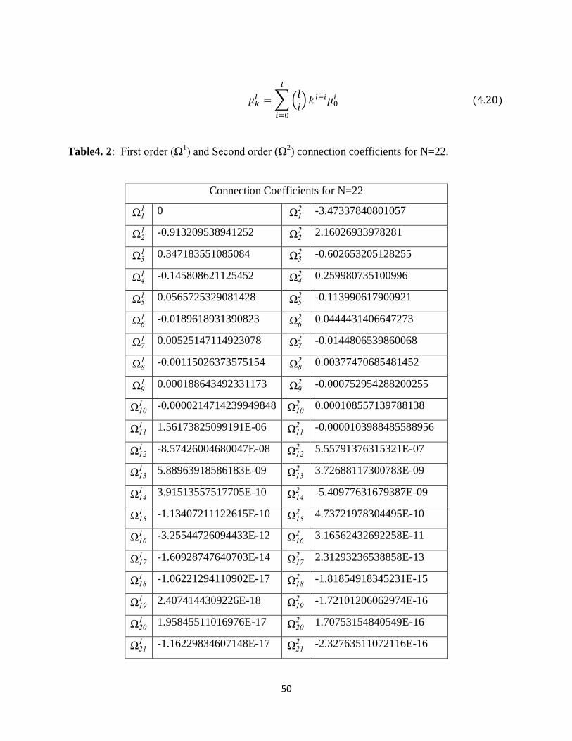
Table4. 2: First order (Ω1) and Second order (Ω

2) connection coefficients for N=22.

Connection Coefficients for N=22

0

-3.47337840801057

-0.913209538941252

2.16026933978281

0.347183551085084

-0.602653205128255

-0.145808621125452

0.259980735100996

0.0565725329081428

-0.113990617900921

-0.0189618931390823

0.0444431406647273

0.00525147114923078

-0.0144806539860068

-0.00115026373575154

0.00377470685481452

0.000188643492331173

-0.000752954288200255

-0.0000214714239949848

0.000108557139788138

1.56173825099191E-06

-0.0000103988485588956

-8.57426004680047E-08

5.55791376315321E-07

5.88963918586183E-09

3.72688117300783E-09

3.91513557517705E-10

-5.40977631679387E-09

-1.13407211122615E-10

4.73721978304495E-10

-3.25544726094433E-12

3.16562432692258E-11

-1.60928747640703E-14

2.31293236538858E-13

-1.06221294110902E-17

-1.81854918345231E-15

2.4074144309226E-18

-1.72101206062974E-16

1.95845511016976E-17

1.70753154840549E-16

-1.16229834607148E-17

-2.32763511072116E-16

51

Table 4.3: Moment of Scaling Functions for N= 22

Moment of Scaling Functions for N= 22

1

2.31726465941445

5.36971550177098

12.2319705607159

26.8773186714991

55.6323219714068

104.846598989408

169.689702637117

205.772899131726

92.0630949558087

-326.991286254096

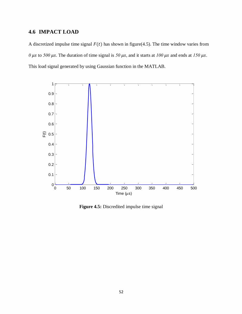
52

4.6 IMPACT LOAD

A discretized impulse time signal has shown in figure(4.5). The time window varies from

to The duration of time signal is and it starts at and ends at .

This load signal generated by using Gaussian function in the MATLAB.

Figure 4.5: Discredited impulse time signal

0 50 100 150 200 250 300 350 400 450 5000

0.1

0.2

0.3

0.4

0.5

0.6

0.7

0.8

0.9

1

Time (s)

F(t

)

53

CHAPTER-5

WAVELET BASED SPECTRAL FINITE

ELEMENT FORMULATION

54

CHAPTER 5

WAVELET BASED SPECTRAL FINITE ELEMENT FORMULATION

5.1 REDUCTION OF WAVE EQUATIONS TO ORDINARY DIFFERENTIAL

EQUATIONS

Governing wave equations for higher order composite beam [37] are,

where are the axial, transverses and shear displacements respectively.

where are the in-plane laminate maduli coefficients, in-plane/ flexure coupling

laminate moduli coefficients and flexural laminate stiffness coefficient. are the

inertial constants. These constants can be calculated by the following expression. is the mass

density , is the width of the beam and is the thickness of each ply of laminate. The force

boundary conditions associated with the governing differential equations are

55

where are the axial, transverse force and moment respectively. In

the formulation WSFE, reduce the governing differential equations (5.1)-(5.3) to ODE using

Daubechies scaling functions for approximation in time. The displacements

discredited at n points in the time window. Therefore the number of

sampling points the time at a particular instant can be obtained by

where is the time interval between two sampling points. Approximate the functions

and by scaling functions at an arbitrary scale as

Substitute above expressions in the governing wave equations we get

56

Taking inner product of on both sides of above equations with the translates of scaling functions

, and using their orthogonal properties, we get n simultaneous equations ordinary

differential equations are

where , is the order of the Daubechies wavelet and ,

are the

first and second order connection coefficients respectively.

For compactly supported wavelets these first and second order connection coefficients [8] are

non zeros at an interval of By observing the

equations(ODEs), the connection coefficients near the boundaries at lie

outside the time window [ ]. The falling of these connections coefficients outside the time

window will create problems with finite length data sequence. Therefore the coefficients at the

boundary need treatment. This treatment can be done using capacitance matrix and penalty

function methods [56,57]. To solve this boundary value problem, a wavelet based extrapolation

scheme proposed by Amaratunga and Williams(1997)[3,71] is used. This method is particularly

suitable for approximation time for the ease of imposition of initial conditions. The treatment of

57

boundaries for finite domain analysis can be done by using wavelet extrapolation technique. The

equation (5.11) can be written in matrix algebraic equations and can be solved by conventional

techniques. The equation (5.11) gives the algebraic coupled equations. are known in the

interval of time 0 to . Where varies from . Out of algebraic coupled equations,

some equations contain coefficients corresponding to to . This condition

shows that, the coefficients lie outside of the time window [0- ]. Similarly the same problem

exist on other boundary for to .

5.1.1 WAVELET EXTRAPOLATION TECHNIQUE

The coefficients of Daubechies scaling function has

vanishing moments, and that its

translates can be combined to give exact representation of polynomial order . Assume that

has a polynomial representation of order in the vicinity of the left boundary , we

have

where are constant coefficients. By taking inner product of equation (5.12) with on

both sides, we get

where are the moment of scaling functions defined in equation (4.17) and solving the

recursive equations in 4.4. Solve the equation (5.12) using finite difference scheme, we get

initial values of . Substitute these values in equation (5.13) and get the values in

58

terms of initial values. Like that the unknown coefficients on LHS can calculate by using the

following relation

1

1

0

1

2

1

2

0

2

1

2

1

2

0

2

1

1

1

1

0

1

2

2

1

pp

NNN

p

p

Nc

c

c

u

u

u

(521)

Similarly assume the polynomial representation to obtain the unknown coefficients at the

RHS as

The above equation (5.15) can be written in matrix form as

(5.23)

)1(

2)1(

1)1(

1

1

0

1

1

1

1

0

1

1

1

1

1

0

1

110

n

pn

pn

pp

p

ppp

p

ppp

u

u

u

c

c

c

calculate the values from the above equation (5.16), and substitute back in equation (5.15) for

, we get

(5.24)

1

1

0

1

2

1

2

0

2

1

1

1

1

0

1

1

0

1

0

0

0

21

1

pp

NNN

p

p

Nn

n

n

c

c

c

u

u

u

Finally, after getting the unknown coefficients on LHS and RHS, substitute these unknown

59

coefficients in equation (5.9), (5.10) and (5.11), and the system of coupled equations can be

written in matrix form as

where is the first order connection coefficient matrix obtain after using the wavelet

extrapolation technique. is the second order connection coefficient matrix[8] evaluated

independently, and this can also be written as . This modification of second order

connection coefficient matrix will helps in the imposition of initial conditions for non periodic

solutions[43]. The reduced ordinary differential equations (ODE) are coupled in wavelet spectral

finite element (WSFE). Decoupling of these equations can be done by eigenvalue analysis of

connection coefficient matrix and can be written as

Here is the eigen vector matrix of and is the diagonal matrix containing corresponding

eigenvalues . Similarly the eigenvalue analysis of second order connection coefficient

can be written as

Here, is a diagonal matrix with diagonal terms . These matrices and are

independents of the problem and depends only on the order of wavelet . After decoupling of

the equations (5.18),(5.19) and (5.20) can be written as

60

where and . Similarly the force boundary conditions

given by (5.6)-(5.8) can be written as

where and and are the transformed force boundary conditions of

and respectively.

5.1.2 CALCULATION OF WAVE NUMBERS AND WAVE AMPLITUDES

The parameters such as wave numbers and wave speeds are required to understand the wave

mechanics in the wave guide and these are required in SFE formulation to know the wave

characteristics like the wave mode is in propagating mode or damping mode or combination of

both. This spectral analysis starts with the partial differential equations (5.1)-(5.3) governing the

waveguide. and are the field variables in spatial and temporal

dimensions. These field variables are transformed to frequency domain by using DFT as

61

Here is the discrete circular frequency in , is the total number of frequency points

used in the transformation and , and are the DFT coefficients, varies with only. The

discrete circular frequency related with the time window as

where is the time sampling rate and is the highest frequency captured by decides the

frequency content of the load and considering the wrap around problem and decides the

aliasing problem [18]. Substitute the equations (5.36)-(5.38) in equations (5.1)-(5.3), we get

Assuming the solutions of above equations as ,

and .

Here and are the constants, later these can be derived from boundary values and k is the

wave number. Substituting these solutions in equations (5.39)-(5.41), we get

The above equations can also be write in matrix form, we get

62

These wave numbers k were obtained as a function of circular frequency , and computation of

wave numbers are very difficult for higher composite structures due to its coupling of transverse

and shear displacements and elastic coupling. In order to calculate the wave numbers and

associated wave amplitudes for such problems have been proposed by S. Gopalakrishnan [21].

Singular value decomposition (SVD) and polynomial evaluation problem (PEP) methods are

used to solve these problems. In this project, PEP method is used to solve the equation (5.42)-

(5.44) and those equations are written in the form PEP in k as

Here are the matrices, where is the number of independent variables in

the governing equations. Thus, the PEP is of the order . In this project, and .

The PEP for equation(5.45) is given as

where

By solving the equation (5.47)`using “polyeig” in the MATLAB, gives the eigenvalues and

eigenvectors. These eigenvalues represents the wavenumbers and eigenvectors represents the

corresponding wave amplitudes.

5.2 SPECTRAL FINITE ELEMENT FORMULATION

The equations (5.39) to (5.41) are solved exactly to get the shape functions in terms of some

unknown constants. These unknown constants are again solved in terms of boundary values and

these are useful in the formulation of elemental dynamic stiffness matrix of the transformed

nodal displacements with transformed nodal forces.

63

Figure 5.1: Composite beam element with nodal forces and nodal displacements

The above figure shows the beam element with three degrees of freedom such as , and

represents the axial, transverse and shear displacements at node1 and node2 respectively and

, and are the axial, transverse forces and moments at node1 and node2 respectively.

The transformed ODEs (5.30) to (5.32) are need to be solved for the , and and the actual

solutions , and are obtained from inverse wavelet transform and solve

these equations exactly, gives the exact shape functions (interpolating functions) which are

where L is the length of the element and and are the wave numbers corresponding to

the axial, transverse and shear modes of the element and explained in Mitra & Gopalakrishnan

(in press)

64

The above equations (5.48)-(5.50) can be written in matrix form as

161514131211 RRRRRR

262524232221 RRRRRR

363534333231 RRRRRR

)(ik-

ik-

)(ik-

ik-

)(ik-

3

3

2

2

1

1

e

e

e

e

e

xL

x

xL

x

xL

xike

6

5

4

3

2

1

c

c

c

c

c

c

Here is the nodal displacement vector of element at each node. [ ] is the amplitude

ratio matrix and this matrix can be obtained by solving the PEP equation (5.47). The solution of

equation (5.47) gives the eigenvalues and eigenvectors. [ ] is the eigenvector matrix and

eigenvalues are the wave numbers and . is the diagonal matrix with the

diagonal elements xike 1 )(-ik1e

xL x2-ike )(-ik2e

xL x3-ike )(-ik3e

xL and

are the unknown coefficients and these are obtained by applying the

boundary conditions at node 1 and node 2 as shown in figure 5.1.

Applying the boundary conditions at two nodes of element as shown in figure 5.1 to get

unknown constants in terms of nodal displacements. Put in equation (5.51), gives the

nodal displacements at node1, and the equation becomes

Put in equation (5.51), gives the nodal displacements at node2, and the equation becomes

65

Here

is the nodal displacement vector at node 1, similarly

is the nodal displacement vector at node 2. and are the diagonal matrices

and these are shown in the next page.

1

e

1

e

1

e

e

1

e

1

e

1

3

2

1

3

2

1

ik-

ik-

-ik

2

ik-

ik-

ik-

1

L

L

L

L

L

L

From equations (5.52) and (5.53), the nodal displacement vector

of an element

can be written as

where

and and similarly

.

The derivatives of the interpolating functions are given as

66

The above equations (5.55)-(5.57) can be written in matrix form as

6

5

4

3

2

1

)(ik-

ik-

)(ik-

ik-

)(ik-

363353342332321311

263253242232221211

163153142132121111

3

3

2

2

1

1

e

e

e

e

e

=

c

c

c

c

c

ce

RikRikRikRikRikRik

RikRikRikRikRikRik

RikRikRikRikRikRik

M

V

P

xL

x

xL

x

xL

xik

Here is the nodal force vector of element at each node. is the diagonal matrix with the

diagonal elements xike 1 )(-ik1e

xL x2-ike )(-ik2e

xL x3-ike )(-ik3e

xL and

are the unknown coefficients and these are obtained by applying the

boundary conditions at node 1 and node 2 as shown in figure 5.1.

Applying the boundary conditions at two nodes of element as shown in figure 5.1 to get

unknown constants in terms of nodal forces. Put in equation (5.58), gives the nodal

forces at node1, and the equation becomes

Put in equation (5.58), gives the nodal displacements at node2, and the equation becomes

Here

is the nodal force vector at node 1, similarly

is the

nodal force vector at node 2. and are the diagonal matrices as given above.

From equations (5.59) and (5.60), the nodal force vector

of an element can be

written as

67

where

and and similarly

.

From equation (5.54),

Substitute the equation (5.62) in equation (5.61) we get

The above equation can also be written as

where is the elemental dynamic stiffness matrix of size and this matrix is divided

into four sub matrices of size , and rewrite the equation (5.64) as

where and

are the nodal force and displacement vectors of the element at node.

5.3 MODELING OF DE-LAMINATION IN COMPOSITE BEAM

The modeling of embedded de-lamination of the composite beam is done according to the

method presented by Nag et al.[51]. The following figure 5.2 shows the embedded de-lamination

of the graphite – epoxy cantilevered beam.

68

where L is the length of the beam, is the distance between the free end and edge of the de-

lamination, is the de-lamination length, 2h is the depth of the beam and b is the width of the

beam. Figure 5.3(a) and 5.3(b) are shows the cross sections of the beam at the end and at the de-

laminated portion of the composite beam

Figure 5.3(a): Cross section at the end Figure 5.3(b): Cross section at the de-lamination

Figure 5.4: Modeling of an embedded de-lamination with base and sub laminates.

Figure 5.5: Representation of the base and sub base laminates by spectral elements.

Figure 5.2 shows the delaminated composite beam divided into four elements as shown in

Figure5.4, out of four elements element 1 and element 2 are called as base laminates and element

3 and element 4 are called as sub laminates. Every element of the beam is considered as

individual structural wave guides and modeled as coupled composite Timoshenko beam by using

WSFE method as discussed in previous section.

From equation (5.65), the nodal force vector for element 1is written as

69

Similarly, the nodal force vector for element 2 is written as

The kinematic assumption at the interfaces of the base and sub laminates is that the constant

cross sectional slope. From this assumption, the constant and continuous slope at the two

interfaces between base laminates and sub base laminates gives relation of nodal displacement

vector of sub laminates in term of base laminates.

Figure 5.6: Force balance at the interface between base and sub laminate elements.

From the above Figure, the nodal displacement vector at node 3 and node 5 is written in terms of

node 4 as

From the above expression and

can be written as

70

Similarly, the nodal displacement vector at node 6 and node 8 is written in terms of node 7 as

From the above expression and

can be written as

where represents the nodal displacement vector of element at node. and are the

transformation matrices in terms of top and bottom sub laminate thicknesses and .

From the force equilibrium equation at interface AB as shown in figure (5.5)

The equation (5.70) can be written as

Similarly, the force equilibrium equation at interface CD as shown in figure (5.5)

The equation (5.72) can be written as

The nodal force vector for element 3 is written as

71

Substitute and

values in equation (5.74) and pre-multiplying with on both sides, we get

Similarly, The nodal force vector for element 4 is written as

Substitute and

values in equation (5.76) and pre-multiplying with on both sides, we get

After calculation of elemental nodal force vectors, assemble the four spectral elements, we get

Nodal displacements at fixed end are zero i.e. at node 1, and nodal forces vectors are zero

at node 4 and node 7. Using these conditions, the equation (5.78) can be written as

where is the reconstructed dynamic stiffness matrix for the spectral element with embedded

de-lamination of cantilever composite beam.

72

CHAPTER 6

NUMERICAL EXAMPLES AND

CONCLUSIONS

73

CHAPTER 6

NUMERICAL EXAMPLES AND CONCLUSIONS

The wave propagation of the composite beam is obtained by using WSFE as discussed in the

previous chapter for broad band impulse load as shown in Figure (4.5). These numerical

experiments are done over an eight layered AS4/3501-6 graphite-epoxy composite beam. The

properties of AS4/3501-6 graphite-epoxy composite beam are given in the following table 6.1.

Table 6.1: Material properties of the Graphite- Epoxy composite beam:

Material properties

141.90 Gpa.

9.78 Gpa.

6.13 Gpa.

4.80 Gpa

0.42

Mass density ( ) 1449 kg/m3

The length (L), breadth (2b) and depth (2h) of the beam are 0.5m, 0.01m and 0.01m respectively

as shown in Figure (5.2). The de-lamination is provided at a distance of 0.25m ( ) from free end

of the cantilever beam and extends towards the fixed end at mid depth and at various depths

above the center line of the beam.

74

6.1 WAVE RESPONSES TO THE IMPULSE LOAD

Wave propagation is studied in a AS4/3501-6 graphite-epoxy cantilevered composite beam due

to the impulse load applied axially and transversely at the free end. The Figure (6.1) and (6.2),

shows the axial and transverse velocities in a undamped [ ] cantilever composite beam

respectively. These velocities are simulated using WSFE with , with total time

window and for the length, width and depth of beam are 0.5m, 0.01m and 0.01m

respectively.

Figure 6.1: Axial tip velocity of undamaged [ ] composite beam

0 0.2 0.4 0.6 0.8 1 1.2

x 10-3

-1.5

-1

-0.5

0

0.5

1

1.5x 10

-3

X: 0.000324

Y: 0.001386

Time (s)

Axia

l V

elo

city (

m/s

)

75

Figure 6.2: Transverse tip velocity of undamaged [ ] composite beam

The figure (6.3) and (6.4) shows the axial and transverse tip velocities of the beam of same

configuration as mentioned in the above plot, but here different length of de-lamination ( ) is

embedded in the beam and compared with undamaged response. The de-laminations are

embedded along the centerline of the beam and the de-lamination starts at a distance of 0.25m

from free end and extends towards fixed end with different length of 10mm and 20mm. From

figure (6.3), it is clearly observed that, the axial velocity of undamaged beam and de-lamination

of 10mm and 20mm produced the same response. In case of transverse velocity, the damaged

responses compared with undamaged response shows the early reflections from the fixed end

due to its de-lamination and amplitude of these reflected waves increases with increase in the

length of de-lamination which can be observed from figure (6.4). Figures (6.5) and (6.6) shows

the axial and transverse tip velocities for undamaged and different length of de-lamination

(30mm and 40 mm) along the centerline of the eight layered composite beam.

0 0.2 0.4 0.6 0.8 1 1.2

x 10-3

-4

-2

0

2

4

6

8

10x 10

-3

X: 0.000128

Y: 0.008161

Time (s)

Tra

nsvers

e V

elo

city (

m/s

)undamaged

76

Figure 6.3: Axial tip velocities for undamaged and different de-lamination lengths ( =10mm

and 20mm) along the centerline of [ ] layered composite beam

Figure 6.4: Transverse tip velocities for undamaged and different de-lamination lengths

( =10mm and 20mm) along the centerline of [ ] composite beam

0 0.2 0.4 0.6 0.8 1 1.2

x 10-3

-1.5

-1

-0.5

0

0.5

1

1.5x 10

-3

Time (s)

Axia

l V

elo

city (

m/s

)

undamaged

10 mm delamination

20 mm delamination

0 0.2 0.4 0.6 0.8 1 1.2

x 10-3

-4

-2

0

2

4

6

8

10x 10

-3

Time (s)

Tra

nsvers

e V

elo

city (

m/s

)

undamaged

10 mm delamination

20 mm delamination

77

Figure 6.5: Axial tip velocities for undamaged and different de-lamination lengths ( =30mm

and 40mm) along the centerline of [ ] layered composite beam

Figure 6.6: Transverse tip velocities for undamaged and different de-lamination lengths

( =30mm and 40mm) along the centerline of [ ] composite beam

0 0.2 0.4 0.6 0.8 1 1.2

x 10-3

-1.5

-1

-0.5

0

0.5

1

1.5x 10

-3

Time (s)

Axia

l V

elo

city (

m/s

)

undamaged

30 mm delamination

40 mm delamination

0 0.2 0.4 0.6 0.8 1 1.2

x 10-3

-4

-2

0

2

4

6

8

10x 10

-3

Time (s)

Tra

nsvers

e V

elo

city (

m/s

)

undamaged

30 mm delamination

40 mm delamination

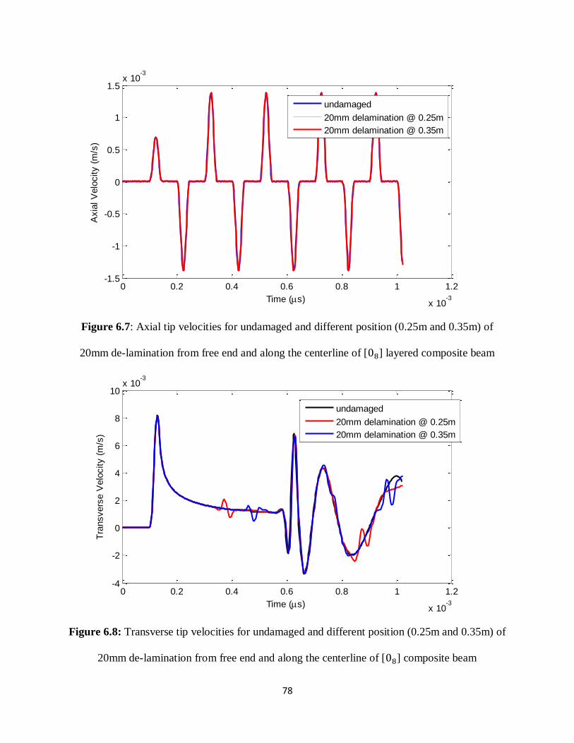
78

Figure 6.7: Axial tip velocities for undamaged and different position (0.25m and 0.35m) of

20mm de-lamination from free end and along the centerline of [ ] layered composite beam

Figure 6.8: Transverse tip velocities for undamaged and different position (0.25m and 0.35m) of

20mm de-lamination from free end and along the centerline of [ ] composite beam

0 0.2 0.4 0.6 0.8 1 1.2

x 10-3

-1.5

-1

-0.5

0

0.5

1

1.5x 10

-3

Time (s)

Axia

l V

elo

city (

m/s

)

undamaged

20mm delamination @ 0.25m

20mm delamination @ 0.35m

0 0.2 0.4 0.6 0.8 1 1.2

x 10-3

-4

-2

0

2

4

6

8

10x 10

-3

Time (s)

Tra

nsvers

e V

elo

city (

m/s

)

undamaged

20mm delamination @ 0.25m

20mm delamination @ 0.35m

79

The figure (6.7) and (6.8) shows the axial and transverse tip velocities of undamaged beam and

20mm de-lamination at different positions from the free end and along the centerline of the [ ]

layered composite beam. From figure (6.7), it is clearly observed that, the axial velocity of

undamaged beam and 20mm de-lamination at different positions from the free end and along the

centerline of the composite beam produce the same response. From figure (6.8), it can be

observed that the position of reflections due to the de-lamination changes by changing the de-

lamination position.

Figure 6.9: Axial tip velocities for undamaged and different depths above the centerline (h1=h,

h1=h/2 and h1=h/4) of 20mm de-lamination of [ ] layered composite beam

From figure (6.9) it can be observed that the response of undamaged and 20mm de-lamination at

=h i.e. at the centerline of the beam is same in the axial tip velocity. The response, for h1=h/2

and h1=h/4 gives undulations in the axial tip velocity. Where h1 is the depth of de-lamination

from the top surface of the beam.

0 0.2 0.4 0.6 0.8 1 1.2

x 10-3

-1.5

-1

-0.5

0

0.5

1

1.5x 10

-3

Time (s)

Axia

l V

elo

city (

m/s

)

undamaged

h1=h

h1=h/2

h1=h/4

80

Figure 6.10: Transverse tip velocities for undamaged and different depths above the centerline

(h1=h, h1=h/2 and h1=h/4) of 20mm de-lamination of [ ] layered composite beam

Figure 6.11: Axial tip velocities for different orientation ( , , , and ) of

20mm de-lamination along the centerline of composite beam

0 0.2 0.4 0.6 0.8 1 1.2

x 10-3

-4

-2

0

2

4

6

8

10x 10

-3

Time (s)

Tra

nsvers

e V

elo

city (

m/s

)

undamaged

h1=h

h1=h/2

h1=h/4

0 0.2 0.4 0.6 0.8 1 1.2

x 10-3

-5

-4

-3

-2

-1

0

1

2

3

4

5x 10

-3

Time (s)

Axia

l V

elo

city (

m/s

)

[0] 8layers

[30] 8layers

[45] 8layers

[60] 8layers

81

Figure (6.10) shows the transverse tip velocity of undamaged composite beam compared

with different depths above the centerline ( =h, =h/2 and =h/4) of 20mm de-lamination of

beam. Undulations can be observed from figure (6.10) by reducing the by which number of

undulations increases and the amplitude of these undulations initially decreases and later on

increases. In figure (6.11) and (6.12), comparing the axial and transverse tip velocities for

different ply orientation of , , , and layered composite beam with 20mm

de-lamination along the centerline. From these figures, it can be observed that the amplitude of

the undulations increases and shifting of these undulations occurs by increasing the ply

orientation.

Figure 6.12: Transverse tip velocities for different orientation ( , , , and ) of

20mm de-lamination along the centerline of composite beam

0 0.2 0.4 0.6 0.8 1 1.2

x 10-3

-0.01

-0.005

0

0.005

0.01

0.015

0.02

Time (s)

Tra

nsve

rse

Vel

ocity

(m

/s)

[0] 8layers

[30] 8layers

[45] 8layers

[60] 8layers

82

REFERENCES

83

REFERENCES

[1] Abdel Wahab, M.M. and De Roeck, G. Damage detection in bridges using modal

curvatures: Application to a real damage scenario. Journal of Sound and Vibration, 226:

217–235, 1999.

[2] Abdo, M.A.B. and Hori, M. A numerical study of structural damage detection using

changes in the rotation of mode shapes. Journal of Sound and Vibration, 251: 227–239,

2002.

[3] Amaratunga, K. and Williams, J. R. Wavelet –Galerkin solution of boundary value

problems. Archives of Computational Methods in Engineering, 4(3): 243-285, 1997.

[4] Amaravadi, V., Rao, V., Koval, L.R. and Derriso, M.M. Structural health monitoring

using wavelet transforms. Smart Structures and Integrated Systems. Proceedings of SPIE,

4327:258–269,2001.

[5] Bathe, K. J. Finite Element Procedures, Prentice Hall,1997.

[6] Batra, R.C and Ching H.K. Analysis of elasto dynamic deformation near a crack/notch

tip by the meshless local Petrov-Galerkin (MLPG) method. Computer Modeling in

Engineering and Sciences,3(6): 717-730, 2002

[7] Beskos, D. E. Boundary element method in dynamic analysis Part II (1986-1996).

Applied Mechanics Review, 50:149-197,1997.

[8] Beylkin, G. On the representation of operators in bases of compactly supported wavelets.

Society for Industrial and Applied Mathematics. Vol (6) 1716-1740,1992.

[9] Chakraborty, A., Mahapatra, D. R., Gopalkrishnan, S. Finite element analysis of free

vibration and wave propagation in asymmetric composite beams with structural

discontinuities, Composite Structures 55(1), 23-36, 2002.

84

[10] Chakrabborty, A., GopalaKrishnan, S. Poissions contraction effects in the deep

laminated composite beam, Mechanics of Advanced Materials and Structures 10(3) 205-

225, 2003.

[11] Chakrabborty, A., GopalaKrishnan, S., Reddy, J. A new beam finite element for

the analysis of functionally graded materials, International Journal of Mechanical

Sciences 45(3), 519-539, (2003).

[12] Chang, C.C. and Chen, L.W. Detection of the location and size of cracks in the

multiple cracked beam by spatial wavelet based approach. Mechanical Systems and

Signal Processing, 19:139–155, 2005.

[13] Chaudhari, T.D. and Maiti, S.K. A study of vibration of geometrically segmented

beams with and without crack. International Journal of Solids and Structures, 37:761–

779, 2000.

[14] Chinchalkar, S. Determination of crack location in beams using natural frequencies.

Journal of Sound and Vibration, 247:417–429,2001.

[15] Cao, M. and Qiao, P. Integrated wavelet transform and its application to vibration

mode shapes for the damage detection of beam-type structures. Smart Materials and

Structures, 17: 055014, 2008.

[16] Daubechies, I. Ten lectures on wavelets. CBMS-NSF Series in Applied Mathematics

(SIAM, Philadelphia), 1992.

[17] Douka, E., Loutridis, S. and Trochidis, A. Crack identification in beams using wavelet

analysis. International Journal of Solids and Structures, 40:3557–3569,2003.

[18] Douka, E., Loutridis, S. and Trochidis, A. Crack identification in plates using wavelet

analysis. Journal of Sound and Vibration, 270: 279–295, 2004.

85

[19] Doyle, J.F. Wave propagation in structures. Springer, New York,1999.

[20] GopalaKrishnan, S. A deep rod Finite Element for structural dynamics and wave

propagation problems, International Journal for Numerical Methods in Engineering 48

731-744, 2000.

[21] Gopalakrishnan, S., Chakraborty, A., and Roy Mohapatra, D. Spectral finite

element method: Wave propagation diagnostics and control in anisotropic and

inhomogeneous structures. Springer, 2007.

[22] Graff, K. F. Wave motions in elastic solids. Ohio State University Press,1975.

[23] Grassmann, A. and Morlet, J. Decomposition of hardy functions into square

integrable wavelets of constant shape. SIAM Journal of Mathematical Analysis,

15,723-736,1984.

[24] Hadjileontiadis, L.J., Douka, E. and Trochidis, A. Fractal dimension analysis for

crack identification in beam structures. Mechanical Systems and Signal Processing, 19:

659–674, 2005.

[25] Hadjileontiadis, L.J. and Douka, E. Crack detection in plates using fractal dimension.

Engineering Structures, 29: 1612–1625, 2007.

[26] Hao, H. and Xia, Y. Vibration-based damage detection of structures by genetic

algorithm. Journal of Computing in Civil Engineering, 16: 222–229, 2002.

[27] Hong, J.C., Kim, Y.Y., Lee, H.C. and Lee, Y.W. Damage detection using the

Lipschitz exponent estimated by the wavelet transform: applications to vibration modes

of a beam. International Journal of Solids and Structures, 39: 1803–1816, 2002.

86

[28] Hu, C.S. and Afzal, M.T. A statistical algorithm for comparing mode shapes of

vibration testing before and after damage in timbers. Journal of Wood Science, 52:

348–352, 2006.

[29] Jiang, L.J., Tang, J. and Wang, K.W. An enhanced frequency-shift-based damage

identification method using tunable piezoelectric transducer circuitry. Smart Materials

& Structures, 15: 799–808, 2006.

[30] Kasper, D.G., Swanson, D.C. and Reichard, K.M. Higher-frequency wavenumber

shift and frequency shift in a cracked, vibrating beam. Journal of Sound and Vibration,

312: 1–18, 2008.

[31] Kim, J.T. and Stubbs, N. Crack detection in beam-type structures using frequency

data. Journal of Sound and Vibration, 259: 145–160,2003.

[32] Kim, B.H., Park, T. and Voyiadjis, G.Z. Damage estimation on beam-like structures

using the multi-resolution analysis. International Journal of Solids and Structures, 43,

4238–4257.

[33] Lee, J.J., Lee, J.W., Yi, J.H., Yun, C.B. and Jung, H.Y. Neural networks-based

damage detection for bridges considering errors in baseline finite element models.

Journal of Sound and Vibration, 280: 555–578, 2005.

[34] Lele, S.P. and Maiti, S.K. Modelling of transverse vibration of short beams for crack

detection and measurement of crack extension. Journal of Sound and Vibration, 257:

559–583, 2002.

[35] Li, H.J., Li, H., He, C., Ji, J., Wang, H. and Hao, C. Crack damage detection in

beam-like structures using RBF neural networks with experimental validation.

87

International Journal of Innovative Computing Information and Control, 1: 625–634,

2005.

[36] Liang, R.Y., Choy, F.K. and Hu, J.L. Detection of cracks in beam structures using

measurements of natural frequencies. Journal of the Franklin Institute-Engineering and

Applied Mathematics, 328: 505–518, 1991.

[37] Mahapatra, D. R. & Gopalakrishnan, S. A spectral finite element model for analysis

of axial flexural shear coupled wave propagation in laminated composite beams.

Composites Structures 59, 67-88. (doi:10.1016/S0263-8223(02)00228-3), 2003.

[38] Mallat, S. G. Multiresolution approximation and wavelets. Preprint GRASP Lab.,

Department of Computer and Information Science. University of Pennsylvania, 1986 .

[39] Mansur, W. J. A time stepping technique to solve wave propagation problems using

the boundary element method. PhD Thesis, Southampton University,1983.

[40] Messina, A., Williams, E.J. and Contursi, T. Structural damage detection by a

sensitivity and statistical-based method. Journal of Sound and Vibration, 216: 791–808,

1998.

[41] Meyer, Y. Principle d’incertitude, bases hilbertiennes et algebres d’operateurs’. Volume

662. Seminaire Bourbaki, 1987.

[42] Mitra, M., GopalaKrishnan, S., Bhat, S. A new super convergent thin walled

composite beam element for analysis of box beam structures, International Journal of

Solids and Structures 41(5-6),1491-1518, 2004.

[43] Mitra, M. & Gopalakrishnan, S. 2005a Spectrally formulated wavelet finite element

for wave propagation and impact force identification in connected 1-D waveguides.

88

International Journal of Solids Structures 42, 4695-4721.

(doi:10.1016/j.ijsolstr.2005.02.007)

[44] Mitra, M. & Gopalakrishnan, S. Wavelet based spectral finite element modeling and

detection of de-lamination in composite beams. Proceedings of the Royal Society A

462, 1721-1740, 2006. (doi: 10.1098/rspa.2005.1653).

[45] Morassi, A. Crack-induced changes in eigenparameters of beam structures. Journal of

Engineering Mechanics-ASCE, 119: 1798–1803, 1993.

[46] Morassi, A. Identification of a crack in a rod based on changes in a pair of natural

frequencies. Journal of Sound and Vibration, 242: 577–596, 2001.

[47] Morassi, A. and Rollo, M. Identification of two cracks in a simply supported beam

from minimal frequency measurements. Journal of Vibration and Control, 7: 729–739,

2001.

[48] Morlet, J. Sampling theory and wave propagation. 233-261 in C. H. Chen (ed.), NATO

ASI Series, Issue in acoustic signal/ Image Processing and Recognition, Vol 1,

Springer, Berlin,1983.

[49] Morlet, J., Arens, G., Fourgeau, I., and Giard, D. Wave propagation and sampling

theory. Geophysics, 47: 203-236,1982.

[50] Murigendrappa, S.M., Maiti, S.K. and Srirangarajan, H.R. Experimental and

theoretical study on crack detection in pipes filled with fluid. Journal of Sound and

Vibration, 270: 1013–1032, 2004.

[51] Nag, A., Mahapatra, D. R., Gopalakrishnan, S. and Sankar, T. S. A spectral

finite element with embedded de-lamination for modeling of wave scattering in

composite beams. Composite Science and Technology, 63:2187-2200, 2003.

89

[52] Nandwana, B.P. and Maiti, S.K. Detection of the location and size of a crack in

stepped cantilever beams based on measurements of natural frequencies. Journal of

Sound and Vibration, 203: 435–446, 1997.

[53] Pandey, A.K., Biswas, M. and Samman, M.M. Damage detection from changes in

curvature mode shapes. Journal of Sound and Vibration, 145: 321–332, 1991.

[54] Pawar, P.M., Reddy, K.V. and Ganguli, R. Damage detection in beams using spatial

Fourier analysis and neural networks. Journal of Intelligent Material Systems and

Structures, 18: 347–359, 2007.

[55] Poudel, U.P., Fu, G.K. and Ye, H. Wavelet transformation of mode shape difference

function for structural damage location identification. Earthquake Engineering &

Structural Dynamics, 36: 1089–1107, 2007.

[56] Qian, S. and Weiss, J. Wavelets and the numerical solution of boundary value

problems. Applied Mathematics Letter, 6(1): 47-52,1993.

[57] Qian, S. and Weiss, J. Wavelets and the numerical solution of partial differential

equations. Journal of Computational Physics, 106(1): 155-175,1993.

[58] Qiao, P. and Cao, M. Waveform fractal dimension for mode shape-based damage

identification of beam-type structures. International Journal of Solids and Structures,

45: 5946–5961, 2008.

[59] Rahai, A., Bakhtiari-Nejad, F. and Esfandiari, A. Damage assessment of structure

using incomplete measured mode shapes. Structural Control & Health Monitoring, 14:

808–829, 2007.

[60] Ren, W.X. and De Roeck, G. Structural damage identification using modal data. I:

Simulation verification. Journal of Structural Engineering-ASCE, 128: 87–95, 2002.

90

[61] Ren, W.X. and De Roeck, G. Structural damage identification using modal data. II:

Test verification. Journal of Structural Engineering-ASCE, 128: 96–104, 2002.

[62] Rucka, M. and Wilde, K. Application of continuous wavelet transform in vibration

based damage detection method for beams and plates. Journal of Sound and Vibration,

297: 536–550, 2006.

[63] Ruotolo, R. and Surace, C. Damage assessment of multiple cracked beams: Numerical

results and experimental validation. Journal of Sound and Vibration, 206: 567–588,

1997.

[64] Salawu, O.S. Detection of structural damage through changes in frequency: A review.

Engineering Structures, 19: 718–723, 1997.

[65] Shi, Z.Y., Law, S.S. and Zhang, L.M. Damage localization by directly using

incomplete mode shapes. Journal of Engineering Mechanics-ASCE, 126: 656–660,

2000.

[66] Shorr, B. F. The wave finite element method. Springer, Berlin,2004.

[67] Stormberg, J. O. A modified Frankiln system and higher order spline system on as

unconditional bases for hardy spaces. Pages 475-493. Conf. in Honour of A. Zygmund,

Vol II, Wadsworth Mathematics Series, 1982.

[68] Swamidas, A.S.J. and Chen, Y. Monitoring crack-growth through change of modal

parameters. Journal of Sound and Vibration, 186: 325–343, 1995.

[69] Wang, J. and Qiao, P.Z. Improved damage detection for beam-type structures using a

uniform load surface. Structural Health Monitoring-an International Journal, 6: 99–

110, 2007.

[70] Wen Shen. Lecture Notes for Laplace Transform. April 2009.

91

[71] Williams, J. R. and K. Amaratunga, K. A discrete wavelet transform with out edge

effects using wavelet extrapolation. Journal of Fourier Analysis and Applications, 3(4):

435-449,1997.

[72] Zhong, S.C. and Oyadiji, S.O. Crack detection in simply supported beams without

baseline modal parameters by stationary wavelet transform. Mechanical Systems and

Signal Processing, 21: 1853–1884, 2007.

[73] Zhong, S., Yadiji, S.O. and Ding, K. Response-only method for damage detection of

beam-like structures using high accuracy frequencies with auxiliary mass spatial

probing. Journal of Sound and Vibration, 311: 1075–1099, 2008.