DEHRADUN INSTITUTE OF TECHNOLOGY LABORATORY …eedofdit.weebly.com/uploads/7/3/2/6/7326910/lab_manual_control_lab_to... · controller using simulated systems. DEHRADUN INSTITUTE OF

DEHRADUN INSTITUTE OF TECHNOLOGY LABORATORY MANUAL

PRACTICAL INSTRUCTION SHEET

EXPERIMENT TITLE: To study the performance characteristics of an analog PID

controller using simulated systems.

EXPERIMENT NO. : ISSUE NO. : ISSUE DATE :

REV. NO. REV. DATE : 01/08/2016 PAGE /

DEPTT. : Electrical

Engineering LABORATORY : Control System EA5220 SEMESTER : V

PREPEARD BY :- Mr. Husain Ahmed

APPROVED BY :- Dr. Gagan Singh

Visit us at www.eedofdit.weebly.com

Objective:

To study the performance characteristics of an analog PID controller using simulated

systems.

Apparatus Used:

Name of the apparatus Range/Rating Quantity

1. PID System 1

Proportional Gain : 0 to 20

Integral time constant : 5 – 100 msec

Derivative time constant : 0- 20 msec

Theory:

The performance of a physical system is not always good enough for a given

application. In such a situation the characteristics of the system needs to be modified. This is

referred to as “compensation design”. Standard procedure available for compensation include

time and freq domain designs of a variety of compensation networks .such design methods have

been successfully used in many practical dynamic control systems.







DEPTT. : Electrical





The performance of the system is evaluated in terms of a set of performance specifications e.g.

rise time, peak time, settling time, peak percent overshoot and steady and steady state error in the

time domain and gain margin phase margin, closed loop bandwidth etc. in the frequency domain.

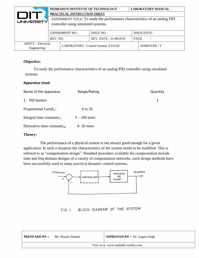
Another approach towards improving the performance of systems has been through

elementary control actions called control terms- inserted in the forward path of an existing

control system. The block diagram of fig 1 shows the location of such a controller in a unity

feedback system. The controller work comprises two or three of the following control terms:

a) Proportional, P

b) Integral, I

c) Derivative, D

The resulting control system may turn out to be a PI, PD or PID controller.

The two and three term controllers indicated above have been used more commonly by process

industries e.g. Petroleum, chemical, powder, food etc. for the control of temperature, pressure,

flow and similar variable. A common features of these system is their sluggish response which

calls for accurate and slow integration and sensitive differentiation. Although near ideal

electronic differentiator and integrator circuits are difficult to achieve except with high

temperature operational amplifiers and good quality component PI and PD controller valves

have existed in the pneumatic and hydraulic environment for a long time.

In the present unit attempt has been made to expose the student to the study and design of

PID controller using simulated systems. The speed of response has been deliberately scaled up

to have a fast and easy viewing on CRO.

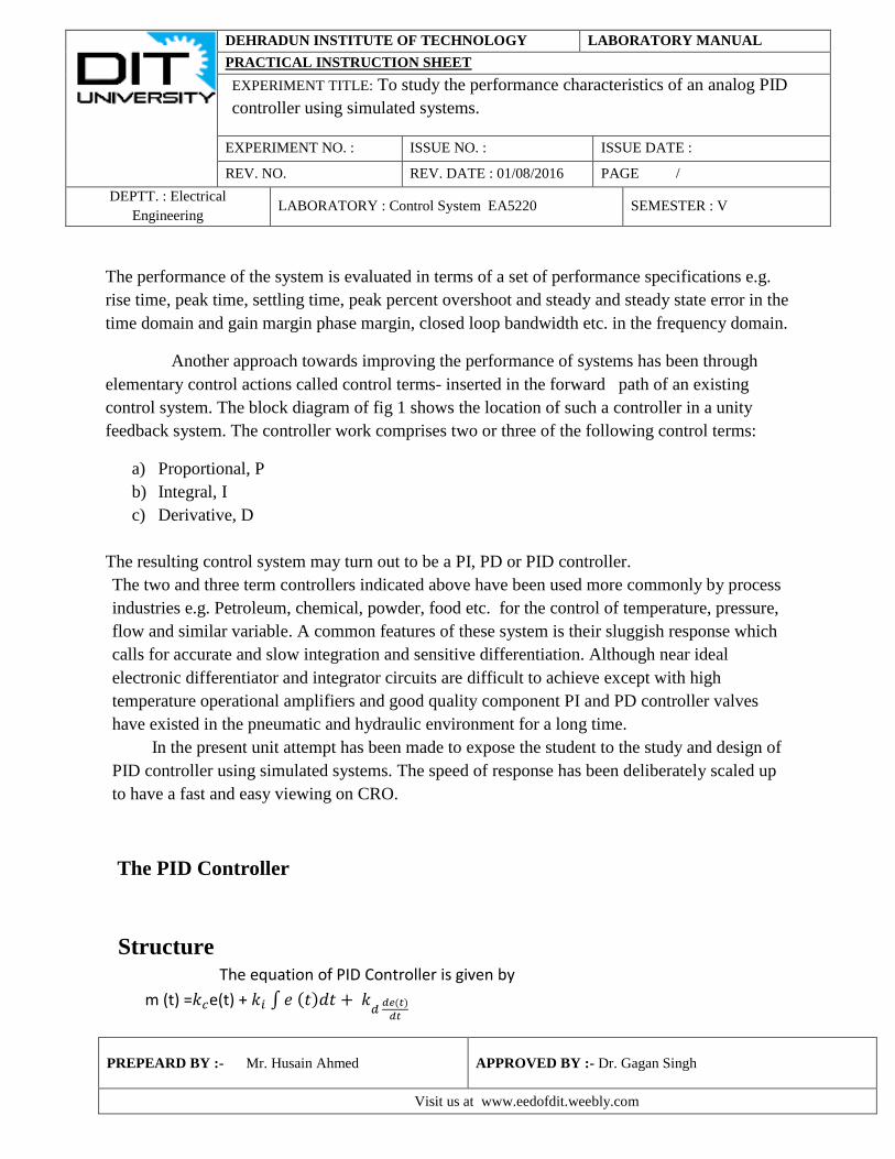
The PID Controller

Structure The equation of PID Controller is given by

m (t) = e(t) +







DEPTT. : Electrical





Where e (t) = error signal

m (t) = PID o/p or plant i/p

=proportional gain

= integral gain

=derivative gain

In the Laplace domain, the above eq is written as







DEPTT. : Electrical





M(s) = E(s) +

E (s) + s E(s)

Which may be represented as the block diagram of fig.3

An alternative representation of the above which is more commonly used I process

control literature is as under:

M(s) = (1 +

+ s) E(s)

Where

=

= Integral time constant

=

=derivative time constant

It is easy to develop the structure of PD, and PI controllers from above , substituting =0 and

=0 respectively.

A special terminology used in process control literature is given below to facilitate better

understanding.

Proportional Band =

x 100 %

Reset rate =

=

per minute

Derivative Time =

In the present unit, the three gains are adjustable in the following range with the help of

calibrated 10- turn potentiometers.

: 0 to 20

: 0 to 1000

: 0 to 0.01







DEPTT. : Electrical





Experimental determination of these values are discussed in sec .4

CHARACTERISTICS

From eq (2) the transfer function of the PID controller may be written as (s) =

=

=

(s + ) ( s + )

Where and are the two zeroes of the PID controller transfer function.

The above transfer has a pole at the origin and two real zero for







DEPTT. : Electrical





Notice that a properly designed PID controller should not, in general, have pair of complex

conjugate zeroes which may result in reduced damping. Bode diagram of the PID controller is

shown in fig. 3.

It may be seen that the controller gain increase without limits as the frequency is

decreased. This is due to the integral term, and it results in a reduction of steady state error.

However, the negative phase angle introduce by the controller at low frequencies has a

destabilizing effect as well. The corner frequency should therefore be so located that large

negative phase angle occurs at sufficiently low frequencies only, where the plant already has a

good stability margin.

Again, the bode diagram of the controller an increased gain at high frequencies

accompanied by a positive phase angle. The positive phase angle has a stabilizing effect while

the large gain at high frequencies makes the system more responsive to fast or sudden changes.

The overall system then becomes relatively more stable, as it capable of taking ‘anticipatory’

action in the presence of signal having fast variation.

Design

The PID controller can be designed both in frequency domain and in the s-plane,

through the classical or trial and error design procedure. The method needs the pole zero location

or frequency phase response of the plant, for its implementation. A large number of process

control systems are however characterized by,

Incomplete or inaccurate plant questions.

Extremely slow response.

Presence of time delays.

High order transfer function

Limited possibility of experimentation for identification of the plant, and

Need for fine trimming the compensator at site

In such a situation alternative simpler technique of setting the controller parameter

( , ), or tuning are of great practical value. Presented below are three technique of

tuning a PID controller aimed at obtaining a satisfactory step response of the overall

system. Experimental work based on this method.







DEPTT. : Electrical





(a)Trial and error tuning

This is a simple and systematic method for on the line tuning of a PID controller. The

method assumes that the three parameters are available for adjustment. Following are

steps for its implementation:

1. Disconnect or reduce derivative and integral block signals by setting to

zero.

. 2. Starting from a low value increase gradually oscillation sets in .this condition is

tested by small disturbances generated by varying the reference signal a little. The value

by proportional gain so obtained is called ultimate gain .

3. Set to ½ of the value obtained in step 2.

4. Increase gradually until sustained oscillations start again. Set to 1/3 of this value.

5. Increase gradually until sustained oscillations start again. Set to 1/3 of this value.

The above method, although very simple in operation, has the following

limitations:

I. A number of systems which are or may be approximated, first or second order

transfer functions without time delay do not oscillate. Step 3 is then not possible

and the method fails.

II. Open loop unstable systems cannot be handled by this method.

III. Tuning of very slow systems by this method is extremely time consuming.

IV. Sustained oscillation may not be acceptable or may be risky in some physical

process such as a large chemical process.

(b) Continuous Cycling Method







DEPTT. : Electrical





In this method given by Ziegler and Nichols the first step is to determine

experimentally the value of ultimate gain, as suggested in the previous method. The

time period of the resulting sustained oscillations is referred to as ultimate period .

Based on the values of and the controller setting are obtained from Table 1 which

as essentially empirical in nature.

Controller Type

P 0.5 - -

PI 0.45 0.833 -

PID 0.6 0.5 0.125

The values of and may be calculated from eq.3 for implementation on the

present system.

Some variation in the coefficient settings have also been suggested by various

workers. In any case the above values should be taken as the initial settings and should

invariably be followed by the fine tuning via trial and error.

Most of the limitations of the first method are still present in this method.

However the continuous cycling method is less time consuming.

Process Reaction curve Method







DEPTT. : Electrical





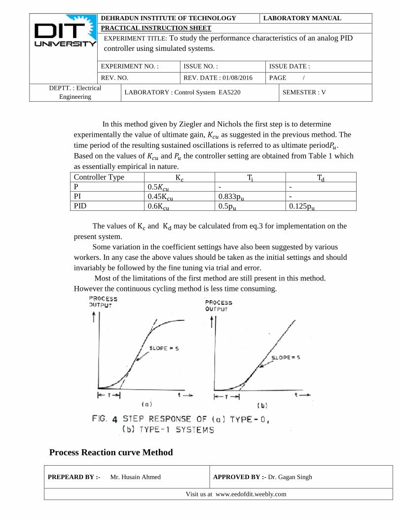
This is a second on line method purposed by Ziegler and Nichols and is very attractive

because it is based on a simple experiment. The plant is modelled as a first order function with

time delay. The open loop step response of the plant, called reaction curve of the process. Is

experimentally obtained. Typical step response for type-0 and higher type number system are

shown in fig 4(a) and 4(b) respectively. The step responses are characterized by two parameters,

(I) Slope S of the tangent drawn at the point of inflection, and

(II)Time T at which the tangent intersects the X axis.

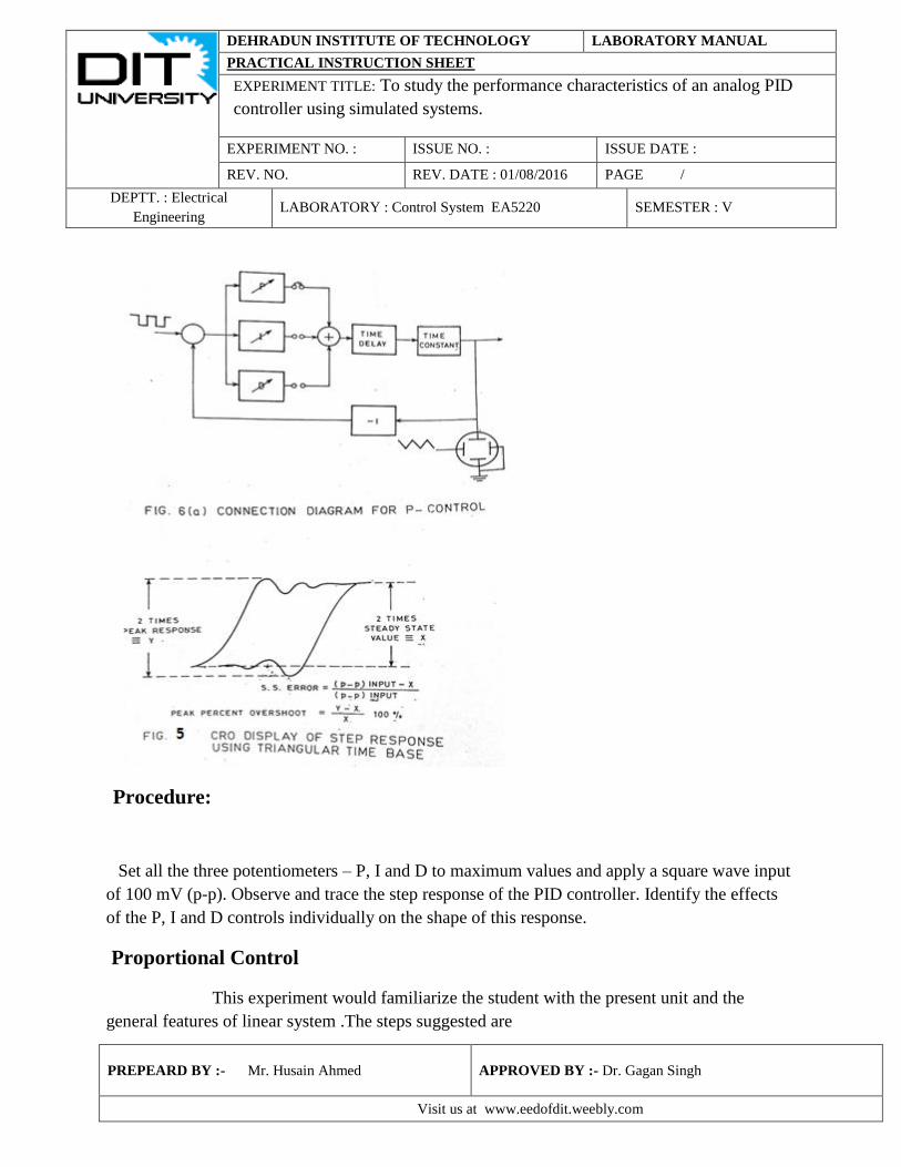
The values of S and T are obtained graphically as shown in fig 5. In the input step changes was

M the PID parameters are given by the Table below.

Controller Type

P

- -

PI

3.33T -

PID

2T 0.5T

Once again, the above values are empirical in nature and therefore fine tuning of the parameters

may be needed in specific cases. The values of and may be calculated from eq. 2 for

implementation on the present unit.

Although the process reaction curve method based on a single experimentation is fast and

simple, it does have some limitations as given below:

i. The step response obtains in the open loop may not be satisfactory in case the

system is highly nonlinear or open loop unstable.

ii. Accuracy is limited due to the graphical procedure involved.

In conclusion it may be said that any method used to calculate the parameters must be followed

by a fine tuning on the operational process.







DEPTT. : Electrical





EXPERIMENTS

A very wide range of experimentation is possible with the unit, however the ones

suggested below are aimed at bringing out the feature of PID controller in one or two laboratory

classes of usual duration. It may be mentioned that a conventional CRO display has been

obtained by a proper design of the system. Tuning of PID controller is therefore very fast and

avoids expensive accessories like an X-Y/t recorder.

Experimentation in the following material has been suggested with a system having a time

delay block .Such a representation is closer to many real life systems which have pure time

delay. However this takes the system closer to instability which can then accept only small

values of , etc. As a result the settings of P,I and D controls may be difficult to make for a

beginner . In that case it is suggested that the beginner may experiment with a system with one /

two time constant blocks without time delay block.

Before starting the experiments, it will be helpful to understand the calibrated dials of P, I and D

control knobs. In section 4.1, the student finds the maximum value of , and or in other

words the full scale values of these parameters. The potentiometers used are 10 turn types and

each turn is divided into 10 parts by the dial scale. Each part is further divided into 5 divisions so

that the total dial range of 0 to 1 has a least count of 0.002. A full revolution of a knob

corresponds to a change of 0.1 in dial reading. To obtain a parameter value , multiply the dial

setting by the corresponding full scale (FSV) for P control is 20 then a dial setting of 0.032 will

correspond to a =0.032 x 20 = 0.64.

CONTROLLER RESPONSE

The time domain response of the PID controller is of great value for a good understanding of its

performance. This also enables the readers to calibrate the three potentiometers, it felt necessary.

The steps suggested are:

1. Apply a square wave signal of 100 mV p-p at the i/p of the error detector. Connect P, I

and D outputs to the summer and display controller o/p to the CRO.

2. With P potentiometer set to maximum and I and D potentiometers set to 0 , obtain

maximum value of as :







DEPTT. : Electrical





3. With I potentiometer set to maximum and P and D potentiometers set to 0,a ramp will be

set on CRO. Maximum value of is given by :

Max =

Of the input

4. Set D potentiometer to maximum P and I potentiometers to 0. A series of sharp pulses

will be seen on the CRO. This is obviously not suitable for calibrating the D

potentiometer. Instead applying a triangular wave at the input of the error detector a

square wave is seen on the CRO.

Max =







DEPTT. : Electrical





Procedure:

Set all the three potentiometers – P, I and D to maximum values and apply a square wave input

of 100 mV (p-p). Observe and trace the step response of the PID controller. Identify the effects

of the P, I and D controls individually on the shape of this response.

Proportional Control

This experiment would familiarize the student with the present unit and the

general features of linear system .The steps suggested are







DEPTT. : Electrical





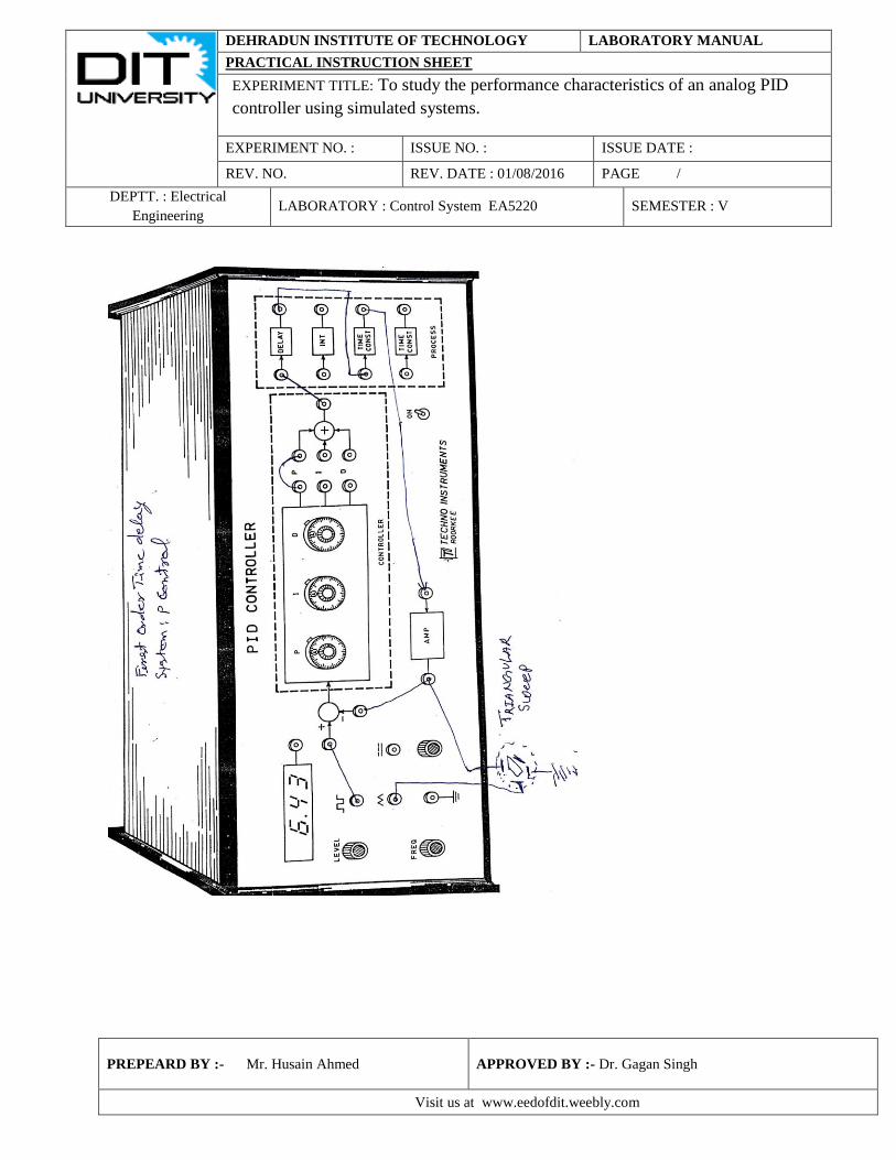
Make connections as shown in Fig.6 (a) with process made up of time delay and time

constant blocks. Notice that the CRO operation in X-Y mode ensure stable display even

at low frequencies.

Set input amplitude to 1V (p-p), and frequency to a low value.

For various values of =0.2, 0.4… measure from the screen the values of peak

overshoot and steady state error and tabulate (Refer to Fig.6 (b) for graphical

calculation).

Alternatively, a simultaneous display of square wave input and system response

using a dual trace oscilloscope may be used to get a very clear idea of the

transient and steady state performances. Some flickering may however be

observed in this case due to the low frequencies involved.

Observe that the second order type-0 system has non-zero steady state error for step input which

decreases with increasing while the peak overshoots increases.

The above experiment may be performed for a variety of system with or without

time delay. Note that loop phase must be kept as 180*, if necessary by using the uncommitted

amplifier of gain = -1, so that the feedback is negative.

Proportional – Integral Control

The integral term results in increasing the system type number by unity and thus

cause improvement in steady state performance. To verify the above with step input one starts

with a type-0 system having a non-zero error. Introducing PI control with a properly selected

value of Ti should reduce the error to zero. The steps suggested are as follows:

Make connections for a 1st order type-0 system with time delay (Fig. 6(a) with

proportional and integral blocks connected).

Set input amplitude to 1V (p-p), frequency to a low value and K to zero.

For =0.6(say), observe and record the peak overshoot and steady state error.

With the Kc as above, increase Ki in small steps and record peak overshoot and steady

state error.

Observe that for a given value of increasing of integral gain improves the steady state

performance. Excessive increase of , however results in an inferior transient response







DEPTT. : Electrical





For a detailed study of proportional control, our experimental control, our experimental set-up

“Linear System Simulator” is recommended.

Proportional-Integral-Derivative Control

This experiment will demonstrate the improvement in transient performance by the

introduction of derivative control. The following steps suggested:

Make connections as shown in figure 6(a) with proper integral and derivatives blocks

connected.

Set the input amplitude to 1V (p-p), frequency a low value, =0.6, =54.85 and

=0.

The system shows a fairly large overshoot. Record the peak overshoot and steady state

error.

Repeat the above step for a few non-zero values of

Observe the improvement in transient performance with increasing

values of , while the steady state error remains unchanged.

For =0.6, adjust and by trial and error to obtained the best overall response.

Record the values of , and . Repeat for =0.4, 0.2 etc.

PID Design by Process Reaction Curve Method

In this experiment the PID parameters are designed by the method of Ziegler and Nichols

outlined in sec. 3.23(c). The Unit step response of the open loop system is obtained first.

Subsequent steps are:

Compute S and T from The CRO screen as indicated in fig.(a).

Calculate the parameters of PID controller from Table 2 which are reproduced below:

=







DEPTT. : Electrical





= 2T, or =

=0.5T, or =

Set the PID parameters as calculated above and the observe the response. Comment.

Attempt fine tuning parameters to get a better response.

All the above mentioned experiments may be carried out on a variety of plants of

different orders and type numbers depending on the time allotted in the curriculum.

RESULTS:

Calibration

The calibration results here corresponded to the measurements suggested in

section 4.1

a) P Control Input: Square wave of amplitude 0.1 V (p-p)

Output: Square wave of amplitude 2.0 V (p-p)

(max.): 2.0/0.1 = 20

b) I Control Input: Square wave of amplitude 0.1 V (p-p)

Time period: 70 msec

Frequency: 1000/70 = 14.286 Hz

Output: Triangular wave of amplitude 1.6 V (p-p)

(Max.) = 4*14.286*1.6/0.1 = 914.2/sec

c) D Control Input: Triangular wave of amplitude 0.84 V (p-p)

Time period: 70 msec

Frequency: 1000/70 = 14.286 Hz

Output: Square wave of amplitude 0.5 V (p-p)

(max.) = 05/4*14.286*0.84 = 0.0104 sec

PI Control







DEPTT. : Electrical





Input: 1V (p-p) Square wave of low frequency

= 0.6

System = type 0 with the time delay fig 6(a)

Scale Reading (per

sec.)

X=2*Steady

state value

Y=2*peak

response

Steady state

error

% overshoot

0.00 0.00 0.50 0.56 0.50 12.00

0.02 18.28 0.60 0.64 0.40 6.67

0.04 36.57 0.72 0.76 0.28 5.55

0.06 54.85 0.84 0.96 0.16 14.28

0.08 73.14 0.92 1.16 0.08 26.08

This system, due to the presence of time delay block, has a greater tendency to become

unstable. Readings are therefore restricted to small values of Kc ad Ki. System without

time delay will operate satisfactory over wide range of gain values and are recommended in

the initial stages of experimentation.

PID Control

Input: 1V (p-p) Square wave of low frequency

= 0.6

= 0.606*914.2 = 54.85/sec.

System = type – 0 with time delay

Scale

Reading (sec.) X=2*Steady

state value

Y=2*peak

response

Steady state

error

% overshoot

0.00 0 0.8 0.94 0.2 17.5

0.05 .52*

0.8 0.88 0.2 10.0

.10 1.04*

0.8 0.84 0.2 5.0

0.15 1.56*

0.8 Overdamped

(no overshoot)

0.2 -







DEPTT. : Electrical





The trial and error value for best performance (of the system shown in fig. 6(a) in

the prototype for Kc = 0.4 were found as:

= 0.065*914.2 = 59.423 per sec.

= 0.08*0.0104 = 0.832* sec.

Precaution:

1. Do not increase the range of P, I and D randomly.

2. Connect the terminals properly.

.







DEPTT. : Electrical





Documents

DEHRADUN INSTITUTE OF TECHNOLOGY LABORATORY …eedofdit.weebly.com/uploads/7/3/2/6/7326910/lab_manual_control_lab_to... · controller using simulated systems. DEHRADUN INSTITUTE OF