III

DEGREE PROJECT Metals working engineering

Programme Extent

Materials Design and Engineering, 300 ECTS 30 ECTS Name of student Year-Month-Day

Nina Hedlund 2014-09-06 Supervisor Examin

er

Mikael Olsson Anders Eliasson Company Supervisor at the Company

Atlas Copco Rock Drills AB Jonas Svensson Title

Experimental simulation of cavitation erosion

Keywords Cavitation, Cavitation Erosion, Cavitating Liquid Jet, Bronze alloys

ABSTRACT

This thesis includes a study of cavitation erosion and a Jet Cavitation Erosion Rig which is a test equipment used to generate cavitation erosion under well defined conditions.

The experimental work was to rank the relative cavitation erosion resistance using the Jet Cavitation Erosion Rig for three copper alloys; aluminum-, tin-, and leaded tin bronze. The work was performed in two steps: first the optimized parameters to create as much material loss as possible in a short time were to be find and then a number of tests series were carried out with these parameters to rank the cavitation erosion resistance of the bronzes. The ranking of the bronzes were made based on their incubation period and the volume loss rate in the initial stage. The tests in the cavitation rig were limited to one kind of fluid, hydraulic oil.

The ranking, i.e. the cavitation erosion resistance, of the bronzes obtained using the Jet Cavitation Erosion Rig was found to be the same as the ranking displayed in rock drilling applications in the field. Thus, aluminum bronze was found to have the best resistance followed by tin bronze and leaded tin bronze. Consequently, it can be concluded that the Jet Cavitation Erosion Rig can be used to evaluate the relative cavitation erosion resistance of materials used in this kind of applications.

IV

V

EXAMENSARBETE, D-nivå Bearbetningsteknik

Program Omfattning

Materialdesign, 300 hp 30 hp Namn Datum

Nina Hedlund 2014-09-06 Handledare Examinator

Mikael Olsson Anders Eliasson Företag Handledare vid företaget

Atlas Copco Rock Drills AB Jonas Svensson Titel

Experimental simulation of cavitation erosion

Nyckelord

Kavitation, Kavitationserosion, Cavitating Liquid Jet, Bronslegeringar

SAMMANFATTNING (SWEDISH)

Detta examensarbete innefattar en studie om kavitationserosion och även Jet Cavitation Erosion Rig som är en testutrustning som används för att generera kavitationserosion under väldefinierade förhållanden.

Det experimentella arbetet gick ut på att rangordna det relativa motståndet mot kavitationserosion vid användning av just Jet Cavitation Erosion Rig hos tre olika kopparbaslegeringar; aluminium- , tenn- och blybrons. Detta arbete utfördes i två steg, där det första var att optimera parametrar för att skapa en så stor materialavverkning som möjligt på kort tid och därefter kördes ett antal testserier med utvalda parametrar för att ranka bronserna. Rankingen av bronserna gjordes utifrån deras inkubationstid och graden av volymavverkning i inledande skede. Testerna i kavitationsriggen avgränsades även till en typ utav vätska, hydraulolja.

Rankingen av bronserna utifrån deras motstånd mot kavitationserosion i kavitationsriggen visade sig bli densamma som den som redan var känd utifrån användande i bergborrmaskiner. Alltså, aluminiumbronset visade sig ha bäst motstånd följt av tennbrons och blybrons. Därmed bestämdes att kavitationsriggen är lämplig att använda för att jämföra relativ resistensförmågan mot kavitationserosion för denna typ av konstruktionsmaterial.

VI

VII

FOREWORD

I’m very grateful I had the opportunity to perform this thesis at Atlas Copco Rock Drills AB. The mission was to determine if the Jet Cavitation Erosion Rig could be useful as a test equipment to rank cavitation erosion resistance at Atlas Copco Rock Drills AB. It was also the final part of the M.Sc. Material Science and Engineering education at Dalarna University in Borlänge, Sweden.

I’m also very grateful to my supervisor from Atlas Copco Rock Drills AB, M.Sc Jonas Svensson and Prof. in Materials Science Mikael Olsson from Dalarna University and want to give my gratitude to them for the help and guiding they provided during the work. I would also like to thank Manager Ph.D, Sima Valizadeh, global function manager and M.Sc Andreas Jansson at Materials Competence for the exceptional guidance and help during my time at Atlas Copco Rock Drills AB. Finally I also want to give my thanks and gratitude to Tor Persson, Manager at Rock Drills Lab for the help with the experimental work, and additional staff within Atlas Copco Rock Drills AB who gave support and help with my thesis.

Nina Hedlund Örebro, June 2014

VIII

IX

TABLE OF CONTENTS

1. INTRODUCTION ................................................................................ 1

1.1 Background ................................................................................... 1 1.2 Aim ................................................................................................ 1 1.3 Limitations .................................................................................... 2

2. THEORY .............................................................................................. 3 2.1 Cavitation erosion ......................................................................... 3 2.2 Cavitation testing .......................................................................... 5

3. EXPERIMENTAL DETAILS ................................................................9 3.1 Experimental set- up and equipment design ................................9 3.2 Specification of selected materials .............................................. 10 3.3 Sample preparation and geometry ............................................. 13 3.4 Experimental procedures ............................................................ 14 3.5 Characterization techniques ....................................................... 14

4. EVALUATION OF TEST PARAMETERS .......................................... 16 4.1 Experimental execution .............................................................. 17 4.2 Results and discussions .............................................................. 18 4.3 Conclusion ................................................................................... 27

5. RELATIVE CAVITATION RESISTANCE ......................................... 29 5.1 Experimental execution ............................................................. 29 5.2 Results and discussions ............................................................. 29 5.3 Conclusion .................................................................................. 40

6. FUTURE WORK ................................................................................ 41 7. REFERENCES .................................................................................. 42 APPENDIX I Equations ........................................................................... 45 APPENDIX II Figures from tests in chapter 4.2 ..................................... 46 APPENDIX III Figures from tests in chapter 5.2 ..................................... 50

1

1. INTRODUCTION

1.1 Background

Atlas Copco Rock Drills AB is situated at a number of places around the world where Rocktec is a division within Atlas Copco’s Mining and Rock excavation business area. The division designs, develops and manufactures rock drills, rotation units and automation solutions in the form of rig control systems. Rock excavation equipment operates during very severe conditions, above as well as under the ground, all around the globe. They must operate in an equally excellent way in extreme cold as in tropical heat, soaked with highly corrosive mine water, and covered with stone dust. In addition, the equipment is exposed to complex load conditions, impact loads, etc. during operation, which naturally put high demands on used materials.

Cavitation erosion is one failure mechanisms of hydraulic components in hydraulic rock drills as well as other systems involving rapid pressure fluctuations in fluids. Cavitation erosion is often observed as surface pits caused by local surface plastic deformation and localized wear. The damage according to cavitation erosion occurs when the cavities in the hydraulic oil collapses and affects the surrounding material. Cavities arise in the fluid when the pressure decreases to a value below the vapour pressure of the fluid (e.g. hydraulic oil) [1].

Due to differences in pressure during drilling the components of the equipment may be exposed to cavitation erosion which causes problems associated with surface deformation and wear eventually causing severe failure. The shape changes in material surfaces leads to significant changes in wear resistance, reduced efficiency and most important limited the component life in hydraulic rock drills.

The exposed components in hydraulic rock drills at Atlas Copco Rock Drills AB are typically made of bronze alloys; aluminum-, tin- and leaded tin bronze. Based on experience from the field it is known that the aluminum bronze shows the highest cavitation erosion resistance, followed by tin bronze and leaded tin bronze.

As described in literature several test equipments for testing cavitation erosion can be used, e.g. the Vibratory apparatus (ASTM G32), the Rotating disc and Liquid jet (ASTM G134) [2,3]. The systems are primarily used to test cavitation erosion in water. However, there are very limited or none information exists regarding the affectivity of these testing equipments when using hydraulic oil as a fluid to predict the cavitation resistance for different materials.

In the presented study the erosion rates for three kinds of bronze alloys were clarified according to the ASTM G134 standard [2].

1.2 Aim

The goal of this investigation was to verify and optimize the cavitation rig, Jet Cavitation Erosion Rig (based on ASTM G134), when using hydraulic oil as fluid.

When using a Jet Cavitation Erosion Rig the degree of cavitation damage can varies by different parameters, such as inlet pressure and stand- off distance. Therefore at first approach it was intended to obtain the maximum cavitation damage in a short

2

time. Second, investigate the cavitation erosion resistance of different materials while the test times kept down.

Finally, in order to find out and evaluate the most compatible cavitation resistance alloy when using hydraulic oil in hydraulic rock drills, the experiments was continued based on the optimized parameters as mentioned above.

1.3 Limitations

The cavitation rig could only be run with one type of hydraulic oil. Thus, differences between different fluids to study the erosion on material surfaces could not been investigated.

It was not possible during the tests to control the outlet pressure. The temperature for the hydraulic oil was approximately fixed between 40-60ºC.

The first test, Test 1.1, was run without any weight loss measurements and consequently no material loss data from this test can be reported.

Except from some limited microscopy, the thesis work does not involve no closer examination of the cavitation damage mechanisms. The focus was instead to find the optimized parameters and the relative resistance to cavitation erosion.

3

2. THEORY

2.1 Cavitation erosion

Cavitation erosion is a type of erosion which occurs on solid surfaces due to cavitation in flowing and vibrating fluids. It may cause unwanted effects such as surface deformation and material loss on an existing design [4]. Different materials exhibit different degrees of resistance to cavitation erosion and the prediction of all effective parameters to study the cavitation impact on materials requires great knowledge of both the selected material and the tribosystem. The parameters that are affecting the cavitation erosion failure mechanisms are discussed below.

Pressure When the pressure decreases in fluid cavities could be formed. Those cavities in a fluid will grow when the fluid can’t manage to stay together due to fluid starvation [5]. But when the pressure again increases and causing compressive stresses in the fluid the cavities will stop growing, followed by collapses [4]. The cavity will collapse in such a way that the upper wall moves towards the bottom wall of the cavity until it makes contact [6]. Here the cavity can turn into two new (but smaller) cavities by the stream of fluid and create the so called micro-jet phenomenon. If the micro-jet hit a material surface it can produce microscopically plastic deformation in the shape of a pit or material loss [7]. The phenomenon is schematically shown in Figure 1.

Figure 1. A schematic sketch of the micro-jet phenomenon [7].

These pits arises one at a time on the material surfaces, but as the number of pits increases they tend to congregate and form clusters of pits. This is explained in that already deformed surfaces, acts as “cavitation generators” where the cavities accumulate at the existing pits and even implodes in that area. This phenomenon is probably due to that the deformed areas may have reduced resistance to further damage and that the irregularities on the surface causing the cavities to gathered around them [8].

Surface tension The surface tension has a stabilizing effect on dynamic processes such as cavity growth and collapses. This effect appears to be strong when the size of the cavity is small [9]. The formation of a cavity has to overcome the resistance that the surface tension in the surrounding fluid provides [10]. Since the surface tension of water is higher (approx. 70mN/m) than in oil (approx. 30mN/m) it is harder to overcome the resistance to create cavities in water. But the cavitation damage can be more severe using water as the fluid, since the cavities grow bigger and thereby generate higher erosive power when they implode [11,12,13].

4

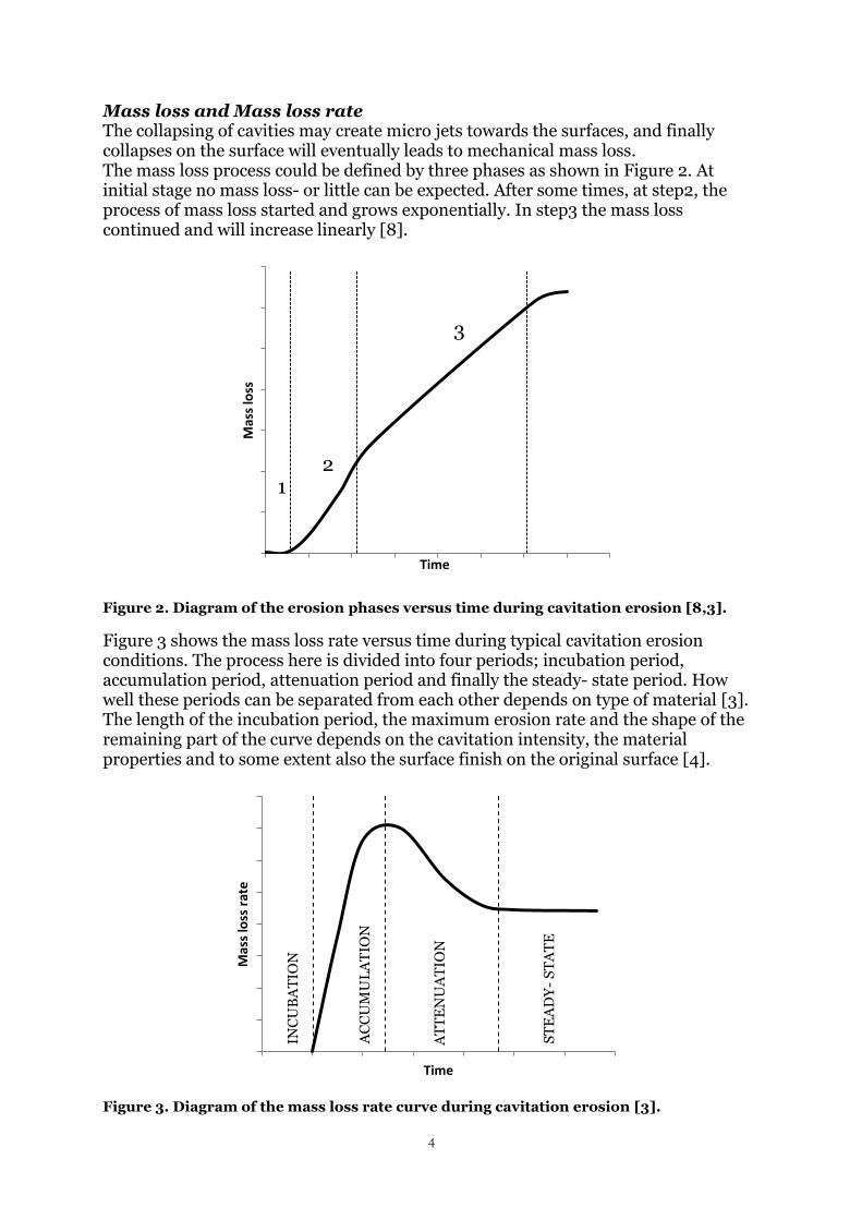
Mass loss and Mass loss rate The collapsing of cavities may create micro jets towards the surfaces, and finally collapses on the surface will eventually leads to mechanical mass loss. The mass loss process could be defined by three phases as shown in Figure 2. At initial stage no mass loss- or little can be expected. After some times, at step2, the process of mass loss started and grows exponentially. In step3 the mass loss continued and will increase linearly [8].

Figure 2. Diagram of the erosion phases versus time during cavitation erosion [8,3].

Figure 3 shows the mass loss rate versus time during typical cavitation erosion conditions. The process here is divided into four periods; incubation period, accumulation period, attenuation period and finally the steady- state period. How well these periods can be separated from each other depends on type of material [3]. The length of the incubation period, the maximum erosion rate and the shape of the remaining part of the curve depends on the cavitation intensity, the material properties and to some extent also the surface finish on the original surface [4].

Figure 3. Diagram of the mass loss rate curve during cavitation erosion [3].

0

2

4

6

8

10

12

14

Mas

s lo

ss

Time

Mas

s lo

ss r

ate

Time

1

3

2

INC

UB

AT

ION

AT

TE

NU

AT

ION

AC

CU

MU

LA

TIO

N

ST

EA

DY

- S

TA

TE

5

Incubation period The incubation period is defined as the time before actual mass loss occurs. Experimentally it can be difficult to define the exact time when the material loss starts since erosion damage process accelerates directly after this stage [3].

Accumulation period After the incubation period the erosion rate accelerates until reaching a maximum mass loss peak [3,14] which is called the accumulation or acceleration period. Material in this phase is removed as a result of cracks from the earlier incubation period and propagates between the grains in the material [3]. The material loss occurs by holes or pits formed on the material surface [8]. In this stage the surface roughness increases, but not to the same magnitude as during the incubation period, since irregularities now also is removed by material loss [15].

Attenuation period The accumulation period ends when the material surface properties changed so that an interaction between the material and the cavitation area occurs. The roughness generated on the surface during the accumulation period affects the behavior of the cavities [3]. The material loss rate decreases during this period since the cavitation intensity is decreased as the cavities filling up the pits with fluid [14]. This means that the damaging effect of each cavity collapse is reduced due to fluid trapped in the rough surface [4].

Steady- state period After the attenuation period the mass loss rate reaches a Steady-state condition. It means the erosive power of the collapsing cavities and the response from the material reaches a local equilibrium [14,15]. During this stage the material loss occurs due to removing of large particles from the surface due to repetition of cavitation collapses in pits or craters on the surface [16].

2.2 Cavitation testing

To investigate different materials relative cavitation erosion resistance different test equipment to create cavitation damage in an accelerated way can be used. For this thesis a cavitation rig based on ASTM G134-95 standard was used to estimate the relative resistance to cavitation erosion of solid materials.

The cavitation obtained by a Jet Cavitation Erosion Rig is reminiscent of real cavitation, with clouds of cavities of varying size which collapses on the material surface [3]. The cavitation rig consists of a chamber with incoming- and outgoing fluid. The fluid is delivered to the chamber through a small sharp- entry cylindrical nozzle. Coaxially, normal to the nozzle the sample is mounted, and impinged by a cavitating jet. The erosion of the material surface is caused by cavities in the fluid that collapses on the test sample [2].

Cavitation starts in the vena contracta region of the jet slightly after the nozzle [2], and is then ejecting a cloud of cavities around the jet [17].

As the fluid approaching the orifice it converges [18]. Since it is impossible for the liquid to changes direction instaneous it will continue to converge, and detaches from the orifice walls [1], before it will diverge in the chamber. This behaviour means that the streamlines will become parallel slightly after the nozzle, and it is at this point

6

that the cross section area of the cavitation jet will be smallest, shown almost like an hourglass in Figure 4, and the vena contracta region will appear [18].

,

vena contracta

Figure 4. Illustration of the principle of the vena contracta where the cavities arises.

When the streamlines are parallel without variations in velocity, the pressure in vena contracta will be uniform, and the pressure in the jet at this particular area will be equal to the fluid around the jet. According to this vena contracta will be the only section of the jet where the pressure is known [18]. Due to the high velocity in vena contracta the dynamic pressure increases and thus the static pressure decreases. Once the static pressure in vena contracta drops below the evapouration pressure for the fluid, cavitation starts to occur [1]. This drop in pressure is what mainly controls the amount of cavities in the cavitation rig.

Flow and pressure distribution on the sample surface If the flow impinges a material surface perpendicular thereto a streamline will divides the flow in half (seen two-dimensionally). On the two sides of the streamline the flow will turn aside, either up or down, to get past the material, see Figure 5. Along the streamline, however, the fluid will move straight towards the material surface. This fluid will be stopped by the material and not be able to get past, it stagnates towards the surface [19].

FLOW STAGNATION STAGNANT POINT STREAM LINE

Figure 5. The flow of a liquid against a material surface.

7

The fluid that follows and try to attempting to the material surface along the streamline will be slowed down earlier an eventually comes to rest without reaching the stagnation point. As result of this behaviour, the pressure will vary over the circular material surface. In the middle of the surface, the highest pressure, P0, is obtained, towards the edges the pressure decreases [19].

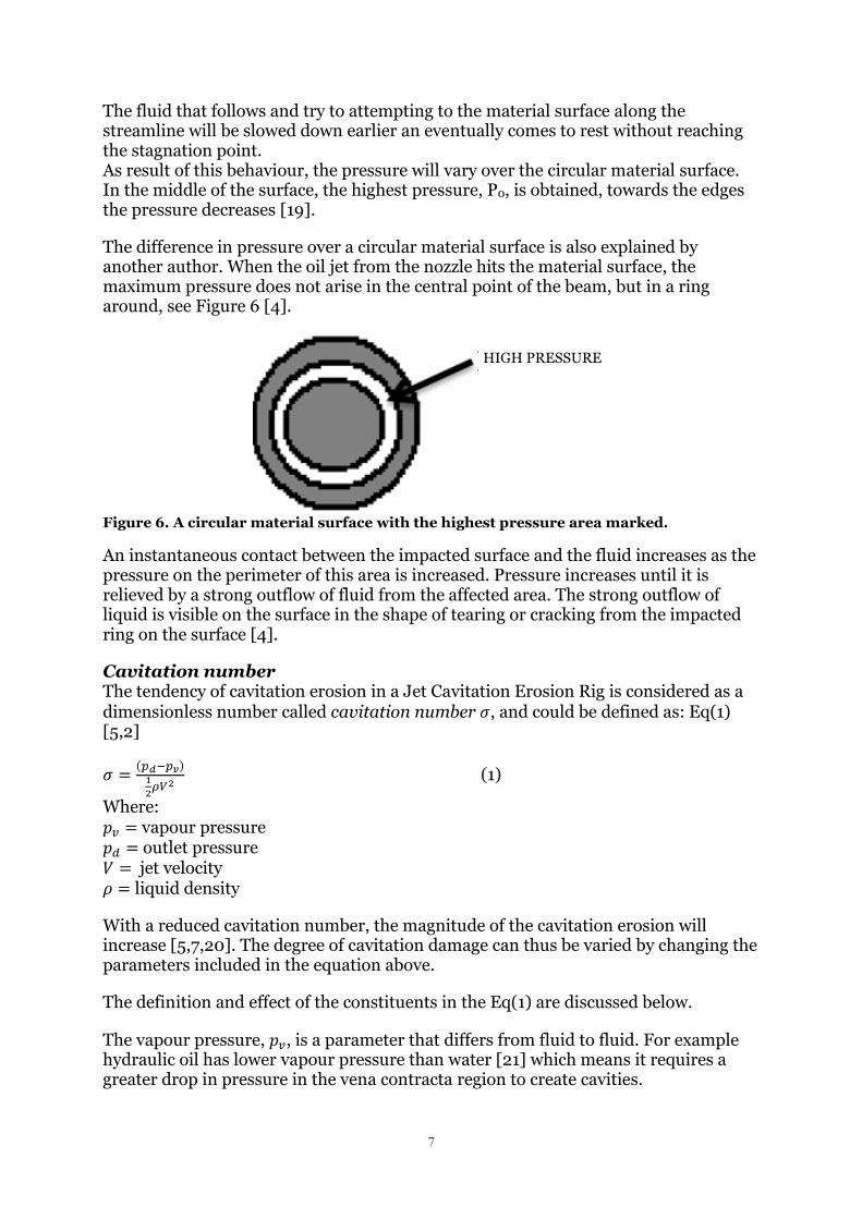
The difference in pressure over a circular material surface is also explained by another author. When the oil jet from the nozzle hits the material surface, the maximum pressure does not arise in the central point of the beam, but in a ring around, see Figure 6 [4].

HIGH PRESSURE

Figure 6. A circular material surface with the highest pressure area marked.

An instantaneous contact between the impacted surface and the fluid increases as the pressure on the perimeter of this area is increased. Pressure increases until it is relieved by a strong outflow of fluid from the affected area. The strong outflow of liquid is visible on the surface in the shape of tearing or cracking from the impacted ring on the surface [4].

Cavitation number The tendency of cavitation erosion in a Jet Cavitation Erosion Rig is considered as a dimensionless number called cavitation number , and could be defined as: Eq(1) [5,2]

(1)

Where: vapour pressure outlet pressure jet velocity liquid density

With a reduced cavitation number, the magnitude of the cavitation erosion will increase [5,7,20]. The degree of cavitation damage can thus be varied by changing the parameters included in the equation above.

The definition and effect of the constituents in the Eq(1) are discussed below.

The vapour pressure, , is a parameter that differs from fluid to fluid. For example hydraulic oil has lower vapour pressure than water [21] which means it requires a greater drop in pressure in the vena contracta region to create cavities.

8

The outlet pressure, , and its relation to inlet pressure controls the degree of drop in pressure that the fluid experience when it reached the chamber in the cavitation rig. A decreased outlet pressure, with a constant inlet pressure, gives a higher drop in pressure. This increases the probability that the local pressure in the vena contracta region gets lower than the vapour pressure, and thus generates more cavities.

The probability of cavitation damage increases with increasing velocity, , of the fluid [22,23] and the reason could be explained by higher risk of turbulence and pressure fluctuations in the fluid.

Liquid density, , varies between different liquids. With a higher liquid density the cavitation number in Equation (1) decreases.

Other tests have shown that the rate of growth and collapse of cavities depends on the viscosity [24]. A higher viscosity will, by vortices, suppress the local pressure drop areas [5].Higher viscosity, as in oil, gives a lower possibility for the cavities to grow, and thereby the lower effects of cavitation erosion [24].

Depending on the cavitation number the stand- off distance has to be adjusted. Stand-off distance, Eq (2), denotes the distance between the nozzle and the center on the surface of the sample in the cavitation rig. It is inversely proportional to the cavitation number, then the lower the cavitation number the longer the stand- off. This is explained by the growth of cavities in a cavitation rig requires time. If the fluid velocity is increased it requires a longer stand-off to give the cavities time to grow before impact of sample. The input parameters in the equation is detailed in APPENDIX I.

[2] (2)

9

3. EXPERIMENTAL DETAILS

3.1 Experimental set- up and equipment design

The specific rig built based on ASTM G134-95 and used in this thesis is shown in Figure 7. Inside the chamber the nozzle is seen on the left and the sample to the right, in between one can discern the cavitating jet. The oil has its inlet to the chamber to the left and its outlet on the upper side of the chamber. The connection attached on the down side of the chamber was only used as drainage.

Nozzle

Inlet

Outlet

Sample

Drainage

Figure 7. The cavitation rig built based on ASTM G134-95.

The nozzle in the rig was combined with a washer to simulate the nozzle recommended by the ATSM G134-95. In this way the orifice that gave rise to the vena contracta region is similar in shape as a stair, see Figure 8.

Figure 8. The nozzle (= 1 mm) and the washer (= 1,8 mm) used in the cavitation rig set up.

10

The cavitation rig was used with hydraulic oil as a fluid. The properties of the oil can be seen in Table 1.

Table 1. The physical properties of the hydraulic oil, Shell Tellus S2 V 46.

Property Value

Vapour pressure <0,5 Pa at 20ºC

Density 872 kg/m3 at 15ºC

Kinematic viscosity 46 mm2/s at 40ºC

During this investigation the inlet pressure, just before the nozzle, was controlled by the pump that supplied the system with hydraulic oil. The constant outlet pressure of approx. 2 bar was given by the resistance in the system. The tests were run at a temperature between 40- 60°C. The temperature was measured by a connected thermometer on the outlet oil and smoothed by a cooling system. Both the inlet pressure and the outlet pressure were measured by manometers on the incoming and outgoing oil.

Regarding variation of the cavitation number the only variable parameter in the tests were the jet velocity and the other parameters such as outlet pressure, vapour pressure and liquid density were constant.

Jet velocity variation was created through adjustment of the inlet pressure. By variation of the inlet pressure also the drop in pressure that the fluid experiences in the vena contracta region was varied even though the outlet pressure could not be changed.

The stand- off in the cavitation rig could be adjusted to be consistent with Eq (2).

3.1.1 Experiment design

In order to, in an appropriate way test whether the Jet Cavitation Erosion Rig reproduced cavitation erosion, the tests were divided into two separate sections.

1. A number of tests to find the parameters which produced the greatest material loss.

2. Identification of relative cavitation erosion resistance of the three bronzes with settings from 1.

3.2 Specification of selected materials

Three selected grades of copper alloy; aluminium bronze, tin bronze and leaded tin bronze used in this investigation are further presented.

Aluminum bronze is a copper alloy with 3- 15% Al and with addition of other alloying elements to modify the properties in the final shape [25]. Aluminum bronzes have the combination of high strength, excellent corrosion resistance and high wear resistance [25,26]. These alloys have also been shown to have good resistance against cavitation erosion.

Tin bronze normally contains 1,25- 10 % Sn and they always contains some amount of phosphorus [25]. The alloys have good corrosion resistance, moderate strength and

11

high conductivity [26]. The material has excellent formability and a high fatigue resistance [25]. They can also be cold drawn to increase the strength further as the material used in this study.

Leaded tin bronze are basically the same as tin bronze with the additional amount of lead. The advantage of adding lead into copper- base alloys are to improve the machinability, but mostly to get the excellent friction characteristics in e.g. bearing applications. However, it’s important to know that lead reduces both tensile strength and the ductility. When a cast structure is solidifying it creates dendrites due to different solidification temperatures. The spaces between the dendrites tend to form micro pores which is avoided by adding lead. In this way the casting is pressure- tight, which is important for fluid- handling applications [25].

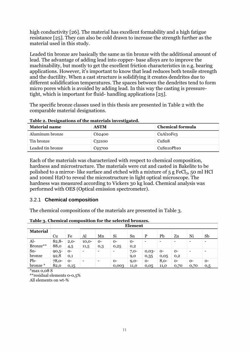
The specific bronze classes used in this thesis are presented in Table 2 with the comparable material designations.

Table 2. Designations of the materials investigated.

Material name ASTM Chemical formula

Aluminum bronze C62400 CuAl10Fe3

Tin bronze C52100 CuSn8

Leaded tin bronze C93700 CuSn10Pb10

Each of the materials was characterized with respect to chemical composition, hardness and microstructure. The materials were cut and casted in Bakelite to be polished to a mirror- like surface and etched with a mixture of 5 g FeCl3, 50 ml HCl and 100ml H2O to reveal the microstructure in light optical microscope. The hardness was measured according to Vickers 30 kg load. Chemical analysis was performed with OES (Optical emission spectrometer).

3.2.1 Chemical composition

The chemical compositions of the materials are presented in Table 3.

Table 3. Chemical composition for the selected bronzes. Element

Material Cu

Fe

Al

Mn

Si

Sn

P

Pb

Zn

Ni

Sb

Al- Bronze**

82,8- 88,0

2,0- 4,5

10,0- 11,5

0- 0,3

0- 0,25

0- 0,2

- - - - -

Sn- bronze

90,5- 92,8

0- 0,1

- - - 7,0- 9,0

0,03- 0,35

0- 0,05

0- 0,2

- -

Pb- bronze *

78,0- 82,0

0- 0,15

- - 0- 0,003

9,0- 11,0

0- 0,05

8,0- 11,0

0- 0,70

0- 0,70

0- 0,5

*max 0,08 S **residual elements 0-0,5% All elements on wt-%

12

3.2.2 Mechanical properties

The typical and measured mechanical properties are presented in Table 4.

Table 4. Typical properties of the selected bronzes [25].

Property

Material Rm [MPa]

Rp0,2/ Rp0,5 [MPa]

A5 [%]

Density [g/cm3]

Hardness [HV10]

Aluminum bronze 745 379 (Rp0,5) 12 7,45 200

Tin bronze 450 280 (Rp0,2) 15 8,86 130

Leaded tin bronze 450 350 >8 8,95 105

3.2.3 Microstructure

The microstructures of the three bronze alloys are presented in Figure 9.

As seen in the figure the aluminum bronze and the leaded tin bronze reveal a continuously cast condition with dendrites in the microstructure see Figure 9a and Figure 9c, while the tin bronze show a cold worked condition with slip bands, see Figure 9b. In the leaded tin bronze one can also see precipitations of lead as the dark spots.

13

a) b)

c)

Figure 9. Microstructure of polished and etched samples of the three bronzes (LOM). a) A dendritic microstructure of aluminum bronze, b) slip bands on a cold worked tin bronze and c) a dendritic microstructure of leaded tin bronze.

3.3 Sample preparation and geometry

All samples were machined to the dimensions as in Figure 10. Prior to test all the samples were polished. On the top of the surface on two specimens a hole of Ø=2,0 mm was drilled to perform a specific test described in the test parameters section.

Ø 12,0 mm

a)

3,8 mm

b) Figure 10. The dimensions of the samples used in this project. a) sample surface from the top and b) from the side.

14

3.4 Experimental procedures

After accomplishing the experiments at a desired time, the results were evaluated by the following:

The samples were washed with 1) dish soap, 2) ethanol bath in a ultrasonic cleaner, 3) dried in air.

The samples were weighted of an average of ten measurements where the mass loss was converted to volume loss according to ASTM G134. Volume loss was then used to determine accumulated volume loss and volume loss rate.

Microstructural examination using LOM. Note if no obvious volume loss at certain time was obtained an additional examination analysis were performed on cross- section samples.

Further analysis was accomplished using SEM and EDS to examine the eroded surface layer.

3.5 Characterization techniques

3.5.1 Weighing

The weighing equipment used to examine material loss during testing was an analytical balance. With a maximal capacity of 250g and a resolution of 0,1mg the equipment has a good precision.

3.5.2 Light Optical Microscopy

The Light Optical Microscope (LOM) is a microscopy technique used to characterize the microstructure of metallic materials. The LOM combines visible light and a system of lenses to create images of metallographic samples at high magnification. The lateral resolution and thus the maximum practical useful magnification of a modern LOM is restricted to 1.000x-1.500x because of the use of visible light. The limited depth of focus requires sample surfaces to be grinded and polished to reduce surface topography. Samples aimed for LOM are commonly etched to reveal the microstructure of the material [27].

3.5.3 Scanning Electron Microscopy

The Scanning Electron Microscope (SEM) can be used to create images in a wide range of magnifications, from about 100x to 500.000x, i.e. almost 500x times the practical useful magnification of a modern LOM. The large depth of focus in the SEM makes it possible to characterize even severely worn surfaces [27,28].

The SEM uses electrons to produce images of the samples. A focused electron beam of primary electrons is scanned in a line pattern over the sample surface to produce SEM micrographs. The characteristic three-dimensional appearance of the SEM micrographs is due to the narrow electron beam. The primary electrons interact with the atoms in the surface of the sample, which emits various signals that can be detected. The signals gives information about the sample´s surface topography and composition in a point- to- point image [29].

15

If the primary electrons collide inelastically with the sample surface they send out secondary electrons through the sample surface. Detection of secondary electrons is the most common detection mode and creates images where the brightness is proportional to the number of detected electrons. These images have a clear three- dimensional appearance and potentially high magnification. Primary electrons that collide elastically with the sample surface are emitted as backscattered electrons (BSE). The detection of backscattered electrons can be used in order to visualize chemical contrasts between different chemical compositions, phases, etc. Heavy elements (high atomic number) will result in a stronger BSE signal and consequently areas containing heavy elements will appear brighter [28].

3.5.4 Energy Dispersive X- ray Spectroscopy (EDS)

Scanning electron microscopy is commonly combined with energy dispersive X-ray spectroscopy (EDS). The EDS analytical technique is based on incoming primary electrons and emitted X-rays. By using an energy dispersive X-ray spectroscopy (EDS) detector, emitted characteristic X-rays can be detected and used to identify the composition of the sample and the distribution of different phases and elements in the sample using line-scan and mapping techniques. Since the number of emitted characteristic X-rays is related to the concentration of the corresponding element in the sample surface it is possible to obtain quantitative information about the chemical composition [28].

EDS can either take the form of point analysis, surface analysis, line scan or mapping. Mapping as is used in this work shows the distribution of the elements over the analysed area [29].

16

4. EVALUATION OF TEST PARAMETERS

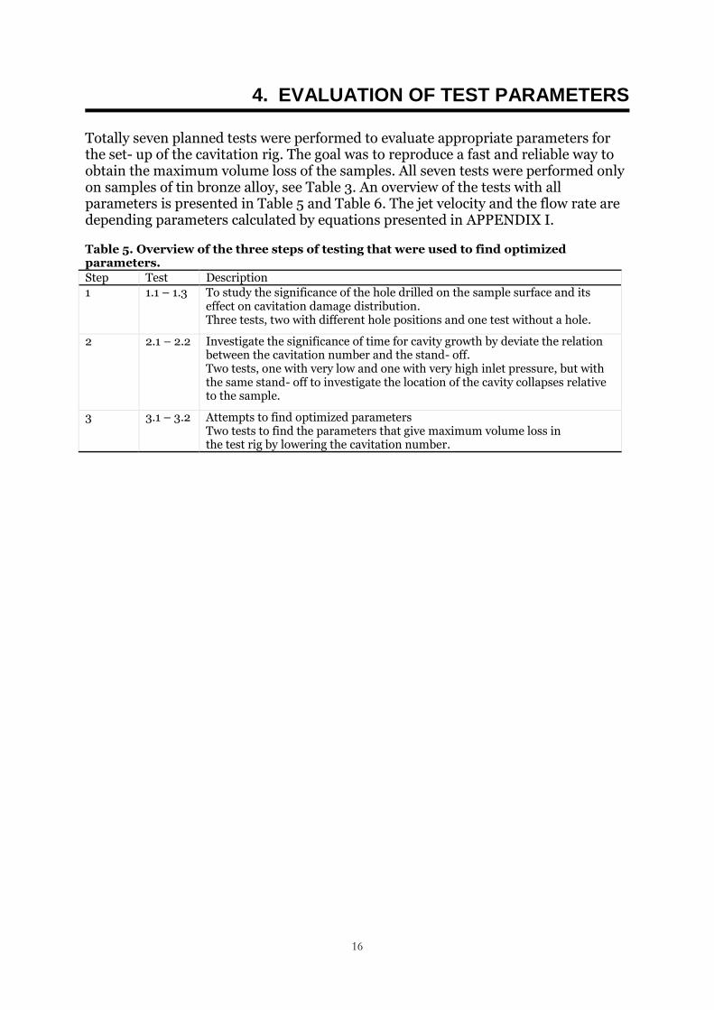
Totally seven planned tests were performed to evaluate appropriate parameters for the set- up of the cavitation rig. The goal was to reproduce a fast and reliable way to obtain the maximum volume loss of the samples. All seven tests were performed only on samples of tin bronze alloy, see Table 3. An overview of the tests with all parameters is presented in Table 5 and Table 6. The jet velocity and the flow rate are depending parameters calculated by equations presented in APPENDIX I.

Table 5. Overview of the three steps of testing that were used to find optimized parameters.

Step Test Description

1 1.1 – 1.3 To study the significance of the hole drilled on the sample surface and its effect on cavitation damage distribution. Three tests, two with different hole positions and one test without a hole.

2 2.1 – 2.2 Investigate the significance of time for cavity growth by deviate the relation between the cavitation number and the stand- off. Two tests, one with very low and one with very high inlet pressure, but with the same stand- off to investigate the location of the cavity collapses relative to the sample.

3 3.1 – 3.2 Attempts to find optimized parameters Two tests to find the parameters that give maximum volume loss in the test rig by lowering the cavitation number.

17

4.1 Experimental execution

Based on the parameters set up described in Table 6 different experiments steps were executed.

Table 6. The complete parameters for all tests to evaluate optimized parameters.

4.1.1 Step 1

The goal of these tests was to investigate the theories of the pressure over the sample surface [4,19]. The theories describes different location of the maximum pressure, thereby these tests were performed to evaluate where the cavities actually experienced maximum pressure and thus implode. The tests were made with one solid sample (Test1.1), one sample with centre hole (Test1.2) and one sample with a hole 4,5 mm from the centre (Test1.3). By the tests differences in volume loss- and

Parameter Test1.1 Test1.2 Test1.3 Test2.1 Test2.2 Test3.1 Test3.2

Nozzle diameter

1 1 1 1 1 1 1

Inlet pressure

157±1,0 157±1,0 157±1,0 75±1,0 250±1,0 188±1,0 243±1,0

Oulet pressure

2±0,5 2±0,5 2±0,5 2±0,5 2±0,5 2±0,5 2±0,5

Vapour pressure (20°C)

5∙10-6 5∙10-6 5∙10-6 5∙10-6 5∙10-6 5∙10-6 5∙10-6

Cavitation number *

≈0,0292 ≈0,0292 ≈0,0292 ≈0,0612 ≈0,0184 ≈0,0244 ≈0,0189

Jet velocity

127 127 127 88 160 139 158

Flow rate

9.96∙10-5 9.96∙10-5 9.96∙10-5 6.89∙10-5 9.96∙10-5 10.9∙10-5 12.4∙10-5

Stand-off

25,8±0,5 25,8±0,5 25,8±0,5 25,8±0,5 25,8±0,5 29,7±0,5 36,3±0,5

Test time

4 30 30 4 4 30 8

Hole placement from centre

NA 4,5 0 * NA NA NA NA

Bronze Tin Tin Tin Tin Tin Tin Tin

* hole is placed in the centre of the sample

18

rate between the samples with and without hole could be evaluated and compared. Details of the test parameters can be seen in Table 6.

4.1.2 Step 2

Tests were setup with two different cavitation numbers; due to low and high inlet pressure, but with the same initial stand- off. The aim was to verify the significance of the time for cavity growth and if the location for cavity collapses were related to the sample position based on the stand- off in Eq(2). In order to clearly see the difference in these tests a very low, 75 bar (Test2.1), and a very high, 250 bar (Test2.2), inlet pressure was used. The test parameters can be seen in Table 6.

4.1.3 Step 3

These tests were setup with aim to find parameters that reproduced a fast volume loss- and rate. To do this, a low cavitation number was calculated and applied in the stand- off equation in Eq(2) to select a stand- off that match the specific cavitation number (Test3.1). In the second test the cavitation number was calculated to be consistent with the maximum stand- off. The lowest possible cavitation number in accordance with Eq(1) and Eq(2) and the chamber was thus obtained (Test3.2). The size of the test chamber limit the maximum stand- off. See Table 6 for more parameter details.

4.2 Results and discussions

4.2.1 Step 1

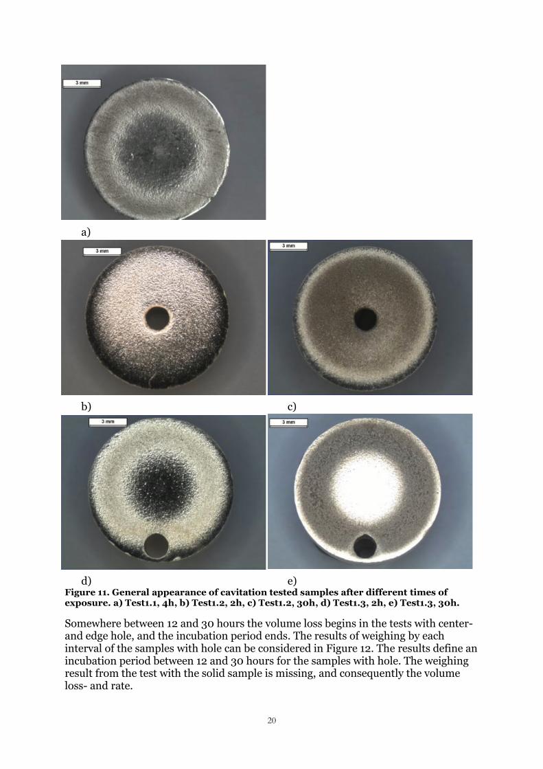
In the first test, without a hole in the sample, the cavitation damage appears at the periphery of the sample, see Figure 11a. The distribution of damage in the third test, with an edge hole, looks like the damage in the first test, see Figure 11d-e. This is on good agreement with the theory that the implosions of cavities tend to concentrate on the already damaged areas [8]. This theory was confirmed by the samples without a hole and with an edge hole where the damage seemed to be intensified in the early damaged areas.

As described in the theory there are differences between different sources and their description of the pressure over the sample surface [4,19]. To take both theories into account in connection they can be linked together with the distribution of the damage on the solid sample and thereby also on the sample with an edge hole. The small amount of pits seen in the center, in the stagnant point [19], could have arisen when the first oil reached the sample. But in this point only a few cavities reaches the sample surface before the oil stagnates. The circle along the edges where the majority of the damage can be seen can be connected to the theory which says that this is the area where the fluid and thus the cavities are exposed to the highest pressure [4]. Since the oil was in continued motion in this field, several cavities reached this area and thus collapse.

Also, a pronounced wear pattern can be observed in radial direction in the damaged area of the sample in Figure 11a. This is described in connection to the theory of the pressure distribution over the sample surface, where it was mentioned that some tearing can be seen from the damaged ring on the sample [4]. This kind of damage was only seen early in tests before the amount of damage increases.

19

Figure 11b-c shows that the damage is spread over the sample surface when using a center hole. This is because there was no stagnant point in the center of the sample, and thus the fluid was in motion all over the surface. It is possible that the pressure was more evenly distributed over the entire surface and the cavities were able to implode all over it. But by implosions spread all over the surface the concentrations of damage became lower, and thus it requires longer test times to reach the same level of volume loss as if the damage is concentrated.

20

a)

b) c)

d) e) Figure 11. General appearance of cavitation tested samples after different times of exposure. a) Test1.1, 4h, b) Test1.2, 2h, c) Test1.2, 30h, d) Test1.3, 2h, e) Test1.3, 30h.

Somewhere between 12 and 30 hours the volume loss begins in the tests with center- and edge hole, and the incubation period ends. The results of weighing by each interval of the samples with hole can be considered in Figure 12. The results define an incubation period between 12 and 30 hours for the samples with hole. The weighing result from the test with the solid sample is missing, and consequently the volume loss- and rate.

21

Figure 12. Accumulated volume loss versus time as displayed by the Sn-bronze in Test1.2 and Test1.3.

In the diagram it can be seen that the volume loss is much higher after 30 hours when the damage is concentrated to the edge of the sample (acc. volume loss 0,55 mm 3) using an edge hole compared to the test with centre hole (acc. volume loss 0,14 mm3). The corresponding volume loss rates at the end of the tests (i.e. based on the volume losses obtained after 12 and 30 hours) were found to be 0,005mm3/h and 0,018mm3/h for the center hole and edge hole samples, respectively.

The result from the tests showed that the hole in the centre of the sample caused damage on the whole surface area but it didn’t provide a faster volume loss rate than the sample with edge hole. The appearances of the damage on the samples with edge hole and without a hole were the same. Therefore it was decided to not use samples with holes in the future testing for a faster operation time (less lead time).

If deliberately concentration of the damage could be done by the choice of hole location, even the volume loss should be accelerated by such a choice. Since the sample with the edge hole and the solid sample suffered similar damage appearance the project was simplified by ignoring the additional moment that drilling of holes means.

4.2.2 Step 2

It was found that the damage differs a lot between the two tests, see Figure 13, but no volume loss was observed after four hours. The test with low inlet pressure in relation to the stand- off showed a few pits in the center of the sample, see Figure 13a, while the test with higher inlet pressure was more heavily damaged on the edge, see Figure 13b. The damage on the sample tested with low inlet pressure is most likely due to the small pressure drop which generates fewer cavities. The damage on the sample tested with high inlet pressure is most likely due to the short time for cavity growth.

-0,1

0

0,1

0,2

0,3

0,4

0,5

0,6

0 1 10 100

Acc

um

ula

ted

vo

lum

e lo

ss [

mm

3]

Time [log(h)]

Test1.2 accumulated volume loss, centerhole

Test1.3 accumulated volume loss, edge hole

22

According to Eq(2) the stand- off should be adjusted with respect to the selected inlet pressure. But the stand- off was fixed in these both tests. Since the inlet pressure was low in the first test the cavities must have been fewer, due to low pressure drop. Larger in size due to the longer time to expand but may have imploded before they actually hit the sample surface. In the second test many of the cavities may have missed the sample due to higher velocity and flow rate of the fluid. However this test showed almost the same damaged appearance as Test1.1, which means that an amount of the cavities must have imploded on the surface. This indicates that a larger amount of smaller cavities gave almost the same damages as a smaller amount of cavities of desired size. But the higher inlet pressure and velocity provides major wear on the cavitation rig. Therefore, it is desirable to keep to the equations, Eq(1) and Eq(2), and create cavitation damages with these as a starting point.

The outcome of this result verified that the equations of the cavitation number and the stand- off were consistent with the behaviour of the specific cavitation rig.

a) b) Figure 13. General appearance of cavitation tested samples after four hours of exposure. Where a) shows Test2.1 with inlet pressure 75 bar and b) Test2.2 with inlet pressure 250 bar.

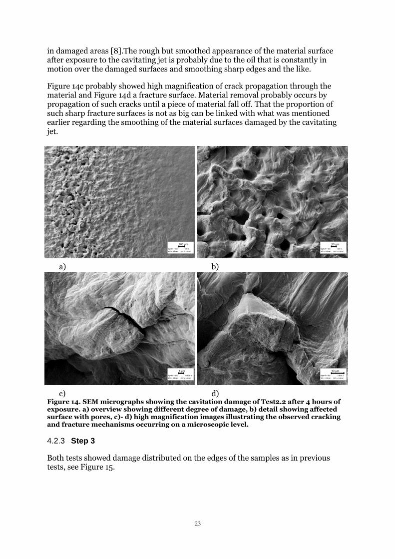
The surface of the test with high inlet pressure after 4 hours exposure was investigated with SEM, the images is shown in Figure 14. The surface was plastically deformed but the deformation differed over the surface area, where the most affected areas were at the edge.

In Figure 14a two degrees of damages could be seen. According to the image the sample seems to, at least in tin bronze, be plastically deformed initially. Upon further exponation of implosions the surface becomes more and more rough but smoothed in the middle of the same image. Finally voids are formed due to micro jets and shockwaves, to the left in the image, and volume loss begins. That all these degrees of damage could be seen simultaneously on a single sample could be linked to the spread and concentrations of cavity implosions [8]. Implosions probably took place over the whole, more or less, damaged sample but the severe the damage was, the more concentrated the implosions had been.

Figure 14b shows voids in higher resolution. Those voids arose in the damaged ring of the sample where the pressure is highest [4], and thus in the area where the damage concentrates maybe also to some extent due to lower resistance to cavitation erosion

23

in damaged areas [8].The rough but smoothed appearance of the material surface after exposure to the cavitating jet is probably due to the oil that is constantly in motion over the damaged surfaces and smoothing sharp edges and the like.

Figure 14c probably showed high magnification of crack propagation through the material and Figure 14d a fracture surface. Material removal probably occurs by propagation of such cracks until a piece of material fall off. That the proportion of such sharp fracture surfaces is not as big can be linked with what was mentioned earlier regarding the smoothing of the material surfaces damaged by the cavitating jet.

Figure 14. SEM micrographs showing the cavitation damage of Test2.2 after 4 hours of exposure. a) overview showing different degree of damage, b) detail showing affected surface with pores, c)- d) high magnification images illustrating the observed cracking and fracture mechanisms occurring on a microscopic level.

4.2.3 Step 3

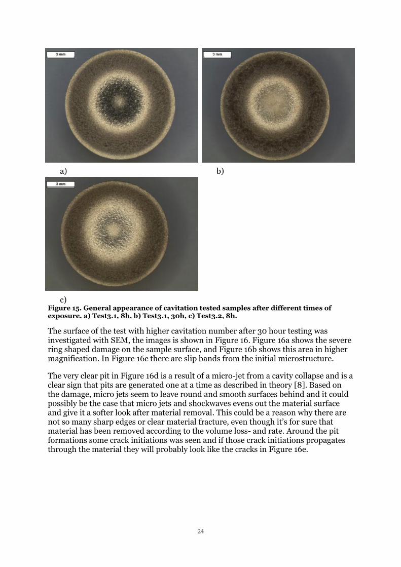
Both tests showed damage distributed on the edges of the samples as in previous tests, see Figure 15.

a) b)

c) d)

24

a) b)

c)

Figure 15. General appearance of cavitation tested samples after different times of exposure. a) Test3.1, 8h, b) Test3.1, 30h, c) Test3.2, 8h.

The surface of the test with higher cavitation number after 30 hour testing was investigated with SEM, the images is shown in Figure 16. Figure 16a shows the severe ring shaped damage on the sample surface, and Figure 16b shows this area in higher magnification. In Figure 16c there are slip bands from the initial microstructure.

The very clear pit in Figure 16d is a result of a micro-jet from a cavity collapse and is a clear sign that pits are generated one at a time as described in theory [8]. Based on the damage, micro jets seem to leave round and smooth surfaces behind and it could possibly be the case that micro jets and shockwaves evens out the material surface and give it a softer look after material removal. This could be a reason why there are not so many sharp edges or clear material fracture, even though it’s for sure that material has been removed according to the volume loss- and rate. Around the pit formations some crack initiations was seen and if those crack initiations propagates through the material they will probably look like the cracks in Figure 16e.

25

a) b)

c) d)

e)

Figure 16. SEM micrographs showing the damage of Test3.1 after 30 hours of exposure where a)shows an overview of the damaged surface, b) the damage in higher magnification, c) slip bands, d) pit and e) cracks on the surface. Images are of tilted view.

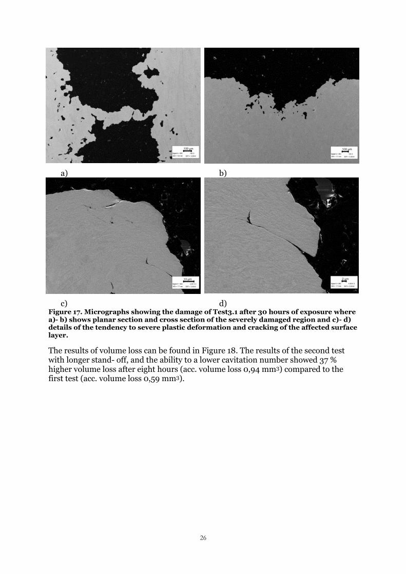
To more clearly see how the damage propagates inside the material planar and cross sections of the sample were investigated, see Figure 17. It can be identified that the worn area exhibit severe plastic deformation and the cracks seen in the cross section indicate cracks propagate downwards in the material. Cracks that meet tend to lead to material removal and voids in the material surface.

26

a) b)

c) d) Figure 17. Micrographs showing the damage of Test3.1 after 30 hours of exposure where a)- b) shows planar section and cross section of the severely damaged region and c)- d) details of the tendency to severe plastic deformation and cracking of the affected surface layer.

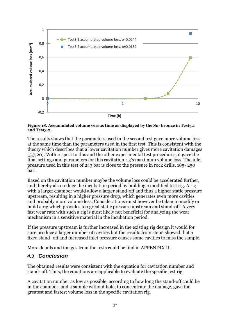
The results of volume loss can be found in Figure 18. The results of the second test with longer stand- off, and the ability to a lower cavitation number showed 37 % higher volume loss after eight hours (acc. volume loss 0,94 mm3) compared to the first test (acc. volume loss 0,59 mm3).

27

Figure 18. Accumulated volume versus time as displayed by the Sn- bronze in Test3.1 and Test3.2.

The results shows that the parameters used in the second test gave more volume loss at the same time than the parameters used in the first test. This is consistent with the theory which describes that a lower cavitation number gives more cavitation damages [5,7,20]. With respect to this and the other experimental test procedures, it gave the final settings and parameters for this cavitation rig’s maximum volume loss. The inlet pressure used in this test of 243 bar is close to the pressure in rock drills, 185- 250 bar.

Based on the cavitation number maybe the volume loss could be accelerated further, and thereby also reduce the incubation period by building a modified test rig. A rig with a larger chamber would allow a larger stand-off and thus a higher static pressure upstream, resulting in a higher pressure drop, which generates even more cavities and probably more volume loss. Considerations must however be taken to modify or build a rig which provides too great static pressure upstream and stand-off. A very fast wear rate with such a rig is most likely not beneficial for analyzing the wear mechanism in a sensitive material in the incubation period.

If the pressure upstream is further increased in the existing rig design it would for sure produce a larger number of cavities but the results from step2 showed that a fixed stand- off and increased inlet pressure causes some cavities to miss the sample.

More details and images from the tests could be find in APPENDIX II.

4.3 Conclusion

The obtained results were consistent with the equation for cavitation number and stand- off. Thus, the equations are applicable to evaluate the specific test rig.

A cavitation number as low as possible, according to how long the stand-off could be in the chamber, and a sample without hole, to concentrate the damage, gave the greatest and fastest volume loss in the specific cavitation rig.

-0,2

0

0,2

0,4

0,6

0,8

1

0 1 10

Acc

um

ula

ted

vo

lum

e lo

ss [

mm

3 ]

Time [h]

Test3.1 accumulated volume loss, σ=0,0244

Test3.2 accumulated volume loss, σ=0,0189

28

For future tests the erosion rate can probably be further increased, and thereby decreasing the test times by constructing a similar test rig with the possibility of a larger stand-off.

Based on the fact that the appearances of the damage in many cases were consistent with the description of cavitation damage it was concluded that the Jet Cavitation Erosion Rig produced cavitation damage.

29

5. RELATIVE CAVITATION RESISTANCE

5.1 Experimental execution

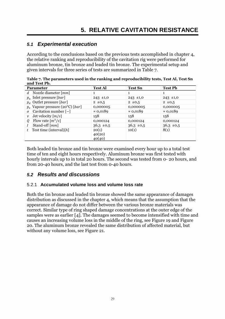
According to the conclusions based on the previous tests accomplished in chapter 4, the relative ranking and reproducibility of the cavitation rig were performed for aluminum bronze, tin bronze and leaded tin bronze. The experimental setup and given intervals for three series of tests are summarized in Table 7.

Table 7. The parameters used in the ranking and reproducibility tests, Test Al, Test Sn and Test Pb.

Parameter Test Al Test Sn Test Pb

Nozzle diameter 1 1 1

Inlet pressure 243 ±1,0 243 ±1,0 243 ±1,0

Outlet pressure 2 ±0,5 2 ±0,5 2 ±0,5

Vapour pressure (20°C) 0,000005 0,000005 0,000005

Cavitation number ≈ 0,0189 ≈ 0,0189 ≈ 0,0189

Jet velocity 158 158 158

Flow rate 0,000124 0,000124 0,000124

Stand-off 36,3 ±0,5 36,3 ±0,5 36,3 ±0,5

Test time (interval) 20(1) 40(20) 40(40)

10(1) 8(1)

Both leaded tin bronze and tin bronze were examined every hour up to a total test time of ten and eight hours respectively. Aluminum bronze was first tested with hourly intervals up to in total 20 hours. The second was tested from 0- 20 hours, and from 20-40 hours, and the last test from 0-40 hours.

5.2 Results and discussions

5.2.1 Accumulated volume loss and volume loss rate

Both the tin bronze and leaded tin bronze showed the same appearance of damages distribution as discussed in the chapter 4, which means that the assumption that the appearance of damage do not differ between the various bronze materials was correct. Similar type of ring shaped damage concentrations at the outer edge of the samples were as earlier [4]. The damages seemed to become intensified with time and causes an increasing volume loss in the middle of the ring, see Figure 19 and Figure 20. The aluminum bronze revealed the same distribution of affected material, but without any volume loss, see Figure 21.

30

a) b) Figure 19. The evolution of the damage in leaded tin bronze. a) after one hour of testing and b) after eight hours of testing.

a) b) Figure 20. The evolution of the damage in tin bronze. a) after one hour of testing and b) after ten hours of testing.

31

a) b)

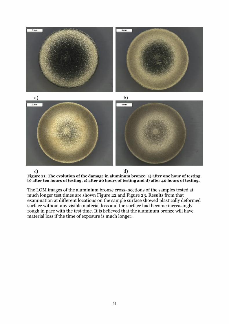
c) d) Figure 21. The evolution of the damage in aluminum bronze. a) after one hour of testing, b) after ten hours of testing, c) after 20 hours of testing and d) after 40 hours of testing.

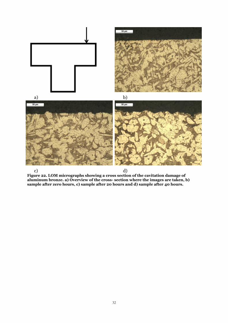
The LOM images of the aluminium bronze cross- sections of the samples tested at much longer test times are shown Figure 22 and Figure 23. Results from that examination at different locations on the sample surface showed plastically deformed surface without any visible material loss and the surface had become increasingly rough in pace with the test time. It is believed that the aluminum bronze will have material loss if the time of exposure is much longer.

32

a) b)

c) d) Figure 22. LOM micrographs showing a cross section of the cavitation damage of aluminum bronze. a) Overview of the cross- section where the images are taken, b) sample after zero hours, c) sample after 20 hours and d) sample after 40 hours.

33

a) b)

c) d) Figure 23. LOM micrographs showing the plastically deformation on the edge (bow out) of the aluminum bronze samples. a) overview of the cross- section where the images are taken, b) non- deformed sample after zero hours, c) sample after 20 hours and d) sample after 40 hours.

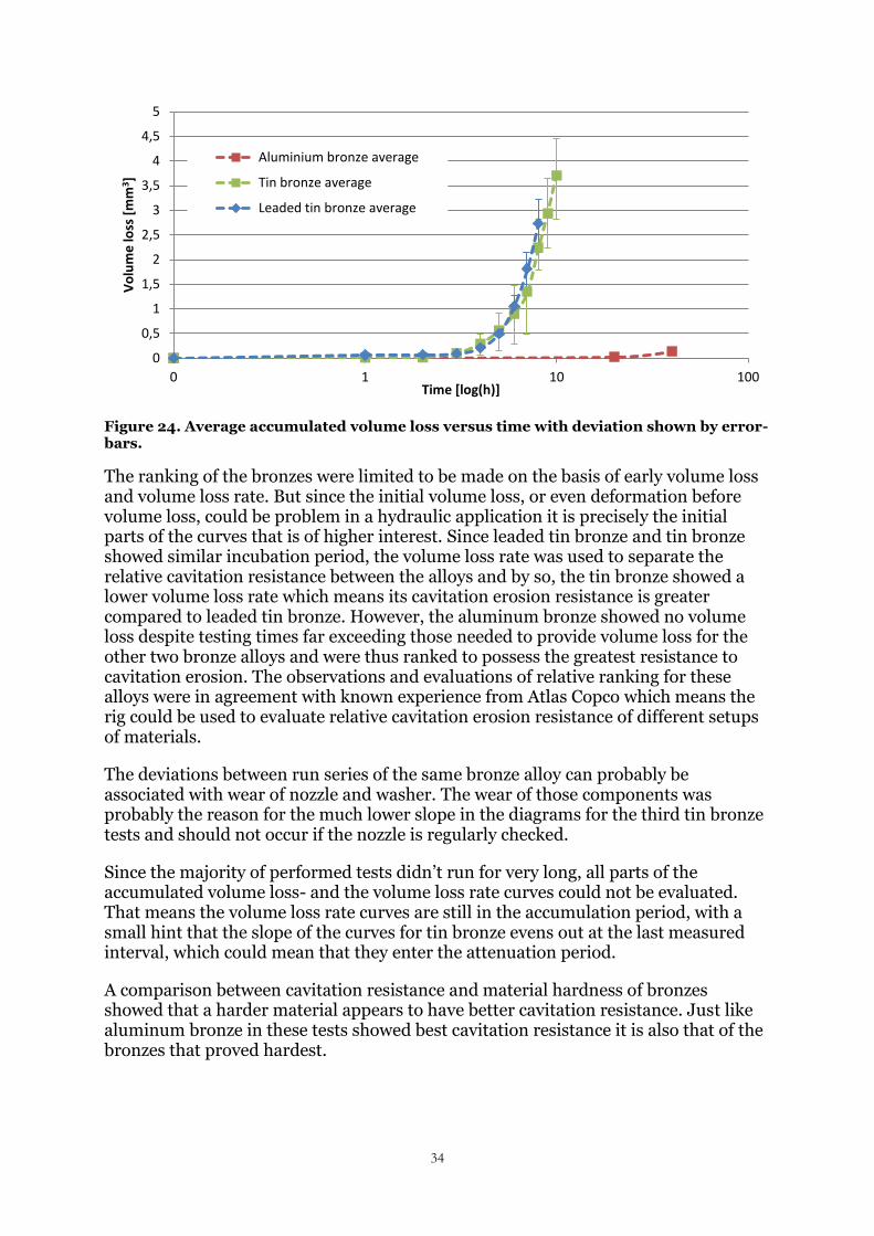
In the volume loss diagram, Figure 24, it could be seen that the volume loss started somewhere between two and three hours, for tin bronze and leaded tin bronze, after which it increased exponentially, in accordance with step2 presented in Figure 2 [30]. For the tin bronze, the small hint that the slope of the curve turned of slightly between nine and ten hours could mean the curve was about to pass into the linearly increasing region presented as step3 in Figure 2 [30]. For the leaded tin bronze there was no indications for a reduced slope, it was therefore still in step2.

The volume loss rate curves for tin bronze and leaded tin bronze passed from incubation period to accumulation period between two and three hours. The volume loss rate was 0,3423 mm3/h for leaded tin bronze and 0,2806 mm3/h for tin bronze after eight hours and 0,00347 mm3/h for aluminum bronze after 40 hours.

No incubation period was observed for the aluminum bronze. Accumulated volume loss- and rate were higher for the leaded tin bronze than for the tin bronze, see Figure 24 where all three bronze alloys are compared. Pursuant to this, aluminium bronze were ranked as the most resistant material to cavitation erosion, followed by tin bronze and last the leaded tin bronze.

34

Figure 24. Average accumulated volume loss versus time with deviation shown by error- bars.

The ranking of the bronzes were limited to be made on the basis of early volume loss and volume loss rate. But since the initial volume loss, or even deformation before volume loss, could be problem in a hydraulic application it is precisely the initial parts of the curves that is of higher interest. Since leaded tin bronze and tin bronze showed similar incubation period, the volume loss rate was used to separate the relative cavitation resistance between the alloys and by so, the tin bronze showed a lower volume loss rate which means its cavitation erosion resistance is greater compared to leaded tin bronze. However, the aluminum bronze showed no volume loss despite testing times far exceeding those needed to provide volume loss for the other two bronze alloys and were thus ranked to possess the greatest resistance to cavitation erosion. The observations and evaluations of relative ranking for these alloys were in agreement with known experience from Atlas Copco which means the rig could be used to evaluate relative cavitation erosion resistance of different setups of materials.

The deviations between run series of the same bronze alloy can probably be associated with wear of nozzle and washer. The wear of those components was probably the reason for the much lower slope in the diagrams for the third tin bronze tests and should not occur if the nozzle is regularly checked.

Since the majority of performed tests didn’t run for very long, all parts of the accumulated volume loss- and the volume loss rate curves could not be evaluated. That means the volume loss rate curves are still in the accumulation period, with a small hint that the slope of the curves for tin bronze evens out at the last measured interval, which could mean that they enter the attenuation period.

A comparison between cavitation resistance and material hardness of bronzes showed that a harder material appears to have better cavitation resistance. Just like aluminum bronze in these tests showed best cavitation resistance it is also that of the bronzes that proved hardest.

0

0,5

1

1,5

2

2,5

3

3,5

4

4,5

5

0 1 10 100

Vo

lum

e lo

ss [

mm

3 ]

Time [log(h)]

Aluminium bronze average

Tin bronze average

Leaded tin bronze average

35

5.2.2 SEM- and EDS analysis of damages

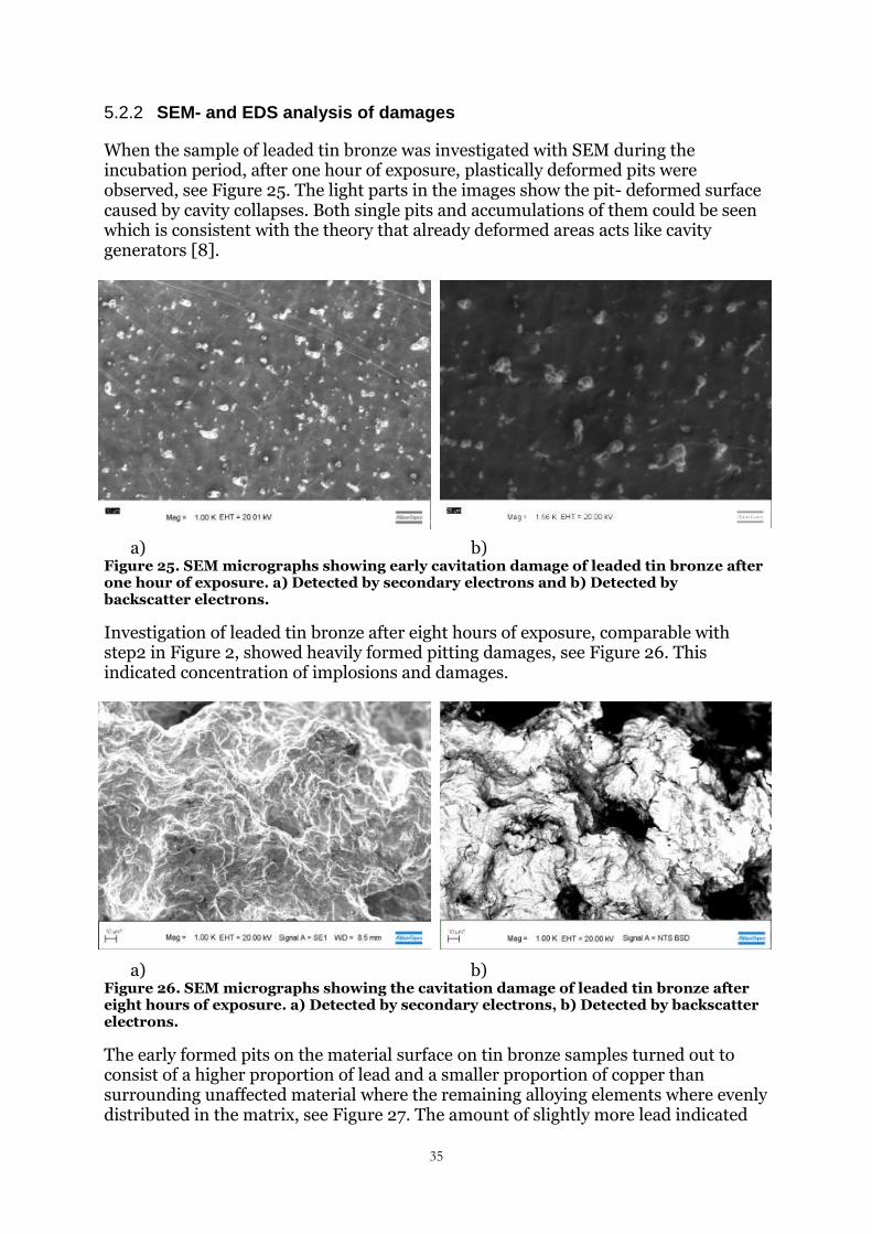
When the sample of leaded tin bronze was investigated with SEM during the incubation period, after one hour of exposure, plastically deformed pits were observed, see Figure 25. The light parts in the images show the pit- deformed surface caused by cavity collapses. Both single pits and accumulations of them could be seen which is consistent with the theory that already deformed areas acts like cavity generators [8].

a) b) Figure 25. SEM micrographs showing early cavitation damage of leaded tin bronze after one hour of exposure. a) Detected by secondary electrons and b) Detected by backscatter electrons.

Investigation of leaded tin bronze after eight hours of exposure, comparable with step2 in Figure 2, showed heavily formed pitting damages, see Figure 26. This indicated concentration of implosions and damages.

a) b) Figure 26. SEM micrographs showing the cavitation damage of leaded tin bronze after eight hours of exposure. a) Detected by secondary electrons, b) Detected by backscatter electrons.

The early formed pits on the material surface on tin bronze samples turned out to consist of a higher proportion of lead and a smaller proportion of copper than surrounding unaffected material where the remaining alloying elements where evenly distributed in the matrix, see Figure 27. The amount of slightly more lead indicated

36

that the lead was not quite evenly distributed over the surface of the material, but seen as precipitations as mentioned in Figure 9. The lead precipitations are softer than the other surrounding alloying elements and seemed to primarily be damaged by the cavity collapses. The longer the test time the less clearly became the slightly uneven distribution.

Leaded tin bronze Overview Cu Sn Pb

0h

3

2h

4h

6h

8h

Figure 27. EDS analysis of the main elements in leaded tin bronze after different times of exposure.

When the tin bronze samples were investigated during the incubation period, after one hour, they also showed plastically deformed pits, see Figure 28. The images in Figure 29 show the damage after two and ten hours. After two hours, Figure 29a-b, the volume loss had not started but the surface was heavily damaged and looks similar to the damage after ten hours, Figure 29c-d. However, there was a clear difference between the voids. They were much deeper after ten hours of exposure when the volume loss, step2 in Figure 2, had been proceeding some hours.

37

a) b) Figure 28. SEM micrographs showing the early cavitation damages of tin bronze after one hour of exposure. a) Detected by secondary electrons, b) Detected by backscatter electro ns.

a) b)

c) d) Figure 29. SEM micrographs showing the cavitation damage of tin bronze after two and ten hours of exposure. a) Detected by secondary electrons after two hours of exposure, b) Detected by backscatter electrons after two hours of exposure, a) Detected by secondary electrons after ten hours of exposure and d) Detected by backscatter electrons after ten hours of exposure.

38

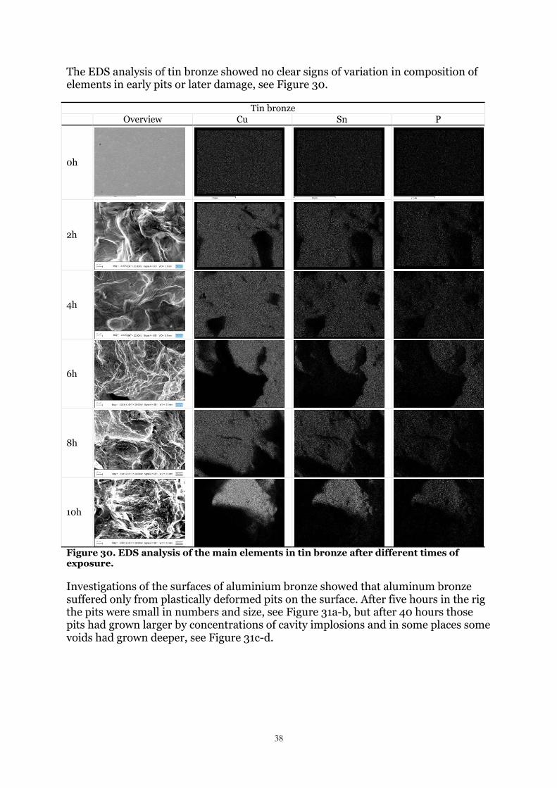
The EDS analysis of tin bronze showed no clear signs of variation in composition of elements in early pits or later damage, see Figure 30.

Tin bronze Overview Cu Sn P

0h

2h

4h

6h

8h

10h

Figure 30. EDS analysis of the main elements in tin bronze after different times of exposure.

Investigations of the surfaces of aluminium bronze showed that aluminum bronze suffered only from plastically deformed pits on the surface. After five hours in the rig the pits were small in numbers and size, see Figure 31a-b, but after 40 hours those pits had grown larger by concentrations of cavity implosions and in some places some voids had grown deeper, see Figure 31c-d.

39

a) b)

c) d) Figure 31. SEM micrographs showing the cavitation damage of aluminum bronze. a) Detected by secondary electrons after five hours, b) Detected by backscatter electrons after five hours, c) Detected by secondary electrons after 40 hours and b) Detected by backscatter electrons after 40 hours.

On the aluminum bronze it seemed to be a slightly less contents of aluminum in the damaged areas, see Figure 32. This, in contrast to the leaded tin bronze should imply that aluminium which has higher hardness than lead and seemed to resist the cavitation damage more than lead itself. Such an observation as the difference between lead and aluminum alloying elements was not observed in the tin bronze.

40

Aluminum bronze Overview Cu Fe Al

0h

2h

4h

40h

Figure 32. EDS analysis of the main elements in aluminum bronze after different times of exposure.

Common for all SEM investigations was that the longer the testing time passes, the less distinct becomes each pit. This agrees with the description in the theory that pits tend to concentrate since already formed pits acts like “cavitation generators” [8].

More details and images from the tests could be find in APPENDIX III

5.3 Conclusion

The repeatability was relatively good and the expected ranking was found. This means that the cavitation rig is fulfilling its purpose to be able to use in further investigations of new materials and can therefore be used on Atlas Copco Rock drills AB

The present cavitation erosion testing technique has proven very fruitful when it comes to evaluate the wear resistance of different materials exposed to cavitation erosion.

Also, the small size of the samples facilitates post-test characterization by microscopy and surface analysis generating detailed information of the prevailing surface failure mechanisms.

41

6. FUTURE WORK

Some suggestions for future tests, in addition to compare the degree of cavitation resistance of new materials in relation to already known.

By modifying the current cavitation rig, or construct a new one, to increase the chamber and hence allow a longer stand- off and a lower cavitation number the testing times to reach volume loss of various materials could be shortened. Perhaps tests that reach all the way to steady state in the volume loss curve can be done during reasonable periods of time.

Cavitation damage has been shown to concentrate in already damaged areas. It may be interesting to examine how the sensitivity of cavitation varies with the roughness of the material. Perhaps a initially damaged material surface provokes cavitation damage.

To provide a picture of how the material is likely to behave in a rock drill, with regard to cavitation, it may be interesting to extrapolate the results from the cavitation rig to a timescale for a real rock drill.

Examine how the damage and material removal occurs, and if there are any changes in the structures.

42

7. REFERENCES

[1] Timo Koivula, "On Cavitation in Fluid Power," Tampere University of Technology, Finland,.

[2] ASTM International G134-95, Standard Test Method for Erosion of Solid Materials by Cavitating Liquid Jet., updated December2010.

[3] Arvind Jayaprakash, Georges L. Chahine Jin-Keun Choi, "Scaling of Cavitation Erosion Progression with Cavitation Intensity and Cavitation Source," Wear, no. 278-279, pp. 53-61, January 2012.

[4] Frederick G. Hammit, "Liquid Erosion Failures," in ASM Handbook 11, Failure analysis and prevention.: ASM International, The Materials Information Society, 1986.

[5] D.K. Wills, D.G. Feldmann G.E. Totten, Hydraulic Failure Analysis: Fluids, Components, and System Effects.: ASTM International - Standards worldwide, ASTM Stock Number: STP1339.

[6] Li Jiang, Chen Darong, Wang Jiadao Chen Haosheng, "Damages on Steel Surface at the Incubaion Stage of the Vibration Cavitation Erosion in Water," Science Direct, vol. 265, pp. 692-698, February 2008.

[7] Bernd Bachert, Bernd Stoffel, Brane Sirok Matevz Dular, "Relationship between Cavitation Structures and Cavitation Damage," Science Direct, vol. 257, pp. 1176-1184, October 2004.

[8] Aljaz Osterman Matevz Dular, "Pit Clustering in Cavitation Erosion," Wear, vol. 265, pp. 811-820, March 2008.

[9] Shengcai Li Yoshiro Iwai, "Cavitation Erosion in Waters having Different Surface Tensions," Wear, vol. 254, pp. 1-9, September 2003.

[10] Alfred J. Crosby Jessica A. Zimberlin, "Water Cavitation of Hydrogels," Department of Polymer Science and Engineering, University of Massachusetts, Amherst, Massachusetts, 2009.

[11] Meghan O´Meara, "Determination of the Interfacial Tension between Oil-Steam and Oil-Air at Elevated Temperatures," North Carolina State University, Raleigh, North Carolina, 2012.

[12] I. Sam Saquy Dina Dana, "Review: Mechanism of oil uptake during deep-fat frying and the surfactant effect-theory and myth," Advances in Colloid and Interface Science, vol. 128-130, pp. 267-272, December 2006.

[13] Johnny Österman Carl Nordling, Physics Handbook for Science and Engineering, 8th ed. Lund, Sweden: Studentlitteratur, 2008.

[14] M. Szkodo, "Mathematical Description and Evaluation of Cavitation Erosion Resistance of Materials," Faculty of Mechanical Engineering, Gdansk University of Technology, Poland,.

[15] F.T. Cheng, H.C. Man K.Y. Chiu, "Evolution of Surface Roughness of some Metallic Materials in Cavitation Erosion," Science direct, vol. 43, pp. 713-716, April 2005.

[16] Tsunenori Okada, Yoichiro Baba Kichiro Endo, "Fundamental Studies on Cavitation Erosion," Japan, 1969.

[17] Queen´s University, Canada, Inge L.H. Hansson, Alcan International Ltd., Canada Carolyn M. Hansson, Cavitation Erosion, in ASM Handbook Volume 18 Friction, Lubrication, and Wear Technology. Canada: ASM International, The

43

Materials Information Society, 1992.

[18] B.S. Massey, Mechanics of Fluids, 5th ed. United Kingdom: Van Nostrand Reinhold (UK) Co. Ltd, 1983.

[19] (2014-04-03) Princeton. [Online]. http://www.princeton.edu/~asmits/Bicycle_web/Bernoulli.html

[20] Matevz Dular Martin Petkovsek, "Simultaneous Observation of Cavitationg Structures and Cavitation Erosion," Wear, vol. 300, pp. 55-64, February 2013.

[21] E.C. Fitch. (2014-04-23) Machinerylubrication. [Online]. http://machinerylubrication.com/Read/380/cavitation-wear-hydraulic

[22] Bernd Stoffel, Brane Sirok Matevz Dular, "Development of a Cavitation Erosion Model," Wear, vol. 261, pp. 642-655, February 2006.

[23] C.H. Venner, W.E. ten Napel Y. Meged, "Classification of Lubricants According to Cavitation Criteria," Wear, vol. 186-187, pp. 444-453, 1995.

[24] D.J. Hargreaves R. Pai, "Performance of Environment-Friendly Hydraulic Fluids and Material Wear in Cavitating Conditions," Wear, vol. 252, pp. 970-978, April 2002.

[25] Davis & Associates J.R. Davis, ASM Specialty Handbook, Copper and Copper Alloys.: ASM International, 2001.

[26] Metallnormcentralen, MNC Handbok nr8 Koppar och kopparlegeringar, 2nd ed., MNC-publikation, Ed. Sverige: SIS, september 1987.

[27] R. Hellborg, HJ. Whitlow, O. Hunderi D. Brune, Surface Characterization - A User's Sourcebook., 1997.

[28] J. Goldstein, Scanning Electron Microscopy and X-ray Microanalysis.: Kluwer Academic / Plenum Publishers, 2003.

[29] Staffan Jacobson, Åsa Kassman- Rudolphi Sture Hogmark, Svepelektronmikroskopi i praktik och teori, 9th ed.: Ångströmslaboratoriet Uppsala Universitet, 2006.

[30] Aljaz Osterman Matevz Dular, "Pit clustering in cavitation erosion," Wear, vol. 265, pp. 811-820, March 2008.

[31] Sture Hogmark Staffan Jacobson, Tribologi- Friktion, Smörjning, Nötning. Uppsala: Uppsala Universitet- Ångströmslaboratoriet, 2005.

[32] Olof Olsson m.fl. Linköpings tekniska Högskola, Kompendium i hydraulik, LiTH-IKP-S-316.

[33] T. Kazama Atsushi Yamaguchi, "Effects of Configuration of Nozzles, Outlet of Nozzles and Specimens on Erosion Due to Impingement of Cavittating Jet," Institute of Technology, Presented at the International Exposition for Power Transmission and Technical Conference, 4-6 April 2000.

[34] Joseph R. Davis, Consice Metals Engineering Data Book.: ASM International, 1997.

[35] McGraw-Hill Companies. (2014-02-27) Encyclopedia. [Online]. http://encyclopedia2.thefreedictionary.com/Cavitation

[36] Bernd Bachert, Brane Sirok, Matevz Dular Aljaz Osterman, "Time dependent measurements of cavitation damage," Wear, vol. 266, pp. 945-951, December 2008.

[37] J.D. Bressan, M.A. Klemz G. Basanini, "Cavitation erosion wear of metallic specimens using the new compact rotating disk device," Santa Catarina state

44

university- udesc joinville, department of mechanical engineering, Brazil,.

[38] (2014-04-03) [Online]. http://en.wikipedia.org/wiki/Pump

[39] Andrew W. Batchelor Gwidon W. Stachowiak, Engineering tribology, 3rd ed. Burlington, MA, USA: Butterworth- Heinemann, 2005.

[40] Boleslaw Giren, Janusz Steller Edyta Jurewicz, "Cavitation erosion - a possible cause of the mass loss within thrust in the Tatra Mts.," Acta Geologica Polonica, vol. 57, no. 2, pp. 305-323, 2007.

[41] A. Toro L.A. Espita, "Cavitation Resistance, Microstructure and Surface Topography of Materials used for Hydraulic Components," Tribology International, vol. 43, pp. 2037-2045, May 2010.

[42] Zhu Jirrhua Long Nrdong, "Cavitation Erosion Resistance and Ratio of Elastic Deformation Energy for Ti3Al and TiNiNb Alloys," State Key Laboratory for Mechanical Behavior of Materials, Xi an Jiaotong university, China, 2004.

[43] Andreas Malmlöf, "Optimising Material Testing Equipment for Maximum Cavitation," Atlas Copco Rock drills AB, Örebro,.

[44] Ida Masato, "Multibubble Cavitation Inception," Center for Computational Sceience and E-systems, Japan Atomic Energy Agency, Tokyo, 2009.

[45] Janusz Steller, "International Cavitation Erosion Test and Quantitative Assessment of Material Resistance to Cavitation," Wear, vol. 233-235, pp. 51-64, 1999.

[46] J. Köngeter T. Baur, "New Aspects of Research on the Prediction of Cavitation," Institute of Hydrailic Engineering and Water Resources Management, Aachen University of Technology, Germany,.

[47] Ian G. Wright William Glaeser, "Mechanically Assisted Degradation," in ASM Handbook 13, Corrosion.: ASM International, The Materials Information Society, 1987.

[48] Liang Fang Xiao-Feng Zhang, "The Effect of Stacking Fault Energy on the Cavitation Erosion Resistance of a-phase Aluminium Bronzes," Wear, vol. 253, pp. 1105-1110, 2002.

45

APPENDIX I Equations

In this appendix the equations used to find cavitation number and stand-off distance is shown.

Symbols

Nozzle diameter Nozzle area Inlet pressure Outlet pressure Vapour pressure Liquid density Discharge coefficient Cavitation number Jet velocity Flow rate Effective diameter Stand-off Equations

[18]

[5] [2]

[2]

[2]

46

APPENDIX II Figures from tests in chapter 4.2

In this appendix additional figure from chapter 4.2 is presented.

Step1

a) b)

c) d)

e) f)

47

g) h)

i) j)

k) l)

48

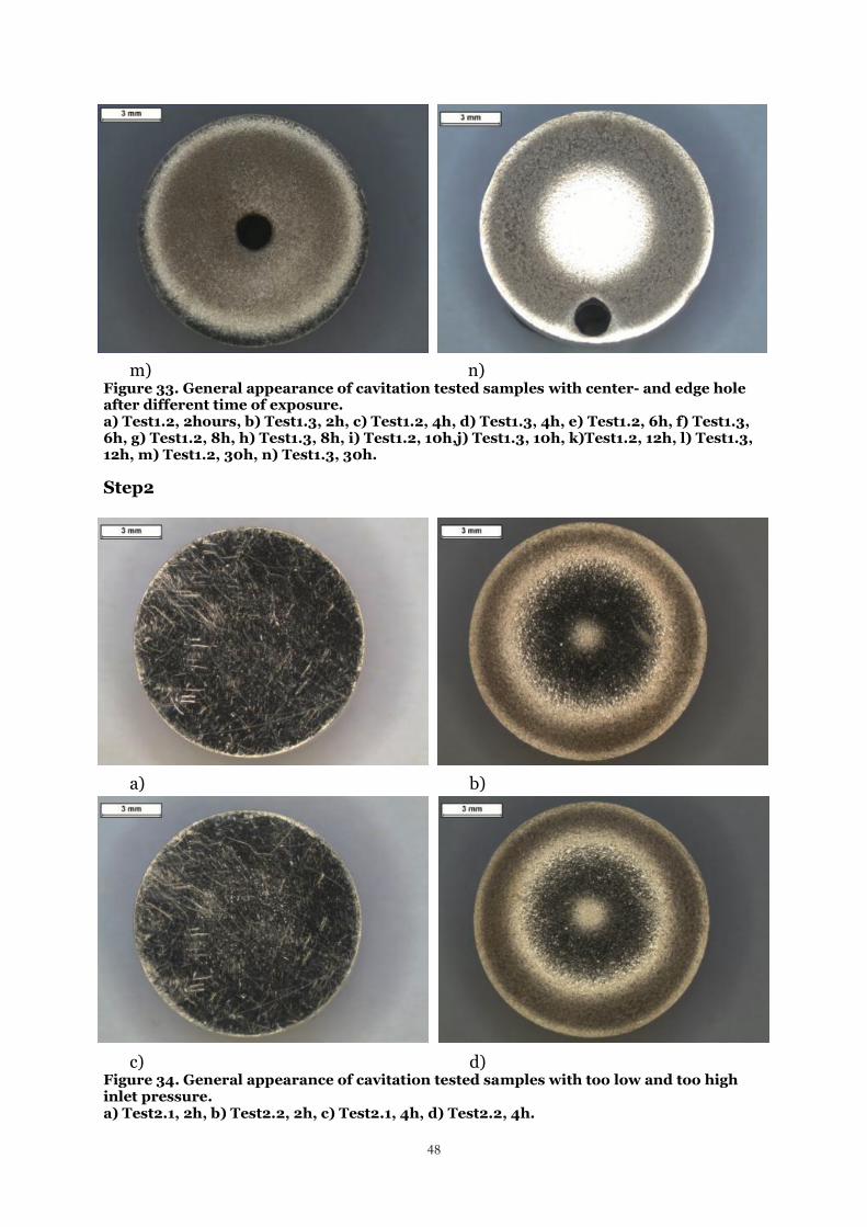
m) n) Figure 33. General appearance of cavitation tested samples with center- and edge hole after different time of exposure. a) Test1.2, 2hours, b) Test1.3, 2h, c) Test1.2, 4h, d) Test1.3, 4h, e) Test1.2, 6h, f) Test1.3, 6h, g) Test1.2, 8h, h) Test1.3, 8h, i) Test1.2, 10h,j) Test1.3, 10h, k)Test1.2, 12h, l) Test1.3, 12h, m) Test1.2, 30h, n) Test1.3, 30h.

Step2

a) b)

c) d) Figure 34. General appearance of cavitation tested samples with too low and too high inlet pressure. a) Test2.1, 2h, b) Test2.2, 2h, c) Test2.1, 4h, d) Test2.2, 4h.

49

a) b)

c) d)

e)

Figure 35. General appearance of cavitation tested sample with the higher cavitation number 0,0244. a) Test3.1, 2h, b) Test3.1, 4h, c) Test3.1, 8h, d) Test3.1, 12h, e) Test3.1, 30h.

50

APPENDIX III Figures from tests in chapter 5.2

In this appendix additional figure from chapter 5.2 is presented.

Test Pb

Figure 36. Average accumulated volume loss from the tested series of leaded tin bronze with deviations shown by error- bars.

a) b)

0,0000

0,5000

1,0000

1,5000

2,0000

2,5000

3,0000

3,5000

0 1 10

Vo

lum

e lo

ss [

mm

3 ]

Time [log(h)]

Leaded tin bronze

51

c) d)

e) f)

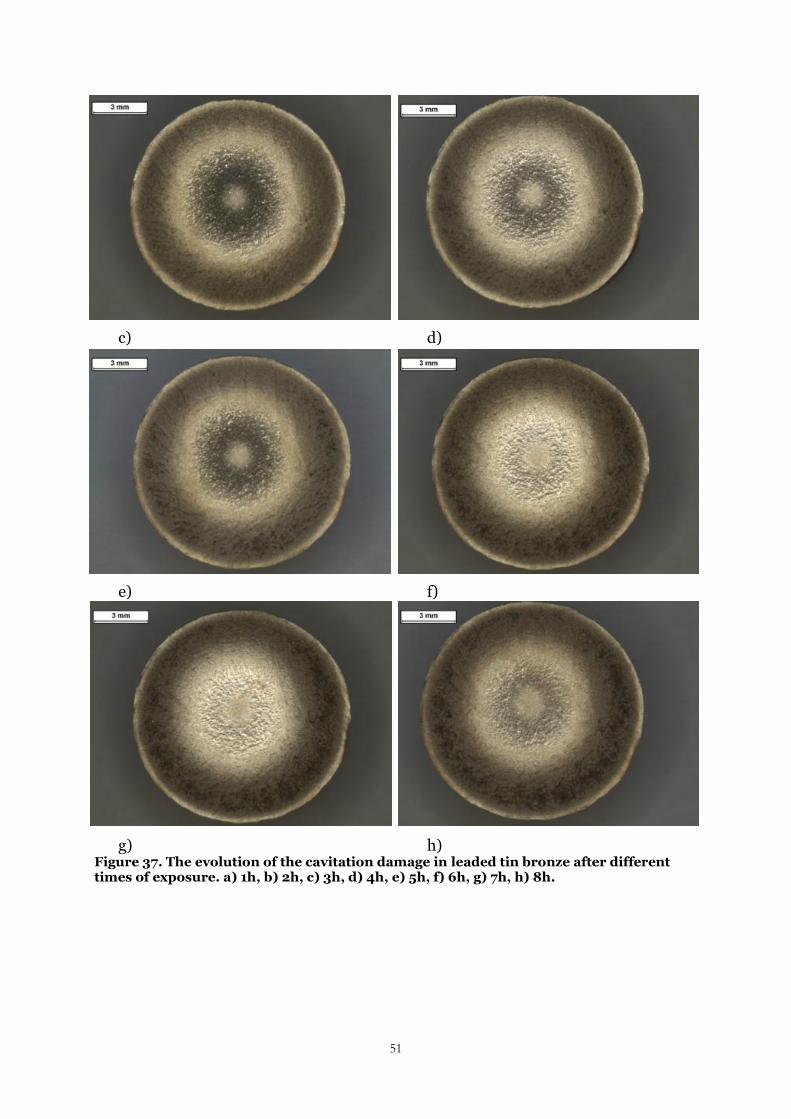
g) h) Figure 37. The evolution of the cavitation damage in leaded tin bronze after different times of exposure. a) 1h, b) 2h, c) 3h, d) 4h, e) 5h, f) 6h, g) 7h, h) 8h.

52

Test Sn

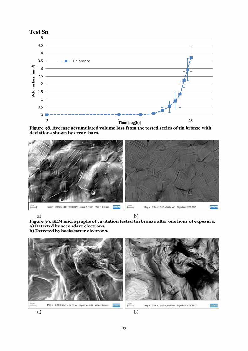
Figure 38. Average accumulated volume loss from the tested series of tin bronze with deviations shown by error- bars.

a) b) Figure 39. SEM micrographs of cavitation tested tin bronze after one hour of exposure. a) Detected by secondary electrons. b) Detected by backscatter electrons.

a) b)

0

0,5

1

1,5

2

2,5

3

3,5

4

4,5

5

0 1 10

Vo

lum

e lo

ss [

mm

3 ]

Time [log(h)]

Tin bronze

53

Figure 40. SEM micrographs showing cavitation tested samples of tin bronze after two hours of exposure. a) Detected by secondary electrons. b) Detected by backscatter electrons.

a) b)

c) d)

e) f)

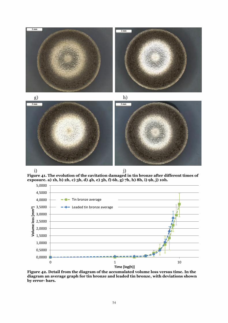
54

g) h)

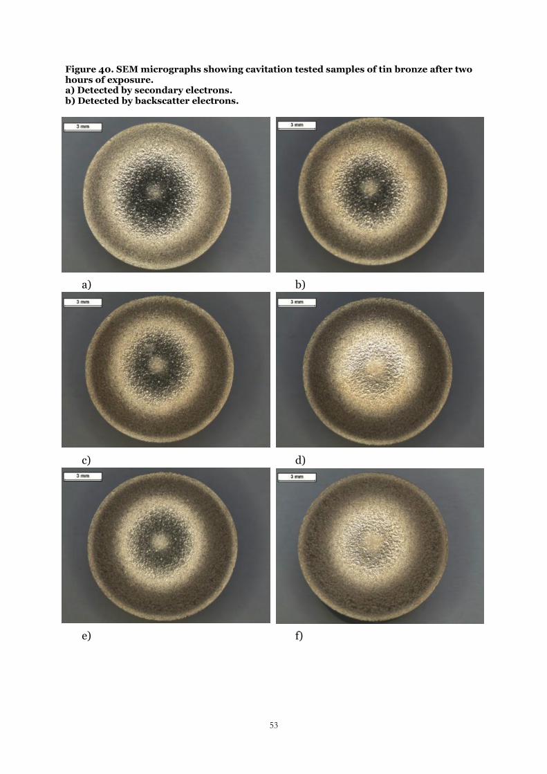
i) j) Figure 41. The evolution of the cavitation damaged in tin bronze after different times of exposure. a) 1h, b) 2h, c) 3h, d) 4h, e) 5h, f) 6h, g) 7h, h) 8h, i) 9h, j) 10h.

Figure 42. Detail from the diagram of the accumulated volume loss versus time. In the diagram an average graph for tin bronze and leaded tin bronze, with deviations shown by error- bars.

0,0000

0,5000

1,0000

1,5000

2,0000

2,5000

3,0000

3,5000

4,0000

4,5000

5,0000

0 1 10

Vo

lum

e lo

ss [

mm

3 ]

Time [log(h)]

Tin bronze average

Leaded tin bronze average

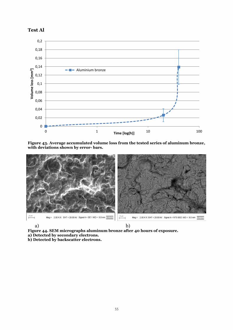
55

Test Al

Figure 43. Average accumulated volume loss from the tested series of aluminum bronze, with deviations shown by error- bars.

a) b) Figure 44. SEM micrographs aluminum bronze after 40 hours of exposure. a) Detected by secondary electrons. b) Detected by backscatter electrons.

0

0,02

0,04

0,06

0,08

0,1

0,12

0,14

0,16

0,18

0,2

0 1 10 100

Vo

lum

e lo

ss [

mm

3 ]

Time [log(h)]

Aluminium bronze

56