Defining ecologically or biologically significant … ecologically or biologically significant areas in the open oceans and deep seas: Analysis, tools, resources and illustrations

Defining ecologically or biologically significant areas in the

open oceans and deep seas:

Analysis, tools, resources and illustrations

A background document for the CBD expert workshop on scientific and technical guidance

on the use of biogeographic classification systems and identification of marine areas beyond

national jurisdiction in need of protection,

Ottawa, Canada

29 September – 2 October 2009

Authors: Jeff Ardron, Daniel Dunn, Colleen Corrigan, Kristina Gjerde, Patrick Halpin, Jake

Rice, Edward Vanden Berghe, Marjo Vierros

Illustrations edited by Daniel Dunn, with contributions from Jesse Cleary, Patrick N. Halpin,

Ei Fujioka, Ben Best, Jason Roberts, Andre Boustany, Jeff Ardron, Autumn-Lynn Harrison,

Ben Lascelles, Lincoln Fishpool, Piers Dunstan, Kristin Kaschner, Marjo Vierros, Sheila

McKenna, Arlo Hemphill, Edward Vanden Berghe, Malcolm Clark, Mireille Consalvey, Ashley

Rowden

ii

Table of Contents

Executive Summary ....................................................................................................................................... 1

Introduction .............................................................................................................................................. 3

A brief history of the Ecologically or Biologically Significant Areas (EBSA) criteria development

process .................................................................................................................................................. 4

Discussion of the EBSA criteria ..................................................................................................................... 5

Criterion 1: Uniqueness or rarity .............................................................................................................. 5

Definition (from CBD Decision IX/20 Annex 1) ..................................................................................... 5

Comments on the definition ................................................................................................................. 5

Comments on the application of this criterion ..................................................................................... 5

Methods ................................................................................................................................................ 6

Criterion 2: Special importance for life-history stages of species ............................................................ 7




Methods ................................................................................................................................................ 7

Criterion 3: Importance for threatened, endangered or declining species and/or habitats .................... 9




Methods ................................................................................................................................................ 9

Criterion 4: Vulnerability, fragility, sensitivity, or slow recovery ............................................................ 10

Definition (from CBD Decision IX/20 Annex 1) ................................................................................... 10

Comments on the definition ............................................................................................................... 10

iii

Comments on the application of this criterion ................................................................................... 10

Methods .............................................................................................................................................. 10

Criterion 5: Biological productivity ......................................................................................................... 11




Methods .............................................................................................................................................. 12

Criterion 6: Biological diversity ............................................................................................................... 13




Methods .............................................................................................................................................. 13

Criterion 7: Naturalness .......................................................................................................................... 14




Methods .............................................................................................................................................. 14

Sampling and data issues, including strategies for dealing with weak or incomplete data ................... 16

Types of data ....................................................................................................................................... 16

Data storage and retrieval systems: ................................................................................................... 17

Strategies for dealing with weak or incomplete data ......................................................................... 19

Annotated list of most important data sources .................................................................................. 20

Capacity building ..................................................................................................................................... 22

Future work ............................................................................................................................................. 23

1. Sharing information and progress .................................................................................................. 23

iv

2. Other outstanding work .................................................................................................................. 24

3. Consideration of EBSAs in the near future ..................................................................................... 24

Annex I ........................................................................................................................................................ 25

Additional Considerations for Practitioners................................................................................................ 25

1. Scale ............................................................................................................................................ 25

2. Relative importance / significance .............................................................................................. 27

3. Spatial and temporal variability .................................................................................................. 28

4. Precision, accuracy, and uncertainty .......................................................................................... 29

Literature cited in main text and Annex 1 .............................................................................................. 30

Comments Comments on this document are invited and may be provided at the Ottawa workshop and also directly

to Kristina M. Gjerde, IUCN High Seas Policy Advisor, at [email protected]. until 10 October.

Acknowledgements The authors of this document would like to gratefully acknowledge the support of the German Federal

Agency for Nature Conservation and the German Federal Ministry for the Environment, Nature

Conservation and Nuclear Safety, the Census of Marine Life, the Sloan Foundation, the Richard and

Rhoda Goldman Fund, the JM Kaplan Fund and the UK’s Department for Environment, Food and Rural

Affairs for this collaborative endeavour. We would also like to thank Dr. Jihyun Lee of the CBD

Secretariat for her guidance in the development of this document.

mailto:[email protected]

1

Executive Summary

The Conference of the Parties (COP) to the Convention on Biological Diversity (CBD) adopted in 2008

scientific criteria for identifying ecologically or biologically significant marine areas (EBSAs) in need of

protection. The application of these criteria will specifically focus on the open oceans and deep seas,

which encompass regions of the Earth that we have only started to explore. While much scientific

discovery lies ahead, available information and current and emerging methodologies already allow us to

begin identifying oceanic features that are likely of particular ecological or biological importance.

In order to facilitate this process, the CBD COP decided to convene an expert workshop to review and

synthesize progress on the identification of areas beyond national jurisdiction which meet the adopted

CBD scientific criteria. There are an increasing number of scientific techniques that could be used in

application of each of the seven criteria (Uniqueness or rarity; Special importance for life history of

species; Importance for threatened, endangered or declining species and/or habitats; Vulnerability,

fragility, sensitivity, slow recovery; Biological productivity; Biological diversity; and Naturalness). This

document provides a general overview of these techniques, and discusses key issues concerning the

strengths, challenges and limitations in the availability of data and scientific understanding we face at

this time.

This document reviews the description of each of the scientific criteria and comments on their potential

applications, discusses a variety of ways in which the scientific community understands these criteria,

and how they can be used as a foundation for informing future decisions regarding the marine

environment of the open oceans and deep seas. An important component of the document is a set of

practical illustrations (Annex 2) to increase our understanding of how the seven scientific criteria can be

applied. These provide a range of examples considering species, habitats and recurrent oceanographic

features using a variety of techniques ranging from field surveys, satellite tracking of tagged animals and

remote sensing, to sophisticated modelling and range prediction. These illustrations are not meant as

proposals for specific management measures, but are simply presented as examples of various scientific

methods and techniques relevant to each criterion.

Many types of data, including both physical and biological data, are needed to fully evaluate the

ecological or biological significance of a marine area. The document describes available data storage and

retrieval systems, and provides an annotated list of important, publicly-available data sources. Given the

paucity of data for deep seas and open oceans, it is important that all available data can be used to the

greatest extent possible to facilitate the eventual identification and evaluation of EBSAs. Making data

and information publicly available and easily accessible through relevant data archives and warehouses

will support further research and potential management applications.

Data sharing will also support the making of robust predictions for areas that remain relatively

unknown. In the absence of good broad scale survey data, limited high quality data can be used to

calibrate predictive modelling of the occurrence or abundance of a species or physical ecosystem

2

features. While predictive models are not a substitute for observations, if adequately validated, they can

make important contributions to evaluation of EBSAs.

Annex 1 of this document contains considerations for practitioners, which are more technical in nature.

The annex consolidates inputs from a variety of scientific and technical experts on overarching

considerations that practitioners may wish to take into account in applying the criteria. These

considerations include the scale of application of the criteria and accounting for relativity, variability,

and uncertainty. While the discussion is necessarily technical, this Annex provides practitioners with

valuable information about how to deal with fluid ocean systems that are often data-poor and show

variability on a range of spatial and temporal scales and across different levels of ecological complexity.

As the collective experience of CBD Parties in applying the scientific criteria grows, there is a need to

ensure that lessons learned are made widely and rapidly available to improve overall practices and to

facilitate international cooperation. In this regard, there would be great value in establishing a central

repository of EBSA-related information, including documentation of expert advisory processes (from

inputs to results), and any governance actions that may result from such processes. An important part of

this is providing for capacity building and transfer of experience to those who lack the immediate

scientific and technical capacity to apply the criteria.

3

Introduction The ecological and biological importance of the open oceans and deep seas have often been

underrepresented or misrepresented in discussions of global biodiversity and ecosystem function.

Contrary to some popular conceptions, the open oceans and deep seas are not uniform, barren and

relatively lifeless regions of our planet. Rather, these areas contain some of the most productive

ecosystems, unique habitats, and globally rare species yet discovered. From highly productive

seamounts to unique hydrothermal vent communities, to migratory pathways of endangered sea

turtles, the remote oceans support an enormous wealth of ecosystem productivity, specialized habitats

and individual species supporting both critical ecosystem functions and critical examples of our shared

biological heritage. The open oceans (pelagic) and deep seas (benthic) represent the largest biomes of

our biosphere in both surface area and volume. The dominance of the open oceans is a defining global

feature and the reason why Earth is viewed from space as the blue planet.

There are many historic and technical reasons why open ocean and deep sea ecosystems have been

relatively underrepresented for their biological and ecological significance to date. Open oceans and

deep sea areas are distant from human populations and are often inaccessible without significant

technological intervention. Centuries of navigation traditions have been replaced by other systems of

communication. However, the accumulated assembly of new technologies and new research findings

are now helping to “illuminate” the deep ocean areas of our planet and are providing a significantly

more detailed and comprehensive view of these regions and ecosystems. While much scientific

discovery lies ahead, the characteristics and locations of oceanic features that are of particular

importance, ecologically or biologically, are already emerging.

Because the open oceans and deep seas often fall outside of national jurisdictions, an international and

cooperative approach is fundamental to the characterization, location and eventual prioritization of

these important features for the protection of their critical roles in ecosystem processes. While much

information and many scientific methods can be extended from national surveys, international

cooperation will be critical in developing a common understanding in the application of scientific

criteria. The ongoing international processes convened by the Convention on Biological Diversity (CBD)

under the auspices of the United Nations Environment Program (UNEP) have been serving as a forum for

the development of initial criteria to define important areas in the open oceans and deep seas.

This document provides a general overview of current and emerging techniques that could be used in

the identification of ecologically or biologically significant areas (EBSAs), as well as highlighting key

issues concerning the strengths, challenges and limitations in the availability of data and scientific

understanding we face at this time. Annex 1 to this document presents a technical synopsis for

practitioners of some considerations with regard to application of scientific criteria, including issues

related to scale, relativity, variability, and uncertainty. Annex 2 provides contributed illustrations of

possible ways that ecologically and biologically significant areas (EBSAs --CBD Decision IX/20 Annex1)

could be identified in the open oceans and deep seas.

4

A brief history of the Ecologically or Biologically Significant Areas (EBSA)

criteria development process In 2007 a CBD expert workshop was convened in the Azores, Portugal, to develop, refine and

consolidate scientific and ecological criteria for the identification of marine areas in need of protection

and on biogeographical and other ecological classification systems. In 2008 the Conference of the

Parties (COP) to the Convention on Biological Diversity (CBD) adopted the scientific criteria (COP

Decision IX/20 paragraph 14) for identifying ecologically or biologically significant marine areas in need

of protection (COP Decision IX/20 Annex I) and guidance for designing representative networks of

marine protected areas in open ocean waters and deep sea habitats (COP Decision IX/20 Annex II). The

same decision also urged Parties and invited other Governments and relevant organizations to apply, as

appropriate, the Azores scientific criteria and guidance (paragraph 18). This background document

focuses on the scientific criteria in Annex I of the CBD Decision.

These criteria are based on seven general areas of consideration:

1. Uniqueness or rarity 2. Special importance for life history of species 3. Importance for threatened, endangered or declining species and/or habitats 4. Vulnerability, fragility, sensitivity, slow recovery 5. Biological productivity 6. Biological diversity 7. Naturalness

In addition, the COP Decision IX/20 (paragraph 19) included convening an expert workshop, where

scientific and technical experts were to provide scientific and technical guidance on the use and further

development of biogeographic classification systems, and guidance on the identification of areas beyond

national jurisdiction which meet the scientific criteria in Annex I of the decision.

The central task of the CBD expert workshop (Ottawa 2009) is to provide guidance on the identification

of areas beyond national jurisdiction which meet the scientific criteria in Annex 1 of decision IX/20. To

do so, the workshop will review and synthesize progress on the identification of areas beyond national

jurisdiction which meet the scientific criteria in Annex I to the present decision, and experience with the

use of the biogeographic classification system, building upon a compilation of existing sectoral, regional

and national efforts.

This background document and contributed illustrations have been developed to help inform the

current expert workshop process. The materials included in this document represent contributions from

a broad range of individuals and institutions with expertise in marine ecology, biogeography, mapping,

visualization and knowledge management. The intention of this compilation is to help inform general

discussion and provide illustrative examples of how EBSA criteria can be applied in the oceans, not to

suggest specific sites to be considered for designation of protective measures.

5

Discussion of the EBSA criteria In the following sections, a description of each of the EBSA criteria and comments on the potential

application of these criteria are presented. The purpose of this discussion is to present a variety of ways

in which the scientific community understands these criteria and how they can be used as a foundation

for informing future decisions regarding the marine environment of the open oceans and deep seas. This

overview is complemented by Annex 1 on Considerations for Practitioners that provides a more

technical discussion concerning general issues such as scale of application of the criteria, and issues

related to precision, accuracy and uncertainty and data availability, and Annex 2 with illustrations of

various ways the criteria can be applied to identify significant areas.

Criterion 1: Uniqueness or rarity

Definition (from CBD Decision IX/20 Annex 1)

Area contains either (i) unique (“the only one of its kind”), rare (occurs only in few locations) or endemic

species, populations or communities, and/or (ii) unique, rare or distinct, habitats or ecosystems; and/or

(iii) unique or unusual geomorphological or oceanographic features.

Comments on the definition

This criterion is established to identify unique or rare occurrences of species or habitats for

consideration. The uniqueness or rarity of a given feature may be determined at a variety of scales,

including the global, ocean basin, regional, or local scale. While ‘uniqueness’ by definition cannot be

judged on a relative scale (i.e. an object is either unique, or it isn’t), ‘rarity’ may be judged relative to

other species or habitats.

Comments on the application of this criterion

Rarity and Uniqueness are strongly influenced by the scale at which the policy and management

jurisdiction is functioning (the material for practitioners on Scale (Annex I) is relevant to the application

of this criterion). Global rarity should be taken into account when applying this criterion at regional or

local scales, such that a globally rare or unique property is identified as significant even if it is relatively

common within the specific region or locality for which the evaluation is conducted. However, a feature

that is depleted, rare or unique at the scale of a specific jurisdiction’s evaluation should also be

considered, even if the feature may be more common elsewhere.

In areas where biological information is scarce, physical data may provide the only basis for application

of this criterion. Areas that have unique substrates and bathymetries may be appropriate as EBSAs

based on this criterion, even without data on the biological communities present in the physically

unique sites. For example, in the eastern Australian margin survey using multibeam bathymetry to map

>25,000km2 of the seabed, only 31 km2 (0.12%) of seabed was comprised of hard substrata, while the

remaining seabed comprised bioturbated soft-sediment plains. In such a circumstance it is appropriate

6

to assume that the biotic community supported by rare physical geography (i.e. hard substrata in this

case) is also rare and should be considered as ecologically or biologically significant.

For most of the deep sea, there is an emerging consensus that many species are fairly rare, and thus

that “rarity is common.” If this is true, this part of the criterion for deep sea areas may pose some initial

difficulties. That said, some deep sea species are likely to be more rare than others.

Methods

Application of the Uniqueness & Rarity criterion may be based on biological, ecological and oceanographic information from peer reviewed literature, technical reports and data sets. As was done in the Sargasso Sea study (see Annex 2), areas containing similar features may be compared to assess the ways in which one area is different or unique. Uniqueness or rarity can also be based on similar comparisons of survey data.

It must be noted that this criterion poses particular challenges when applied in the deep sea due to the fact that much of these ocean regions have not been well studied. Given the limited sampling that has been done on deep-sea communities, applying this criterion beyond directly surveyed areas requires the creation of predictive models using appropriate survey data. Physical features such as rugosity, depth, and benthic complexity can be remotely sensed and are widely used in habitat modeling. Such variables have proven to be indicators of habitat for different species, and as such they are often used to classify benthic habitats and to quantify the availability of particular habitats and their obligate (directly associated) species. There are many techniques currently used to create such predictive models (see Predictive Modelling, Annex 1), and the validity and usefulness of the method has been repeatedly proven. However, these techniques tend to over-estimate the possible habitat for a given species or community and hence are prone to errors of commission, which could lead to the protection of areas where the predicted species do not actually exist, unless they are followed-up with in situ surveys. Building on these studies, it may be possible to reliably identify unique or rare combinations of such physical features where reliable biotic survey data are not yet available. Illustrations of how the criterion could be applied

Practical examples of how the uniqueness or rarity criterion could be applied can be found in Annex 2.

These illustrations relate to the Saya de Malha Banks in the Indian Ocean and to the Sargasso Sea in the

North Atlantic, and are based on a review of literature. It should be noted that these illustrations are

presented as examples of how the criterion could be applied, and are not meant as a proposal for

specific management measures.

7

Criterion 2: Special importance for life-history stages of species


Areas that are required for a population to survive and thrive.


This criterion is intended to identify specific areas that support critical life-history stages of individual

species. This is an inclusive definition which incorporates all life history stages of a species or population,

but which leaves open the question of how an area can be determined to be “required” for survival and

reproduction.


The application of this criterion will focus on the reliability and exclusivity of use of an area for a

particular life history function of one or more species. The “significance” of an area increases as either

factor (reliability over time, exclusivity relative to alternative areas) increases; i.e. “significance”

increases as a greater percentage of the species use an area more regularly (in time and space) for an

important life history function. It is also noted that sex, age and other biological variables can influence

where these important areas exist within a single species (i.e., females with nursing offspring vs. single

males), so caution should be taken when looking at this criterion across one species or population. See

Annex 2: “Areas of special importance for the Antipodean Albatross in the Tasman Sea” for an example

of how the significance of an area has been quantified based on this criterion.

Application of this criterion for deep sea species can be difficult because specialized sampling gears are

needed to sample early life stages of deep waters species such that they are without contamination

from other depths. Species identifications of immature life-history stages of deep-water species are also

poorly described in many areas, making it hard to identify areas of special significance at the species

level when dealing with immature stages of many deep-sea species.

Methods

The two EBSA criteria, Special importance for life history stages of species and Importance for threatened, endangered or declining species and/or habitats, are quite similar in nature, sharing the same examples listed in Annex I to Decision IX/20: “(i) breeding grounds, spawning areas, nursery areas, juvenile habitat or other areas important for life history stages of species; or (ii) habitats of migratory species (feeding, wintering or resting areas, breeding, moulting, migratory routes).” Due to this similarity, they will be considered together to aid understanding of the analytical techniques necessary to identify important areas related to a species or habitat.

The primary sources of data for application of these criteria are either survey data or satellite tracking data. Where coverage is adequate, survey data can be used directly to determine abundance and density of animals within a particular area. This type of data is extremely important if practitioners are interested in using the percentage of a population that exists in a particular location as a threshold (see Birdlife International’s implementation of ‘Important Bird Areas’ (Annex 2) as well as considerations in Annex I). In evaluating whether data are adequate for direct evaluation of the functional importance of

8

an area, consideration must be given to how well the data capture the likely degree of natural variation in a species’ distribution and behaviour. Areas of occupancy or performance of specific life-history activities may vary greatly from year to year, season to season or at an even shorter time scale. Consequently, the degree to which the available data are merely “snapshots” (i.e. representative of conditions at a single point in time) affects whether observed absences can be used as justification that an area is not used by a species, or observed presences can be used as justification that an area is necessary for that life history function. The less representative in space and time the available data are considered to be, the more likely it is that an evaluation should at least augment direct observational data with tested models. Where there are insufficient data or knowledge for direct estimates, models can be used to predict the likelihood of occurrence or abundance of a species from physical and biological oceanographic data.

Satellite tracking data offers more detailed information about a single organism’s movement and can be used to identify core use areas for individuals or aggregated to better understand the importance of areas to a population(s). The more consistent the data are from multiple tracked animals, the more valuable such data are for identifying core use areas for individuals or populations through home range analyses, predictive habitat models or resource selection models. Some general techniques that can be used on tracking data are listed below in order from the least complex and least data-intensive, to the most complex and most data-intensive methods:

Sinuosity Analysis (Bell 1991; Grémillet et al. 2004)

Fractal Analysis (Laidrea et al.. 2004)

First-Passage Time Analysis (FPT; Fauchald & Tveraa 2003)

Kernel Analyses ((Laver & Kelly, 2008)

Regression, Autocovariate and other Habitat Modelling (Guisan & Zimmermann 2000, Dormann et al. 2007)

State-Space Models (SSM) (Morales et al. 2004, Jonsen et al. 2005)

Illustrations of how the criterion could be applied

Practical examples of how the criterion for special importance for life-history stages of species could be

applied using some of these techniques and models can be found in Annex 2. The illustrations relate to

the northern elephant seals, Antipodean albatross in the Tasman Sea, and Pacific white sharks.

9

Criterion 3: Importance for threatened, endangered or declining species

and/or habitats


Area containing habitat for the survival and recovery of endangered, threatened, declining species or

area with significant assemblages of such species.


This criterion targets threatened, endangered or declining species and their habitats for consideration.

As in the above criterion, the linkage between the area of concern and the endangered species is one of

the relative factors in the application of this criterion. The greater the persistence of use of an area, and

the greater the number of individuals from a threatened population that use the area, the more

important the area must be considered. The definition of a “significant assemblage” is not made explicit

in the definition of the criterion.


In the deep seas, assessment of species against criteria for risk of extinction is still in early stages, and

the ecological requirements of most such species are poorly known. As studies to determine the

population trend of a species are long term, data intensive processes, the application of this criterion

must be based on pre-existing determinations of the population status of a given species. In particular,

use of the IUCN RedList (http://www.iucnredlist.org) is clearly fundamental to understanding to which

species this criterion applies. In data deficient situations, the listing for organisms with similar life

history traits should be used until further information on the status of the species is available.

Methods

See discussion under previous criterion, Importance for threatened, endangered or declining species

and/or habitats.


Practical examples of how the criterion of importance for threatened, endangered or declining species

and/or habitats could be applied using some of these methods can be found in Annex 2. The illustrations

relate to critically endangered Pacific leatherback turtles and juvenile Atlantic loggerhead turtles.

http://www.iucnredlist.org/

10

Criterion 4: Vulnerability, fragility, sensitivity, or slow recovery


Areas that contain a relatively high proportion of sensitive habitats, biotopes or species that are

functionally fragile (highly susceptible to degradation or depletion by human activity or by natural

events) or with slow recovery.


This EBSA criterion is focussed on the inherent sensitivity of species, or habitats, to disruption. The core

concept here is that species with low reproduction rates or habitats with slow potential recovery to

perturbation, for example, exhibit an inherently higher level of risk to impacts than other species or

habitats. This differs from other interpretations of vulnerability (e.g. FAO 2009) which also consider the

level of exposure a species or habitat has to human disturbance. For this reason, the terms fragility and

sensitivity may be more appropriate as a descriptor in the application of this criterion.


“Fragility” and recovery time can be quantified by examining the life history characteristics of a species

or the inherent properties of the ecosystem features themselves in the face of perturbations. In

general, species that are long-lived, have a later than average age-at-first-reproduction, and those that

produce few offspring are likely to be considered sensitive and require long time periods to recover

from perturbation. Structure forming organisms, or habitats that require geologic time periods to form,

are also likely to be slow to recover. Expert advice should be sought to explain the nature of the

ecosystem properties that are considered sensitive, vulnerable, fragile or slow to recover.

Ideally, maps of the potentially sensitive or vulnerable ecosystem features would be available. Lacking

adequate data for such mapping, it would still be possible to identify the areas where ecosystem

features that were sensitive, vulnerable, fragile or slow to recover were known or likely to occur, based

on modeling or extrapolation of expert knowledge from better known areas.

Methods

Information on which species or biomes qualify as vulnerable, fragile, sensitive or slow to recover should be based on peer-reviewed scientific literature to the extent possible. Regardless, the fragility of certain features to certain pressures (e.g. ice-dependent communities to the effects of climate change) can be taken as self-evident, unless data indicating the contrary are produced. In some cases, expert opinion can be used where vulnerabilities or sensitivities are only just beginning to enter the peer review process. As with previous criteria, this criterion can be informed by survey data and models by using physical features known to be associated with biotic features that are sensitive or slow to recover (see below). Application of models that extrapolate results of studies in one area to other areas of similar features will be particularly helpful for evaluating sensitivity or recovery rate. In cases of particularly sensitive benthic features such as deep-water corals, merely documenting presence of the feature using the best applicable method above may be sufficient to conclude that the area would be highly relevant to this criterion, without direct evidence of how sensitive or fragile that particular stand of coral was. Although

11

such inferences seem obvious for features such as corals, similar evaluations are not straightforward for some other features of marine communities, including communities composed of a range of co-existing life history strategies. In such applications models that predict the sensitivity or fragility of particular community types would be helpful.

Additionally, there are global datasets that depict or model human impact (e.g. Halpern et al. 2008, hydrocarbon exploration leases, shipping routes fishing, undersea cables, etc.) that could be overlaid with maps of fragile or sensitive habitats or species range maps to identify areas that may be under greater risk of damage or loss.


A practical example of how the criterion for vulnerability, fragility, sensitivity, or slow recovery could be

applied using predictive modeling of species distributions can be found in Annex 2. The illustration

relates to global habitat suitability for reef forming cold water corals.

Criterion 5: Biological productivity


Area containing species, populations or communities with comparatively higher natural biological

productivity.


This criterion is specified to identify regions in the open oceans which regularly exhibit high primary or

secondary productivity. These highly productive regions are here assumed to provide core ecosystem

services and are also generally assumed to support significant abundances of other higher trophic level

species. The phrase “comparatively higher” highlights the relative (rather than absolute) nature of this

criterion. How much “higher” is left open to interpretation and is discussed further in Annex I (see

relative importance / significance).


Productivity is not the same as abundance, but at least in some instances abundance could be used as a

surrogate for productivity. For this criterion, remote sensing data may be especially helpful, because

methods for quantifying primary productivity are well developed (see Annex 2: Biological Productivity).

Many of the issues discussed in the Practitioners Annex 1 on spatial and temporal variation are

particularly important in the application of this criterion, because centers of high primary and secondary

productivity are known to vary between years, seasonally, and on short time scales, but overall core

centres in space can be identified.

High productivity near the surface may not necessarily mean higher productivity near the seafloor, as

currents may transport animals and nutrients hundreds of kilometres before they settle to the bottom,

and thus such transport mechanisms should be considered. Studies of benthic communities have

12

struggled for decades to partition productivity from standing stock of biomass, and to relate patterns in

both to histories of human activities in specific areas. That very large literature base should help to

guide application of this criterion.

Some ecosystems in the deep sea, such as hydrothermal vents and cold seeps, are also areas of high

biological productivity through the conversion of specific chemicals into energy that directly supports

complex communities and often endemic species.

Methods

A variety of pre-processed biological productivity analyses are available online. As such, little analysis

needs to be performed in order to apply this criterion to specific areas. For example, global datasets are

available for Chlorophyll-a, primary productivity, and secondary productivity. Analytical techniques may

be required to identify the patterns of spatial gradients from areas of high productivity to areas of low

productivity, or such information may be found in peer-reviewed literature. Geographic Information

Systems (GIS) often include tools to identify various percentage thresholds in data sets, which can

contribute to evaluating how different parts of a large area score on this criterion.

The identification of oceanographic features related to higher levels of biological productivity is a more

difficult task that does require analysis of oceanographic datasets. Complex algorithms exist to identify

sea surface temperature fronts (e.g., Cayula & Cornillon, 1992) and warm- and cold-core eddies (e.g.,

Isern-Fontanet et al. 2003). Fortunately for managers and practitioners, some of these algorithms have

been implemented in a user-friendly tool package, Marine Geospatial Ecology Tools, which is freely

available online (http://code.env.duke.edu/projects/mget; Roberts et al., in review).


Practical examples of how the biological productivity criterion could be applied using satellite

observations and readily available tools to identify areas of 1) high phytoplankton production and 2)

areas of high dynamic activity as sea surface temperature fronts can be found in Annex 2.

http://code.env.duke.edu/projects/mget

13

Criterion 6: Biological diversity


Area contains comparatively higher diversity of ecosystems, habitats, communities, or species, or has

higher genetic diversity.


This criterion identifies areas of high relative taxonomic or habitat diversity. The question of measuring

biological diversity has generated a whole literature base of its own, with no single agreed-upon

definition of “diversity.” Hence, this criterion could be considered in a number of different ways.


Measures of diversity generally consider one or more of the following factors: 1) number of different

elements (species, communities, etc., also referred to as “richness”); 2) the relative abundance of the

elements (“evenness” and other related measures); and 3) how different or varied the elements are

when considered as a whole (e.g. taxonomic distinctness). In applying this EBSA criterion all three

factors could be taken into consideration.

When species survey data are lacking, habitat characteristics can provide indications of diversity. Owing

to the greater number of possible niches, habitats of higher complexity (heterogeneity) are believed to

also harbour higher species diversity. For benthic habitats this can be approximated by measuring

physical topographic complexity or rugosity (e.g., Ardron 2002, Dunn & Halpin 2009). For pelagic

habitats, this can be estimated by identifying convergences of differing water masses. Interactions of

differing water masses generally support higher biological diversity than the individual water masses,

and areas of high physical energy may also have relatively high biological diversity, consistent with the

diversity-disturbance relationship than has been established for many terrestrial systems. However,

because of the complexity of the concept of biological diversity, and the large variance around the often

statistically significant relationships between diversity and specific features of the physical environment,

application of this criterion will probably be most usefully conducted with biological data, rather than

relying on physical covariates of diversity.

Methods

Analytical techniques to measure of biodiversity have been a recurrent theme in ecology for many years.

A number of indices exist to examine this concept:

Berger-Parker Index (Berger & Parker 1970, May 1975)

Simpson’s Index (Simpson 1949)

Shannon-Wiener Index (Shannon 1948)

Pielou’s Evenness Index (Pielou 1969)

Hurlbert (ES50) Index (Hurlbert 1971)

Rank Abundance Curves (Foster & Dunston 2009)

14


Practical examples of how areas of higher biological diversity could be discerned using some of the

analytical techniques identified above can be found in Annex 2. These examples relate to global patterns

of species diversity using Hurlbert’s index; overlaps of hotspots of marine mammal biodiversity and

global seamount distributions using a species distribution model; and patterns of biodiversity richness

and evenness using rank abundance curves.

Criterion 7: Naturalness


Area with a comparatively higher degree of naturalness as a result of the lack of or low level of

human-induced disturbance or degradation.


This criterion measures the relative “naturalness” of open ocean areas compared to other

representative examples of the habitat type. This criterion is a relative measure, and it is not required

that an area be pristine in order for it to be identified as an EBSA. “Comparatively higher” highlights the

relative (rather than absolute) nature of this criterion. How much “higher” is left open to interpretation,

but presupposes that one has at least some information or indications on historic states of the

ecosystems in the region where the criterion is being applied.


The “natural” state of ecosystems in an area is often not known, even for many well-studies areas, but

inferences of this status can be gleaned from other areas. There is even less information on the

“natural” state of open ocean and deep sea ecosystems. In practice, application of this criterion will

probably consider the history of human activity in an area where EBSA evaluations are being conducted.

Areas where there is a documented or suspected history of human activities will be considered less

“natural” than areas where there has been little human activity. Application of the criterion will also

require taking account of what is known of the impacts of each human activity on specific ecosystem

features – such as bottom trawl impacts on benthic habitats, populations, and communities; or the

effects of shipping noise and ship strikes on wildlife aggregations and migrations, collisions, and so on.

Methods

Mapping and analysing the cumulative effects of human maritime activities is a new and emerging field

of research. Recent studies have paved the way for analyses of human impacts globally (Halpern et al.

2007, 2008a, 2008b), and regionally (Eastwood et al. 2007; Ban & Alder 2008; Tallis et al. 2008; Halpern

et al. 2009). Though methodologies are still developing, promising approaches stratify effects according

to their type (physical, chemical, biological, etc.), taking into consideration both intensity and effect-

distance of the given stressor on a given habitat type (Ban et al, in review).

15

In most studies to date, stressors are considered additive or incremental when impacts are repeated.

However, stressors can be synergistic or interactive when the combined effect is larger than the additive

effect of each stressor would predict (Folt et al. 1999; Cooper 2004; Vinebrooke et al. 2004). Stressors

can also be antagonistic, when the impact is less than expected (Folt et al. 1999; Vinebrooke et al. 2004).

Recent meta-analyses have shown that stressor interactions are additive, synergistic, and antagonistic

with little ability to predict which will occur when, and with roughly equal proportions (Crain et al. 2008;

Darling & Côté 2008).

Given the unpredictability of effects, in the absence of additional information, assuming an additive

mechanism is perhaps the best way forward, though it could in some cases underestimate effects.

Bearing in mind that naturalness is a relative measure, regardless of the analytical details, the mapping

of cumulative stressors should reveal overall patterns that would be useful to identify possibly (more)

natural areas of a given habitat type. Stressors can be mapped using a GIS and overlaid on habitat maps

to predict the ‘naturalness’ of an area.


A practical example of how the naturalness criterion could be applied can be found in Annex 2. This

combines a global set of predicted large seamount locations with historical catch data from seamount

fisheries and other anthropogenic impact to identify areas of low impact in the South East Atlantic.

16

Sampling and data issues, including strategies for dealing with weak or

incomplete data

Sampling the ocean requires sea-going or remote sensing technologies that are usually expensive and

operate under conditions of severe weather and, for deeper ecosystems, high pressure and distance-

communication challenges. There can be geo-political challenges to sampling as well. Researchers and

policy makers are acutely aware of the limited sampling of the open ocean and deep-sea, and that

southern hemisphere oceans generally are more poorly sampled than northern hemisphere oceans, and

low and high-latitude seas generally more poorly sampled than mid-latitude seas. Furthermore, the

sampling which has occurred is not always comparable, making global and sometimes regional analyses

difficult. In recognition of the lack of sampling, it is imperative to effectively utilize what information

exists and ensure that future research efforts are aligned. Towards this end, better sharing of data must

be encouraged.

Types of data

Systematic decision-making requires a solid foundation from which information and knowledge can be

extracted to inform choices among a set of options. In the case of evaluating the degree to which

specific areas are ecologically or biologically significant, specific

criteria (the “EBSA criteria”) have been adopted. Using readily

available data and objective criteria, it is possible to apply these

criteria and evaluate areas to determine their ecological or

biological significance. Physical and biological oceanographic data,

from both remotely sensed and in-situ sources form the base of

any evaluation processes. In addition, data sources such as species

occurrence, surveys and satellite tracking data can be used to

identify specific regions that may be of biological interest due to

rarity of species or ecotype or because the region is particularly

important to one or more at risk species. Such data are necessary

components of the indices used to assess the importance of an area relative to these criteria (e.g., the

calculation of Hurlbert’s Index based on species occurrence data or range maps to describe the

Biological Diversity criterion (Annex 2)). The data may be on species presences and/or abundances,

seabed and substrate features, physical and biological oceanography, and may be observed directly,

remotely sensed, or collected through systematic surveys or opportunistically.

Many different types of data are needed to fully evaluate the ecological or biological significance of a

marine area. Two categories of data can be classified in the following way:

1. Physical: Physical oceanographic data include data on both static bathymetric attributes and on

dynamic hydrographic attributes. Static bathymetric data (e.g. depth or rugosity) are

informative about the presence of features such as hydrothermal vents, deep-sea trenches,

17

seamounts, cold seeps and submarine canyons. Commonly available dynamic physical

hydrographic datasets include sea surface temperature and temperature at depth, various

measures of sea surface height (e.g. mean sea level anomalies), geostrophic current data, wind

and wave data, salinity, dissolved oxygen, and more complex derived products identifying

fronts, eddies and other oceanographic features.

2. Biological: Biological data include measures of productivity (e.g. Chlorophyll-a measurements,

or modelled estimates of primary or secondary production), biomass, carbon, as well as data

from direct species observation (observer data, survey data and satellite telemetry data) and

their derivatives (i.e., predictive habitat and range maps).

Although these data are fundamental to any systematic analysis of the marine environment, the time

and expense required to collect many of these data types (e.g. species observation data, deep-seabed

physical and biological data) greatly limit data availability. Furthermore, much data and information are

still stored in formats that are not easily accessible (e.g., museum specimens, or non-digitised

literature). Given the paucity of data that are available, it is imperative that existing data be used to the

greatest extent possible and made publicly available for reuse by other researchers, managers, and

policy makers. Data discoverability is a serious issue and systems are currently being developed to help

with the process of understanding where to find and how to use relevant data.

Data storage and retrieval systems:

There are three main examples of data storage and retrieval systems:

1. Metadata systems – Metadata systems assist in discovery, and help to determine the fitness of the data for the applications being undertaken (e.g., is the spatial resolution adequate? Does the extent cover the area of concern?) Metadata assist in broadening the basis of information available to decision-makers and their technical advisors. There are few privacy issues or Intellectual Property Right concerns with metadata, and thus they are usually freely available. However, the creation of metadata is generally seen as a chore by the researchers who have collected the data. Examples of metadata databases are the Global Change Master Directory of NASA (general environmental), OceanPortal of International Oceanographic Data and Information Exchange (IODE) of the Intergovernmental Oceanographic Commission (IOC; specific to marine environment), World Conservation Monitoring Centre (WCMC; specific to conservation).

2. Data archives – Data archives assist in data preservation. Data archives have all the detail of the original datasets, as the data are stored in a manner that mimics the data originator’s format as closely as possible. The major obstacle to data archives is convincing data generators (usually scientists) to contribute data to the archive. Many researchers view their data as proprietary and do not want to share them. Contribution of data to archives often also requires thorough metadata to be generated for the dataset, again raising the issue of the time required and the limited perceived benefit to the individual scientist of going through this process. Examples of data archives include the US National Oceanographic Data Center (NODC), and many other data centres of the IODE/IOC. These archives are usually supported by a data discovery tool/metadata catalogue.

18

3. Data warehouses – Data warehouses integrate data from other sources. The data stored in these warehouses are often of lesser detail than the original dataset, as data warehouses integrate data into one primary database that can only be as detailed as the least detailed dataset it incorporates. Data warehouses apply quality control standards and, when implemented properly, provide an audit trail (i.e., data can be traced back to data originator and any change is documented). Data warehouses face the same issues relating to data submission raised in the data archives section above. Examples of data warehouses include the World Ocean Database and World Ocean Atlas, products of the US NODC as World Data Center for Oceanography (indispensable for much oceanographic work). The Global Biodiversity Information Facility (GBIF) and the Ocean Biogeographic Information System (OBIS: http://iOBIS.org) are now emulating physical oceanographers and compiling species distribution records.

Although each type of data storage and retrieval system has its own niche, all three ‘systems’ have to

interlink. Metadata without access to data (through archives or warehouses) is informative, but of

limited value as the data cannot be repurposed without extra effort by the potential additional users.

Data warehouses are compilations, and so by definition are larger than the constituting individual

datasets. The aggregation of datasets into a database of sufficient size makes new types of analysis

possible. The greater geographic, temporal or taxonomic scope of the data warehouses allow for

stronger and larger scale patterns to be observed. However, it is often necessary to go to individual

datasets housed in data archives. Global databases are still relevant to the process, though, as they can

be used to seed local databases, and for quality control (e.g. check on species identifications by

comparison with known ranges).

Global databases also provide frameworks (e.g., standards, technology, networking) to facilitate further

integration, and provide input for the modelling of a species’ distribution – e.g. the use of environmental

maxima and minima to characterize habitat suitability on a finer scale. Models are not a substitute for

real observations, but will be necessary and important contributions to the evaluation of EBSAs if they

have been adequately ground-truthed and validated. They can be a buffer against faulty conclusions

caused by observer bias. For example, when survey data are not standardized by the amount of effort

employed, inaccuracies or biases can result from intensity or longevity of the effort and result in higher

numbers of species. In turn, these “rich areas” are an artefact of effort rather than a true estimate of

species presence. If the models perform consistently well in areas where independent knowledge is high

and their predictions can be tested rigorously, then they can be applied in situations where relevant

local data do not exist but decisions are necessary. Predictions from good models are better than

making a decision with little or no information whatsoever.

As part of the process of evaluating EBSAs in areas beyond national jurisdictions, Parties and relevant

organizations will need to support data archives and warehouses, provide data to them, and encourage

the process of data recovery (i.e. digitizing historical data). These can enable the making of robust

predictions based on sound models where data are sparse.

19

Strategies for dealing with weak or incomplete data

Predictive modelling

As indicated above, it is highly likely that practitioners will be faced with insufficient data to allow them

to directly evaluate the importance of an area based solely on that data itself. Under such

circumstances, the development of predictive models is a necessary step. Evaluation of any area of the

open ocean or deep sea is simply not currently possible without such models. In the absence of good

broad scale survey data, limited high quality data can be used to calibrate predictive models of the

occurrence or abundance of a species or physical ecosystem features. Such modelling requires reliable

data on the occurrence (presence-only, presence-absence, or abundance) of the ecosystem feature(s)

relevant to the EBSA evaluation and possible covariates (i.e., environmental variables) which are likely to

be widely available or readily measured in the areas of interest. Models linking the EBSA feature(s) to

these more easily measured variables can use a variety of methods to assess relationships (e.g.,

Generalized Linear or Additive Models, Bayesian networks, and “entropy” machine-learning analyses

(e.g., Maxent; Phillips et al. 2006)). Results of modelling approaches always have uncertainty about the

predicted likelihood or abundance of an ecosystem feature, but good modelling methods include the

uncertainty of the prediction as well as the most likely value.

Biogeographic classifications

Another possible way to address data limitations in specific areas is to apply experience from application

of the criteria in other areas with similar physical, chemical and biological characteristics. In addition to

input from experts, biogeographic classifications such as the Global Open Ocean and Deep Sea (GOODS)

may assist in identifying similar areas. Where there are places where no alternative areas are considered

similar enough to provide even coarse analogous information, this may itself be indicative of rarity or

uniqueness (see discussion of the Uniqueness and Rarity criterion and illustrations in Annex 2), and

further study should be encouraged to ground truth this assumption. Over time, knowledge of the open

ocean and deep seas will increase, as will experience with the use of these and possibly additional

criteria. Therefore any process for application of these criteria should include periodic reviews of

results.

Expert processes

Expert processes relying on people experienced with the use of data and their transformation into

information and knowledge can help to address data limitations, provided the processes are impartial,

as empirical as the information allows, and inclusive of the range of expertise available in the region.

Because the evaluations will almost inevitably require judgments by the experts, it is important that the

expert processes be transparent, and fully document the reasoning behind their evaluation. As Parties

begin to take the results of the expert evaluations and begin to design management measures to protect

EBSAs, certain types of evaluations may prove more (or less) useful in supporting policy and

management actions. To ensure these lessons are made widely and rapidly available to improve overall

practices, there would be great value to a central repository of EBSA-related actions, including

documentation of both expert advisory processes (from inputs to results), and governance actions with

the results of the expert processes.

20

Annotated list of important data sources

Government agencies typically maintain archives of environmental data, often the result of monitoring

activities. Each agency is responsible for their own type of data. Fisheries agencies are a prime source of

information for landing statistics of fish catch, and often also for monitoring data. Environmental

protection agencies are in charge of data on environmental quality. In many countries, a National

Oceanographic Data Centre (NODC) is providing facilities to archive many data types related to marine

sciences (e.g. NODC in the United States: http://www.nodc.noaa.gov. These NODCs work together in

the framework of the Intergovernmental Oceanographic Commission (http://ioc-unesco.org/) of

UNESCO. Specific examples of online resources for downloading oceanographic data are:

Bathymetry:

o SRTM30_Plus (see http://topex.ucsd.edu/WWW_html/srtm30_plus.html)

o ETOPO1 (see http://www.ngdc.noaa.gov/mgg/global/etopo1sources.html)

o GEBCO (see http://www.gebco.net/data_and_products/gridded_bathymetry_data/)

Sea Surface Temperature:

o AVHRR Pathfinder (see http://www.nodc.noaa.gov/SatelliteData/pathfinder4km/)

Ocean Color/Primary Productivity

o NASA OceanColor Chlorophyll (see http://oceancolor.gsfc.nasa.gov/)

o Vertically Generalized Production Model (VGPM; see

http://www.science.oregonstate.edu/ocean.productivity/)

Sea Surface Height1:

o AVISO sea surface height (SSH) data

o AVISO geostrophic current data

o AVISO significant wave height data

Sea Surface Wind:

o Quikscat (see http://podaac.jpl.nasa.gov/PRODUCTS/p109.html)

o AVISO Surface Wind data (http://www.aviso.oceanobs.com/en/data/products/wind-waves-

products/mswhmwind/processing-gridded-wind-wave-products/index.html)

Many science and fisheries advisory organisations are national, but some are regional and encompass

large areas of open ocean and deep sea, such as the International Council for the Exploration of the Sea

(ICES http://www.ices.dk/) in the Northern Atlantic and the North Pacific Marine Science Organization

(PICES http://www.pices.int/) in the Pacific. Also the UN Food and Agriculture Organization (FAO,

1 All available from AVISO at (http://www.aviso.oceanobs.com/en/data/products/sea-surface-height-

products/global/index.html)

http://www.nodc.noaa.gov/

http://ioc-unesco.org/

http://topex.ucsd.edu/WWW_html/srtm30_plus.html

http://www.ngdc.noaa.gov/mgg/global/etopo1sources.html

http://www.gebco.net/data_and_products/gridded_bathymetry_data/

http://www.nodc.noaa.gov/SatelliteData/pathfinder4km/

http://oceancolor.gsfc.nasa.gov/

http://www.science.oregonstate.edu/ocean.productivity/

http://comlmaps.org/how-to/layers-and-resources/oceanographic-data/aviso-sea-surface-height

http://podaac.jpl.nasa.gov/PRODUCTS/p109.html

http://www.ices.dk/

http://www.pices.int/

21

http://www.fao.org/) holds large amounts of data, but often aggregated to a level of detail that

becomes too coarse-grained to be used for purposes other than fisheries management.

Museums are traditionally the keepers of biodiversity information, storing physical specimens since

centuries. The progress in databases and communications via Internet has prompted many museums to

digitise specimen data, and make this information available through the World Wide Web (e.g.

Smithsonian, California Academy of Sciences, some European examples, Australia). The standards on

which both GBIF and OBIS were built were created with museum specimen data in mind.

A number of marine laboratories, such as the Sir Alistair Hardy Foundation for Oceanographic Studies

(SAHFOS, http://www.sahfos.ac.uk/) and the Scripps Institute of Oceanography

(http://www.sio.ucsd.edu/), have geospatially referenced collections of plant and animal specimens,

and related environmental data that span decades.

International scientific programmes such as the Joint Global Ocean Flux Study (JGOFS

http://ijgofs.whoi.edu/); Global Ocean Ecosystem Dynamics (GLOBEC http://www.globec.org/) and

InterRidge (http://www.interridge.org/) generate large datasets, which are typically available on line.

The Census of Marine Life (CoML http://www.coml.org/) deals specifically with marine biodiversity, on a

global scale; OBIS (http://iOBIS.org ) was created as its data integration component, and combines data

generated by CoML field projects with other sources.

Conservation organisations hold species information to support their conservation programmes, and

often work closely together with environmental managers. Examples include UNEP-WCMC species

databases (www.unep-wcmc.org/species/dbases/about.cfm), IUCN RedList

(http://www.iucnredlist.org/) and the Global Marine Species Assessment (GMSA,

http://sci.odu.edu/gmsa/). Increasingly, industries are holders of useful information based on direct

observations of species occurrences from their transport systems during business operations.

http://www.fao.org/

http://www.sahfos.ac.uk/

http://www.sio.ucsd.edu/

http://ijgofs.whoi.edu/

http://www.globec.org/

http://www.interridge.org/

http://www.coml.org/

http://iobis.org/

http://www.unep-wcmc.org/species/dbases/about.cfm


http://sci.odu.edu/gmsa/

22

Capacity building

Many developing countries, Small Island Developing States, and countries with economies in transition

may lack the scientific and technical capacity required for ready identification of EBSAs, particularly in

deep and open ocean areas. This lack of capacity may have to do with inadequate scientific data, or

access to equipment and technologies necessary to compile such data, relating to physical and biological

patterns, such as the distribution of species, habitats and ecosystems within national EEZs or beyond;

lack of knowledge and training relating to the best processes, methods and tools to use in identifying

EBSAs and moving from single sites to networks; limited hardware, software, or connectivity; and

inadequate human or financial resources to dedicate to the task. CBD decision IX/20 recognizes the

need to increase capacity and to exchange experiences, lessons learned and good practices related to

the identification of EBSAs.

There are a number of ways in which these capacity-related issues could be addressed. In the short to

medium-term, the following options exist:

Making information readily available regarding what data exists in the public domain and how

it can be accessed. International research programs, such as the Census of Marine Life, have

collected a great deal of scientific data from all regions of the world. These publicly available

data may fill some national information gaps in EBSA identification. Some of these are listed

above and more can be found in Annex II.

Implementing short training courses on the process of identifying EBSAs, including the use of

methods and tools. Such short courses are particularly useful for practitioners who are not able

to arrange for a lengthy leave of absence to pursue university studies.

Undertaking exchange visits between practitioners to learn first-hand the process of

identifying and designating EBSAs. These types of information visits can be arranged bilaterally,

or can be part of a broader learning network.

Sharing experiences and case studies through a dedicated web portal and/or a web-mapping

tool. The web portal and web mapping functions developed by Duke University and UNEP-

WCMC provide a platform for information sharing. In order for the information portal to

become widely used, it will need to be actively promoted at CBD and other

international/regional meetings, as well as through other means.

In the longer term, the following options might be explored:

Longer term degree programs and training courses to enhance scientific capacity, not only

relating to EBSAs, but to marine conservation biology, spatial ecology and other related

disciplines.

Development of a knowledge sharing network that provides professional expertise and advice

to governments wishing to identify EBSAs. This network would allow international experts to

23

work directly with practitioners to address issues specific to that country’s situation. A useful

model for a knowledge sharing network might be provided by the Cooperative Initiative on

Invasive Alien Species on Islands (“The Cooperative Islands Initiative” or CII), which provides

capacity building and technical support for on-the-ground projects relating to the management

and eradication of invasive species on islands (http://www.issg.org/cii/).

Future work

Sharing information and progress

The present document has provided an overview of some of the methods, analyses, tools and data

available for assessing areas that may meet the EBSA criteria. In addition, the document has shown a

number of illustrations regarding how such areas could be selected. While this is a good starting point,

work relating to the identification and eventual selection of EBSAs will continue in the long term and will

require the involvement of a large number of stakeholders, including scientists, governments,

international and non-governmental organizations, and industry. As improved data and methodologies

become available in the future, our capacity for evaluating and selecting EBSAs will improve.

Given the long-term nature of this work, there is a need to provide for support and coordination in the

process of identifying EBSAs. This support might include the sharing of experiences in regards to new

data, methods, decision-making tools, experiences and lessons learned. An important part of this

support would be in the form of capacity building activities, as described in the previous section.

Another vital component would allow scientists to share best available information, address technical

questions, and make information broadly available. As new potential EBSAs are identified, a central

register of proposed EBSAs would allow the scientific evaluation of such proposals to be undertaken in a

transparent and coordinated manner.

At a most basic level, coordination might be provided for through a common access point to EBSA-

related information. Information and experiences could be shared through the development of a

website portal on open oceans and deep seas. One such portal is already being tested by the Duke

University Marine Geospatial Laboratory, as part of their work on the Census of Marine Life project. This

portal aims to eventually provide for data and information exchange, collaborative processing and

outreach. The prototype portal will be on-line at http://openoceansdeepseas.org/.

Another linked component involves mapping habitat features, species information and proposed EBSAs

through an interactive web-mapping facility. UNEP-WCMC is currently developing a web-based map

viewer of marine areas beyond the limits of national jurisdiction, which would incorporate

geographically referenced data layers. In its initial form, the map viewer would contain web-based GIS

data for the presentation of static EBSA case studies. Later refinement of the map viewer could include

possible interactive capacity, allowing the user to perform basic analyses with available data layers.

http://www.issg.org/cii/

https://owa.ias.unu.edu/exchweb/bin/redir.asp?URL=http://openoceansdeepseas.org/

24

Together, these two linked websites would provide for the sharing of data, methodologies and

experiences relating to deep and open oceans, as well as the capacity to map proposed EBSAs and make

available the GIS files. They would also provide for scientific and technical collaboration, as well as

capacity building, with the aim to ensure that policymakers will be able to access best available scientific

information for the management of remote and shared ocean areas.

Other outstanding work

Most of the examples presented in this document illustrate the application of single criterion to help

identify an EBSA. However, some areas could meet multiple EBSA criteria. For example, some

seamounts could be considered ecologically or biologically significant because they are of special

importance to life-history stages of species; un-fished seamounts may meet naturalness criterion; and

some seamounts have high productivity and uniqueness values. Hydrothermal vents may also meet

multiple EBSA criteria. An area might be designated for any one of these criteria or for meeting multiple

criteria. Using multiple criteria becomes particularly important once the process moves from identifying

individual EBSAs to networks. Once this stage is reached, there is a need to develop further guidance for

considering multiple EBSA layers as members of possible networks. In this regard, annexes II and III of

CBD decision XI/20 provide a basis on developing representative networks of marine protected areas.

However, as this document elaborates upon IX/20 Annex 1, further guidance will likely also be required

for Annexes 2 and 3, including the development of illustrative examples.

Consideration of EBSAs in the near future

While this document has been developed for use in the CBD Expert workshop in Ottawa, the scientific

work to help identify areas that may meet the EBSA criteria will continue well beyond 2009. Proposed

work includes capacity building, possibly in the form of future regional workshops, as well as bringing

together regional oceans and fisheries management agencies.

A number of international meetings during the coming years will be relevant to the EBSA work detailed

in this document, and may provide further direction for this work. These include the following:

January 2010: the Ad Hoc Open-ended Informal Working Group to study issues relating to the conservation and sustainable use of marine biological diversity beyond areas of national jurisdiction (New York).

3-7 May 2010: The Global Conference on Oceans, Coasts and Islands (Paris)

13-21 May 2010: CBD SBSTTA-14 (Nairobi, Kenya)

4-7 October 2010: Launch of the Census of Marine Life results

18-29 October 2010: CBD COP-10 (Nagoya, Japan)

2013: Marine mammal protected areas meeting with France hosting

25

Annex I

Additional Considerations for Practitioners

In order to identify additional considerations in application of the EBSA criteria, we requested input

from a variety of scientific and technical experts. These experts identified a common set of overarching

considerations that practitioners may wish to take into account in applying the criteria. Many of these

considerations arose from the fact that research—and thus knowledge -- of the open oceans and deep

seas is for the most part still in its infancy; data are few and sparse, and understanding of the underlying

ecosystem drivers and emergent processes is incomplete. Application of, and extrapolation from, the

existing information would therefore benefit from addressing, inter alia:

1. issues related to scale of application of each criterion;

2. evaluation of the relative importance / significance of an area for a given criterion;

3. accounting for spatial and temporal variability; and

4. precision, accuracy, and uncertainty;

This Annex provides guidance for practitioners for addressing each of these considerations, to aid in

consistent and objective application of the criteria by appropriate expert groups where information is

available to commence such work.

Scale Scale is a major concern in ecological applications (Levin 1992, Scheiner et al 2000). In this document it

is used broadly, to include the scale of patterns in space and time, shown by data about either structural

(criteria like fragility or uniqueness) or functional (criteria like special importance to life history stages)

ecosystem properties. Scale generally refers to the extent of the property being measured relative to

the unit of measurement, or “grain” (Schneider 2001). It reflects the amount of ecologically meaningful

detail available for any given analysis. It is influenced by both the accuracy and particularly the

precision, of sampling relative to the natural variability of the property being sampled. With regard to

application of the EBSA criteria, scale is relevant from both the ecological perspective and from the

implementation perspective.

From the ecological perspective, systems generally show characteristic variability on a range of spatial

and temporal scales and across different levels of ecological complexity (Levin 1992). At the species

level, an appropriate scale of study for one life history stage (e.g. larval) may be inappropriate for

another (e.g. juvenile). Consequently application of the criterion regarding importance to life history

stages of a species could require considering several different scales to capture the requirements of the

species. For such reasons there is no one right or correct scale for application of any of the criteria. This

is not a shortcoming of the EBSA criteria per se, but rather a general issue when studying ecological

systems (Thrush et al 1997). However, in applying the criteria it is often necessary to determine how

26

results can be translated from one scale to another, guided by the linkages among elements in the

system. When applying criteria of biological diversity and productivity, experience from terrestrial

ecology can sometimes provide guidance on making such translations among scales (e.g. the scaling up

of quadrat-plot results using species-area curves to predict regional species richness –Stohlgren et al

1997), including lessons about the risk of becoming lost in a myriad of arcane considerations (Scheiner

et al 2000). In general, for any of the criteria, if specific questions can be posed, appropriate scales are

usually fairly self-evident, such as the range of an individual, the distribution of a species, or the

persistence of an upwelling event.

Modern GIS technology allows users to work a multiple scales and often zoom in and out depending

upon what is of interest. This may result in GIS products that are not matched to any particular

intended scale, or vary in scale across a series of related products. Likewise, the results of modelling

(such as predictive habitat or biogeographic classifications) are not actually of uniform scale, with some

places reflecting better input data and confidence (less uncertainty) than others. Users who receive the

analysis or modeling products without explanation about the quality of information in space or time can

choose among unsatisfactory alternatives. For example, they might assume all the results are only as

good as their weakest components, thus sacrificing greater accuracy and precision in identifying EBSAs

and limiting their prioritization to the better known areas. Alternatively they may erroneously use all

the results as if they reflect as much information as the best cases, and overestimate the importance of

certain areas without accounting for the uncertainty in the model prediction.

Good practice for addressing scale in the application of EBSA criteria will require the creation of indices

of confidence such as estimated confidence layers to accompany analysis and modelling results. By

“confidence,” in this context we mean how certain one can be that the results reflect the true situation,

taking into account the many uncertainties associated with sound scientific analyses; that is, for a good

scientist, very little is 100% certain, but some things are more certain than others. Although it is very

difficult to take all uncertainties into account, practitioners should take account of as many factors as

possible, particularly the more readily available factors such as sampling design and density,

measurement accuracy, and so forth. Such factors are especially relevant if input GIS layers or data

series were aggregated or appended together from various disparate datasets of varying scales.

Estimated confidence layers in GIS analyses allows for better informed decisions and is highly

recommended when dealing with maps and data of varying scales. Even though methods for producing

such confidence layers are still evolving, decisions regarding the identification of EBSAs will be more

likely to succeed when estimated confidence is taken into account.

Even if an absolute value of uncertainty cannot be estimated, it is usually possible to estimate relative

confidence; i.e. Area A is considered to have more uncertainty than Area B. Simple relative confidence

scores (e.g. 1=lower; 2=moderate; 3=higher) for each input layer can go a long way towards producing

an overall relative confidence layer that is helpful for planning. Even qualitative guidance on the varying

scale (and quality) of the information, can guide the varying scale of decision-making from place to

place. Practitioners may prefer to focus their efforts on better understood areas rather than highly

uncertain ones, and/or to have some areas given larger buffers than others, in order to maintain a

consistent degree of risk aversion in face of varying levels of uncertainty.

27

Relative importance / significance All of the EBSA criteria (except for “Uniqueness”) are relative measures; i.e., they comparatively order

places that are more “significant” than surrounding areas based on the ecological or biological role

played by the area within the larger region where an evaluation of EBSAs is occurring. The properties of

marine ecosystems vary widely from region to region, so global absolute thresholds (i.e. measurement

‘X’ must exceed ‘a’ units) are not appropriate. Instead, the evaluation process must sort out the relative

importance of specific features or places in a given ecological region on each of the criteria. In the best

cases the ecological knowledge of the area can be used to establish and justify a particular threshold

value above which any area would be an EBSA on the given criterion. This is the ideal approach, but also

the most demanding of both data and ecological knowledge of an area.

Often there may be enough information to map the pattern of how a biological feature varies with

regard to a single variable, such as abundance, across an area. In these cases the patterns in the

available data may help inform how possible “significance” varies with the “abundance” (or other

attribute) of a feature. With comprehensive quantitative data, two general approaches can be used for

investigation of such patterns:

1. Identify natural break point(s) in the

data: The underlying assumption of this

approach is that with some types of

data exceptional features will naturally

stand out from all others. This approach

works well with data that have multiple

modes or clusters, such as infrequent

dense concentrations of features that

usually are thinly distributed. Plots of

frequency histogram (fig. 1) will bring

out this nature of the data when it is

present. Analytical methods applied to

such data can use the cumulative frequency distribution rather than the histograms, although

both methods of presentation display the same patterns in the data. “Steps” that appear in the

cumulative frequency distribution show how the data are clustered into groups that are similar

on the feature of interest. Many statistical techniques can be applied to make steps appear

larger or smaller, and to isolate the steps (places) at the high and low end of the distribution.

When applying these techniques, however, it is necessary to take care to avoid circularity and

confirmatory bias of making differences in the data look larger than they really are. Ecological

knowledge is still necessary to interpret the ecological or biological “significance” of the various

steps, and (when one is needed) justify a threshold value – that is, the value above (or below)

which areas are considered significant. If such knowledge is very weak, arbitrary choices can be

made about the use of a threshold value, but it is often sufficient to provide the numerical

rankings of sites as increasing in “significance” and highlight where the steps in the distribution

Figure 1. An example of a histogram showing two clusters of values

and the optimal threshold to differentiate between those clusters.

28

are, as input to the dialogue on how the degree of ecological or biological significance varies

among areas.

2. Select a cut-off based on standard deviations: If the data about the occurrence of the ecological

feature of interest are smooth and continuous, then analyses of their frequency distribution will

not reveal any discontinuities or steps. In such cases the sites at the high (or low for the “rarity”

criterion) end of the smooth distribution are more significant that ones closer to the centre.

There is a long statistical history of considering cases more than two standard deviations from

the mean to be “significant”, and such an arbitrary rule can be applied to identify a threshold

above or below which sites might be considered significant. However, it is important to note

that in this statistical convention, “significance” has traditionally had a different meaning from

that of 'biologically or ecologically significant.' The assumption that a feature that is statistically

unusual (“significant”) in its class is also biologically significant may or may not be true, though it

does suggest further investigation is warranted. In many circumstances data may need to be

transformed to better approximate a normal distribution before this method can be applied.

Spatial and temporal variability It is important to recognize that most aspects of the marine environment are highly dynamic. Thus,

when evaluating the ecological or biological significance of an area based on a particular criterion, the

spatial and temporal variability of a feature (e.g. a sea surface temperature front) or an organism’s

behaviour (e.g. migration routes) must be taken into account. For many criteria, some places will have

substantial variation in how they would be evaluated from year to year, season to season, or on even

shorter time periods. The science advice identifying the likely EBSA and suggesting appropriate

boundaries should include as much information as possible about the magnitude and time-scale of these

variations. How variability is incorporated into evaluations of an area is largely dependent on the type

of data being analyzed. When looking at oceanographic features (e.g., sea surface temperature fronts,

eddies, or upwelling events) practitioners can use threshold values to differentiate ‘persistent’ features

from temporary features using climatologies (i.e., average values over extended time periods). One

good example of this is the aggregation of daily sea surface temperature front data into a climatology

representing the likelihood that a front will exist in a given area (see Annex II: “Sea Surface Temperature

Fronts”). Such a dataset could then have threshold values applied to it to delineate important areas of

higher frontal activity.

It is equally important to examine spatial and temporal (spatio-temporal) variability in survey or tracking

data. Although it is tempting to aggregate data from different surveys or tracked animals together to

better understand population level processes, it is important to first consider how the data overlap in

time and space. For instance, tracking data from animals tracked in the fall may present very different

patterns of area utilization than those same animals tracked in the spring. To ensure that all areas

relevant to an organism’s life history are taken into account, temporal variations in these data should be

understood and incorporated into evaluations of an area’s importance. Generally, good data over a

number of years are necessary to meet this objective. For further discussion and examples of how to

incorporate spatio-temporal variability in survey and tracking data see Annex II.

29

Finally, it is necessary to consider variability induced by climate change and other global processes

(Fuller et al. 2008). These can affect oceanographic processes, and thereby species ranges, migration

patterns, and resource availability. As such, it is important to understand if there are temporal trends in

the data used to evaluate an area.

Precision, accuracy, and uncertainty Discussions of scale and spatial/temporal variability inevitably lead to discussions of precision, accuracy,

and uncertainty. These three properties of data are inter-related but not interchangeable. Evaluations

of the ecological or biological importance of an area require that practitioners accommodate the

uncertainty in the available information, which in turn requires understanding the factors that

contribute to the uncertainty. Uncertainty may enter evaluations of an area through several means, but

most commonly it is due to the use of predictive models, or through factors inherent in the sampling

method used (e.g., uncertainty in locational data recorded by tags used to track animals). For many

marine features it is difficult to take exact measurements, regardless of the precision of the scale of

measurement. Benthic sampling gears do not necessarily capture every individual in the location being

sampled; towed nets do not always cover exactly the distance that is recorded as “distance towed”.

Such measurement error contributes to uncertainty in the data as well. There is a large body of

scientific literature on survey, sampling, and experimental design which addresses how to deal with

potential bias and variance in research and surveys, and this literature should be consulted for guidance

on a case by case basis. Large sample sizes of repeated measurements can go far in addressing

measurement uncertainty, for example.

Uncertainty contributes to two types of possible errors in evaluating data relative to the EBSA criteria;

“misses” – when it is erroneously concluded that an area does not meet a criterion when in reality it

does, and “false positives”, when it is erroneously concluded that an area does meet one of the criteria,

when in reality it does not. Misses are likely when data are incomplete and/or sampling coverage at the

wrong scale (generally too coarse), so features are present in an area (or ecological functions served)

but they simply are not recorded in the available data. False positives also reflect incomplete

knowledge of an area, such that limited sample data are treated as typical, and a model is built around

them predicting a broader distribution of a feature than actually exists. Without groundtruthing, this can

lead to the protection of sites that do not actually have the desired feature. Both types of errors

decrease as ecological knowledge increases and sampling becomes more complete. With high

uncertainty in data and information, the precautionary approach would support a relatively higher

tolerance for false positives than misses. Thus, failure to find evidence of an EBSA in incomplete data

sets should not be taken as strong evidence that the area has no special requirements for conservation.

30

Literature cited in main text and Annex 1

Alpine, J. E., and Hobday, A.J. 2007. Area requirements and pelagic protected areas: is size an

impediment to implementation? Marine and Freshwater Research 58(6): 558–569.

Ardron, J.A., 2002. A Recipe for Determining Benthic Complexity: An Indicator of Species Richness. In,

Marine Geography: GIS for the Oceans and Seas (ch. 23, pp 196-175), Joe Breman (ed.). Redlands, CA,

USA: ESRI Press.

Ban N. & Alder J. (2008). How wild is the ocean? Assessing the intensity of anthropogenic marine

activities in British Columbia, Canada

Ban, N.C., Alidina, H.M., Ardron, J.A. In review. Cumulative impact mapping: advances, relevance to

marine conservation strategies.

Bell W.J. 1991. Searching behaviour : The behavioural ecology of finding resources. Chapman & Hall

Berger, W H; F L Parker (1970) Diversity of planktonic Foramenifera in deep sea sediments. Science

168:1345-1347.

Cayula, J.-F. and P. Cornillon (1992) Edge detection algorithm for SST images. Journal of Atmospheric

and Oceanic Technology 9: 67-80

Cooper L.M. (2004). Guidelines for cumulative effects assessment in SEA of plans. In: EPMG Occasional

Paper 04/LMC/CEA. Imperial College of London London, pp. 1-50.

Crain C.M., Kroeker K. & Halpern B.S. (2008). Interactive and cumulative effects of multiple human

stressors in marine systems. Ecol Lett, 11, 1304-1315.

Darling E.S. & Côté I.M. (2008). Quantifying the evidence for ecological synergies. Ecol Lett, 11, 1278-

1286.Eastwood P.D., Mills C.M., Aldridge J.N., Houghton C.A. & Rogers S.I. (2007). Human activities in UK

offshore waters: an assessment of direct, physical pressure on the seabed. ICES Journal of Marine

Science: Journal du Conseil, 64, 453.

Dormann CF, McPherson JM, Araújo MB, Bivand R, Bolliger J, Carl G, Davies RG, Hirzel A, Jetz W, Kissling

WD, Kühn I, Ohlemüller R, Peres-Neto PR, Reineking B, Schröder B, Schurr FM, Wilson R. (2007) Methods

to account for spatial autocorrelation in the analysis of species distributional data: a review. Ecography

30(5): 609-28.

Dunn, D.C., P.N. Halpin. (2009) Rugosity-based regional modeling of hard-bottom habitat. Marine

Ecology Progress Series 377:1–11.

Eastwood, P. D., Mills, C. M., Aldridge, J. N., Houghton, C. A., and Rogers, S. I. (2007) Human activities in

UK offshore waters: an assessment of direct, physical pressure on the seabed. ICES Journal of Marine

Science, 64: 453–463.

31

Fauchald, P. & Tveraa, T. 2003. Using first-passage time in the analysis of area-restricted search and

habitat selection. Ecology. 84 (2): 282-288FAO. 2009. International guidelines for the management of

deep-sea fisheries in the high seas. Food and Agriculture Organization of the United Nations, Rome.

Folt C.L., Chen C.Y., Moore M.V. & Burnaford J. (1999). Synergism and antagonism among multiple

stressors. Limnol Oceanogr, 44, 864-877.

Foster, S.D. and P.K. Dunstan (2009) The Analysis of Biodiversity Using Rank Abundance Distributions.

Biometrics. Available early online May, 2009. DOI: 10.1111/j.1541-0420.2009.01263.x

Fuller, T., Morton, D.P., Sarkar, S. 2008. Incorporating uncertainty about species’ potential distributions

under climate change into the selection of conservation areas with a case study from the Arctic Coastal

Plain of Alaska. Biological Conservation 141: 1547-1559.

Game, E.T, McDOnald-Madden, E., Puotinen, M.L., Possingham, H.P. 2008. Should we protect the strong

or the weak? Risk Resilience, and the selection of marine protected areas. Conservation Biology, 22(6):

1619–1629.

Game, E.T., Watts, M.E., Wooldridge, S., Possingham, H.P. 2008. Planning for persistence in marine

reserves: a question of catastrophic importance. Ecological Applications, 18(3): 670–680.Schneider, D.C.

2001. The Rise of the Concept of Scale in Ecology. BioScience, 51(7): 545-553.

Grémillet, D., Dell’Omo, G., Ryan, P.G., Peters, G., Ropert-Coudert, Y. & Weeks, S. 2004. Offshore

diplomacy, or how seabirds mitigate intraspecific competition : a case study based on GPS tracking of

cape gannets from neighbouring breeding sites. Marine Ecology Progress Series 268: 265-279

Guisan, A. and Zimmermann, N. E. 2000. Predictive habitat distribution models in ecology. Ecological

Modelling, 135: 147-186.

Halpern B.S., Kappel C.V., Selkoe K.A., Micheli F., Ebert C., Kontgis C., Crain C.M., Martone R., Shearer C.

& Teck S.J. (2009). Mapping cumulative human impacts to California Current marine ecosystems.

Conservation Letters.

Halpern B.S., McLeod K.L., Rosenberg A.A. & Crowder L.B. (2008a). Managing for cumulative impacts in

ecosystem-based management through ocean zoning. Ocean & Coastal Management, 51, 203-211.

Halpern B.S., Selkoe K.A., Micheli F. & Kappel C.V. (2007). Evaluating and Ranking the Vulnerability of

Global Marine Ecosystems to Anthropogenic Threats. Conserv Biol, 21, 1301-1315.

Halpern B.S., Walbridge S., Selkoe K.A., Kappel C.V., Micheli F., D'Agrosa C., Bruno J.F., Casey K.S., Ebert

C., Fox H.E., Fujita R., Heinemann D., Lenihan H.S., Madin E.M.P., Perry M.T., Selig E.R., Spalding M.,

Steneck R. & Watson R. (2008b). A Global Map of Human Impact on Marine Ecosystems. Science %R

10.1126/science.1149345, 319, 948-952.

Hasson F, Keeney S., McKenna H. 2000. Research guidelines for the Delphi survey technique. Journal of

Advanced Nursing 32: 1008-1015.

32

Hurlbert, S.H. (1971) The non-concept of species diversity: a critique and alternative parameters.

Ecology 52, 577–586.

ICES (2009) Report of the ICES‐NAFO Working Group on Deep‐water Ecology (WGDEC), 9–13 March

2009, ICES CM 2009\ACOM:23. 94 pp.

Isern-Fontanet, J., E. García-Ladona, and J. Font. 2003: Identification of Marine Eddies from Altimetric

Maps. J. Atmos. Oceanic Technol., 20, 772–778.

Jonsen, I.D., Flemming, J.M. & Myers, R.A. 2005. Robust state-space modelling of animal movement

data. Ecology. 86 (11): 2874-2880

Laidre, K.L., Heide-Jorgensen, M.P., Logsdon, M.L., Hobbs, R.C., Dietz, R. & VanBlaricom, G.R. 2004.

Fractal analysis of narwhal space use patterns. Zoology. 107: 3-11.

Laver, P. N. and Kelly, M. J. 2008. A Critical Review of Home Range Studies. Journal of Wildlife

Management, 72: 290-298.

Levin, S.A. (1992) The Problem of Pattern and Scale in Ecology. Adapted from the Robert H. MacArthur

Award Lecture, presented Aug. 1989, Toronto, Ontario, Canada. Ecology, 73(6): 1943-1967.

Ludlow J. 1975. Delphi inquiries and knowledge utilization. In Linstone HA, Turoff M, eds. The Delphi

Method: Techniques and Applications. Reading (United Kingdom): Addison-Wesley. (1 September 2005;

www.is.njit.edu/pubs/delphibook/ch3b1.html)

May, R.M. (1975) Patterns of species abundance and diversity. In: M.L. Cody and J.M. Diamond, Editors,

Ecology and Evolution of Communities, The Belknap Press of Harvard University Press, Cambridge, MA ,

pp. 81–120.

Morales, J. M., D. T. Haydon, J. Friar, K. E. Holsinger, and J. M. Fryxell. 2004. Extracting more out of

relocation data: building movement models as mixtures of random walks. Ecology 85: 2436-2445.

Norse, E. A., Crowder, L. B., Gjerde, K., Hyrenbach, D., Roberts, C., Safina, C., and Soule, M. E. (2005)

Place-based ecosystem management in open ocean. In, Marine Conservation Biology: The Science of

Maintaining the Sea’s Biodiversity. Eds L. Crowder and E. Norse. Island Press, Washington, DC. 302–327

pp.

Norse, E. (2006) Pelagic protected areas: the greatest park challenge of the 21st Century. Parks 15: 33–

40.

OSPAR (2007) Background document to support the Assessment of whether the OSPAR Network of

Marine Protected Areas is Ecologically Coherent. OSPAR Convention for the Protection of the Marine

environment of the Northeast Atlantic. Publication Number: 2007/320. www.ospar.org.

Pielou, E.C. (1969) An Introduction to Mathematical Ecology. Wiley, New York.

http://www.is.njit.edu/pubs/delphibook/ch3b1.html

33

Scheiner, S.M., Cox, S.B., Willig, M., Mittelbach, G., Osenberg, C., Kaspari, M. (2000) Species richness,

species–area curves and Simpson’s paradox. Evolutionary Ecology Research, 2: 791–802.

Shannon, C.E. (1948) A mathematical theory of communication. Bell System Technical Journal 27: 379–

423 and 623–656

Simpson, E.H. (1949) Measurement of diversity, Nature 163 (1949), p. 688.

Stohlgren, T.J., Chong, G.W., Kalkhan, M.A., Schell, L.D. (1997) Multiscale sampling of plant diversity:

effects of minimum mapping unit size. Ecological Applications, 7(3): 1064–1074.

Sugihara, G., Schoenly, K., Trombola, A. (1989) Scale Invariance in Food Web Properties. Science, 245

(4913): 48-52.

Tallis H., Ferdana Z. & Gray E. (2008). Linking Terrestrial and Marine Conservation Planning and Threats

Analysis. Conserv Biol, 22, 120-130.

Thrush, S.F., Schneider, D.C., Legendre, P., Whitlatch, R.B., Dayton, P.K., Hewitt, J.E., Hines, A.H.,

Cummings, V.J., Lawrie, S.M., Grant, J., Pridmore, R.D., Turner, S.J., McArdle, B.H. (1997) Scaling-up from

experiments to complex ecological systems: where to next? Journal of Experimental Marine Biology and

Ecology, 216: 243-254.

UNESCO (2009) Global Open Oceans and Deep Seabed (GOODS) – Biogeographic Classifi cation. Paris,

UNESCO-IOC. IOC Technical Series, 84.

Vinebrooke R.D., Cottingham K.L., Norberg J., Scheffer M., Dodson S.I., Maberly S.C. & Sommer U. (2004)

Impacts of multiple stressors on biodiversity and ecosystem functioning: the role of species co-

tolerance. doi:10.1111/j.0030-1299.2004.13255.x. Oikos, 104, 451-457.

Walters, C.J., Hilborn, R., Parrish, R. (2007) An equilibrium model for predicting the efficacy of marine

protected areas in coastal environments. Can. J. Fish. Aquat. Sci. 64, 1009-1018

Williams, A., Bax, N. J., Kloser, R. J., Althaus, F., Barker, B., and Keith G. (2009) Australia’s deep-water

reserve network: implications of false homogeneity for classifying abiotic surrogates of biodiversity. ICES

Journal of Marine Science, 66: 000–000

Wilson, J., Low, B., Costanza, R., Ostrom, E. (1999) Scale misperceptions and the spatial dynamics of a

social–ecological system. Ecological Economics, 31: 243–257.

ANNEX 2

Illustrations

Defining ecologically or biologically significant areas in the

open oceans and deep seas:

Analysis, tools, resources and illustrations

Illustrations edited by Daniel Dunn, with contributions from Jesse Cleary, Patrick N. Halpin,

Ei Fujioka, Ben Best, Jason Roberts, Andre Boustany, Jeff Ardron, Autumn-Lynn Harrison,

Ben Lascelles, Lincoln Fishpool, Piers Dunstan, Kristin Kaschner, Marjo Vierros, Sheila

McKenna, Arlo Hemphill, Edward Vanden Berghe, Malcolm Clark, Mireille Consalvey, Ashley

Rowden

Page 1

Annex 2

Table of Contents

Introduction .................................................................................................................................................. 2

Hyperlinked Summaries of Illustrations ........................................................................................................ 2

Uniqueness or Rarity ..................................................................................................................................... 6

The Saya de Malha Banks.......................................................................................................................... 6

The Sargasso Sea ..................................................................................................................................... 11

Special importance for life history stages of species .................................................................................. 16

Northern elephant seals ......................................................................................................................... 16

Areas of special importance for the Antipodean Albatross in the Tasman Sea ..................................... 20

Pacific White Sharks ................................................................................................................................ 26

Importance for threatened, endangered or declining species and/or habitats ......................................... 30

Critically Endangered Pacific Leatherback Sea Turtles ........................................................................... 30

Establishing at-sea habitat preferences as a means of delineating EBSAs for threatened species: an

example of the identification of Important Bird Areas (IBAs) in the Bering Sea for the Short-tailed

Albatross ................................................................................................................................................. 34

Tracking Juvenile Loggerhead Sea Turtles .............................................................................................. 41

Vulnerability, fragility, sensitivity, or slow recovery ................................................................................... 45

Global habitat suitability for reef forming cold-water corals ................................................................. 45

Biological Productivity................................................................................................................................. 50

Pacific Equatorial Upwelling ................................................................................................................... 50

Sea Surface Temperature Fronts ............................................................................................................ 53

Biological Diversity ...................................................................................................................................... 58

Global patterns of species diversity ........................................................................................................ 58

Overlap between hotspots of marine mammal biodiversity and global seamount distributions .......... 62

Prediction of Biodiversity – Richness and Evenness ............................................................................... 66

Naturalness ................................................................................................................................................. 70

South East Atlantic Seamounts ............................................................................................................... 70

Page 2

Introduction

The present document is Annex 2 to the background document titled “Defining ecologically or

biologically significant areas in the open oceans and deep seas: Analysis, tools, resources and

illustrations.”

The background document’s main aim is to present and describe scientific criteria for identifying

significant areas of the ocean with respect to our current range of global knowledge. In order to better

understand how these seven scientific criteria can be applied, it is important to review some tangible

examples from the field, including insights on species, habitats and recurrent oceanographic features.

The following illustrations in Annex 2 have been developed and contributed by a diverse set of marine

experts and scientists to complement the substance of the background document. The intention of

these case studies is to demonstrate how one or more of the scientific criteria, as adopted by the

Convention on Biological Diversity, can be used to identify important areas of the open ocean and deep

seas. These illustrations provide an insight into the breadth and depth of existing knowledge on our

global marine environment, from studies on Pacific White sharks to productive equatorial upwellings,

and serve as an example of how future studies can be highlighted in our collective attempt to ensure the

most important areas of the oceans are protected.

Hyperlinked Summaries of Illustrations

1. Uniqueness or Rarity

The Saya de Malha Banks

Short Description The Saya de Malha Banks are the largest submerged banks in the world containing a unique seagrass biotope in the open ocean. Due to their remoteness, the Saya de Malha Banks are host to some of the least explored shallow tropical marine ecosystems globally, completely detached from land boundaries, and providing an ecologically important oasis of high productivity in the Indian Ocean. This unique ecosystem was identified based on the opinion of scientific experts and on a review of available literature.

The Sargasso Sea

Short Description Alone in supporting the center of distribution for a holopelagic (continuously pelagic) drift algae (Sargassum spp.) community, the Sargasso Sea is a globally unique marine ecosystem whose entire water column provides a range of critical services (e.g. habitats, migratory routes, spawning and feeding grounds) to a multitude of species including endemic, endangered and commercially important ones. To illustrate how such an area can meet the EBSA criterion for uniqueness, information on the biological, ecological and oceanographic features of the Sargasso Sea from peer reviewed literature, technical

Page 3

reports and data sets were examined and compared to the four other similar regions of the ocean found within subtropical gyres.

2. Special importance for life history stages of species

Northern elephant seals Short description

Female northern elephant seals undertake a long foraging migration in the North Pacific each year,

building a reserve for subsequent months spent fasting on land while giving birth, nourishing a pup, and

breeding. Using data from the Tagging of Pacific Predators project (www.topp.org), we identify an area

of high female northern elephant seal density during their annual 6-8 month foraging migration,

indicating it is an area of special importance for life history stages of this species.

Areas of special importance for the Antipodean Albatross in the Tasman Sea

Short Description

Satellite tracking data have been used to identify sites that may qualify as Important Bird Areas (IBA) for

the Antipodean Albatross during different life-history stages. As the IBA and EBSA criteria overlap in key

ways, we describe an area of importance in the Tasman Sea and the methods used to identify this site.

We suggest this approach could also be used to inform the identification of seabird EBSAs.

Pacific White Sharks Short Description Adult white sharks tracked from several sites along the North American coast travel to a region in the northeastern Pacific, equidistant between Baja California and Hawaii, where they remain for up to six months. It remains unclear whether these represent breeding or feeding migrations.

3. Importance for threatened, endangered or declining species and/or

habitats

Critically Endangered Pacific Leatherback Sea Turtles Short Description New tracking technologies have allowed researchers to examine the movements of the critically endangered Pacific Leatherback turtle. Several years of tracking have revealed a consistent foraging area for leatherback turtles in the South Pacific Gyre.

http://www.topp.org/

Page 4

Establishing at-sea habitat preferences as a means of delineating EBSAs for threatened species: an example of the identification of Important Bird Areas (IBAs) in the Bering Sea for the Short-tailed Albatross Short Description Integrating different distributional datasets (especially from remote-recording instruments and at-sea surveys) is likely to be important in identifying EBSAs for a variety of top predators found on the high seas. In this example we look at how satellite tracking data and vessel survey data can be used to identify IBAs based on habitat preferences for a threatened seabird, the Short-tailed Albatross.

Tracking Juvenile Loggerhead Sea Turtles Short Description Juvenile loggerhead sea turtles from the east coast of the United States are shown to often take long migratory journeys through open-ocean waters. Using telemetry data from tagged loggerhead sea turtles, we identified an area of special importance based on a kernel home range of the turtles from the Gulf Stream to the Azores.

4. Vulnerability, fragility, sensitivity, or slow recovery

Global habitat suitability for reef forming cold-water corals Short Description Reef-forming cold water corals are known to be very sensitive to anthropogenic activities, are expected to be heavily impacted by ocean acidification, and are known to have very slow recovery rates. Using known locations of the six reef-forming cold water coral species, amassed from research and cruise data bases (2732 records), we predict areas of suitable coral habitat throughout the world based on 26 environmental conditions. The fine spatial resolution of these predictions (1 km x 1 km) allows for consideration of the results at a scale suitable for conservation measures.

5. Biological Productivity

Pacific Equatorial Upwelling Short Description Oceanographers estimate production of phytoplankton (“primary production”) worldwide from satellite observations. Using these data, we can identify an area of high productivity around the Pacific equatorial upwelling.

Sea Surface Temperature Fronts Short Description Dynamic physical ocean processes such as upwellings, currents, and eddies promote biological productivity and structure marine ecosystems by aggregating and dispersing nutrients and organisms. In

Page 5

this illustration, we identify potential EBSAs in two zones of high dynamic activity, detected by measuring how frequently sea surface temperature fronts occur.

6. Biological Diversity

Global patterns of species diversity Short Description Species diversity is a function of two factors: number of species (‘Species Richness’) and number of

specimens belonging to these species (‘Evenness’). To illustrate global patterns of species diversity,

Hurlbert’s index, for a sample size of 50 specimens, is calculated here based on the data holdings in the

Ocean Biogeographic Information System, an initiative of the Census of Marine Life and now adopted by

the Intergovernmental Oceanographic Commission of UNESCO.

Overlap between hotspots of marine mammal biodiversity and global seamount distributions Short Description AquaMaps is a species distribution model available as an online web service that generates standardized range maps and the relative probability of occurrence within that range for currently more than 9000 marine species from available point occurrences and other types of habitat usage information (Kaschner et al, 2006, Ready et al, accepted). By overlaying AquaMaps predictions for a subset of individual species (namely 115 marine mammals), we produced a global map of biodiversity patterns that shows the co-occurrence of predicted hotspots of marine mammal species richness and off-shore seamounts.

Prediction of Biodiversity – Richness and Evenness Short Description Patterns in biodiversity can be illustrated by variation in the number of species (richness) and whether

these species are evenly distributed or dominated by a minority (evenness). Combining these two

properties of biodiversity leads to the identification of uncommon communities that are deserving of

greater protection. In this application we use a statistically rigorous analysis of species ranks combined

with physical samples to predict patterns in biodiversity through the physical space. This extends our

information from known biological samples to the broader environment, with measured uncertainty.

7. Naturalness

South East Atlantic Seamounts Short Description Global datasets of predicted large seamount locations have been created from ocean bathymetry. These data were combined with historical catch data from seamount fisheries and other anthropogenic marine impacts to identify areas of low impact including the waters around the Discovery tablemount group in the South East Atlantic.

Page 6

1. Uniqueness or Rarity

The Saya de Malha Banks

Short Description The Saya de Malha Banks are the largest submerged banks in the world containing a unique seagrass biotope in the open ocean. Due to their remoteness, the Saya de Malha Banks are host to some of the least explored shallow tropical marine ecosystems globally, completely detached from land boundaries, and providing an ecologically important oasis of high productivity in the Indian Ocean. This unique ecosystem was identified based on the opinion of scientific experts and on a review of available literature.

Figure 1: The location of the Saya de Malha Banks in the Indian Ocean between Seychelles and Mauritius. Image from Google Earth.

Scientific Background The Saya de Malha Banks are unique and significant in at least three distinct ways: through their geology, high productivity in an area that is at least partly a biological desert, and through their status as the largest seagrass meadow in the open ocean. Geologically, the Saya de Malha Banks are a unique formation comprising a large shallow area in the middle of the Indian Ocean, east of the northern tip of Madagascar, southeast of the Seychelles, and north of Nazareth Bank and the island of Mauritius. The Saya de Malha Banks are the largest submerged banks in the world, covering an area of 40,808 km². Composed of two separate structures, the smaller North Bank and the much larger South Bank, The Saya de Malha Banks are part of the underwater Mascarene Plateau. Due to their remote location, the Banks are among the least-studied shallow marine ecosystems on the planet. The Mascarene Plateau was formed by volcanic activity from the Reunion hot spot between 20 and 40 million years ago (Shor and Pollard, 1963). The mountainous volcanic islands formed by the hot spot eventually sank below the ocean surface, possibly as recently as 18,000 - 6,000 years ago. Today, the

Page 7

Saya de Malha Banks consist of a series of narrow underwater shoals, with depths from 8 to 150 metres, covered with seagrasses and interspersed with small coral reefs (Goreau, 2002). These banks are surrounded by fairly sharp drop-offs to 2000m especially off the northwestern and northeastern portions of the South Bank. Although the role of the oceanographic and meteorological factors in the area are not completely understood (Payet, 2005), the Saya de Malha Banks are considered to be an isolated area of high productivity relative to the surrounding, nutrient-poor ocean. As the Banks plunge rapidly into deep ocean basins on all sides, the upwelling of deep, cold, nutrient rich waters is forced to the surface (Goreau, 2002). These deep nutrients are thought to fuel the elevated productivity of the area, which is thought to be highest along the eastern edges of the Banks. Additionally, the entire 2,200km long Mascarene Plateau forms a barrier modifying the predominantly westward passage of the South Equatorial Current, causing upwelling, nutrient enrichment and enhanced chlorophyll and secondary production. This secondary production is evident in the form of the diverse fish communities present on the Banks (Smythe-Wright et al, 2005), as well as in the operation of an intensive commercial hook and line fishery in the area (Grandcourt, 2003). How the criterion was applied Both satellite data and field measurements support the hypothesis that the Saya de Malha Banks form an area of high productivity. Enhanced chlorophyll levels (associated with relatively higher biomass of plant material, such as phytoplankton) are visible in satellite imagery (New et al, 2005) and field measurements collected by a research cruise in 2008 also found higher chlorophyll-a levels around the Saya de Malha Banks than in the surrounding area (figure 3).

Figure 2: Data collected by a research cruise undertaken in 2008 by the Agulhas and Somali Current Large Marine Ecosystems Project shows relatively higher chlorophyll-a concentrations around Saya de Malha Banks (ASCLME, 2008). Chlorophyll-a is indicative of higher plant biomass in the area.

Page 8

Due to their size and shallowness, the Saya de Malha Banks represent one of the largest shallow tropical marine ecosystems on Earth, and they may contain the most extensive seagrass area in the world, potentially covering much of the over 40,000 square kilometre area of the Banks. According to a 2002 research expedition, seagrass covered roughly 80-90% of the bottom, with a diverse range of coral species covering around 10-20%, and sandy areas less than 5% (Goreau, 2002). Seagrass species present in the area include Thalassodendron ciliatum, Halophila decipiens and Enhalus acoroides, some of which were found growing at a deeper depth here than elsewhere in the Indian Ocean (Milchakova et al, 2005). The Banks may serve as a significant sink of atmospheric carbon dioxide and a source of oxygen, since a large part of the seagrass organic production is swept by the currents into deep waters, where some of it is buried in sediments of the ocean bottom (Goreau, 2002). The shallow water marine ecosystem on Saya de Malha Banks provides feeding habitat for the green turtle (Chelonia mydas), as well as breeding grounds for blue whales of the subspecies Balaenoptera musculus brevicauda, referred to as the pygmy blue whale and resident particularly to the western Indian Ocean (Reilly et al, 2008).1 The Banks may play a role in the maintenance of the straddling fish stocks that supply much of the catch in neighbouring waters of Seychelles and Mauritius. Because the Banks are remote and not well explored, new species continue to be discovered in the area by research expeditions (Richards, 1992; Kim and Amaoka, 2001). The ecological importance of the Banks may extend to providing a potentially important stepping stone in the migration of shallow water species across the Indian Ocean. The Banks may have played a critical role in the colonization of the shores of East Africa and Western Indian Ocean islands by species originating from the Indonesian global marine biodiversity maximum. This is an important consideration in the face of climate change, as the Banks’ unique conditions and remoteness from direct sources of anthropogenic stress may make them a crucial reservoir for the maintenance of biodiversity in the surrounding islands and coastal areas (Goreau, 2002). Sources of data Data relating to the Saya de Malha Banks are based on a number of expeditions to the area. The first survey of the Banks was undertaken by Captain Robert Moresby of the British Royal Navy in 1838. The Mascarene Plateau was described in detail by Fisher et al. (1967) and has been studied by 26 Russian fisheries expeditions between the 1960s and 1989. These expeditions included dives with submersibles. More recently, the Global Coral Reef Alliance conducted two research expeditions, in 1997 and 2002, describing the biology, ecology, bathymetry and oceanography of the Banks. From 2000 to 2003, the UK Royal Geographic Society undertook the Shoals of Capricorn project, which concentrated on zooplankton ecology of the Mascarene Plateau. One of the participants in this project, the Southampton Oceanography Centre also conducted a research cruise into the area in 2002 as part of the SCIPIO (Satellite Calibration and Interior Physics of the Indian Ocean) project. In addition, the Japan Marine Fishery Resource Research Centre has conducted trawling surveys in the area (Kim and Amaoka, 2001), and the Albion Fisheries Research Centre (Mauritius) and the Seychelles Fishing Authority have conducted fishery-related studies. Most recently, in 2008, the Agulhas and Somali Current Large Marine Ecosystem (ASCLME) Project has undertaken a research cruise to the area, collecting data on bathymetry, acoustics, and physical and biological oceanography.

1 No precise population estimates exist in the northern and southern Indian Ocean for blue whales, or the subspecies of pygmy

blue whales, but they are still considered depleted (Reilly et a 2008).

Page 9

Important considerations While there is sufficient scientific information to demonstrate the uniqueness of the Saya de Malha Banks, further research into its ecology and biology is desirable as a basis for developing appropriate management measures. Research should also be undertaken in the deep waters immediately surrounding the Banks, which are the presumed source of the nutrients fueling the area’s high productivity. Deep diving sperm and beaked whales are also expected to occur in these areas, as well as various pelagic dolphin species (Taylor et al. 2008). Most of the Saya de Malha Banks is located in marine areas beyond the limits of national jurisdiction, though parts of the Banks straddle the EEZs and the extended continental shelves of Mauritius and Seychelles. CREDIT: M. Vierros, United Nations University Institute for Advanced Studies References ASCLME. 2008. Information captured for transboundary diagnostic analysis development: offshore ecosystems and oceanographic data collection. A powerpoint presentation. Fisher, R. L., G.L. Johnson and B.C. Heezen. 1967. Mascarene Plateau, Western Indian Ocean. Bull. Geol. Soc. Am. 78, 1247–1266. Gallienne, C.P. and D. Smythe-Wright. 2005. Epipelagic mesozooplankton dynamics around the Mascarene Plateau and Basin, Southwestern Indian Ocean. Phil. Trans. R. Soc. 363, 191–202 Goreau, T. 2002. Saya de Malha Expedition report. http://www.lighthouse-foundation.org/fileadmin/LHF/PDF/saya_de_malha.pdf Grandcourt, E. M. 2003. The effect of intensive line fishing on the virgin biomass of a tropical deepwater snapper, the crimson jobfish (Pristipomoides filamentosus). Fishery Bulletin April 01, 2003: http://www.accessmylibrary.com/coms2/summary_0286-23362382_ITM Kim, B-J. and K. Amaoka. 2001. Parupeneus procerigena, from the Saya de Malha Bank in the western Indian Ocean (Perciformes: Mullidae). Ichthyol Res. Vol.48;No.1; pp.45-50 Lighthouse Foundation. 2002. Saya de Malha 2002: Exploring a potential nature reserve on the high seas. http://old.lighthouse-foundation.org/lighthouse-foundation.org/eng/projects/artikel00350eng.html Milchakova, N.A., R.C. Phillips and V.G. Ryabogina. 2005. New data on the locations of seagrass species in the Indian Ocean. Atoll Research Bulletin No. 537: 179-187. New, A. L., K. Stansfield, D. Smythe-Wright, D.A. Smeed, A.J. Evans, and S.G. Alderson. 2005. Physical and biochemical aspects of the flow across the Mascarene Plateau in the Indian Ocean. Phil. Trans. R. Soc. 363: 151–168. Payet, R. 2005. Research, assessment and management on the Mascarene Plateau: a large marine ecosystem perspective. Phil. Trans. R. Soc. 363: 295-307 Reilly, S.B., Bannister, J.L., Best, P.B., Brown, M., Brownell Jr., R.L., Butterworth, D.S., Clapham, P.J., Cooke, J., Donovan, G.P., Urbán, J. & Zerbini, A.N. 2008. Balaenoptera musculus. In: IUCN 2009. IUCN Red List of Threatened Species. Version 2009.1. < www.iucnredlist.org >. Downloaded on 24 August 2009. Richards, W.J. 1992. Comments on the Genus Lepidotrigla (Pisces: Triglidae) with Descriptions of Two New Species from the Indian and Pacific Oceans. Bulletin of Marine Science, Vol 51, No 1, pp. 45-65(21) Shor, G.G Jr. and D.D. Pollard. 1963. Seismic Investigations of Seychelles and Saya de Malha Banks, Northwest Indian Ocean. Science, Vol. 142. No. 3588, pp. 48 - 49 Smythe-Wright, D., S.M. Boswell, C.H. Lucas, A.L. New, and M.S. Varney. 2005. Halocarbon and dimethyl sulphide studies around the Mascarene Plateau. Phil. Trans. R. Soc., 363: 169-185

http://www.lighthouse-foundation.org/fileadmin/LHF/PDF/saya_de_malha.pdf

http://www.accessmylibrary.com/coms2/summary_0286-23362382_ITM

http://www.accessmylibrary.com/coms2/summary_0286-23362382_ITM

http://old.lighthouse-foundation.org/lighthouse-foundation.org/eng/projects/artikel00350eng.html

http://old.lighthouse-foundation.org/lighthouse-foundation.org/eng/projects/artikel00350eng.html


Page 10

Taylor, B.L., Baird, R., Barlow, J., Dawson, S.M., Ford, J., Mead, J.G., Notarbartolo di Sciara, G., Wade, P. & Pitman, R.L. 2008. Physeter macrocephalus. In: IUCN 2009. IUCN Red List of Threatened Species. Version 2009.1. < www.iucnredlist.org >. Downloaded on 24 August 2009. UNESCO. 2002. The Hanoi Statement of the World Heritage Marine Biodiversity Workshop: Filling Critical Gaps and Promoting Multi-Site Approaches to New Nominations of Tropical Coastal, Marine and Small Island Ecosystems. Hanoi, Vietnam, February 25 - March 1, 2002.


Page 11

Uniqueness or Rarity

The Sargasso Sea

Short Description Alone in supporting the center of distribution for a holopelagic (continuously pelagic) drift algae (Sargassum spp.) community, the Sargasso Sea is a globally unique marine ecosystem whose entire water column provides a range of critical services (e.g. habitats, migratory routes, spawning and feeding grounds) to a multitude of species including endemic, endangered and commercially important ones. To illustrate how such an area can meet the EBSA criterion for uniqueness, information on the biological, ecological and oceanographic features of the Sargasso Sea from peer reviewed literature, technical reports and data sets were examined and compared to the four other similar regions of the ocean found within subtropical gyres.

Figure 1. The Sargasso Sea is defined by the meandering currents of the North Atlantic Subtropical Gyre. Its Western boundary is formed by the Gulf Stream, its Northern boundary by the North Atlantic Current, its Eastern boundary by the Canary Current, and its Southern boundary by the North Atlantic Equatorial Current. Illustration by Matt Zang based on information from Rod Johnson/Bermuda Biological Station for Research (McClintock 2002)

Scientific Background The Sargasso Sea is unique in being the only area in the world to function as a center of distribution for a self-sustaining community of holopelagic (continuously pelagic) drift algae, consisting of massive amounts of floating Sargassum dominated by two species (S. natans and S. fluitans) (Conover and Sieburth 1964, Algaebase, Hemphill 2005). Globally, the paramount importance of such drift algae is its provision of structural habitat for a range of fauna, including endemic, threatened and commercially important species. In other regions of the world this habitat is rare and ephemeral, whereas in the Sargasso it is close to ubiquitous. Defined by the currents that envelope it, the Sargasso Sea is seasonally dynamic as well as the only “sea” without coastlines (Figure 1). Sitting on the North Atlantic Subtropical Gyre and correlated roughly with the Azores High Pressure System, the Sargasso Sea at any given time is approximately 1126 kilometers

Page 12

wide and 3219 kilometers long (Conover and Seiburth 1964). A considerable wealth of information about the Sargasso Sea exists, dating back to the times of Columbus and documented in scientific publications from at least the year 1854 (Stevenson 1910). Only key aspects most pertinent to CBD uniqueness criteria are covered here, including key habitats, species and oceanographic features. The greater subtropical and tropical North Atlantic are the only places in the world where drift algae have become holopelagic, vegetatively reproducing independent of the benthos. Sargassum algae occur in individual clumps, small patches, large rafts and weedlines. Sargassum and other flotsam can form long linear or meandering rows collectively termed “windrows” as a result of Langmuir circulations, internal waves, and convergence zones along fronts. Many known as well as uncounted species have life-history patterns and ecology adapted to habitats unique to the floating Sargassum mats. For example, Sargassum provides habitat to the endemic Sargassum pipefish (Syngnathus pelagicus), Sargassum snail (Litiopa melanostoma), Sargassum angler fish (Histrio histrio), shrimp (Latreutes fucorum) and the Sargassum crab (Planes minutes). Many of these species have adapted characteristics to blend in with the algae. Beyond this, many species of commercially important adult fishes (e.g. tuna, dolphin, wahoo and billfish) associate regularly to nearly exclusively with Sargassum, as do several species of sea turtle and sea bird (e.g. shearwaters, tropic birds and boobies), which use the Sargassum for foraging and roosting sites (Haney 1986). Sargassum weed is crucial to the survival of hatchling and post-hatchling hawksbill, green and loggerhead turtles. These hatchlings spend the first year or more of their lives drifting with the Sargassum, and the floating mats provide them with food and cover, increasing their chances of survival at a life stage when they are very vulnerable to predation (Carr and Meylan, 1980). Numerous studies have shown that the size, biomass, growth stage and amount of epibiont colonization on the Sargassum can affect the distribution and abundance of a range of species including fishes. Not surprisingly, Sargassum clumps with more area and biomass tend to have a higher abundance and diversity of species. Regionally, holopelagic Sargassum (S. natans and S. fluitans) and the vast array of species associated with their habitat are also found in the Gulf of Mexico and off the eastern continental shelf of the Unites States. The oceanographic features of the Sargasso Sea, in particular its western boundary current, the Gulf Stream (Figure 2a) and its eddies, play a key role in transporting Sargassum from the Gulf of Mexico and off the continental shelf of the United States to the Sargasso Sea (Gower and King 2008). The fauna associated with the Sargassum drift algae habitat is less diverse before crossing the Gulf Stream and converging in the Sargasso Sea. Once in the Sargasso Sea, the species from the West Antillean region of the Caribbean associate, recruit or utilize the floating algae, hence increasing the biodiversity of organisms associated with the Sargassum. While the Sargasso Sea is primarily unique for being the center of distribution (Conover and Sieburth 1964) of Sargassum drift algae, it is also important as a spawning site and migratory route for several species. The deep waters of the Sargasso Sea provide critical spawning sites for two species of catadromous eels, the American eel Anguilla rostrata and the Red-listed critically endangered European eel A. anguilla. The larvae of both species will drift, develop and swim in the Gulf Stream back to their respective freshwater habitats. As adults, each species of eel will migrate back to the Sargasso Sea to spawn. Populations of both these species are in decline and research shows a potential link to changes in the oceanic conditions of the Sargasso Sea (Friedland et al. 2007). Also spawning within these waters are dolphinfish (Coryphaena hippurus), jack fish, and the white marlin (Tetrapturus albidus).

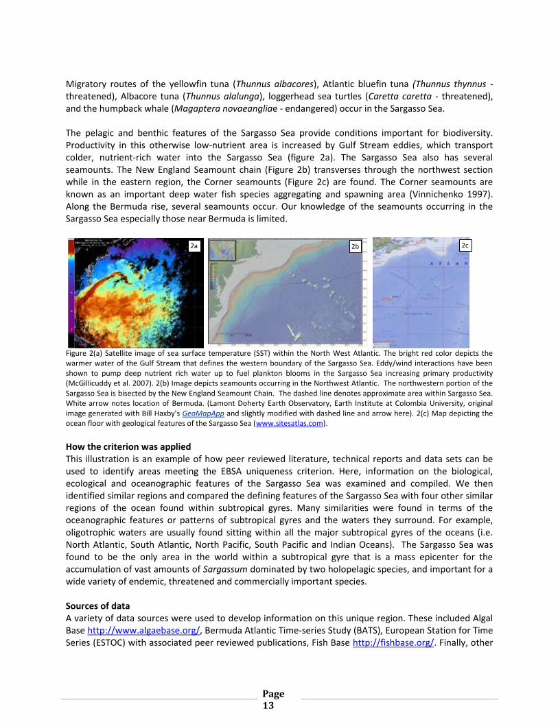
Page 13

Migratory routes of the yellowfin tuna (Thunnus albacores), Atlantic bluefin tuna (Thunnus thynnus - threatened), Albacore tuna (Thunnus alalunga), loggerhead sea turtles (Caretta caretta - threatened), and the humpback whale (Magaptera novaeangliae - endangered) occur in the Sargasso Sea. The pelagic and benthic features of the Sargasso Sea provide conditions important for biodiversity. Productivity in this otherwise low-nutrient area is increased by Gulf Stream eddies, which transport colder, nutrient-rich water into the Sargasso Sea (figure 2a). The Sargasso Sea also has several seamounts. The New England Seamount chain (Figure 2b) transverses through the northwest section while in the eastern region, the Corner seamounts (Figure 2c) are found. The Corner seamounts are known as an important deep water fish species aggregating and spawning area (Vinnichenko 1997). Along the Bermuda rise, several seamounts occur. Our knowledge of the seamounts occurring in the Sargasso Sea especially those near Bermuda is limited.

Figure 2(a) Satellite image of sea surface temperature (SST) within the North West Atlantic. The bright red color depicts the warmer water of the Gulf Stream that defines the western boundary of the Sargasso Sea. Eddy/wind interactions have been shown to pump deep nutrient rich water up to fuel plankton blooms in the Sargasso Sea increasing primary productivity (McGillicuddy et al. 2007). 2(b) Image depicts seamounts occurring in the Northwest Atlantic. The northwestern portion of the Sargasso Sea is bisected by the New England Seamount Chain. The dashed line denotes approximate area within Sargasso Sea. White arrow notes location of Bermuda. (Lamont Doherty Earth Observatory, Earth Institute at Colombia University, original image generated with Bill Haxby's GeoMapApp and slightly modified with dashed line and arrow here). 2(c) Map depicting the ocean floor with geological features of the Sargasso Sea (www.sitesatlas.com).

How the criterion was applied This illustration is an example of how peer reviewed literature, technical reports and data sets can be used to identify areas meeting the EBSA uniqueness criterion. Here, information on the biological, ecological and oceanographic features of the Sargasso Sea was examined and compiled. We then identified similar regions and compared the defining features of the Sargasso Sea with four other similar regions of the ocean found within subtropical gyres. Many similarities were found in terms of the oceanographic features or patterns of subtropical gyres and the waters they surround. For example, oligotrophic waters are usually found sitting within all the major subtropical gyres of the oceans (i.e. North Atlantic, South Atlantic, North Pacific, South Pacific and Indian Oceans). The Sargasso Sea was found to be the only area in the world within a subtropical gyre that is a mass epicenter for the accumulation of vast amounts of Sargassum dominated by two holopelagic species, and important for a wide variety of endemic, threatened and commercially important species. Sources of data A variety of data sources were used to develop information on this unique region. These included Algal Base http://www.algaebase.org/, Bermuda Atlantic Time-series Study (BATS), European Station for Time Series (ESTOC) with associated peer reviewed publications, Fish Base http://fishbase.org/. Finally, other

2b 2c 2a

http://www.marine-geo.org/geomapapp/

http://www.sitesatlas.com/

http://www.algaebase.org/

http://fishbase.org/

Page 14

peer reviewed literature and technical reports were also used. It is important to note that the uniqueness criterion is broad in scope and does not lend itself to one discrete data set (for example, the home range of one species). Instead the distribution, ecology and life history of several species, populations and communities were examined as well as their habitats in tandem with the oceanographic features of the Sargasso Sea. Important considerations Widely recognized, the North Atlantic subtropical gyre and the Sargasso Sea is arguably one of the most well studied subtropical gyres and regions in the ocean (Mouriño-Carballido and Neuer 2008). Hence more information on this area (the gyre and the waters lying within) and lack of information on the other less studied subtropical gyres could lead to perceived uniqueness. It should be noted, though, that the uniqueness criterion can be applied at any scale, from global to regional and local, and is dependent on best available scientific information. In the case of the Sargasso Sea, the uniqueness criterion is met on the global scale because no other area of the world’s oceans have, thus far, been identified as centers of distribution of holopelagic Sargassum drift algae. Given the amount of global monitoring now in place, through satellites and other remote technologies, it is highly unlikely any other similar places of the scale and importance of the Sargasso Sea exist, awaiting discovery. In accordance with the rationale for the CBD uniqueness criteria (annex 1, decision IX/20), the loss of Sargassum weed habitat would likely mean the loss of, or reduction in, important endemic species and threatened sea turtles.

CREDIT: S.A. McKenna, IUCN WCPA Marine - Caribbean Working Group, IUCN WCPA, High Seas MPA Task Force Deep Search Foundation and A. H. Hemphill, IUCN WCPA, High Seas MPA Task Force, Center for Ocean Solutions, Stanford University References Carr, A. and A. B. Meylan. 1980. Evidence of passive migration of green turtle hatchlings in Sargassum. Copeia 1980(2):366-368. Conover, J.T. and J.M. Sieburth. 1964. Effect of Sargassum distribution on its epibiota and antibacterial activity. Botanica Marina 6: 147-157 Coston-ClementsL, Settle LR, Hoss DE& Cross FA. 1991. Utilization of the Sargassum habitat by marine invertebrates and vertbrates - a review. NOAA Technical Memorandum NMFS-SEFSC-296, 30p Friedland, K. D., Miller, M. J., and Knights, B. 2007. Oceanic changes in the Sargasso Sea and declines in recruitment of the European eel. – ICES Journal of Marine Science, 64: 519–530. Gower, J and King, S. (2008) Satellite Images Show the Movement of Floating Sargassum in the Gulf of Mexico and Atlantic Ocean. Available from Nature Proceedings <http://hdl.handle.net/10101/npre.2008.1894.1> Haney J.C. 1986. Seabird Patchiness in tropical ocean waters: The influence of Sargassum “reefs”. The Auk 103:141-151. Hemphill AH 2005. Conservation on the High Seas-drift algae habitat as an open ocean cornerstone. High Seas Marine Protected Areas. Parks 15(3) 48-56 Lamont Doherty Earth Observatory, Earth Institute at Colombia University http://www.ldeo.columbia.edu/~small/AtlanticSmts/pages/NEsmtsBermuda1.htm Maury M. F., "Physical Geography of the Sea," new edition, New York, 1856, pp. 30, pl. vi.

desk%20top%202CBD%20BDA%20docs/%3chttp:/hdl.handle.net/10101/npre.2008.1894.1%3e

http://www.ldeo.columbia.edu/~small/AtlanticSmts/pages/NEsmtsBermuda1.htm

Page 15

McClintock 2002. Sailing the Sea of Life. http://discovermagazine.com/2002/mar/featsea McGillicuddy et al. 2007 Eddy/Wind Interactions Stimulate Extraordinary Mid-Ocean Plankton Blooms Science 316:1021-1026. http://science.whoi.edu/users/olga/eddies/EDDIES_Project.html Mid-ocean ridges and seamounts: oceanography, ecology, and exploitation Theme Session International Council for the Exploration of the Sea 2008 Annual Science Conference Mouriño-Carballido, B. and S. Neuer 2008. Regional Differences in the Role of Eddy Pumping in the North Atlantic Subtropical Gyre: Historical Conundrums Revisited. Oceanography 21(2):52-61 Steinberg DK, Carlson CA, Bates NR, Johnson RJ, Michaels AF, Knap AH 2001. Overview of the US JGOFS Bermuda Atlantic Time-series Study (BATS): a decade-scale look at ocean biology and biogeochemistry Deep-Sea Research II 48 1405}1447 Stevenson, J.J. 1910. Special Articles: The Sargasso Sea. Science VOL. XXXII. No. 832 841-843 Vinnichenko VI 1997. Russian Investigations and Deep Water Fishery on the Corner Rising Seamount in Subarea 6 NAFO Sci. Coun. Studies, 30: 41–49 (East Sargasso sea)

http://discovermagazine.com/2002/mar/featsea

Page 16

Special importance for life history stages of species

Northern elephant seals Short description

Female northern elephant seals undertake a long foraging migration in the North Pacific each year, building a reserve for subsequent months spent fasting on land while giving birth, nourishing a pup, and breeding. Using data from the Tagging of Pacific Predators project (www.topp.org), we identify an area of high female northern elephant seal density during their annual 6-8 month foraging migration, indicating it is an area of special importance for life history stages of this species.

Figure 1. High use open ocean areas of female northern elephant seals during their long migration, July-November, 2004-2007.

Scientific Background Many wide ranging marine animals have an amphibious life history. For example, sea turtles, seabirds, sea lions, and seals spend part of their lives feeding at sea, and part of their lives on land, breeding, caring for young, or molting. In the North Pacific, the northern elephant seal is a wide-ranging top predator with such a life history. Female northern elephant seals haul out on the beaches of the North American west coast twice yearly: once to give birth, nourish young, and breed, and once to molt (Stewart and DeLong 1996). They fast completely during this time. Following each terrestrial visit, northern elephant seals return to sea to feed. They thus undertake a double foraging migration each year - a “short migration” following breeding and a 6-8 month “long migration” following molt. Until recently, it was thought that northern elephant seals were restricted to coastal waters during their migrations; range-maps indicated that elephant seals venture no farther than the continental shelf


Page 17

(Riedman 1990). From the mid-1980s, an advance in tracking technology for obtaining fine-scale data on animal movements allowed for an amazing discovery. During the long migration, female northern elephant seals travel half way across the Pacific, feeding almost entirely in habitats beyond national jurisdiction. They spend more time in some places than others. A robust tracking dataset from 2004-2007 allowed for the identification of multi-individual high-use areas and an analysis of their persistence from year to year. The ecological significance of these areas to northern elephant seal life history is reflected in the energy required to sustain their time on land and ensure pup survival; 48% of their body energy is lost during lactation, and “body reserves obtained during biannual foraging migrations are the most important determinants of reproductive effort in female elephant seals” (Crocker et al. 2001). How the criterion was applied Geographic areas of ecological significance to wide-ranging marine predators can be delineated in several ways. Marine researchers increasingly use techniques that provide a utilization distribution - the relative frequency of locations of an animal or group of animals in a particular area during a given time frame (Van Winkle 1975). The utilization distribution is a probabilistic model describing the relative amount of time that an animal or group of animals spends in any place (Seaman and Powell 1986) and has been particularly useful for identifying areas highly used (or visited) by many individuals (BirdLife International 2004), variably called core areas, high-use areas, and hotspots. Kernel density estimators have emerged as the most commonly used technique for utilization distribution estimation (Worton 1989, Kernohan 2001; BirdLife International 2004; Laver and Kelly 2008), and is the technique we used here. We used the open source software “R” and the kernel density utilization distribution function in the R-package AdeHabitat (Calenge 2006) to calculate and map the utilization distribution of 55 females tracked during their post-molt, long migration in 2004-2007. We focused our analysis on the at-sea portion of the female elephant seal migration (July–November), omitting migration corridors to and from haul-out beaches. Migration corridors are primarily located within Exclusive Economic Zones; most females move quickly through them. We used location data collected from satellite tags deployed as a part of the Tagging of Pacific Predators project (see Sources of Data for more information). Raw Argos satellite positions include a range of inaccurate positions (i.e. positions falling on land, or positions farther away in distance than the animal could possibly have traveled in a given time period). Traditional methods of processing Argos data to remove erroneous positions include simple speed, distance, and angle filters. A more robust approach is a state-space model, a Bayesian statistical approach to accounting for measurement error and estimating the most probably movement pathway (Jonson 2003). We used a state-space model to process raw Argos satellite positions, obtaining the best location estimates given the error distribution of our data. Tracks were interpolated to 4 positions per day. Utilization distributions were calculated for each individual and averaged across years (Figure 1), and within each year (Figure 2), producing a series of volume contours encompassing the area within the average animal spends a given percentage of time. The 95% contour indicates the area where tagged elephant seals spent 95% of their time at sea or, where one is 95% likely to find a tagged elephant seal during the study period. Areas of high use are relatively persistent from year to year (Figure 2). Areas of likely significance were identified using the 50% utilization contour for the utilization distribution averaged across 2004-2007 – those areas of average concentrated use within the home range.

Page 18

Figure 2. Yearly high use open ocean areas of female northern elephant seals during their long migration, July-November, 2004-2007.

Sources of data We used data collected by the Tagging of Pacific Predators project (www.TOPP.org) and provided courtesy of Dr. Daniel P. Costa, University of California, Santa Cruz. TOPP began in 2000 as one of 17 projects of the Census of Marine Life, a 10-year, 80-nation endeavor to assess and explain the diversity and abundance of life in the oceans. TOPP researchers from eight countries began venturing into offshore waters, remote islands, and along rugged coastlines to attach satellite tags to 22 different species of top predators that roam the Pacific Ocean. As of 2007, they have tagged more than 2,000 animals, including elephant seals, white sharks, leatherback turtles, squid, albatross and sooty shearwaters. Molted females were tagged in May-June, 2004-2007 with Wildlife Computers Argos satellite transmitters. Only complete tracks (females that returned to land following their long migration) were used for this analysis: 14, 17, 15, and 9 individuals in 2004-2007 respectively (total n=55). To understand patterns of space-use in years not sampled and under environmental conditions not included in the sampling period (for example, El Nino events), tracking data may be combined with previous publications, expert opinion, habitat models, and at-sea sighting and observation data when available. Important considerations Aarts (2008) summarized a number of important statistical and technical considerations when using tracking data to identify important habitats for marine predators. Considerations in applying kernel density estimators to tracking data were reviewed by Kernhohan et al. (2001), Getz and Wilmers (2004) and Laver and Kelly (2008). In marine environments, habitats move, and they can do so on decadal, yearly, monthly, even daily and hourly time scales. Habitat use and patterns of animal movement are influenced by spatial and temporal resource availability, physiological limits, predator avoidance, and human disturbance. Large-scale episodic phenomena such as the El Niño Southern Oscillation (ENSO) can have large effects on where northern elephant seals spend their time and on reproductive success and pup survival (Le Boeuf and Crocker 2005). Because use of space by marine predators can be dynamic, the best tracking datasets for identifying areas important to the life histories of these animals will span multiple years under a range of ecological and anthropogenic influences and include a sample size large enough to be robust to individual variation. The TOPP northern elephant seal datasets is one of the best in this regard, but even five years


Page 19

of very good data about a relatively small subset of the total population may be few when placing these results in a context of climatic and population level phenomena. CREDIT: A-L. Harrison, University of California at Santa Cruz, Dan Costa’s Lab References Aarts G., MacKenzie M., McConnell B., Fedak M., Matthiopoulos J. 2008. Estimating space-use and habitat preference from wildlife telemetry data. Ecography. 31:140–160. BirdLife International. 2004. Tracking ocean wanderers: the global distribution of albatrosses and petrels. Cambridge, UK: BirdLife International. Available online at: http://www.birdlife.org/action/science/species/seabirds/tracking.html Calenge, C. 2006. The package adehabitat for the R software: a tool for the analysis of space and habitat use by animals. Ecological Modelling 197: 516–519. Crocker D.E, Williams J.D, Costa D.P, Le Boeuf B.J. 2001. Maternal traits and reproductive effort in northern elephant seal. Ecology. 82: 3541–3555. Getz, W. M. and C. C. Wilmers. 2004. A local nearest-neighbor convex-hull construction of home ranges and utilization distributions. Ecography. 27: 489-505. Jonsen I.D., Myers R.A., and Mills Flemming, J. 2003. Meta-analysis of animal movement using state-space models. Ecology 84:3055-2063 Laver, P.N., and Kelly M.J. 2008. A critical review of home range studies. Journal of Wildlife Management. 72:290-298. Le Boeuf, B.J. and Crocker D.E. 2005. Ocean climate and seal condition. Biomed Central Biology. 3: 9 Kernohan, B.J., R.A. Gitzen, and J.J. Millspaugh. 2001. Analysis of animal space use and movements. Pages 125-166 in Radio Tracking and Animal Populations (J.J. Millspaugh and J.M. Marzluff, Eds.). Academic Press, London. Riedman, M. 1990. Pinnipeds: Seals, Sea Lions, and Walruses. Berkeley: University of California Press. Stewart, B.S. and R.L. DeLong. 1995. Double migrations of the northern elephant seal, Mirounga angustirostris. Journal of Mammalogy 76(11): 196-205. Worton, B.J. 1989. Kernel methods for estimating the utilization distribution in home-range studies. Ecology 70: 164-168.

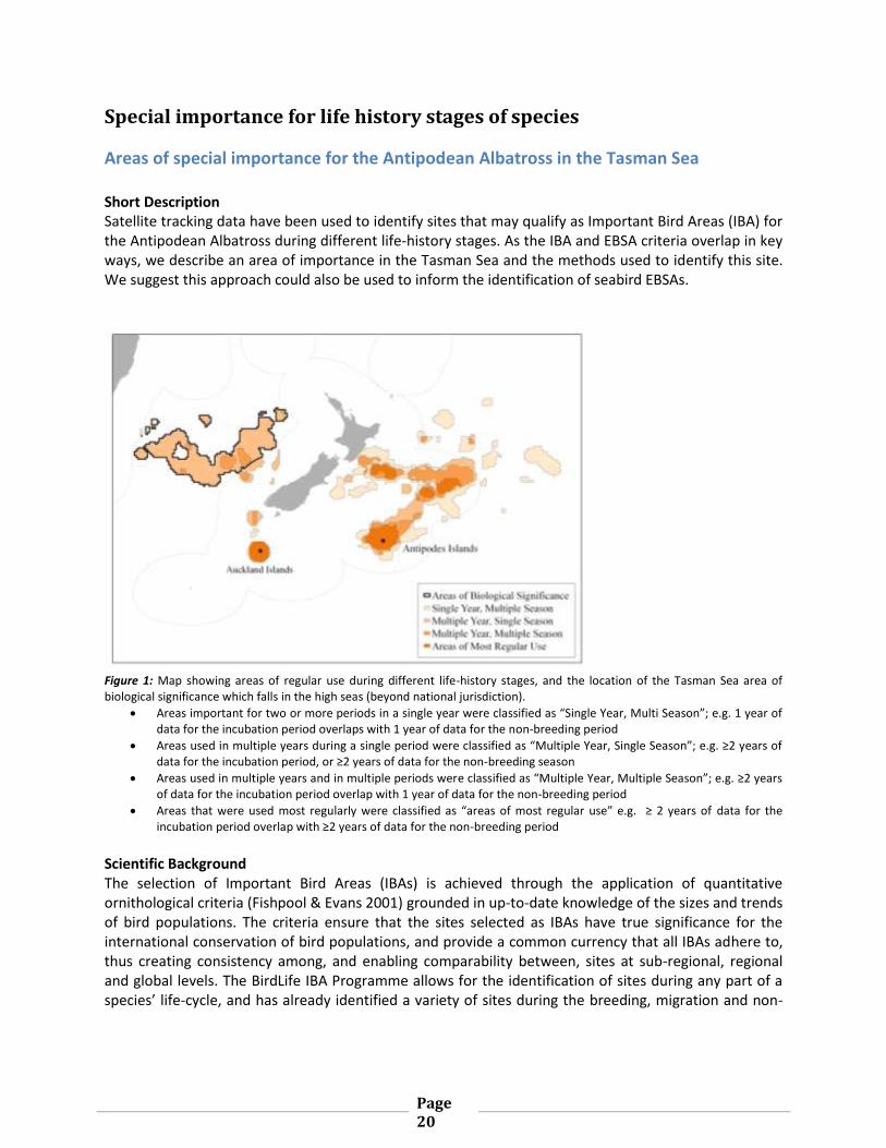
http://www.birdlife.org/action/science/species/seabirds/tracking.html

Page 20


Areas of special importance for the Antipodean Albatross in the Tasman Sea

Short Description Satellite tracking data have been used to identify sites that may qualify as Important Bird Areas (IBA) for the Antipodean Albatross during different life-history stages. As the IBA and EBSA criteria overlap in key ways, we describe an area of importance in the Tasman Sea and the methods used to identify this site. We suggest this approach could also be used to inform the identification of seabird EBSAs.

Figure 1: Map showing areas of regular use during different life-history stages, and the location of the Tasman Sea area of biological significance which falls in the high seas (beyond national jurisdiction).

Areas important for two or more periods in a single year were classified as “Single Year, Multi Season”; e.g. 1 year of data for the incubation period overlaps with 1 year of data for the non-breeding period

Areas used in multiple years during a single period were classified as “Multiple Year, Single Season”; e.g. ≥2 years of data for the incubation period, or ≥2 years of data for the non-breeding season

Areas used in multiple years and in multiple periods were classified as “Multiple Year, Multiple Season”; e.g. ≥2 years of data for the incubation period overlap with 1 year of data for the non-breeding period

Areas that were used most regularly were classified as “areas of most regular use” e.g. ≥ 2 years of data for the incubation period overlap with ≥2 years of data for the non-breeding period

Scientific Background The selection of Important Bird Areas (IBAs) is achieved through the application of quantitative ornithological criteria (Fishpool & Evans 2001) grounded in up-to-date knowledge of the sizes and trends of bird populations. The criteria ensure that the sites selected as IBAs have true significance for the international conservation of bird populations, and provide a common currency that all IBAs adhere to, thus creating consistency among, and enabling comparability between, sites at sub-regional, regional and global levels. The BirdLife IBA Programme allows for the identification of sites during any part of a species’ life-cycle, and has already identified a variety of sites during the breeding, migration and non-

Page 21

breeding periods. In this respect IBA criteria and EBSA criteria have considerable overlap, therefore the data and methodology used to identify IBAs can be used to inform identification of EBSAs. Diomedea antipodensis is one of the largest seabirds on earth, and a member of the great albatross (Diomedea spp.) group. It is endemic to New Zealand, breeding on Antipodes Island (4,635-5,737 pairs), the Auckland Islands group (5,800 pairs on Adams, Disappointment and Auckland), Campbell Island (c.10 pairs), and Pitt Island in the Chatham Islands (one pair since 2004). In 1998, it was estimated that there were approximately 39,000 mature individuals; more recent estimates put this at 25,260 mature individuals. Declines in adult survival, productivity and recruitment are largely due to bycatch in longline tuna fisheries. It is currently listed as Vulnerable by IUCN (BirdLife International, 2009a).

Figure 2: All journeys (n = 173) of Antipodean Albatross tracked using Platform Transmitter Terminal (PTT) devices, attached to 42 birds from Antipodes Island (107 tracks in red) and 30 from Adam Island in the Auckland Islands (65 tracks in blue). Image courtesy of the Global Procellariiform Database. Data provided by Kath Walker (Department of Conservation, New Zealand) and David Nicholls (Chisholm Institute, Australia).

Data from satellite tracking (see figure 2) indicate that birds from the Auckland Islands (subspecies D. a. gibsoni) forage mostly west of New Zealand over the Tasman Sea and south of Australia. Those from the Antipodes Islands (D. a. antipodensis) forage east of New Zealand in the South Pacific, as far as the coast of Chile, and have a larger overall range. The tracking data also show that during different life-history stages birds utilize different areas. To afford full protection to this species it is therefore essential to identify areas important for each life-history stage both within territorial waters and on the high seas, i.e. a network of sites. How the area of special importance to the life history stages of the Antipodean Albatross in the Tasman Sea was identified Of the global IBA criteria, two (A1 and A42) are currently particularly applicable to seabirds in the marine environment. The IBA criteria explicitly mention the demonstration of “regular use” at a site as a necessary requirement for qualification as an IBA. Whenever possible it is important to utilise data from multiple years to provide justification for this. It has been proposed (BirdLife 2009b) that a regularly used hotspot identified solely on tracking data should be required to meet the following conditions: “Areas visited by birds from more than one site or during different periods (seasons or years)”

2 A1. Species of global conservation concern - The site regularly holds significant numbers of a globally threatened species, or other species of

global conservation concern. A4. Congregations - The site is known or thought to hold congregations of ≥1% of the global population of one or more species on a regular or predictable basis. For further details of the IBA Programme please visit: www.birdlife.org/datazone/sites/global_criteria.html

http://www.birdlife.org/datazone/sites/global_criteria.html

Page 22

Figure 3: Density distributions for Antipodean Albatross tracked using Platform Transmitter Terminal (PTT) devices, attached to 42 birds from Antipodes (107 tracks) and 30 from Auckland (65 tracks). The Figure shows the 25, 50, 75 and 100% Utilisation Distributions. Image courtesy of the Global Procellariiform Database. Data provided by Kath Walker (Department of Conservation, New Zealand) and David Nicholls (Chisholm Institute, Australia).

Figure 3 shows areas of greatest use for the tracked Antipodean Albatross population over the course of the study. However, in order to identify sites that are important for the different life-history stages of this species, it is necessary to define the nature and timing of the life-history stages, to divide the tracking dataset accordingly, and to define areas of importance for each stage.

Breeding Season Stages

Return to colony Incubation Hatch Brood-guard Post-guard Fledging

Dec Dec – Feb March-April

March-May May - March the following year

Jan-March (both the following year)

Non-Breeding Season Stages

Successful Breeders Unsuccessful Breeders Juvenile/Immature

March – Dec (the following year) Jan/May - Dec All year (for 5-7 years)

Table 1: Showing dates of different life-history stages of the Antipodean Albatross. Adapted from Brooke (2004)

To determine which areas within the Antipodean Albatross tracking dataset met these conditions of ‘regular use’, the data were split according to the life-history stages outlined in Table 1. This allows identification of sites of importance during both the breeding season (consisting of pre-egg, incubation, brood-guard, and post-guard periods) and non-breeding season. Data were also split for the two different breeding colonies (Antipodes and Auckland islands) because the areas visited by them are different. Within each life-history stage, data were only used if they were available in at least two different years and for a minimum of 4 birds in each year. This is because smaller sample sizes can have an undue influence on the overall areas identified. For each year a Kernel Density Estimation (KDE)3 was applied, Utilisation Distributions (UDs) were calculated, and the 50% UDs were used to represent core areas of activity4. The same process was applied for each life-history stage and each year with sufficient data (see figure 4 for examples). These layers were then combined to create a map of areas of most

3 Other options are available for identifying core areas of activity, though kernel density estimation is one of the

simplest and most effective. See Birdlife (2009b) for detailed comparison of analytical techniques. 4 The 50% utilisation distribution has been commonly used to represent core activities for a number of seabirds,

including the great albatrosses, see BirdLife International (2004).

Page 23

regular use (see Figure 1). Such areas of special importance in the Tasman Sea (Figure 1) can be seen to be important for multiple life-history stages (seasons) in multiple years.

Figure 4: Areas identified as being of most regular use by Antipodean Albatross tracked from the Auckland Islands, during the incubation period (top left); during the brood-guard period (top right); during the non-breeding season (bottom left) and across all life-history stages and years (bottom right). Image courtesy of the Global Procellariiform Database. Data provided by Kath Walker (Department of Conservation, New Zealand) and David Nicholls (Chisholm Institute, Australia).

This example shows that seabirds often congregate at predictable hotspots (see Weimerskirch 2007 for further example), and linking a hotspot to specific static and/or dynamic environmental variables is an important method for determining a sites’ spatial and temporal stability and/or variability. Linking the sites to environmental variables can clarify whether the importance of an area is determined topographically or bathymetrically (e.g. X km either side of the shelf break, or the presence of a seamount) or by environmental variables (e.g. specific sea surface temperatures, currents, or chlorophyll concentrations). This helps define the features that may be in need of protection to sustain the population. Linking sites to these variables will help to determine for which other taxa and habitats the area might also be important (e.g. Edgar et al. 2008)). Walker and Elliott (2006) found that birds tracked from both Auckland and Antipodes preferred to forage at the outer edge of shelves and over seamounts, particularly where there were strong currents or eddies and productivity was enhanced, as well as over deep water. The relationship between these variables would be better understood via habitat modeling which may also help to make extrapolations/predictions to non-surveyed areas (e.g. Clarke et al. 2003; Yen et al. 2004).

Page 24

Sources of data For this illustration, we used tracking data obtained from the Global Procellariiform Tracking Database held by the Global Seabirds Programme of Birdlife International. Data for Antipodean Albatross were provided to the database by Kath Walker (Department of Conservation, New Zealand) and David Nicholls (Chisholm Institute, Australia). The Global Procellariiform Database holds tracking data information provided by 57 scientists from 11 countries on 28 species of albatross and petrels. Up to the end of 2008 it held 3,764 tracks obtained from Platform Transmitter Terminal (PTT) & Global Positioning Satellites (GPS) totaling 957,148 hours at sea, as well as 721 tracks obtained from Geolocators (GLS) totaling 61,832 days. A complete analysis of the Procellariiform database would reveal a number of EBSAs on the high seas. Tracking datasets exist for numerous other seabird species, pinnipeds, cetaceans, turtles and pelagic fish, and the methodologies outlined here could be applicable to these other datasets. (see e.g. Tagging of Pacific Predators (TOPP5), Seaturtle.com, Falabella et al 2009) To conduct the most complete tracking data analysis requires an adequate sample size of tracked birds within each life-history stage. Most seabird species do not have a complete dataset covering all life-history stages; however for many some form of between-years or between-seasons comparison would be possible. Important considerations Identification of biologically significant areas for the various life-history stages of wide-ranging species is inherently linked to the distribution patterns of marine biodiversity and productivity. Seabirds are one of the best taxa for this purpose, because as top predators they are excellent indicators of the state of the wider marine environment, they are easily observed, readily identified and widely surveyed and monitored. In addition they are often linked to a specific range of habitat features, and thus identifying important sites for seabirds is likely to include areas and habitats of importance for a wider range of taxa. Interpreting tracking data is of vital importance in identifying a potential EBSA on the high seas. Care needs to be taken in analysis of data to ensure that a consistent and comparable approach is used to identifying and delimiting sites. The ecology of individual species needs to be considered at all stages of an analysis to ensure that variation is accounted for in the sites identified, and that the species’ ecology is amenable to a site-based approach during each life-history stage. Representative sample sizes are especially important for identification of potential EBSAs based solely on tracking data. Bootstrapping (e.g. Manly 2006) may be a useful method for determining if the sample size of tracked birds is representative of the wider population. Adequate sample sizes are likely to vary greatly between species and geographic regions. For studies with small sample sizes, pseudo-replication can be an issue, as the foraging behaviour of a single individual on a single trip can produce hotspots in regions not frequented by any other individual from the same colony or dataset (Seamen et al. 1999). The possibility of missing hotspots should also be borne in mind when interpreting maps, irrespective of the sample size.

5 www.topp.org

Page 25

Final boundary delineation of EBSAs is always likely to be a difficult choice, and deciding where the boundary should be should include regional and species-specific expertise. It may ultimately be guided by the threats present and the management needs of a given area. CREDIT: Ben Lascelles and Lincoln Fishpool, BirdLife International References BirdLife International (2004). Tracking Ocean Wanderers: the global distribution of albatrosses and petrels. Results from the Global Procellariiform Tracking Workshop, 1-5 September, 2003, Gordon’s Bay, South Africa. Cambridge, UK: Birdlife International. BirdLife International (2009a) Species factsheet: Diomedea antipodensis. Downloaded from www.birdlife.org BirdLife International (2009b). Using seabird satellite tracking data to identify marine IBAs. Report of a workshop 1-3 July 2009. CNRS, Chize, France. UK: Cambridge BirdLife International internal report. Brooke, M. (2004). Albatrosses and Petrels across the World. Oxford: Oxford University Press. Clarke E. D., L. B. Spear, M. L. Mccracken, F. F. C. Marques, D. L. Borchers, S. T. Buckland and D. G. Ainley. (2003). Validating the use of generalized additive models and at-sea surveys to estimate size and temporal trends of seabird populations. Journal of Applied Ecology 40: 278–292. Edgar G.J., P.F. Langhammer, G. Allen, T.M. Brooks, J. Brodie, W. Crosse, N. de Silva, L.D.C. Fishpool, M.N. Foster, D.H. Knox, J.E. Mccosker, R. Mcmanus, A.J.K. Millar and R. Mugo (2008). Key biodiversity areas as globally significant target sites for the conservation of marine biological diversity. Aquatic Conservation: Marine And Freshwater Ecosystems 18: 969–983. Falabella, V., C. Campagna and J.P. Croxall (eds) (2009). Atlas del Mar Patagonico: Especies y Espacias. Edicions del Foro, Buenos Aires. Fishpool L.D.C. and M.L. Evans (eds) (2001). Important Bird Areas in Africa and Associated Islands: priority sites for conservation. Newbury and Cambridge, UK: Pisces Publications and Birdlife International (BirdLife Conservation series No 11). Manly B.F.J., (2006). Randomization, Bootstrap and Monte Carlo Methods in Biology. Taylor & Francis, UK. O’ Brien S.H., R.A. Robinson, S.J. Taylor, and K.W. Gillon (1999). Variability in seabird density. JNCC Report, No. 297. Seaman D.E., J.J. Millspaugh, B.J. Kernohan, G.C. Brundige, K.J. Raedeke and R.A. Gitzen. (1999). Effects of Sample Size on Kernel Home Range Estimates. Journal of wildlife management. Wildlife Management. 63(2):739-747. Walker, K. and G. Elliott (2006). At-sea distribution of Gibson’s and Antipodean wandering albatrosses, and relationships with longline fisheries. Notornis 53(3): 265-290. Weimerskirch H. (2007). Are seabirds foraging for unpredictable resources? Deep-Sea Research II 54: 211–223. Yen P.P.W., F. Huettmann and F. Cooke (2004). A large-scale model for the at-sea distribution and abundance of Marbled Murrelet (Brachyramphus marmoratus) during the breeding season in coastal British Columbia, Canada. Ecological Modeling 171:395–413.

http://www.birdlife.org/

Page 26


Pacific White Sharks

Short Description Adult white sharks tracked from several sites along the North American coast travel to a region in the northeastern Pacific, equidistant between Baja California and Hawaii, where they remain for up to six months. It remains unclear whether these represent breeding or feeding migrations. Scientific Background Due to infrequent, yet often sensational interactions with people, white sharks have long captured the imagination of humans. Most of the studies of white sharks have centered around pinniped rookeries, where adult a white sharks feed on elephant seals and sea lions. Off the coast of northern California, the interactions between pinnipeds and white sharks have been studied at the Farallon Islands and Año Nuevo Island for decades (Ainley et al. 1985). White sharks are present at these islands predominately in the late summer through winter when they feed on young elephant seals and sea lions. Although pinnipeds are present throughout the year, white sharks are apparently only present for a portion of the year and their movement patterns after leaving remained a mystery for decades. With the advent of novel electronic tagging technologies, it has since been possible to track white sharks for periods of up to one year and shed light on their movement patterns after departing pinniped colonies. To better understand the movements of white sharks throughout the year, a tagging program was initiated in 1999 off the Farallon Islands (Boustany et al. 2002, Weng et al. 2007a). Pop-up satellite tags are attached externally to marine animals allowing for attachment without the need for capture, which is useful when dealing with potentially dangerous animals such as white sharks. The tags collect pressure, temperature and light-level data while on the fish and then detach at a preprogrammed date and transmit summaries of stored data to satellites. Pressure readings reveal depth preferences of the tagged animal while light-level and temperature data can be used to reconstruct geolocated tracks. Much to the surprise of white shark researchers, sharks tagged off the coast of California all showed movement far offshore. All sharks showed highly directed movement (> 100 km/day) to the southwest in the winter or spring to the subtropical gyre equidistant between Baja California and the Hawaiian Islands. A small number of sharks maintained movement to the west, eventually ending up in the waters of Hawaii. All sharks remained in these areas until the late summer or early fall, at which point they showed return migrations to the coast of central California, oftentimes to the same small islands from which they were originally tagged. Pop-up tagging conducted at Isla Guadalupe, off the coast of Baja California, Mexico showed similar movement patterns, with most sharks migrating to the same offshore region and several sharks continuing on to the Hawaiian Islands (Domeier and Nasby-Lucas, 2008). While adult sharks from both Mexico and California travel to the same offshore regions, no individuals have yet been observed to travel between pinniped colonies in Mexico and the US.

Page 27

Panels on left from Weng et al. 2007a showing seasonal densities of white sharks tagged off the northern California coast, USA. Panels on the right from Domeier and Nasby-Lucas, 2008 show seasonal densities of white sharks tagged off Baja California, Mexico.

While movement to the Hawaiian Islands is understandable, given the abundant marine mammal prey base, what attracts white sharks to the open ocean area between the continent and Hawaii is less understood. This area overlies a seafloor that is several kilometers deep with few seamounts or other physiographic features of note. Being subtropical, the surface waters are generally warm (22-25o C) with a deep thermocline and little in the way of productivity, eddies, fronts or strong temperature gradients. In addition, few fish or marine mammal resources are known in this area with commercial fish catches for tuna, billfish and sharks all being higher either to the north or to the south of this region. Likewise, whale, dolphin and pinniped densities are all higher, either to the north or south, on in the coastal areas of Hawaii or North America. While in this region, sharks exhibited frequent deep diving (> 700 m) experiencing a wide range of temperatures (4-27o C). These offshore movements stand in contrast to migration patterns exhibited by juvenile white sharks. One to three year old white sharks electronically tracked off the North American coast showed only coastal movements, remaining near shore in the waters of Southern California and Northern Mexico (Weng et al. 2007b). These waters are known nursery areas for young of the year and juvenile white sharks where they feed on fish before making the transition to feeding on marine mammals as they mature. There are several hypotheses regarding why white sharks exhibit offshore migrations to this specific region of the northeast Pacific. It is possible that this area serves as a pupping ground, where female white sharks give birth in an area that is warm and low in predators, increasing survivorship of young sharks. These young white sharks could then travel towards the nursery areas along the North American coast sometime in their first year of life. Both male and female sharks travel to this region, suggesting that it does not constitute only a pupping ground, as males would have no need to migrate there if that was the case. It remains possible that this area serves as both a pupping and breeding ground, providing the gestation period is approximately 12 months long. In such a scenario, males would mate with females shortly after the females give birth. It also remains possible that this is a foraging area for adult white sharks. The extended period of time that sharks remain in this region, up to 9 months, and extensive diving patterns observed while sharks are there, suggest foraging. With few marine mammal resources known from this region, it remains unclear what prey items white sharks would be targeting. As such, even after a decade of tracking white sharks to this area, it is still unknown why they travel to this region. However, given the fact that all adult sharks tagged off the North American coast travel to

Page 28

and spend a considerable amount of time in this area, it can safely be stated that this region is important for the ecology of white sharks in the North Pacific. How the criterion was applied Both studies used diving and movement data returned from the tags to discern different behavioral patterns exhibited by the sharks. Diving patterns changed abruptly as sharks moved from the coastal waters and began their migrations to the west. Daily dive depths increased from less than 70 m to greater than 500 m as sharks left the pinniped rookeries in the early winter. During the migration phase, time spent at the surface also changed dramatically. While hunting for seals and sea lions nearshore, sharks spent very little time (<25%) in the top 5 m but as they moved offshore time spent in the surface waters increased dramatically (>50%), possibly to allow for celestial geolocation by the sharks (Weng et al. 2007a, Domeier and Nasby-Lucas, 2008). In addition to diving behavior, horizontal movement patterns were also used to delineate different regions and behaviors in the seasonal cycle of white sharks. Both studies used longitudinal movements to identify when sharks began their offshore migrations and when they arrived to the presumed offshore foraging area. It was therefore possible to identify migratory corridors as well as foraging regions. In addition, it is possible to calculate utilization distributions for white sharks for both the nearshore and offshore phases of their lives. Weng et al (2007a) used the kernel density method (Silverman 1986) to identify specific areas of high use by the tagged sharks. Tracks were regularized to one position per day and all the resulting points were broken down into meteorological seasons. Spring and summer seasons corresponded with the offshore component of the white shark’s annual cycle. Both studies also calculated 25, 50 and 95% utilization distributions, with the 25% contour identified as the core region of habitat utilization. Utilization distributions were calculated using the home range extension (Rodgers & Carr 1998) for ArcView 3.2 (ESRI).

Sources of Data Although animal observation data can be difficult and expensive to collect for open-ocean species, several sources exist to serve these data after they have already been collected. The Tagging of Pacific Predators project (TOPP) is one of the largest electronic tracking projects in the world. To date, researchers associated with this project have tagged over 2000 individual animals in the North Pacific Ocean. Twenty-two different species, including elephant seals, white sharks, leatherback turtles, Humboldt squid, albatross and sooty shearwaters have been tracked and data can be viewed online through the TOPP website (http://www.topp.org/). Beyond serving only electronic tag data, several programs are currently consolidating all types of marine animal observation data, including data from surveys, fishery catch data and tagging data. The Ocean Biogeographic Information System (OBIS) has set up an online portal where researchers can upload and download any marine species observation data (http://www.iobis.org/). They currently have over 19 million individual sightings from over 106,000 marine species from 660 databases. While the OBIS program deals exclusively with marine species, the Global Biodiversity Information Facility (GBIF) performs a similar service for both marine and terrestrial species (http://www.gbif.org/). The GBIF program currently has over 180 million records from over 8,000 individual datasets. From all these websites, it is possible to contact individual researchers in order to gain access to data for scientific purposes. CREDIT: A. Boustany, Duke University Marine Geospatial Ecology Lab


http://www.iobis.org/

http://www.gbif.org/

Page 29

References Ainley DG, Henderson RP, Huber HR, Boekelheide RJ, Allen SG, McElroy TL (1985) Dynamics of white shark/pinniped interactions in the Gulf of the Farallones. Mem South Calif Acad Sci 9:109–122

Boustany AM, Davis SF, Pyle P, Anderson SD, Le Boeuf BJ, Block BA (2002) Expanded niche for white sharks. Nature 415:35–36 Domeier ML, Nasby-Lucas N (2008) Migration patterns of white sharks Carcharodon carcharias tagged at Guadalupe Island, Mexico, and identification of an eastern Pacific shared offshore foraging area. Mar Ecol Prog Ser 370:221–237 Rodgers AR, Carr AP (1998) HRE: The home range extension for ArcView. Ontario Ministry of Natural Resources, Centre for Northern Forest Ecosystem Research, Thunder Bay Silverman B (1986) Density estimation for statistics and data analysis. Chapman & Hall, London, New York Weng KC, Boustany AM, Pyle P, Anderson SD, Brown A, Block BA (2007a) Migration and habitat of white sharks (Carcharodon carcharias) in the eastern Pacific Ocean. Mar Biol 152:877–894 Weng KC, O’Sullivan JB, Lowe CG, Winkler CE, Dewar H, Block BA (2007b) Movements, behavior and habitat preferences of juvenile white sharks Carcharodon carcharias in the eastern Pacific. Mar Ecol Prog Ser 338:211–224

Page 30

Importance for threatened, endangered or declining species and/or

habitats

Critically Endangered Pacific Leatherback Sea Turtles

Short Description New tracking technologies have allowed researchers to examine the movements of the critically endangered Pacific Leatherback turtle. Several years of tracking have revealed a consistent foraging area for leatherback turtles in the South Pacific Gyre.

Figure1: Reproduced from Shillinger et al. 2008. Panel A: daily swimming speed of tracked turtles as they moved to the south from the tagging area in Costa Rica. Panel B: Tracks of tagged turtles plotted over eddy kinetic energy, red indicates high energy regions and white indicates low energy regions. Panel C: Turtle tracks plotted over chlorophyll concentration, green areas indicating highest chlorophyll levels.

Scientific Background Studying pelagic species on the high seas has traditionally been difficult. The large distances from shore coupled with the highly mobile nature of the organisms have precluded direct observation. Recent technological advances have permitted researchers to track highly migratory pelagic species by allowing data collection and transmission remotely (Eckert, 2006). These novel electronic tags have been particularly useful for studies involving air-breathing animals in the open ocean, as frequent surfacing allows for direct uplinks to satellites, and animals can therefore be tracked in near real time. While the data these tags have returned is invaluable in shedding light on the basic biology of pelagic species, they gain even more importance when addressing questions pertaining to conservation of severely threatened and endangered species. A prime example of this is the recent electronic tracking conducted on leatherback turtles in the eastern Pacific Ocean. Like many marine turtle species, the slow growth and low reproductive potential of leatherback turtles makes them particularly sensitive to excessive mortality of adult life stages. Leatherbacks in the eastern Pacific Ocean have suffered through illegal poaching and egg collecting on the nesting beaches, resulting in severe population declines. Surveys at nesting beaches in Costa Rica and southern Mexico have seen numbers decline by over 90% in the last 20 years and these populations are now recognized as critically endangered (Spotila et al. 2000). Ongoing conservation efforts have decreased land based mortality, yet

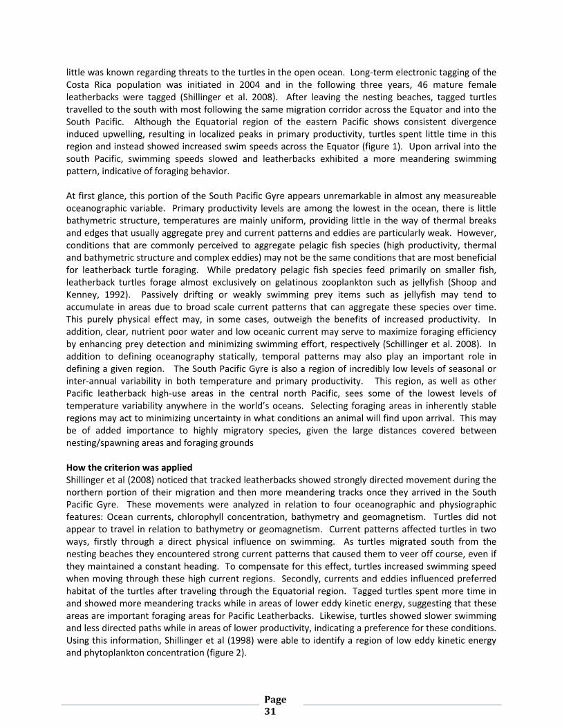
Page 31

little was known regarding threats to the turtles in the open ocean. Long-term electronic tagging of the Costa Rica population was initiated in 2004 and in the following three years, 46 mature female leatherbacks were tagged (Shillinger et al. 2008). After leaving the nesting beaches, tagged turtles travelled to the south with most following the same migration corridor across the Equator and into the South Pacific. Although the Equatorial region of the eastern Pacific shows consistent divergence induced upwelling, resulting in localized peaks in primary productivity, turtles spent little time in this region and instead showed increased swim speeds across the Equator (figure 1). Upon arrival into the south Pacific, swimming speeds slowed and leatherbacks exhibited a more meandering swimming pattern, indicative of foraging behavior. At first glance, this portion of the South Pacific Gyre appears unremarkable in almost any measureable oceanographic variable. Primary productivity levels are among the lowest in the ocean, there is little bathymetric structure, temperatures are mainly uniform, providing little in the way of thermal breaks and edges that usually aggregate prey and current patterns and eddies are particularly weak. However, conditions that are commonly perceived to aggregate pelagic fish species (high productivity, thermal and bathymetric structure and complex eddies) may not be the same conditions that are most beneficial for leatherback turtle foraging. While predatory pelagic fish species feed primarily on smaller fish, leatherback turtles forage almost exclusively on gelatinous zooplankton such as jellyfish (Shoop and Kenney, 1992). Passively drifting or weakly swimming prey items such as jellyfish may tend to accumulate in areas due to broad scale current patterns that can aggregate these species over time. This purely physical effect may, in some cases, outweigh the benefits of increased productivity. In addition, clear, nutrient poor water and low oceanic current may serve to maximize foraging efficiency by enhancing prey detection and minimizing swimming effort, respectively (Schillinger et al. 2008). In addition to defining oceanography statically, temporal patterns may also play an important role in defining a given region. The South Pacific Gyre is also a region of incredibly low levels of seasonal or inter-annual variability in both temperature and primary productivity. This region, as well as other Pacific leatherback high-use areas in the central north Pacific, sees some of the lowest levels of temperature variability anywhere in the world’s oceans. Selecting foraging areas in inherently stable regions may act to minimizing uncertainty in what conditions an animal will find upon arrival. This may be of added importance to highly migratory species, given the large distances covered between nesting/spawning areas and foraging grounds How the criterion was applied Shillinger et al (2008) noticed that tracked leatherbacks showed strongly directed movement during the northern portion of their migration and then more meandering tracks once they arrived in the South Pacific Gyre. These movements were analyzed in relation to four oceanographic and physiographic features: Ocean currents, chlorophyll concentration, bathymetry and geomagnetism. Turtles did not appear to travel in relation to bathymetry or geomagnetism. Current patterns affected turtles in two ways, firstly through a direct physical influence on swimming. As turtles migrated south from the nesting beaches they encountered strong current patterns that caused them to veer off course, even if they maintained a constant heading. To compensate for this effect, turtles increased swimming speed when moving through these high current regions. Secondly, currents and eddies influenced preferred habitat of the turtles after traveling through the Equatorial region. Tagged turtles spent more time in and showed more meandering tracks while in areas of lower eddy kinetic energy, suggesting that these areas are important foraging areas for Pacific Leatherbacks. Likewise, turtles showed slower swimming and less directed paths while in areas of lower productivity, indicating a preference for these conditions. Using this information, Shillinger et al (1998) were able to identify a region of low eddy kinetic energy and phytoplankton concentration (figure 2).

Page 32

. Figure2: Reproduced from Shillinger et al. 2008. Colors from red to yellow show the density utilization distribution of tracked leatherback turtles with red areas being the regions with the highest utilization. The green outline highlights the region identified as having particularly low primary productivity and eddy kinetic energy.

Sources of Data Turtle track data were obtained by tagging turtles with either Sea Mammal Research Unit (SMRU) Satellite Relay Data Logger (SRDL) tags or Wildlife Computer, Smart Position Only (SPOT) tags. Both these tag types uplink to ARGOS satellites when the turtles surface, providing information on the position of the animal. The SRDL tags also collect and transmit temperature, dive data, and tag diagnostic information. Oceanographic and physiographic data were obtained through freely available sources. Chlorophyll data were obtained from the Sea-viewing Wide Field-of-view Sensor (SeaWiFS) satellite, the ocean current data through the Archiving, Validation, and Interpretation of Satellite Oceanographic data (Aviso) project satellites, bathymetry came from the Smith and Sandwell (1997) global bathymetry dataset and geomagnetic data were obtained through the International Geomagnetic Reference Field (IGRF-10) dataset.

Important Considerations When trying to identify ecologically and biologically significant areas based on marine animal tracking data, it is important to delineate different behavior patterns throughout the track. Some animals show a distinct migratory phase consisting of highly directional travel and a foraging phase that shows more circuitous movement paths. In the case of Pacific leatherbacks, migration corridors were found in the region between the nesting beaches and the Equator. This corridor was limited in both its spatial extent as well as the timing of migration. In addition, it was possible to identify a specific region of the South Pacific Gyre as an important foraging region for these turtles. Although the South Pacific Gyre appears unremarkable based on the criteria we normally choose to define ecologically and biologically significant areas (high productivity, complex bathymetry, and major current patterns), migrations over three tagging years showed to be a consistent foraging area for leatherback turtle populations in the eastern Pacific. The high number of turtles tracked to this region over multiple years can give us confidence that this region is vital to post nesting leatherback turtles. These findings show that, by letting animals of interest show us what regions are important to them, it is possible to define EBSAs even in regions that we may not have originally thought were significant. CREDIT: A. Boustany, Duke University Marine Geospatial Ecology Lab

Page 33

References Eckert SA (2006) High-use oceanic areas for Atlantic leatherback sea turtles (Dermochelys coriacea) as identified using satellite telemetered location and dive information. Mar Biol 149: 1257–1267 Shillinger GL, Palacios DM, Bailey H, Bograd SJ, Swithenbank AM, Gaspar P, Wallace BP, Spotila JR, Paladino FV, Piedra R, Eckert SA, Block BA (2008) Persistent leatherback turtle migrations present opportunities for conservation. PLOS Biol 6: 1408-1416 Shoop CR, Kenney RD (1992) Seasonal distribution and abundances of loggerhead and leatherback sea turtles in waters of the northeastern United States. Herpetol Monogr 6:1–67 Smith WHF, Sandwell DT (1997) Global seafloor topography from satellite altimetry and ship depth soundings. Science 277: 1957–1962. Spotila JR, Reina RD, Steyermark AC, Plotkin PT, Paladino FV (2000) Pacific leatherback turtles face extinction. Nature 405: 529–530.

Page 34


habitats

Establishing at-sea habitat preferences as a means of delineating EBSAs for threatened

species: an example of the identification of Important Bird Areas (IBAs) in the Bering

Sea for the Short-tailed Albatross

Short Description Integrating different distributional datasets (especially from remote-recording instruments and at-sea surveys) is likely to be important in identifying EBSAs for a variety of top predators found on the high seas. In this example we look at how satellite tracking data and vessel survey data can be used to identify IBAs based on habitat preferences for a threatened seabird, the Short-tailed Albatross.

Figure 1: Map of candidate IBA for the Short-tailed Albatross at the Bering Sea shelf break. This map shows “areas of regular use” identified from satellite tracking data, vessel survey data, and a 70km buffer around suitable topography (1000m < Depth>250m and slope>2.5degrees) that could be used to define the boundary of the IBA.

Scientific background BirdLife International is the IUCN Red List authority for birds, and conducts a comprehensive review of the status of all species ever four years, with annual reviews of the most threatened. The BirdLife Important Bird Areas (IBA) Programme uses the Red List assessment to define one of the global IBA criteria for identifying IBAs (Category A1), such that sites critical for the conservation of the most threatened species are identified.6 6 A1. Species of global conservation concern - The site regularly holds significant numbers of a globally threatened species, or other species of

global conservation concern. For further details of the IBA Programme please visit: www.birdlife.org/datazone/sites/global_criteria.html

http://www.birdlife.org/datazone/sites/global_criteria.html

Page 35

The IBA criteria explicitly require the demonstration of “presence of significant numbers of birds” and the “regular use” at a site in order for it to qualify as an IBA. Whenever possible, data from multiple years are used to provide justification. The Short-tailed Albatross (Phoebastria albatrus) breeds on the island of Torishima (Japan), and on Minami-kojima in the Senkaku Islands (claimed by Japan, the People's Republic of China and the Republic of China on Taiwan). Historically, there are believed to have been at least nine colonies to the south of Japan and in the East China Sea. The species declined dramatically during the 19th and 20th centuries, and was believed extinct in 1949, until rediscovered in 1951. The current population is estimated to be 2,364 individuals, with 1,922 birds on Torishima and 442 birds on Minami-kojima (BirdLife International 2009a). Satellite tracking has indicated that during the breeding season (December - May) it is found in highest densities around Japan. In the post-breeding season, and for sub-adults during the entire year, its marine range covers most of the northern Pacific Ocean, but it occurs in highest densities in areas of upwelling along shelf waters of the Pacific Rim (Suryan et al. 2006). During the post-breeding period females spend most of their time in shelf waters of the Exclusive Economic Zones (EEZ) belonging to Japan and Russia, while males and juveniles spend their time in similar habitats in the EEZs around the Aleutian Islands, Bering Sea and the coast of North America. This species is currently listed as Vulnerable (BirdLife International 2009a) because, although conservation efforts have resulted in a steady population increase (US Fish & Wildlife Service 2008), it has a very small breeding range, rendering it highly susceptible to stochastic events and human impacts. Away from the breeding colonies mortality caused by fisheries is a major threat, and environmental contaminants at sea (oil-based compounds) may also be an issue. Threats at sea are exacerbated by the fact that birds concentrate at predictable hotspots. This example looks at the methods available for determining where these predictable hotspots are located, and what environmental variables may be responsible for them. Although we focus on the Short-tailed Albatross, which is mostly tied to the EEZs of several nations, the methodologies are applicable to any threatened oceanic top predator that occurs at predictable hotspots, including those on the high seas. How the criterion was applied It has been proposed (BirdLife 2009b) that a regularly used hotspot identified solely on tracking data should be required to meet the following conditions: “Areas visited by birds from more than one site or during different periods (seasons or years)”

To determine the areas within the Short-tailed Albatross tracking dataset that met these conditions of ‘regular use’, the data were split according to season. This allows us to identify sites of importance during both the breeding and non-breeding seasons. Within each season, data were only used if they were available in at least two different years and for a minimum of 4 birds in each year. This is because smaller sample sizes can have an undue influence on the overall areas identified. For each year a Kernel

http://en.wikipedia.org/wiki/People%27s_Republic_of_China

http://en.wikipedia.org/wiki/Republic_of_China

http://en.wikipedia.org/wiki/Taiwan

Page 36

Density Estimation (KDE)7 was applied, Utilisation Distributions (UDs) were calculated, and the 50% UDs were used to represent core areas of activity8. The same process was applied for each life-history stage and each year with sufficient data. These layers were then combined to create a map of ‘regular use’ and the number of tracked birds visiting each site was determined (see Figure 2)

Figure 2: Map of tracking data showing areas of ‘regular use’ during different seasons, and the number of tracked birds using each area (numbers on map). Areas outside of the ‘regular use’ sites had up to 6 birds using them, though they did not do so repeatedly.

Opportunistic at-sea sightings of Short-tailed Albatross were compiled from vessel-based observations in the North Pacific (Pacific Pelagic Seabird Database 2007) for the years 1994 – 2004. The data indicate the location of sightings and the number of birds seen on each occasion, but the dataset represents presence-only data, and has not been compiled from standardised, systematic surveys, so has limitations. However, it represents a useful additional, comparative dataset from which certain inferences can be made of the number of birds likely to be using an area of ‘regular use’ identified from the tracking data. The vessel data were overlaid with a 1 degree square grid9 and the maximum group size of birds sighted within each cell was calculated. The number of years for which a cell had positive sightings was also calculated to investigate consistency between years. It is clear that some areas, such as that in the Bering Sea and the middle of the Aleutian Chain, have higher counts of Short-tailed Albatross than others. However, because of the opportunistic nature of the vessel sightings it is difficult to delimit areas based on these data alone. Conversely, while tracking data do allow areas to be delimited, they do not enable estimates of abundance to be made. Using a combination of both data sources it is possible to delimit areas and determine their overall importance based on the number of birds present. Integrating satellite tracking data and vessel survey data has proved a successful method for identifying and delimiting IBAs in Portugal (Ramirez et al. 2008) and Spain (SEO/BirdLife 2009).

7 Other options are available for identifying core areas of activity, though kernel density estimation is one of the

simplest and most effective. See BirdLife International (2009b) for detailed comparison of analytical techniques. 8 The 50% utilisation distribution has been commonly used to represent core activities for a number of seabirds,

including the great albatrosses, see BirdLife International (2004). 9 A 1 degree square was used for the kernel analysis of the tracking data, so using this size as the basis for the

grid allows comparisons of the dataset to be made.

Page 37

Figure 3: Map showing areas of ‘regular use’ during different seasons (identified from tracking data), the maximum number of birds counted within a 1 degree square obtained from opportunistic at-sea sightings, and the number of years a sighting was made within each square between 1994 and 2004.

Suryan et al. (2006) conducted first-passage time analysis (FPT; Fauchald & Tveraa 2003) on Short-tailed Albatross tracked in the Aleutian Islands to reveal the location and spatial scale of area restricted search (ARS) patterns. They found that, on average, ARS occurred within a 70km radii, which means that once an area of suitable habitat has been found, searching occurs within 70km of this point. To ensure that adequate habitat is included in hotspots identified, boundaries of these sites should therefore include a 70km buffer either side of suitable habitats, which is illustrated in Figure 1. In Figure 1, showing the Bering Sea shelf break IBA, 8 of the 41 tracked birds (20%) were found to use this area extensively, with birds present between June and November. The vessel survey data agree with this, with most sightings in June and September. The seasonality of occurrence here can be partly explained by the fact that the ocean in these latitudes is covered by sea ice at other times of the year. In this example both the tracking data and the vessel data indicate that birds are congregating around the shelf break between 250 and 1000m depth. The shelf within this area has a maximum 21° slope angle, and the mean annual water temperature is around 1°C. Suryan et al. (2006) also confirmed the importance of the shelf break and slope regions as hotspots of activity. They also found that at all scales, wind speed, depth, slope, and chlorophyll a had a significant effect on FPT. This example shows a method for identifying key habitats for a threatened species in territorial waters; similar methods could be applied to threatened species on the high seas to identify potential EBSAs.

Sources of data For this illustration, we used tracking data obtained from the Global Procellariiform Tracking Database held by the Global Seabirds Programme of Birdlife International. Data for Short-tailed Albatross were provided to the database by Dr Rob Suryan (Oregon State University, USA). The Global Procellariiform Database holds tracking data information provided by 57 scientists from 11 countries on 28 species of albatross and petrels. Up to the end of 2008 it held 3,764 tracks obtained from Platform Transmitter Terminal (PTT) & Global Positioning Satellites (GPS) totaling 957,148 hours at

Page 38

sea, as well as 721 tracks obtained from Geolocators (GLS) totaling 61,832 days. A complete analysis of the Procellariiform database would reveal a number of EBSAs on the high seas. Tracking datasets exist for numerous other seabird species, pinnipeds, cetaceans, turtles and pelagic fish, and the methodologies outlined here could be applicable to these other datasets. (see e.g. Tagging of Pacific Predators (TOPP10), Seaturtle.com, Falabella et al 2009) To conduct the most complete tracking data analysis requires an adequate sample size of tracked birds within each life-history stage. Most seabird species do not have a complete dataset covering all life-history stages; however for many some form of between-years or between-seasons comparison would be possible. Short-tailed Albatross at-sea sightings were obtained from the North Pacific Pelagic Seabird Database (2007). This database was compiled by the U.S. Geological Survey and U.S. Fish and Wildlife Service to provide comprehensive geographic data on the pelagic distribution of seabirds in Alaska and the North Pacific and includes data from researchers in Canada, Russia, and the USA gathered between 1972 and 2003. Vessel-survey data are held in a variety of datasets around the world, though few attempt to include data collected on the high seas or create regional or global coverage. Of those that do, the following are examples that may hold information of use in the identification of EBSAs on the high seas:

1. The North Pacific Pelagic Seabird Database has information available on a wide range of seabirds occurring in the North Pacific.

2. Ocean Biogeographic Information System Spatial Ecological Analysis of Megavertebrate Populations (OBIS-SEAMAP) is a spatially referenced online database, aggregating marine mammal, seabird and sea turtle data from across the globe (Halpin et al. 2006).

3. Surveys conducted by the Minerals Management Service (MMS) Cetaceans, Sea Turtles and Seabirds in the Northern Gulf of Mexico: Distribution, Abundance and Habitat Associations (Davis et al. 2000)

4. The European Seabirds at Sea (ESAS) database was established in the early 1980s using a common format. It contains the results of ship-based and aerial seabird surveys in Northwest European waters, collected using standard methods (Camphuysen & Garthe 2004).

Important considerations Identification of biologically significant areas for the various life-history stages of wide-ranging species depends upon compilation and analysis of the distribution patterns of marine biodiversity. Seabirds are one of the best taxa for this purpose, because as top predators they are excellent indicators of the state of the wider marine environment, they are easily observed, readily identified and widely surveyed and monitored. In addition they are often linked to a specific range of habitat features, and thus identifying important sites for seabirds is likely to include areas and habitats of importance for a wider range of taxa. Interpreting tracking data is of vital importance in identifying potential EBSA on the high seas. Care needs to be taken in analysis of data to ensure that a consistent and comparable approach is used to

10 www.topp.org

Page 39

identifying and delimiting sites. The ecology of individual species needs to be considered at all stages of an analysis to ensure that any variation is accounted for in the sites identified, and that the species’ ecology is amenable to a site- based approach during each life-history stage. Representative sample sizes are especially important for identification of potential EBSAs based solely on tracking data. Bootstrapping (e.g. Manly 2006) may be a useful method for determining if the sample size of tracked birds is representative of the wider population. Adequate sample sizes are likely to vary greatly between species and geographic regions. For studies with small sample sizes, pseudo-replication can be an issue, as the foraging behaviour of a single individual on a single trip can produce hotspots in regions not frequented by any other individual from the same colony or dataset (Seamen et al. 1999). The possibility of missing hotspots should also be borne in mind when interpreting maps, irrespective of the sample size. For analysis of vessel survey data, at-sea densities and habitat modeling should only be attempted with data collected from designated surveys using appropriate methodologies. Surveys that collect presence only data can provide a useful additional data source, though identification of EBSAs using only this type of data should be approached with caution due to the potential biases involved. Only through identifying, protecting, and managing a network of sites, both on land and at sea, are populations of threatened seabird species likely to recover to former levels, and allow for the re-colonisation of previously occupied sites. For best results when addressing these considerations, consult tracking experts and seabird biologists familiar with your region and species of interest. CREDIT: B. Lascelles and L. Fishpool, BirdLife International References BirdLife International (2001). Threatened birds of Asia: the BirdLife International Red Data Book. Cambridge, UK: BirdLife International. BirdLife International (2004). Tracking Ocean Wanderers: the global distribution of albatrosses and petrels. Results from the Global Procellariiform Tracking Workshop, 1-5 September, 2003, Gordon’s Bay, South Africa. Cambridge, UK: Birdlife International. BirdLife International (2009a). Species factsheet: Phoebastria albatrus. Downloaded from www.birdlife.org BirdLife International (2009b). Using seabird satellite tracking data to identify marine IBAs. Report of a workshop 1-3 July 2009. CNRS, Chize, France. UK: Cambridge BirdLife International internal report. Camphuysen C.J. and S. Garthe (2004). Recording foraging seabirds at sea: standardised recording and coding of foraging behaviour and multi-species foraging associationsAtlantic Seabirds 6(1): 1-32 Davis, R.W., W.E. Evans, and B. Wursig (eds) (2000). Cetaceans, Sea Turtles and Seabirds in the Northern Gulf of Mexico: Distribution, Abundance and Habitat Associations. Volumes I-III. Prepared by Texas A&M University at Galveston and the National Marine Fisheries Service. U.S. Department of the Interior, Geological Survey, Biological Resources Division, USGS/BRD/CR-1999-0006 and Minerals Management Service, Gulf of Mexico OCS Region, New Orleans, LA. OCS Study MMS 2000-002 Fauchald, P; and T Tveraa (2003). Using first-passage time in the analysis of area-restricted search and habitat selection. Ecology. 84 (2). pp 282 – 288

http://www.birdlife.org/

Page 40

Fishpool L.D.C. and M.L. Evans (eds) (2001). Important Bird Areas in Africa and Associated Islands: priority sites for conservation. Newbury and Cambridge, UK: Pisces Publications and Birdlife International (BirdLife Conservation series No 11). Halpin P.N., A.J. Read, B.D. Best, K.D. Hyrenbach, E. Fujioka, M.S. Coyne, L.B. Crowder, S.A. Freeman and C. Spoerri (2006). OBIS-SEAMAP: developing a biogeographic research data commons for the ecological studies of marine mammals, seabirds, and sea turtles. Marine Ecology Progress Series Vol. 316: 239–246 North Pacific Pelagic Seabird Database (2007). Short-tailed Albatross at-sea sightings from the north Pacific Pelagic Seabird Database www.absc.usgs.gov/research/NPPSD/products.htm Ramirez I., P. Geraldes, A. Meirinho, P. Amorim and V. Paiva (2008). Areas marinhas Importantes para as Aves em portugal. Projecto LIFE04NAT/PT/000213 – Sociedade Portuguesa Para o Estudo das Aves. Lisboa. http://lifeibasmarinhas.spea.pt/y-book/ibasmarinhas/ SEO/BirdLife (2009). Marine IBAs, a sea of birds: Important Bird Areas for seabirds (marine IBAs) in Spain. LIFE04NAT/ES/000049. SEO/BirdLife. www.seo.org/media/docs/Informe_IBASMarinas_Ing1.pdf Suryan R.M., F. Sato, G.R. Balogh, K.D. Hyrenbach, P.R. Sievert and K. Ozaki (2006). Foraging destinations and marine habitat use of short-tailed albatrosses: A multi-scale approach using first-passage time analysis. Deep-Sea Research II 53 (2006) 370–386 U.S. Fish and Wildlife Service (2008). Short-tailed Albatross Recovery Plan. Anchorage, AK, 105 pp.

http://www.absc.usgs.gov/research/NPPSD/products.htm

http://lifeibasmarinhas.spea.pt/y-book/ibasmarinhas/

http://lifeibasmarinhas.spea.pt/y-book/ibasmarinhas/

http://www.seo.org/media/docs/Informe_IBASMarinas_Ing1.pdf

Page 41


habitats

Tracking Juvenile Loggerhead Sea Turtles

Short Description Juvenile loggerhead sea turtles from the east coast of the United States are shown to often take long migratory journeys through open-ocean waters. Using telemetry data from tagged loggerhead sea turtles, we identified an area of special importance based on a kernel home range of the turtles from the Gulf Stream to the Azores.

Figure 1 Likely area of special importance (pink dashed line) for life-history stages of loggerhead sea turtles estimated with a kernel density estimator.

Scientific Background The loggerhead sea turtle (Caretta caretta), listed as endangered on the World Conservation Union Red List, is known as one of the greatest migratory species on the Earth. Studies using genetic markers or satellite telemetry data have confirmed extraordinary transoceanic migrations in both the Atlantic and Pacific. As hatchlings these migrations consist of leaving the beach and immediately making their way to open ocean gyres. After spending several years or more in open oceans, the now larger juveniles or subadults enter coastal waters where they feed on benthic organisms and prepare for their adult migration back and forth to reproduce near (or in some cases, on) the very beach they where they were born.

Page 42

However, some individuals remain in open oceans (Witzell 2002) and even some adults that have ‘settled’ into near-shore areas are sometimes found to migrate back to oceanic areas to forage (Hatase et al. 2007; McLellan et al. 2009). Thus, areas of the open oceans are regarded as important nursing and foraging areas for early juveniles and some adult loggerheads. As successful migration is critical for reproduction and the survival of the species, especially in the juvenile stage at which the mortality is highest (Snover 2008), identifying migratory corridors is imperative to applying the EBSA criterion “special importance for life-history stages of species.” Similarly, the identification of terminal foraging areas the turtles are migrating to is also extremely important. How the criterion was applied Several methods of computing an animal’s home range have been implemented, and the most popular and robust are kernel home range estimators (Kernohan et al. 2001; Laver & Kelly 2008). Kernel estimators calculate a utility distribution, allowing us to see one or more areas of high use – and therefore high probability of finding the animal. Here we used the Home Range Tools (HRT) for ArcGIS (Rodger & Carr 1998) to produce a raster layer of the estimated density for the tagged turtles. First, the telemetry data of 11 turtles were selected from a dataset (see “Sources of data” for details). To remove extreme points, a speed-distance-angle filter was applied. As our interest is in open waters, points within 200nm buffers from coasts, including those on land, were also removed. To standardize the locations, the track was interpolated to generate one location per day. HRT was run on these data for each of the 11 turtles. The resulting density layers were reclassified and overlaid on each other to generate a single estimated density layer for all the 11 turtles combined. This layer was then smoothed by taking neighborhood statistics to better represent high density areas. Finally, a contour line encompassing a threshold density was delineated as a likely area of special importance for loggerheads in the North Atlantic (Figure 1). Other methods exist for estimating animal home ranges. The most basic and widely used is the Minimum Convex Polygon (MCP) which estimates the entire range of space use by drawing a polygon around the outermost locations (Kernohan et al. 2001), which can encompass a very large area. Some newer methods are becoming popular, including the local convex hull (LoCoH) nonparametric kernel method (Getz & Wilmers 2004; Getz et al 2007). In addition to home range estimates, there are other methods for predicting where a pelagic species is likely to be found. For example, by employing habitat models (Guisan & Zimmermann 2000) we can estimate sea turtle habitat distribution using remotely sensed data such as sea surface temperature, chlorophyll concentration and geostrophic currents. The key advantage of habitat modeling is that it can include areas where tagging or observation studies have not yet occurred; however, modeling does add another layer of uncertainty, and tends to have many false positives (i.e. areas that are predicted as habitat where the animals in fact do not occur). Hence, although not comprehensive, using tagging studies is a very conservative approach since the animals are known to frequent the identified areas. Sources of data The loggerhead telemetry data were downloaded from OBIS-SEAMAP (Ocean Biogeographic Information System Spatial Ecological Analysis of Megavertebrate Populations )11 on July 28, 2009. All the telemetry data used in this illustration originate from the Satellite Tracking and Analysis Tool (STAT; Coyne and Godley 2005)12 and are incorporated into the OBIS-SEAMAP archives at a scheduled interval. Using the

11 Available online at http://seamap.env.duke.edu 12 Available online at http://www.seaturtle.org/stat/

http://seamap.env.duke.edu/

http://www.seaturtle.org/stat/

Page 43

OBIS-SEAMAP mapping interface, we identified the “Duke North Atlantic Turtle Tracking”13 dataset that recorded loggerhead telemetry data in the oceanic areas of the North Atlantic. While the dataset contains data on 43 green and loggerhead sea turtles, we subdivided out 11 loggerhead turtles that traveled into open oceans for use in this study. The use of the data is courtesy to Catherine McClellan, Duke University Marine Lab. OBIS-SEAMAP is a spatially referenced online data warehouse, aggregating data on marine megavertebrates (i.e.. marine mammals, seabirds and sea turtles). The telemetry datasets held in OBIS-SEAMAP are ideal for home range studies and habitat models like that presented in this illustration. Larger synthetic analyses of the tracking data held in OBIS-SEAMAP and other data warehouses could be employed to derive more robust estimates of population home ranges and habitat preferences, though standardization of these datasets is a challenge. All the telemetry data available in OBIS-SEAMAP are cascaded up to OBIS (Ocean Biogeographic Information System)14. OBIS, a project of Census of Marine Life, is a data center for the Census projects and a parent node of OBIS-SEAMAP. It collects data for all marine life, and currently holds more than 19 million records for 100,000 species (as of August 1st, 2009). Important considerations This illustration used telemetry data for 11 individual loggerhead turtles. This should not be presumed to represent the entire home range, or foraging areas, of the loggerhead in the North Atlantic. While the potential EBSA based on home range data identified in this illustration generally agrees with the known migration routes that circumnavigate the edge of Sargasso Sea (Musick & Limpus 1997), as more loggerheads are tagged and data becomes more available the accuracy of the home range estimates will be improved. Further, The 11 tracks available for this illustration are insufficient to allow for division of the study into seasonal components, thus the seasonal importance of different parts of the home range is unknown. Proper identification of EBSAs using this technique should incorporate a temporal component into the analysis. Another consideration when using tagging data is the fact that some of the tagged animals may have been captive or relocated before they were released to the oceans. These turtles may behave differently than wild turtles (McClellan, personal communication). Thus, the effect of the capture mechanism and the duration of captivity should be considered when contemplating what data should be used or discarded. CREDIT: E. Fujioka and C. McClellan, Duke University Marine Geospatial Ecology Lab References Coyne, M. S., and B. J. Godley. 2005. Satellite Tracking and Analysis Tool (STAT): an integrated system for archiving, analyzing and mapping animal tracking data. Marine Ecology Progress Series. Vol. 301:1-7. Getz, W. M. and C. C. Wilmers. 2004. A local nearest-neighbor convex-hull construction of home ranges and utilization distributions. Ecography.

13 Available online at http://seamap.env.duke.edu/datasets/detail/316 14 Available online at http://www.iobis.org

http://seamap.env.duke.edu/datasets/detail/316


Page 44

Getz, W.M., S. Fortmann-Roe, P. Cross, A. Lyons, S. Ryan, C. Wilmers, and T. Coulson. 2007. LoCoH: Nonparameteric Kernel Methods for Constructing Home Ranges and Utilization Distributions. PLoS ONE 2:e207. Guisan, A. and N. E. Zimmermann. 2000. Predictive habitat distribution models in ecology. Ecological Modelling 135(2-3):147-186. Hatase, H., K. Omuta, and K. Tsukamoto. 2007. Bottom or midwater: alternative foraging behaviours in adult female loggerhead sea turtles. Journal of Zoology. 273: 46–55. Kernohan, B. J., R. A. Gitzen, and J. J. Millspaugh. 2001. Analysis of Animal Space Use and Movements. In Radio Tracking and Animal Populations. Millspaugh, J. J. and J. M. Marzluff (eds). Academic Press. Laver P. N. and M. J. Kelly. 2008. A Critical Review of Home Range Studies. Journal of Wildlife Management 72(1):290–298. McClellan, M. C. 2009. Behavior, ecology, and conservation of sea turtles in the North Atlantic Ocean. Duke University Dissertations and Theses 2009 p. n/a 0416; 0066. Musick, J.A. & Limpus, C.J. 1997. Habitat utilization and migration in juvenile sea turtles. In The biology of sea turtles: 137–163. Lutz, P.L. & Musick, J.A. (Eds). Boca Raton, FL: CRC Press. Rodgers, A. R., and A. P. Carr. 1998. HRE: the Home Range Extension for ArcView: user’s manual. Ontario Ministry of Natural Resources, Centre for Northern Forest Ecosystem Research, Thunder Bay, Canada. Snover, M. L. 2008. Ontogenetic Habitat Shifts In Marine Organisms: Influencing Factors And The Impact Of Climate Variability. Bulletin of Marine Science 83(1): 53–67. Witzell, W. N. 2002. Immature Atlantic loggerhead turtles (Caretta caretta): Suggested changes to the life history model. Herpetology Review 33:266–269.

Page 45

Vulnerability, fragility, sensitivity, or slow recovery

Global habitat suitability for reef forming cold-water corals

Short Description Reef-forming cold water corals are known to be very sensitive to anthropogenic activities, are expected to be heavily impacted by ocean acidification, and are known to have very slow recovery rates. Using known locations of the six reef-forming cold water coral species, amassed from research and cruise data bases (2732 records), we predict areas of suitable coral habitat throughout the world based on 26 environmental conditions. The fine spatial resolution of these predictions (1 km x 1 km) allows for consideration of the results at a scale suitable for conservation measures.

Figure 1. Global habitat suitability for six species of reef forming cold water scleractinian “stony” corals. Spatial resolution is 1 km x 1 km.

Scientific background Here we show global scale predictions for reef-forming scleractinian (or “stony”) corals. All six primary framework forming coral species were considered: Lophelia pertusa, Madrepora oculata, Goniocorella dumosa, Oculina varicosa, Enallopsammia profunda, Solenosmilia variabilis. These species form reef-like habitats and are known to be very sensitive to anthropogenic activities which make contact with the seafloor, such as bottom fisheries. In addition, these ecosystems are expected to be heavily impacted by

Page 46

ocean acidification (Guinotte et al 2006). Disturbance in the deep sea is usually negative and these cold water coral species are known to have very slow recovery rates, on the order of hundreds to thousands of years, if at all (Roberts et al 2006). Cold-water corals form structural habitat with a range of ecosystem functions in the deep sea, including promoting local biodiversity and supporting commercially important fisheries. Over 1,300 species have been documented on the Lophelia pertusa reefs in the NE Atlantic (Roberts et al 2006). Predictive modeling of species’ distributions is increasingly used to direct conservation actions, research and future surveys. To date, several limitations have restricted the utility of this approach in the deep sea, such as the accuracy of species presences, the lack of reliable absence data, and the coarse resolution of environmental datasets. The habitat suitability maps presented here address earlier limitations by taking the best available data at a much finer scale, and using a novel approach to generate maps of environmental conditions on the seafloor. These improved data sets were incorporated into a “maximum entropy” model (Phillips et al. 2006; http://www.cs.princeton.edu/~schapire/maxent/) that estimates the distribution of a given species taking into consideration the known occurrences of that species in relation to a series of environmental variables likely to influence its distribution. The analysis shows that scleractinians are predicted to occur throughout many continental shelves and slopes in the world’s oceans, with the majority of suitable habitat found in the Atlantic Ocean, and around New Zealand and Australia, whilst the Pacific Ocean appears to be less suitable. Due to the significant increases in model resolution relative to other studies, we uncovered suitable habitat on thousands of seamounts that have yet to be studied. The outputs are statistically significant, but external validation of some of these areas by field surveys is warranted and would improve the prediction and utility of the analysis. The vulnerability of these sensitive ecosystems to human activities and the cost of doing research in the deep sea make it increasingly important that these results are both applicable and reliable at a range of spatial scales. How the criterion was applied The areas where reef forming stony corals are likely to occur were identified by investigating the environmental conditions surrounding known coral locations. Areas with similar environmental conditions to those where documented corals occur were then calculated and mapped in a Geographic Information System (GIS). The high spatial resolution of this analysis (1 km x 1 km) allows users and managers to identify areas where cold water corals are likely to occur, at a scale meaningful to management measures such as closures or protected areas. In the case of the high seas (areas beyond national jurisdiction), this approach represents a practical way forward in identifying sensitive, fragile and slow-recovering stony coral species and their habitats in regions of the world’s oceans that have not been well studied or surveyed. This analysis also provides a means by which proposed conservation measures can be assessed for their likely conservation value with regard to this particular criterion. For example, figure 2 shows that protective bottom trawl closures in the North East Atlantic are located in areas that have a very high probability of containing cold water coral habitat and encompass a significant amount of the high probability areas. In contrast, figures 3 and 4 show that voluntary bottom trawl closures in the Southern Indian Ocean are not positioned in areas that would protect the majority of sensitive coral habitat predicted in the region (though they may have value for other reasons).

http://www.cs.princeton.edu/~schapire/maxent/

Page 47

Figure 2. Predicted coral habitat and locations of bottom trawl closures in the NE Atlantic Ocean.

High resolution maps will be placed on the world wide web for download. The high spatial resolution of the results combined with areal extent of the high seas make it impossible to depict the full spectrum of predicted sensitive bottom habitat in this document. The habitat suitability model was generated using Maxent software 3.31 (Phillips et al. 2006; http://www.cs.princeton.edu/~schapire/maxent/). Default model parameters were used (convergence threshold of 10-5, a maximum iteration value of 1000 and automatic regularization with a value of 10-4); these default settings have been shown to achieve good performance (Phillips & Dudik 2008). The habitat suitability map was generated by calculating a raw probability value for each grid cell, such that the total of all cell probabilities summed to one. This value was then scaled logistically, resulting in a relative habitat-suitability value ranging from zero to one. The logistic habitat suitability values can be interpreted as an estimate of the probability of presence under a similar level of sampling effort as that used to obtain the known occurrence data (Phillips & Dudik 2008). We split the presence data into 75% training and 25% test data for model validation purposes.

Figures 3&4. Figure 3- Predicted coral habitat and locations of voluntary bottom trawl closures in the Southern Indian Ocean. Figure 4- Predicted coral habitat and locations of selected bottom trawl closures in the Southern Indian Ocean. This map suggests that the majority of high probability areas are not included in the voluntary closures.

http://www.cs.princeton.edu/~schapire/maxent/

Page 48

Sources of data Environmental variables were created using the latest global bathymetric data, available at 30 arc second resolution (Becker et al. in press), we clipped vertically oceanographic gridded data from sources such as World Ocean Atlas to areas of available seafloor at each standardized depth interval. We assumed that conditions at these depth layers were indicative of the conditions that would be found in the area. We selected relevant environmental layers, including omega aragonite (Steinacher et al. 2009), depth (Becker et al. in press), dissolved inorganic carbon (Steinacher et al. 2009), dissolved oxygen (Garcia et al. 2006a), surface productivity (MODIS L3 Annual SMI), salinity (Boyer et al. 2005), silicate (Garcia et al. 2006b) and temperature (Boyer et al. 2005). In all, 26 geophysical, hydrographic, chemical, and biological variables were considered (see supplementary information). In total, 2732 presence points of the six primary framework-forming Scleractinia including Lophelia pertusa, Madrepora oculata, Enallopsammia profunda, Goniocorella dumosa, Solenosmillia variabilis and Oculina varicosa were obtained from sources published in journals, cruise reports, and other sources. Important considerations There are limitations that must be considered when interpreting habitat suitability maps. Our improved approach addresses many issues with scale, resolution and extent, but a critical limitation remains. These maps show the potential for suitable cold water coral habitat. Higher values of suitability indicate the likelihood that a species may be found in a given area, but this does not mean that the species is actually present within that area. There may remain barriers to colonization, such as biotic interactions in the form of competitive exclusion or dispersal pathways that are blocked by biogeographic barriers (Guisan & Zimmermann 2000). Therefore, areas that are predicted to have a high likelihood of stony coral occurrences could be considered as likely EBSAs, but should be ground-truthed whenever possible through directed surveys. CREDIT: J. Guinotte,

Marine Conservation Biology Institute, A. Davies, University of Bangor, Wales, and J. Ardron,

Marine Conservation Biology Institute

References Becker JJ, Sandwell DT, Smith WHF, Braud J, Binder B, Depner J, Fabre D, Factor J, Ingalls S, Kim SH (in press) Global Bathymetry and Elevation Data at 30 Arc Seconds Resolution: SRTM30_PLUS. Marine Geodesy Boyer TP, Levitus S, Garcia HE, Locamini RA, Stephens C, Antonov JI (2005) Objective analyses of annual, seasonal, and monthly temperature and salinity for the World Ocean on a 0.25° grid. International Journal of Climatology 25:931-945 Garcia HE, Locarnini RA, Boyer TP, Antonov JI (2006a) World Ocean Atlas 2005, Volume 3: Dissolved Oxygen, Apparent Oxygen Utilization, and Oxygen Saturation. S. Levitus, Ed. NOAA Atlas NESDIS 63, U.S. Government Printing Office, Washington, D.C., 342 pp. . Garcia HE, Locarnini RA, Boyer TP, Antonov JI (2006b) World Ocean Atlas 2005, Volume 4: Nutrients (phosphate, nitrate, silicate). S. Levitus, Ed. NOAA Atlas NESDIS 64, U.S. Government Printing Office, Washington, D.C., 396 pp. Guinotte JM, Orr J, Cairns S, Freiwald A, Morgan L, George R (2006) Will human-induced changes in seawater chemistry alter the distribution of scleractinian bioherms? Frontiers in Ecology and the Environment 4(3):141-146. Guisan A, Zimmermann NE (2000) Predictive habitat distribution models in ecology. Ecological Modelling 135:147-186 Phillips SJ, Anderson RP, Schapire RE (2006) Maximum entropy modeling of species geographic distributions. Ecological Modelling 190:231-259

Page 49

Phillips SJ, Dudik M (2008) Modeling of species distributions with Maxent: new extensions and a comprehensive evaluation. Ecography 31:161-175 Roberts JM, Wheeler AJ, Freiwald A. (2006) Reefs of the deep: the biology and geology of cold-water coral ecosystems. Science 312: 543-547. Steinacher M, Joos F, Frölicher TL, Plattner G-K, Doney SC (2009) Imminent ocean acidification projected with the NCAR global coupled carbon cycle-climate model. Biogeosciences 6:515-533

Page 50

Biological Productivity

Pacific Equatorial Upwelling

Short Description Oceanographers estimate production of phytoplankton (“primary production”) worldwide from satellite observations. Using these data, we can identify an area of high productivity around the Pacific equatorial upwelling.

Figure 1. Primary productivity of the central Pacific Ocean, with the Pacific equatorial upwelling highlighted as a likely EBSA.

Scientific Background At the beginning of many marine food chains are single-celled, microscopic plants called phytoplankton. Through the process of photosynthesis, phytoplankton use chlorophyll and the sun’s energy to convert carbon dioxide and water to organic compounds for growth and reproduction. The generation of new plant material by photosynthesis is called primary production. Oceanographers use estimates of primary production as the most basic measure of the biological productivity of the ocean. Primary production does not occur uniformly throughout the ocean. The rate of production depends mainly on the quantity of phytoplankton already in the water, the availability of light and required nutrients such as nitrogen and phosphorus, and the water temperature. Light availability is regulated mainly by geographic location and the annual solar cycle. Primary production in the open ocean only occurs in the euphotic zone, the layer of the ocean that light can penetrate. Nutrient availability and water temperature are regulated by the flow of ocean currents. Patterns in light and ocean currents lead to patterns in primary productivity. In this illustration, we highlight one such pattern known as the Pacific equatorial upwelling (Pennington et al., 2006).

Page 51

The central Pacific Ocean receives a large amount of light throughout the year but is far from land-based sources of nutrients. Nonetheless it sustains a high level of primary productivity due to an oceanographic phenomenon called the equatorial divergence. In this phenomenon, physical processes caused by winds, currents, and the rotation of the Earth force water near the surface to flow away from the equator. To replace it, nutrient-rich water is drawn up from the depths, bringing a steady supply of nutrients to the euphotic zone and producing a band of consistently high primary productivity at the equator. How the criterion was applied There are several methods available to identify areas of high primary productivity. In this example we visually estimated the boundary of the high productivity area based on a map of mean annual primary production using a Geographic Information System (GIS). This method is easy to implement and to interpret. One alternative method is to use a GIS to identify areas that exceed a specified threshold value based on ecological considerations. Another is to review the scientific literature and look for definitions of oceanographic features that correspond to regions of high productivity. Such definitions might come in the form of geographic coordinates or threshold values for chlorophyll concentration, primary productivity, or sea surface temperature. For example, Pennington et al. (2006) specify that the Pacific equatorial upwelling occurs in the region 3° N—3° S, 90—140° W. This definition is wider in the latitudinal direction and narrower in the longitudinal direction than the rectangle than we drew, 2° N—2° S, 101—178° W. Sources of data For this illustration, we used primary productivity data from the Vertically Generalized Production Model (VGPM) by Behrenfeld and Falkowski (1997). The VGPM estimates the net primary productivity for a euphotic volume of water as a function of surface chlorophyll concentration, surface temperature, the length of the day, the flux of photosynthetically active radiation (a measure of the quantity of sunlight important for plant growth), and the depth of the euphotic zone (which itself is estimated from chlorophyll concentration). Because these parameters can be estimated by high resolution satellite sensors, detailed maps of the VGPM can be calculated for the entire planet on a daily basis. Behrenfeld’s laboratory at Oregon State University publishes free monthly global VGPM maps using data gathered by several satellites. For the data used in this illustration, the VGPM was estimated from data collected from 1997-2007 by the SeaWiFS sensor on the NASA SeaStar satellite and the AVHRR sensors on the NOAA Polar Operational Environmental Satellites. Oceanographers are continually improving methods for estimating primary productivity. While the VGPM represents the current “industry standard” (MJ Behrenfeld, personal communication), newer models may provide more accurate estimates. Behrenfeld provides two alternative models on his website. Oceanographic data are often difficult to import into GIS programs. Marine Geospatial Ecology Tools (Roberts et al., in review), a collection of free tools published by Duke University Marine Geospatial Ecology Lab, can assist with this job.

Page 52

Important considerations Primary productivity is affected by physical phenomena that operate across a range of space and time scales. Fronts, eddies, and other small-scale dynamic processes can stimulate productivity in small regions for days to months (Willett et al., 2006). The annual solar cycle drives distinct seasonal patterns in productivity (Behrenfeld and Falkowski, 1997), especially in regions poleward of the tropics. Large-scale episodic phenomena such as the El Niño Southern Oscillation (ENSO) can force regional episodes of high or low productivity (Behrenfeld et al., 2001). Finally, global climate trends influence primary productivity on a global scale (Behrenfeld et al., 2006). When designating an EBSA on the basis of primary productivity, it is important to understand the phenomena that affect primary productivity in the given region of interest. Regions having high primary productivity do not always have high productivity of animals higher in the food chain, such as fish or marine mammals. Phytoplankton drift passively with the currents. When a phytoplankton bloom occurs, days or weeks may pass before grazing animals multiply to significant numbers or arrive from elsewhere to consume it. Many of these grazers are zooplankton, which also drift passively. By the time these grazers have themselves been consumed by predators further up the food chain and the density of these predators has reached its peak, the food web may have drifted quite far from the bloom's original location. For best results when addressing these considerations, consult oceanographers and biologists familiar with the given region and species of interest. CREDIT: Jason Roberts, Duke University Marine Geospatial Ecology Lab References Behrenfeld, MJ and PG Falkowski. 1997. Photosynthetic rates derived from satellite-based chlorophyll concentration. Limnology and Oceanography 42: 1-20. Data available online: http://www.science.oregonstate.edu/ocean.productivity/ Behrenfeld, MJ, RT O’Malley, DA Siegel, CR McClain, JL Sarmiento, GC Feldman, AJ Milligan, PG Falkowski, RM Letelier, and ES Boss. 2006. Climate-driven trends in contemporary ocean productivity. Nature 444: 752-755. Behrenfeld, MJ, JT Randerson, CR McClain, GC Feldman, SO Los, CJ Tucker, PG Falkowski, CB Field, R Frouin, WE Esaias, DD Kolber, and NH Pollack. 2001. Biospheric Primary Production During an ENSO Transition. Science 291: 2594-2597. Pennington, JT, KL Mahoney, VS Kuwahara, DD Kolber, R Calienes, and FP Chavez. 2006. Primary production in the eastern tropical Pacific: A review. Progress in Oceanography 69: 285-317. Roberts, JJ, BD Best, DC Dunn, EA Treml, and PN Halpin (in review) Marine Geospatial Ecology Tools: An integrated framework for ecological geoprocessing with ArcGIS, Python, R, MATLAB, and C++. Environmental Modelling & Software. Available online: http://mgel.env.duke.edu/tools Willett, CS, RR Leben, and MF Lavín. 2006. Eddies and Tropical Instability Waves in the eastern tropical Pacific: A review. Progress in Oceanography 69: 218-238.

http://www.science.oregonstate.edu/ocean.productivity/

http://mgel.env.duke.edu/tools

Page 53

Biological Productivity

Sea Surface Temperature Fronts

Short Description Dynamic physical ocean processes such as upwellings, currents, and eddies promote biological productivity and structure marine ecosystems by aggregating and dispersing nutrients and organisms. In this illustration, we identify potential EBSAs in two zones of high dynamic activity, detected by measuring how frequently sea surface temperature fronts occur.

Figure 1: Mean frequency of sea surface temperature (SST) fronts off the Pacific coast of Central America, 1985-2005, detected by applying Cayula and Cornillon’s SIED algorithm to 15,340 twice-daily SST images from the NOAA NODC 4 km AVHRR Pathfinder 5.0 database. Pixels show the 5x5 cell focal mean of SST front frequency. Black outlines show the smoothed 0.025 frequency contours that enclose two zones of high frontal frequency.

Scientific Background Biological productivity does not occur evenly throughout the ocean. At the base of many marine food webs are phytoplankton, microscopic floating plants that require sunlight and dissolved nutrients to grow and reproduce. While sunlight availability is related mainly to geographic distance from the equator, nutrient availability is governed by complex, dynamic circulatory processes such as upwellings, currents, and eddies. These processes disperse nutrients unevenly and create patches of high and low phytoplankton productivity. Unable to resist the flow of ocean currents, phytoplankton drift passively and are subject to the same circulatory processes that control the flow of nutrients. Marine animals such as copepods, krill, and jellyfish also drift passively, as well as the larvae of fish and other higher order organisms. Currents and eddies can entrain drifting organisms and carry them far from their points of origin. As distinct water masses flow past each other, they aggregate drifting organisms along their boundaries, called fronts.

Page 54

These frontal aggregations of drifters attract mobile predators such as fish, turtles, birds, and marine mammals. Phytoplankton can be detected at the ocean surface by satellites that measure specific wavelengths of reflected sunlight. But current satellite technology cannot detect animals. Until this is possible, scientists must infer the presence of animals by looking for patterns in satellite images that are correlated with the presence of animals, such as fronts visible in images of the sea surface temperature (SST). In this illustration we apply an algorithm to estimate the frequency of SST fronts in the eastern tropical Pacific Ocean near Central America, and identify EBSAs in two zones of high frontal frequency: one south of the Gulf of Tehuantepec and one east of the Gulf of Papagayo. How the criterion was applied To create a map showing the long-term mean frequency of SST fronts in our region of interest, we downloaded 21 years of SST images from the NOAA NODC 4 km AVHRR Pathfinder 5.0 database (Casey and Evans, 2009). This data comprised 15,340 images between 1985 and 2005 (two per day). For each image, we executed Cayula and Cornillon’s single-image edge detection (SIED) algorithm (Cayula and Cornillon, 1992), using the implementation of this algorithm available in Marine Geospatial Ecology Tools (MGET; Roberts et al., in review), an open-source collection of geoprocessing tools for marine research. Figure 2 shows example output from this algorithm. Finally, we estimated the mean frequency of fronts for each cell by dividing the number of times that it contained a front in the 15,340 images by the number of times that the algorithm could be executed. Because clouds frequently blocked the satellites’ view of the ocean, the algorithm could be executed, on average, for 3654 images (23.2%) for a given cell. To identify the area representing the zones of highest frontal activity, we configured a GIS to select the cells falling within 0.025 frequency contours, as shown in Figure 1.

Figure 2: Surface temperature fronts (black lines) identified by Cayula and Cornillon’s SIED algorithm in the NOAA NESDIS GOES L3 6 km Near Real-Time SST image for 5 January 2009.

Although there are alternative algorithms for identifying SST fronts, the SIED algorithm provides several advantages: It was shown to be as good at finding large fronts such as the Gulf Stream northern boundary as the simplest alternative, manual classification, in which a trained GIS operator draws the fronts on the image by hand. It was shown to be better than or comparable to several other simple automated methods (Cayula and Cornillon, 1992; Ullman and Cornillon, 2000). It has been validated

Page 55

against fronts identified at sea with oceanographic instrumentsError! Bookmark not defined.. Finally, although alternatives and improvements have been suggested (see Belkin and O’Reilly, in press, for a review), SIED is the only algorithm that has been implemented as a freely-available, GIS-integrated tool. Dynamic regions of the ocean can also be identified by looking for other types of physical features in other types of satellite data. Using data from satellites that measure the height and roughness of the ocean surface with radar, oceanographers are able to estimate the velocity and direction of surface waters and the winds immediately above the surface. From this, major currents and features such as eddies can be identified. An upcoming version of MGET will include a tool for identifying eddies using the Okubo-Weiss algorithm, which was used in a recent global census of eddies (Chelton et al., 2007). Upwellings occur when winds or currents draw cold, nutrient-rich water from the depths to the ocean surface. These influxes of nutrients into the sun-lit surface layer produce large phytoplankton blooms, which often lead to high productivity of fish and other animals. Scientists have developed methods for identifying upwellings in satellite images of SST and chlorophyll concentration (e.g., Klein and Castillo, 2009). Sources of data While there have been many scientific publications about front detection algorithms and studies of fronts in specific regions (Belkin, 2002; Belkin et al., 2009; Belkin, in press), there are few sources of freely accessible fronts data. One source is the OceanWatch North Pacific Demonstration Project (http://oceanwatch.pfeg.noaa.gov) operated by the NOAA Pacific Fisheries Environmental Laboratory (PFEL), but the data here are limited to the North Pacific region. To obtain fronts data for other regions, your best option may be to contact an oceanographer who has published a study of the fronts in your region of interest. Alternatively, if you have a scientist or GIS specialist on staff, you can produce your own fronts data using the SEID algorithm available in Marine Geospatial Ecology Tools. This tool requires satellite images of SST or chlorophyll concentration as input. There are many freely accessible sources of global satellite imagery, including the NOAA NODC SST data mentioned above, SST and chlorophyll data from the MODIS satellites offered by the NASA GSFC OceanColor Group (http://oceancolor.gsfc.nasa.gov/) and several other SST databases offered by the NASA Physical Oceanography Distributed Active Archive Center (PO.DAAC, http://podaac.jpl.nasa.gov/), including the NOAA NESDIS GOES L3 6 km Near Real-Time SST data which was used in Figure 2. Aviso (http://www.aviso.oceanobs.com/) provides freely-accessible ocean currents and sea surface height data. Although we know of no present source for eddy data, eddies are an active area of oceanographic research and at least one oceanographer plans to bring an eddy database online soon (Chelton, pers comm). Alternatively, once the Okubo-Weiss algorithm has been implemented in MGET, you can use it to identify eddies in sea surface height data provided by Aviso. Laboratorio de Sensores Remotos, Centro de Biodiversidad Marina at the Instituto de Tecnología y Ciencias Marinas, Universidad Simón Bolívar (INTECMAR-USB) provides an online, freely-accessible tool for identifying upwellings in the southern Caribbean region. A scientific publication describing the algorithm used by this tool is currently in preparation (Klein, pers com). Important considerations Evidence of dynamic ocean activity, such as a high frequency of SST fronts, does not necessarily indicate high biological productivity. In the illustration presented here, both areas exhibit high dynamic ocean

http://oceanwatch.pfeg.noaa.gov/

http://oceancolor.gsfc.nasa.gov/

http://podaac.jpl.nasa.gov/

http://www.aviso.oceanobs.com/

Page 56

activity (Figure 1) and high production of phytoplankton (Figure 3a), but the Papagayo area exhibits higher productivity of zooplankton (Figure 3b,c) and sightings of marine mammals (Figure 3d,e,f). The reasons for these differences are complex. Both areas experience strong seasonal upwellings and large, powerful eddies generated winds blowing through gaps the mountains of Central America (Palacios et al., 2006). The Papagayo area also encompasses the Costa Rica Dome, a phenomenon similar to an upwelling, in which physical forces thin the layer of warm, nutrient-poor water at the ocean surface, producing an underwater “dome” of cold, nutrient-rich water close to the surface. The Costa Rica Dome has long been known by oceanographers to be a region of high productivity and important animal habitat (Fiedler, 2002). It may be that the Costa Rica Dome is more important to biological productivity than the other dynamic processes discussed here, and while SST front frequency is an indicator for both the Costa Rica Dome and those other phenomena, this indicator does not allow us to distinguish between the two.

ba c

d e f

Figure 3: Estimates of productivity and locations of marine mammal sightings for our region of interest. (a) Mean production of phytoplankton estimated by the Vertically Generalized Productivity Model (VGPM; Behrenfeld and Falkowski, 1997) from SeaWiFS chlorophyll concentration and AVHRR SST, 1997-2007. (b, c) Mean production of microzooplankton and mesozooplankton estimated by the Pacific ROMS-CoSINE model (Chai et al., 2002), 1991-2007. (d, e, f) Sighting locations of common dolphins (Delphinus delphis), spotted dolphins (Stenella attenuata), and blue whales (Balaenoptera musculus) from research and tuna vessels in the NOAA/NMFS/SWFSC sightings database, 1971-1999 (figures from Fiedler, 2002).

In light of this complexity, we offer several recommendations for achieving best results. First, if biological productivity data are available, consider using them rather than estimates of dynamic processes, which only suggest the possibility of biological productivity. Second, if several kinds of productivity or dynamic process data are available, look at all of them before forming an opinion of the overall biological productivity of an area. It may be that a given area is highly productive for some species but not others. Finally, obtain the assistance of oceanographers and biologists familiar with your field of interest. CREDIT: Jason Roberts, Duke University Marine Geospatial Ecology Lab

Page 57

References Behrenfeld, MJ and PG Falkowski. 1997. Photosynthetic rates derived from satellite-based chlorophyll concentration. Limnology and Oceanography 42: 1-20. Data available online: http://www.science.oregonstate.edu/ocean.productivity/Belkin, I. 2002. New challenge: ocean fronts. Journal of Marine Systems 37: 1-2. Belkin, I (in press) Observational studies of oceanic fronts. Journal of Marine Systems. doi:10.1016/j.jmarsys.2008.11.016. Belkin, IM, PC Cornillon, and K Sherman. 2009. Fronts in Large Marine Ecosystems. Progress in Oceanography 81: 223-236. Belkin, IM and JE O'Reilly (in press) An algorithm for oceanic front detection in chlorophyll and SST satellite imagery. Journal of Marine Systems. doi:10.1016/j.jmarsys.2008.11.018. Casey, KS and R Evans. 2009. Global AVHRR 4 km SST for 1985-2007, Pathfinder v5.0, NODC/RSMAS. NOAA National Oceanographic Data Center, Silver Spring, Maryland. Available online: http://pathfinder.nodc.noaa.gov/. Accessed June 2006. Cayula, J-F and P Cornillon. 1992. Edge Detection Algorithm for SST Images. Journal of Atmospheric and Oceanic Technology 9: 67-80. Chai, F, RC Dugdale, T-H Peng, FP Wilkerson, and RT Barber. 2002. One Dimensional Ecosystem Model of the Equatorial Pacific Upwelling System, Part I: Model Development and Silicon and Nitrogen Cycle. Deep-Sea Research II 49: 2713-2745. Chelton, DB, MG Schlax, RM Samelson, and RA de Szoeke. 2007. Global observations of large oceanic eddies. Geophysical Research Letters 34 L15606. Fielder, PC. 2002. The annual cycle and biological effects of the Costa Rica Dome. Deep-Sea Research I 49: 321-338. Klein E and JC Castillo. 2009. Observatorio Oceanográfico Digital del Mar Venezolano. Laboratorio de Sensores Remotos, Centro de Biodiversidad Marina INTECMAR-USB. Available online: http://ood.cbm.usb.ve Palacios, DM, SJ Bograd, DG Foley, FB Schwing. 2006. Oceanographic characteristics of biological hot spots in the North Pacific: A remote sensing perspective. Deep-Sea Research II 53: 250-269. Roberts, JJ, BD Best, DC Dunn, EA Treml, and PN Halpin (in review) Marine Geospatial Ecology Tools: An integrated framework for ecological geoprocessing with ArcGIS, Python, R, MATLAB, and C++. Environmental Modelling & Software. Available online: http://mgel.env.duke.edu/tools Ullman, DS and PC Cornillon. 2000. Evaluation of front detection methods for satellite-derived SST data using in situ observations. Journal of Atmospheric and Oceanic Technology 17: 1667-1675.

http://www.science.oregonstate.edu/ocean.productivity

http://pathfinder.nodc.noaa.gov/

http://ood.cbm.usb.ve/

http://mgel.env.duke.edu/tools

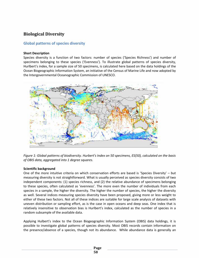
Page 58

Biological Diversity

Global patterns of species diversity

Short Description Species diversity is a function of two factors: number of species (‘Species Richness’) and number of specimens belonging to these species (‘Evenness’). To illustrate global patterns of species diversity, Hurlbert’s index, for a sample size of 50 specimens, is calculated here based on the data holdings of the Ocean Biogeographic Information System, an initiative of the Census of Marine Life and now adopted by the Intergovernmental Oceanographic Commission of UNESCO.

Figure 1: Global patterns of biodiversity. Hurbert’s Index on 50 specimens, ES(50), calculated on the basis of OBIS data, aggregated into 1 degree squares. Scientific background One of the more intuitive criteria on which conservation efforts are based is ‘Species Diversity’ – but measuring diversity is not straightforward. What is usually perceived as species diversity consists of two independent components: (1) species richness, and (2) the relative abundance of specimens belonging to these species, often calculated as ‘evenness’. The more even the number of individuals from each species in a sample, the higher the diversity. The higher the number of species, the higher the diversity as well. Several indices measuring species diversity have been proposed, giving more or less weight to either of these two factors. Not all of these indices are suitable for large scale analysis of datasets with uneven distribution or sampling effort, as is the case in open oceans and deep seas. One index that is relatively insensitive to observation bias is Hurlbert’s index, calculated as the number of species in a random subsample of the available data. Applying Hulbert’s index to the Ocean Biogeographic Information System (OBIS) data holdings, it is possible to investigate global patterns of species diversity. Most OBIS records contain information on the presence/absence of a species, though not its abundance. While abundance data is generally an

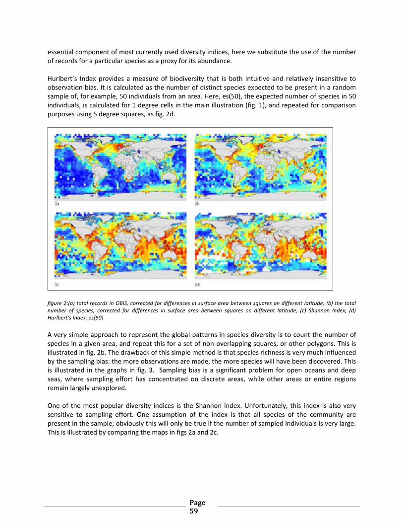
Page 59

essential component of most currently used diversity indices, here we substitute the use of the number of records for a particular species as a proxy for its abundance. Hurlbert’s Index provides a measure of biodiversity that is both intuitive and relatively insensitive to observation bias. It is calculated as the number of distinct species expected to be present in a random sample of, for example, 50 individuals from an area. Here, es(50), the expected number of species in 50 individuals, is calculated for 1 degree cells in the main illustration (fig. 1), and repeated for comparison purposes using 5 degree squares, as fig. 2d.

figure 2:(a) total records in OBIS, corrected for differences in surface area between squares on different latitude; (b) the total number of species, corrected for differences in surface area between squares on different latitude; (c) Shannon Index; (d) Hurlbert’s Index, es(50)

A very simple approach to represent the global patterns in species diversity is to count the number of species in a given area, and repeat this for a set of non-overlapping squares, or other polygons. This is illustrated in fig. 2b. The drawback of this simple method is that species richness is very much influenced by the sampling bias: the more observations are made, the more species will have been discovered. This is illustrated in the graphs in fig. 3. Sampling bias is a significant problem for open oceans and deep seas, where sampling effort has concentrated on discrete areas, while other areas or entire regions remain largely unexplored. One of the most popular diversity indices is the Shannon index. Unfortunately, this index is also very sensitive to sampling effort. One assumption of the index is that all species of the community are present in the sample; obviously this will only be true if the number of sampled individuals is very large. This is illustrated by comparing the maps in figs 2a and 2c.

Page 60

Sources of data Raw biogeographic data are available from many sources, such as large museums, national monitoring programmes, fisheries data, data from individual datasets, and so forth. The challenge is that these data are not always easily accessible, and that individual datasets are usually collected on a limited scope – geographic, taxonomic and temporal. The Ocean Biogeographic Information System (OBIS) was initiated to create a data warehouse to integrate this multitude of data in one comprehensive, quality-controlled system. OBIS is a work in progress, and increases steadily the quantity and quality of the data available through its portal. Its main contributors are

the field projects of the international Census of Marine Life

Regional OBIS Nodes, a network of often national organizations coordinating OBIS input for a region

thematic contributors such as OBIS SEAMAP (mammals, birds, turtles), MicrOBIS (microbes), FishBase or Hexacorallia

individual data holders such as the Smithsonian Museum, or the Continuous Plankton Recorder of the Sir Alister Hardy Foundation for Ocean Sciences

Important considerations Since species richness and evenness are independent factors, there is no unambiguous way to formulate the ultimate ‘diversity index’. Many indices have been proposed, often differing in the weight that is attached to either of the two components. Hill (1973) was able to show that many of the more commonly used indices are mathematically related. Several publications give a good overview of diversity indices, and their respective advantages and drawbacks (e.g. Magurran 1988; Grassle et al. 1979; Heip et al. 2001). Additionally, some measures also consider how different the species are from each other, such as how far they are separated on the “tree of life;” e.g. taxonomic distinctness (Warwick & Clarke, 1995; Clarke & Warwick, 1998). An assumption inherent in the approach of many diversity indices is that species are interchangeable – which obviously is not true. Diversity mainly consisting of invasive species is not a desirable situation; endangered and/or endemic species clearly should rank higher when making conservation decisions. So any final decision should take into consideration the actual species composition. Phylogenetic issues (i.e., issues pertaining to the evolutionary relatedness of species) have also been raised suggesting that it is better to have an area with species that are more distantly related than an area with only closely related species (e.g. Humphries et al. 1995). Indices that include relatedness exist (e.g. Warwick and Clarke, 1995, Clarke & Warwick, 1998), but require additional work before they can be calculated on large global data sets like OBIS. There are significant differences in the intensity with which the oceans are studied: many more data are available for coastal areas than for the open ocean. In the open ocean, surface waters are more intensively sampled than the bottom, and even fewer data are available for the mid-waters. Some large datasets (such as a long-line fisheries dataset from South Africa), with a massive number of records (more than 3 million) for very limited number of target species, results in low estimate of es(50) because the longline fisheries data can swamp the biodiversity analyses. For this reason, many practitioners turn to the use of species range maps when calculating species diversity indices. One example of such an approach is the Aquamaps model, which is discussed elsewhere in this document. Other models are,

Page 61

e.g., GARP (Stockwell and Peters, 1999) and WhyWhere (Stockwell 2006)15. Many of these tools are available through the OpenModeller web site (Muñoz et al. 2009)16. The content of OBIS, as it is now, is suitable for the study of broad patterns of the distribution of species diversity. The content is not sufficient to allow a detailed analysis on a regional scale, or to study the distribution patterns of individual taxa. But OBIS does provide a framework for capture and re-use of existing data, and will grow in time. It is a mechanism for data sharing, including data repatriation from the West to developing nations and small island states. The latter often do not have sufficient capacity to set up their own biodiversity data capture and management systems, and therefore could greatly benefit from global initiatives. CREDIT: E. Vanden Berghe, OBIS References Clarke KR, Warwick RM (1998) A taxonomic distinctness index and its statistical properties. J Appl Ecol 35:523–531 Grassle, J.F., Patil, G.P., Smith, W., Taille, C. (eds)(1979) Ecological diversity in theory and practice. Volume 6 in G.P. Patil (ed) Statistical Ecology. International C-operative Publishing House, Fairland, MD. xxi, 365 pp. Heip, C.H.R., Herman, P.M.J., Soetaert, K. (2001) Indices of diversity and evenness. Oceanis 24: 61-87. Hill, M.O. (1973) Diversity and evenness: a unifying notation and its consequences. Ecology 54: 427-431. Humpries, C.J., P.H. Williams, R.I. Vane-Wright (1995) Measuring biodiversity value for conservation. Annual review of Ecology and Systematics 26: 93-111. Hurlbert, S.H. (1971) The non-concept of species diversity: a critique and alternative parameters. Ecology 52: 577-586. Magurran, A.E. (1988) Ecological diversity and its measurement. Chapman & Hall. 179 pp. Muñoz, M.E.S., Giovanni, R., Siqueira, M.F., Sutton, T., Brewer, P., Pereira, R.S., Canhos, D.A.L. & Canhos, V.P. (2009) openModeller: a generic approach to species' potential distribution modelling. GeoInformatica. DOI: 10.1007/s10707-009-0090-7 Stockwell DRB. (2006) Improving ecological niche models by data mining large environmental datasets for surrogate models. Ecological Modelling 192(1-2):188-96. Stockwell, D. R. B., and D. P. Peters (1999) The GARP modelling system: Problems and solutions to automated spatial prediction. International Journal of Geographic Information Systems 13:143-158. Warwick, R.M. and K.R. Clarke (1995) New ‘biodiversity’ measures reveal a decrease in taxonomic distinctness with increasing stress. Marine Ecology Progress Series 129: 301-305.

15 available online at http://landshape.org/enm/whywhere-20-server-2/ 16 available online at http://openmodeller.sourceforge.net/

Page 62


Overlap between hotspots of marine mammal biodiversity and global seamount

distributions

Short Description AquaMaps is a species distribution model available as an online web service that generates standardized range maps and the relative probability of occurrence within that range for currently more than 9000 marine species from available point occurrences and other types of habitat usage information (Kaschner et al, 2006, Ready et al, accepted). By overlaying AquaMaps predictions for a subset of individual species (namely 115 marine mammals), we produced a global map of biodiversity patterns that shows the co-occurrence of predicted hotspots of marine mammal species richness and off-shore seamounts.

0.00

0.05

0.10

0.15

0.20

0.25

0.30

0 5 10 15 20 25 30 35 40

Species richness category

Mean

seam

ou

nt

den

sit

y

Figure 1(a) Global map of predicted marine mammal species richness and seamount density and 1(b) the highly significant

relationship between the two, spearman’s rho = 0.76, p < 0.0001) (both graphs modified from Kaschner, 2007)

Scientific Background

Species are not uniformly distributed on Earth. Heterogeneous physical features and community evolution drive the mix of species found in a given location. Places with high species diversity tend to contain greater genetic diversity and variety of physical habitats, as well as exhibiting greater resilience to environmental changes. Biological diversity, most commonly measured as the number of species present or species richness (versus number of genes or ecological habitats), provides an important composite measure of biological and ecological importance. Areas of high biological diversity, depending on their size and accessibility, may be identified either directly from intensive sampling or survey efforts. Alternatively, such hotspots of species richness may be inferred using habitat prediction models by overlaying a large number of predicted species occurrence data layers in a Geographic Information System (GIS) which will highlight areas of high co-occurrence of species. The vastness of the offshore marine environment and the resulting paucity of data for the open ocean or deep sea will likely preclude the identification of most areas of high biological diversity in the high seas through direct survey efforts alone in the foreseeable future. Thus large-scale species distribution models represent a useful alternative to evaluate the biological or ecological significance of an area

4

8

12

16

20

24

28

32

36

%%%%%%%%%%46

4

8

12

16

20

24

28

32

36

%%%%%%%%%%46

# of species 1a 1b

Page 63

based on this criterion by making inferences from better studied areas to those comparatively less well known (Wood et al, in review). In general, just as the physical environment often determines the limits of a single species’ distribution, high diversity in habitat can be a good predictor for species richness. In this example, high marine mammal species richness is predicted to correlate with greater seamount density. Seamounts aggregate prey and provide a wide range of environmental gradients for multiple species to thrive, often with enough physical separation to support diverging evolutionary histories. Here we see this diversity effect cascading all the way to top predators, i.e. marine mammals. How the areas of high biological diversity were identified

We used AquaMaps, an environmental envelope model which is a modified version of the relative environmental suitability model (RES) developed by (Kaschner et al. 2006) to visualize and investigate patterns of species richness. AquaMaps is available online and has been used to produce standardized range maps of > 9000 marine species to date. Predictions are provided in the form of relative probabilities of a given species to occur in each grid cell of a global grid of 0.5 degree latitude by 0.5 degree longitude cell dimensions. Using the tools available on the project web site, we selected and superimposed predictions for a subset of species, namely 115 marine mammals to visualize global patterns of biological diversity for these taxa. For each species, we assumed a relative probability threshold of 0.4 to define species presence in a given area. We then compared predicted marine mammal species richness in relation to a global seamount data set (Kitchingman et al, 2007) and found a significant relationship between areas of high marine mammal diversity and areas of high seamount density (Kaschner 2007). This preliminary analysis provided support that offshore seamounts represent biologically significant areas even for highly mobile and transient species such as most marine mammals. There are a wide range of available habitat prediction models requiring different types of input data and all coming with their own set of assumptions (see (Elith et al. 2006; Guisan et al. 2006; Guisan & Zimmermann 2000; Redfern et al. 2006). All of these models can, in theory, be used to generate predictions about species occurrence which can then be applied to make inferences about areas of high biological diversity. Most of these models tend to be more sophisticated and flexible in their assumptions than the AquaMaps approach. However, performance of all models is limited by the quality of their input data sets (Lozier et al, 2009) and currently available point occurrence data sets for large scale range predictions are affected by a large number of biases (see below). AquaMaps was specifically developed to deal with these biases to the extent possible and has been shown to perform as well as or better than other habitat prediction models when faced with currently available suboptimal, patchy, large-scale data sets (Ready et al., accepted).

Sources of Data

There are two types of input data used to generate AquaMaps species predictions. Firstly, available point occurrence records for the respective species, used to calculate all environmental envelopes (except for depth preferences) are harvested (and continually updated) from online data repositories such as the Ocean Biogeographic Information System (OBIS), OBIS-SeaMap (a sub-node of OBIS dealing specifically with marine mammals, seabirds and sea turtles), or the Global Biodiversity Information Facility (GBIF). Such point data sets are compiled from a variety of different sources and are generally affected by a number of sampling biases including, but not limited to, non-representative coverage of habitats and species misidentifications. To correct for misidentifications or geographic misallocations of occurrence records, information about the general occurrence of species in different ocean basins is


http://seamap.env.duke.edu/

http://www.gbif.org/

Page 64

used as a filter to select “good” points. This information is harvested from existing online species databases such as FishBase and SeaLifeBase where it is provided in the form of FAO statistical area checklists and/or bounding boxes delineating the known maximum range extent boundaries for species as described in the scientific literature. The concentration of sampling efforts in continental shelf areas often results in a mis-representation of the true depth usage of species. To counteract this bias, AquaMaps relies on depth usage information taken from the literature, as encoded in online species databases. To enable further correction of known biases or to predict occurrence for species for which point records are currently lacking, AquaMaps explicitly allows for the incorporation of further or alternative input data in the form of expert knowledge about habitat usage. This type of information can be used to adjust both envelope settings as well as bounding box/FAO area definitions during an expert review process.

Important considerations

Large-scale species distribution models currently probably represent the best, if not only choice to identify potential areas of high biological diversity in most of the often data poor off-shore regions of the world’s oceans. However, the concentration of sampling effort in more accessible habitats, such as the continental shelf regions of the northern hemisphere also represents a great challenge for the application of any species distribution modeling technique and results of all models therefore need to viewed with some caution. Most commonly, species distribution models predict broad range extents that often do not consider seasonal movements of animals or subspecies level population structure, and may thus potentially overlook critical habitat needed during certain life stages or for maintaining subspecies level diversity. When simply adding up the number of species, other useful information can be missed. For a given species, we are often interested in attributes such as: abundance, genetic uniqueness, endemism, and endangered status. However, most models and subsequently diversity indices derived from such predictions do not consider relative or absolute abundances of individual species and are indifferent to species substitutions. Hence, mapping of biodiversity hotspots may not reliably pick up on areas important to species of special concern, such as endangered and/or extremely rare species, although it is possible species weights can be assigned to add up a relative diversity measure inclusive of some of these aspects. Despite these caveats, which affect most currently existing models, an exercise such as the one conducted here may provide a starting point for evaluating the significance of an area. As indicated above, the tools and features available on the AquaMaps website allow for the selection of different subsets of species based on a range of different conservation and management criteria. Currently, taxa such as ray-finned fish and elasmobranchs as well as marine mammals are either complete or comprehensively covered by Aquamaps (see Figure 2), but coverage is currently being expanded to invertebrate, algae and hexacoral taxa. The incorporated expert review process represents a Wiki approach that can greatly facilitate the review of existing data and resulting predictions through expert panels such as IUCN species working groups. However, to most reliably identify areas of high biological diversity, a range of different modeling techniques should ideally be applied to determine which regions are consistently – across all model outputs - predicted to represent hotspots. Model selection and spatial and temporal scales of the analysis should be based on data availability and the ecology and life history of the taxa in question and outputs should be validated with independent, effort-corrected survey data to the extent possible. Forward projections of changes in species distributions and related areas of high biodiversity under different climate change scenarios can help to identify those significant areas most likely to ensure long-term protection of high biological diversity.

http://www.fishbase.org/

http://www.sealifebase.org/

Page 65

CREDIT: Kaschner, K., J. Ready, E. Agbayani, P. Eastwood, T. Rees, K. Reyes, J. Rius & R. Froese

References

Elith, J., C. H. Graham, R. P. Anderson, M. Dudý´k, S. Ferrier, A. Guisan, R. J. Hijmans, F. Huettmann, J. R. Leathwick, A. Lehman, J. Li, L. G. Lohmann, B. A. Loiselle, G. Manion, C. Moritz, M. Nakamura, Y. Nakazawa, J. M. Overton, A. T. Peterson, S. J. Phillips, K. Richardson, R. Scachetti-Pereira, R. E. Schapire, J. Soberon, S. Williams, M. S. Wisz, and N. Zimmermann. 2006. Novel methods improve prediction of species’ distributions from occurrence data. Ecography 29:129-151.

Guisan, A., A. Lehman, S. Ferrier, M. Austin, J. M. Overton, R. Aspinall, and T. Hastie. 2006. Making better biogeographical predictions of species’ distributions. Journal of Applied Ecology 43:386-392.

Guisan, A., and N. Zimmermann. 2000. Predictive habitat distribution models in ecology. Ecological Modelling 135:147-186. Kaschner, K. 2007. Air-breathing visitors to seamounts. Section A: Marine mammals. Pages 230-238 in T. Pitcher, T. Morato, P. J.

B. Hart, M. R. Clark, N. Haggan, and R. S. Santos, editors. Seamounts: Ecology, Fisheries & Conservation. Kaschner, K., R. Watson, A. W. Trites, and D. Pauly. 2006. Mapping worldwide distributions of marine mammals using a Relative

Environmental Suitability (RES) model. Marine Ecology Progress Series 316:285-310. Kitchingman, A., S. Lai, T. Morato, and D. Pauly. 2007. How many seamounts are there and where are they located. Pages 26-40

in T. Pitcher, T. Morato, P. J. B. Hart, M. R. Clark, N. Haggan, and R. S. Santos, editors. Seamounts: Ecology, Fisheries & Conservation.

Lozier, J. D., P. Aniello, and M. J. Hickerson. 2009. Predicting the distribution of Sasquatch in western North America: anything

goes with ecological niche modelling. Journal of Biogeography 36:1623-1627.

Ready, J., K. Kaschner, A. B. South, P. D. Eastwood, T. Rees, J. Rius, E. Agbayanii, S. Kullander, and R. Froese. (accepted). Predicting the distributions of marine organisms at the global scale. Ecological Modelling.

Redfern, J. V., M. C. Ferguson, E. A. Becker, K. D. Hyrenbach, C. Good, Barlow J, K. Kaschner, M. F. Baumgartner, K. A. Forney, L. T. Ballance, P. Fauchald, P. Halpin, T. Hamazaki, A. J. Pershing, S. S. Qian, A. Read, S. B. Reilly, L. Torres, and F. Werner. 2006. Techniques for cetacean-habitat modeling. Marine Ecology Progress Series 310:271-295.

Wood, L. T. Fuller, W.W. Cheung, H. Fox, K. Kaschner, A. Kitchingman, R. Watson & D. Pauly (in review). Identification of global marine priority areas using systematic conservation planning: developing a framework to meet global marine protection targets. Conservation Letters

Figure 2.

Example of AquaMaps current coverage: Map of ray-finned fish species richness and hotspots of biodiversity for more

than 6000 species

Page 66


Prediction of Biodiversity – Richness and Evenness

Short Description Patterns in biodiversity can be illustrated by variation in the number of species (richness) and whether these species are evenly distributed or dominated by a minority (evenness). Combining these two properties of biodiversity leads to the identification of uncommon communities that are deserving of greater protection. In this application we use a statistically rigorous analysis of species ranks combined with physical samples to predict patterns in biodiversity through the physical space. This extends our information from known biological samples to the broader environment, with measured uncertainty.

Figure 1. A characterisation of predictions of fish and invertebrate communities from Western Australia created by identifying unique combinations of species richness and community evenness from Rank Abundance Distributions.

Scientific Background Rank Abundance Distributions (RADs) are a ubiquitous distribution found in all biological samples where species abundances are counted. They are an ordering of all species in the sample from the most abundant to the least abundant. RADs are excellent metrics of community structure. The utility of predictions from RADs stems from three properties. First, they are a pattern that can be generated from any sample of an assemblage, irrespective of the actual sampling methods. Second, RADs are not dependent on species' identities and assemblages containing widely disparate species can be compared, allowing analysis over ecologically diverse areas. Third, rare species are explicitly included in the formation of a RAD. This last property is attractive as most methods for dealing with multispecies assemblages either discard rare species or transform the data until rare and abundant species can be dealt with in a statistical context. RADs are a reordering of the data found in Species Abundance Distributions (McGill et al. 2007)

Page 67

Figure 2: Predicted patterns of species richness for invertebrates on the Western Australian shelf and slope. Predicted mean richness (a) and coefficient of variation (b) are shown.

The shape of the RAD is a representation of the allocation of resources within a sample of a community. Communities where species partition relatively evenly will have relatively similar abundances while species that dominate resource use will likewise dominate the community. Most metrics of biodiversity can be calculated from RAD's (eg Shannon or Simpson diversity). However, we derive just three that come naturally from the distribution, total abundance, species richness and community evenness. How the criterion was applied We have developed a method of predicting Rank Abundance Distributions from physical covariates (Foster and Dunstan 2009, Dunstan and Foster (in review)). We decompose the RAD into three components that can each be predicted separately, total abundance, species richness and relative abundance. Statistical models can be constructed for each of the components and a measure of community evenness can be derived from the relative abundances of the predictions. Appropriate measures of uncertainty can be calculated from the asymptotic distributions of the fitted models. Predictions of derived metrics total abundance, species richness and community evenness can be mapped into physical space. Predictions of the means and standard errors of each of the components can be calculated. We have created a R package to perform model fitting, diagnostics and prediction with a similar interface to the standard GLM/GAM functions in R. This is freely available to any appropriately skilled researcher. This is not an EBSA for a particular region but a method of evaluating an area based on the EBSA biodiversity criterion. By predicting RADs using physical covariates, unique combinations of total abundance, species richness and community evenness can be identified. Examining the bivariate density of richness and evenness spatially allows maps to be generated that identify the spatial position and extent of these regions. Not all combinations of richness and evenness will be equally common, and particularly rare combinations may require additional management.

Page 68

Figure 3: Predicted patterns of evenness for invertebrates on the Western Australian shelf and slope. Predicted mean evenness (a) and coefficient of variation (b) are shown. Evenness varied from very even communities at 0 (shaded blue) to very uneven communities at -1.4 (shaded red)

Sources of Data

RADs can be calculated and used to help evaluate the ecological or biological significance of an area from any appropriate data set. The method requires counts for each species in a sample and accurate taxonomic identification so that species can be identified. To fit the models, physical covariates are needed at the location the sample was taken from. Predictions can then be made from the fitted models using covariates in new locations. The maps presented show the characterisation of communities for benthic fish and invertebrates in the continental shelf and slope adjacent to Western Australia from 21oS to 36oS. Models were parameterised with oceanographic data from the CSIRO atlas of regional seas (http://www.marine.csiro.au/~dunn/cars2006). Models can be developed for any region with appropriate biological data and covariates. It is not necessary for covariates to be measurements of physical processes, biologically derived covariates may be used (eg Organic Carbon). The only requirement is that biological covariates are collocated for model fitting and that the same covariates are available where predictions are being made.

Important Considerations

While RADs have been an acknowledged pattern in all sampled systems, understanding of their genesis and the ability to predict the distributions has been absent. Here we have used a statistical method to analyse and predict RADs to form measures of biodiversity for a wide range of habitats. The ability to combine and predict attributes of RADs into areas where sampling has not occurred will enhance both the management and understanding of the systems. The predicted patterns complement current understanding of the processes structuring deep sea benthic communities (Levin 2001). Our predictions show that processes acting at medium to large scales (e.g. temperature, salinity and oxygen concentrations) affect the structure of benthic assemblages. Even

http://www.marine.csiro.au/~dunn/cars2006

Page 69

though depth and latitude are useful surrogates to describe the patterns predicted here, they are not the covariates that structure most of the predictions. Rather it is other covariates such as temperature, salinity and oxygen that are important. This suggests that a simple interpretation using only depth and latitude would have missed important patterns that have emerged from our analysis. A deeper understanding of the patterns of biodiversity is obtained using a wide range of covariates that covers the range of environmental habitats. CREDIT: Piers Dunstan, CSIRO

References

Foster, S.D. and P.K. Dunstan 2009. The Analysis of Biodiversity Using Rank Abundance Distributions. Biometrics. DOI: 10.1111/j.1541-0420.2009.01263.x Dunstan, P.K. and S.D. Foster (in Review). RAD Biodiversity: Prediction of Rank Abundance Distributions from Deep Water Benthic Assemblages. Journal of Biogeography Levin, L., R. Etter, M. Rex, A. Gooday, C. Smith, J. Pineda, C. Stuart, R. Hessler, and D. Pawson. 2001. Environmental influences on regional deep-sea species diversity. Annual Review of Ecology and Systematics 32:51–93. McGill, B. J., R. S. Etienne, J. S. Gray, D. Alonso, M. J. Anderson, H. K. Benecha, M. Dornelas, B. J. Enquist, J. L. Green, F. He, A. H. Hurlbert, A. E. Magurran, P. A. Marquet, B. A. Maruer, A. Ostling, C. U. Soykan, K. I. Ugland, and E. P. White. 2007. Species Abundance Distributions: Moving Beyond Single Prediction Theories to Integration Within an Ecological Framework. Ecology Letters 10: 995–1015.

Page 70

Naturalness

South East Atlantic Seamounts

Short Description Global datasets of predicted large seamount locations have been created from ocean bathymetry. These data were combined with historical catch data from seamount fisheries and other anthropogenic marine impacts to identify areas of low impact including the waters around the Discovery tablemount group in the South East Atlantic.

Scientific Background Seamounts have been characterized as oases of productivity and diversity in the deep sea that also influence the productivity of the water column above (White et al. 2007). Formed by tectonic and volcanic activity, seamounts may act to disrupt normal oceanographic conditions across the abyssal plain, leading to an increase in vertical mixing and circulation (Roden, 1987). Such mixing, coupled with their relative isolation, can encourage the development of productive and often unique ecosystems. While the idea that all seamounts are highly productive environments has come into question in recent scholarship (White et al. 2007), the existence of highly productive “seamount fisheries” confirms that this concept is valid in many areas. Beginning in the late 1960s, seamount fisheries have seen major expansions both in terms of fishing effort and their geographic range over time (Watson et al. 2007). However, many seamounts are uncatalogued scientifically and untouched by fishing gears. As fishing is the single largest human disruption affecting most seamounts, a comparison of reported seamount fishing effort, known seamount locations, and their proximity to other anthropogenic impacts can inform the evaluation of the “naturalness” of a given seamount or seamount group.

Page 71

This illustration shows it is possible to identify seamounts in areas with low anthropogenic impacts using available global datasets. In a given biological province/region, less impacted seamounts can serve as a reference baseline. Such a reference baseline is crucial to quantifying anthropogenic impacts elsewhere and to evaluate seamount fishery management options. How the criterion was applied The naturalness criterion seeks to identify areas in the global ocean that have very low or absent levels of anthropogenic impact. Here, two datasets are used to estimate the naturalness of areas around seamounts: a global dataset of historical seamount catch (Clark et al. 2007) and a global model of human impacts (shipping, pollution, climate change etc) across as range of marine domains (Halpern et al. 2008). A global dataset of predicted seamount locations was obtained (Kitchingman & Lai 2004) (More information on these datasets is provided below). These data were imported into a Geographic Information System (GIS) and then combined based on location, with a historical seamount fishing effort dataset obtained from the Census of Marine Life project on Seamounts (CenSEAM) (Clark et al. 2007). This fishing effort dataset represents seamount-only catch volume in 1-degree cells. Since it is possible that several seamounts could exist in any cell, a count of seamounts in each fishing catch cell was performed and used to equally apportion the catch figures over the number of proximate seamounts. In addition, a global model of anthropogenic impacts across a range of marine domains was obtained (Halpern et al. 2008). These data were also combined, based on location, with the seamounts dataset. This combined dataset thus contained several metrics of surrounding anthropogenic impacts at each predicted seamount location. An initial filtering of the seamounts dataset to only those with summits < 2000m deep was performed (2000m being a current depth limit of existing fishing technology). Remaining seamounts were then identified in areas where seamount catch was known, and was less than 50 tons, and had a “Very Low” to “Low” impact score from the Halpern model. Once selected, the seamounts with the lowest impact score from Halpern were explored through existing literature. Only a handful of seamounts met all of these criteria, including seamounts in the Discovery tablemount group in the South East Atlantic off the west coast of South Africa. Seamounts in this group range from having no catch data reported (perhaps never fished, perhaps catch just not reported) to very little catch (<25 tons). There are no commercial fisheries currently established with most exploratory trawling taking place in the late 1970s and early 1980s (Clark et al. 2007). The Discovery seamounts have also been identified by the South East Atlantic Fisheries Organization (SEAFO) as “unexploited” and were closed to bottom fishing in 2006 (Bensch et al. 2008). In addition, an initial scientific sampling of these seamounts has been performed (Stocks 2009). A region of interest was drawn around the Discovery tablemount group and identified as a potentially ecologically significant area illustrating the naturalness criterion for seamounts. Sources of Data For this illustration we used seamounts data from a predicted seamounts dataset by Kitchingman and Lai (2004). This dataset is derived from global bathymetry data itself derived from soundings, sonar observations, and satellite altimetry data. Over 14,000 large (>1km in height) predicted seamounts are contained in this database (see http://seaaroundus.org/ecosystemsmaps/default.aspx to download these data). This number is thought to be a conservative estimate with some other estimates of global seamount counts ranging upwards of 100,000 (Wessel 2001)

http://seaaroundus.org/ecosystemsmaps/default.aspx

Page 72

These data were supplemented by historical global seamount catch data compiled by CenSEAM (Clark et al. 2007). Although these data are known to be incomplete, they represent the most comprehensive data for seamount fisheries to date and provided a reasonable indication of seamount trawl catch levels. Because these data are incomplete, only those cells with catch data were initially considered in this analysis. Cells with no data reported may have had no catch or may just be missing catch data. This biases the selection towards lightly impacted seamounts rather than undisturbed seamounts. However, the region of interest contains both seamounts for which catch is reported and seamounts for which no data are reported. This combination relies upon the best available data while hedging against the possibility that no data areas actually represented undisturbed seamounts. In addition a global model of anthropogenic impact on the global ocean was obtained (Halpern et al. 2008). This model was derived from a variety of marine impact data layers and its inverse was used as an additional broad proxy for naturalness in the marine environment. Analysis of multiple datasets across a geographic range can be accomplished using a Geographic Information System (GIS). Such systems allow for the basic overlay and selection analyses represented within this illustration. Using this methodology, additional datasets describing anthropogenic impacts or fishing effort could be added easily and more elaborate filtering and sub-selection performed. Important Considerations Concurrent with scientific exploration, seamount fishery exploration began in the late 1960s and 70s, establishing seamounts as a target for many global fisheries (Clark et al. 2007). Prior to more stringent reporting requirements, few data were collected on these early fishing efforts. It is believed that underreporting of fishing effort on seamounts continues to be a problem today (Bensch et al. 2008). Because fishing exploration has exceeded scientific exploration, much of what is known about seamounts is collected concurrent with, or after, the beginning of these extraction impacts. Despite a spate of recent seamount exploration globally, most are virtually unexplored scientifically. Of the 14,000 mapped seamounts (with many more thought to exist globally) only 300-400 have been the target of scientific sampling efforts, with less than 100 considered intensively sampled (Clark et al. 2006). In such a situation, modeling and proxy efforts can be used to estimate naturalness, where it remains, across this sparsely sampled domain. A more complete classification system of seamounts would help extend what is known about seamounts into those areas where less is known, building a more robust baseline upon which to develop this criterion. The methodology used in this illustration is readily grasped and depends only on the co-location of predicted seamounts and global impact datasets at a coarse resolution. No explanation of impact processes is here included and this co-location is assumed to indicate a direct negative impact (or lack thereof) on proximate seamounts. Nonetheless, the location of seamounts, historical seamount catch data, and co-located marine impact modeling together can serve as an initial assessment of known anthropogenic seamount impacts using the best available global data. CREDIT: J. Cleary, Duke University Marine Geospatial Ecology Lab, A. Rowden, M. Clark, & M. Consalvey, New Zealand National Institute of Water and Atmosphere andCenSEAM.

Page 73

References Bensch, A., M. Gianni, D. Gréboval, J.S. Sanders, and A. Hjort. 2008. Worldwide review of bottom fisheries in the high seas. FAO Fisheries and Aquaculture Technical Paper No. 522. FAO, Rome. Clark, M.R., V.I. Vinnichenko, J. Gordon, G. Beck-Bulat, N. Kukharev, and A Kakora. 2007. Large-scale distant-water trawl fisheries on seamounts. Pages 361-399 in T.J. Pitcher, et al., editors. Seamounts: Ecology, Fisheries & Conservation. Fish and Aquatic Resources Series, 12. Blackwell Publishing, Oxford, United Kingdom. Clark, M.R., D. Tittensor, A.D. Rogers, P. Brewin, T. Schlacher, A. Rowden, K. Stocks and M. Consalvey. 2006. Seamounts, deep-sea corals and fisheries: vulnerability of deep-sea corals to fishing on seamounts beyond areas of national jurisdiction. United Nations Environment Programme (UNEP) World Conservation Monitoring Centre (WCMC), Cambridge, United Kingdom. Halpern, B.S. et al., 2008. A Global Map of Human Impact on Marine Ecosystems: Science 319(5865), 948-952. Kitchingman, A., and S. Lai. 2004. Inferences on Potential Seamount Locations from Mid-Resolution Bathymetric Data. Pages 7-12 in T. Morato and D. Pauly, editors. Seamounts: Biodiversity and Fisheries. Fisheries Centre Research Reports. University of British Columbia, Vancouver, Canada. Kitchingman, A., S. Lai, T. Morato, and D. Pauly. 2007. How many seamounts are there and where are they located? Pages 26-40 in T.J. Pitcher, et al., editors. Seamounts: Ecology, Fisheries & Conservation. Fish and Aquatic Resources Series, 12. Blackwell Publishing, Oxford, United Kingdom. Roden, G.I., 1987. Effects of seamounts and seamount chains on ocean circulation and thermohaline structure. Pages 335-354 in B.H. Keating et al., editors. Seamounts, Islands, and Atolls, Geophysical Monograph Series, Vol XXXXIII. AGU, Washington, D.C. Stocks, K. 2009. SeamountsOnline: an online information system for seamount biology. Version 2009-1. World Wide Web electronic publication. http://seamounts.sdsc.edu. Wessel, P. 2001. Global distribution of seamounts inferred from gridded Geosat/ERS-1 altimetry: Journal Of Geophysical Research-Solid Earth 106(B9), 19431-19441. Watson, R., A. Kitchingman, and W. Cheung. 2007. Catches from world seamount fisheries. Pages 400-412 in T.J. Pitcher, et al., editors. Seamounts: Ecology, Fisheries & Conservation. Fish and Aquatic Resources Series, 12. Blackwell Publishing, Oxford, United Kingdom. White, M., I. Bashmachnikov, J. Arístegui, and A.R. Martins. 2007. Physical processes and seamount productivity. Pages 65-84 in T.J. Pitcher, et al., editors. Seamounts: Ecology, Fisheries & Conservation. Fish and Aquatic Resources Series, 12. Blackwell Publishing, Oxford, United Kingdom.

Documents

Defining ecologically or biologically significant … ecologically or biologically significant areas in the open oceans and deep seas: Analysis, tools, resources and illustrations