AD-A281 668\u1,.!'I',I ll ~'lh| 1' \1• I' Ill,

Defense Nuclear Agency IAlexandria, VA 22310-3398

DNA-TR-93-63

Laboratory Investigation and Analysis of theStrength and Deformation of Joints andFluid Flow in Salem Limestone - DTIC

&!AELFCTEDaniel E. Cohitty, et a!. JUL 17 ,

Applied Research Associates, Inc.New England DivisionRFD #1 Box 120AWaterman RoadSouth Royalton, VT 05068

June 1994

Technical Report

CONTRACT No. DNA 001 -90-C-01 32

Approved for public release;

94 22176 \distribution is unlimited.

94 7 14 062

BestAvailable

Copy

Destroy this report when it is no !onger needed. Do notreturn to sender.

PLEASE NOTIFY THE DEFENSE NUCLEAR AGENCY,

ATTN CS1I, 6801 TELEGRAPH ROAD, ALEXANDRIA, VA22310-3398, IF YOUR ADDRESS IS INCORRECT, IF YOUWISH IT DELETED FROM THE DISTRIBUTION LIST, ORIF THE ADDRESSEE IS NO LONGER EMPLOYED BY YOUR

ORGANIZATION.

O Pj' *

Ai ,,l

DISTRIBUTION LIST UPDATE

This mailer is provided to enable DNA to maintain current distribution lists for reports. (We wouldappreciate your providing the requested information.)

NOTE:0 Add the individual listed to your distribution list Please return th oiailing label from

the documt at any additions,0 Delete the cited organization/individual. changes, corlb-,wrns or deletions can

be made easily.

O Change of address.

NAME

ORGANIZATION:

OLD ADDRESS CURRENT ADDRESS

z TELEPHONE NUMBER: ( )ZI

SDNA PUBLICATION NUMBER/TITLE CHANGES/DELETIONS/ADDITIONS, etc.)0 (Artech Se• , if moe Spec* in Required)

<c

WIIuJ"i-a

S DNA OR OTHER GOVERNMENT CONTRACT NUMBER:

CERTIFICATION Or NEED-TO-KNOW BY GOVERNMENT SPONSOR (if other than DNA):

SPONSORING ORGANIZATION:

CONTRACTING OFFICER OR REPRESENTATIVE:-

SIGNATURE:

DEFENSE NUCLEAR AGENCYAT'TN: TITL6801 TELEGRAPH ROADALEXANDRIA, VA 22310-3398

DEFENSE NUCLEAR AGENCYATTN: TITL6801 TELEGRAPH ROADALEXANDRIA. VA 22310-3398

REPORT DOCUMENTATION PAGE FO,,A4 No. 04- F8

"'A.ia wror"N b.r~o for thecwet so .Coa' --a r * on~st. * aa.,.ae to 9e i t~ 94ý aOW ~ ) 1016n 1-fm e ? 1 to a-e~ng irwrýe.,a tt,.~ e.w-9 data SO7,oc,1mWW.. W" nt'.tngMO dmt now"'L 4-- -,mý..t a&M fe..aN~n me4 ~i~T of i nfow.,o, Send c-mi.nn egbonmg ",, b,,o'da. w t, a n, *1ttat asoect of IOWdaSnti~ O1 ýttq-s~vton nW,0nq *V9991100 o r',I redtýV tht rI, , btda to W.Ittt(,o. Nsaqa~,rtrWV Semo,. ),& c~r ~ n ,tao, , o0u,ot,, and .o A000 1215 ýrweýo~Da"s. HqlFt4,. S..t. 1204. Al-,twon VA 22202-4302 wW t€o me Ofe 0A ..4ana n.,t e•,and Bfa.i Pft ,,won, Rea& t'-,o, Pm•4v. 10704-01t , wa.•', oe. DC 20WSW1. AGENCY USE ONLY (Leave b/en;,T 2 REPORT DATE 3. REPOR" iTYPE AND DATES COVERED

940001 Technical 900801 - 930630

4 TITLE AND SUBTITLE 5. FUNDING NUMBERS

Laboratory Investigation and Analysis of the Strength and C - DNA 001-90-C-0132Deformation of Joints and Fluid Flow in Salem Limestone PE - 62715H

•PR - RS6. AUTHOR(S) PR - RSTA - RHDaniel E. Chitty, Scott E. Blouin, Xiaoqing Sun, and - DH303150Kwang J. Kim

7. PERFORMING ORGANIZATION NAME(S) AND ADDRESS(ES) 8. PERFORMING CRGANIZATIONApplied Research Associates, Inc. REPORT NUMBERNew England DivisionR]D #I1 Box 120A 5634Waterman RoadSouth Rovaltun, VT 05068

9 SPONSORING/MONITORING AGENCY NAME(S) AND ADDRESS(ES) 10. SPONSORING/MONITORINGDefense Nuclear Agency AGENCY REPORT NUMBER6801 Telegraph RoadAlexandria, VA 22310-3398 DNA-TR-93-63SPSD/Senseny

I 1. SUPPLEMENTARY NOTES

This work was sponsored by the Defense Nuclear Agency under RDT&E RMC CodeB4662D RS RH 00018 SPSD 4300A 25904D.

12a. DISTRIBUTION/AVAILABILI"Y STA1 EMENT 12b. "ISTRiBUTION CODE

Approved for public release; distribution is unlimited.

13. ABSTRACT (Marini m 200 words)As part of the Underground Technology Program, fundamental mechanisms that influencethe mechanical response of jointed, saturated rock masses were investigated withlaboratory tests performed on Salem (Indiana) limestone. Mating joint surfaces werecreated by 1) tensile splitting, 2) sawing and grinding, and 3) cutting to aspecified fracta.l dimension using numerically controlled machine tools. Triaxialtests on specimens with inclined joints were performed to measure joint strengthand deformation, and a constitutive model for joints was developed, including theobserved strain softening. Permeability of the intact limestone was measured atvarious stress states including deviator stresses, and joint flow was measured undera range of normal stress conditions. Other dspects of the project included aninvestigation of strain rate effects, and measurement of the saturated undrainedcompressibility and specific storage of the limestone.

This contract also sponsored ARA's participation in an interlaboratory test programsponsored by the Institute for Standards Research of the American Society for Testingand Materials to develop statements of precision and bias for four standard rocktest methods.14. SUBJECT TERMS 15. NUMBER OF PAGES

Rock Mechanics Fractais Limestone 378Rock Joints Constitutive Modeling Permeabilitv 16. PRICE'CODE

17 SECURITY CLASSIFICATION 18. SECURITY CLASSIFICATION 19 SECURITY CLASSIFICATION 20. LIMITATION OFOF REPORT OF THIS PAGE OF ABSTRACT ABSTRACT

UNCLASSIFIED UNCLASSIFIED UNCLASSIFIED SAR4SN 7540-01-280-5500 i Sianc,"rd Form 298 (Rev 2-89

P'ePcimbed by ANSI Sts 239 18

298 -02

UNCLASSIFIEDSECURMY CLSS;.'CAT1ON OF TMIS PAGE

CLASSIFIED BY.

N/A since unclassified.

DECLASSIFY ONN/A sinc- Unclassified.

Aoce>i- to-

(l l• k' A •i

U;;l;ic l

ByJ,• t :.... ; 't ',u,

SECURITY CLASSIFICATION OF THIS PACE

UNCLASSIFIEDi-i

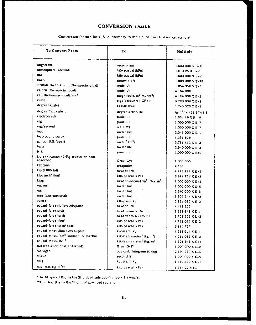
CONVERSION TABLE

Conversion factors for U.S. customary" to metric (SI) units of measurement

To Convert From To Multiply

angstrom meters (ml 1.000 OO0 X E--I0atmosphere (normal) kilo pascai (kPa) 1.013 25 X E.2bar kilo pascal (kPal 1.000 000 X E+2barn meter 2 (M2) 1.000 000 X E-28British Thermal unit (thermochemlcall joule (JI 1.054 350 X E ý3calorie (thermochbemical) Joule IJ) 4.184 000cal (thermochemicall/cm 2

mega joule/m 2 [MJ/m 2) 4.184 000 X F-2curie giga becquerel iGBqlJ 3.700 000 X E+ Idegree (anglel rad'an (radl 1.745 329 X E-2

degree ,hrenheit degree kclvin IK) tx=tLof + 459.67).' 1.8electron volt Joule (J) 1.602 19 X F_ 19erg joule (JI 1.000 000 X E-7erg!second watt (W) 1.000 000 X E-7foot meter (m) 3.048 000 X E--Ifoot-pound-force Joule (J) 1.355 818gallon (U.S. liquid) meter 3

(m3 ) 3.785 412 X E-3inch meter (m) 2.540 000 X E-2je• k joule iJi I L 0A x EA L-"

Joule/ kilograrn W/Kg) (radiation doseabsorbed) Gray iGy) 1.000 000kilotons teraJoules 4.183kip (1000 lbfl newton (N) 4.448 222 X E+3kip/Lnch 2 iksl) kilo pascal (kPa) 6.894 757 X E+3ktap newton-second/rm 2 (N.-s/n 2 ) 1 .0O0 000 X E+2micron meter 1m) 1.000 000 X E-.6mil meter Im) 2.540 000 X E-5mile (International) meter 1m) 1.609 344 X E+3ounce kilogram (kg) 2.834 952 X E-2pound-fuoce )!bf avoirdupois) newton (N) 4.448 222pound-force Inch newton-meter (N-m) 1.129 848 X E-lpound-force/inch newon/meter IN/m]1 1.751 268 X L+2pound-force/foot 2

kilo pascal (kPa) 4.788 026 X E-2pound-force/Inch 2 (psi) kilo pascal (kPa) 6.894 757pound-mass (Ibm avoirdupois) kilogram (kg) 4.535 924 X E--Ipound--mass--foot 2 (moment of Inertia) kilogram-meter2 (kgm2 ) 4.214 011 X E-2pound-massifoo°t kilogram!meter3 (kg/ri') 1.601 846 X E+Irad (radiation dose absorbed) Gray (Gy)" 1.000 000 X E-2roentgen coulomb;kilogram (C/kg) 2.579 760 X E-4shake second (9s 1 .000 000 X E-6slug ktlrgrarn (kg) 1.459 390 X E+ Itorr (mm Hg. 0 C) kilo pascal IkPa) 1 333 22 X E,-]

'The becquerel (Bq) is the Sl unit of radl'.actvlty: Bp - I eventis."The Gray (Gy) is the SI unit of ab.Lo aed radiation.

Illw,

LM7

TABLE OF CONTENTS

Section Page

CONV ERSIO N TABLE .................................................. ii

F IG U R E S . . . . . . . . . . . . . . . . . . . . . .. . . . . . . . . . . . . . . . . . . . . ii

T A B L E S . . . . . . . . . . . . . . . . . . . . . . . . . . . . . . . . . . . . . . . . . . . . xv i

1 IN TROD U CTIO N .....................................1.1 BAC KGRO U ND .. ................................... 11.2 OBJE C TIV ES . . .... . .. . . . . .. .. . ... ... . . .. . . . . .. . . .1.3 SC O P E . . . . . . . . . . . . . . . . . . . . . . . . . . . . . . . . . . . . . .. . . 2

2 SALEM LIMESTONE ORIGIN, DESCRIPTION. AND PHYSICALPR O PER TIES . .. . . . . . . . . . . . . . . . . . . . . . . . . . . . . . . . . . . . . . 42.1 OPJGIN AND DESCRIPTION . .......................... 42.2 PHYSICAL PROPERTIES . ............................. 5

3 JOINT SURFACE PREPARATION ........................... 83.1 JOINT SURFACE FABRICATION ........................ 8

3.1.1 Smooth Ground Joint Surfaces ....................... 83.1.2 Tensile Fracture Joint Surfaces ....................... 93.1.3 Synthetic Joint Surfaces ....... ................... 9

3.2 SURFACE GEOMETRY MEASUREMENT .................. 11

4 TEST PROCEDURES ................................... 214.1 SPECIMEN PREPARATION .1........................... 14.2 MOISTURE CONTENT PREPARA7ION . ................... 22

4.2.1 Unsaturated Specim ens . ....................... ... 224.2.2 Saturated Specim ens . .. ..... ..................... 22

4 .3 LO A D IN G . . . . . . . . . . . . . . . . . . . . . . . . . . . . . . . . . . . . . . . . 234.3.1 Triaxial Com pression . ............ ............... 234.3.2 Hydrostatic Compression ............................ .44.3 3 Uniaxial Strain . . .. . .... . . . . . .. ... . . . . . . . . . ... . . 24

4.4 INSTRUM ENTATION ................................. 244.5 DATA RECORDING AND REDUCTION ........ .......... 25

5 MECHANICAL PROPERTIES OF INTACT LIMESTONE .............. 305.1 UNCONFINED COMPRESSION TESTS ..................... 31

5.1.1 Unconfined Compression Tests at Various Water Contenws ...... .315.1.2 Post-Failure Response ot Limestone in Unconfined Compression. 32 ...

5.2 TRIAXIAL COMPRESSION TESTS ........................ 335.2.1 Intact Strength Determination .. ....................... 145.2.2 Investigation of Specimen Aspect Ratio and End Conditions ...... .34

5.3 HYDROSTATIC COMPRESSION TESTS ...................... 375.5 UNIAXIAL STRAIN TESTS . ..... .. .. . ...... 38

iv,

TABLE OF CONTENTS (Continued)

Section Page

6 MECHANICAL PROPERTY TESTS ON JOINTED LIMESTONES PE C IM E N S . . . . . . . . . . .. . . . . . . . . . . . . . . . . . . . . . . . . . . . 586.1 TEST PROCEDURES . ................... ............ 586.2 STRENGTH TEST RESULTS ................ .......... 596.3 JOINT DEFORM ATION ............................... 63

7 EFFECTS OF VARIATIONS IN DEFORMATION RATE ... ....... S37.1 STRAIN RATE TESTS ON INTACT SALEM LIMESTONE ........ 83

7. 1. 1 Numerical Simulauons of Intact Tests .................... .,847.2 STRAIN RATE TESTS ON JOINTED SALEM LIMESTONE ........ 86

8 SATURATED UNDRAINED HYDROS-ATIC COMPRESSION TEST ANDSPECIFIC STORAGE MEASUREMENT ....................... 1038.1 TEST PROCEDURES ................................. 1038.2 T"EST RESULTS ....... ............................. .. (48.3 RATIO BETWEEN PORE PRESSURE AND HYDROSTATIC STRESS - 1048.4 SPECIFIC STORAGE ..................... ........... 106

0r fhD Afl tbYT T r' f-%r i'- .'- Tl -. -

9 . -r 1-" \ " '1 r 0-,,- IN ACT IAN JOINTED LiMESTOINE .......... 116

9.1 DESCRIPTION OF EXPERIMENT. ....................... 1169.1.1 Test Specimens. Equipment. and Instrumentation ............. 1179.1.2 Test Procedures . .. . . . . . . . . . . . . .. . .. . . . . . .. . . . . . . 1189.j.3 t-iu i-low Lqua ions .. ............................ 119

9.2 PERMEABILITY OF INTACT SALEM LIMESTONE ............ 1229.2.1 FlowA Tests with Hydrostatic Skeleton Loading .............. 1229.2.2 Flow Tests with Triaxial Skeleton Loading ............... .. 124

9.3 PERMEABILITY OF JOINTED SALEM LIMESTONE SPECIMENS . .. 125

9.3.1 Joint Permeability Formulations . ...................... 1269.3.2 Tensile Fracture Joint Permeability Test ResulLs ............. 127,9.3.3 Smooth Ground Joint Permeability Test Results ............. 1329.3.4 Synthetic Joint Permeability Test Results ............. ... 133

10 NUMERICAL SIMULATION OF ROCK JOINT RESPONSE ........... 18110.1 THEORETICAL DERIVATION OF ELASTOPLASTIC RESPONSE OF

JO IN T S . . . . . . . . . . . . . . . . . . . . . . . . . . . . . . . . . . . . . . . 18 110 .1.1 N o tations . . . . . . . . . . . . . . . . . . . . . . . . . . . . . . . . . . . . 18 110.1.2 Total Strain Increm ent ............................ 18310.1.3 Elastic Stress-Strain Relationship ..................... 18310.1.4 Y ield Eq uation . . . . . .. . . . . . . . . . . . . . . . . . . . . . . . . . . 18410.1.5 F low R ule . . . . . . . . . . .... . . . . . . . . . . . . . . . . . . . . . . 18510.1.6 Norm al to the Yield Function ............. .......... 18610.1.7 C onsistency Equation ..... ............... . ... ..... I86

1. 1.8 Formulation of Eiastoplastic Stress-Strain Matrix ... .......... 17

v

TABLE OF CONTENTS W(ontinucd)

Section Page

10.2 IVALI.'AT'ION 01. MOI)EL PARAMTEI-RS FI)R TIINSILE-FRACTURE JOiNTS OF SALLM LIM:ISI:S )Ni ........ .... I

10-2.1 Elastic C onstanLs . . . .. . ... ... . . . . . . .. . I N9

10.2.2 Joint C om pres:;ibility . . . . . . . . . . . . . . . . . . . . . . . . . . . . . I N)

10.2.3 Peak and Residual Shear Strength Paranictcl ............... 1 110.2.4 Strain Softening Parameter ............................... 19210.2.5 Plastic Potential Parameters ............. .... ......... ...... 192

10.3 VERIFICATION PROBLEM ................................ 19310.4 CONCLUSIONS RELATED TO JOINT SIMULATION ........... 194

11 ASTM/ISR INTERLABORATORY TEST PROGRAM .................. 20711.1 SPECIMEN PREPARATION AND MEASUREMLNT .......... 207

11. 1. 1 Phase 1 Specimen Preparation .. .................... 20611. 1 .2 Phase 2 Specimen Preparation ..... ................... 208

11.2 ULTRASONIC WAVESPEED MEASUREMENTS ............. 20911.3 UNCONFINED COMPRESSION TESTS ................... .. 20911.4 SPLITTING TENSILE STRENGTH TESTS ................. 21011.5 TRIAXIAL COMPRESSION TESTS'S ..................... 210

12 SUMMARY AND CONCLUSIONS ..... .................. ... 22

13 REFERENC ES . . ... ... . ... .... ... .... .... .... ....... 232

Appendix Page

F ̀ 01, 1 EL OF JOINT SURFACES ........................ a,-

B UNCONFINED COMPRESSIVE TESTS WITH POST FAILURER E SPO N SE . . . . . . . . . . . . . . . . . . . . . . . . . . . . . . . . . . . . . . . . . B -I

C TRIAXIAL COMPRESSION TESTS ON INTACT SPECIMENS ......... C-1D HYDROSTATIC COMPRESSION TESTS ................ .... D-1E UNIAXIAL STRAIN TESTS ........................ ..... E- IF ASTM/ISR INTERLABORATORY COMPARISON TESS .............. F-I

Vi1

Figure Page

3-1 Phott'graphs of [htit 1hrc type,,s otit u la d e, used InI 1int tcstlilg .... .1

2 Layo ut Of the pio)1lliCnes Ito charact.ri/ation of joint surfaces on sheartest specimen"s ....... ...................................... 1 5

3-3 Typical projiles of a tensile fracrurc JO.101 .......................... 10

3-4 Typical profiles of a synthetic joril, ............................. 17

3-5 , FT aliphtudcs of thlIrc typ:cal tensile lfacture joint profiles ............ is

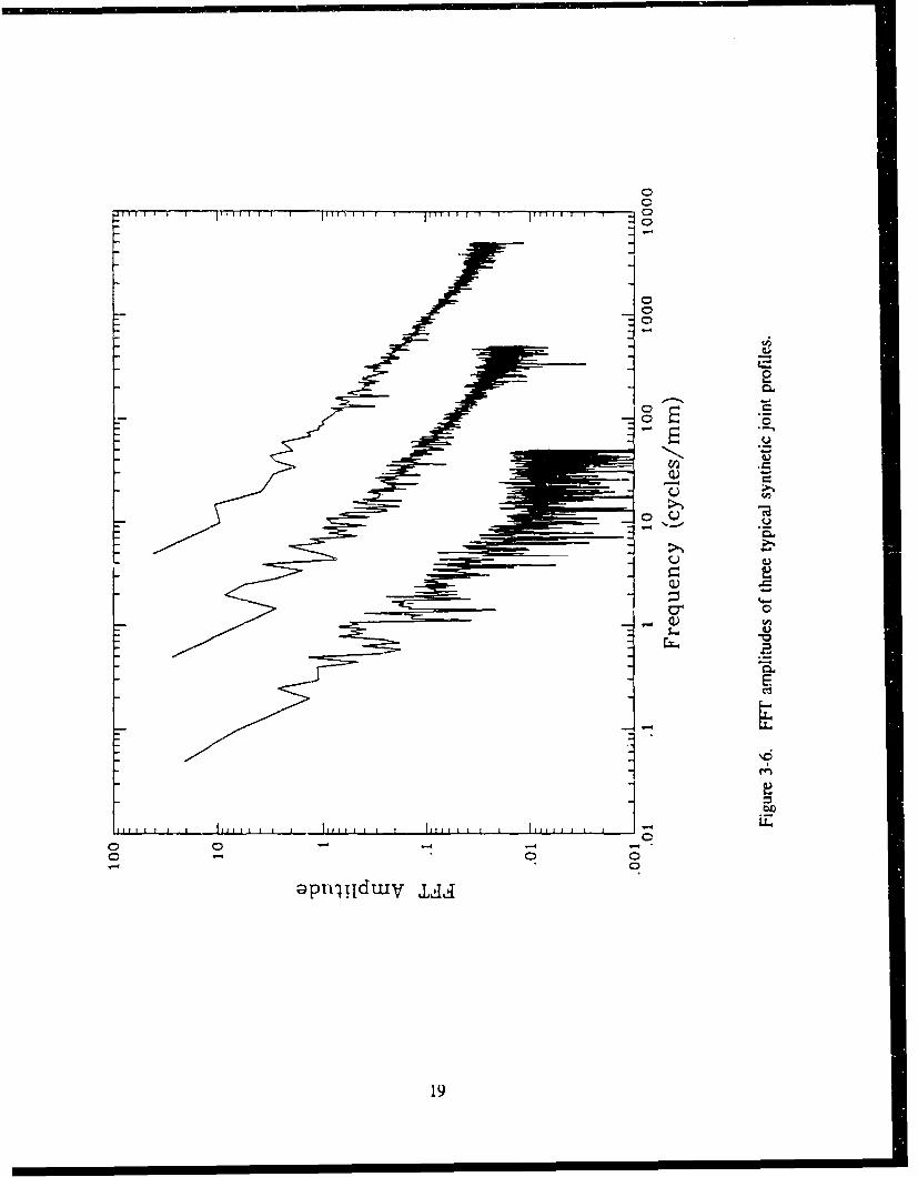
3-., FFT amplitudes of three typical syntheuc joint profiles ................. 19

3-7 Comparison of the average FFT amplitudes of ten profiles each on atonsile fracture joint and a synthetic joint ........................... 20

4- ChoL o, picparation and instrumentauton of triaxial spec:mens ..... 28

4-2 Schematic of system lot saturation of porous tnaxial test specimens ..... .. 29

5-1 Illustration of the relationship between water content and unconfinedstrengths in Salem limestone. .................................. .42

5-2 SchematL. of the stiffener ring used in tesLs to determine post-liiluieresponse of Salem limestone in unconfined compression ................ 43

53 Overlay of six axial stress-strain curves including post-failureresponsc of Salem limestone in unconfined compression ............... 44

5-4 Comparis i, of axial stres,;-strain curves for Salem lmestone tested intriaxial compression at a range 01 confining pressufe iii the brittie regime . 5

5-5 Strength data from trtaxial compression tests on intact Salemrlimnictone specimeos at .onlIining pressures ranging from zero to 4(X) MPa . 46

5-6 Strength data from triaxial conipression tests on intact Salemlimestone specimens at confining pressures ranging fioni icro to 25 MPa 47

5-' Comparison of pre-lailure response of Salem limestone tested intnaxial compression at 25 NI Pa confining pressure under three dillerenttest cond:tions ............................................

vi

FIGURES (Coutinued)

Figure Page

5-S Relationship between average axial strain and radial strains measured in a 25-IMIPa tnaxial compression test at threc different heights on a test specimen A ithLID = 2 and unlubricated ends ................................. .49

5-9 Relationship bctwccn average a- ial strain and radial strains n;easured in a 25-MPa triaxial compression test at three different heights on a test specimen withLID = 2 and lubncated ends ....... ........................... 50

5-I10 Relationship between average axial strain and radial strain measured in a 25-MPa tnaxial compression test on a test specimen with L/D = 1 and lubncatdends .......... ............................................ 51

5-1 1 Comparison of volumetric strains computed from 25-MPa triaxial compressionunder three different test conditions ............................... 52

Salem limestone loaded in hydrostatic comprcssion ................... 53

5-13 Typical relationship betv.een axial and radial strain for intact Salem limestoneloaded in hydrostatic compression ................................ 54

5-14 Typical relationship between axial stress and axial strain for intact Salemlimestone loaded in uniaxial strain ....... ......................... 55

5-15 Typical relationship between axial stress and confining pressure for intactSalem limestone loaded in uniaxial strain .......................... 56

5-16 Typical relationship between mean stress and volumetric (axial) strain forintact Salem limestone loaded in uni.xial strain ...................... 57

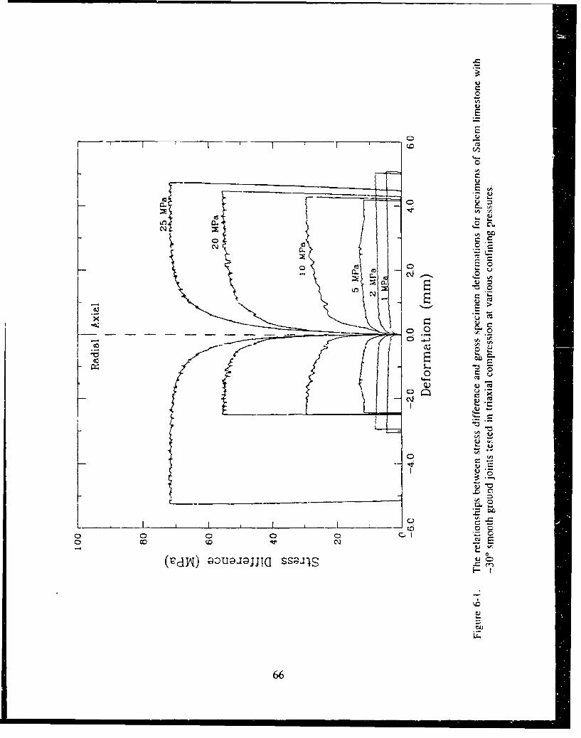
6-1 The relationships between stress difference and gross specimen deformationsfor specimens of Salem iimestone with - 30' smooth ground joints tested intriaxial compression at various confining p-essures ................... 6 6

6-2 The relationships between stress difterence and gross specimendeformations for specimens of Salem limestone wvith - 30 ' tensile Iraciurejoints tested in triaxial compression mt various confining pressures ...... .. 67

viii --

FIGURES (Continued)

Figure Page

6-3 The relationships between stress difference and gross specimendeformations for specimens of Salem limestone with - 30" syntheticjoints tested in triaxial compression at various confining pressures ...... .. 68

6-4 The relationships between stress difference and gross specimendeformations for specimens of Salem limestone, both intact and with threetypes of - 300 smooth ground joints, tested in triaxial compression at 1MPa confining pressure ...................................... 69

6-5 The relationships between stress difference and gross specimen deformationsfor specimens of Salem limiestone, both intact and with three types of - 30"smooth ground joints, tested in triaxial compres.;ion at 2 MPa confiningpressure ....... ......................................... 70

6-6 The relationships between stress difference and gross specimen deformationsfor specimens of Salem limestone, both intact and with three types of - 30'smooth ground .Joints, tested in triaxial compression at 5 MPa confiningpressure ........ ........................................ 7i

6-7 The relationships between stress difference and gross specimen deformationsfor specimens of Salem limestone, both intact and with three types of - 30')smooth ground joints, tested in triaxial compression at 10 MPa confiningpressure ....... ......................................... 7.

6-8 The relationships between stress difference and gross specimen deformationsfor specimaens of Salem limestone, both intact and with three types of -30"smooth ground joints, tested in triaxial compression at 20 MPa confiningpressure ....... ......................................... 73

6-9 The relationships between stress difference and gross specimen deformationsfor specimens of Salem limestone, both intact and with three types of - 30('smooth ground joints, tested in triaxial compression at 35 MPa confiningpressure ....... ......................................... 74

6-10 Peak strength data for three types of joints in Salem limestone with tiestrength envelope tor intact rock shown for comparison ................ 75

6-11 Residual strength data for three types of joints and intact Salem limestonewith the peak strength envelopes shown for comparison .... ............ 76

xi

FIGURES (Continued)

Figure Page

6-12 Normal and tangential deformations of smooth ground joints in Salemlimestone plotted against normal and tangential deformations, respectively,for a range of confining pressure conditions ....................... 77

6-13 Normal and tangential deformations of tensile fracture joints in Salemlimestone plotted against normal and tangential deformations, respectively,for a range of comining pressure conditions ....................... 78

6-14 Normal and tangential deformations of synthetic joints in Salemlimestone plotted against normal and tangential deformations, respectively,for a range of conf'iing pressure conditions ....................... 779

6-15 Relationship b-tween normal and tangential deformation of smooth groundjoints in Saleia limestone under a range of confining pressure conditions . . 80

6-16 Relationship between normial and tangential deformation of tensile fracturejoints in Salem limestone under a range of confining pressure conditions . . 81

6-17 Relationship between normal and tangential deformation of syntheticjoints in Salem limestone under a range of confining pressure conditions . . 82

7-1 Comparison of stress-strain curves from intact unsaturated (2-5% watercontent) Salem limestone specimens tested in triaxial compression with20 MPa confining pressure at strain rates of 10W, 10 ', and 10-3 s ...... .... 89

1

7-2 Comparison of stress-strain curves from intact saturated Salem limestonespecimens tested in drained triaxial compression with 20 MPa confiningpressure at strain rates of 10l' and 10' s ......................... 90

7-3 Comparison of stress-strain curves from intact unsaturated (2-5% watercontent) Salem limestone specimens tested in triaxial compression with25 MPa confining pressure at strain rates of 1W5, 10-4, 10-2. s ........ ... 91

7-4 Summary of the relationship between strength and strain rate for the test datapresented in Figure 7-1 through 7-3 ............................. 92

7-5 Comparison of mean stress-volume strain curves from intact unsaturated(2-5% water content) Salem limestone specimens tested in triaxialcompression with 20 MPa confining pi ssure a' strain rates of 10:

and 10' s* ................ ........................................ 93

x

FIGURES (Continued)

Figure Page

7-6 Illustration of the finite element mesh used to simulate the saturated drainedtests on intact limestone specimens .............................. 94

7-7 Mean stress and pore pressure as functions of volume strain from anumerical simulation of the saturated drained 20-MPa triaxial compressiontest at 10, s-1 strain rate, showing the measured mean stress forcomparison ....... ....................................... 95

7-8 Mean stress and pore pressure as functions of volume strain from anumerical simulation of dhe saturated drained 20-MPa triaxial compressiontest at 10-1 s- strain rate, showing the measured mean stress forcomparison ....... ....................................... 96

7-9 Comparison of stress-strain curves from 30' tensile fracture jointedSalem limestone specimens tested in triaxial compression with 20 MPaconmining pressure at strain rates of 101 and 10-3 st and different initialsaturation conditions ........................................ 97

7-10 Comparison of stress-strain curves from 30' smooth ground jointedSalem limestone specimens tested in triaxial compression with 20 MPaconfining pressure at strain rates of 10W and 10" s*' and different initialsaturation conditions ........................................ 98

7-11 Comparison of stress-strain curves from 30' synthetic jointed Salemlimestone specimens tested in triaxial compression with 20 MPa confiningpressure at strain rates of 105 and 10-3 s" and different initial saturationconditions ...... ........................................ 99

7-12 Comparison of the strengths of tensile fracture joints tested at variousstrain rates and initial satw,;tion conditions with the strength envelopefor the same type joints tested unsaturated at 10' s' strain rate ......... 100

7-13 Comparison of the st1L,'ths of smooth ground joints tested at variousstrain rates and initial sat, ation conditions with the strength envelopef_.- the same type joints teý .ed unsaturated at 1 0 -4 s' strain rate ........ .101

7-14 Compariso,;, of the strer,,ths of synthetic joints tested at various strainrates and init,. . conditions with the strength envelope for thesame type joints tested unsaturated at 104 sI strain rate ............... 102

xi

FIGURES (Continued)

Figure Page

8-1 Results of test in which a saturated specimen of Salem limestone wasloaded hydrostatically to 138 MPa without drainage and then allowed todrain, showing total stress, effective stress, and pore pressure ........ .. 109

8-2 Relationship between axial and radial skeleton strain from the testshown in Figure 8-1 ........................................ 110

8-3 The relationship between pore pressure and the volume of drainedwater for a Salem limestone specimen that were first saturated andloaded hydrostatically to 138 MPa without drainage .................. I11

8-4 Comparison between the results of a saturated undrained hydrostaticcompression test on Salem limestone with a numerical simulation based ondrained rock skeleton properties ................................ J12

8-5 Comparison of the pore to confining pressure ratios from two testswith the results of a numerical simulation based on drained rock skeletonproperties ....... ........................................ 113

8-6 Comparison of the pore to confining pressure ratios resulting fromnumerical simulations with different initial pressure ratios ............. 114

8-7 The relationship between specific storage and effective stress resultingfrom two tests and a numerical simulation based on drained rock skeletonproperties ....... ........................................ 115

9-1 Schematic section of permeability test apparatus .................... 151

9-2 Typical upstream pore pressure time history ...................... 152

9-3 Typical intensifier displacement time history, which is proportional to porefluid displacement ...... ................................... 153

9-4 High-pressure permeability measurements on intact limestone underhydrostatic loading illustrating the linear and quadratic dependence ofpressure gradient on apparent fluid velocity ....................... 154

9-5 The linear flow coefficient, a, for Forchheimer's equation as a function ofeffective stress in the rock skeleton .............................. 155

Xii

FIGURES (Continued)

Figure Page

9-6 The quadratic flow coefficient, b, for Forchheimer's equation as afunction of effective stress in the rock skeleton .................... 156

9-7 High-pressure permeability measurements on intact limestone underhydrostatic loading illustrating the linear approximation of the dependenceof pressure gradient on apparent fluid velocity ..................... 157

9-8 Absolute permeability of intact limestone under hydrostatic loading as afunction of effective stress in the rock skeleton .................... 158

9-9 Absolute permeability of intact limestone under hydrostatic loading as afunction of volumetric strain in the rock skeleton ................... 159

9-10 Absolute permeability of intact limestone under hydrostatic loading as afunction of effective stress in the rock skeleton .................... 160

9-11 Illustration of the relationship between the mechanical response andpermeability of limestone subjected to triaxial compression at 5 MPa .... 161

9-12 Illustration of the relationship between the mechanical response andpermeability of limestone subjected to triaxial compression at 10 MPa . . 162

9-13 Illustration of the relationship between the mechanical response andpermeability of limestone subjected to triaxial compression at 20 MPa . . . 163

9-14 Typical set of permeability measurements on a limestone specimen witha tensile fracture joint under hydrostatic loading illustrating the linearapproximation of the dependence of pressure gradient on apparent fluidvelocity ................................................ 164

9-15 Measured variation in permeability with confining pressure for twodifferent intact limestone specimens showing fits each test and theaverage of the two fits ..................................... 165

9-16 Equivalent permeability measurements from a limestone specimen with atensile fracture joint (G5A2) compared with the fits to the two intactpermeability tests shown in Figure 9-15 ......................... 166

9-17 Data used in the derivation of joint permeabilities for a tensile fracturejcoint, Test G5A2 ......................................... 167

xiii

I

FIGURES (Continued)

Figure Page

9-18 Data used in the derivation of joint permeabilities for a tensile fracturejoint, Test U30A2 ........................................ 168

9-19 Data used in the derivation of joint permeabilites for a tensile fracturejoint, Test A15A2 ........................................ 169

9-20 Data used in the derivation of j,int permeabilities for a tensile fracturejoint, Test OAA282 ....................................... 170

9-21 Data used in the derivation of joint permeabilities for a tensile fracturejoint, Test OAA302 ....................................... 171

9-22 Summary of the relationships between joint permeability, KP and confiningpressure for five tensile fracture joint tests ....................... 172

9-23 Measured normal defunindttions of two tensile fracture joints and thederived joint aperture values ................................. 173

9-24 Relationship between joint permeability and joint aperture to two tensilefracture joints ........................................... 174

9-25 Set of permeability measurements on a limestone specimen with asmooth ground joint under hydrostatic loading illustrating the linearapproximation of the dependence of pressure gradient on apparent fluidvelocity ...... .......................................... 175

9-26 Data used in the derivation of joint permeabilities for a smooth groundjoint, Test L15A2 ......................................... 176

9-27 Relationship between joint permeability, cP, and confining pressure for asmooth ground joint test .................................... 177

9-28 Set of permeability measurements on a limestone specimen with asynthetic joint under hydrostatic loading illustrating the dependence ofpressure gradient on apparent fluid velocity ....................... 178

9-29 Data used in the derivation of joint permeabilities for a syntheticjoint, Test L20A2 ......................................... 179

xiv

FIGURES (Continued)

Figure Page

9-30 Relationship between joint permeability, K), and confining pressure for a

synthetic joint test ........................................ 180

10-1 Illustration of the yield and strength envelopes for the joint model ...... 196

10-2 Measured joint roughness profile that was used to derive the jointthickness .............................................. 197

10-3a Axial deformation measurements from an unconfined normalcompressibility test on a tensile fracture joint ..................... 198

10-3b Joint compressibility curve derived from the data shown inFigure l0-3a ........................................... 198

10-4 Nonlinear elastic modulus curve derived from the data shown inFigure 10-3a, assuminig a joint thilcksnes of 0-74 mm ............. .. 199

10-5 Strength data from triaxial compression tests on 30' jointed Salemlimestone specimens (Ref. Chitty and Blouin, 1992) with fits used toderive the strength parameters for the joint model ............... .. 200

10-6 Relatior.. ,ps between joint shear stress and plastic work derivedfrom triaxial compression tests at various confining pressures on 30'tensile fracture jointed specimens of Salem limestone ............. .. 201

10-7 Definition of strain softening parameters duiing joint shear ......... .. 202

10-8 The ielationship between normal and tangential joint displacementfor tensile fracture joints in Salem limestone loaded in triaxialcompression at a range of confining pressures .................... 203

10-9 Direction of the plastic strain vector as a function of confining pressure 204

10-10 Stress paths computed from a specified strain loading for tensilefracture joints by the model ................................. 205

10-11 Relationships between joint shear stress and plastic work computedfor tensile fracture joints by the model .......................... 206

Xv

TABLES

Table Page

2-1 Physical properties of Salem limestone blocks from which specimens wereprepared ................................................ 7

2-2 Ultrasonic wavcspCeds of Salem limestone specimens from the variousblocks .................................................. 7

6-1 Summary of mechanical property tests on jointed Salem limestonespecimens ............................................... 65

9-1 Summary of high-pressure permeability tests on intact Salem limestone underhydrostatic loading ......................................... 135

9-2 Summary of low-pressure permeability tests on intact Salem limestone underhydrostatic loading ......................................... 136

9-3 Summary of low-pressure permeability tests on intact Salem limestone underhydrostatic loading (second specimen) ........................... 137

9-4 Summary of permeability tests on intact Salem limestone loaded in triaxialcompression at 5 MPa confining pressure .......................... 138

9-5 Summary of permeability tests on intact Salem limestone loaded in triaxialcompression at 10 MPa confining pressure ........................ 139

9-6 Summary of permeability tests on intact Salem limestone loaded in triaxialcompression atlO MPa confining pressure (repeat test) ................ 140

9-'? Summary of permeability tests on intact Salem limestone loaded in triaxialcompression at 20 MPa confining pressure ........................ 141

9-8 Summary of permeability tests on intact Salem limestone loaded in triaxialcompression at 50 MPa confining pressure ........................ 142

9-9 Summary of permeability tests on intact Salem limestone loaded in triaxialcompression at 90 MPa confining pressure ........................ !43

9-10 Summary of permeability tests on a tensile fracture jointed Salem lir-,,specimen (A15A2) ......................................... 144

9-11 Summary of permeability tests on a tensile fracture jointed Salem limestonespecimen (U30A2) ......................................... 145

xvi

TABLES (Continued)

Table Page

9-12 Summary of permeability tests on a tensile fracture jointed Salem limestonespecimen (G5A2) . . . ... .. ..................... 146

9-13 Summary of permeability tests on a tensile fracture jointed Salem limestonespecimen (OAA282) ........................................ 147

9-14 Summary of permeability tests on a tensile fracture jointed Salem limestonespecimen OAA302) ....................................... 148

9-15 Summary of permeability tests on a smooth ground jointed Salem limestonespecimen ............................................... 149

9-16 Summary of permeability tests on a synthetic jointed Salem limestone

specimen with synthetic fracture ............................... 150

10-1 Plastic work at s=0.5 tabulated as a function of normal stress ......... .195

11-1 Summary of ultrasonic wavespeed measurements on Barre granite ....... .213

11-2 Summary of ultrasonic wavespeed measurements on B rea sandstone ...... 214

11-3 Summary of ultrasonic wavespeed measurements on Sal-'m limestone ...... 215

11-4 Summary of ultrasonic wavespeed measurements on Tennessee marble . . .. 216

11-5 Summr, -y of unconfined compression test data for Barre granite ......... 217

11-6 Summary of unconfined compressioi test data for Berea sandstone ...... .218

11-7 Summary of unconfined compression test data for Salem limestone ..... 219

11-8 Summary of unconfined compression test data for Tennessee marble ...... 220

11-9 Splitting tensile strength data for Barre granite ..................... 221

11-10 Splitting tensile strength data for Berea sandstone ................... 222

11-11 Splitting tensile strength data for Salem limestone .............. . ..... 2

11-12 Splitting ternsile strength data for Tennessee marhle .................. 224

11-13 Summary of triaxial compression test results on Barre granite ......... .. 225

xvi

TABLES (Continued)

Table Page

11-14 Summary of triaxial compression test results on Berea sandstone ........ .226

11-15 Summary' Of tiaxial comprCssion test resuLLs on Tlennessec marble ....... 227

xvix i

SECTION 1

INTRODUCTION

This report presents the results of a research project that included laboratory testing and

analysis of the response of porous limestone to various load conditions, including high-pressure

loading of intact rock, shear loading of man-made rock jcints, and fluid flow through intact and

jointed rock. This research was conducted by Applied Research Associates, Inc. (ARA) under

Contract No. DNA001-90-C-0132 with the Defense Nuclear Agency (DNA). The tests were

conducted by the Materials Testing Laboratory of the New England Division of ARA in South

Royalton, Vermont during the period Augtist 1990 through September 1992.

1.1 BACKGROUND.

DNA has a requirement to develop a high-confidence method for predicting structitral

hIdniiucss for use in the assessment of survivability and vulnerability of deep underground

facilities. The DNA Underground Technology Program (UTP) will develop such a methodology

through combined theoretical, analytical, and experimental activities. This method will be

embodied in a mathematical model for structural deformation and failure that accounts for

parameters such as ground shock waveform (e.g. rise time, peak stress, duration, and flow

field), facility depth, rock mass properties, and rock opening dimensions and reinforcement.

A credible weapons attack on a deep underground facility cannot be simulated at full scale

because of environmental and treaty limitations. Therefore, the method will be developed on

the basis of data from field tests performed at several scales and a fundamental understanding

of scaling of structural response in rock masses.

1.2 OBJECI'VES.

The objectives of the research effort reported herein were to:

1) measure rock joint stiffness and strength under normal and shear loading;

I I I• 1 I ! 1 I I I I I I ! 1 I I I I ~ II I 1 I I I I ' I I I I i l I I I I

2) measure fluid flow along joints and through pore space under high pressure

gradients;

3) develop mathematical models based on these measurements,

4) assess the influence of deformation rate on the mechanical properties of

limestone; and

5) develop a database that will contribute to the developmtnt of statements of

precision and bias for standard rock test methods.

1.3 SCOPE.

In order to satisfy the stated objectives, rock specimens were prepared and an extensive

series of laboratory tests was peformed, including a variety of specimen and loading

configurations.

Tihe body at the report contains descriptions of the laboratory work performed along with

summarized results and analyses of the resulting data. Section 2 describes the porous limestone

used for the majority of the test work, including its physical properties. A general discussion

of test equipment and methods is given in Section 3. Since many different types of tests were

performed in the course of this effort, details of specific testing are included in the individual

sections where the test results are reported. Section 4 presents the techniques used to prepare

the test specimens with man-made joint surfaces. Tests conducted for the purpose of mechanical

characterizatinn of the intact material are described in Section 5. The results of the mechanical

property tests that were performed on jointed specimens are presented in Section 6, and the

investigation of the influence of deformation rate is documented in Section 7. Section 8 presents

the results of a series of tests and numerical simulations of compressibility of saturated undrained

f alem limestone. The results of the high-pressure fluid flow measurements are presented in

Section 9. Numerical modeling of the various tests is described in Section 10. Section 11

describes ARA's participation in an interlaboratory test program conducted under the direction

of the American Society for Testing and Materials, Institue for Standards Research (ASTM/ISR)

A.1)

for the purpose of developing precision and bias statemcnts for standard rock test methods.Conclusions and recommendations are presented in Section 12, followed by references in Section13. Plots of selected response quantities from the individual tests are included in the various

appendices.

3i

SECTION 2

SALEM, LIMESTONE ORIGIN, DESCRIPTION, AND PHYSICAL PROPERTIES

With the exception of the test work conducted for the ASTM/ISR interlaboratory test

program which is documented in Section 8, all of the laboratory experiments were performed

on speciens made of Salem limestone, a porous material from Indiana. This Section documents

the origin and physical properties of the material and presents the results of tests performed to

characterize the mechanical properties of the intact material.

2.1 ORIGIN AND DESCRIPTION.

The rock used in this test program was a plrous limestone from the Salem formation in

Indiana. The limestone was originally purchased by ARA for the US Army Engineer Waterways

Experiment Station (WES) from the Elliot Stone Company in Bedford, Indiana. The particular

block from which the specimen material was derived was designated EEC58 by Elliot. Quarry

block EEC58 was sawn into approximately 72 smaller blocks having dimensions of

approximately 228 mm x 356 mm x 406 mm, with the 356 mm x 406 mm face parallel with the

natural horizontal bedding. The small blocks were shipped directly from the quarry to WES in

Vicksburg, Mississippi for distribution to the various labortories involved in the UTP and the

interlabortory test program. ARA recieved a total of four of the smaller (228 min x 356 mm

x 406 mm) blocks of Salem limestone from WES. At ARA, three of the four were split into

two sub-blocks for easier handling, and those six sub-blocks were assigned ARA laboratory

identifiers of SL-20 through SL-25. The fouri, a.as assigned the identifier SL-26 and cut into

pieces from which individual specimens were prepared.

The Salem limestone is a fine-grained porous material of very light gray color (Goddard,

et al., 1948). The four blocks received were very homogeneous in appearance with no

noticeable cracks, voids or other imperfections. All of the cylindrical test specimens were cut

with their axes perpendicular to the bedding plan.-s.

4

2.2 PHYSICAL PROPERTIES.

The grain density of the sohd mineral portion of the rock, excluding all pore spaces was

measured using a variation of the procedure presented in ASTM D854-83, which is briefly

described as follows. A sample of rock was crushed into particles small enough to pass a No.

70 U.S. Standard sieve (0.210 mm). The resulting powdcr was oven dried, weighed, and its

volume was then determined by the mass of de-aired distilled water it displaced. Th1 volume

measarement was made using a precision indexed flask, and corrected for temperature. At least

one grain density determination was made on each of the four blocks that were used for testing.

The results are presented in'Table 2.1. The average measured grain density was 2.71 Mg/m 3 .

for blocks SL-20/21 and SL-22/23, and for blocks SL-24/25 and SL-26, the grain density was

slightly lower at 2.70 Mg/m3 .

In order to determine the porosities of the sample materials, oven dry bulk densities were

determined by measuring the gross dimensions and oven-dry masses of right cylindrical

specimens with flat ground ends. The dry bulk density values reported in TIable 2.1 are averages

of measurements on ten specimens from each block. The standard deviations on dry bulk

density are of the order of 0.005 Mg/n9.

The porosity, a, was then computed as follows:

n = Ps - Pb (2.1)Ps

where: p8 = grain density

Pb = dry bulk density

The values of porosity presented in Table 2. 1 were computed individually by block from the

me. .ired grain density and the average value of dry bulk density. The porosities of the

materials tested ranged fron 0.162 to 0.171.

5

Ultrasonic wavespeeds were determined on representative specimens from each block.

An ultrasonic transducer was placed on either side of the specimen. One transducer was excited

by a step function generator and the other was used to detect the arriving pulse. A 20-MHz

digital storage oscilloscope was used to measure the transit time. The transducer frequencies

were 670 kHz and 2.25 MHz for the compression and shear wavespeed determinations,

respectively. Compressional wavespeed measurements were made both perpendicular and

parallel to the bedding planes of the limestone. Since the measurements were made on the

prepared cylindrical specimens, it was not possible to make good shear wave measurements on

the cylindrical surface parallel to the bedding planes, and shear wavespeeds were measured only

in the parallel direction. The average measured compressional wavespeeds were 4.14 and 4. 10

km/s in the directions perpendicular and parallel to the bedding planes, respectively. The

average measured shear wavespeed was 2.38 km/s. Table 2.2 presents details of the wavespeed

results.

6

Table 2-1. Physical properties of Salem limestone blocksfrom which specimens were prepared.

Block ARA Lab ID Grain Density Dry Bulk Porosity(M g/rn

3) D ensity

EEC58 Sg/0/2) 2.7092.2520.169

EEC58 SL-20/21 2.709 2.252 0.169

EEC58 SL-24/25 2.708122 0.17

EEC58 SL-26/23 2.701 2.264 0.162EEC58 SL-26 2.701 2.26 0.163

Table 2-2. Ultrasonic wavespeeds of Salem limestone specimens from the variousblocks.

ARA Lab Compressional Wavespeed (km/s) Shear Wavespeed (kin/s)IID Perpendicular Paraliel Perpendicular

SL-20/21 4.16 4.12 2.43

SL-22/23 4.16 4.07 2.43

SL-24/25 4.14 4.20 2.34

SL-26 4.08 4.01 2.33

NOTE: Parallel and Perpendicular designations are relative to the limestonc beddingplanes.

' ' ! I I I

I I I I I

I I I I I

I II I I I I

I I7

SECTION 3

JOINT SURFACE PREPARATION

For the joint tests, rock surfaces were prepared using three different techniques, as

described in the following paragraphs. Shear test specimens were prepared with a single joint

oriented 30* to the cylinder axis. For fluid flow tests, the specimens were prepared with a

single joint parallel to the specimen axis, approximatley along the diameter of the specimen.

This section describes the fabrication of the man-made joint surfaces and the characterization of

those surfaces using measurements made with a laser profilometer.

3.1 JOINT SURFACE FABRICATION.

Three types of joint surfaces were fabricated for testing under this program, smooth

ground, tensile fracture surfaces, and surfaces machieiJ tx, specified fractal dimensions. This

subsection describes the techniques used to create Ote r'-. different surface types. Photographs

of the uhree surface types are presented in Figure 3-).

3.1.1 Smooth Cround Joint Surfaces.

The simplest of the three joint surface types was ground smooth, but not polished.

Initially, a block of limestone was cut slightly larger than the internded specimen dimensions.

While still in the form of a block, a joint was sawn at the required angle. Each half, in turn,

was fixtured on a surface grinder where the joint surface was ground using a 170 grit diamond

wheel. The two ground surfaces were tht.n glued together with a water soluble adhesive

(common white glue diluted with water). After the glue had set, the cylindrical specimen was

cut from the glued block using a diamond coring bit. The specimen thus formed was cut to

length and its ends ground on the surface grinder. The final step in the process was to dissolve

the glue in water and clean any glue residue from the rock surface.

a

3.1.2 Tensile Fracture Joint Surfaces.

As with the fabrication of jointed specimens, this procedure began with preparation of

a block of limestone slightly larger than the specimen dimensions. Instead of cutting the block

in two, it was lightly scored (approx. 3 mm deep) with a diamond blade where the joint to be

formed intersected the surfaces of the block. The block was then split between knife edges

sated in the saw cuts on opposite sides of the block. The rest of the procedure consisted of

gluing, coring, cutting, grinding, and dissolving the glue as was done for the smooth ground

joints and described in Section 3.1.1.

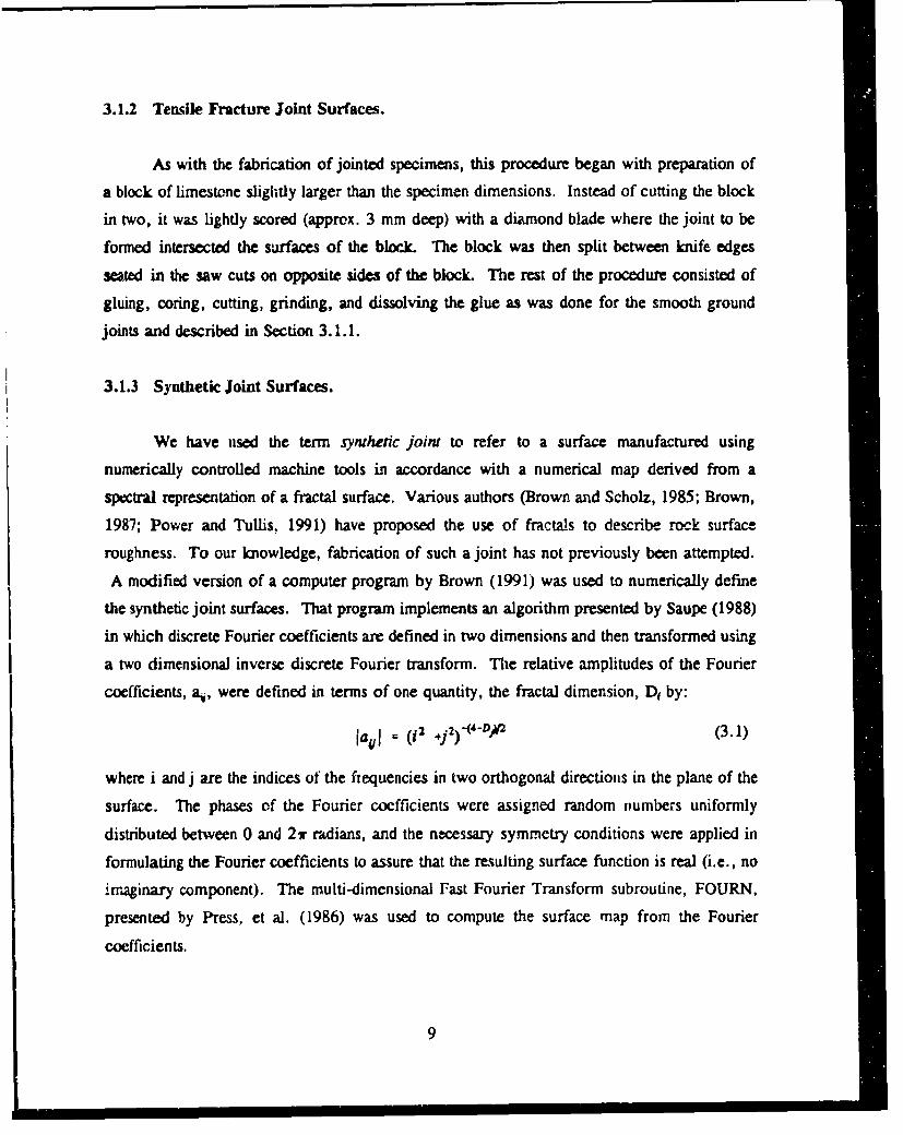
3.1.3 Synthetic Joint Surfaces.

We have used the term synthetic joint to refer to a surface manufactured using

numerically controled machine tools in accordance with a numerical map derived from a

spectral representation of a fractal surface. Various authors (Brown and Scholz, 1985; Brown,

1987; Power and Tullis, 1991) have proposed the use of fractais to describe rock surface

roughness. To our knowledge, fabrication of such a joint has not previously been attempted.

A modified version of a computer program by Brown (1991) was used to numerically define

the synthetic joint surfaces. That program implements an algorithm presented by Saupe (1988)

in which discrete Fourier coefficients are defined in two dimensions and then transformed using

a two dimensional inverse discrete Fourier transform. The relative amplitudes of the Fourier

coefficients,;a, were defined in terms of one quantity, the fractal dimension, D, by.

la 4,1= 2 j-(4-DjM (3.1

where i and j aire the indices of the ftequencies in two orthogonal directions in the plane of the

surface. The phases of the Fourier cocfficients were assigned random numbers uniformly

distributed between 0 and 2 1r radians, and the necessary symmetry conditions were applied in

formulating the Fourier coefficients to assure that the resulting surface function is real (i.e., no

imaginary component). The multi -dimensional Fast Fourier Transform subroutine, FOURN,

presented by Press, et al. (1986) was used to compute the surface map from the Fourier

coefficients.

9

After the shape of the surface was computed, its amplitude was scaled by a multiplicative

scale factor. In the literature, the amplitude of a rough surface is often specified in terms of its

standard deviation, which is simply the standard deviation of the data set consisting of the

surface height at each point on a square grid of fine enough spacing to represent the frequency

content of the surface. This measure of surface roughness can be somewhat deceptive because

its value for a given fractal surface is dependent on the in-plane extent of the area considered.

To understand this, consider the two-dimensional problem of roughness imposed on a straight

line. If the roughness is simply sinusoidal with constant frequency and amplitude, then the

standard deviation of the height of roughness is independent of sample size as long as a large

enough sample is taken to average over several cycles. However, if the surface is fractal, there

is some amplitude at all frequencies (obviously, this has some limits in representing real

surfaces) and the amplitude increases with decreasing freiuency. For a givin fractal dimension

and amplitude, a larger sample will contain lower freqencies and thus larger amplitudes.

The specific surfaces reported here were generated from a 1024 x 1024 matrix of

complex Fourier coefficients derived using Df = 2.5, resulting in a 1024 x 1024 surface

function. It was scaled to have a standard deviation of 1.58 mm and then truncated to 320 x 640

points and assigned a point spacing of 0.20 mm, corresponding to a 64-mm x 128-mm surface.

Once the numerical surface map was computed, a second program was used to generate

instructions for a numerically controlled three-axis milling machine. This involves consideration

in three dimensions, of the shape of the cutter relative to the rough surface. The frequency

content of the surface map generated with 0.20-mm point spacing includes concave regions with

radii too small to be cut with the available tooling. Thus, for each cutter movement, all map

points within the radius of the cutter were checked to compute the new cutter position based on

the criterion that no extra material be removed. As a result, some material that the numerical

map specified for removal was left in the bottoms of the small-radius concave regions because

the tool was too large to reach it. This results in imperfect mating of the portions of the surface

that could be cut by the tool. In hindsight, some other criterion might have given better results.

10

The surfaces used in this work were machined in two passes. On the first, a 1/8-inch

(approx. 3 mm) diameter solid carbide ball end mill was used with the geometry specified at

points spaced 0.80 mm each way while ensuring that no extra material was removed at the

intermediate positions. On the second pass, points were specified at the original 0.20-mm

spacing and a 1/32-inch (approx. 0.8-mm) cutter of the same type was used. The overall

procedure for fabrication of the synthetic joints closely follows the procedure for smooth ground

joints described above, except that th-. surface machining is done in place of grinding.

3.2 SURFACE GEOMETRY MEASUREMENT.

A laser profilometer was assembled for the purpose of measuring the topography of the

various rock surfaces. The rock to be prefiled is first attached to a fixture on an X-Y table

which can be positioned by stepper motors under computer control. The table can be positioned

with a resolution of 0.01 mm anywhere in its range. Attached to a static frame above the table

is a non-contacting position sensor that measures the height of the rock surface relative to a

reference plane. The position sensor is a commercially available unit that works on the principal

of laser triangulation. It projects a laser spot downward on the vertical and receives the

reflected light at a different angle. Depending on the height of the point where the light is

reflected, it is focused on a different portion of the detector. The detector circuit converts the

measurement to an analog voltage which is input to a 16-bit analog to digital conversion card

in the computer. The system has a vertical resolution of 0.001 mm over a range of 20 mm.

The size of the laser spot projected by the non-contacting position sensor is of the order of 0.1

mm. Thus, the spectral amplitudes at frequencies in excess of 10 cycles//mm are probably not

acccurate.

In order to fully characterize the geometry of a joint surface of the type used for

mechanical property and fluid flow testing, it would be necessary to make a large number (of

order 10') of height measurements. This was judged to be cost prohibitive. As an alternative,

the profiling pattern illustrated in Figure 3-2 was defined. It includes profiles in two

perpendicular directions, and consists of ten 2048-point traces, with 0.01-mm spacing between

points, arranged in four lines. Figure 3-3 presents measured profiles of a tensile fracture joint.

11

The profiles are arranged on the plot to suggest the way they were measured, an 82-mm pass

along the axis of the specimen and 20.5-mm passes on either side of center, and a 41-mm pass

across the narrow dimension of the surface and 20.5 mm passes on either side. Corresponding

data are presented for a synthetic joint in Figure 3-4. The profiles shown in Figures 3-3 and

3-4 were processed to determine their spectral characteristics. The data in each figure were

separated into six 2048 point (20.5 mm) traces, and th-2ý mean was subtracted from each. A Fast

Fourier Transform (FF1) was then computed from each 2048 point trace. The FF1 computation

was performed with the subroutine, FOURI, from Press, et al. (1986). The values plotted in

the figures labeled FFT amplitude are the magnitudes of the complex array, H,, defined by:

N-i

H , ht 2IN (3.2)k-0

wherc: hk - ka element of surface height array for one line

i f the square root of-I

k - index of the roughness array

n = index of the FFT array

N = number of points in profile array (here, N = 2048)

To avoid confusion, the computed FFT amplitudes have not been normalized, and thus their

units are mm, the same as the imput array. As with the standard deviations of a surface, caution

must be exercised in comparing FF1 amplitudes as their value for a given surface depends on

the size of the input array. The amplitude spectra of three representative transforms are

presented in Figures 3-5 and 3-6 for the tensile fracture and synthetic joints, respectively. In

those figures, successive traces are offset horizontally by a factor of ten for clarity. There is

clearly significant variation between individual traces from the same surface, and many of them

would be impossible to fit unambiguously with a straight line. In order to obtain a more

representative and useful characterization of the surfaces, all ten FFTs for each surface were

averaged at ..'ach frequency point. The resulting average spectra are plotted for comparison

without shifting in Figure 3-7. The slopes, and thus fractal dimensions, of the two different

types of joint surfaces are very similar, but the synthetic joint has higher amplitude by

approximately 60%.

12

Power and Tulis [1991] present the following relationship between the slope of the FFT

amplitude spectrum, f, and the fractal dimension:

D/= 0 + 2 (3.3)

From Figure 3-7, the synthetic surface has a slope of 1.0, corresponding to fractal dimension

of 2.5 as specified in construction of the numerical map for machining the surface.

13

Ground

Tensile

Fracture

Synthetic

Figure 3-1. Photographs of the three types of surfaces u, r r' joint testing.The smallest divisions on the rulers are mm.

14

Axial Scans

Lateral Scans

Figure 3-2. Layout of the profile lines for characterization of joint surfaceson shear test specimens.

15

I I--_~ I I , I =.,SI i I

__

CQ a3

S iI; -"-.

I I a.

I I I I

I• [ 1tU

Si I a. _ U

Q- )

oI I

16.o'(I '.o I I .. . . , .

I m u IqlH(~ m o1 K -

cn

0 "'

3 ( Ia - [_

.4 - -- , I-o

[o I0 i4

K- 4

_ I _____ __. . .. ___ ___17

]77

C)

-4 4)

s-i-

~q2

.. .. , I ...... . I 11 11 1 1111l1 .. . - L I ... . . I ...... . I -_o o ~ h

o .-i- 0 0S-d 0

apnjjduy V IAI

18

.I ,I I0

CZ:%

C

0}

0m

0

apiilTldu-V j, .. j

1.9

e ! I I I I I I I I111 I I I I I 1 91 1 I I111 I I I 1I

• " • U

o "

o

. -•- 00

ID0

20 •_0

SECTION 4

TEST PROCEDURES

This section of the report describes the procedures used to prepare and instrument test

specimens, loading methods for the various types of tests, and data recording and processing

techniques.

4.1 SPECIMEN PREPARATION.

The test specimens were prepared from the blocks of Salem limestone described in

Section 2. A water-cooled diamond coring bit was used to cut cylindrical samples 48 mm in

diameter with their axes perpendicular to the bedding planes of the limestone. For intact

specimens, the cores were cut to length on a diamond saw, and their ends were ground flat and

parallel on a machinist's surface grinder with a 170 grit diamond wheel. The finished specimen

lengths were in the range of 96-100 mm. The jointed specimens, which were the same size as

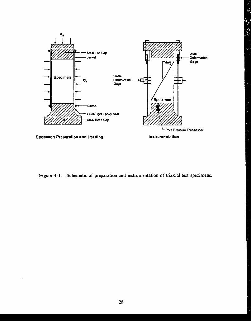
the intact ones, were prepared as described in Section 3. In all tests, th, ecimen was :ealed

inside a membrane, or jacket, to separate it from the confining fluid. At pressures of 10 MPa

and above, a jacket of heat-shrinkable polyolefin tubing was used for this purpose. Tests

performed on the polyoletin jacketing material indicate that it can add a maximum of

approximately 0.2 MPa of additional confinement under large radial expansion. For confining

pressures of 20 MPa and larger, this error of I % or less was considered acceptable. A less stiff

latex membrane was employed in its place at lower pressures. In either case, the jacket was

sealed to the hardened steel endcaps at both ends using epoxy adhesive and wire clamps, as

shown in Figurc 4-I.

For joint testing in this configuration, it is essential to minimize the friction between the

ends of the specimen and the steel endcaps. This is accomplished through the use of lubricating

materials as shown in Figure 4-1. The endcap lubrication system consists of a 0.013-mm layer

of copper against the specimen and two 0.05-mm layers of teflon lubricated with a drop of

kerosene. Evaluations made under simulated test conditions, have shown that the coefficient of

fhiction across the specimen-endcap interface is less than 0.0,.

21

4.2 MOISTUIRE CONTENT PREPARATION.

In the course of this work, tests were conducted on specimens having moisture conditions

ranging from dry to fully saturated. The following subsections describe the procedures for

preparing rock test specimens for those conditions.

4.2.1 Unsaturated Specimens.

In preparation for testing in the dry or unsaturated conditions, specimens were held in

a labor-Atory oven at 105°C for at least 24 hours. Upon completion of this step, the rock was

considered to have zero moisture content. At that point the specimen was weighed and

measured. As discussed in Section 5.1, the oven dry specimens have been shown to exhibit

higher unconf'ied strengths than i tally id'eitical specimens with a few pecent water content.

Since the in situ structures that motivate tL i study are nearly always wet, the strengths of

interest are those of the wet material. Thus, Lhe majority of tests were run with approximately

2% water content by weight. For the limestone with 0.169 porosity, this corresponds to a

degree of saturation of approximately 0.3, i.e. 30% of the void space of the rock was filled with

water. To achieve this condition, the oven dry specimen was sealed in a plastic bag with the

necessary quantity of water for approximately 2 hours.

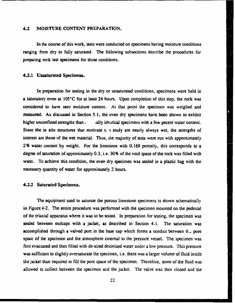
4.2.2 Saturated Specimens.

The equipment used to saturate the porous limestone specimens is shown schematically

in Figure 4-2. The entire procedure was performed with the specimen mounted on the pedestal

of the triaxial apparatus where it was to be tested. In preparation for testing, the specimen was

sealed between endcaps with a jacket, as described in Section 4.1. The saturation was

accomplished through a valved port in the base cap which forms a conduit between d.., pore

space of the specimen and the atmosphere external to the pressure vessel. The specimen was

first evacuated and then filled with de-aired deionized water under a low pressure. This pressure

was sufficient to slightly oversaturate the specimen, i.e. there was a larger volume of fluid inside

the jacket than required to fill the pore space of the specimen. Therefore, some of the fluid was

allowed to collect between the specimen and the jacket. The valve was then closed and the

22

pressure vessel filled with oil and pressurized to approximately 4 MPa. Because of the excess

fluid under the jacket, the pore pressure in the specimen at that point in the procedure was the

same as the confining pressure. During this pressure soak phase, any minute amounts of air

remaining in the pore space of the rock went into solution in the water. Prior to beginning the

test, a small amount of water was released from the specimen, resulting in a drop in pore

pressure to approximately 1.6 MPa. The ratio of pore pressure to confining pressure of 0.4 was

selected as the starting condition because it approximates the stress ratio that would exist if a

fully saturated but unstressed specimen was loaded hydrostatically without drainage. This is

discussed further in Section 8. Since the valve that controls the pore fluid flow is located in the

base cap, approxinmately 5 mm from the base of the specimen, the dead volume of fluid is

approximately 1% of the pore volume of the specimen, and the compliance of the saturation

system is negligible.

4.3 LOADING.

The triaxial test apparatus used to conduct these tests can apply two independently

controllable components of load. The specimen is surrounded by a pressure vessel. When

confining fluid is pumped into the vessel, the resulting pressure acts uniformly over the entire

surface of the test specimen. There is also an axial loading piston that penetrates the vessel

through a seal and bears on the top cap of the prepared specimen. The loading piston imposes

an axial deformation on the specimen, resulting in an incremental axial stress.

In this program, two different loading schemes were employed, as described in the

following subsections.

4.3.1 Triaxial Compression.

The majority of testing was done under conventional triaxial compression test conditions,

i.e. the confining pressure was held constant while a compressive axial deformation was

imposed. Where possible, loading continued until an axial deformation of at least 5% of the

specimen length was reached. Axial strain rates ranging from lOr to 10-2 s' were used.

23

4.32 Hydrostatic Compression.

In the hydrostatic compression tests, the jacketed specimens were simply loaded by fluid

pressure with no additional loading from the piston.

4.3.3 Unlaxial Strain.

In a uniaxial strain test, the specimen is compressed axially while controlling the

confining pressure such that no specimen deformation is allowed in the radial direction. The

loading was controlled based on real-time feedback from the deformation instruments to achieve

a specified deformation history.

4.4 INSTRUMENTATION.

Electronic instruments were used to measure the confining stress and axial load applied

to the specimen, and the resulting pore pressure and sr imen deformation.

Confining pressure measurements were made with a commercial pressure transducer with

the sensing element consisting of a strain gaged diaphragm. A load cell inside the pressure

vessel, located between the top cap of the specimen and the loading piston was used to measure

the axial load. Since it was inside the pressure vessel, it was not subject to errors due to seal

friction. It was, however, subjected to the confining ,sure. Its design, consisting of a full

strain gage bridge, makes the internal load cell, in the ideal case, insensitive to the confining

pressure. Since it is not ideal, there is a slight sensitivity which has been quantified and a

correction was applied during data reduction.

The pore pressure was measured by a piezoresistive pressure transducer located in the

basecap as illustrated in Figure 4-1. The pore pressure transducer was located immediately

adjacent to the base of the specimen, minimizing the dead volume of fluid, and hence

minimizing extraneous compliance.

24

Specimen deformations were measured with Linear Variable Differential Transformers

(LVDTs). Each specimen was instrumented with three LVDTs as shown in Figure 4-1. Two

LVDTs were attached to the base caps on diametrically opposite sides of the specimen to

measure axial deformation. Since the axial LVDTs were mounted to the endcaps, the resulting

displacement measurement included the deformation of the endcaps and lubricating materials in

addition to the intended axial deformation of the rock specimen. A correction was applied

during data reduction to eliminate the effect of endcap and lubricating membrane deformation

from the measurements.

The third LVDT, used to monitor radial deformation of the test specimen, was mounted

in a reference ring at the specimen's mid-height. In the conventional triaxial compression tests,

all of loading and measurements take place at a constant confining pressure. Thus, there should

be negligible change in the thickness of the jacket as the test progresses, and the radial

deformation measurements are made on the outside of the jacket. In contrast, the strain path

tests require that the confining pressure change throughout the test, resulting in variations in

jacket compression during the test. In those tests the radial deformation measurements were

made using studs glued to the specimen through holes in the jacket and sealed to the jacket with

o-rings. In this manner, error due to jacket compression was eliminated.

4.5 DATA RECORDING AND REDUCTION.

All channels of instrumentation were digitally recorded using a 12-bit analog-to-digital

converter. Since the strain rates in the various tests varied over orders of magnitude, sampling

rates were adjusted to provide the necessary resolution in each test. The digitized data were then

multiplied by the appropriate calibration factors to convert to engineering units and, where

necessary, corrected for pressure effects.

The axial stress was computed by dividing the measured axial load by the original cross

sectional area of the test specimen. The triaxial compression tests performed at pressures of 50

MPa and greater are presented in terms of true axial stress (or stress difference) which is

computed by dividing the axial force (or load difference) by the current cross sectional a.°m at

25

each time point. The reported axial deformation was computed as the average of the results of

the two axial LVDT measurements. It was corrected for endcap deformation and thus represents

the change in length of the entire specimen. When sliding occurs alone a joint, the reference

ring holding the radial LVDT rotates away from the horizontal, resulting in error in the radial

deformation measurement. A correction based on the amount of axial deformation was applied

to the radial measurement to correct for the rotation error.

For undrained tests, the effective stress was computed by subtracting the measured pore

pressure fhm the total stes.

Additional processing was required to compute the joint response quantities. The shear

and normal stresses on the joints were computed as follows:

o ad= + o rF 2 0 (4.1)

01- co 22 2

a sin 2e (4.2)

2

where: a. = normal stress on joint (+ is compressive)

a, = axial stress on the specimen

o, = radial stress on the specimen = confining pressure

0 = joint angle with respect to the core axis

S= shear stress on the joint

The normal and tangential deformation of a joint were computed by first finding the

difference between the overall deformations of a specimen containing a joint and the

corresponding deformations of an intact specimen from an adjacent location in the same horizon.

This computation was made only for those jointed specinmens that failed by joint sliding. Since

the stress supported by the jointed specimen was limited by the joint failure mode, the intact

portions above and below the joint did not fail. Therefore, only the pre-failure portion of the

intact test data was used to make the correction for deformation of the intact material. In

26

making this calculation, the intact deformation record was interpolated to the same stress levta.;

as in the jointed test data. Once the response of the joint was isolated in terms of axial and

radial deformation, the following transformation was made to arrive at deformations normal and

tangential to the joint:

AM = A sin e + A,P o e (4.3)

As = Ad cm e - A, sin e (4.4)

where: A, = joint normal deformation; positive implies joint compaction

A. = axial deformation due to joint; positive implies the ends of the

specimen move toward each other

4 = radial deformation due to joint; positive implies opposite sides of the

specimen move toward ech other

, = joint tangential deformation; positive implies sliding of the joint such

that the ends of the specimen move toward each other

27

a

t---St". Top Cap Axial

Specimen aFOo-.tlonGage

"SpecimenClamp

// / . ~Flu-Tight Epoxy SeWi/

/ // - stoo Ca2p

Pore Pressure Trnsducer

Specimen Preparation and Loading Instrumentation

Figure 4-1. Schematic of preparation and instrumentation of triaxial test specimens.

28

Wntar 1Reservoir

Pressure Vessel

Jacketed Test Specimen

, Valve in Base Cap

Water Valve7 '"

Vacuum Valve

Figure 4-2. Schematic of system for saturation of porous triaxial test specimens.

29

SECTION 5

MECHANICAL PROPERTIES OF INTACT LIMESTONE

The mechanical properties of Salem limestone have been studied extensively under

various DNA-sponsored contracts (Chitty and Blouin, 1990, 1992, 1993; Cummings, 1991).

In spite of the fact that it is locally a very uniform material, values of porosity ranging from

0.12 to 0.17 have been observed. Since a complete set of mechanical property data was not

available for Salem limestone with the same porosity as the specimen material (n = 0. 17), a

limited series of standard and special tests was run to piavide a characterization of the intact

material. This includes unconfined compression tests at various water contents, unconfined

compression tests in which the test machine was specially modified and controlled to measure

the post-failure behavior of the material, triaxiai compression tests at a range of confining

pressures up to 400 MPa, hydrostatic compression tests, and uniaxial strain tests. This

subsection presents the results of those tests.

5.1 UNCONFINED COMPRESSION TESTS.

Two sets of unconfined compression tests were performed for different purposes. Near

the beginning of the project, a series of tests was performed to investigate the influence of water

content on the mechanical response of the limestone. Those tests are documented in Section

5.1.1. A second set of unconfined compression tests, described in Section 5.1.2, was performed

to determine the post-fai!urc response of the material.

5.1.1 Unconfmned Compressiou Tests at Various Water Contents.

In previous work, (Chitty and Blouin, 1993), it was found that the unconfined strengths

measured for limestones exhibited a strong dependence on water content, with oven dry

specimens having significantly higher strength than those with higher water contents. In order

to quantify that effect for Salem limestone, a series of 14 unconfined compression tests was

performed on specimens from the same block of limestone. These tests were done at water

contents (mass of water divided by mass of dry rock) ranging from 0 to 0.055, corresponding

30

to degrees of saturation (volume of water divided by volume of void space) of 0 to 0.72. Thl

results of those tests are summarized in Table 5-1 and plotted in Figure 5-1. The values for

elastic modujus and Poisson's rAtio presented in Table 5-5 were computed by least squares fits

to the test data over a range of 25-65 % of the unconfined strength. Consistent with the previous

results, the three oven dry specimens had strengths averaging 58.2 MPa while the eight with

water contents in excess of 0.01 had strengths averaging only 48.3 MPa. The elastic moduli

were also higher for the dry specimens.

It is sometimes reported in the literature that rocks are tested in the 'air dry* or 'lab dry"

condition. In order to quantify those expressions, an experime'nt -', performed on a group of

27 specimens that had been exposed to ambient condl,,icnib in the ARA laboratory for at least two

weeks since coring (using water as coolant) and grinding. They were weighed, oven dried at

105 C for 48 hours, and then reweighed. The moisture contents thus determined averaged

0.00042 with standard deviation of 0.00006. Based on the data presented in Tablc 5-1, the air

dry specimens clearly have moisture contents in a range that would be expected to exhibit

unconfined strengths sig.ificantly higher than moist specimens.

As a result of this study, we performed all tests on unsaturated specimens at a water

content in excess of 0.01 in order to eliminate any influence of an over-dry condition on test

results.

5.1.2 Post-Failure Response of Limestone in Unconfined Compression.

In a typical unconfined compression test, the objectives are to measure the strength of

the material and possibly the elastic modulus and Poisson's ratio on initial loading. With these

as objectives, it is only necessary to iml • increasing axial strain (shortening) on the

specimen until the load supported by the specimen peaks and begins to decrease. In such a test,

strain energy increases in the test machine as the load in the specimen increases. Under typical

circumstances, that energy is released into the specimen as it fails, causing a sudden dynamic

axial deformation, and making it impossible to measure the post-failure response of the

specimen. The tests reported here weie conducted using procedures specially developed to

31

prevent the release of energy into the specimen upon failure and make it possible to record post-

failure response.

Two modifications to the usual test techniques were implemented to accomplish this.

First, an aluminum alloy stiffener ring was installed concentric with the test specimen and loaded

in pardlel with it. This is illustrated in Figure 5-2. Thus, when the specimen failed, the load

in the test machine was transferred to the stiffener ring. Since the ring was stiffer than the test

specimen, even before failure, it significantly limited the elastic rebound of the test machine

upon specimen failure. A small load cell was placed atop the specimen within the ring so that

it measured only that portion of the load applied to the specimen. In order to stay within the

elastic range of the stiffener ring, the components of the system were sized such that

approximately half of the rock specimen's elastic deformation was imposed before the stiffener

began to be loaded.

The second modification was a special configuration of the test machine's servo-control

system. In the usual control mode, a displacement transducer attached to the loading piston is

used as feedback for the control system. While this is adequate under momt circumstances, the

control requirement for this type of test was very rigorous and the deformation of the load frame

made it impossible to achieve the necessary precision in control. Thus, it was necessary take

the feedback signal from the displacement transducers mounted directly to the steel endcaps on

either end of the test specimen. Because the transducers were mounted to the endcaps and not

directly to the specimen, they also measured some amount of endcap deformation. It is usual

practice to correct for this in post-test processing. However, for these tests, it was necessary

to include a correction for endcap deformation in the computation of the control signal. An

attempt was made to avoid this complication by attaching the axial deformation transducers

directly to the specimen. While this worked well during the elastic portion of the test, the

attachment points tended to slip upon failure of the specimen, ma g subsequent control

impossible. The criterion used to control the test was to move the ends of the specimen closer

together at a constant rate.

32

Figure 5-3 presents an overlay of stress-strain curves from six nominally identical tests.

Of the six, four fall very close together while one is significantly stronger and one is

significantly weaker. In all of theses unconfined tests, the softer portion of the stress-strain

curve on initial loading is attributable to seating of the enccaps against the ends of the specimen.

Appendix B presents individual plots of these tests, including radial strains measured at two

locations 900 apart.

5.2 TRIAXIAL COMPRMSSION TESTS.

A series of triaxial compression tests at pressures ranging up to 400 MPa was performed

to define the strength envelope of the Salem limestone in the intact condition. Those tests are

documented in Section 5.2.1. Some of those test results were used along with tests on jointed

specimens to derive the joint deformation data presented in Section 6. A brief zest series,

described in Section 5.2.2, was also conducted to investigate the effects of specimen a~pcct ratio

and ePd conditions on the measured strength and deformations. Additional triaxial compressio,

tests on intact specimens wLrc performed to investigate the influence of strain rate, and those

are. described in Secdon 7.

5.2.1 Intact Strength Determination.

The strength of the intact Salem limestone was determined through a series of triaxial

compression tests at pressures ranging from zero (unconfined) to 400 MPa, as summarized in

Table 5-2. The triaxial compression testing emphasized the pressure regime of interest to joints,

i.e. confining pressures of less than 50 MPa. Figure 5-4 presents axial stress-strain curves from

triaxial compression tests at confining pressures ranging from 0 to 35 MPa. For those tests in

which the stress difference reached a maximum and then decreased, the state of stress at that

naximum was taken as a point on the strength envelope. Above the brittle-ductile transition

(-35 MPa confining pressure), where the stress did not pezk during the tests, the stress state

(in terms of true stress) corresponding to 15% axial strain was assumed to define the strength

envelope. In the low pressure (brittle) regime, where failure occurs at strains less than 1 %, the

difference between true and engineering stress is insignificant. Strength data for the full range

33

of pressures arc presented in Figure 5-5, and Figure 5-6 shows more detail in the low pressure

range. Data from the triaxial compression tests that were not used for computation of joint

deformations are presented in Appendix C. The data from joint-related t-iaxial compression tests

on intact specimens are included with the joint tests in Section 6 and related appendices.

5.2.2 Investigation of Specimen Aspect Ratio and End Conditions.

In previous work (Chitty and Blouin, 1992), the techniques described in Section 4 were

developed to reduce the friction between the ends of the rock specimen and the steel enacaps

through which the axial load is applied. For a triaxial compression test in the ductile regime,

this lubrication technique produces uniform radial expansion over the height of the specimen

rather tha the barrel shape that typically results when the specimen-endcap interface is not

lubricated. This approach has also worked well to reduce friction for shear testing of jointed

specimens. For tests on intact specimens in the brittle regime and around the brittle-ductile

transition, tle reduced effective confinement at the ends of the specimen resulting from the

reductior in end friction apparently makes it possible for failure to be initiated at locations other

than at specimen mid-height. If radial deformation gages are only installed at or near the center

of the specimen and failure is initiated near one of the ends, then the radial expansion in the

failure zone will not be measured. This effect has been observed in many triaxial compression

tests on intact specimens at confining pressures of in:',rest to joint strength investigation.

Measurements of the permanent volume change of a material following loss of strength are

important for constitutive modeling of rocks and soils to support explosive effects calculations,

and accurate axial and radial deformation measurements are essential for definition of the volume

change of the specimen under load. Further, Chitty and Blouin (1990) demoinstrated that the

non-urifofn radial deformation of a triaxial compression specimen is accompanied by a non-

uniform axial strain field, making accurate computation of the volumetric behavior of the

specimen impossible.

In order to investigate techniques for measurement of post failure volume change

behavior, a brief series of triaxial compression tests was performea hi the bii•LIe-ductile

transition pressure range (25 MPa confining pressure). Included were a "standard" test with

34

unlubricated endcaps and a 2:1 length to diameter (LID) ratio, a test with 2:1 L/D and lubricated

endcaps, and one with 1:1 LID and lubricated endcaps. Figure 5-7 presents the initial portions

of the curves of stress difference plotted against axial and radial strains. From that figure it is

apparent that there were no significant differences in either strength or deformation among the

three test results. It is only in the post-failure portion of the tests that the differences become

apparent. At this confining pressure (25 MPa) there is very little change in stress difference

with increasing axial deformation after the peak strength has been reached. Thus, plots of

strains against sutess difference are not a good basis for comparisons among the tests in the post-

failure region. As an alternative, consider the radial swair plotted as a function of axiad strain.

Figures 5.8 through 5-10 present such plots for the three tests described in this paragraph. In

all cases, the plotted axial strain is the average over the entire specimen length, i.e. the change

in length of the specimen divided by its original length. From the test :measurements, there is

no way of knowing whether the axial strain is uniform over the specimen length. Further,

Figures 5.8 and 5.9 include multiple radial deformation measurements, representing different

heights on the specimens. In all three tests, the radial gages give consistent readings for the

initial approximately linear portions of the tests represented by the first half percent of axial

strain

In the case of the specimen with unlubricated endcaps, shown in Figure 5.8, the three

radial gage readings diverge, and never rejoin, indicating nonuniform radial deformation

developing throughout the post-failure portion of the test. By the time the average axial strain

reached II%, two of the radial gages had gone off scale at over 10% radial strain while the

third was indicating only about 4% radial strain. The test widh lubricated endcaps presents a

very different picture. Following failure of the specimen, ti~c upper half of the specimen

underwent a significant radial strain while the radial strain in the lower half remained essentially

constant at the level of the initial failure until the axial strain reached approximately 5 %. At this

point, the lower half of the specimen began expanding radially while the radial strain in the

upper part remained relatively constant. By about 12% axial strain, the two radial readings were

essentially identical, indicating a nearly uniform strain field over the entire specimen. The

specimen with unlubricated ends never reached that condition, and exhibited very nonuniform

radial deformations at the conclusion of the test.

35

The results of the test with lubricated ends can be interpreted in the following way.

Initially, there awe uniform axial and radial strain fields throughout the specimen. At the peak

of the stress-strain curve, where the strength of the material is reached, there is a localized

failure somewhere in the specimen. In tests with lubricated ends, this has been observed to

occur toward one end of the specimen. Possibly, this is a result of the relatively soft lubricating

materials deforming more than the rock and applyng a slight outward radial traction to the ends

of the specimen. In general, we hive observed that failures, wherever they occur in the

specimen, to be localized over a length of specimen equal to roughly one specimen diameter.

Once this localized failure is initiated, the stress in the specimen drops below the failure level,

and the rest of the specimen remains intact. Eventually, the radial expansion in ith lucalized

region increases the cross sectional area to the point that it will support slightly more load than

was required to initiate failure, resulting in sequential failure of the previously intact material

in the opposite half of the specimen. With enough axial deformation, the conditions of the

material in the two halves of the specimen become nearly the same. For the portion of the test

between initiation of failure and the time the radial strain records from either half rejoin, the

material in the un-failed half is elastic while the failed half undergoes significant plastic

deformations. Thus, it seems reasonable to assume that the large increase in indicated axial

strain is largely a result of deformation in the failed half of the specimen, and neither of the two

curves shown in Figure 5.9 correctly represents the strain condition in either half of the

specimen. This is a serious drawback for constitutive modeling where the post failure

volumetric behavior of the material is very important.

For defining the post-failure deformation, it would be very. desirable to conduct a test in

which the specimen deforms uniformly over its entire volume. Since. the failed zone appears to

naturally occur over about one diameter of specimen length, it was hypothesized that this could

be accomplished by testing a specimen with L/D equal to approximately one. Traditionally, an

L/D of two has beeAi used in an effort to avoid end effects. However, if lubrication of the ends

can alleviate that problem, t1 en the test may provide more representative post-failure

deformation information. The relationship between radial and axial strains presented in Figure

5-10 is the result of such a test. The curve lies between the two shown in Figure 5.9 for the

test with I./D = 2, and has a slope over the entire post-failure range that is approximately equal

36

to the equivalent slope in the part of the test on the long specimen where both radial gages were

reading the same. The short specimen exhibits more radial strain than the long one at equal

axial strains, the reason for which is unknown. However, we judge results from the short (LID

1) specimen to be more representative of the actual material behavior than either of the other

two tests. Figure 5-11 compares volumetric strains computed using the radial and axial

deformation measurements from the three tests and plotted against average axial strain. Where

multiple radial deformation measurements were made, the figure indicates which was used in

the volume strain computation. There are very significant differences among the volumne strains

derived from the throe tests. We believe that information derived from the test on the short

(LID = 1) specimen with lubricated ends best represents the material's actual respox"<. This

approach is only applicable at confining pressures near the brittle-ductile trL isition where the

failure is localized but the specimen does not fracture into multiple pieces.

While the study described here is far from an exhaustive investigation of the subject, we

believe that most accepted test approaches result in nen uniform specimen deformations, which

in turn result in errors in volumetric strain determination. In view of the importance of the post-

failure volumetric behavior in constitutive modeling, this subject deserves further investigation.

A test on a specimen with LID = I and a lubricated end does appear to be a useful technique

for obtaining more nearly uniform strain fields. A similar suite of tests were performed at 50

MPa confining pressure. Those tests exhibit the same trends and are included in Appendix C.

5.3 HYDROSTATIC COMPRESSION TESTS.

Six Salem limestone specimens were tested in hydrostatic compression to a maximum

pressure of 400 MPa. One test was performed on a specimen in the oven dry condition and rest

had 2.5% water content. The hydrostatic compression tests are summarized in Table 5-3.

Figure 5-12 presents a typical pressure - volume strain curve. The relationship between radial

and axial strain for the same test is shown in Figure 5-13, which clearly illustrates the lack of

isotropy under hydrostatic loading. Once the hydrostatically loaded specimens begin to exhibit

plastic deformation, the specimens compact significantly faster in the radial direction. Also

shown in Figure 5-13 is a point indicating the permanent strain at the conclusion of the test as

37

determined from post-test measurements of the specimen. The post-test measurement validates

at least the final instrument readings, and confirms the anisotropy. The complete set of test data

is presented in Appendix C.

5.5 UNIAXIAL STRAIN TESTS.

Specimens of Salem limestone were loaded in uniaxial strain up to the point where the

confining pressure reached the ARA system's capacity of 400 MPa, as summarized in Table 5-4.

All were tested with approximately 2.5% water content. A typical axial stress-strain curve is

presented in Figure 5-14, the corresponding relationship between axial and radial stress is shown

in Figure 5-15, and the mean stress-volume (axial) strain relationship is illustrated by Figure 5-

16. Appendix D presents a complete set of uniaxial strain test data.

38

- -- -A-% Vn; n C4 4 n

c r4~ 4' C- 4

Jv -- - - -

. . . . . .0- r'~ 4 C1e4 C4 C1

m 002

_00 00 %00 00 -1--------

2000

C C

(N '4 4 C' . . C

00-0 00 000C4rý 1

00 0 0 <

39

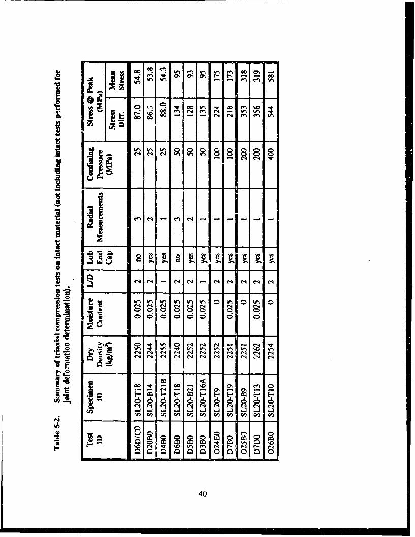
aý en I rn 00 C7CK~ O NO O as ( w~0

4n~~ enenV

C4 M-C

C4N C- 4 4C

M cn

i - o o 0

z~ 0 0'v

eo6 666 40

Table 5-3. Summary of hydrostatic compression tests on intact Salem limestone.

Test ID Specimen Dry Density WaterEID (kglm 3) Content

Y20A1 SL21-T22 2258 0.025

Y17A1 SL21-B19 2251 0.025

YI6A1 SL21-B12 2247 0.025

Y15BI SL21-T1O 2251 0.025

YI5AI SL21-T17 2258 0.025

NIAO SL20-B 11 2253 0m - -

Table 5-4. Summary of unlaxial strain tests on intact Salem limestone.

Test ID Specimen Dry Density MoistureID (kg/mr) Content

U19A1 SL21-T2.0 2249 0.025

U18A1 SL2I-B14 2247 0.025

Y23A1 SL21-T19 2255 0.025

- 4-

0

t co

O0 1 .

-C-,

lo

0 c

00

vUd )

00O0 ) --'

0 .0

0 0

42)

OC 0 I 0 _ I ,

(•dN{) t~u•x•S aA!ss~Jduzo3 p~U~Tuo3Ufl

42

Axial Loading

Load Cell

Specimen ; -

LVDT

StiffeningRing IMI

Figure 5-2. Schematic of the stiffener ring used in tests to determine post-failure responseof Salem limestone in unconfined compression.

43

m -o

U-1

i £

I O

' ' I , ' ' 1 - I ' ' , I ' Il I U

-%- - C

-----

L -// ; - _

C\l0

0 a' Ln C

U'D~~~U v q C) c Q c

(- dW) s sGx1 -- ICtxv

44

1_=

emo

-7 i C~

°I

C)C

0

uCu

U

U) E

"o 0

~1 -

: c u --: 4"5

L. I .-

: - U-

o .. ci ci 0

S/-S.,..J

45.

CA

°A

104

Li

g U"

0E

(,A

460L."C

• .-

(•;) uaaU.) s 0 aa •..

N•

46

L_

cqCOC

E

U tj

U)U

0 CCu

C) Eo o (

0 .0

V-1

I ~Li

0 -1 €"4

1o~ C

0

0 00 G 0

0~ 0

t.2

47u

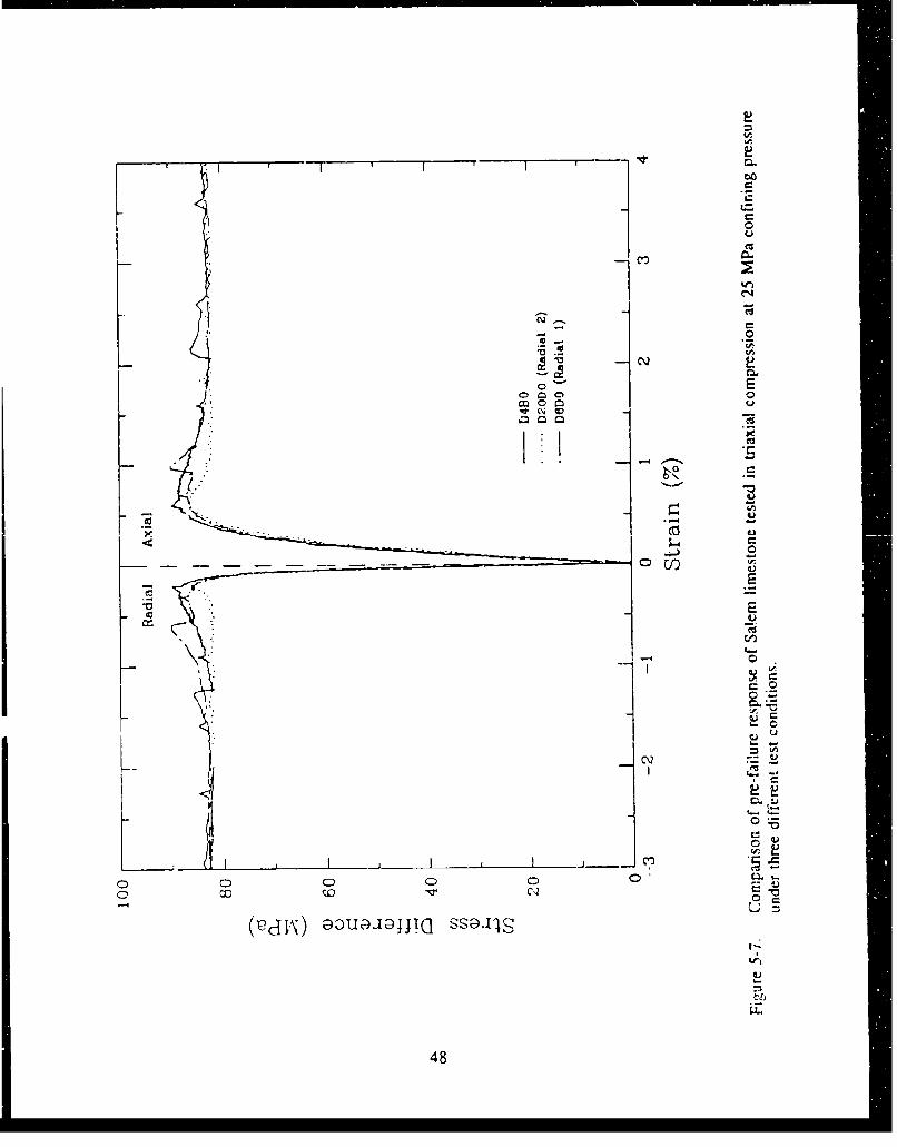
10Cu-cc-2

0

o E

CU)

CD 01 0 .

• I.-.-

cc N

C-- J'

oP

48

SI• • II I a I I • iI •.I ,1 C .u,

C-

E

- 0•

$"o

/5/ ~-•

0) 4)

CDu

:1z]u

0 t0

.- - c . U

(CV uve) >~P~co m , Io

49

4r.=

-

Ia..

c E

00

Tj

-�0

C4

Cu

IU l.

Cu

I && O"•- C

-c ) oJ

.-

!2twIII -• .•

U

50

CUf-.., I c\

Cv 0

0(.o

-4• E0

','

I5,- .

51-

I "-

°C

a- *

I CU ,

'-C

/1

r-0

°•

C4C

I-

11 Cf 1 m c

E

IUI

0

__ 0

522

\ C=.- U-'I. ---.

I C O

.- -.

I-,

I 0

(%) uI•-JcS 3!T•UunlOA

52

C~Cu

4-j

C\2

CD 0 D00

E

o E4.)

-4-

C.)'

V') Ir \

Se= C

53

i q I I I I I ! ! . !0

0

E

-o

*0

cou

V).

-J.•

v o C0 €-

L._

54Cu

54C

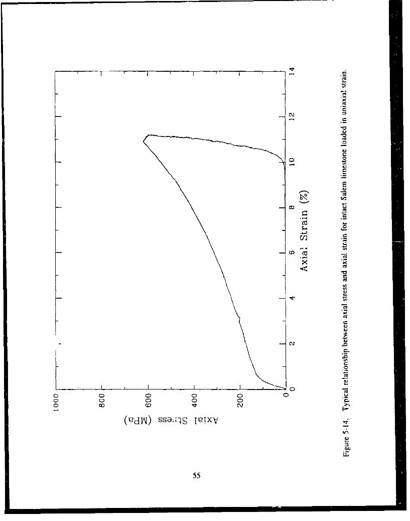
IN•

Cc

0 o

COa -C

U

°Q

o 0

E

U)

.o

55-.

o o 0 C

o cocD ,' • :'-

S [.--,

(•dla) sso:-• T!X( .U,

55)

i J "I-

'-

0 e-

c.)

E

-o ul

C')m ~UPI

4-4

oc

o .UIo O O

00

cio o 0o 0 0

56

0

00

>U

E

C\2

LiL

_ C)

O v

(PdWtl) Ss@-IIS uea~ll

57

i 1 I , ,. , , , i

SECTION 6

MECHANICAL PROPERTY TESTS ON JOINTED LIESTONE SPECIMENS

Strength and deformation properties of the three types of joint surfaces described in

Section 3 were measured by conducting triaxial compression tests on cylindrical specimens with

joints oriented approximately 30° to the axes of the cores. Identical tests were performed on

intact specimens, and the differences in deformations were used to derive measures of the shear

and normal deformations of the joints under load. Table 6-1 summarizes the joint tests

performed, including tests on intact specimens to support determination of joint deformations.

6.1 TEST PROCEDURES.

The test specimens, prepared as described in Section 3, were sealed in side a flexible

membrane which was sealed on both ends to hardened steel endcaps. At confining pressures

below 10 MNPa, the confining fluid was nitrogen gas and a latex membrane was used. At higher

pressures, a heat-shrinkable polyolefin membrane was used in a hydraulic fluid-kerosene mix.

In all cases, lubricating membranes were placed between the ends of the specimen and the steel

endcaps. These consist of a 0.13-mm layer of copper next to the rock and two 0.05-mm layers

of VTFE. This system results in a coefficient of friction of 0.02 - 0.05 in the stress range of

interest. Figure 4-1 is a schematic view of a prepared test specimen, including the lubricating

materials.

The tc.sts reported here were all conducted along a conventional triaxial compression load

path. The confining pressure was raised to a specified level and then held constant while

controlled axial deformation of the specimen was imposed with the piston.

Two diametrically opposite LVDTs (displacement transducers) attached to the endcaps

were used to measure axial deformation of each test specimens. Corrections were applied to the

data for deformation of the endcaps and lubricating materials. Radial deformation measurements

were made with a third LVDT attached to a floating reference ring. In jointed specimens, it was

installed horizontally at mid-height of the specimen in the vertical plane perpendicular to the

)8

plne of the joint. Since all of the measurements were made at constant confining pressure, any

change in men orane thickness in the course of the tests was considered negligible. In joint

tests, a correction was made for tilt of the radial ring due to relative displacement of the

specimen halves.

At low confining pressures, Salem limestone exhibits higher strengths when tested dry

than when moist, but not saturated. Since the objective of this effort is to support modeling of

saturated in situ materials, all tests were conducted on specimens with approximately 2.5%

moisture expressed as fraction of the dry mass of the rock. This amount of water fills less than

half of the available pore space, and thus there is little chance of saturation during specimen

deformation except at higher (100's of MPa) confining pressures.

6.2 STRENGTH TEST RESULTS.

The average unconfined strength of the Salem limestone used in these tests is 58.3 MPa

wk-4-b icsted dry and 48.5 MPa when tested at 2.5% moisture content. To provide a basis for

comparison with the joint tests, the strength envelope of the intact material was determined by

a series of triaxial compression tests on intact specimens. Figure 5-3 presents the stress

difference-axial strain curves for 6 tests at pressures ranging from 1 to 35 MPa, which covers

the range of interest to joint behavior. The behavior of all of the test specimens can be

classified as brittle except for the 35-MNa test which is in the brittle-ductile transition. The

specimens were also instrumented for radial deformation, but the location of the failure is

unpredictable on specimens tested with lubricated endcaps. Thus, the single radial deformation

measurement at mid-height often misses the post-failure radial expansion. For purposes of

computing joint deform tions, this is not a drawback because only the elastic portions of the

deformation records from the intact specimens are used.

Since all of the stress-strain curves in Figure 5-3 exhibit well defined peaks, their

strengths can be defined unambiguously as the states of stress at the peaks of the stress-strain

curve. Figure 5-5 presents the strength points from 9 tests in terms uf stress difference ani

mean stress. For the stress conditions of a triaxial compression test, these are the same, except

59

for a constant multiplier, as the first invariant of stress and the square root of tie second

invariant of the stress deviator, and are defined as follows:

stress difference = of - o, (6.1)

mean aress = (Gs + 2a,)3 (6.2)

where: a. = total axial stress

, =- confining pressure

Suites of stress difference-deformation curves for smooth ground, tensile fracture, and

synthetic jointed specimens are presented in Figure 6-1 through 6-3, respectively. The

deformation quantities plotted there are the overall axial and radial deformations of the jointed

cylindrical test specimen and thus include detormations of both the joints and the intact ma.zrial.

Figure 6-4 through 6.9 present a comparisons of force-deformation curves for tests a.: ', 2, 5,

10, 20, and 35 MPa confining pressures, resTectively, 0:i a!) three of the joih t types oescrilA

above and intact rock. In spite of having A s!hgh igy l.her magnitude of roughness tne synthcotc

joint exhibits a lower strength than the tmnsile fractire. There is also significai-tly moie

deformation associated with the syrdhetic jcint prior to .,'cahing the strength limit. 'These

characteristics are probably due to the imperfect match in the smallest details betwe-n the halve;

of the synthetic joint.

As with the intact tests, the strezs-deformation curves for tensile fracture and synthetic

joints have well defined peak ',4 •WAints indicating the limiting state of stress for the confining

pressure level of that test. in contrast, the smooth ground joints gradually approach a peak

stress level, which then remains approximately constant under further shearing deformation. For

smooth ground joints, that constant stress level was considered to be the strength. In order to

understand joint behavior, the measured stress quantities, axia: stress and confining pressure,

were roiated to obtain the values of shear and normal stress acting on the joint planes. The

equations for the stress rotation are found in any text on mechanics of materials. Table 6-1 lists

60

the st;-ength of each test specimen in terms of the measured stress difference. In addition, the

peak strengths of the joints are listed in terms of the shear and normal stress acting on the joint

at the time of failure. Figure 6-10 presents strength data from joint tests on all three surface

types in terms of the shear and nomal stresses on the joint planes. for the joint tests, it is

possible to plot the strengths as single points because the plane of interest is known. Ii, contrast,

for the tsts on intact specimens, the stress states plot as circles, known as Mohr's circles, with

differe ,ints on each circle corresponding to different orientations of the reference plane in

the corres,,)onding specimen. Sinc- the plane of failure is not precisely known, the strength

env, lope line for intact material in Figure 6-10 was constructed by plotting Mohr's circles for

all of the intact tests and making a judgement fit of a curve that approximates a tangent to all

tests.

The data points indicated by the square symbols in Figure 6-10 are from specimens with

tensile fractured joint surfaces. In all of those tests, failur-. occurred by sliding along the joint.

"The dot-dashed line, which is an approximate fit to those data points represents a stren-th

envelope for the fractured surface. It runs roughly ..arallel to the intact strength and about 5

MPa lower. The h~ghest point shown, at about 46 MPa normal stress, is from a test at 25 MPa

confining pressure. In a similar test, performed at 35 MPa, failure did not occur by relative

displacement along the joint. Instead, there was localized shear banding and radial deformation

characteiistic of tj c faiiure of an intact specimeo a! that confiaiing pressure. This is an

indicAtion that as thc test prog,-ssed, some point on the Mohr's circle reached the intact strength

envelope before the stress on the joint reachod the joint strength envelopc. Vlis is illustrated

in Figure 6-10. 1'le circular segment at the iight side of the figure is the Mohr's circle

rmpresenting the stress slate in the specimen at failure. The line at 30" to the vertical originating

at 35 MPa on the normal stress axis is the stress path expejicwcW by tlic joint as the test

progressed from h)drostatic to failure. TIhe intersection of the joint stress pi,'h with the circle

represents the state of stress on the joint when the stccinten failed elsewhere. Thus, the strength

envelope of the joint must b.- at least slightly higire, than that poirnt.

The strengths derived fromn tests on synthctic (machined) joints are shown a trianlgie:,

on Figure 6 10. Thc fit to thew polil,, falls 3-4 Mi'a bchlw the ternsile fracture strength line aid

i(

has somewhat less curvature. As in the case of the tensile fracture joint, a synthetic joint tested

in tnaxial compression at 35 MPa confining pressure exhibited the same response (strength,

deformation, and failure mode) as an intact .mecimen subjected to the same loading.

The joint strength points from smooth ground surfaces are plotted as circles in Figure 6-

10. In contrast to the curved envelopes formed by the intact, fracture, and synthetic joint data,

the strengths of the smooth ground joints can be well approximated by a straight line passing

through the origin, i.e. Coulomb friction. As with the other joint surface types tested, a triaxial

compression test performed on a smooth ground joint at 35 MPa confining pressure resulted in

a failure in the intact mode rather than by slip of Ohe joint, suggesting that the strength envelope

for smooth ground joints must also pass above the stress experienced by the joint in the 35 MPa

test.

From the stress-deformation curves presented in Figures 6-2 a - ,, it is apparent that

the shear stress supported by the joints with interlocking asperities (ter sile fracture and syniletic)

peaks on initial loading and then diminishes to a residual value as dite asperities are sheamre off.

In addition to the peak strength data, Table 6-1 presents values of residual strength for each joint

test. For the tensile fracture and synthetic joints as well as intact specimens, the residual

strength is the value reached after the peak, when stress difference becomes relatively constant.

For the smooth ground joints, residual strength is the same as peak strength. Figure 6-11

presents the residual strength data for the three different types of joints and intact material. The

strength points for the intut limestone were c( -%uted for the failure plane defined by the point

on the a strength ,n,,elope fi r the particular 2st. For comparison, the peak strength

envelopes for the v;:• , joints and the inta.,! limestone are shown along with the data points

for re"sdual srength. The residual strengflts for intact limestone and tensile fracture and

synthetic joints fall significantly lower than their respective peak strengths. All of the residual

strength envelopes converge to !he peak intac' strength envelope at approximately 75 MPa

noreal stress.

e'I

6.3 JOINT DEFORMATION.

The normal and tangential defornations of the joints under shear loading were inferred

from two tests .hat were as nearly identical as possible, except for the presence of a joint in one

and not the other In joint tests where failure occurred by sliding along the joint, the two halves

remained essentially elastic. Thus, the net deformation of the intact poition of the jointed test

specimen can be approximated by the initial elastic loading region of the corresponding intact

specimen at the same stress difference level. In both the axial and radial directions, the joint

deformation was computed as the difference between the total deformation of the jointed test

specimen and the deformation of the intact specimen under like stress conditions. A vector

rotation was then performed to arrive at components of deformation normal and tangential to the

joint.

Figures 6-12 through 6-14 present joint deformation data for smooth ground, tensile

fracture, and synthetic joint surfaces, respectively. The normal and shear stresses on the joints

are plotted against joint normal and tangential displacements, respectively, for tests at three

confining pressures, 5, 10, and 20 MPa. The tensile fracture joints exhibit essential!y zero

displacement until the strength limit of the joint is reached, at which time slip on the joint is

accompanied by a reduction in strength. In contrast, displacement of the smooth ground joints

begins well below the strength limit, and when the limit is reached, displacement continues with

no significant change in stress. The synthetic joints exhibit response intermediate between those

of the tensile fracture and smooth ground surfaces. Like the tensile fractures, tht shear stress

supported by the synthetic joints reaches a limit and then dim;nishes with additional deformation.

However, the synthetic joints also exhibited significant tangential deformation prior to reaching

the strength limit. This is apparently a result of the impcrfect between the halves of the

ryr•th.tic joints.

In Figures 6-15 through 6-17, -oint normal defornrdtion is plotted against joint tangential

deformation for the same scts of juint tests. During shear of the smooth ground joints there is

no tendency to dilate, and tests at all three confining pressures exhibit a slight joint cnmpaction

under shear leading. Initially, the tensile fracture joints exhibit a minute amount (-0.02 mm)

63

of compaction prior to failure of the joint. After failure occurs, the tensile fiacture joints tested

at confining pressures below 10 MPa show some normal dilation, presumably a result of

asperities riding over each other, and those tested at higher confining pressures exhibit very

slight compaction as the asperities are sheared off and ground up. Upon joint failure, the normal

displacement curves shown in Figure 6-16 fall in order according to confining pressure, with the

greatest dilation at the lowest pressure and the highest compaction at the highest pressure. After

approximately 2 mm of tangential displacement, there is some crossing of the curves, probably

due to variations in the surfaces between specimens. As with the tensile fractures, the synthetic

joints compact slightly on initial loading, after which the curves separate in order of confining

pressure.

64

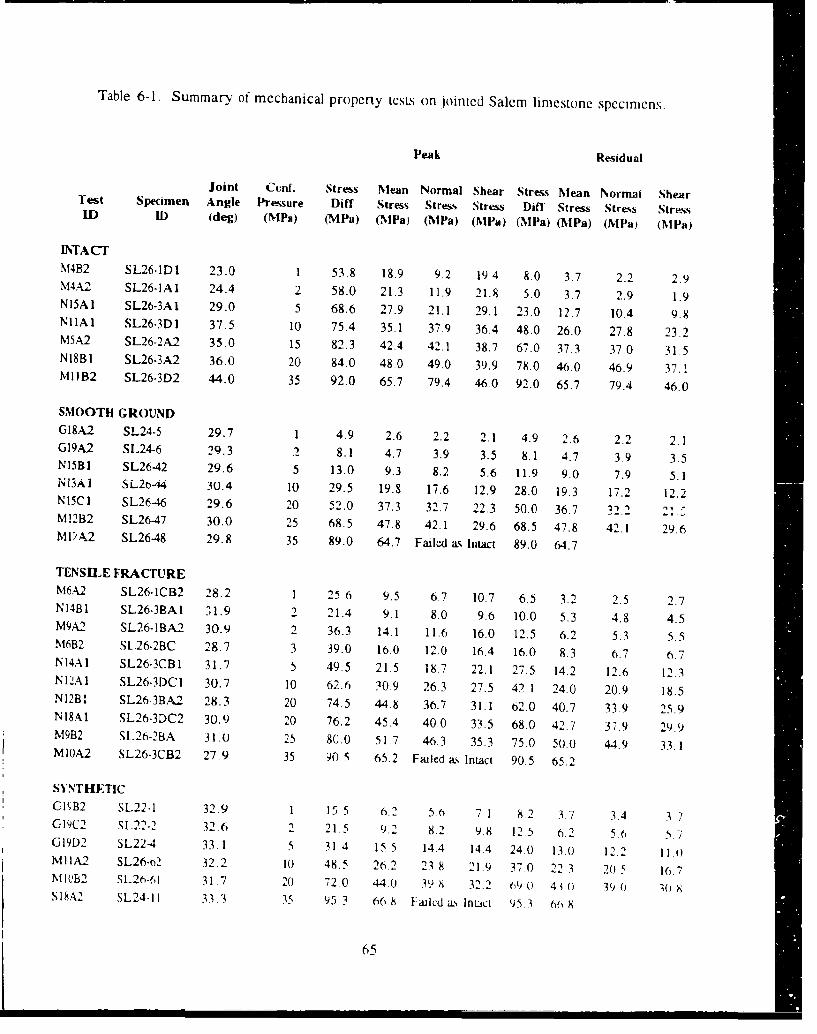
Table 6-1. Summary of mechanical property tests on jointed Salem limestone spcciniens.

Peak Residual

Joint Conf. Stress Nlean Normal Shear Stress Mean Normal ShearTest Specimen Angle Pressure Diff Stress Stress Stress Dift Stress Stress StressII) ID (deg) (MPa) (MPa) (MiPa) (MPa) (NiPa) (IaPa) (MPa) (MPa) (MPa)

INTACTM4B2 SL26-1D1 23.0 1 53.8 18.9 9.2 19.4 8.0 3.7 2.2 2.9M4A2 SL26-1A 1 24.4 2 58.0 21.3 11.9 21.8 5.0 3.7 2.9 1.9NISAI SL26-3A 1 29.0 5 68.6 27.9 21.1 29.1 23.0 12 7 10.4 9.8NI1A1 SL26-3D1 37.5 10 75.4 35.1 37.9 36.4 48.0 26.0 27.8 23.2MSA2 SL26-2A2 35.0 15 82.3 42.4 42.1 38.7 67.0 37.3 37.0 31.5NI8BI SL26-3A.2 36.0 20 84.0 48.0 49.0 39.9 78.0 46.0 46.9 37.!MIIB2 SL26-3D2 44.0 35 92.0 65.7 79.4 46.0 92.0 65.7 79.4 46.0

SMOOTH GROUNDG18A2 SL24-5 29.7 1 4.9 2.6 2.2 2.1 4.9 2.6 2.2 2.1G19A2 SL24-6 2c.3 2 8.1 4.7 3.9 3.5 8.1 4.7 3.9 3.5NI5BI SL26-42 29.6 5 13.0 9.3 8.2 5.6 11.9 9.0 7.9 5.1NI3AI SL2ot-44 30.4 10 29.5 19.8 17.6 12.9 28.0 19.3 17.2 12.2N15CI SL26-46 29.6 20 52.0 37.3 32.7 22.3 50.0 36.7 32.2 21.3M1212 SL26-47 30.0 25 68.5 47.8 42.1 29.6 68.5 47.8 42.1 29.6M I1I'A 2 SL2648 29.8 35 89.0 64.7 Failed as Intact 89.0 64.7

TENSILE FRACTUREM6A2 SL26-ICB2 28.2 1 25 6 9.5 6.7 10.7 6.5 3.2 2.5 2.7NI4BI SL26-3BAI 31.9 2 21.4 9.1 8.0 9.6 10.0 5.3 4.8 4.5M9A2 SL26-1BA2 30.9 2 36.3 14.1 11.6 16.0 12.5 6.2 5.3 5.5M6B2 SL.26-2BC 28.7 3 39.0 16.0 12.0 16.4 16.0 8.3 6.7 6.7N•4AI SL26-3CB1 31.7 5 49.5 21.5 187 22.1 27.5 14.2 12.6 12.3N12AI SL26-3DCI 30.7 10 62.6 30.9 26.3 27.5 42.1 24.0 20.9 18.5N12BI SL26-3BA2 28.3 20 74.5 44.8 36.7 31.1 62.0 40.7 33.9 25.9NI8A1 SL26-3DC2 30.9 20 76.2 45.4 40.0 33.5 68.0 42.7 37.9 29.9M9B2 S1.26.2BA 31.0 25 80.0 51.7 46.3 35.3 75.0 50.0 44.9 33.1MIOA2 SL26-3CB2 27.9 35 ý0.5 65.2 Faled as Intact 90.5 65.2

SYNThITICCMI2 SL22-1 32.9 1 15 5 2 56 7 1 82 3.7 3.4 37G19C2 SL22-2 32.6 2 21.5 9.2 8.2 9.8 12.5 6.2 5.6 5,7G19D2 SL22-4 33.1 5 31.4 15.5 14.4 14.4 24.0 13.0 12.2 11.0N1 IIA-2 SL26-62 32.2 10 48.5 26.2 23 8 21.9 37.0 22 3 20.5 16.7IMIOB2 SL26-61 31.7 20 72.0 44.0 39.8 32.2 69 0 41 (0 3Y0 1( 8S18A2 SL24-11 33 3 35 95.3 66.8 •:1lcd ais Inuct 95. 61 8

65

CýC

ciii

CQ

U

L.I

'I,

C 04

C5*~

L U

• .

00

0000 0) Cý Icot

('CdW) ac3U@.xJJ!G s SSJI

66

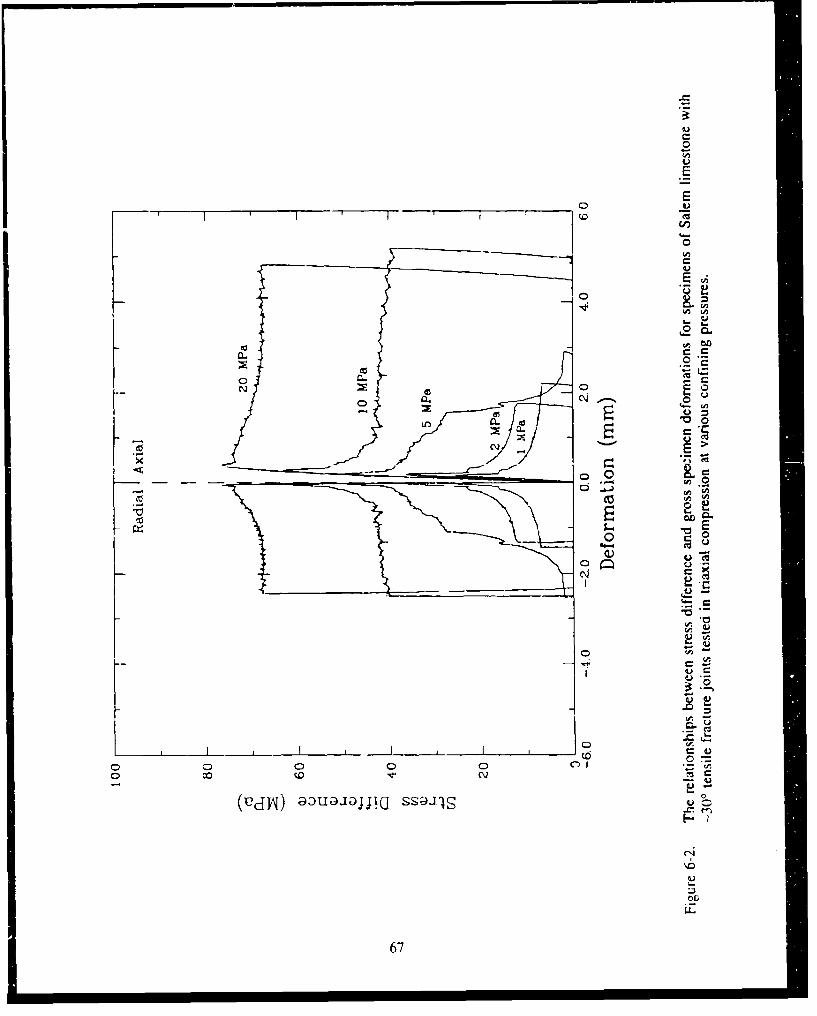
EU

0C U

c

I-v

CA

K 1!CO, b • .

a.U CU

' W5

15

0 C--'

co CD

67

IC _ _ _ _ _ _I

EE

CdE

C-C

o

oC

H °-o c

• ,a~a

o N0

.68

o 0 0 a 0 I-- 1

(•dBN) acuaanJJTIQ ssaal$J,•

688

f...•f-e%•8

"a E

S°o

oI ... • • u

• C I= • --0 "r"

• ,• i.J

•mo•"• 0

, .•.•_ __

I ,1, •7

o o c o o o •.= =

(•dBI) eouoa•jjT(] ssoa•S

.f.

69

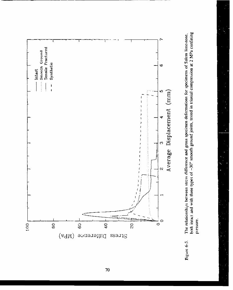
C.2

t'0 0=

COj

IoiOfKt E~

.0 C

70I

o coc

I-

~~V '. ,D/I'----

-008

©" (d) Iu -t,• sa•

to

0 co

71--

II !1III I I I I I II II @I ls

_ _ _ _ _ _•__ _ _-_ _:-__ ____I-I I I I b •

E M

TK8

E 2

0E

-•-. -.

0 CQ

,,¢ -. " .=

SI ,d IN , I "1 "1'S

722

o o oo o o"E.2

I I. i I

L I i --

r1 .. -. ... .._-

I- I • , -i .,z- .

I . .. •- -

73 -

• - .__ _ __ . ,-_- -I._

I ,-•

-- - . I( _ ;

_ -..-- _ I -

, _ , -

(•c•") •o • !(-ss l

I- I

IQ_

74C

Lz

-"2

_ In

---

(12dW)~~~. --l- 11aI

75.....

... -.C)

--\] --

s J*sLJ 0 0 L<).-

I I ! I , ___._O_ _ •• -

75

I/--,-

r I

.,-.4

VV

0 Q)

•.--"-, 0Lo .1 (

.-- • ,/2 (J

-"Ic'- I \

03 0 <f x ' ,

E1.

76

I -.2 -•

•-- '• -I~ -•

VI -• . =S C\2 t 0 "

Ln , o N 1 • . ' L• .

(edll) ss~aJS ta~qS IluIof

I ., -

I i

0I ... j - -

0

S2.

CDC

SI,!I .. L...

(P, AJ,), ss aP S. V11-u-oN luluf .,,-

77

_ _ _ _ _ _ _ _ _ _ _ _ _ _ _ _ _ _ _'

'160

-I

xP

"I 2

(L'dW) SsII P@4 u

w -I "' .- -

( "/ I

, / . I -..

"I - - ' - / -=o0 1 I ,' ,

I. /. 1 ,.

_ _ .. }.o-- ' •-."-

o o 0 0 c - ,

Z-

I C) 0

(1dY ssolj 1LUON °o78/

-0=

\ o ,"

-!-

i "";

(-d}•) - =SI~~N•uo'L

"78

I. ISI -

C00

I- - -- "

L zI

,,I -=

V"Oj

CA

L- I"0• L'

/ --.- I ,I

- . I - "--

IF 2 5i.... '

wa

0l 020

(QdY0~~~~ ss,-II 11u.INlu

I '

4- 0

" ° "1 .. I

¢. 000 U 0 ,(eN)ss--~.zo C-,o

- ,IK -- -~-----~--------79

ZnI

"--

CC

-1P

c Li i

WI -1 =

I I .

-i i --

I_ I I=

SI --3

(tUrn) -1u eapp

ds T(j IetU.tON -u~or

80-

I --

K 80

I.-

CDC

C-

I I "-" T

/ '- -

V H

/I'./ -:= = •.

iI / • -

_ _ _ _ _ _ _------.I

(uiui) :•u~a3ao¶IsT(] TUCUJoN ]uIof c

8,

, ^

;tz

. a.

i

CD

C

I

I •

I -

II

I

*'--

I a Ii N - - -

II -.

I -

I.-

I'

"'="

I L

(

)-

CL; '-L

I2I

-'

I..

82

SECTION 7

EFFECTS OF VARIATIONS IN DEFORMATION RATE

This section descnbes a series of tests that was performed to investigate the influence of

deformation rate on the strength of Salem limestone as measured in triaxial compression tests.

Tests were performed at strain rates ranging from 10s to 102 s-' on specimens of both intact and

jointed limestone, and tests were performed on both damp (2.5 % water content) specimens and

specimens which were fully saturated and then allowed to drain during loading. This section

documents the results of those tests as well as a series of numerical simulations of the tests on

intact specimens.

7.1 STRAIN RATE TESTS ON INTACT SALEM LIMESTONE.

For the purpose of investigating the dependence on strain rate of the strength and

deformation properties cf th- limestone, triaxial compression tests were performed, as described

in Section 4.3.1, at 20 MPa confining pressure on intact specimens of Salem limestone at strain

rates of 10' and 10"i s'. One set of tests was performed on limestone that was damp, but not

saturated (2.5 % water content), and a companion set was performed on specimens that were

fully saturated, but allowed to drain during testing. In addition to those two rates, a 20-MPa

test was performed on an unsaturated specimen at 10' s' as part of the joint strength and

deformation study described in Section 6. Lubricating materials were used between the

specimen ends and the steel endcaps in all tests. In the saturated drained tests, drainage was

allowed through a single 1.6-r&m diameter hole in the lubricating membranes and the solid steel

base cap. Figure 7-1 presents the measured stress difference as a function of axial strain for the

unsaturated tests. The corresponding data for the saturated drained tests are shown in Figure

7-2.

In addition to the 20-MPa tests described in the preceding paragraph, a similar set of tests

was perfcrned on specimens of damp (unsaturated) Salem limestone at 25 MPa confining

pressure with loading at rates of 100, I10, 10', and 10.2 s'. The stress-strain curves from those

tests are presented in Figure 7-3. No saturated drained tests were performed at 25 MPa

confining pressure.

83

The peak Stresses re,.orded in all three test senes are plotted against strain rate in Figure

7-4. The plot illustrates a clear dependence of strength on strain rate in all three cases. In

unsaturated tests, the strength increases approximately 5% per decade increase in strain rate.

As shown in Figure 7-4, the limestone exhibited strengths approximately 5% lower in

the saturated drained condition than when tested damp but not saturated. One possible

explanation for this is that there was insufficient drainage to prevent the build-up of pore

pressure in the specimen. If significant pore pressure did develop, the resulting decrease in

effective stress could cause the observed decrease in strength. The only pore pressure

measurement made during the test was at the base of the specimen adjacent to the drain port.

No significant pressure was measured there. However, that does not preclude the possibility of

elevated pore pressure at locations more distant from the drain port.

7.1.1 Numerical Simulations or Intact Tests.

In oy '-r to assess the possibility that the reduction in strength observed in the saturated

drained tests was a result of pore pressure developed in the specimen at locations distant from

the drain port, numerical simulations of the saturated drained tests were performed. The

simulations were run using the Material Element Model (MEM) program (Chitty, et al. 1993).

MEM is a special-purpose finite element code developed to support material modeling of fully

or partially saturated porous materials, including fluid transport. It implements a fully coupled

compressibility model, which is based on the effec .ve stress concept. This model includes

independent constitutive relationships for the porous skeleton, the solid grains, amid the pore

fluid, and enforces the compatibility relationships among all the materials. It can simulate

arbitrary skeleton boundary conditions specified in terms of either stress or deformation, as well

as various fluid flow conditions.

As shown by the triaxial compression test data presented in Figure 7-1, the Salem

limestone at 20 MPa confinement exhibits brittle response. That is, the axial stress reaches a

peak and then decreases with additional axial deformation, a phenomenon sometimes called

strain softening. Since none of the available nonlinear skeleton constitutive models were

8€

capable of modeling that behavior, a linear skeleton model was used to simulate the pre-failure

portions of the tests. The test data presented in Figure 7-5 show that the limestone is suffer

when loaded at the rate of 101 s' than when loaded at the lower rate of 10-' s This ;s due to

the time-dependent behavior of the rock skeleton. A significant body of literature exists on the

subject of time-dependent behavior of geologic materials. Sun (1986) and Hardy and Sun (1986)

developed a nonlinear constitutive relation to describe this phenomenon. Although the overall

compliance of the rock specimen is a complex combination of the elasticity, plasticity, and

viscosity of the rock, it can be described by a constant rodulus or apparent modulus •t a

particular load rate. Based on the results of the unsaturated tests presented in Figure 7-5, elastic

bulk moduli of 13,000 MPa and 17,500 MPa were selected to model the response of the porous

Salem limestone skeleton loaded at lOr s' and 10' s', respectively. In both cases, a Poisson's

ratio of 0.25 was used.

The simulations of the saturated drained tests were performed using the axisyrrmetricSj.i ine ^t ..... L- -i'--

liniurc.,.,,•, msm sw,• in Figure 7-6. On one end of the specimen, drrinage was allowed

through the on-axis node and the next closest node to simulate the drain port in the actual

experiment. Based on the measurements reported in Section 9, the permeability of the limestone

was set to 2 x 10'i m2. This value is slightly lower than the permeability observed for the

Salem limestone at the highest mean stress (approx. 50 MPa) reached in the 20 MPa triaxial

compression test being simulated. It was chosen to accentuate any possible effect of poor

drainage and saturation of the test specimens. Since lubricated endcaps were used in all of the

tests, the radial degrees of freedom were rot constrained at the specimen ends. In the axial

direction, a displacement boundary condition was specified with the peak displacement

corresponding to the actual peak displacement during tLLe test being simulated. The 20-MPa

confining pressure was applied radially.

Figures 7-7 and 7-8 show comparisons of the numerical predictions by MEM and the test

data. As expected, the linear elastic skeleton properties derived from the unsaturated tests result

in reasonable agreement between the saturated drained test data and the multi-phase numerical

simulations, although the measured stress-strain curve for the saturated drained test at the slow

(10' s-') strain rate is not as linear as those from the other tests. Figures 7-7 and 7-8 also show

,035

the pore pressures computed by rte simulations for the ends of the soeimens away from the

drain port. In the slow (10-' s') strain rate case, no Lignificant pore pressure developed in the

simulation, and the cvjrve is barely visible at the bottom of the plot. In the simulation of #he

faster (10-' .') strain rate test, the pore pressure away from the drain increawd to 4 MPa and

remained there for the remainder of the simulation. Because of the value of permeability

selected for the simulation, this represents an upper bound on tJhe pore pressure that would be

expected to develop in the actual test. If 4 MPa of pore pressure did develop, then the c-ffective

normal stress on the rock skeleton would be reduced by that amount and the strength exhibited

by the material in the test would be lower. To estimate how much lower, consider the strength

envelope in Figure 5.6. In that figure, the strength developed by the specimen tested at 15 MPa

confining pressure was about 2 MPa lower than the corresponding value for tOe 20 MPa test.

This does not account for the fact that the unsaturated specimen reached a strength 5 MPA higher

than the saturated drained specimen. A similar conclusion can be drawn fo! the case of the

lower strain rate. While the simulation results suggest that no significant pore pre.,ure was10 ... .. M` 1 "U C"S- - + t - 4 N nIC

l ihe t u 1t--ain. sp1cU i,, at 3hV IF sstrain rLe, ,,,. IV 3 S Ma le4s

than that of the unsaturated specimen loaded at the same rate.

It appears that some factor that is not treated in the current test and analysis techniques

is responsible for th- difference in strength between the unsaturated and saturated drained tests.

This could possibly be a chemical interaction, similar to the phenomenon that results in higher

strengths in oven dried unconfined compression tests than in damp tests. Alternatively, it could

possibly result from saturationi and reduction of effective stress on a microscopic level in dead-

end pores which are not adequately rpresented by the permeabiTty tests.

7.2 STRAIN RATE TESTS ON JOINTED SALEM LLMUFSTONE.

Triaxial compressioai tests were also performcd on limestone specimens comnaining joints

of the three types aeicribed in Section 3 oriented at 30' to the axes of the specimens. As with

the tests on intact rock described in the previous subsection, tests were performed on specimens

that were both damp and saturated drained. The stress-deformation curves for the tensile

fracture, smooth ground, and synt-ietic joints are presented in Figures 7-9 through 7- 11,

86

respectively. Due to slight differences in joint angle, it is not possible to make direct

comparisons among the maximum values of stress difference reached by the varnous tests. A

more meaningful comparison is can be made on the strength plots presented in Figures 7-12

through 7-14 for the three joint types. Shown for comparison in each figure is the strength

envelope reported in Section 6 for the corresponding joint type tested at a strain rate of 10-' s-'.

The strengths for tensile fracture joints are shown in Figure 7-12. The higher strain rate

(10. s") tests in beth saturated drained and unsaturated tests exhibited strengths approximately

5 % higher than the corresponding points in the strength envelope derived from tests conducted

at 10"' s'*, and relative to the strength envelope, there is essentially no difference between the

saturated drained and unsaturated tests. At the lower strain rate (10" s'), the unsaturated

strength is virtually the same as the envelope for 10 s' envelope and the saturated drained

st.rength falls approximately 5% below the envelope. Overall, there appears to be a strain rate

effect of similar maugnitude to the intact material, but the initial saturation does not appear to

significantly influence the result of a test in this configuration. A jointed specimen tested under

saturated drained conditions is probably less likely to develop pore pressure in a 20-MPa triaxial

compression test than an intact specimen tested under the same conditions. Although the joints

compact slightly while shearing at this confining pressure, the sliding of the two halves of the

joint tends to create small gaps where the joint intersects the jacket that actually increase the

volume available for the pore water to occupy, and thus minimize the chance of development

of any significant pore pressure in the specimen.

The tests on smooth ground joints, for which strengths are shown in Figure 7-13, all fall

very close to the original strength envelope from the tests conducted at 10' s". Only the

saturated drained test data point lies slightly above the envelope. However, based on the small

number of data points, the difference is insignificant. The conclusion from this limited study

is that neither sarain rate within the range studied, nor initial saturation significantly affects the

strength of smooth ground joints.

The results of tests on synthetic joints are presented in Figure 7-14. As with the smooth

ground joints, cnly one of the four points deviates from the original fit line. In contrast to the

87

smooth ground tests, it is a higi:i su-ain rate test which falls slightly below the envelope. Since

the deviation is very small and in the opposite direction from the trends exhibited by the intact

and tensile fracture jointed specimens, it is considered to be natural scatter. As with the smooth

ground joints, it is concluded that neither strain rate within the range tested nor initial saturation

significantly affect the strength of the synthetic joints.

88

[ 'I ="

. 0I ( E*1I- * *.- "-

C4

-I -- - - -f

.. ........ •

C4

• -

D CD• •

*I° --

oo N O.

(PdI^;l) 9;Du@.'aJ;IC. ss@aIlc, CE

89

I 1 0

/ V2

'c5 --

I---

04'

I I I II *IIS I I II II II I~900

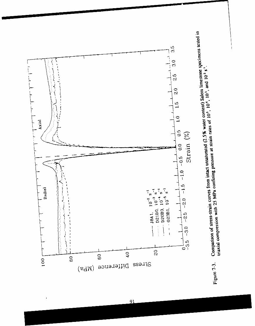
C~C

U-)

~~U,

CNJ 4A

C)K

1.0 t

4 0CrO

co-I h

liaI(12dW)

mo

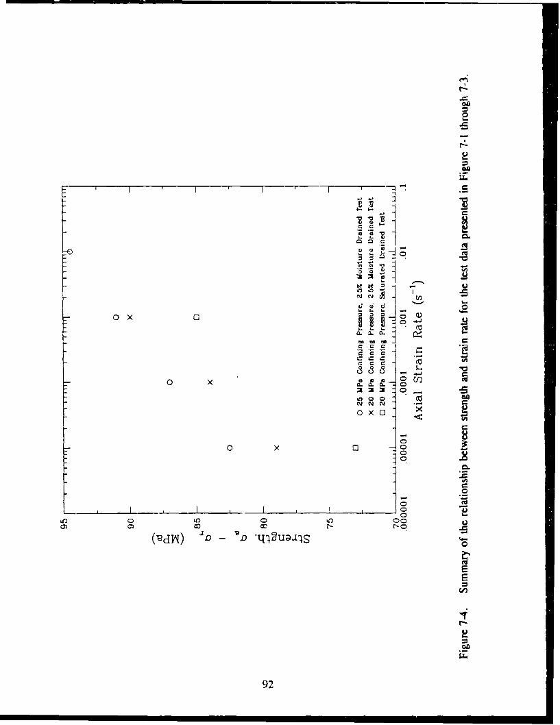
100

i~~~A ý1" ,.0.• .iI

"S

0 x00

-I

1! "-

O 00

- '4-

° -

0 0 .5

Souooe 0 00

92

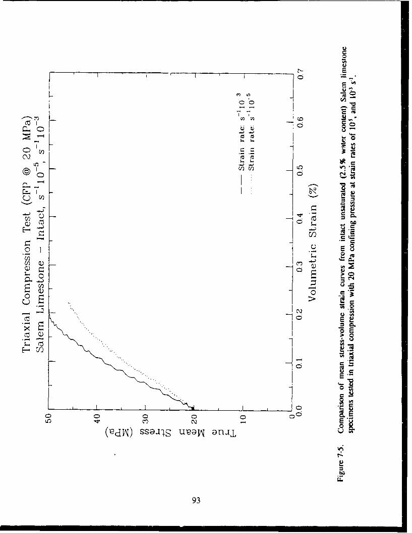
r-- E

CDO 0 '0-.

I....-

Q- J

.2' -' I

o/ I E

0d0 .. ,,

V~)

•- - , .

O) 0 0

CC\2

(CedvW) ss@-II U~Pa @n-IL

93

CLC

EC~C

x0

CIO 0

"" E

CL 0

r) -

E '_ II __ "a) -_lo- ]--- -"*

I-__ L '- "

oI "- "--- - v --

II -I J I I I I....

o~0

CO QQ

c U

t4 Cc

• T S

Loa CLI

94

CD.

LO E

C\2

co,

C\2 VC\2

< I •

r4

I I

ocfA

Q . -- o4

-'IH. d ,II-

-0 0

('2dN) ssC-qS u'-4 Gni

95

I L.n

C\22

rn&

co

<C6

LI --. L - C-8

I:2

ji

OiNh Is-1S UIINGI

5 - I.-o•'

L,-

96

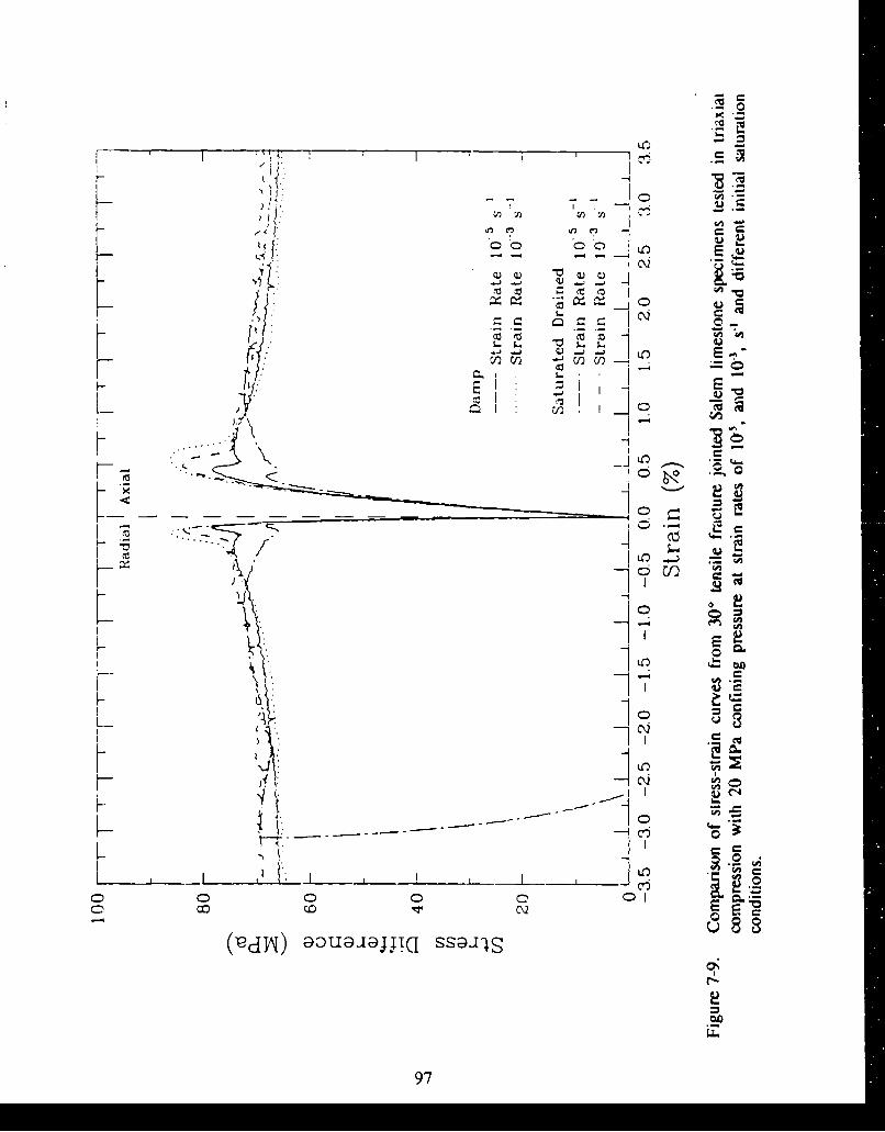
6.J

I " oI

I "

Cd) C ) , C\2-

00 0

"4

-- I

u C.

Q 3

h <.... K---1-

F --v

10

(edvW) Gou@a9JJICi ss~a-S

97

•(

C/) ', ,

I o 0

CO ,,,,,=

I/ III :;

if)C1I'-

• C4

0 C) _C iC.

L I i I I . i - -

4 0 E

98

a i ~ I I I II

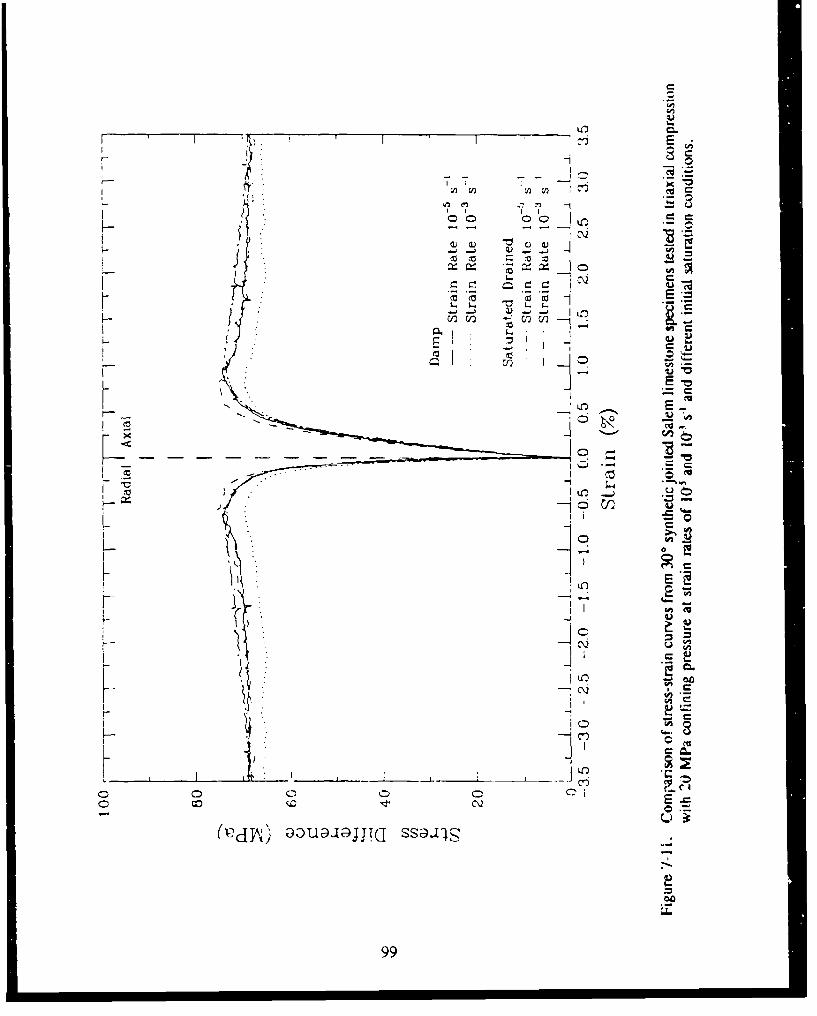
L,

SI•, , l lI I II.,

co -Z _utK- T - - - -_ .

d I I I I

99oU,'--.'{ 1 "*

-I '-I, I. " '

FL

i §, -J--o

I a!

K- '4'i0

I ___ ___ ___ ___

o 0 0 0 0 -

99

7.9,

0_ _ _ _ 0

-1- C,

0 --

'L =-4'--

v2.

\0ir

II *1 " "-

- - - . .

I-- " -

•2 I(.3

1 m C !00

..

c

cd 0

K-.-

?LL

oO

101

I .I

I -

2

I- -

L 20

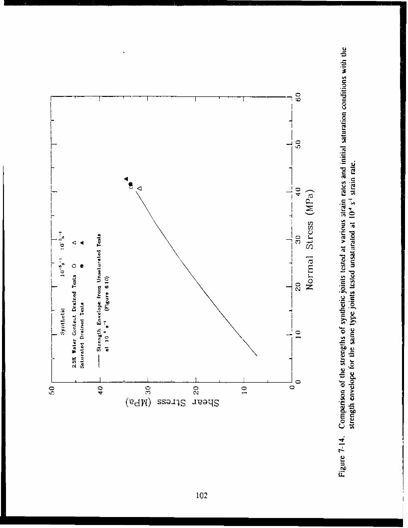
,'5

I'"- ' I 1 I •=€

r

h2 S

E I

B C-'

, 10

1- .2

I I _ -

I I 0 U,

•, . I ,iI .

o• -

(cdv4) ssa.xS xe•is

102

SECTION 8

SATURATED UNDRAINED HYDROSTATIC COMPRESSION TEST

AND SPECIFIC STORAGE MEASUREMENT

A series of saturated undrained hydrostatic compression tests were performed to

determine the ratio between induced pore pressure and imposed hydrostatic stress, and to

evaluate the specific storage of saturated Salem Limestone. This section describes those tests

and presents an analysis of the results.

8.1 TEST PROCEDURES.

These tests were performed on intact specimens prepared with a polyolefin jacket as

described in Section 4. 1. They were instrumented with axial and radial LVDTs and strain gages

as described in Section 4.4, and saturated with water as described in Section 4.2.2. In addition

to the usalW complement of instrumentation, a gage was installed to measure the volume of pore

fluid drained from the specimen. It consisted of a small (approx. 20-mm diameter) hydraulic

cylinder with an LVDT installed that measured displacement of the piston relative to the

cylinder. It was plumbed into the pore pressure drain line in such a way that it could be

evacuated and saturated with water in a manner similar to the rock specimen. Approximately

0.7 MPa of air pressure was applied to the cylinder on the pore fluid side to prevent any

cavitation.

With the pore pressure drain valve closed, the hydrostatic pressure increased to 137 MPa

(20,000 psi). The pore pressure drain valve in the basecap directly beneath the test specimen

was then opened slightly allowing the pore pressure in the specimen to slowly diminish, while

monitoring the pore pressure with the pore pressure transducer, also located in the specimen's

basecap. During each test, volume of pore water draining from the specimen during this

consolidation process was measured using the volumetric device described above.

103

L

8.2 TEST RESUILTS.

There were five specimens tested in this manner. Typical results are shown in Figures

8-1 through 8-3. Figure 8-1 presents the hydrostatic confining pressure (total stress), pore

pressure, and effective stress changing with volumetric strain. Through the entire initial loading

phase of the test, the rock skeleton remains elastic, and the total stress is approximately equally

divided between the pore fluid and the rock skeleton (effective stress). When the confining

pressure reached the piedetermined value of 138 MPa, the volumetric straiii in the specimen was

approximately 0.7%. At that point, the confining pressure was held constant while the excess

pore fluid was ilowly drained. As the pore pressure dropped, the effective stress increased,

until it equalled the confining pressi,re. In Figuie 8-2, radial strain is plotted against axial

strain. The anisotropy in the rock skeleton illustrated in Figure 8-2 is consistent with the

drained hydrosta'kc compression test data presented in Figure 5-8. Figure 8-3 shows the tota!

amount of water expelled from the specimen as a function of the instanta"e.,y pore pressure

inside the specimen. The drainage of pore pres-sure depicted in Figure 8 -, c4-urred over a

period of approximately 20 minutes.

8.3 RATIO BETWEEN PORE PRESSURE AND HYDROSTATIC STRESS.

The ratio between the induced pore pressure and the imposed hydrostatic stress depends

on the compressibility properties of the materials involved. Based on the fully coupled

compressibility model presented by Blouin and Kim (1984), the total strain in a fully saturated

rock in hydrostatic compression can, be viewed as either the sum of the strain in the grain/water

mixture under pore pressure, ir, plus that of the solid grains caused by effective stress, P, or

as the sum of the strain in the skeleton due to effective stress plus the strain in the grains under

pore pressure. Setting both of these expressions equal, since they are descriptions of the same

total strain in different ways, gives:

+ P M = + I+ (8.1)K. K, K, K4

in which K, is the grain bulk modulus of the rock, K, is the bulk modulus of the skeleton, and

K. is the bulk modulus of the water/grain mixture, which is expressed as:

. 4-

K, = (8.2)K.= . + r. (KS- K.) .)

where K, is the bulk modulus of water and n is porosity of the rock. From Equation (8.1), the

relation between pore pressure. and effective stress can be obtained:

o -- ,9 . (8.3)K, (Ks K)

Since the total hydrostatic stress or confining pressure, P=P +•, the ratio between pore pressure

and hydrostatic stress can be found by:

"- .. ! 11 = (8.4)P- + 71

Equations 8.3 and 8.4 define, theoretically, the ratio of pore pressure to total

(hydrostatic) stress. Published values for the bulk moduli of water and solid calcium carbonate

are, respectively, K.,=2260 MPa, K,=82000 MPa. For the Salem limestone used as a test

specimen, n=0.169, and K,= 14085 MPa (from the data presented in Section 5). Substituting

these values into Equations 8.3 and 8.4, it can be found that #= 1.237 and the ratio of pore

pressure to total stress, T/P, is 0.447.

The computation of the pressure ratio in the preceding paragraph was based on the

assumption of constant linear bulk moduli for all constituent materials. A more detailed

simulation, based on nonlinear pressure-volume strain relationships, was also performed using

a version of the program NKOCP (Kim, Blouin, and Timian, 1986) that was modified to include

a grain compressibility model for calcium carbonate based on test data specific to that mineral.

It also includes a nonlinear compressibility formulation for water. In addition to the pore fluid

and grain compressibility models, this program requires input of the rock skeleton

compizssibility hi the form of a pressure-volume strain curve from a drained hydrosta-.

compression test on the material of interest. For this calculation, the test data shown in Figure

5-7 were used to define the skeleton compressibility. NKOCP numerically integrates along the

105

skeleton compressibility curve using the fully coupled formulation, which maintains full strain

compatibility, to calculate the response of the material in the saturated undrained condition.

Figure 8-4 presents comparisons between the stresses measured in a saturated undrained

hydrostatic compression test and those calculated using NKOCP with input from a drained

hyd'ostatic compression test on the same material. Total stress, effective stress, and pore

pressure ar: compared independcrnly in the figure. There is very good agreement between the

test data and the numerical simulations which are based on the effective stress approach. Figure

8-5 shows the ratio of pore pressure to total confining pressure computed by the NKOCP

simulation and compared with the results of two saturated undrmined tests. Again, the agreement

is very good, especially considering that this presentation tends to exaggerate small differences.

Laboratory experience showed that the ratio of pore to confining pressure will eventually

converge to the same level with increasing hydrostatic stress, regardless of ,he initial pressure

ratio imposed at the beginning of the test. In order to provide a theoretical rationale for this

phenomenon, additional numerical simulations were conducted with NKOCP using different

initial conditions of pore to confining pressure ratio. The results are plotted in Figure 8-6, with

initial pressure ratios of 0.2, 0.4, and 0.6. This plot confirms the convergence of the pore to

hydrostatic pressure ratio with increasing hydrostatic pressure, as observed in laboratory.

Furthermore, the simulations show the dependance on the initial pre. :;ur, ratio at the beginning

of the experiment.

8.4 SPECIFIC STORAGE.

Most standard methods for specific storage measurement, such as those from ASTM,

NGWA, apply to field tests on underground aquifers. The specific storage of a saturated aquifer

is defined as the volume of water that a unit volume of aquifer releases from storage under a

unit decline in hydraulic head (Freeze and Cherry, 1979). In a laboratory test, the aquifer

referred to in this definition is ;.he rock specimen under study. Based on this definition, the

following formula was developed for derivation of specific storage from the laboratory data

described in Section 8.2:

106

So v,,- vw, (8.5)

where S, is the specific storage of the rock specimen, V, is the total volume of the specimen, V,,

is the measurement of the volume of pore fluid drained from the rock specimen, i is the pore

pressure. V,,, and r, are the drained water volume and pore pressure measurements,

respectively, at point a, where the specific storage measurement is started. For the calculation

presented here, the point a was selected as the point of maximum pore pressure at which the

drainage port was opened in the experiment. This is illustrated in Figure 8-3, where the specific

storage is the negative of the slope of the curve, normalized by the volume of the specimen.

In order to eliminate the noise that would result from performing an instantaneous numerical

differentiation on the data in Figure 8-3, the specific storage curves were derived from the test

data by taking successive secant slopes, all beginning with the starting point a. Those specific

storage results for the Salem limestone specimens, which have values ranging from 1.4 to 2.8

xlOW MPa-1 , are plotted in Figure 8-7 against the effective stress on the rock specimen.

From an analytical point of view, the total volume of water expelled from the rock

specimen, AV., can be considered as two parts. The first part, AV,,,, is the pore water

expansion caused by decline of pore pressure, which can be expressed as:

A V.,, 1 A a V, (8.6)K.,

where n is porosity, K, is the bulk modulus of pore water. Because of the decline of pore

pressure, AT, the effective stress a. increases. The increment, Ao,', will further squeeze the rock

skeleton and reduce its pore volume. This volume reduction will expel an equal amount of

water from the specimen, which constitutes the second part, AV,2. According to the fully

coupled compressibility model (Blouin and Kim, 1984):

a 7t10 7 t (8.7)

107

where K, and KC are bulk moduli of the rock skeleton and solid grains, respectively. Then the

total volume of water expelled from the specimen is:

AV,, •V~,, +AV~,,2 = - (8.8)A4 . - 4 V 1 + 4 V 2 = (n -. . . . _-c)v, (8.8)K. K, Ks

Since the total hydrostatic load is unchanged as the water drains, A* =-Ar. According to the

definition given by Equation 8.5, the specific storage is given by:

S, -n I + (8.9)K, Ks Ks

Equation 8.9 is an expression for specific storage in terms material properties. Taking the bulk

moduli of the grains and water as constants (82000 MIPa and 2260 MPa, respectively), and using

the hydrostatic test data from Figure 5-7 to define the skeleton bulk modulus, K,, as a function

of effective stress, a simple prediction of specific storage of the limestone is obtained. This

prediction is plotted in Figure 8-7 along with the experimental results.

Comparison of specific storage values from pore fluid drainage volume measurements

with those derived from material properties showed good agreement at the beginning part of the

experiment, where the pore pressure was highest. The measured responses diverge from the

computed curve at effective stresses above about 75 MPa.

108

0 0

-- e2

00

--.

r.2

-J ~ -:

0' 0.....'•=0

(0dvj) GlJnssl-d

109

LIIII ,...

L i -

J0

ce,

co C\2

L

dV

110

I.

i-1 I.-.

Ii0

I I--

- 2-.- -

0 U.

111

I I I II I o I~

200 , I i

I.I.Measured•' ;50 - " "

S......... ComFuted

° _1StOO SI

.,: .•j>>200 J , , I , -

S150 -

S•oo '-

S..- '1:)-": .. .- ' ...... i

S5G ',-..,-. 2oo "• I i

•! 150 -

SI00 - /

S' • I•- 50 ,.-- •"

0 • r-''• , • ' I

0 2. .4 .6 8

Volume Strain (•)

Figure 8-4 Comparison between the results of a saturated undrained hydrostaticcompression test on Salem limestone with a numerical simulation based ondrained rock skeleton properties.

112

-, IIlQ

c .6.2

I

L•

, 0 0

j o --

- • V

1V V i s0

ic" I -.

I "I-

113U

• -II II II 0_

C a.Io

a4. 1. CL. I-

-I '..

K0

.,1" U2 U

1 4 --

I 000' -•--

~0 0

. L. I•

"I -...- ,

K114

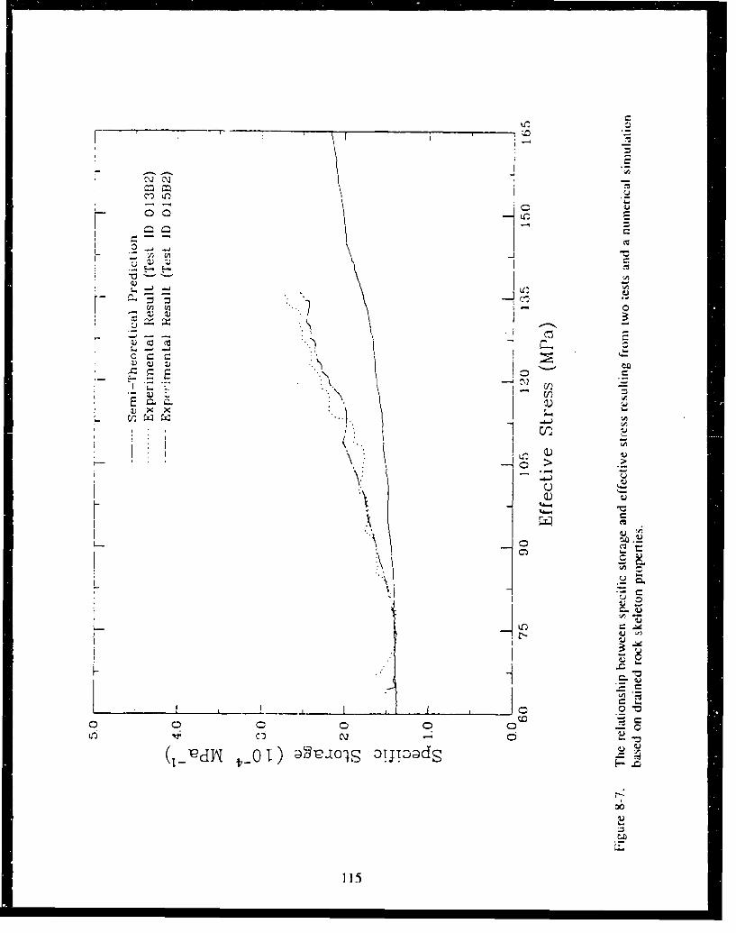
'7S

. I"-

oo- --=4 m

I- ° - - *-*

I H

X X~L

.. I .- I " -f,"-

* .. .. -\ I" n -

* LI

V U=t ~~c cvxx: '-- j,_" ' I "1 "I

215

I_ ,. C

1 , • ., . .o "

.-:

115

SECTION 9

PERMEABILITY OF INTACT AND JOWITED LIMESTONE

A series of laboratory tests was performed to measure fluid flow through intact and

jointed Salem limestone specimens under a wide range of stress conditions. The objectives of

this effort were to measure the permeability properties of the intact rock and rock juints and to

correlate these properties with the mechanical response of the rock.

For intact specimens, permeability tests were first conducted under hydrostatic loadings

over a range of pressures, and an empirical relationship between permeability and hydrostatic

stress was developed. Then permeability was measured for the limestone specimens under

different triaxial stress conditions with confining pressures ranging from 5 to 90 MPa. Based

on the empirical relationship for hydrostatic loading, a component of permeability related to the

deviatoric deformation was identified. An empirical model relating permeability and mechanical

response was developed for Salem limestone.

Fluid flow tests under a range of hydrostatic stress conditions were performed on the

three different types of joint surfaces described in Section 3: tensile fractures, smooth ground

surfaces, and synthetic joints consisting of mating surfaces produced on a numerically controlled

milling machine. Comparisons were made between the measured flows through intact and

jointed specimens, and the results used to develop empirical models relating permeability of the

different joint types to joint normal stress.

9.1 DESCRIPTION OF EXPERIMENT.

This section describes the equipment and procedures used to perform the hydraulic

permeability tests and presents background on the formulation of flow laws for permeable

materials.

116

9.1.1 Test Specimens, Equipment, and Instrumentation.

The experiments were carried out in a computer controlled triaxial compression apparatus

that had been specially modified to perform fluid flow tests. Figure 9-1 presents a schematic

of the equipment used in these tests. The permeability tests were performed on cylindrical

specimens of Salem limestone approximately 48 mm in diameter and 96 mm long, the same as

those used in the mechanical property tests. For measurements of joint permeability, specimens

were prepared with the three types of joint surfaces described in Section 3. However, the

permeability specimens had the joint oriented parallel to their axis and, ideally, in a plane

containing the axis. Preparation and instrumentation of the permeability test specimens closely

followed the procedures described in Section 4. As in the mechanical property tests, the rock

specimen was installed in the triaxial chamber between upper and lower endcaps and sealed with

a polyolefin jacket. The endcaps had flow conduits, and pore fluid diffusers were placed at each

end between the specimen and the medcap to evenly distribute flow over the ends of the specimen

through a series of equally spaced holes. In order to limit variations in the rock skeleton stress

field, the total cross sectional area of the holes was no more than 10% of the end area of t'

specimen. At the bottom of the specimen, fluid was pumped in through the same port in the

pressure vessel that is used for saturation of porous specimens. At the top, fluid was allowed

to flow out through holes in a specially modified piston in the triaxial apparatus which was

sealed to the specimen endcap by means of an O-ring. The upper endcap was also strain gaged

to serve as a load cell for axial stress measurement. Where deformation instrumentation was

used, it was of the same type as in the mechanical property tests as descried in Section 4.4.

The flow of fluid to the limestone specimen was supplied by an intensifier, i.e. a small

diameter hydraulic cylinder driven by a larger diameter cylinder. By supplying approximately

20 MPa hydraulic fluid pressure to the large diameter side of the intensifier, it was possible .o

generate up to 138 MPa of water pressure on the small diameter side. This is illustrated

schematically in Figure 9-1. The rate of pore fluid flow was controlled by regulating the flow

of hydraulic fluid to the low-pressure side of the intensifier. By installing a displacement

transducer (LVDT) to measure piston displacement, the intensifier also provided a means of

measuring the water flow through the specimen. To determine the flow rate, a least squares fit

117

was made to the constant-velocity portion of the piston displacement time history. The resulting

slope is the piston velocity, VV. The apparent fluid velocity, V,, was then computed as:

V V At (9.1)

where: A - area of the high-pressure end of the intensifier

A. = cross section area of the test specimen

A transducer installed in the bottom end cap of the test specimen was used to measure

the pore fluid prcssure on the upstream end of the rock specimen. On the downstream end (the

top) of the specimen, the fluid drain was open to the atmosphere. The pressure drop between

the end of the rock specimen and the atmosphere was negligible, and a downstream pressure

measurement was not made. The pressure transducer. calibr~aed with zero output indicating

atmospheric pressure. Thus, assuming a constant pressure gr, &'ent along the length of the

specimen, the pressure gradient, G,, was computed as:

T •(9.2)

where: P, = fluid pressure at the upstream end of the test specimen

1, = length of the test specimen = length of flow path

As with the mechanical property tests, measurements made by the active instrumentation

were recorded by a microcomputer-based multi-channel digital data acquisition system.

9.1.2 Test Procedures.

All of the permeability tests were performed using distilled de-aired water as the pore

fluid. In preparation for fluid flow t"csting, the test specimen and water supply system were fully

saturated with water. The triaxial chamber was first pressurized to 1-2 MPa to hold the jacket

tight against the specimen. The specimen and water supply system were sealed from the

atmosphere and evacuated, and water was forced into the specimen with the intensifier.

118

Once the specimen and associated piping were fully saturated, the total stress state for

the particular test was imposed on the specimen using the normal triaxial compression loading

functions. It was always necessary to keep the confining pressure in the triaxial chamber higher

than the upstream pore pressure in the specimen. Failure to do so would result in gaps opening

between the specimen and the jacket, allowing erroneous fluid flow. At each total stress state,

multiple fluid flow tests were conducted, each at a constant pressure gradient. In all cases the

downstream pressure was zero. In a typical test series the upstream pressure ranged from

approximately 1 MPa to 90% of the confining pressure. In each permeability run, the upstream

pressure gradient was held constant for a period of 20 to 100 s while data were recorded. The

durations of the tests were selected to allow time for sufficient intensifier displacement to

provide adequate resolution for pore fluid velocity determination.

9.1.3 Fluid Flow Equations.

In traditional civil engineering, where pressure gradients and the resulting flow velocities

are typically small, problems are almost exclusively formulated using the Darcy flow equation

which assumes a linear relationship between pressure gradient and flow velocity. However, in

weapons effects problems of interest, pore pressure gradients and flow rates can be of sufficient

magnitude that the Darcy equation does not adequately describe the pore fluid response. To

analytically treat the dynamic problems, Kim, et.al. (1988) adopted a more general expression

for pressure gradient which includes a term that is proportional to the square of the fluid velocty

in addition to the linear (Darcy) term, along with inertial terms related to fluid acceleration. The

use of the velocity-squared term was apparently first proposed by Forchheimer (1901), and has

been used in various forms by investigators over the years. Forchheimer's equation, which does

not consider fluid acceleration, has the general form:

dG alt V+bV-2 (9.3)dxa

where: GP = pore pressure gradient in the x direction

V. = apparent fluid velocity in the x direction

a,b = constants which are functions of both skeleton and fluid properties

119

While Forchheimer's equation appears to be virtually unknown in the civil engineering literature,

its use is widespread in chemical engineering, particularly with reference to porous metal filters.

The constants, a and b, in Equation 9. 1 are functions of Lhe properties of both the pore fluid and

the porous medium. If Equation 9.1 is divided through by V,, the result is:

a + b V (9.4)Ve

This represents a linear relationship between V. and G^V.. When the test data are plotted with

G^V on the vertical axis and V. on the horizontal, the slope of the resulting line is the quadratic

coefficient, b, and the intercept with the vertical axis is the linear coefficient, a. This form is

convenient for derivation of the coefficients from test data, but for fundamental understanding

of the physical phenomena, a more useful form of the equation will result if it can be expressed

in terms of constants that are dependent on either fluid or porous medium properties, but not

both. Green and Duwez (1951) argue, based on dimensional analysis, that if the factors

controlling the pressure gradient are assumed to be fluid viscosity, fluid density, a length

characterizing the pore openings, and the apparent fluid velocity, then Fc.,;hheimer's equation

must have the form:

G, - conul --- co (9.5)828

where: = dynamic viscosity of the fluid

,f = mass density of the fluid

6 = unknown length related to pore geometry

If the constants are combined with the unknown pore dimension term, 6, and called a and B,

the resulting expression has the desired separation between quantities dependent on skeleton

properties and those dependent on fluid properties:

G -'- +&- 0 (9.6)

a P

120

The relationship between the two sets of coefficients is:

a (9.7)

b

Here, a has units of length squared and 0 has units of length. A linear approximation to the

Forchheimer equation is the familiar Darcy equation:

G E v -? v. (9.8)Kd k

where: K = absolute permeability (length2)

k = Darcy permeability coefficient (length/time)

g = acceleration of gravity

The absolute permeability, K, in Equation 9.5 has the same form as a in Equation 9.3.

However, it can be numerically different because a quadratic fit to a given data set will yield

a different linear coefficient than a linear fit to the same data. The relationship between the two

permeability measures is:

K kp1 g Pf g (9.9)

k = ._f g

121

9.2 PERMEABILITY OF INTACT SALEM LIMESTONE.

Permeability measurements were made on intact specimens of Salem limestone over a

wide range of pressure gradient and skeleton stress and strain conditions, including hydrostatic

confining pressures up to 150 MPa and pressure gradients up to 1500 MPa/m. Included were

tests in which the rock skeleton was loaded in triaxial compression past failure with axial strains

up to 10%. Tables 9-1 through 9-8 show the test conditions applied to each specimen. Under

each loading condition there was a series of eight to twelve flow tests conducted at different pore

pressure gradients. Figures 9-2 and 9-3 &how typical recordings of upstream pore fluid pressure

and pore fluid intensifier displacement, respectively. As shown in Figure 9-3, piston

displacement was held as a linear function of time. In all cases, the correlation coefficients of

the linear fits to piston displacement were greater than 0.99, showing an almost perfect linear

relation between the variables.

9.2.1 Flow Tests with Hydrostatic Skeleton Loading.

Fluid flow tests were performed on intact specimens of Salem limestone which were

subjected to hydrostatic skeleton loading ranging from 1 MPa to 150 MPa. The results of those

tests are summarized in Tables 9-1 and 9-2. Figure 9-4 presents data from the test described

in Table 9-1 in a format for determination of both the linear and quadratic flow coefficients

described by Equation 9.2, where the sope is b, and the intercept is a. At the lower pressures,

the curves have small, but non-zero slopes. At pressures above about 70 MPa, the lines curve

downward with increasing fluid velocity. We believe this nonlinear response is a result of non-

uniform effective stress in the rock specimen which becomes increasingly significant as the

upstream pore pressure approaches the confining pressure. Under this condition, the effective

stress in the rock skeleton approaches zero. As that happens, the flow resistance of the rock

skeleton becomes more like that in the same rock loaded to a lower confining pressure. In order

to minimize the effect of effective stress variations on flow coefficient determination, fits were

performed on only the lower pressure half of the test records. In fits to the 130- and 150-MPa

confining pressure test data, the data points from the lowest pressure gradient tests were also

omitted because they appear to represent some iritial flow resistance that is not characteristic

122

of the overall tests. The resulting flow coefficients are tabulated in Table 9-1 and shown

graphically in Figures 9-5 and 9-6 for a and b, respectively. As expected, the increasing values

of both a and b with increasing confining pressure correspond to decreased flow. Recommended

empirical fits to the data are also shown on *he figures. The break hi slope of the fits is related

to the onset of pore collapse in the rock skeleton.

While we believe the Forchheimer equation, includin'g the quadratic term, is more

fundamentally correct than the linear Darcy equation for representing flow through porous

media, practicality suggests that a linear approximation be evaluated. Rather than simply setting

the quadratic coefficient to zero, the data were re-fit assuming the linear form. The data shown

in Figure 9-4 are presented in different form in Figure 9-7. Here, the axes are pressure gradient

and apparent fluid velocity, and the absolute permeability coefficient, K. is:

K ,- 9 /(9.10)a'

where: a' = the slope of a linear fit to the data as presented in Figure 9-7

, = dynamic viscosity = 1.002 * 10. MPa*s for water at 20 0C

Figure 9-8 presents the values of absolute permeability determined by combining the data in

Table 9-1 (Figure 9-7) along with another data set from a different specimen, listed in Tabic 9-2,

which includes tests conducted at lower confining pressures ranging from 1 to 12 MPa. There

is clearly some difference in measured permeability between the two specimens at about 10 MPa

where they overlap. However, the fit shown in Figure 9-8 is in reasonable agreement with all

of the data. As shown in Figure 9-8, the variation in absolute permeability with skeleton stress,

o, is given by:

K = 9.68 e -0.024 a (9.11)

For those limestone specimens tested in hydrostatic compression, the confining pressure

(mean stress) is a very convenient independent variable to use in modeling the permeability

123

change with loading. However, variations in permeability are fundamentally related to changes

in geometry of the pore space in the rock. Thus, to support extension of the model to other

more complex stress and strain states, the data were also analyzed in terms of volumetric strain.

Deformation instrumentation was not used in the hydrostatic permeability tests. However, the

deformation properties of the intact limestone skeleton were very well characterized, as reported

in Section 5. Based on the hydrostatic compression test data presented in Figure 5.12, the flow

test data shown in Figure 9-8 were replotted in terms of volumetric strain, as shown in Figure

9-9. A fit, in two segments, to those data is also presented in Figure 9-9.

9.2.2 Flow Tests with Triaxial Skeleton Loading.

To investigate the influence of shear loading on permeability of the limestone, a series

of flow tests was performed on intact limestone specimens while they were subjected to triaxial-

compression loading. Tables 9-3 through 9-8 present summary data for the six tests conducted

at confining pressures ranging from 5 to 90 MPa. A virgin rock specimen was used fur thie set

of tests at each confining pressure level. Initially, the specimen was loaded hydrostatically to

the specified level. First, a set of flow tests at a range of pressure gradients was performed on

the rock under hydrostatic load only. The axial strain was then incremented and held constant

while the next set of flow tests was run. The strain increment and flow testing were repeated

until the axial strain reached 10%, if possible. In some cases, jacket failures cut the test short.

Prior to failure of the rock skeleton, where the stress-strain curve is steep, the strain increments

were specified in terms of stress difference. After failure, they were specified in terms of axial

stress. Both stress difference and strain at each step are shown in Tables 9-3 through 9-8.

Figure 9-10 summarizes the flow data from the triaxial loading tests. For each confining

pressure level, the measured permeability is plotted as a function of volumetric strain in the rock

skeleton. For the tests performed above the brittle-ductile transition, (50 and 90 MPa), data

from the entire test are shown in the figure. For the lower pressure tests where failures are

localized and volume strain is not well defined, only the pre-failure portions of the tests are

shown. Also shown on the figure for comparison is the fit to the data from specimens that were

loaded only in hydrostatic compression from Figure 9-9. Up to the volume strain level of

124

approximately 0.01, the permeability of the material under triaxial loading is well characterized

by the fit to the hydrostatic loading. At larger volume strains, corresponding to ductile

deformation of the specimens, the permeability remains higher at a given volumetric stain level

than would be predicted by the hydrostatic measurements. This difference is apparently related

to the shearing deformation. Additional measurements would be required to accurately quantify

this difference.

In triaxial tests in the brite regime, failures are localized, resulting in nonuniform strain

fields and volumetric strains that are not well defined. For this reason, the post-failure data

from the brittle triaxial tests were not shown in Figure 9-10. Those data are presented in

Figures 9-11 through 9-13, corresponding to confining pressures of 5, 10, and 20 MPa,

respectively. Each of those figures shows both stress difference and permeability as functions

of axial strain. These figures s1,ow that the permeability was reduced, relative to the initial

hydrostatic loading state, as the specimens were sheared under triaxial loading. After failure

of the rock skeleton, the perm,..aliii.v stabilized and exhibited no signiificant changes over the

range of axial loads imposed. It is hypothesized that this is related to the fact that failures tend

to be localized in the brittle regime, leaving the bulk of the rock in the specimen undamaged.

9.3 PE.RMEABIL1TY OF JOINTED SALEM LIMESTONE SPECIMENS.

Permeability tests were conducted on specimens of Salem limestone with single joints of

each of the three surface types described in Section 3.1, smooth ground, tensile fracture, ana

synthetic. As in the case of the intact limestone, these permeability tests were performed on

cylindrical specimens that were nominally 48 mm in diameter and 96 mm long. The joint in

each specimen was oriented parallel to the specimen axis and across a diameter. The tests were

performed using the equipment and procedures described in Section 9. 1. All of the joint

permeability tests were performed with hydrostatic loading only (no additional axial load), and

the primary emphasis was on confining pressures in the range of 1 - 12 MPa. Each specimen

was tested sequentially at a range of confining pressures, and at each confining pressure, flow

tests were performed at range of pressure gradients. The pore fluid pressures at the upstreamend of the specimen was typically varied between approximately 10% and 90% of the confining

pressure. The approach to determining the flow rate through the various joints was similar to

125

that used to utermine the deformation of joints under shear loading. Similar specimens with

and without joints were subjected to the same loading, and the difference in response was

assumed to result from the presence of the joint. In each individual flow test, the pressure

gradient was held constant while pressure and flow measurements were made. From each test,

the values of steady state pressure gradient and apparent fluid velocity were determined as

described in Section 9.1.1.

9.3.1 Joint Permeability Formulations.

To determine the quantity of fluid flowing through the joint undcr a given set of

confining pressure and pore pressure gradient conditions, it is assumed that the flow rate, Q,

(volume/time), of the entire jointed specimen is equal to the flow rate, Qi, through the intact

portion of the specimen plus the flow rate Q, through the joint, i.e.

Q, = Q, + Qj or oj = Qs -Q, (9.12)

For convenience, the equivalent absolute permeability of the jointed specimen, K" is defined as

the permeability that would result if the total flow through the intact material and joint were

uniformly distributed over the cross sectional area, A,, of the specimen. The quantity, K;, is

not a property of either the intact material or the joint, but merely a convenient intermediate step

in the computation of the joint flow. Then, from Equation 9.8,

Ks' - t-V' 'IQ' (9.13)G? AA,G,

Equation 9.8 can be re-written:

KI= ±-VI _'IQ' (9.14)G, A.AG

126

By substituting the difference between Equations 9.13 and 9.14 into Equation 9.12, an

expression for the flow rate through the joint is obtained:

AOGS=-K' - K .. (9.15)

The fluid flow properties of intact limestone have been characterized by a single

parameter, the absolute permeability, which is a function of the deformation of the material.

In order to derive a similar characterization of rock joints, a linear relationship is assumed

between flow rate and pressure gradient. The joint is idealized as a two-dimensional structure

with the flow occurring in the joint plane, and no variation in flow along the dimenr-i."

peremdicular to the flow. This is the two-dimensional equivalent tc -Jarcy flow, and is

represented with the expression:

Q Gd (9.16)

where d = joint length perpendictvlar to the flow direction

= specimen diameter for the test geometry

Kj = joint permeability (length 3)

Equating Equations 9.15 and 9.16 and rearranging yields the following expression for K: in terms

of quantities which were all measured in the experiments:

Aj = (K,, - K )- (9.17)

9.3.2 Tensile Fracture Joint Permeability Test Results.

Five different series of flow tests were performed on specimens of Salem limestone with

tensile fracture joints. The results of a typical test series (G5A2) are shown in Figure 9-14.

127

The data points plotted as small lots in the Figure 9-14 represent the steady state values of

pressure gradient and apparent fluid velocity measured in an individual flow test, and all data

points for flow tests at one value of confining pressure are connected with a line. Equation 9.13

was used to define the equivalent permcability, KI of the jointed specimen at each confining

pressure based on linear fits to the data. This is the value of permeability that an intact

specimen of the same dimensions would have if all of the flow in the jointed test specimen were

distributed over its full cross section. The results of the five flow test series are summarized

in Tables 9-10 through 9-14.

The test results for intact spec'mens that were used to define the flow through the intact

portions of the jointed specimens are presented in Tables 9-2 and 9-3. Figure 9-15 presents Ltie

measured permeability (from Tables 9-2 and 9-3) of intact Salem limestone specimens from two

different blocks that were tested with hydrostatic confinement at pressures up to 12 MPa. Both

specimens exhibit a slight decrease in permeability with increasing pressure over the range

shown, but there is a significant difference in the absolute magnitude of the permeability of the

two specimens. Both data sets can be well represented by linear fits over this pressure rargc,

and these fits are also shown in Figure 9-14. The values of equivalent permeability, K: of tUe

tensile fracture specimens are presented to the same scale in Figure 9-16. For clarity, only the

fits to the intact data are shown. Clearly, there is sufficient variation in intact limestone

permeability that a single curve can not be used as a reference for removing -. e influence of

flow through intact material for all of the joint tests. To facilitate the determination of the

quantity of flow associated with the joints, small adjustments were made to the intact reference

permeabilities to make them consistent with the individual joint flow tests. This was done based

on the assumption that the joints were fully closed when the variation with pressure of the

equivalent permeability of the jointed specimen became the same as that of an intact spec'nen.

in other words, it was assumed that there is no fluid flow through the joint when a pressure is

reached at which the slope of the curve for the jointed specimen in Figure 9-16 reaches the slope

of the line representing the intact material. Since there was a slight difference betwee- the

slopy, of the two intact tests, they were averaged to obtain a generic intact permeability lint .aat

was then adjusted to match the high pressure end of the joint flow test data in Figure 9-16. In

practice this involved the application of some judgement on the part of the analyst. However,

the potential range for locating the line for any given test was small in comparison . the

128

permeability of the intact matera so the potential for errors in judgement was not large.

Physically, it seems reasorable to believe that some quantity of flow occurred in the joints at

pressures above the point at which they were assumed to be closed. However, as the flow

through the joint in the test specimen becomes small in comparison with flow through the intact

material, it becomes impossible to resolve the difference. Due to variations in the test data, it

is possible to resolve differences in equivalent permeability of the order of 0.5"10"in m2. For

the 48-mm diameter specimens used in these tests, this corresponds to a resolution in effective

permeability, oc, of about l0"• m"3.

The data used to compute the joint flow fo; the five different tensile fracture joints are

presented in Figures 9-17 through 9-21. Three curves are shown on each figure. In each

figure, the total flow measurements for the jointed specimen are shown as around symbois. The

solid line represents the flow behavior of the intact reference material as it was adj. sted to the

particular joint flow test. The difference between those two ,-urves is indicated by square

symbols. The difference data shown in Figures 9-17 through 9-21 corresponds to the (K: - KL)

term in Equation 9.17. Oniy scaling to account for specimen geometry is necessary to arrive

at tht joint permeability, K,. Figure 9-22 is a semi-iog plot of all of the joint permeability data

as a function of confining pressure, whfich corresponds approximately to normal stress on the

joint. Actually, the effective stress on the joint varies due to the variation in pore pressure. At

pressures up to about 4 MPa, the data fall in a band that can be represented by the expression:

ic = 622e A92 a (9.18)

However, due to the variation mi joint geometry, the permeability data fall on either side of that

expression by approximately a factor of two. At higher pressures, the lack of ability to

dstinguish between joint flow and flow through intact material makes the data questionable.

In planning this test series it was originally envisioned that the permeability of the intact

limestone wouId be consistent enough from specimen to specimen that a nominal value could be

chosen at each pressure level to serve as a reference for the joint permeability tests. As

129

discussed in the preceaoig paragraphs, this did not turn out to be the case. The history of one

set of tests provides an interesting illustration of the variability that was incurred. In order to

have the best possible comparison between a jointed specimen and its intact reference, a tensile

fracture jointed permeability specimen (Specimen ID SL23-1T) and an intact permeability

specimen (Specimen ID SL23-1TI) were prepared from the same horizon at immediately adjacent

locations in the same block. Tables 9-2 and 9-11 present the results of the intact and jointed

tests, respectively. At I and 2 MPa confining pressure, there was significantly more flow

through the jointed specimen as evidenced by comparison of the apparent permeabilities listed

in Tables 9-2 and 9-11. .The flow data for the higher confining pressures are essentially the

same for the intact and jointed tests, although there is some scatter. At some pressure levels,

the test data indicate more flow through the intact specimen than through the one with the joint.

The ability to resolve joint flow is clearly limited by the variation in flow properties between

the intact portion of the jointed specimen and the intact reference specimen. In an attempt to

eliminate that as a variable, the intact specimen (SL23-1TI) was split between knife edges to

form a tensile fracture joint. The surfaces where the knife edges contacted rock were ground

smooth to eliminate any possible siiort-cut path for fluid flow. The results of the first flow test

on that jointed specimen are presented in Table 9-12. While the permeability of the intact

specimen was originally measured as 7.95 x 10'IW m2 at 12 MPa confining pressure, the jointed

specimen exhibited only 5.8 x 10-" M2. Since this result appeared to be erroneous, the test was

repeated. The results of the repeat test, presented in Table 9-13 indicate even less flow than the

previous test on the same jointed specimen. It was then hypothebized tha' ti e specimen was

being somehow altered by the testing. Apparently the pores of the intact material were being

clogged by something. The source of the particles clogging the pores could possibly have been

either internal or external to the specimen. Available resources did not permit a thorough

investigation of the unexpected behavior, but one additional test was performed. It was

hypothesized that, whatever the source, of the clogging particles, they were likely to be

concentrated at the upstream end of the specimen. Approximately 2.5 mm of material was

ground off of the upstream end of the specimen and it was re-tested. The results of that test are

presented in Table 9-14. In this test, the equivalent permeability was back up to the level of the

first test after creation of the joint, but not back to where it was as an intact specimen. While

the mechanism of reduction of the rock permeability was not specifically identified, the

phenomenon was clearly identified as a problem that needs consideration in any furthei rock

130

permeability test program. This effect is also the source of some uncertainty in the

measurements reported here. Although the error was not well quantified, it appears to be no

more than a factor of two. Since permeability is often expressed only as the closest power of

ten, this uncertainty is not overwhelming.

In the preceding discussion, joint permeability data are presented in terms of the normal

stress acting on the joint. Normal stress is an attractive independent variable because of the ease

with which it can be measured and because it was used to control the actual tests. However,

fluid flcow through a joint is actually related to the geometry of the joint opening, and a more

fundamentaly correct independent variable would be a measure of the joint geometry. In two

of the joint permeability tests, displacement gages were installed to monitor the closure of the

joint as confining pressure was increased. Gages were located at the top and bottom quarter

points of the specimen and measured deformation normal to the jvint plane. The mounts for the

gages penetrated the jacket and attached directly to the rock. A correction for the deformation

of the intact rock was made based on the bulk modulus of the material measured in thehydrostatic compression tests that are reported in Section 5.3. The resulting data represent only

the deformations of the joints. The joint opening, or aperture, is very difficult to quantify

precisely. For the purpose of this analysis, it was approximated based on the normal

deformation measurements. Figure 9-23 presents the corrected joint deformation measurements

from two of the tensile fracture joint permeability tests. The measured joint deformation data

points in Figure 9-23 were derived by averaging the outputs of both normal deformation gages

in the steady state portion of each run, correcting for deformation of the intact rock, and then

averaging all runs at a given confining pressure. As shown in Figure 9-23, at approximately 4-6

MPa confining pressure, the joint deformation becomes constant, and there is no further closure

with increasing stress. For computation of the joint aperture, it was assumed that the joint was

fully closed at that point, and the aperture was computed as the difference between the measured

joint deformation at the fully closed point and the same quantity at a lower confining pressure

of interest. The aperture-. computed in that way aie also shown in Figure 9-23 for both

specimens.

A plot of joLnt permeability as a function of joint aperture is presented in Figure 9-24.

Unfortunately, reliable deformation measurements are only available for two of the tensile

131

fracture tests. The two sets of measurements are from two different jointed specimens. They

are well fit by the expression:

Il = 11.7 es 4 (9.19)

where: 5 = joint aperture

There is much less scatter in the relationship between join: penneability and joint aperture than

the relationship with confining pressure shown in Figure 9-22. For a well-mated tensile fracture

joit, there is a good correlation between joint opening and fluid flow. As shown in Figure

9-23, there is significantly more scatter in the relationship between normal stress and joint

opening.

9.3.3 Smooth Ground Joint Permeability Test Results.

Figure 9-25 is a plot of the steady-state values of pressure gradient and apparent fluid

velocity measured in the test series on a limestone specimen containing a smooth ground joint.

The values of equivalent permeability, KI, derived from the data in Figure 9-25 are summarized

in Table 9-15. The equivalent permeability measurements on the smooth ground specimen from

Table 9-15 are plotted against confining pressuie in Figure 9-26. Also included in Figure 9-26

are the linearized permeability of intact limestone adjusted to the fully closed permeability of the

jointed specimen and the difference between the two representing the flow in the joint. The

derivation of these curves is discussed in more detail in Section 9.3.2. At the time the smooth

ground joint test was performed it was believed that the joint was fully closed at a prtssure

within the test range. However, upon further analysis of the data, it appears that the slope of

the curve for the jointed specimen in Figure 9-26 did not quite reach the intact slope, and hence

the joint was probably not fully closed. To facilitate analysis of the data, a judgement was made

as to where the two curves would come tangent to each other and the linearized intact rock

permeability curve was adjusted to that point for further processing. The joint flow data in

Figure 9-26 were converted to joint permeability, Kp, using Equation 9.17, and the log of joint

permeability is shown as a function of confining pressure in Figure 9-27. As in the case of the

tensile fracture data, an expression was fit to only those data with permeabilities of at least 10

132

x 1O"i m3, where the flow through the joint is distinguishable from the flow through the intact

rock. The flow data fiorn the smooth ground joint test are well fit by the expression:

'ý--- 557e M (9.20)

The fit to the tensile fracture joint data is also shown for comparison. There is significantly

more flow through the smooth joint than through the fracture joint at the same normal stress

level. Due to the very small joint normal deformations, usable aperture data were not obtained

for the smooth ground joint test.

9.3.4 Synthetk Joint Permeability Test Results.

One flow test series was performed on a specimen of Salem limestone containing a

synthetic joint as described in Section 3.1.3. The steady state values of pressure gradient and

apparent fluid velocity which were measured in that test are presented in Figure 9-28. Table

9-16 summarizes the permeabilities at each confining pressure which were computed with

Equation 9.13. It is apparent from Figure 9-28 that there is significant nonlinearity in the flow

test results, an indication that the pressure gradient has some dependence on the square of the

apparent velocity. However, the equivalent permeabilities listed in Table 9-16 are based on

simple linear fits. Figure 9-29 presents a plot of the equivalent permeability of the cylindrical

specimen containing the synthetic joint as a fuiction of confining pressure. Also shown in

Figure 9-29 is the average permeability of an intact specimen. At 1 MIPa confining pressure,

the equivalent permeability of the jointed specimen is approximately two orders of magnitude

greater than that of the intact specimens. The equivalent permeability of the specimen with the

synthetic joint decreased significantly as the pressure was raised to 12 M]Pa, but was still about

on order of magnitude greater than the equivalent intact specimen. Due to the relative

magnitudes of flow through the intact rock and the joint, the precise choice of reference

permeability to subtract from the total is does not significantly affect the result, and the average

of the two curves in Figure 9-15 was used for that purpose. The resulting values of joint

permeability are plotted against confining pressure in Figure 9-30. Also shown in Figure 9-30

are fits to the tensile fracture and smooth ground joint data.

133

It is clear from Figure 9-30 that there was significant fluid flow through the joint at the

highest confining pressure tested. The irregular surfaces of the synthetic joint were ;aachined

to the specified shape with a numerically controlled milling machine. Due tj the finite

dimension of the smallest practical cutter, the fit between the two halves of the joint was

imperfect, apparently to a much greater degree than a man-made fracture. A ;oint of this type

could probably not be completely closed without significant crushing of the asierities. Hence,

the methodology used to define the joint aperture for tensile fracture and smooth ground joints

is not well defined for the synthetic joint, and no attempt was made to characterize the joint

permcability in terms of joint aperture.

134

Table 9-1. Summary of high-pressure permeability tests on intact Salem limestoneunder hydrostatic loading.

Test Type Confining Upstream Pore Pore Pressure Absolute

Pressure Pressure Gradient Permeability

(MPa) (MPa) (MPaý.n) (10' 5 m:)

Hydrostatic 10 2--8 24-92 6.11

Hydrostatic 15 2-14 23-150 5.69

Hydrostatic 20 2--18 22-200 5.20

Hydrostatic 25 2-23 23-250 4.84

Hydrostatic 30 2-28 222-310 4.40Hydrostatic 40 2-37 24-10 3.69

Hydrostatic 50 2--47 22-520 3.05

Hydrostatic 70 2 -66 23-740 2.02

Hydrostatic 90 2-87 25-970 1.22

Hydrostatic 110 2-106 26-1200 0.74

Hydrostatic 130 2-126 24-1400 0.40

Hydrostatic 150 2-135 28-15(X 0.23

"rest ID: S26A1Core: SL26-53

135

Table 9-2. Sununary of low-pressure permeability tests on intact Salem limestoneunder hydrostatic loadings.

Test Type Cnrfining Upstream Pore Pressure AbsolutePressure Pore Pressure Gradient Permeability

(MP2) (MPa) (MPa/m) (j101 mi2 )

Hydrostatic 1 0.06--0.83 0.66-8.6 9.62

Hydrostatic 2 0.14-1.8 1.4-19 9.11

Hydrostatic 3 0.23-2.7 2.4-28 8.68

Hydrostatic 4 0.29-3.6 3.0-37 8.76

Hydrostatic 6 0.39-5.4 4.0-56 8.28

Hvdrostatic 8 0.53-7.7 5.5-80 8.18

Hydrostatic 10 0.71-9.7 7.4-100 7.87

Hydrostatic 12 0.8,40-11.366 8.71-117.88 7.95

Test ID: L2A2Core: SL23-1TI

136

Table 9-3. Summaryn of low-pressure permeability tests on intact Salem limestoneunder hydrostatic loading (second specimnera).

Test Type Confining Upstreamr Pore Absolute VolumePressure Pore Pressure Pressure Permeablity Strain(MPa) (MPa) Gradient (lw-15 m 2) I

(MPa/in)

Hvdrostatc 2 0.276-0.999 3.111 6.15 O.X)0.25Hydrostatic 4 0.413-2.05 -4.7-23 6.27 0.00)04

Hydrostatic 6 0.622-3.08 7.1-35 6.04 0.01X)59

Hydrostatic 8 0.668-4.12 7.6-47 5.87 0.(XX)78

Hydrostatic 10 1.03-5.19 12.0-59 5.73 0.0092

Test ID: AAA162Core: SL26-55

137

- \--S.- -'...

C -

1 1 4 14 141ý114 -to (- W, I I f=6. 1: C-4 (-I C14 C-4 CA C4 (N C4

6• t._r

S¢C"4

138

cw w

I--

-z -1 .

I Ij

I-3

C-4 tr. -~, CIA

IT r- o I- C4 '

cr,

6, IC o

C-J- 1. .

r- r-r c C r - -

1-4

Sr . ! C

S', \C t l l l - --

"r.. - -r

00

C4.;

141

- ii

k-- r I

- i

- I

VI. ,-. k <•

w I I

6. 6.~

C1 .N .( . .N ( (14 (N (

CI -l

r- r r )

-r L6l VI VI VI r -1 k- f

-. - t -. -_

- 6-

III I-

il, A•.i iii i k• I.,, 'I ,i i .i I i liI , I , ,i

"" '- -• -" • • u

• --- ,

Ci

1~ ___ __

.; -. •

I I III

Table 9-10. Summary of permeability tests on tensile fracture jointed Salemlimestone specimen (A15A2).

Test Type Confining Upstream Pore Pore Pressure K,Pressure Pressure Gradient

(MPa) (MPa) (MPa/m)

Hydrostatic 1 0.04-0.7 0.5-8 15.16

Hydrostatic 2 0.1,44- 1.835 1.6- 21 9.85

Hydrostatic 3 0. 282 - 2.783 3.2 - 32 } 8.31

Hydrostatic 4 0.344- 3.811 3.9 - 43 7.54

Hydrostatic 6 {.57/2-2. 774 6.5- 32 6.40

"'" .r.....t'" 8 0� 8o- 4.110 7 24

Hydrostatic 1 1.019 - 5.144 12-58 5.84

Test ID: A15A2Core: SL26-51

I ~14.4

Table 9-11. Summary of permeability tests on tensile fracture jointed Salem limestonespecimen (U30A2).

[Test Type Confining Upstream Pore Pore Pressure K,Pressure Pressure Gradient(MPa) I(MPa) i MPa/m)

Hydrostatic 1 0.06-0.8 0.6-9 12.0

Hydrostatic 2 0.21- 1.8 .3-19 9 S8

Hydrostatic 3 0.23 -2.7 2.3-28 8.85

Hydrostatic 4 0.23 - 3.6 2.3-37 8.50

Hydrostatic 6 0.37-5-0 3.9-51 8.09

Hydrostatic 8 0.57-7.6 5.9-79 7.97

Hydrostatic 10 0.71-9.27 7.40-.100 8.01

Hydrostatic 12 0.78- 11.6 8.1 0 120 S.(H)

Test ID: U30A2Core: SL23-1T

145

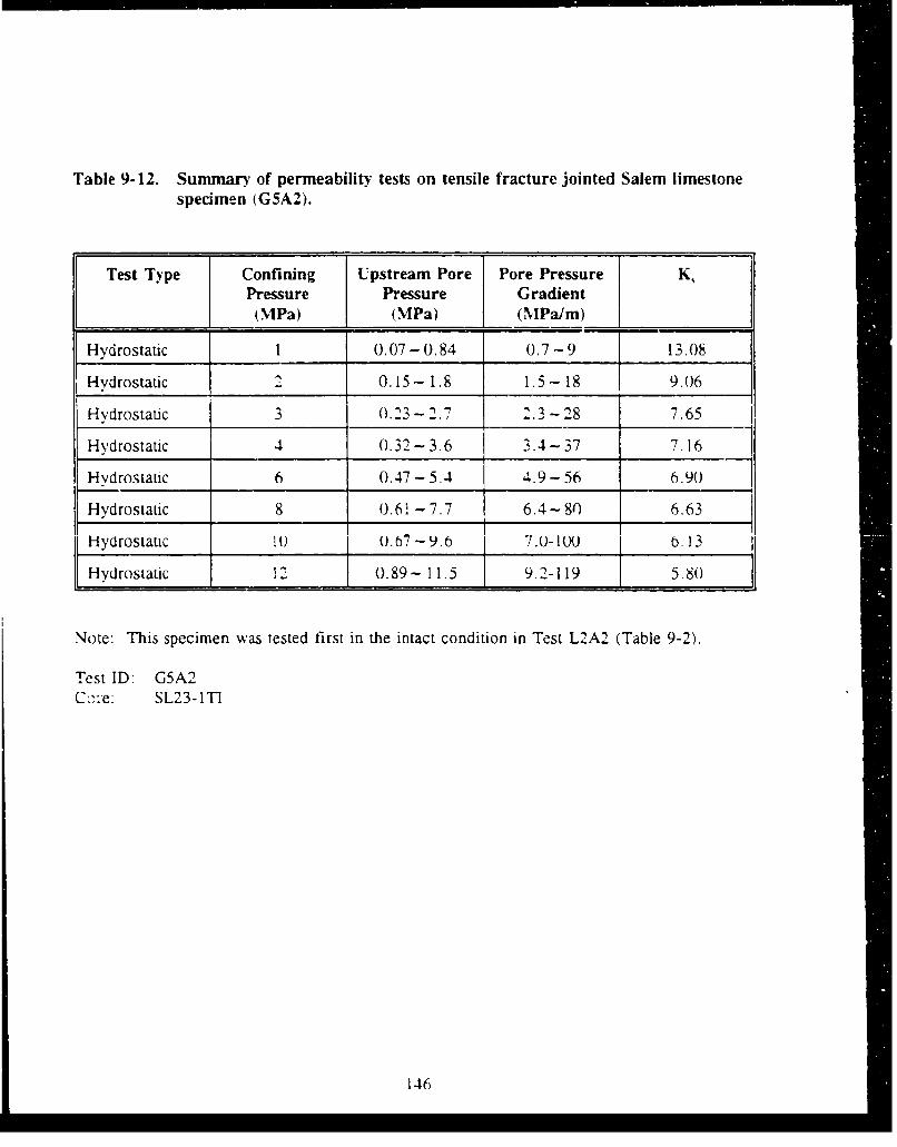
Table 9-12. Summary of permeability tests on tensile fracture jointed Salem limestonespecimen (GSA2).

Test Type Confining Upstream Pore Pore Pressure K,

Pressure Pressure Gradient(MPa) (MPa) (MPa/m)

Hydrostatic 1 0.07 -0.84 0.7-9 13.08

Hydrostatic 2 0.15- 1.8 1.5- 18 9.06

Hydrostatic 3 0.23- 2.7 2.3 - 28 7.65

Hydrostatic 4 0.32-3.6 3.4- 37 7.16

Hydrostatic 6 0.47-5.4 4.9-56 6.90

Hydrostatic 8 0.61 -7.7 6.4-80 6.63L ydrostatic 1 (J.b7-9.b 7.0-1lX b. 13

Hydrostatic 12 0.89- 11.5 9.2-119 5.80

Note: This specimen was tested first in the intact condition in Test L2A2 (Table 9-2).

Test ID: G5A2C ý-.-e: SL23-1TI

146

Table 9-13. Summary. of permeability tests on tensile fracture jointed Salem limestonespecimen (OAA282).

Test Type Confining Upstream Pore Pore Pressure K,Pressure Pressure Gradient

(MPa) (MPa) (NIPa/m)

Hydrostatic 1 0.07-0.8 0.8-8 15.43

Hydrostatic 2_0.15-1.8 1.5- 17 8.62

Hydrostatic 3 0.21-2.7 2. 1 - 28 6 32

Hydrostatic 4 0.29 - 3.6 3.0-37 5.44

Hydrostatic 6 0.44-5.4 4.6-56 5.03

Hydrostatic 8 0.60-7.2 6.2-74 4.82

Hydrostatic 10 0.73-9.6 7.6-100 4.46

Hydrostatic 12 0.88- 11.5 9.2-120 4.66

Note: This is a repeat of Test G5A2 (Table 9.12).

Test ID: OAA282Core: SL3 3 -1

147

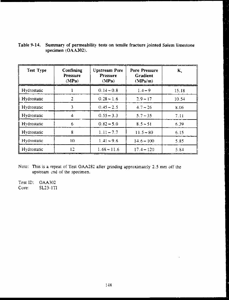
Table 9-14. Summary of permeability tests on tensile fracture jointed Salem limestonespecimen (OAA302).

Test Type Confining Upstream Pore Pore Pressure K,Pressure Pressure Gradient

(MPa) (MPa) (MPa.m)

Hydrostatic 1 0.14-0.8 1.4-9 15.18

Hydrostatic 2 0.28-1.6 2.9- 17 10.54

Hydrostatic 3 0.45- 2.5 4.7 - 26 8.06

Hydrostatic 4 0.55-3.3 5.7-35 7.11

Hydrostatic 6 0.82-5.0 8.5-51 6.39

Hydrostatic 8 1.11 - 7.7 11.5-80 6.15

Hydrostatic 10 1.41-9.6 14.6-100 5.85Hydrostatic ] 12 1.68- 11.6 17.4- 120 5.84

Note: This is a repeat of Test OAA282 after grinding approximately 2.5 mm off theupstream -nd of the specimen.

Test ID: OAA302Core: SL23-1TI

148

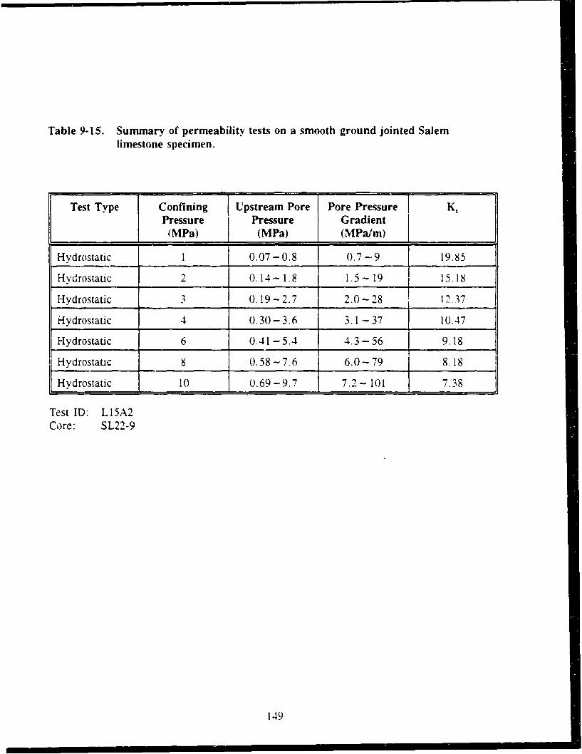
Table 9-15. Summary of permeability tests on a smooth ground jointed Salemlimestone specimen.

Test Type Confining Upstream Pore Pore Pressure K,Pressure Pressure Gradient

(MPa) (MPa) (MPa/m)

Hydrostatic 1 0.07-0.8 0.7-9 19.85

Hydrostatic 2 0.14-1.8 1.5- 19 15.18

Hydrostatic 3 0.19-2.7 2.0-28 12.37

Hydrostatic 4 0.30-3.6 3.1 - 37 10.47

Hydrostatic 6 0.41-5.4 4.3-56 9.18

Hydrostauc 8 0.58-7.6 6.0- 79 8.18

Hydrostatic 10 0.69-9.7 7.2- 101 7.38

Test ID: L15A2Core: SL22-9

149

Table 9-16. Summary of permeability tests on a synthetic jointed Salem limestonespecimen with synthetic fracture.

Test Type Confining Upstream Pore Pore Pressure K,Pressure Pressure Gradient(MPa) (MPa) (MPa/m)

Hydrostatic 1 0.07-0.7 0.7-7 883

Hydrostatic 2 0.15-1.1 1.6 - 12 546

Hydrostatic 3 0.21-1.5 2.2- 16 427

Hydrostatic 4 0.29- 1.8 3.0- 19 343

Hydrostatic 6 0.35-2.6 3.6-27 228

Hydrostatic 8 0.35-3.6 3.6-37 179

Hydrostatic 10 0.34-4.5 3.5-46 140

Hydrostatic 12 0.41 - 5.2 4.3-54 112

Test ID: L20A2Core: SL22-7

150

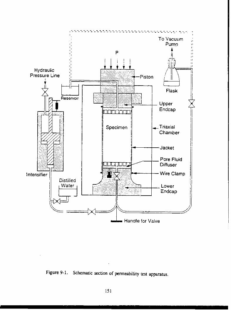
To VacuumPumo ,

P 4I I "I

I I II i n

Hydraulic "Pressure Line \. . -Pi./ I

\\ '" \"\\\ Flask

Reservoir L: • Upper

__ -"Endcap

Specimen .. _TriaxialChamber

"•"'•'••!i'•" -- Jacket ,

'' -, I !,, Pore Fluid

Intensifier Wire Clamp

Distilled/Water / I ___ Lower

I / '2 "1 .•; Endcap

on" - Handle for Valve

Figure 9-1. Schematic section of permeability test apparatus.

151

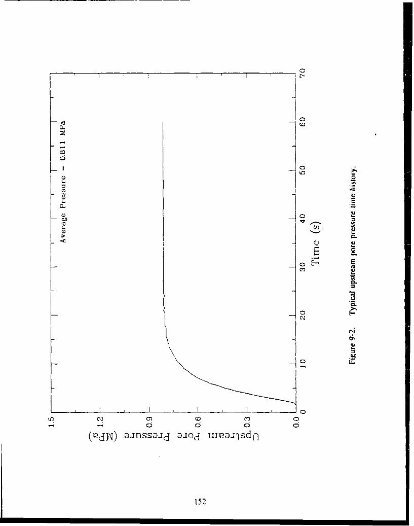
0_ II 0

152

L. E

L 0 F--

L J L I

C\ 0

(•dt•) G-flSS~c Jd m urax•sdf

152

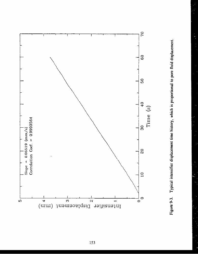
o d-

, U,

1 0a

00

_mn co CN

L II1 I -

(u-iui) ju~qu-iaopds!G xlai1!sualul153

153

V..

000>

C I-

- Cu

}\ '" 1 r,.,

~'/~~dY 4) 0POIA pjnM juaxmddv/-4uaipeJD aiflssaid

154

154

ct,

- -

0 v

K #1

I- -

.2

r I005

I QI-iKi

iiii_______i___ii____________-___-__-_-___________-:I

F --

K 7I

I-

I D

0

0- 0o

•,r

V ,_ I Q•'¢

F "~0 0 0."

115

k VL

03

.. "-, -IU

c~c,4,"

o 156

I '-

LL

il

0 -0o

2 -7

0 1

-.

2

! -

u• C•• •0c''

. --

"C" ••• X \ -I•

C2r

0 157

I • P.V //LJ/ sV3

'..-

u

ClC

00

ow-

/ .

I ,

-ii"0

(•a._ ),<!fqouIC lnoq <-I-

158

,,,, '- - , -

i iIi I • • I I

C- a..'. /

-• /

vl vl. , ,

rTOC) v\ / -,C:)w CD

0 m C)

vl i 0 - ,C

I L 1-

x

00 OIU

cF "

u .• _ 0 ) i q j l~ q i 2 @ U - 1 a d a -4n -to s q v ,,

LU

159

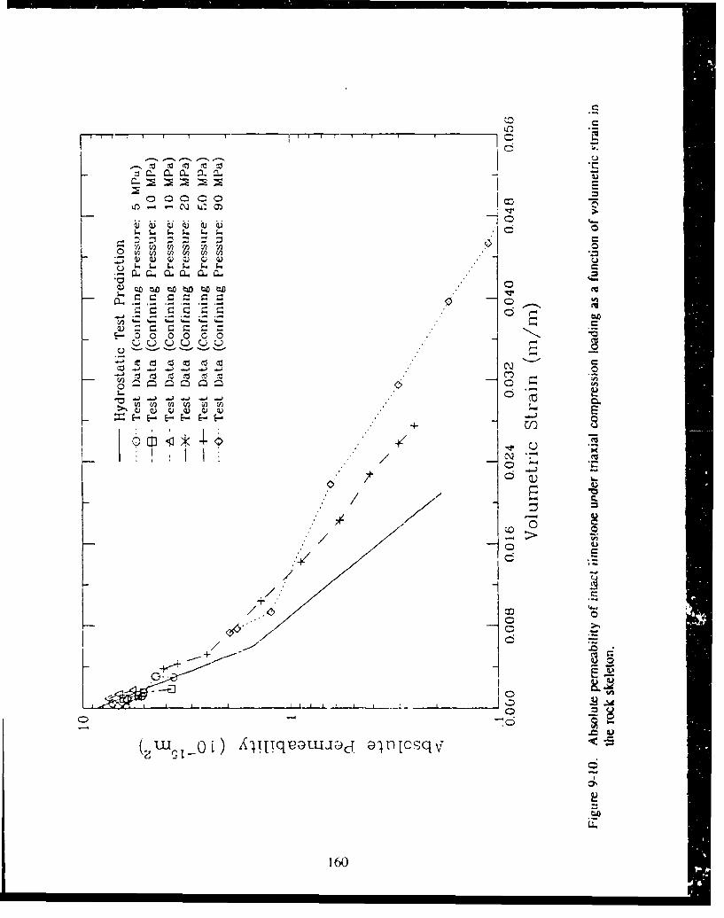
r

LqL1 i i _ -

'-o CQ~ 0

3:11

11) p p p) Q)a. . CL. L C

0 000 0 0

CO -j - -.j -5 C-

co ýz to Co "

'1_0 i

- ) • ) C,.) C) 6O••L2"1 •

160 /

II

o-- o

160 i.

(2QTu, OI) XI!I!•.qeam-•ac a~njosqv "5

V) C"

J N1 -5

00

- iI0

I

-iv

K 0,

0 >1 2

11

c co to 0 0

7 :7

-1 60 61

--1 (I tOI) £.Iqt-Ia a~Iosq

L£t . > '' >' ' -0

A A

7t t

IA KCDF

-a .

oo

(edA) ouZa;-JJaG ssaIS

162

S!

(tL%_O T) X •.iq~W'I• 3 d a-%nIsqv

L22

EE

II

c(

1163

-I

oo

Cl)

o *-

0~0

0 • .. . 4 - C-

-4aua~TT~fl ssaJ1IQ

IIII II II II IIII III II I_163

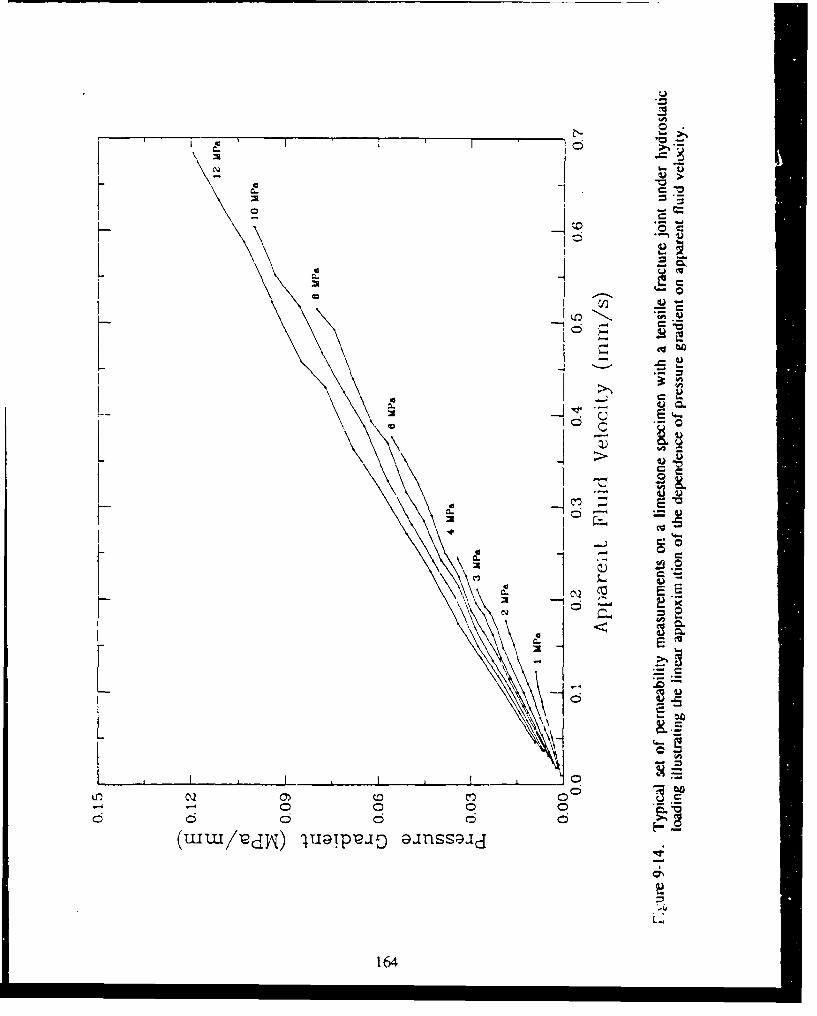
c I=I

cl!i

cc

1 1A0

I0

no.o

2I . .-

Ln Cd

-4 -0 0

SI-

KLL

164

0 00

L 0 I C

C\ <C\'2L

I CD

C)IL I - U ..

0 -4 -II"

(Z-1,_T jjq2@IIJ

_ .

165

L I

' I I It13

C co

- -a ' I

M/

I • -•

cc C

• Io i

166

•_____ , ! , I I 0 "

166

La

I .. -- -II "-' ~

I -

CA

II I "-

h .- "

I - "

"- ,.. I -,

I - -

a.i

o 2l

167

I C,

0 0.I

0 -- -

167

,i il h , I .I I I l II . i , II i I l

I'-

I t-'

0 • "0

C 02--0_

I -i

o '-' .

0U 0_OT) X+2I•quald

!68

I I i i i iI I i1-•l • : i• : -

01) -1c

.5.

i ":1.

'~ - -U

C 0

-. I

I ,-- L4d CLEc

L 0 01i I

II I 1

L

0 1- ' *' .

0 C- 0-

KC2 -•_

u II

169

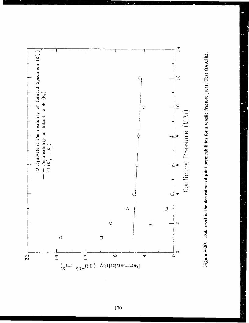
-~ I I

I v.•I 4:

I --

"

I - > -.--

II ._

-- 0• .

.l I I I-

I I I -. . ,

(z _0I)s-½, qImad•

170

F •- I

I •I UI _+

I __

I C, 0 I -.

I .IQ 1.21._...

o nI .- 4.

I / °

----Si Z0 [] "- ..z

00 I -C

o C.o C\ 0 o

171

CQu

-CC -

fi|'-1 1l |i

U

ii

i

N I-0

0 E

CO

Q)L40F

-

L

Cuo

0x,0 X cS

X0 -C

X-4 0 0 C\

0 0 3ci

×D

--

D

--

4

(Oui 1 -_OT) r%

17,2

78

VU

Scc-

0 0 0

I -1-4C C)

(•u-iu) uo!qeuijao

173

CD _L

0_ Co

0

CC0

-- 0o o_

oo -

00

- 00 - -.5

N 0

C)U

000

v174

f0

tw

C. C. Cd

C /2 co

E c

C.z,

b4LoC20 Dc 0C

0t C., 00

L#2

175

vq

0 0-

C/)

V W

0

to 1Q o II

176

i ! I I I I I

T I T

2V{oL

L-4

-I i

So -4

.- - D0

.. " .)

C\ 0 m~~4-

Lo V

C\~203

0

0o

o o 0"-

(m, 91o00 ry

177

to,0.

oI--00

CC

.. 52J

> LV

Ch

CC

00

I I I, J 0 0•':

0 0 CQ C) 0•-00 CD 0 0 C

0 0 0 0 0 5

(nU-Ir/'Pdy{) juipi2.piJf anssa9Jd

178

C\2

U)\

0 [] .0

E,

179

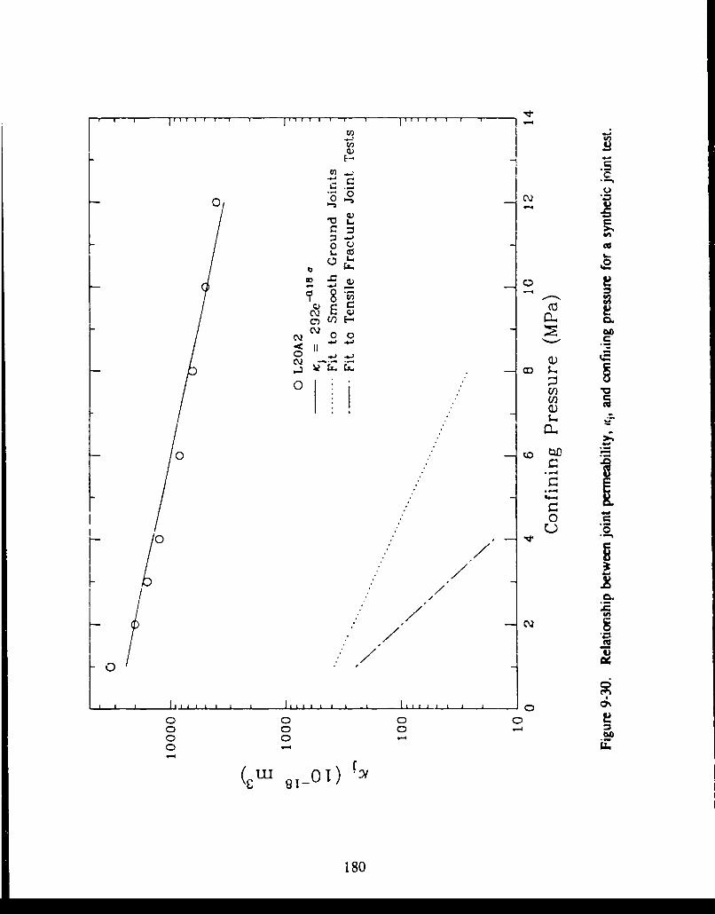
lii"'- ... . . . "'" 1 .. . . ] . . . .

€,\2

Ld

00

° l i......°, 0

.' a'

-' -

0 Q)0) ( 0- m

C\2

0 0/00

... / .• /

-/ C\

18

0 0 0) 0

0 ,-

180

SECTION 10

NUMERICAL SIMULATION OF ROCK JOINT RESPONSE

This section describes the development of a constitutive model for rock joints that can

be implemented in a finite element program tor explicit simulation of joints in a rock mass. The

model treats the joint as a thin porous continuum with finite thickness so that in forming material

constitutive relationships, stresses and strains are used instead of forces and displacements. The

stress-strain relauonships w.ere denved based on elastoplasuc theory, and strain softening in the

brittle and brittle-ductile transition regions are expressed in terms of plastic work. The following

subsections present the theoretical deri',ation of the model, procedures for parameter evaluation,

and a verification problem.

10.1 THEORETICAL DERIVATION OF ELASTOPLASTIC RESPONSE OF JOINTS.

ti ,,j ,, ,,um uo that i e joint has lnlte thickness. Thus the

constitutive relationship is formulated in terms of stress and strain. The stress space is assumed

to be composed of two regions as shown schematically in Figure 10-1. Region I reprcsents the

brittle and brittle-ductile transition zones where continued shearing causes the material to reach

a shear strength limit and then decrease to the residual strength. Region II represents ductile

zone where the stress-strain response of the joint is the same as that of the intact material. In

Region II, the joint shear responses are assumed to be elastic below the strength envelope and

elastoplastic along the strength envelope. In Region I, the joint shear responses are assumed to

be elastic up to the peak strength and elastoplastic with strain softening when the shear strain

is increased beyond the point at which the peak strength is reached. Strain softening in !.i's

region is related to the accumulated plastic work. In the following, incremental stress-strain

relations for softening are derived based on the theory of plasticity.

10.1.1 Notations.

This subsection lists the notation used in the derivation. In keeping with tho usual

geotechnical convention, positive signs indicate compression.

181

{df ) : total strain increment vector

[d•,) elastic stLi.1in increment vector

(d(} plastic strain increment vector

df n normal (axial) strain incremcnt

SE,,, •elastic normal (axial) strain increment

dE,,r •plastic normal (axial) strain increment

d'" shear (tangential) strain increment

dy -• elastic shear (tangential) strain increment

dy • plastic shear (tangential) strain increment

(do'} (effective) stress increment ve.tor

do,, • (effective) normal stress increment

dr shear (tangential) stress increment

P. atmospheric pressure

[DC • elastic stress-strain matrix

rrLep stress-stari ruaW

E Young's modulus

G" " shear modulus

WP -plastic workWp.,=o 5 plastic work at s=0.5

ýr "normalized plastic work

s softening variable

T apparent tensile stiength

17, •yield constant

m yield copstant

0, "residual friction angle

F yield function

G potential function

a softening constant

b softening constant

c plastic potentia' constant

d plastic potential constant

182

10.1.2 Total Strain Increment.

The total strain is comprised of the elastic and plastic components of strain as given by:

{4e} We(i) , {dec} (10.1)

or

10.1.3 Elastic Stress-Strain Relationship.

The incremental elastic constitutive law can be expressed in the following matrix form:

{do§ = [D'] {dE) (10.2)

or

LO G0C] rd2,

The elastic modulus, El, is assumed to be expressed as a function of effective normal sti -ss:

E = E (o,') (10.3)

and the shear modulus is assumed to be constant:

G' = constant (10.4)

183

10.1.4 Yield Equation.

The proposed joint model does not allow hardening. Thus the yield surface coincides

with the failure surface. The joint model, however, allows strain softening which is r,-lated to

the plastic work.

F (oU, e) (o, W, (F.)) : 0 (10.5)

The explicit form of yield equation is given by:

F(o,, -, iP) = (1-s) X,. + s- e = 0 (10.6)aP

where:

1 *tXr - (10.7)tan, Pa

a (10.8)

s = (10.9)

Wp (10. 10)P W p.,s-.

dWP f {oI}T {dp}= = l } {dcP} (10.11)

or

dWf o "d, + t "dyP

184

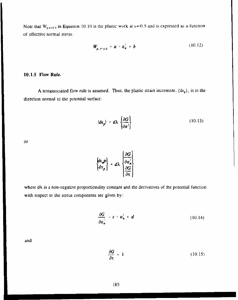
Note that Wp.,.o . in Equation 10. 10 is the plastic work at s=0.5 and is expressed as a-function

of effective normal stress.

W = a • a' + b (10.12)

10.1.5 Flow Rule.

A nonassociated flow rule is assumed. Thus, the plastic strain increment, {dfp}, is in the

direction normal to the potential surface:

{dep} =d, (10.13)

or

[8G1

IdyP j 1)where dA is a non-negative proportionality constant and the derivatives of the potential function

with respect to the stress components are given by:

2 - con +d (10.14)

and

- 1 (10.15)

185

10.1.6 Normal to the Yield Function.

The derivatives of the yield function with respect to the stress components are given by:

faF~JaF c = yno4 (10.16)

where:

aF S (X, X o 693 a t- (10.17)ao'. (aol + b) Pa

and

8F - (1-s) s ?I,& P, ta p0, (2 (10.18)

10.1.7 Consistency Equation.

During yielding, the consistency equation forces the stresses to move along the yield

surface.

dE FIT {do'} + OF+ dW = 0 (10.19)laF-o'jl aw

where:

dW -W {dCP) = {o§"T {dEp} (10.20)

186

Substitution of Equation 10.13 into Equation 10.20 yields:

dWP = dX .{o1IT c'r.} (10.21)

And the partial derivative of yield function with respect to the plastic work is given by:

F = 0.693a WP aon + b

10.1.8 Formulation of Elastoplastic Stress-Strain Matrix.

Equation 10.21 is substituted into Equation 10.19. to obtain:

ida I + =-F T0 (10.23)Lao'i aw,taJ

The elastic strain vector in Equation 10.2 is rewritten in terms of the plastic strain vector using

Equation 10.1, to obtain:

{do} = [D9 (idel - {fdp}) (10.24)

The plastic strain vector in Equation 10.24 can be expressed in terms of the derivatives of

potential function with the aid of Equation 10. 13.

(do') = [Dr] del - [D9 d){_} (A0.25)

Now substituting Equation 10.25 into Equation 10.23 and solving for dA, to obtain:

187

TaF [D9 (de)

A ac (10.26)T[D9 8G _ aF iqT aG.

By backsubstituting this dX into Equation 10.25, the effective stress increment is directly related

to the total strain increment as follows:

{da"} = [DeP] {de} (10.27)

where the incremental elastoplastic constitutive matrix is expressed as:

[D` [DI

[D tP] z [D T- a-- (10.28)

1J)9 I n[Dl -I W o J8G

10.2 EVALUATION OF MODEL PARAMETERS FOR TENSILE FRACTURE JOINTS

OF SALEM LIMESTONE.

Section 10.3 presents an example of the joint model used to predict the stresses and strain

softening for specified input strains. The determination of material parameters used in that

verification problem are described in this secdon. Since the development of the model was done

in parallel with the laboratory testing, the example is based on test data from a previous joint

testing effort (Chitty and Blouin, 1992).

188

10.2.1 Elastic Constants.

Based on the unload and reload slopes of unconfined compression tests of tensile fracture

joints, the following elastic modulus (E_,) and shear modulus (G') for a fully closed joint were

obtained.

F_ = 31,000 MPa

G" = 12,500 MPa

10.2.2 Joint Compressibility.

The model treats the joint as a thin continuum with finite thickness so that determination

of the joint thickness is necessary to relate the measured joint displacements to joint strains.

Joint thickness, t consists of the average thickness of roughness, t, and the gap between top and

bottom surfaces, t8 . That is,

t = t, + ts (10.29)

The roughness, t4, was estimated as 0.66 mm from the joint profile shown in Figure 10-2. The

gap, t., was estimated from the normal compressibility test (A3CO). The value for t, of 0.074

mm was obtained at the lock-up point of the joint normal displacement. Thus, from the

Equation 10.29, the esti,.I.•ted joint thickness is

t = 0.66 + 0.074 = 0.73 mm

Figure 10-3 presents the results of a normal compressibility test on a tensile fracture joint

in Salem limestone. In this test, a V-shaped groove approximately 3 mm deep was cut around

the circumference of the limestone specimen at mid-height. Two sets of mounting fixtures were

attached to the sides of the specimen with epoxy adhesive and LVDTs were attached to measure

axial deformation of a portion of the specimen including the groove at two diametrically opposed

locations. The specimen was loaded axially in unconfined compression and the output of the

axial deformation gages was recorded and averaged. The solid line labeled "Pre-Fracture" in

Figure 10-3a represents that record. Without disturbing the LVDT mounting fixtures, the

specimen was placed ir "ecial grips and loaded in tension until it broke along the groove,

189

creating a tensile fracture joint. It was then re-loaded in unconfined compression. The data

recorded in that test are shown as the dashed line in Figure l0-3a labeled "Post-Fracture". The

difference betwe,..n those two displacements, which is shown in Figure l0-3b. represents the

normal displacement of the joint, assuming that the joint has no thickness when it is completely

closed. Hovwever the model formulation, presented here is based on the assumption that the joint

has a finite thickness. The following analysis was performed to convert the data to a form that

will support this analysis.

It is necessary to estimate gage length (h) to interpret the joint normal compressibility

data shown in Figure 10-3 in terms of axial stress and strain. Figure l0-3a shows the axial

stress vs. axial displacement plot for intact sample (A3AO). The axial displacement U, at

a = 30 MPa is 0.016 mm. Since the Young's modulus of intact Salem limestone is

q= 31,000 MPa, the axial strain of the intact sample at a.' = 30 MPa can be computed as:

!o,, 30 _

C -30 - 0.00097E, 31,000

Thus the gage length can be estimated from the measured displacement and the computed strain

as:

h = U, . 0.016 - 16.5mmel 0.00097

To support the analysis assuming finite joint thickness, the joint stress-strain curve was

computed from specimen normal displacement, U•, represented by the Post-Fracture curve in

Figure l0-3a, by subtracting the elastic deformation of the material in the gage length less the

joint thickness, t, as follows:

19U - (h at E

190

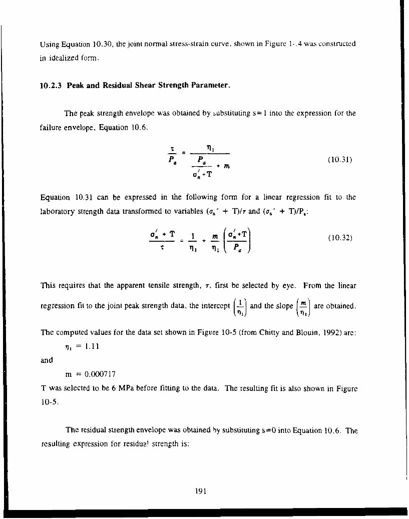
Using Equation 10.30, the joint normal stress-strain curve, shown in Figure 1-.4 was constructed

in idealized fom.

10.2.3 Peak and Residual Shear Strength Parameter.

The peak strength envelope was obtained by ,ubstituting s= 1 into the expression for the

failure envelope, Equation 10.6.

P, P i_(10.31)

On+T

Equation 10.31 can be expressed in the following form for a linear regression fit to the

laboratory strength data transformed to variables (a,, + T)/r and (a,, + T)/P,:

/+Ton+T 1 _ m (10.32)

This requires that the apparent tensile strength, T, first be selected by eye. From the linear

regression fit to the joint peak strength data, the intercept and the slope ( J are obtained.

The computed values for the data set shown in Figure 10-5 (from Chitty and Blouin, 1992) are:

= 1.11

and

m = 0.000717

T was selected to be 6 MPa before fitting to the data. The resulting fit is also shown in Figure

10-5.

The residual strength envelope was obtained by substituting s=0 into Equation 10.6. The

resulting expression for residual strength is:

191

tan (10.33)-=tart *-."

The residual friction angle, 0, = 40', was obtained by a straight line fit to the sawcut joint

strength as shown in Figure 10-5.

10.2.4 Strain Softening Parameter.

The joint model assumes that the strain softening is related to the normalized plastic

work, Ep, which is related to the softening variable, s, by Equation 10.9. Thus. when ýp = 0,

s= 1 and yield equation coincides with peak strength envelope. When ýp = 1, s = 0.5 and

yield equation is half way between the peak and residual strength envelopes. When tp

approaches infinity, s= 1 and the yield equation coincides with the residual strength envelope.

It should be noted that tp in Equation 10. 10 is the current plastic work, W., normalized

by the plastic work at s=0.5 (Wp.,,.(o). As shown in Figure 10-1, the triaxial compression

stress path for a given confining pressure, a.', crosses the yield equation (s=0.5) at the stress

point (a. ', r,). From a plot of joint shear stress, r as a functioti of plastic work WP, for each

confining pressure, Wp.,=_ 5 at r=rm is found, as shown in Figure 10-6. For each confining

pressure, u.,' and Wp. -0 are listed in Table 10-1. The softening parameters, a and b, in

Equation 10.12 can be found by a least squares fit to the data as shown in Figure 10-7. The

resulting values are.

a = 0.474

b = 1.7

10.2.5 Plastic Potential Parameters.

The flow rule specifies the direction of the plastic straini increment. This model uses a

nonassociative flow rule so that the plastic strain increment vector is normal to a potential

surface which is different from the yield surface.

192

The plastic potential parameters, c and d in Equation 10. 14, can be related to the slope

of the normal to the shear strain by combining Equations 10.13, 10.14, and 10. 15.

aoa c' - • I + d (10.34)&G dyp

Figure 10-8 shows the measured joint normal displacement plotted as a function of joint

tangential displacement at confining pressures of 1, 5, 10, 15, and 20 MPa. The slope of these

curves represents very closely the ratio of the normal to shear plastic strain increment in

Equation 10.34 since the elastic strains in this softening region are very small compared to the

plastic strains. Figure 10-9 shows the values of these slopes plotted as a function of the effective

normal stresses. These effective normal stresses are not the confining pressures but the stresses

at the average of peak and residual strength envelopes. A least squares fit to the data gives the

following plastic potential parameters:

c = 0.00783

d= -0.236.

10.3 VERIFICATION PROBLEM.

This section presents two verification problems for the material model using the

parameter values for tensile fracture joints in Salem limestone that were determined in Section

10.2. The incremental constitutive relations were formulated in the form of stiffness matrix.

Thus, for a known strain increment, the constitutive matrix computes the corresponding stress

increment. For verification, the model will be used to simulate laboratory triaxial compression

tests. Two triaxial tests at confining pressures of 5 and 15 MPa were selected. The ratio of

input normal strain to shear strain is estimated as -0. 133 for 5 MPa confining test and 0.029 for

15 MPa confining test based on the measured displacement slopes shown in Figure 10-8. Both

predictions begin at stress points on the peak strength envelope and continue until they approach

to the residual strength envelope.

193

Figure 10-10 shows predicted and measured stress paths during the strain softening

portion of triaxial compression test. Though the predicted stresses do not decrease as a single

straight line as in the triaxial compression test, the trend of predicted stress paths geiierally

follows those measured in the laboratory. Figure 10-11 shows predicted and measured strain

softening plotted as a function of plastic work. There is good agreement between the predicted

and measured strain softening.

10.4 CONCLUSIONS RELATED TO JOINT SIMULATION.

A joint material model was developed based on the results of laboratory tests conducted

on tensile fracture joints of Salem limestone. The proposed joint model is a first step in the

development of more complicated models for in situ rock joints. In addition to multi-linear

segments for the normal compressibility, the joint model has nine parameters describing elastic

and elastoplastic responses with strain softening. These material parameters can be

systematically cxtracted from laboratory test results as described in Section, 10.2. The joint

model can easily be adapted to a continuum based numerical simulation program to represent

the discontinuities between intact rock blocks.

194

Table 10-1. Plastic work at s=0.5 tabulated as a function of normal stress.

Confining Pressure Average Normal WP. =,0. in in Straino'., (MPa) Stress Displacement (NIPa)

g"' (MPa) (MPa-mm)

1 7.95 3.5 4.8

5 16.95 6.5 8.9

10 25.14 11.5 15.8

15 34.(X) 13.5 18.5

"20 42.60 15.0 20.5

Note that joint thickness t=0.73 mm is used to compute strains from displacements.

195

Pa

Pt --- - - - -

at s=0.5, t -m - - --- 1 ,

Region I Region II

nm anb Pa

Pa Pa

Triaxial Compression Stress Path

ln- lCn +tanO 1-Pa Pa Pa

Residual Strength Envelope (s=O)0n1 1t

Xr Pa tanOr Pa

Yield Equation During Strain Softening

n = (1-s) •r + S Xp

Pa Where s = e p

Peak Strength Enveiope (s=l) T

'n Paxp n = = " (+xP Pa Pa rl n T

a aa

Figure 10-1. Illustration of the yield and strength envelopes for the joint model.

196

_LL4

-2

-40 | 10 20 30 40 50

-- fý ImmA Z= 5mm

Figure 10-2. Measured joint roughness profile that was used to derive the joint thickness.

197

30

. . . . . .. . ... . . . . . . . . .. . . . . . .. . . . . . .

• ----. . .Pre-Fracture

nL ,- Post-Fracture

20 .. ... . ........ ........ .......... r ....... ......... . . ... ...... .. ........ ........

.. ..... .. ....... ......... ....... / ,' ........ . ........ . .... .. ......... ......... ........

10 .

10. ................ * .........................

. .... =........ . . ....... ......... ........ ..- ........ -......... ........

0 0.4 o 0.12 0.16 02Axial Defomiation (ram)

Figure 10-3a. Axial deformation measurements from an unconfined normal compressibilitytes on a tensile fracture joint.

30

2 . . ....... . ........ .. .... ... .. ... .. .. ....... .. ...... . ..... . ........ , ........ , . . . .

r75~~I ..........

S2 0 . . . . . . * . . . . . . . . . . . . . . . . . . . . . . ,. . . . . . . . . . . . . .. . . . . . . . . .. . . . . . . . . .. . . . . . . . . .. . . . . . . . .

(D)

* ..

0 •0 0.04 0.08 012 0.16 0.2

Joint Normal Deformation (mm)

Figure 10-3b. Joint compressibility curme deriveo from the data shown in Figure s l-3a.

198

C>B

co

c,0 Lu,

c6

-~0E

(u, X A .D

C~C)

06ri

0 0oC*

(ed"l '4 D) SS8J1(, I9!XV eAIP193o4 iuior

199

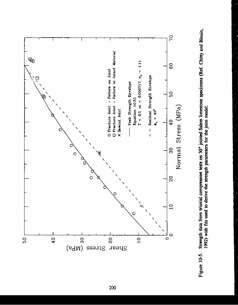
C)C

oo

to

0 v

00

Z Is

10 140

0J 0 x

N 0.. If

C\

D 0 00 0

U-)~g .C c -4 -

(PdWI) ss@aIS .uaqS •

200

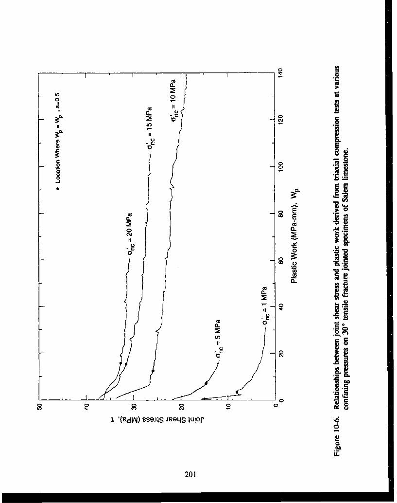
i " I' '~ ~~ I ' I I '"

II In "Z

C.L

- .-

~:cL II

C.'ed ) *i.l eesluo

SE

EE

2-2

CII I

Cu L

0L 0

CVl

2011

0 I~0 I

b eQC

'ob

S0

S00

II~

v0

tD Q20200

00

CQ -l - , - L

('edi) 9o =0

202

'Ic

Si

Q)02

/C

IQ U

'a. a. CL (LC

V -V

0o

C6

,i i '!

L 00

203

0 1l

+ .o

C:

CQCu

olo0

uo,--soidtuo- c.•K

+) 0 oII

(p)/ p)204

II -2ob

I I

M 0

t~ cc

4 -1)

U))

IL-

'(- oO (U.

--

"', U,

\\O

0D0

"U, 0

0 V

", 2

(Bdl/Y) SSe94S Jee(qS r,

205

CD

E

M~ .0', ' 5

W

(D

o

*--

2O0

IE Ee0-

0

*.13

(EVY 0sjcjeq o

I-T

206

SECTION 11

ASTM/ISR INTERLABORATORY TEST PROGRAM

This section presents the results of laboratory rock property tests performed by ARA as

part of the Interlaboratory Testing Program for Rock Properties, which is being conducted by

the Institute for Standards Research. a subsidiary of the American Society for Testing and

Materials. The laboratory work was performed by ARA's Materials Testing Laboratory located

in South Royalton, Vermont during August and September 1991, and during May and June

1993.

The test program was conducted in two parts. Under Phase 1, ARA prepared and tested

specimens of four different types of rock:

Barre granite 2.645 Mg/m3

Berea sandstone 2.150 Mg/m'

Salem limestone 2.265 Mg/m'

Tennessee marble 2.690 Mg/mr

After an extensive series dimensional and tolerance measurements, all four rock types were

tested to determine ultrasonic wavespeeds in compression and shear; elastic constants and

strength in unconfined compression; and splitting tensile strength. Under Phase 2 of the

program, the same types of rock, except Salem limestone, were tested in triaxial compression

to determine elastic constants and strength. The Phase 2 tests were performed on specimens that

were supplied in finished form by the study's organizers.

11.1 SPECIMEN PREPARATION AND MEASUREMENT.

For the Phase 1 tests, the rock materials were supplied to ARA in the form of cores with

rough ends. The specimens for the Phase 2 tests were supplied in finished form with ground

207

ends. In both phases of the program. dimensional tolerance checks were made by the ARA

laboratory prior to testing.

11.1.1 Phase 1 Specimen Preparation.

The sample material of all four rock types arrived at the ARA laboratory in the form of

cores approximately 55 mm in diameter and 225 mm in length. Of each rock type four

specimens were prepared with length to diameter ratio (L/D) in the range of 2.0 to 2.5 for

unconfined compression testing, and four were prepared with L/D between 0.5 and 1.0 for

splitting tensile tests.

The cores were cut to the required lengths and the ends were ground using a 170 grit

diamond wheel on a precision surface grinder. The specimens for the unconfined compression

tests were prepared with their ends parallel within 0.0005 in. over the specimen diameter. For

each specimen that was to tested in unconfined compression a complete dimensional tolerance

check 'vas performed in accordance with ASTM D 4543, and all specimens were in conformance

with the specification prior to testing. In addition since the tests were not conducted with a

spherical bearing head in the load path, the protocols for the interlaboratory test program

required that the ends be parallel to each other witrun 0.00U* incf (0.013 mm) over the (nominal

54-mm) specimen diameter. Since no method was specified, determination of parallelism of the

ends was based on the measurements were used to evaluate end flatness and perpendicularity,

as specified by ASTM D 4543, Paragraph 5.2. Special care was taken with these measurements

to ensure that the specimen was not moved in the V-block while both ends were measured.

11.1.2 Phase 2 Specimen Preparation.

For Phase 2 of the interlaboratory test program, the program organizers supplied the

specimens to ARA in finished form with ground ends. These specimens were measured in the

ARA laboratory to insure that they met the dimension tolerances specified by ASTM D 4543.

208

11.2 ULIRASONIC WAVESPEED MEASUREMENTS.

Ultrasonic compression and shear wavespeeds were measured in accordance with ASTM

D 2845 on the Phase I test specimens prior to destructive testing. These measurements were

made using two piezoelectric transducers, one to send and one to receive, and a 20 MHz digital

storage oscilloscope to measure the transit time. The P-wavespeed measurements were made

on the same specimens that were later used for the unconfined compression tests, having length

to diameter ratio approximately equal to two (L/D = 2). Since the shear waves were highly

attenuated over the 100-mm length of the unconfined compression test specimens, the shear

wavespeeds were measured on the splitting tensile test specimens which had L/D < 1.

The results of the waves.need determinations are summari7ed for each rock type in Tables

11- I through 11-4. Each table presents the mean of the five wavespeed measurements for each

specimen of a given rock type, and the mean and standard deviation of the individual specimen

means.

11.3 UNCONFINED COMPRESSION TESTS.

Elastic constants arJ unconfined strengths were determined from unconfined compression

tests conducted in accordance with ASTM D 3148 and D 2938. The tests were performed in

a press designed by ARA that is typically used for triaxial compression testing of rocks at

confining pressures up to 400 MPa and axial loads up to 3.5 MN. It is a four-column frame

with movable crosshead. In the unstressed condition, the upper and lower loading surfaces are

parallel within 0.005 mm (0.0002 inches) over their entire 3-inch diameter. The machine is not

equipped with a spherical head. This is the same machine used to conduct the Pilot Tests.

Aluminum rings of slightly larger diameter than the test specimen were attached near the

top and bottom of the specimen by means of three set screws with conical pointed tips spaced

1200 apart. The two axial LVDTs were attached to the rings at diametrically opposite locations.

The LVDT body was attached to the top ring and a rod connected to the LVDT core was affixed

209

to the bottom ring. This resulted in a gage length of appioximately 0.40 inches less than the

specimen length. A third floating ring was used to hold a single radial LVDT. The radial

LVDT was clamped to the ring with the core rod spring loaded to maintain contact with the

specimen. A screw on the opposite side of the ring served as a reference point for the radial

deformation measurement. A strain gage bridge load cell in the load path provided a

measurement of the applied load. The load and deformation measurements were digitized at 1-

second intervals and recorded by a microcomputer based digital data acquisition system.

Tables 11-5 through 11-8 present the unconfined compressive strength and values of

elastic modulus and Poisson's ratio determined at 25%, 50%, and 75% of the unconfined

strength. The modulus and Poisson's ratio values were determined by a least squares fit to the

appropriate data set over a range of ±5% of the unconfined strength around the nominal value.

Plots of the measured axial and radial strain against axial stress and of axial strain against radial

strain are presented in Appendix F for each test specimen.

11.4 SPLI'ITING TENSILE STRENGTH TESTS.

Splitting tensile strengths of the four rock types were determined in accordance with

ASTM D3967, as modified by the protocols. The tests were performed in the same load frame

as the unconfined compression tests. As instructed by the test protocol, bearing strips were from

the cardboard approximately 0.7 mm thick. The specimens loaded on the orientation line that

was marked on the specimen material provided by the committee. The times for loading the

various specimens ranged between 3 and 6 minutes. In all cases, failures occurred along the

plane of loading. Tables 11-9 through 11-12 present the test results including specimen

dimensions and summary statistics.

11.5 TRIAXIAL COMPRESSION TESTS.

Triaxial compression tests were performed under Phase 2 of the interlaboratory test

program on specimens of three rock types, Barre granite, Berea sandstone, and Tennessee

210

marble. Four specimens each of three different rock types were tested at confining pressures

of 10, 25, and 40 MPa. for a total of 36 tests. The tests were performed in a triaxial apparatus

which was designed by ARA, and has ciosed-loop servo control of both the confining pressure

and axial loading piston. It is a four-column frame with movable crosshead. In the unstressed

condition, the upper and lower loading surfaces are parallel within 0.005 mm (0.0002 inches)

over their entire 3-inch diameter. The machine is not equipped with a spherical head.

All specimens were oven dried prior to testing. The tests were performed with the test

specimens at room temperature (approx. 20'C). In preparation for testing, each specimen was

placed between hardened steel endcaps without lubricating materials. To separate the specimen

from the confining fluid, a jacket of heat-shrinkable polyolefin tubing was placed over the

specimen and shrunk to a tight fit. The ends of the jacket were sealed to the steel endcaps with

epoxy adhesive and held in place with wire clamps.

Measurements of specimen deformatiuns were made with two axial LVDTs and two

radial LVDTs placed as indicate in Figure 4-1. Two radial deformý..ion measurements were

made at locations oriented 900 to each other. The two radial gages were as close as practical

to mid-height of the specimen, one approximately 10 mm below and the other approximately 10

mm above. In both the axial and radial directions, the two deformation gage outputs were

averaged and scaled to obtain the reported radial deformation strains. The axial load was

measured with a load cell placed directly on top of the top cap, inside the pressure vessel. This

location avoids any errors due to seal friction. The load cell consists of a solid steel cylinder

with eight strain gages wired into a full bridge. The load cell was designed and built by ARA.

The load and deformation measurements were digitized at 1-second intervals and recorded by

a microcomputer based digital data acquisition system. The calibrations of all of the instruments

used to measure the pressure, load, and deformation are traceable to NIST.

Tables 11-13 through 11-15 present the values of elastic modulus and Poisson's ratio

determined by least squares fits to the appropriate data sets over the ranges. 25-50% of peak

axial load and 40-60% of peak axial load for Barre granite, Berea sandstone and Tennessee

211

Marble, respectively. Each fit included approximately 50 data points. Appendix F contains a

complete set of response data from the triaxial compression tests, including plots of axial and

radial strain against stress difference and of axial strain against radial strain.

212

Table 11-1. Summary of ultrasonic wavespeed measurements on Barre granite.

Specimen Rock Compression ShearID Type (km/s) (km/s)

BG/91/1-7 Barre Granite 3.54 2.30

BG/91/2-15 Barre Granite 3.52 2.48

BG/91/3-4 Barre Granite 3.53 2.55

BG/91/5-4 Bare Granite 3.53 2.50BG/91/6-8 Barre Granite 3.57 2.48

I-I

Mean 3.54 2.46

Std.Dev. 0.017 0.085

Coef. of Var. 0.49% 3.45%

213

Table 11-2. Summary of ultrasonic wavespeed measurements on Berea sandstone.

Specimen Rock Compression ShearID Type (km/s) (km/s)

BS/91/1-7/1 Berea Sandstone 2.13 1.51

BS/91/2-15 Berea Sandstone 2.20 1.43

BS/91/3-4 Berea Sandstone 2.18 1.51

BS/91/4-1 Berea Sandstone 2.07 1.48

BS/91/4-16 Berea Sandstone 1.99 1.46

Mean 2.11 1.48

Std.Dev. 0.077 0.031

Coef. of Var. 3.62% 2.07%

214

Table 11-3. Summary of ultrasonic wavespeed measurement on Salem limestone.

Specimen Rock Type Compression ShearID (kin/s) (kmls)

SLI91/l-7 Salem Limestone 4.30 2.48

SL.91/2-4 Salem Limestone 4.35 2.36

SU/91/3-3 Salem Limeston'm 4.32 2.35

SL/91/3-20 Salem Limestone 4.34 2.40

SL/91/4-15 Salem Limestone 4.37 2.37

Mean 4.34 2.39

Std.Dev. 0.024 0.047

Coef. of Var. 0.56% 1.97%

215

Table 11-4. Summary of ultrasonic wavespeed measurements on Tennessee marble.

SpwImen Rock Compression Shear

TM/91/1/2-19 Tennessee Marble 5.98 3.48

TM/91/3/2-19B Tennessee Marble 6.40 3.28

TM/91/4/1-2 T&B Tennessee Marble 6.26 3.41

TM/91/4/2-5 T&B Tennessee Marble 6.27 3.29

TM/91/4/2-20 Tennessee Marble 6.36 3.35

Mean 6.25 3.36

Std.Dev. 0.147 0.075

Codf. of Var. 2.35% 2.24%

216

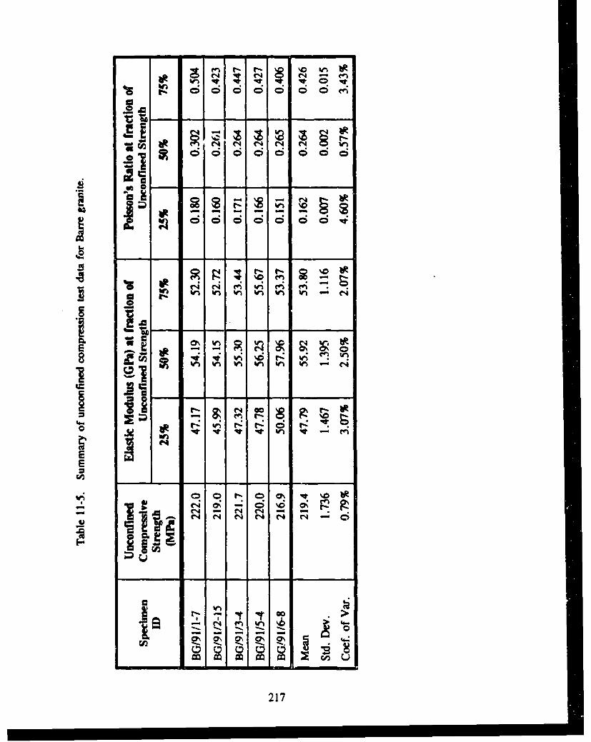
-m -ý -ý %C t

FS~ - maý

t. -: C

C4C "1 1SL

v~ ~ -0lii ___

&~&F'It

21

00

090

C(4

C4 V0 (4 M -

&&&&& &e.4.e4

U, ~ c co - %n q q -

MI1 - ___p

0\Ch ON0%O

21

I -- - -" o'n - '0 r4 0

- - " • ' ' .0

C4 <4 C4 4 * 0

2 • 6•o6• 0'

*

a 4 r4 4 C * C

W! W! '0 '.0 V

; -: • •

1 - -d

00 ~ ~ fl g

~~c c dlim en -4

219

'RD I - I I

t ON 00 00

op *l 4 N ; m

1 00

-~%O0%14 0-0

co P. wl

.2 ; 0ý %

go t-

LEW

22

Table 11-9. Splitting tensile strength data for Barre granite.

Specimen Specimen Dry TensileSpecimen Rock Length Diameter Mass Strength

ID O (in.) (in.) (g) (MPa)

BG/91/l-7 Barr Granite 1.655 2.169 264.4 16.17

BG/91/2-15 Barre Granite 1.595 2.169 255.1 13.77

BG/91/3-4 Barre Granite 1.591 2.169 254.2 14.12

BG/91/5-4 Barre Granite 1.629 2.168 260.1 14.46

BG/91/6-8 Barre Granite 1.594_ 2.172 255.5 14.33

Mean 14.57

Std. Dev. 0.833

Coef. of Var. 5.72%

22-

221 .

Table 11-10. Splitting tensile strength data for Berea sandstone.

Specimen Specimen Dry TensileSpecimen Rock Length Diameter Mass Strength

ID Type (in.) (in.) (g) (MPa)

BS/91/1-7/1 Berea Sandstone 1.648 2.148 207.2 3.94

BS/91/2-15 Berea Sandstone 1.689 2.152 213,7 3.86

BS/91/3-4 Berea Sandstone 1.667 2.157 212.7 4.04

BS/91/4-1 Berea Sandstone 1.649 2.169 211.0 3.61

BS/91/4-16 Berea Sandstone 1.619 2.169 207.9 3.77

Mean 3.84

Std. Dev. 0.147

Coef. of Var. 3.83%

222

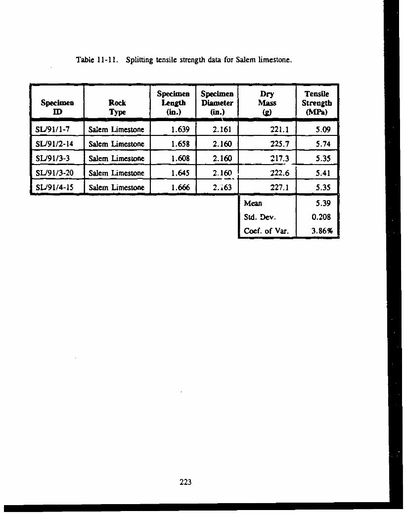
Table 11-11. Splitting tensile strength data for Salem limestone.

Specimen Specimen Dry TensileSpecimen Rock Length Diameter Mass Strength

ID Type (in.) (in.) (g) (MPa)

SIJ91/1-7 Salem Limestone 1.639 2.161 221.1 5.09

SL/91/2-14 Salem Limestone 1.658 2.160 225.7 5.74

SLJ91/3-3 Salem Limestone 1.608 2.160 217.3 5.35

SL/91/3-20 Salem Limestone 1.645 2.160 222.6 5.41

SLI91/4-15 Salem Limestone 1.666 2.1'63 227.1 5.35

Mean 5.39

Std. Dev. 0.208

Coef. of Var. 3.86%

223

Table 11-12. Splitting tensile stre;i,,i diAi for Tennessee marble.

-

Spechuen Specimen Dry TensileSpecimen Rock Length Diameter Mass Strength

ED Type (n.) (in.) (g) (MPa)

TM/91/l/2-19 Tennessee Marble 1.690 2.168 274.4 10.60

TM/91/3/2-19B Tennessee Marble 1.669 2.161 269.8 8.20

TM/91/4/1-2T T -nnessee Marble 1.666 2.173 272.1 11.94

TM/91/4/2-5T Tennessee Marble 1.613 2.171 263.2 11.27

TM/91/4/2-20 Tennessee Marble 1.645 2.171 268.6 11.01m -Mean

10.60

Std. Dev. 1.278

Coef. of Var. 12.06%2i2

224

-~~~~ A r- = c A § v

c;~- -5 c; ci o 0909 C 4ý

M ION (31 0 C cII

M 0

S~~r r4 ---

Qun 06 06 0600 60

'm co W' r- rh

n -I-l 40

C-C,

__ _ 4z 0

C44 0

r4 C4 -r44O

225

%n No~ C14 q* en fý W) wr W 0 Ot- v aoC4 C4 (!! 0

ac'o~s el-'~ O OO c

ellc en 4 C t4 m 0n" en C t, 00

I.4 C1 e'4ce4 eq C4 (4

0000 00

eC4 4C C4 - N~r e'4ceC-4 4C

C4 ("A

%0 t- NO0

226

en 000 - ( N N

C4 L- N N C4 C4 eq(N ( C4 (1a

en00 o 00 en Goo 00~ C4 eO n m _

so z I-- In8Sw

V-, 3jj pV 9 enAdC2-

6 CAl , 0

A2nn I

(N Id) W) (N n VI %

227

SECTION 12

SUMMARY AND CONCLUSIONS

This document reports the results of a program of laboratory test and supporting analysis

that was conducted to investigate the mechanical response of porous jointed rock. The research

addressed a variety of related topics, all designed to support development of first principles

methodologies for simulation and prediction of the response of in situ rock masses to explosive

loading. The tests were performed on i very uniform porous limestone from the Salem

formation near Bedford, Indiana, USA. While a standard mechanical characterization of the

intact rock was included in the program, it emphasized the mechanical behavior of joints and

fluid flow through intact rock and rock joints. The following summarizes the major findings of

the research effort.

The test program included a complete physical and mechanical characterization

of the Salem limestone, including bulk and grain densities, compressional and

shear wavespeeds, hydrostatic compression and uniaxial strain tests at confining

pressures up to 400 MPa, and triaxial compression tests to define the strength

envelope at confining pressures up to 400 MPa, but emphasizing pressures less

than 50 MPa. A series of unconfined compression tests on specimens with

varying water contents showed that the strength of an oven dried specimen is

approximately 20% greater than a nominally identical specimen with 2% or

greater water content.

Three different types of man-made joint surfaces were developed for

strength/deformation and permeability testing. Tensile fracture joints were made

by splitting intact pieces of limestone between knife edges. A lower bound on

joint strength was developed from tests on smooth ground surfaces. A technique

was developed to reproducibly synthesize mating surfaces using a fractal

representation of the surface topography and numerically controlled machine tools

to create the surface.

228

* The tensile fracture and synthetic joints were characterized using a laser

profilometer and the fractal dimensions were determined.

Strengths of the three types of joints were measured in triaxial compression tests

on cylindrical specimens with joints oriented at 300 to the cylinder axes. Strength

envelopes were defined in Mohr's circle space for the three joint types as well as

the intact rock. At 35 MPa confining pressure (75 MPa normal stress), all three

joint types behave like intact rock. At lower confining pressures, the tensile

fracture joints reh a peak strength at which point the asperities begin to shear

off and the stress that the joint will support drops to a residual strength level.

The synthesized joints behave in a similar manner except that, due to impe...3ct

mating, the peak strength is lowei than a tensile fracture with the sam, roughness

amplitude tested under the same conditions. Under shear loading, smooth ground

surface reach a strength limit slightly less than the residual strength of the other

joint types, which remains essentially constant under additional shearing.

At confining pressures less than about 10 MPa, the tensile fracture and synthetic

joints tend to dilate under shear loading, while at higher pressures, they undergo

a slight compaction. The smooth ground joint exhibited slight compaction at all

pressures tested.

* Specimens of Salem limestone were fully saturated with water and then loaded

hydrostatically while measurements were made of rock skeleton deformation and

pore pressure. In some tests, pore water was drained from the specimen and the

relationship between the volume of drained water and the pore pressure change

was used to compute the specific storage of the porous rock. Numerical

simulations of the undrained tests were performed with a program which makes

a closed form calculation using the compressibilities of the pore fluid, solid

grains, and drained porous skeleton as inputs while enforcing all compatibility

conditions. The results of the simulations were in good agreement with the test

measurements, demonstrating the efficacy of the effective stress approach for

229

analysis of saturated porous materials.

Trwxial compression tests were performed on intact limestone and specimens with

three types of joints at strain rates ranging from 10.2 to 10 - s'. The strength of

the intact limestone exhibited approximately 5 % increase for each decade increase

in strain rate. A similar trend was evident in the tensile fracture joints, but the

data did not show the synthetic and smooth ground joints to have a significant

strain rate dependence.

A comparison test -;eries of 20-MN triaxial compression tests at a range of strain

rates was run on intact and jointed specimens that were damp but not saturated

(2.5 % water content) and fully saturated but allowed to drain during testing. The

saturated drained intact specimens developed strengths approximately 5% lower

than the corresponding specimens that were not saturated. Numerical simulations

based on measured permeabilities of the limestone indicate that no more that

5 MPa pore pressure developed in the saturated drained test at I0" s-1, and no

significant pore pressure developed in the slower (10-' s-1) strain rate test. Since

the reduction in mean effective stress resulting from pore pressure build-up is not

enough to cause the observed reduction in strength, it appears that saturation may

have a small effect on strength through some other mechanism.

The permeability of the intact limestone was measured under hydrostatic loads

ranging from I to 150 MPa and under triaxial compression loading at confining

pressures up to 90 MPa. The variation in permeability under all loading

conditions investigated can be reasonably represented by an exponential function

of mean stress. No significant increase in permeability was observed due to

shearing of the limestone at low confining pressures.

* The permeability of three types of joints in Salem limestone was measured over

a range of joint normal stress conditions. The variation in joint permeability was

quantified in terms of both normal stress and joint aperture. In the tensile

230

fracture and smooth ground joints, which were well mated, the joint would fully

close and joint flow became negligible in comparison with flow through the intact

portions of the rock at normal stresses of approximately 5 MPa. Due to slight

mismatches between the two sides of the synthetic joints, fluid flow through them

was approximately an order of magnitude higher than the other types of joints at

the same stress level.

A joint constitutive model was developed based on data from triaxial compression

tests on tensile fracture joints. It is an elastoplastic model based on a finite

thickness of joint. It includes strain softening and employs an non-associative

formulation to model the volume change resulting from joint shear deformation.

In addition to the main body of research that was performed on Salem limestone, this

contract sponsored ARA's participation in an interlaboratory test program conducted by the

Institute for Standards Research of the American Society for Testing and Materials to quantify

the precision and bias of standard test methods for rock. Tests conducted under this program

included ultrasonic wavespeed determinations, unconfined compression tests, splitting tensile

tests, and triaxial compression tests at pressures up to 40 MPa. The results of tests on Barre

granite, Berea sandstone, Salem limestone, and Tennessee marble are summarized in this report.

231

SECTION 13

REFERENCES

ASTM, 1993 Annual Book of ASTM Standards (U), Sec. 4, Vol. 4.08, ASTM, Philadelphia,PA, 1993. (UNCLASSIFIED)

Blouin, S.E. and K.J. Kim, 'Undrained Compressibility of Saturated Soil (U)," DNA-TR-87-42, Defense Nuclear Agency, Washington, DC, February 1984. (UNCLASSIFIED)

Brown, S.R., "A Note on the Description of Surface Roughness Using Fractal Dimension(U),- Geophys. Res. Leat., 14, 1095-1098, 1987. (UNCLASSIFIED)

Brown, S.R., computer program, "FM2D," personal communications, 1991.(UNCLASSIFIE)

Brown, S.R. and C.H. Scholz, "Broad Bandwidth Study of the Topography of Natural RockSurfaces (U)," JouLrnal of Geophysical Research, vol. 90, No. B14, pp. 12,575-12,582, December 1985. (UNCLASSIFIED)

Chitty, D.E., and S.E. Blouin, 'Special Purpose Mechanical Property Tests on SalemLimestone (LU),' Final Report to U.S. Army Engineer Waterways Experiment Station,Vicksburg, MS, February 1990. (UNCLASSIFIED)

Chitty, D.E., and S.E. Blouin, 'Joint Shear and Compressibility Tests on Salem Limestone(U),' Final Report to U.S. Army Engineer Waterways Experiment Station,Vicksburg, MS, October 1992. (UNCLASSIFIED)

Chitty, D.E. and S.E. Blouin, "Laboratory Investigation of the Strength and DefornationProperties of Carbonate Rocks and Soils (U)," DNA-TR-92-45, Report to theDefense Nuclear Agency, Alexandria, VA, March 1993. (UNCLASSIFIED)

Chiqt, D.E., S.E. Blouin, K.J. Kim, and A.F. Rauch, "Dynamic Response of MultiphasePorous Media (U)," Final Report to Air Force Office of Scientific Research, June1993. (UNCLASSIFIED)

Cummins, T.K., "Effective Stress Behavior of Intact Salem Limestone (U),' TechnicalReport SL-91-22, U.S. Army Engineer Waterways Experiment Station, Vicksburg,MS, November 1991. (UNCLASSIFIED)

Forchhcimer, P., "Wasserbewegung durch Boden,', Z. Ver. Deutsch Ing., 45, pp 1,782-1,788, 1901. (UNCLASSIFIED)

Freeze, R.A. and J.A. Cherry, Groundwater, Prentice-Hall, Inc., Englewood Cliffs, NJ,1979. (UNCLASSIFIED)

232

Goddard, E.N., et al., Rock Color Chart (U). Geological Society of America, Boulder, CO.(UNCLASSIFIED)

Green, L., Jr., and P. Duwez, "Fluid Flow Through Porous Metals (U)," Journal of AppliedMechanics, Vol. 18, pp 39-45, March 1951. (UNCLASSIFIED)

Hardy, H.R., and X. Sun, "A Nonlinear Rheological Model for Time-Dependent Behavior ofGeological Materials (U)," 27th Rock Mechanic's Symposium, "Rock Mechanics: Keyto Energy Product," pp 205-212, Society of Mining Engineers, Inc., Littleton, CO,1986. (UNCLASSIFIED)

Kennedy, T.E., "Dynamic Tests of a Model Flexible-Arch-Type Protective Shelter (U),"U.S. Army Engineer Waterways Experiment Station, Vicksburg, MS, April 1971.(UNCLASSIFIED)

Kim, K.J., S.E. Blouin, and D.A. Timian. "Experimental and Theoretical Response ofMultiphase Porous Media to Dynamic Loads (U)," Annual Technical Report 1,Report to U.S. Air Force Office of Scientific Research, Washington, DC, August1986. (UNCLASSIFIED)

Kim, K.J., S.E. Blouin, D.E. Chitty, and D.H. Merkle, "Experimental and TheoreticalResponse of Multiphase Porous Media to Dynamic Loads (U)," Final Report to U.S.Air Force Offle of Scientific Research, Washington, DC, September 1988.(UNCLASSIFIED)

Power, W.L., and T.E. Tullis, "Euclidean and Fractal Models for the Description of RockSurface Roughness (U)," J. Geophys. Res., 96, 415-424, 1991. (UNCLASSIFIED)

Press, W.H., et al., Numerical Recipes: The Art of Scientific Computing (U), CambridgeUniversity Press, pub., Cambridge, England, 1986. (UNCLASSIFIED)

Saupe, D., "Algorithms for Random Fractals (U)," in H.O. Peitgen and D. Saupe, ed., TheScience of Fractal Images, pp 71-136, New York: Springer-Verlag, 1988.(UNCLASSIFIED)

Sun, X_, "A Non-Constant Paraneter .Rheological Model for Time-Dependent Behavior ofGeologic Materials (U)," Master's Thesis submitted to The Pennsylvania StateUniversity Department of Mineral Engineering, August 1986. (UNCLASSIFIED)

233/234

APPENDIX A

PROFILES OF JOINT SURFACES

Test ID Joint Type Page

M6A2 Tensile Fracture A-2

M6A2 Tensile Fracture A-4

M9A2 Tensile Fracture A-6

M9B2 Tensile Fracture A-8

G20B2 Tensile Fracture A-10

G21132 Tensile Fracture A-12

M IOB2 Synthetic A- 14

A-1

0

TT-L- -

El

CQ)

A-2

Q) -

U)Cl)

o

0

E-,

q) -

CQaI1 - 1111[ I I t - I

I I- I -

C#2

I III

rn•) I I I

0) ---) ---

E- • I . I I , . , .. ,E 0

'4A-3

0o

C',

>8

C3..

(U)

.6.))

V))

Q)

P-4

o a

n co• -

h .. . . hS,, , , I. . . . , I.. . . . . . .: .

I: .

0

A-4

SI I! I I I

o 2i I ?

A-4

0VII I" " ' I I fill, I I V , -I " I = 1 I I

o

--

C\2

0 C/.,

I I 1II I ' I L L...........JJ4LL.

iN _

S I I

I II

0I

'A-5

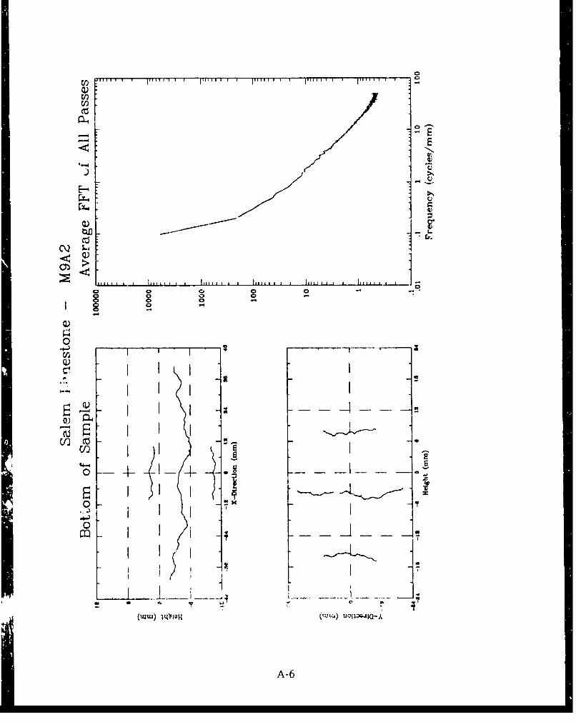
0

r+J

';" I I I I

cuV)

(tutu Ifbo I'w volal1 l

A-6

00

C\21.4

• .q

11~1 I 1111 a l elHt pwm 111141louip p .

0 0 0 -- 70 -'

-I [ I I -"4

E _ I I 0

S I II I - 4 -

- --

oI~ I I I~

4A-7

i IIII

0I j0 ll j u" .- T - -r

E-4E

0 .

~~4D

Q))

Q

O.4 ,.... I p

0 - -

0 0

SI

I UM Iq~* (C0)InDII

A-8

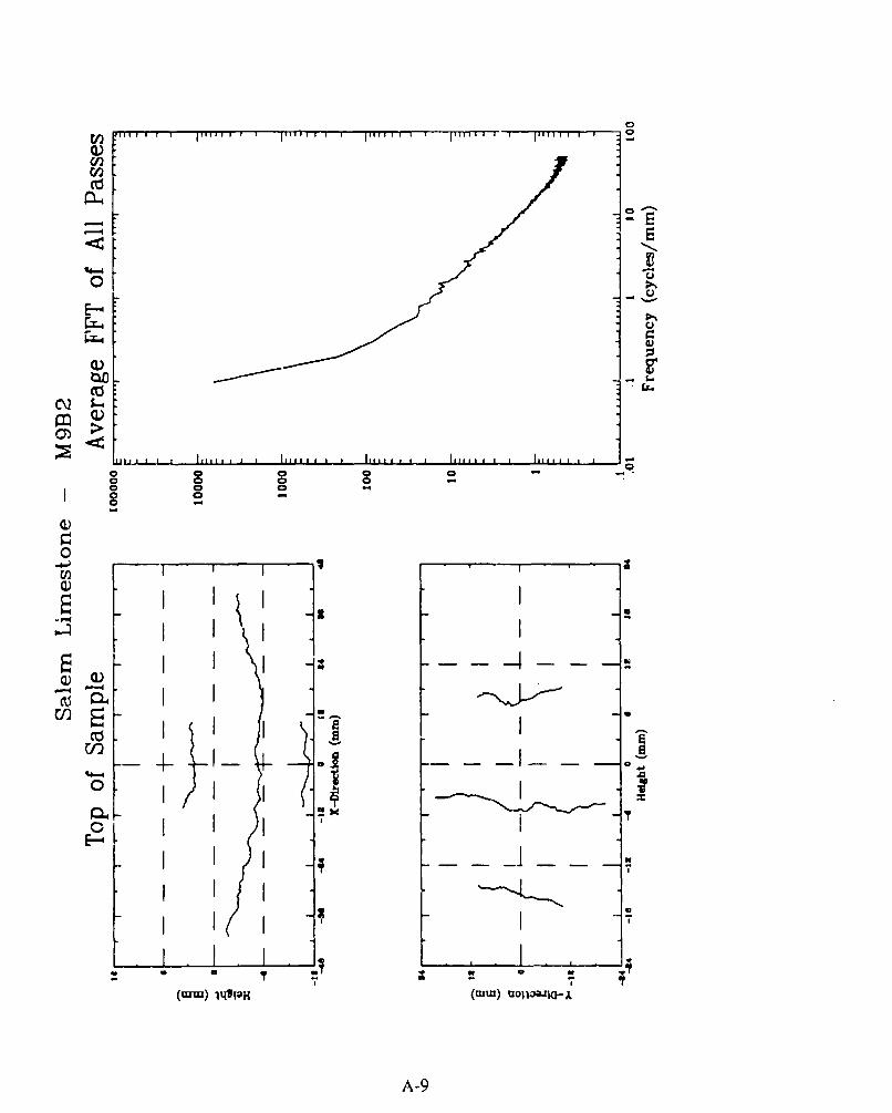
00

E-E

CUU

C\2

CI•

N-9

0 _ _ _ _ _ _ _ __ _ _ _ _ _

(Ulm 102 (Mn I01a*J

A-

C°i,

00

""-

0 > '

0

SI

0t)

0>4

0~0,

o x

00

SI I I1

I I ,,

, I , I . I ,-I a

(turn) H (UJa3) uo•J132I-4k

A-10

0

C\2

134-

co 00

cfcI

0

A - I

o 0 --

o 0 I

8 -

,, 7I I

I I I I IIII

00

U-4

Li;.

(um lq4)uil-ja,

I. . . ". . ... ... . . -

o

o - •

I I

. I I I IS' I I

II

I• " - -- i4-S... I-

- a

,*- --- I, ,~

S ID o"'""(I ru Iqlo (I)u l•.t• ,

A-12

2 I .. . .i i ...... . .I I . .. II I I I -

CI)

co

E,-4ýT4

00 0l 0I0

P--4

c o 0lI

A-13

*I p h h I I .. .I I I l l I 1 1 1 I IIIIIII

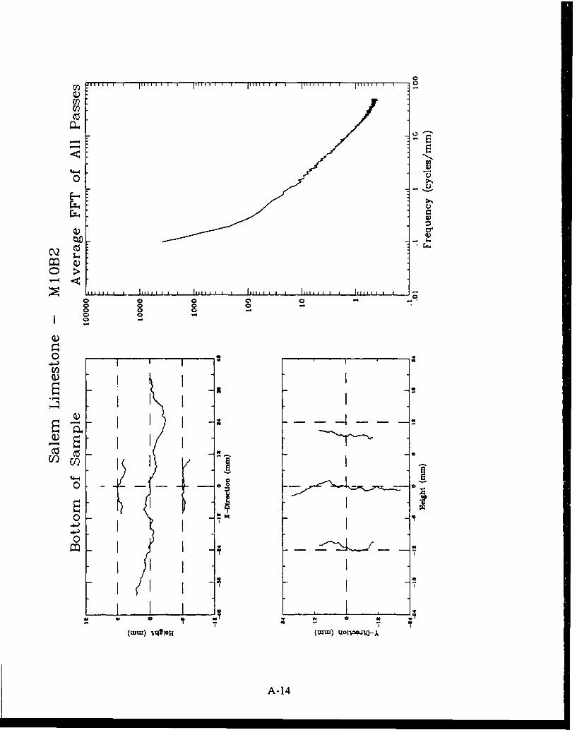
a

II III rillI i ' '

Q,)

-E

0 >

I lilil. I 11111 I I, I.. , , I

SA-1

00

'4A- 14

C\2

*- E

0>- - .4

-

-4

-

0>

§ o 0 0 -

0 0

(mm

A- I I I 1S2I I , 1 =---

oI IK I I

U) i-4

o Io I ' I r

I IIjI

APPENDIX B

UNCONFIN"EP COMPRESSIVE TESTS WITHPOST FAILURE RESPONSE

Test ID Page

M12A1 B-2

M13B1 B-3

M13C1 B-4

M13E1 B-5

M13GI B-6

M13FI B-7

B-1

Unconfined Compression Test (M12A1)Salem Limestone (SL21-B7)

o0I 1SRadial i Axial

Q) 40

u0)

Q)

4-4

• , 20

U)

-1.5 -1.0 -.5 0 .5 1.0

Strain (%)

0

-.5 -

"• -1.0 -

-1.5

0 .5 1.0 1.5 2.0 2.5

Axial Strain (%)

B-2

Uncunfined Compression Test (M13B1)Salem Limestone (SL21-B11)

60 I I I

Radial I Axial

Q) 40

S• 20 /

-3 -2 -1 0 1 2

Strain (7o)

-4

co

-2 -

3-0 2 345

Axial St~rain()

B-3

Unconfined Compression Test (M1 3C 1)Salem Limestone (SL21-B23)

60 I 1

Radial I Axial

Q) 40

U /u

*~20

01_a)

-) -2 -1 0 12

Strain (%)

0 - -,,I -- 2

"4-)

0 1 3 4

Axial Strain (%)

B-4

Unconfined Compression TesL (M13EI)

Salem Limestone (SL21-B22)

SRadial Axial

o4

";" 20-

-3 -2 -1 0 12

Strain (g)

'A

0 1 2 3 -

1 I I St__5 T

Unconfined Compression Test (M13F1)

60 Salem Limestone (SL21-T7)

Radial g Axial

S40 -S40

4-4

(J2_4

-1.5 -1.0 -. 5 0 .5 1.0

Strain (%)

0|

-4

.5 1.0 1.5 2.0

Axial Strain (%)

B1-6

Unconfined Compression Test (M13Gi)Salem Limestone (SL21-T6)

80

Radial i Axial

•) 40

C)

-. 5- 1.0 -. 5 0 .5 1.0

Strain (%)

0 - .

',-

CO

-1. -. 0 -. 0 1. .0 1.0

Axial Strain (%)

B-7/B-3

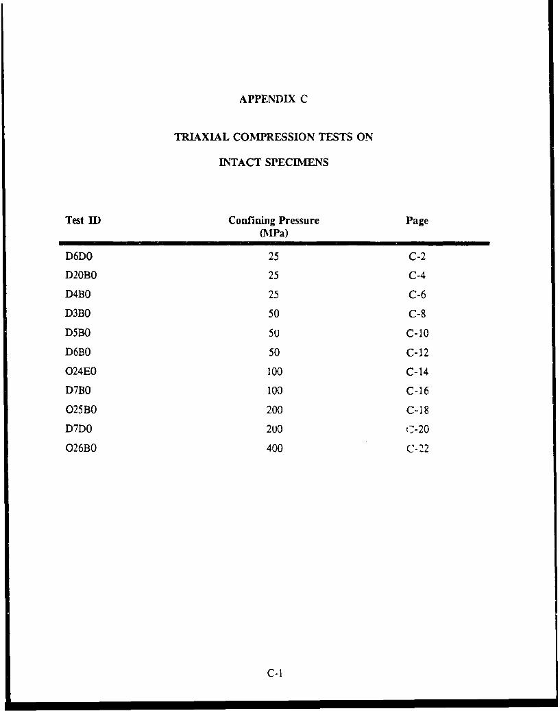
APPENDIX C

TRIAXIAL COMPRESSION TESTS ON

INTACT SPECIMENS

Test Hi) Confining Pressure Page(MPa)

D6DO 25 C-2

D20BO 25 C-4

D4BO 25 C-6

D3BO 50 C-8

D5BO 50 C-10

D6BO 50 C-12

024E0 100 C-14

D7BO 100 C-16

025B0 200 C-18

D7DO 200 C-20

026B0 400 C-22

C-I

Triaxial Compression Test (D6DO)Salem Limestone (SL20-T1B), Uconr = 25 MPa

150 - I

Radial i Aiial ......... Top- - Center

Bottom

) 100

'4-44.4"" 50

00

Q/)

-12 -6 0 6 12 18

Strain (%)

150 1

04

~) 100

AlA

.4-4

S 50

4.)

00 5 )0 15 20 25

Strain Difference (%)

C-2

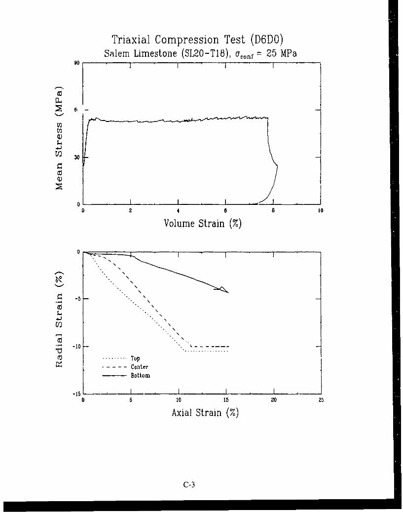
Triaxial Compression Test (D6DO)Salem Limestone (SL20-T18), aconf 25 MPa

gO " I I

S8, -

90

$-4

30

qj

0 2 4 8 8 10

Volume Strain (%)

0 I

NN

N\4-)

So ...... . .........

cr --------- TopS~Center

Bottom

-15

0 5 1O 15 20 25

Axial Strain (%)

C-3

I I I I I I II I

Triaxial Compression Test (D2OBO)Salem Limestone (SL20-B14), Oconf 25 MPa

150- I I I

Radial i Axial Upper Quarter......... Lower Quarter

Q) 100

Q).4-4

S50

-12 -6 0 6 12 18

Strain (%)

150

q) 100

s-IO

C)

#4-4".,_ 50

Q)

00 5 10 15 20 25

Strain Difference (7)

C-4

Triaxial Compression Test (D2OBO)Salem Limestone (SL20-B14), aconf = 25 MPa

90" I 1

60

A -4 -2 0 2

Volume Strain (%)

0 ......... . . I- . i"I

Upper QuarterS......... Lower Qu&Arer

- 16 1 1 1 , - I - -0 5 10 15 20 25

Axial Strain (%)

C-5

I5- III I

Triaxial Compression Test (D4BO)Salem Limestone (SL20-T21B), ocor = 25 MPa

150 .. -,

Radial Axial

0.4

Q) 100

Q)

'4-4

S50"0• 6

CO

-12 -8 0 0 12 18

Strain (%)

•) 100

15

4-444-4"0 50

U)

CI)

05 10 15 20 25Strain Difference(%)

C-6

Triaxial Compression Test (D4BO)Salem Limestone (SL20-T21B), uCcon1 1 25 MPa

90- I .

6 0 -

qI)

q) 30-

0-8 -4 -2 0 2

Volume Strain (%)

-5-

L..,)

15Axial Strain()--

C-7

Triaxial Compression Test (D3BO)Salem Limestone (SL20-T16A), UcorIC = 50 MPa

, 150

0

G)".4

I4..

" 50

-12 -5 0 8 12 1

Strain()

150

too

1-.

Q)

~ 50

0 10 15 20 25

StraiD Difference (%)

108

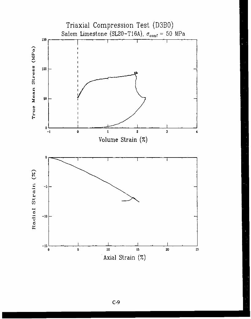
Triaxial Compression Test (D3BO)Salem Limestone (SL20-T16A), rconr 50 MPa

S 100Q)

E-,

-1 01 2

Volume Strain()

- 15 . I ,.!0 5 10 15 20 25

Axial Strain()

C-9

0 III

Triaxial Compression Test (D5BO)Salem Limestone (SL20-B21), uorI = 50 VPa

150 1.-- -

a. Radial i Axial

C)

100Q)

-e--i

S 50

L-4wt

-12 --6 0 12 18

Strain (7)

150 -I- - I15.0

CO

ao

1I00 - . -- • --

I.-

C 50Q;

F• 01 I 1,I, _ l

0 5 10 15 20 -5

Strain Difference (%)

c-10

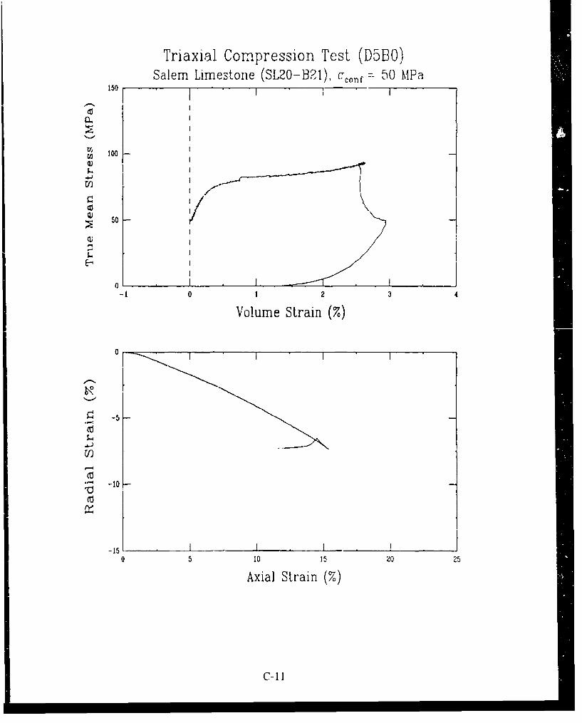
Triaxial Compression Test (D5BO)Salem Limestone (SL20-B21), o 50 MPa

t /

w 50

101

o I_, 1j- 0 1 2 3 4

Volume Strain (7)

S " I I 1

S-5

'• -10 -"0

-15 I I ,I _ ,0 5i 10 15 20 25

Axial Strain (%)

C-11

Triaxial Compression Test (D6BO)Salem Limestone (SL20-B13), uor = 50 MPa

. 150

(L PfadA i Axial

100 ...... TopS~ Center•. Bottom

•} 50 -'L4-

to

-12 -6 0 6 12 18

Strain (%)

1500C)

ro- =

•o 50Q)

0 5 10 15 20 25

Strain Difference (%)

C-12

Triaxial Compression Test (D6BO)Salem Limestone (SL20-B13), o = 50 MPa

100 -

Q)

1.44 1

-2 -2 0 3 2

Volume Strain (%)

0,. -- - -:.< " .,

(0

C') -5 --

......... Top

CenterBottom

-15I, I _I ,I l .0 5 10 15 20 25

Axial Strain (%)

C-13

Triaxial Compression Test. (024E0)Salem Limestone (SL20-T9), Conf = 100 MPa

S300

Radial i Axial

200

Li

V)

Strain(

300U) -20 -B08 21

1~ 00 -

I00

0 51000202

Strain Difference()

C-14

Triaxial Compression Test (024E0)Salem Limestone (SL20-T9), rconr = 100 MPa

300 I

(.

S 200

L40.-)

100

Q)

0 I , Ij-2 0 2 4 6 8

Volume Strain (%)

0

"- -0

10 i

-15 I , I0 5 10 15 10 25

Axial St.rain (%)

C-15

Triaxial Compression Test (D7BO)Salem Limestone (SL20-T19), aonr = 100 MPaS300 ',

SRadial i Axial

200

g.-4

S 100Q)4.,

C,)

E- 0-12 -6 0 6 12 18

Strain (%)

300

200

4)

Sloo

Q) U 100C)

0 5 10 15 20 25

Strain Difference (%)

C-16

Triaxial Compression Test (D7TBO)Salem Limestone (SL20-T19), Uconrf= 100 MPa

300

S200

0) 100

E-

-2 0 2 4 6 8

Volume Strain (%)

S-5 -

opd. -0

0 5 10 15 20 25

Axial Strain (N•)

C- 17

Triaxial Compression Test (025B0)Salem Limestone (SL20-B9), 0 cont-. 200 MPa

-, • oo- - I

0Radial i Axial

"400Q)U

400

Q)

0- o t, I, I-12 -6 0 6 12 18

Strain()

60-

r 400

'I,

• 200

Q)

0

-15 -0 85 20 25Strain Difference

C-18

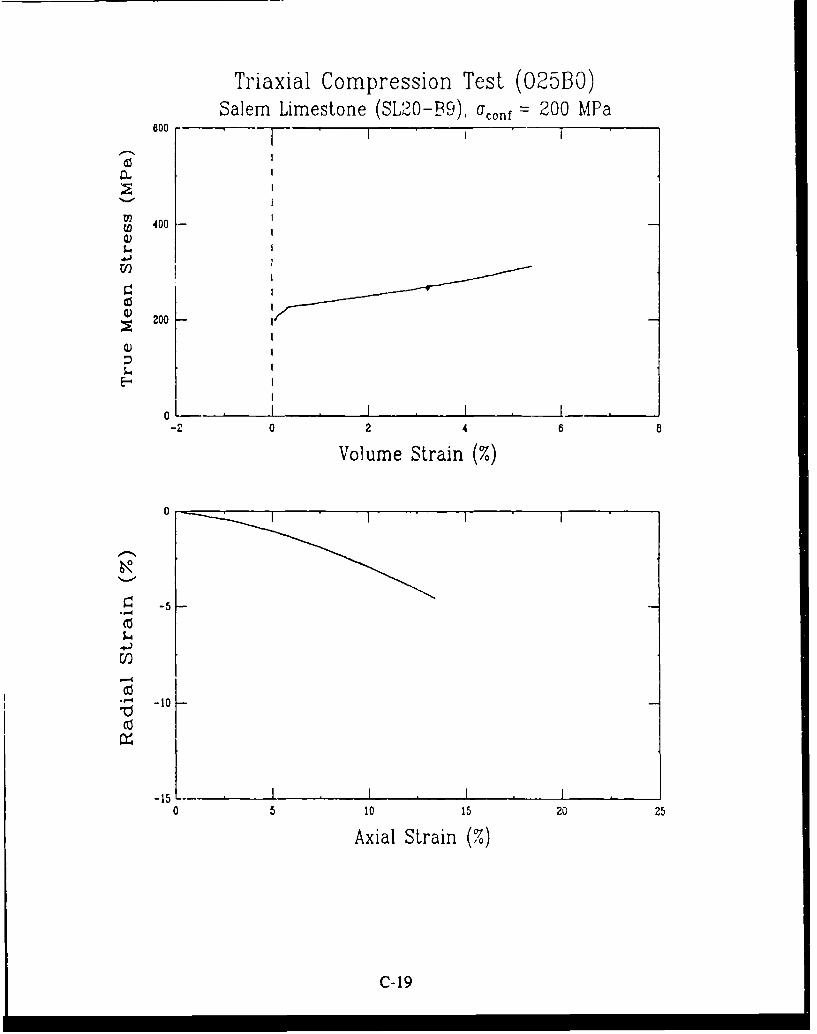
Triaxial Compression Test (025BO)Salem Limestone (SL20-B9), uonr = 200 MPa

600 - ,'II"

(D 400

9)

200)

0)

-2 0 2 4 6

Volume Strain (%)

0

S-5 -

"10 -O -

0i -. _I I , I

0 5 10 15 20 25

Axial Strain (%)

C-19

Triaxial Compression Test (D7DO)Salem Limestone (3L20-T13), aConf = 200 MPa

.- 00 1 10

Radial Axial

0

-12 -6 0 12 18

Strain()

400

.4-

m 200

C)

S-A

5.4

-12 -I 0 1 1_1I

0 5 10 15 20 25Strain Difference

C-20

Triaxial Compression Test (D7DO)Salem Limestone (SI20-T13), Uor,, = 200 MPa

600

S400 -

(U

S200

F--

0-2 0 2 4 6

Volume Strain (%)

0

,•-5

U)

.,w-10

-15! I ,-I. - -. . .. ._ _

0 5 10 15 20 25

Axial Strain (%)

C-21

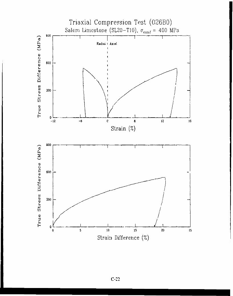
Triaxial Compression Test (026B0)Salem Limestone (SL2O-T1O),_c~o11f 400 MPa

I-I " --1 ------ "

Radiai i Axial

at)

600

300 /

0-12 -6 0 6 12 18

Strain (%)

,i.,,..•0 900 I I

900

C)

S600

'I-.

- K/S00

0 • ,!, . II ,

0 5 10 15 20 25

Strain Difference (%)

C-22

Triaxia] Comprcssion Test (026B()Salem Limestone (SL20-T10), •onr = 400 MPa

& .0 I I .

300w

-2 0 2 4 G 8

Volume Strain )

0

S-0

-1 I , ,1 '

o 1O 15 20 25Axial Strain (%)

C--3' C-24

APPENDIX D

HYDROSTATIC COMPRESSION TESTS

Test ID Page

NLAO D-2

Y15AI D-3

Y15B1 D-4

Y16AI D-5

Y17A1 D-6

Y20A1 D-7

D-1

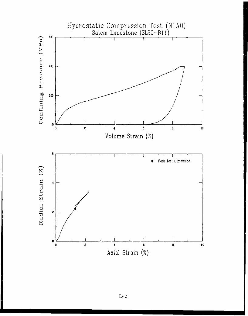
Hydrostatic Compression Test (NMAO)Salem Limestone (SL20-Bi 1)

-*' 600

ý--l

400 -U)U)

200 2-.4.,.-4

0

0 2 4 6 8 10

Volume Strain (%)

6 - I I

0 Post Test Dimension

.- 4

"*' 2

00 2 4 6 8 10

Axial Strain (%)

D-2

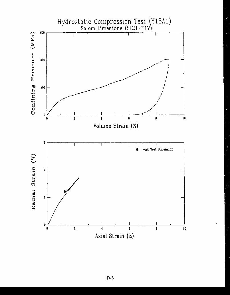
Hydrostatic Compression Test (Y15A1)Salem Limestone (SL21-T17)

0U

'124 10

Volume Strain()

S I I I

0 Post Test Dimnension

4

0 I

0 2 4 8 8 10

Axial Strain (7)

D-3

Hydrostatic Compression Test (Y15B1)Salem Limestone (SL21-T1O)

'-~ 600CO

400

r.,Cl)

0-

"-4--

0 0

0 2 4 8 8 1o

Volume Strain (%)

0 Post Test Dimension

CO

10

"1 2

CO

00 2 4 6 8 10

Axial Strain (%)

D-4

Hydrostatic Compression Test (Y16Ai)Salem Limestone (SL21-B12)- 600 • "•"

CO I

400 -

200

00

0 ot024 6 8 t

Volume Strain (%)

8-F SI I -

I Post Test Dimension

4L-

0 I I ,I ,I,

0 2 4 8 8 10

Axial Strain (%)

D-5

Hydrostatic Compression Test (Y17At)Salem Limestone (SL21-B19

600

400 4

M 200 -

44-4r. -

00 2 4 6 8 10

Volume Strain (%)

6 Post Test Dimension

"'• 2

0

o0 . I I _, I _ _[ _0 2 4 6 8 10

Axial Strain (%)

D-6

Hydrostatic Compression Test (Y20A1)Salem Limestone (SL21-T22)

- 00

400

200

010 2 4 6 8 10

Volume Strain (%)

s ,1 -I " I

9 Post Test Dimension

- , 4

U)

S 2

0 I I0 2 4 6 8 10

Axial Strain (%)

D-7/D-8

APPENDIX E

LUNIAXIAL STRAIN TESTS

Test ID Page

Y23A 1 E-2

U18AI E-5

U19A1 E-8

E-1

Uniaxial Strain Test (Y23A1)Salem Limestone (SL21--T19)

900 I ' I

6.,: 00--

'• 300-

o 3 6 9 12 ,

A•xial Strain ('7)(IV,

:• 600

1 900 -3-- /1

M

<l /:.///

0 300 600 900 1200 500

Confining Stress (MPa)

E-2

Uniaxial Strain Test (Y32 2-)Salem Limestone (SL20-T'19)

00 I

--- -" 2 00 -- --

0 100 200 300 400 ýi00

Mean Stress (•IPa)

21 c0

10

S-4

S1 0 _00,.0 300--C _0

Volume Stress (M)

E-3

Uniaxial Strain Test (Y231,)Salem Limestone (SL20-T19)

S 600L

4.)

I I

00 3 6 9 12 1

Volume Strain ('0)

E-4

Uniaxial Strain Test (U18A1).Salern Limestone (SL21-B14)

900. -

6C .

, i

"" 6 12 150 300

Axial SEtrain (;

9C0

6:r

600-

< /

/ ,

30 3 6 90 12

Coninin Stress (Ml%)

9F-5

,, I

* / /

× ,* //

< //

0 3CC 600 900 ,,.•, :500

Confining Stress (MPa)

F:-5

Uniaxial StTrain Test. (1B71)Salem Limcsione (SLO.-B14)

300 I

oj 200[ J1

SicoK1//

100 200 30040 O

Mean Stress (MPa)

i ,200-

- -- 'I

-E-6

0 0

- 2O ii -

CC I _ __ __

0 3 6 9 IZ 15

Volume ¶•rain (%)

E-6

Salem Limestone (SL2O-B14)900

a--

,o 1 1

' I /

-,-.7'

0 3 6 9 12 15

Volume S~rain (%)

E-7

Uniaxial S-train T est (U19A1ASalem Limestone (SL21-T20)

900

600-

CC

-Ju300

I! I0 ,I I ,: •:

o 3 6 9 12 15

Axial Strain (%)

900 I

600

"- 00 ~ 20 w9010

I ///r,-E .

r• ooL- / /

0 300 500 900 1200 :500

Confining Stress (MPa)

Uniaxial Strain Test (U 19A1)Salem Limestone (SL20-T20)

00V -

J) 0

"5 '.00 r -

I• o I! 7 J/t I I , _

o 100 200 300 400 500

Mean Stress (MPa)

200-

o0

UE-9

J2 I 10 3 6 9 12 15

Volume Strain (%)

E-9

Uniaxial Strain Test (U19A1)Salem Limestone (SL20-T20)

900. I I I I

S600 Iw i

No07

0 3 6 9 i2 15

Volume Strain (%)

E-10

APPENDIX F

ASTM/ISR INTERLABORATORY COMPARISON TESTSTest I D Material Test Type

G2SF' Barre Granite Unconfined F-2G28H1 Ba-re Granite Unconlined F-3G2SG I Barr, Granite Unconfined F-4G28EI Barre Granite Uncilnvned F-5G2SDI Barre Granite Uriconjined F-6G28B1 Berea Sandstone LUnconfinc F-7G2NAI Berea Sandstone Unconfined F-9G28GI Berea Sandstone Unconfinej F-iOG27F 1 Berca Sandstone Uneonfined F-1iG27A I Salem Limestone Unconfincd F- 1G27 81 Salem Limestone Uncon'In.. F-13G27E1 Sah:m Linesione Unconlincd F-14G2-C I Salem LUmestoie Unconfined :.!5G23D 1 Salem Limcstone Unntined F-16

'9Ai- Ter,n -,: Marble 'nc:trtincd F-! 7G29C L T.nnessce Marble Unconfincd F-i gG29E1 Tennessee Marole Unconfined F-! 9G29Di Tennessee Marble Unconfir-ed F-20G29R, Tennessx Marbie Unconfired F-2 I' E3 Larre Granite 1O MPa Triaxiai F-22U3B3 Barre Granite 10 NIPa Triaxiai F-:3U2F3 Barre Granite '0 MPa Triaxial F-24U3A3 Barre Granite 10 MPa Triaxial F-25U3B3 Barr-- Grante 25 M ia Triaxial F-2t,U3C3 Barre Granite 25 MIPa Triaxial F-27U3D3 Barre Granite 25 MPa Triaxial F-28UJA3 Barre Granite 25 ,MPa Triaxial F-29UL4B3 Barre Granite 40 NPa Triaxial F-30U4E3 Barre Granite 40 MPa Triaxial F-31U4C3 Barre Granite 40 MPa Triaxial F-32U4D3 Barr i-ranite 40 %IPa Triaxial F-33Y26C3 Bercu )andstone 10 \1Pa Triaxial F-34Y26D3 Berea Sandstone 10 MPa Triaxaial F-35Y26A3 Berea Sandstone 10 MPa Triaxial F-36Y26B3 Berea Sandstone 10 MPa Triaxial F-37Y27A3 Berca Sandstone 25 .IPa Triaxial F-38Y26E3 Berea Sandstone 25 MPa Triaxial F-39Y27B3 Berca Sandstone 25 MPa Triaxial F-40Y27C3 Berca Sandstone 25 NIPa Triaxial F-alY27'E3 Berca .d,•ao 40 MPa Triaxial F-42Y27 D3 Berea Sandstne 40 MPa Tr axial F.43Y'3Al Berea Sandstone 40 NIPa Tr:axial F44Y2,F3 Berca Sandstone 40 MPa Triaxial F-45Y28D3 Tcnnesnee Marble 10 NIPa Tnaxial F-a6Y28B3 Tennessee Marble 0 MIPa Triaxial F-47Y28C3 Tennessee Marble 10 MPa Tnaxial F-48UIA3 Tennessee Marble 10 MPa Triaxial F-49U 11B3 Tennessee Marble 25 MPa Triaxial F-50U I E3 Tennessee Marble 25 MPa Triaxial F-51U IC3 Tennessee Marble 25 \IPa Triaxial F-52U I D3 Tcnn'ssee Marble 25 MIP'a Triaxial F-53U2C3 Tennessee Marble 40 M IPa Triaxial F-54U2A3 lennesscc Marble 40 M Pa Tiiaxial F-55UD3 Tener,cssee Marble 40 % Pa rriaxial F-56U8B3 Tennessee Marble 40 MPa Triaxial F-57

F-1

Lnconfined ComIDression Test tG28FI)Barre Granite (!jG/ 91," 1-7)

N00

Radial Xxial

S2O0 - //

'0

/

Al S

F .2

*-[ L.________-______

--.4 -,2 0 .2 .

Strain (%•)

I

I N

- I • I

0.1 2 .3 5

Axial Strain (%)

F-2

Unconfined Compression Test (G28HI)Barre Granite (BG/'91/2-15)

300 I

I Radial Axial

,• 200 • -'

® \ /

* r100,\

*s I

-4 -2 0 .2 .4

Strain (%)

0

.z -.1H-"

-.3 I i ,,,_0 .1 2. .3 .4.5

Axial Strain (%)

F-3

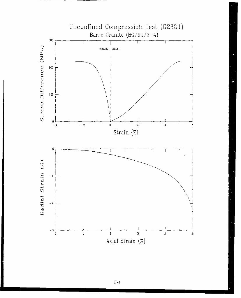
Unconfined Compression Test (G2BGI)Barre Granite (BGi"'91/"3-4)

300 . ......

Radial i Axial

S200 -

*10

-.4 -.2 0 .2 .

Strain()

2•

F-44

"- .

• 'I

-3 o , I , __ i,'-. 1. .2 .3 .4 .5

AilStrain (%)

o = , , lF-4

LUnconfied Compression Test (G28EIBarre Granite EG, 91/5-)3 0 0 ,

.i R a d ia l .A x ia i

757

// c

V \u0 / -I-, //

- .2/*- icL- I "/

/

-. 37

'." 0

-4 -. 2 0 2Strain ain

,1 K - I

.,s I I-3

""0-. ._.- . ._5

"AxalStrin(!

nUnconfined Compression Test I Gs 8DI)Barre Granite BG/91,6-8)

300, II

I Radial .Axial

. zoo •\/o, I

'• :OI_ '///

- 0I',, i/

/ I

200-. , 0 .4 .2

"Strain (7)

0-

"° I

.,. -. |r----

-~ I

-.31 ' i J_30 .1.2 .3 ., .5

Axial Strain (%)

F-6

Unconfined Compression Test (G2B.63)Berea Sandstone (BS/'91/9!-7/"1)

•e - = - I - I t

I Radial Axial

;30

-- 2 0 .2 .6

Strain()

1\0

-- I

"" 0 --. 4 6-- 1

0\

.6 8

Axial Strain ()

11-7

Lnconfined Compression Test (G?8A1)Berea Sandstone (BS/91//2-15)

90 i I I

IMI

.• ,, Radial I Axial I

-0 .2

S''train ()

0 .24.. 81

F-

..- - t .'-

I,

,- ' I

- 4-2 .0 .6 .4 6

AilStrain (%).

-F-8

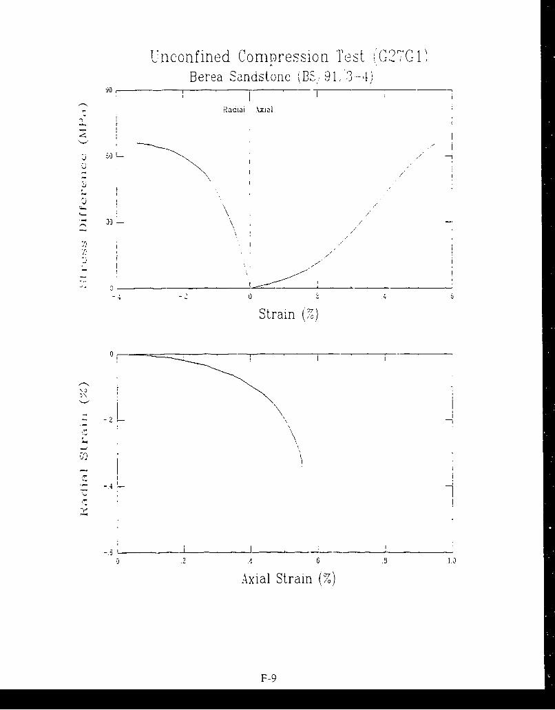
Unconfined Cornmression Test , C-27C, 1Berea Sandstone Bz,. 91, 3-4)

90,

Radiai U.jxal

3-3

2)

1.

- I

I--

.- 3,)- '

* I .. /

o I

-- -2-- N \

.'\

"I I

0 .2 .4 6 .5 1.0

Axial Strain (%)

F-9

Unconfined Compression Test (iCG3Ci)Berea Sanastone (BS.;'91,A4-i)

90

P:.didi kxial

Q) 60 -

t ) i

L&-4 /"" 30 -'

. /7

-. 4

ci'\ _ _ _ _ _ _ _ _ _ _I_

-4 -2 02

-. 6

Axial Strain

F-'10

Unconfined Compression Test (G 9TF1)Berea Sandstone (BS"/91/4- 16)

,Z Radial Axial

2.•j 6O=,•/

/

o \ /

3"- /

'\, /"

* .

51-o I , ,

Strain (%)

0 " ''

717

.- -4--

I--)

-6 [ 6

Axial Strain()

..... 1 -i \

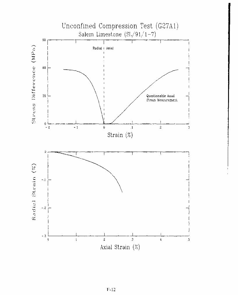
Unconfined Compression Test (G27Al)Salem Limestone (SL/917,1-7)

90 I I I

I Radial i Axial

C) 60 -

n' 0- Questionable AxialStratn Measureme:nt.

0

-,3

- -.1 C .1 .2 .3Strain (%)

o . - I2,

Irl

unconfined Compression Test (lG.,,7B1)Salem Limestone (SL,"91,"2- 1tI

S' a d ia l A x ia l

"11

[. 4 I

/

//

-, I

-2-.i 0 .1 .2

St.rain (%)

o-. ... _.. ,

----.....

-- O. 1 .- ,,

Axil Srai,(,

P*-\

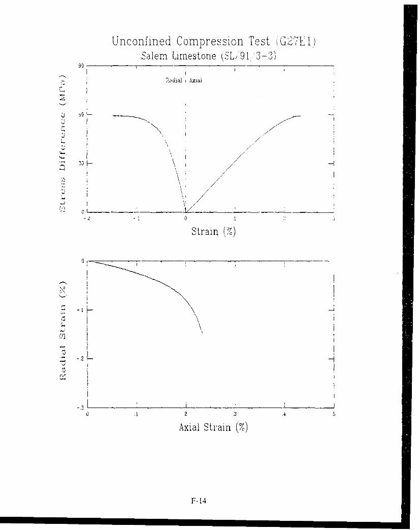
Unconfine(d Compression Test tG27EE11)Salem Limestone (SL,,91.3-3)

Z diad i W-ai

.•Ax•ial "Strai n (,

----- 4

S• /

*- 33+-\/-- /-

"* ,, / •-I /• - , 0 ..

Strain (g)I

- I

_.9 -_____ _ _

C .1 2 .3 .4 .5

Axial Str'ain (%)

F- 14

Unconfined Compression Test (G27C1)Salem Limestone (SL,/91/ 13-20)

I I.I'

Radial Axial

S, ttC - .

-. 3C

r 'I

-.2 -.1 0 .3 .3

Strain (%,

F- 15

,J 2

.' 5

Axial Strain (%)

F- 15

Unconfined Compression Test (G27D1)Salem Limestone (SL/"91,/4-15)

90 F

I Radial Axial

60 I

C..

S I \1

-.2 -. 1 0 1 .2 .3

Strain (g)

..1 -4.

Axial Strain()

F- 16

Uncorifined ComDression Test %G29A1!)Tennessee Marbie TMt/ .11, 2-19)

150 ;I

I Radia Amxi

-- I.0 - ,/

2 /.

Axi-a " I

5F- 17I /

I /

3. /

-. 2 -"0 .12

Strain (%)

S- I-~ I

.- ' -. t--

F-1

Unconfined ComnDression Test (G29Ci)Tennessee Marbie JTMi 91,,3/ 2- B)

4[0

I ,acijal Ax ial .ta i

F-1/8

- I

.\ /

r•-4 ,

. I I ,

I /

-.2 3 .1 .

Strain (%)

- I

-. 1 I ,.___ _ _ __ _ __ _ _.__ _

0 .1 2 3.45

Axial Strain (%)

F-i S

Unconfined Compression Test (G29E1)Tennessee Marble (TM/91,i'4/i1-2B)

'C0

. Radial A ial ,I /

.2

I I

Oj i00OL- \ /"

110~

I I /

:1 /

L. -.2 -.1 0 .1 .2 .3

Strain (i)

-F'K

,-2-

'V,,

0 .. 2 .3 .4 5

Axial Strain (%)

F-19

Unconfined Compressio., Test (G29D1)Tennessee Marble (TM/i91/4i/2-5B)

Radial i Axial /

{5•• I0 -- I 7' -

I\ /

I I /

/Al .

,F -2 0,.9- I //

. Q -- . ... V . I

Strain (%)

I I

- I

. , Li,0.1 .2 3 .4

Axial Strain (Z)

F-20

Unconfined Compression Test G29Bi)Tennessee Marble (TMi 91, 4. 2-20)

S~ Ra61e, w;:'xal"

2

S'0 :o .- ..

Si ~/

"T' i /

Axtrain Str

~F-2

- I

I

0 1 .2 3 .4 .5- -

Axial St~rain (%) .

F-21

1Traxial Compression Test (U92E3)Barre Granite (BG/ 91i 1-IB), u,,onf i0 MPa

-\ Radial Axiai /

"". .. /i

_ I

I /I/

' 0 I"

-6 3 0 .3

Strain ,\%)

.1 I I

L4~

.I

Axial Strain (%~)

F -22

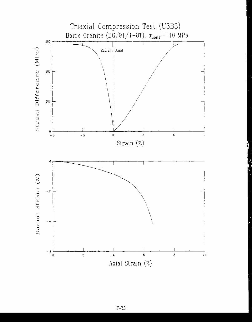
Triaxial Compression Test (U3B3)Barre Granite (BG/91//1-8T), cornf = 10 NIPa

300 -

Radial Axial /

-t \ /

- /o ..- /

2 , /I

200 7

0- 4 .

' '\ /'

*'- /

• -- 0 . .,.

Strain (%)

01 I I

"0 . [ .4.6.

Axial Strain (%)

F-13

Triaxial Compression Test (U22F3)Barre Granite (BG//91i/3-1B), aon-- 10 MPa

J00j

oRadia i Axial

200 I) /

- I /

I:-j

®I I "

6 I_-- I\ , /

i.00

I i/ /0 . /3.

-. ,'3 ~~-.3 0. 5"

Strain (i)

_ [. -.2 _.I

-.6 I ---.--

"0 2\408l

Axial Strain (Z)

F-24

Triaxial Compresslon Test i. .3-)

Barre Granite (EG, 92., 1 1-3), 1 ccnf 10300 , __I_ -•

"", Radial Axial

'-\

Go

StraMn2

Axial Strain (7%)

tF?

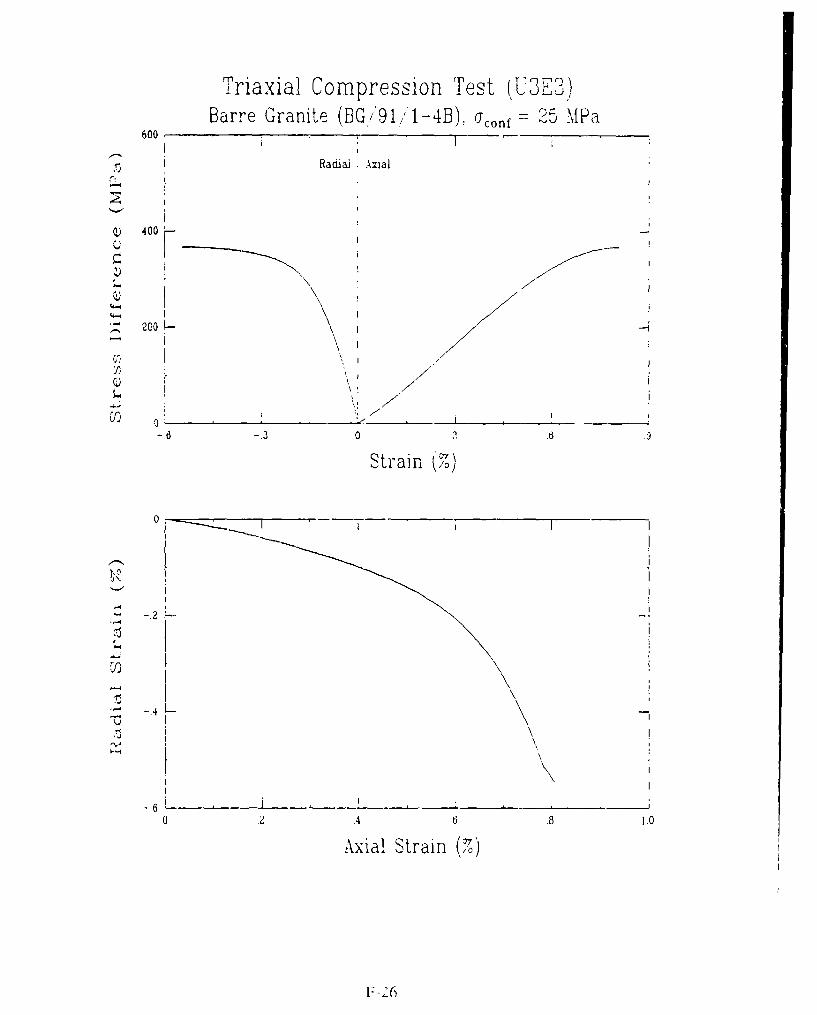
Triaxial Compression Test t U3E3)Barre Granite (BGi911t -4B). O0 ¢onf 225 IPa

600 - -

Radial .Uial

400[-

"4S

NoN

0) : I

• - -00 I , -i

I•I I,.

C O2 _ _ __.___ .. ,.____,.___ _ _ _ _ _ _.

-6 -. 3 0 .6

Strain (%

"I i

-. 4 L

-6~

0 2 4 6 8 1.0

Axial Strain (/7)

F -L6

Triaxial Compression Test (UL3C3)Barre Granite (BG/92/1/'1-24), uconf = 25 MPa

600 , i --

I Radial i Axial

404---

zoot

•/- o I • , ._ .I . _ _ _

-. 6 -. 3 0 .3 6 .9

Strain (%)

45 4_ _ i * W' I

0 .2 4 .6 .8 1.0

Axial Strain (%)

F-27

Triaxial Compression Test (U.3D3)Barre Granite (BG/92/1/1-27), cori= 25 MPa

600 '- ------ I I

I Radial i Axial

Q 43G L-

U -

200

.•

- -. 3 0 .3 .6 .9

Strain (%)0am

- I

I I I

0 .2 .4 .6 .8 1.0

Axial Strain().w==8

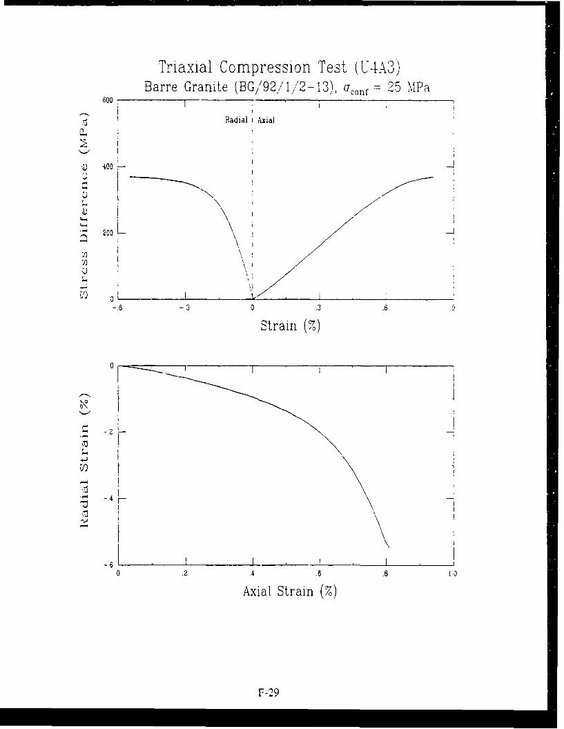
Triaxial Compression Test (U"4A3)"jBarre Granite (BG/92/1/"2- 13), Jcoff 25 MPa

600 I .

"" Radial i AialLL.4

- L,• 40 0 t--

S .2 4 .6

"F --.

- 6 - 3 0 .3 .6

Strain (%)

S2

-6-- I0.2 4 .6 .8 1.0

Axial Strain (%)

F-29

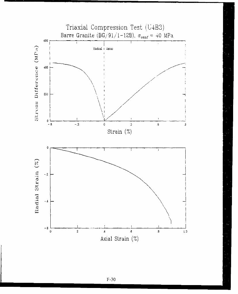
Triaxial Compression Test (U4B3)

Barre Granite (BG/91'/I-12B), acorjf 40 MPa

Hadial Axial

S400k-

"200k

-8 -.3 0 .3.6.

..,

\

AxtraintrainF-3

"-%l•/ I

I

• 0 .24 8,.

AilStrain (%)

F-30

Triaxial Compression Test (U4E3)Barre Granite (BG/91i2-17T), ucorlf = 40 MPa

600 1"1

Radial i Axial

Q.•• 400 •

"ý4 200 -

r 0

.6 -. 3 0 .3 .6 .9

Strain (%)

Of . I

-.6

S- --

I V

-.6 , I I .I0 .2 .4 .6 .8 l.

Axial Strain (o)

F-3 1

Triaxial Compression Test (U4C3)Barre Granite (BG/91/6-4T), goff = 40 MPa

6007

M Radial i Axial

Q) 400

4-41200

o L , Z.1

-.6 -.3 0 .3 .6 .9

Strain (5)

0

-.2 L

• \I

0 2 4 6 .8 1.0

Axial Strain (%)

F-32

Triaxial Compression Test (tU4D2)Barre Granite (BG,/921 1 -30.), (conf 40 MPa

600 ,-

Hacia I iAxiai

40) \00

- I

6-4

/.

.4

4-- 6 -. 3 03 3

Strain (%)

_F _

-. 6 I I

0 .2 .4 .6 .8 i•

.A xial Strain (%)

F-33

M -•26C3)Triaxial Compression Test '.26C3)Berea Sandstone (BS, 91, 1-), j 10 MPa

i 50,I

Radial Axlai

100

I0 io - \ ,/ /

/

:3)Sr i " /70

I /"

---- -------

.1 /

j/) ,I,/

*, I-, .

-o- 0 . .

Strain (S )

F -.234

z I\,,

_ I\

0 3.4 .6 .8 2,

Axial Strain (Z)

F -34

Triaxial Compression Test (Y26D3)Berea Sandstone (BS/"92/7/'3-3), 7,conf 10 MPa

150,

SRad ial i Axia l

4'

S"0 I -

"- I

'• 50 \"Q)

•3 0,

Axa Str-in

F-3

• ,,Or I

-.6 - 3 0 .3 .6 .

Strain (%)

- -z -I--

a2 .4 .6 .8 : 0

Axial Strain (%)

F-35

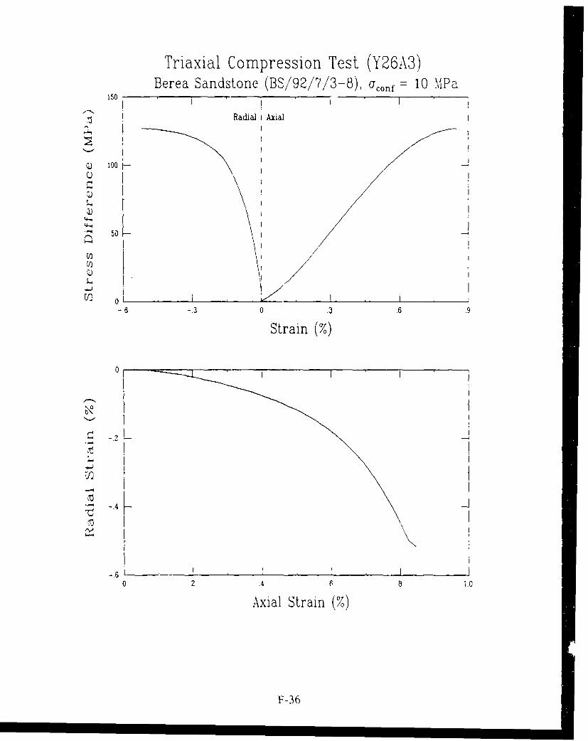
Triaxial Compression Test (Y26A3)Berea Sandstone (BS/92/7/3-8), Oconf 10 NMPa

150 I I I "

Radial i Axial

50-

c'' 0

I.3

U• •I....

- 6 -.3 0 .3 .6 .9

Strain (%)

6\0

I I , Io 2 .4 6 .8 1.

Axial Strain (%)

F-36

Triaxia' Compression Test (Y26E21Berea Sandstone (3S,,92/8.13 10

:50

Stai

-4-

3). UU- / -

\/

- /

LO oL /

-/ -- .

AxialiStrai

F ,

-,. .

xilStrain (5;)

0~1=-37

Triaxial Compression TeSt (I Y2,-V3'Berea Sandstone (BS,.91 ,' 9T, gconf Mp

300G

a k aI Ra~a1a .xial

I"

""- H0 -I" -,--o•o

Strain .)

3

\ ' ,

"3 6

Axial Strain (,)

Triaxial Compression Test. 'Y26E3)e, (B/1/92/,7,/ 35 ý, ,I a '.Berea Sandstone (BS!92 1-10), 7conf

300 ,

Radial Axial

',u 200

00

Strain A•

2. .3 1 L-

.6..

.- io-.6 -

',* I

- 3 . 9 .8 '.

Axiai ntral (,

F -3t-•

Triaxial Compression Test (Y27B3)Berea Sandstone (BS/92//7/2-16), Cr '25 MPa3co I ' 1 f

,Rdial Avial,,I . u a

I

1D 2 0 .

"Q) O00- --0

-8 -.4 0 .4 .

Strain()

-,T-

•" -. 3 -

- \

..

I V

-. 8 -.. . . . 0 . . . ..

Sxa ''train(%

I .3 ,6 .9 12 1 5

Ax ia ,tai (° .

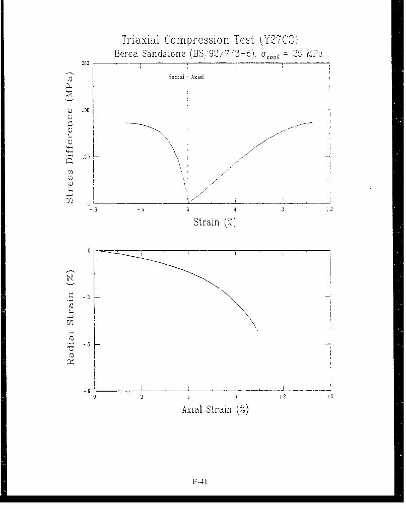
Triaxial Compression Test (Y'7C2;lerca Sandstone (BS, 92/7. 3-6,, 6 o 2. Mc>

300,

J RadiaJ Axial

SL

7)I0 • o --- 4,.._

'Strain()

F-4I

3j 6:, .1..1

AxialStain-(__

r-E-4 1

Triaxial Corrnpreaswnio TesL (YLTE3)Berea Sandstone (BSi91/i1--ST), Ocorif 40 MPa

300 '

,7:i Radia i Axial

S 200- -

f 4

1.) "

-3

Ai /I

-4F-42

ci: . I

-8 -.4 0 .4. :

Strain (,o)

S-3--

LN

.,.6.' 12 1

Axial Strain (%)

F-42

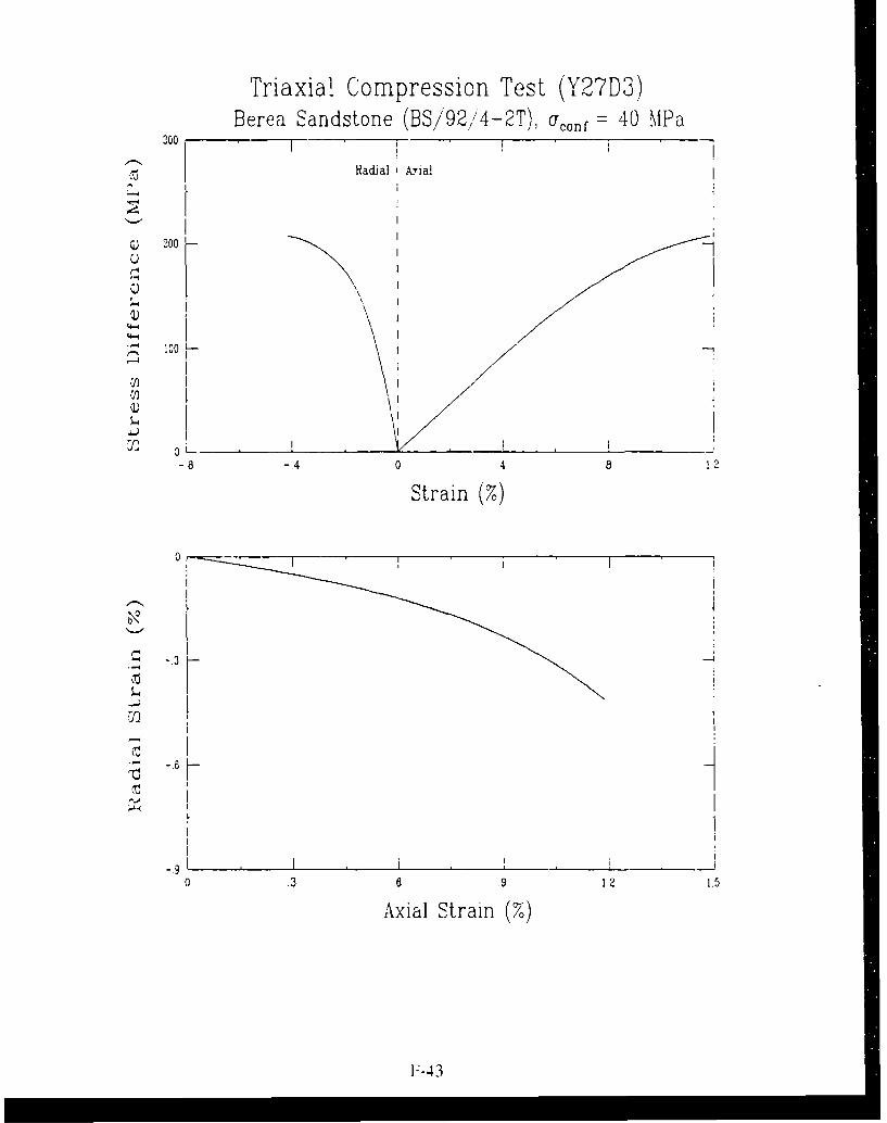
Triaxia! Compression Test (Y27D3)Berea Sandstone (BS/92i4-2T), Uconf u 40 Ma

300 I 0

Radial i Aial

C) 200H

14,

L- I

-" •'O -

-8 -. 4 0 .4 8 L2

Strain (%)

.- 4 ." -

0;;

- .3 I

I A- 9I ,I i

0 .3 .6 .9 1.2 1.5

Axial Strain (%)

F-43

Triaxial Compression Test (Y28A3)Berea Sandstone (BS/91/4-4T), U•ori= 40 MPa

300

,. Radia i Axial

Q) 1200 --

ci 0 1,\

0 .U• 0 -,J,-8-.4 0 .4 .8 1.2 •

Strain (7)

I-I

-.-.3 L--

-. 6

-, I

- .9 , . I I I.i,

0 .3 6 .9 1.2 1.5

Axial Strain (%)

F-44

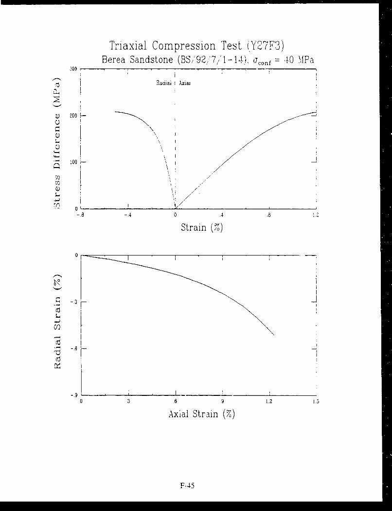
Triaxial Compression Test Y-2713)Berea Sandstone (BS,92,7,,'1-1,,. 1 conf 40 ,IFa

'00

200

0 L

IFI

AxiaStranai

~-4F-3-

_•

._

I

0 .3 .6 //,. 1

AilStrain (•)

F- 4

Triaxial Compression Test (Y28D3)Tennessee Marble (TM,/91 1 '1-4), i1 \I=a

200 ]-

Radial Aixial

.200-

-- I

- 00ko- \/-

I /

I.. _ 7/

- 4 -.2 0 24

Strain (%)

-.3o .1 2 . .5

Axial Strain (7.)

F-46

IMiaxial Compression 'Fest (Yt 3)-2 ,.Iennessee Marble (T.M,"91',.2 2-2B), c'conf - 1 a

' Rad'ai Axiai

x a t,•

T 7 1

- I

//

-o -2

Strainl H/

- -\

- -- I,

• [ "J

\ .

AxalS '\. f;

Triaxial Compression Test (Y28C3')Tennessee Marble (TM,'92, 5i/2-2), gconf 10 MPa

I Radial i Axial

02

CI

S

tI I

/ /

-2 /

I" I

-4 -.. 02

Strain (%)

- -lF-

'" -.2 '1

0 1 2 4 .

Axial Strain (%)

F-48

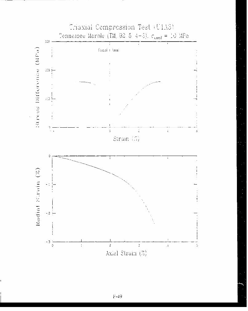
'1'nnessee :,la.Dle \TM. 92. 5 4-: - -' "

, '2

't x !\cC I A-3ia

-1 i

"s e I

3 I I a

F-49

71dXi: c~inres-liIeL kE1

ara, I,

-. S,

S•traint•

U ,-:

-4.1 --

F -5£)

T:iaxial Compression 'Fest (,U1 -E3\Te nnessee Marble (TM,/91..2i1-2), 2conf- 5 MPa

Radial A.xial

I I

- .

I /

- I I

, I-, A

AilStrain t~)

2 I I

'i' laxia! Compression Tesi. (I!IC3".ern"see A•'rue (,•T a.$ a, -2), ' =o~ 25' NIP

.£•R ~ 0i2( ,LA tl , , ,, , - , conf ,. .• t

-• ad a Axial

- "-

"-' 7F-

"* I, /

-u, -3 0 .3

Strain (2:)

- •I I

S- -- \-

-6 .

F-52

--- ' I N.' :-N .. ,

" " .'-. F-- "C ..- -- -

:Li

Ct -----

'1['m----

- , II

--,,-

- _.___. L__ - .. . J -- 4 *j: It

[--53

cr, uJ: *~..~a / *':CA U - - -,

A a

I ..

•.Iax•a- Compression Test (1Y"3-7':C ,. e,'• ,,[trblC (TM;'91 '4 8- (3• - -" ,P

alAxial

Stai

AI /

*1-5

J i

-• / i -

-, I.

z I

_ I'

"r i //4

T iCompression Test (U2D:3).ennes•le Marble JIM. 92,, ,, '- 92 .5 = ,Ie,,7 c u --I f '.Pai"

I-x ] I

_ _ _ _ ~h a Ixi _ .

'Strain (;

A X

- F. -50

.- I ' -

Sc.i. 4L_

;.: j: 5 (

. . l;: r•csin es ~ii

_'nr [es .e Mi .. M I92. • r, Q-5 4Q-.M;.a

S.-' , L ,I 'O--" -- -u ,

Straii

I" I

- /-, .

- I

-p

-u - -_- __

DISTRIBUTION LIST

DNA-TR-93-63

DEPARTMENT OF DEFENSE SANC.IA NATONAL -AEORATCRES

ATTi..' D!"V 921: L ~. '-;LL

A-ýCt ýNCED RESEARCH P.Ct.-CT AGENCY AT T N 0 OV 9 S L t

ATT.NJ DEFENSE SC.ENCES O:,iCE ATT, 92" C 'V StIlT"

ASSISTANT TO THE SEC,-RE'rARY OF DEFENASE OTHER GOVERNMENTA.TTN: EXECUTIVE A'SSISTANT

CENTRAL INTELLGENCE .:GENCYDEFENSE INTELLIGENCE AGENCY ATT,! DS`,R NED

A-TT'N! DB-6E2 ; DOPERALSKIATTN: DIW-4 DEPARTMENT OF THE INTERIOR

EFEt-NISE INUCLEAR, AZENCATTrN OPNA DEPARTMENT OF DEFENSE CONTRACTORS.AT4T SPSDA-Th. SPSC 0SENSENY AEROSPACE CORP

2 '/ ATTN. TITL ATTN. OBRARY ACr.... - '

DEFENSE TECHN:CAL INFOCc!.IAT! :.J CENTER .,'.,,NA YT C SERVI E S NC S-NEF

2 CY AT-T, DTICCC ATT.N: K BAKER --

DNA .ACO. zIAISON OFFICE APPLIED RESEARCH ASSCCIATES. iNCATTN. _.NALO ATTN. C J HIGGINS --

FEuD COMMAND DEFENSE NUCLEAR AGENCI APPLIED RESEARCH ASSOCIATES INC

ATTN FCTO 2 C' ATTN D CHITTY--ATTN. FCTOH 2 Cy ATTN: S BLCUIN

ATTh: FCTT G BALACI 2 CY ATTN K KIM

ATTN. 'l SUinM V AT"TM Vi S'- __;

DEPARTMENT OF THE ARMY AP-LiED R-ESEAR"CH ASSCCIATES. :r

AFrTN: R FRANKUL S ARMY CCRPS OF ENGINEERS

ATTN CERD-L 8DM ENGiNEERNG SERVERS :C--ATTN. D BURGESS

U S ARMY ENGINEER DIST OMAHAATTrN MROED-S H GAUBE SOEING TECHNICAL & MANAGEMENT SVCS. 'NC

ATTN- V M LEAVEN'S

U S ARMY ENGR WATERWAYS EXPER STATICN ATTNI: A W SPENCERATTN: C 0 N.OCRMAN ATTN: ROSS J WOODATTN: C EWES J K INGRAMATTN CEWRS-SD OR,. G JACKSON JR CAL!FORNIARESEARCH & TE-CHNOLOGY N`CATTN. CEWES-SE MR L K DAVIS ATTN J THOMSENATTN OR C BANKS CE'W'ES-GS A T.,iN: K KREYENH.AGENATT:. C ALBR!TTON -- "AT-h'. J BALSARA CEV'ES-SS.R lit RESEARCH IiiSTUTEATT,: J WARRINER IESGR-M ATTN: DOCUMI..ENIS L!BRARV

ATTN: RESEARCH -iBRARY ATT'N (i JCHNSON

ATTN: 'l MLLER 1- l Ii _;NR

DEPARTMENT OF THE AIR FORCE ATTr,N CLASS!FIED -.BRARY

A!R ;ORCE CTR FO, R STUDIES .- ANA.YSIS IA:COR

ATT',': AFSAA.SAI ATTN CYRUS P KOWLES

AIR UNIVERSITY LIBRARV KAMA;J SCIEN4CES CORP

ATTr, AUL-LSF ATTIJ. RICHARD KEE:E __

DEPARTMENT OF ENERGY K,','.!AN SCIENCES CRPATT !tj DAS;AC

LU.S ALAMClS ?:-,JAI '.,AI. LA.BOHATCR '\l l -I LS A S It '.

I , 1< I-

ONA-TR-93-63 (DL CONTINUED)

LACHEL AND ASSCC:ATES. NC uCNOS AFPJC.TNS '.T .

ATTN: C LINAriEN ATTN Al -.A"SO-. N~t J BECK ,. . ... ..

SCUT HXUST.. ' RESEARC-CH f"SZ.T'J-TE

LOCCON q C ASSDCCATES ATT'l A FR'' __

ATTN. L;BRAR'" A T T. -T,'-PcP

LOGICON R S C .S'-YCOIATES SC FITERNA TOk-L

.ATTN: V ,ALTON ATT'.: U GR..

L-C:,nCN P D ASStATES TTAN CORPORATZN ,THE

ATT'. C PIEN.UPG ATT"i _IBRA.FYATTN S S_-tSTEF

N.TS E:NG:,EE iN ATZTJ; I ..1 ITC

ATTN. A KEN'NEDYATTN. S SHORT 7T,, SPACE D-ZENSE SE.CTOR

ATTN. W ,iiAM:PLE.

PAOCIiC-SiERRA RESEARCH CORPATT`. H BRCCOL -TD. INC

A-T;J: E FCSTER

P AOIC- SIERRA RESEARCH CCRP-\ -_1.w . ,RllL -E Y' ! D N E C S S C !r ..C

AT'TN:0 GO - L... -"LNOE 550

AT-'h H LEII.IE

ATT•N: K DP'VATT JR ,EIDLINGER ASSOCIATES.,NATTN.' 1 SANDLER

SCIENCE APPLICATIONS :NTL CORP ATTh': !..I EARCN,ATTN DR .1 MCKAY

ATT..' TE•HN;OAL REPORT SYSTEM

IDost?