DeepMPC: Learning Latent Nonlinear Dynamics

for Real-Time Predictive Control

Ian Lenz1, Ross Knepper1, and Ashutosh Saxena1,2

1 Department of Computer Science, Cornell University. 2 Brain of Things Inc, Palo Alto, CA.

Email: {ianlenz, rak, asaxena}@cs.cornell.edu

Abstract—Designing controllers for tasks with complex non-linear dynamics is extremely challenging, time-consuming, andin many cases, infeasible. This difficulty is exacerbated in taskssuch as robotic food-cutting, in which dynamics might vary bothwith environmental properties, such as material and tool class,and with time while acting. In this work, we present DeepMPC,an online real-time model-predictive control approach designed tohandle such difficult tasks. Rather than hand-design a dynamicsmodel for the task, our approach uses a novel deep architectureand learning algorithm, learning controllers for complex tasksdirectly from data. We validate our method in experimentson a large-scale dataset of 1488 material cuts for 20 diverseclasses, and in 450 real-world robotic experiments, demonstratingsignificant improvement over several other approaches.1

I. INTRODUCTION

As robots perform tasks in the real world, they must be able

to handle a large variety of environments, objects, materials,

and more. Traditional robotics approaches which hand-code

controllers and models are ill-equipped to deal with this,

both because it is time-consuming to create controllers for

all such cases, and because a human programmer cannot

possibly anticipate the large variety of situations that may be

encountered.

Most real-world tasks involve interactions with complex,

non-linear dynamics. Although practiced humans are able to

control these interactions intuitively, developing robotic con-

trollers for them is very difficult. Several common household

activities fall into this category, including scrubbing surfaces,

folding clothes, interacting with appliances, and cutting food.

Other applications include surgery, assembly, and locomotion.

These interactions are characterized by hard-to-model effects,

involving friction, deformation, and hysteresis. The compound

interaction of materials, tools, environments, and manipulators

further alters these effects. Consequently, the design of con-

trollers for such tasks is highly challenging.

In recent years, “feed-forward” model-predictive control

(MPC) has proven effective for many complex tasks, including

quad-rotor control [50], mobile robot maneuvering [25], full-

body control of humanoid robots [18], and many others

[38, 23, 15]. The key insight of MPC is that an accurate

predictive model allows us to optimize control inputs for some

cost over both inputs and predicted future outputs. Such a

cost function is often easier and more intuitive to design than

1This paper was orignially presented at RSS 2015. This version includes anextended related work section, more background on deep learning algorithms,more algorithmic details, and a new set of robotic experiments highlightingour algorithm’s adaptability.

Fig. 1: Cutting food: Our PR2 robot uses our algorithms to performcomplex, precise food-cutting operations. Given the large variety ofmaterial properties, it is challenging to design appropriate controllers.

completely hand-designing a controller. The chief difficulty in

MPC lies instead in designing an accurate dynamics model.

Let us consider the dynamics involved in cutting food items,

as shown in Fig. 1, for the wide range of materials shown

in Fig. 2. An effective cutting strategy depends heavily on

properties of the food, including its coefficient of friction

with the knife, elastic modulus, fracture effects, and hysteretic

effects such as plastic deformation [41]. These variations lead

humans to such diverse cutting strategies as slicing, sawing,

and chopping. In fact, properties can even vary within a

single material – compare cutting through the skin of a lemon

to cutting its flesh. Thus, a major challenge of this work

is to design a model which can estimate and make use of

global environmental properties such as the material and tool

in question and temporally-changing properties such as the

current rate of motion, depth of cutting, enclosure of the knife

by the material, and layer of the material the knife is in contact

with. While some works [20] attempt to define parameters

modeling these properties, it is very difficult to design a set

that truly captures all these complex inter- and intra-material

variations.

Developing a model for such a complex task is thus ex-

tremely challenging. The model must be able to handle a wide

range of non-linear dynamics. It must also be able to model

the effects of a huge range of properties and variations on

these effects, and infer these properties online while acting.

They must be able to model the entire range of variations in

dynamics the model might see in the real world, extremely

challenging to do with hand-defined properties. In order to be

useful for MPC, the model’s outputs must be differentiable

with respect to its inputs, and both forward prediction and

backwards gradient computation must be time-efficient in

order to allow real-time optimization of the control inputs.

For these reasons, we take a deep learning approach.

In the recent past, such methods have proven effective for

learning latent task-specific features across many domains

[4, 24, 32, 13, 40, 27, 52]. In this paper, we give a novel

deep architecture for physical prediction for complex tasks

such as food cutting. When this model is used for predictive

control, it yields a DeepMPC controller which is able to learn

task-specific controls.

Since deep networks can act as universal function approx-

imators [4], they can model even complex, non-linear dy-

namics. We make use of conditional multiplicative structures

[39] to model the dependence of these dynamics on different

properties. We treat these properties as latent, allowing the

model itself to learn features which are useful for physical

prediction. We apply temporal recurrence [48] to allow the

model to reuse previous information both to refine estimates of

these properties and to model temporal variation in properties.

Deep networks are an excellent choice as a model for real-

time MPC because they are easily and efficiently differentiable

with respect to their inputs using the same back-propagation

algorithms used in learning, and because network sizes can

simply be adjusted to trade off between prediction accuracy

and computational speed.

Our model, optimized for receding-horizon prediction,

learns latent material properties directly from data. Our archi-

tecture uses multiplicative conditional interactions and tempo-

ral recurrence to model both inter-material and time-dependent

intra-material variations. We also present a novel learning

algorithm for this recurrent network which avoids overfitting

and the “exploding gradient” problem commonly seen when

training recurrent networks [5]. Once learned, inference for our

model is extremely fast - when predicting to a time-horizon

of 1s (100 samples) in the future, our model and its gradients

can be evaluated at a rate of 1.2kHz.

In extensive experiments on our large-scale dataset com-

prising 1488 examples of robotic cutting across 20 different

material types, we demonstrate that our feature-learning ap-

proach outperforms other state-of-the-art methods for physical

prediction. We also implement an online real-time model-

predictive controller using our model. In a series of over 450

real-world robotic trials, we show that our controller gives

extremely strong performance for robotic food-cutting, even

compared to methods tuned for specific material classes.

In summary, the contributions of this paper are:

• We combine deep learning and model-predictive control

in a DeepMPC controller that uses learned task dynamics.

• We propose a novel deep architecture which is able to

model dynamics conditioned on learned latent properties

Fig. 2: Food materials: Some of the 20 diverse food materialswhich make up our material interaction dataset. These include toughvegetables like carrots and potatoes, thick-skinned fruits like lemonsand limes, and soft items like butter and bananas, all of which requiredifferent techniques to cut properly.

and a multi-stage pre-training algorithm that avoids com-

mon problems in training recurrent neural networks.

• We implement a real-time model predictive control sys-

tem using our learned dynamics model on a PR2 robot.

• We demonstrate that our model and controller give strong

performance for the difficult task of robotic food-cutting.

The remainder of this paper is organized as follows: We

present related work, including an overview of model learning

for control and related methods in deep learning in Sec-

tion II. We then introduce and define the food-cutting problem

and model predictive control in Section III. We motivate

and present our deep architecture for modeling complex,

varying dynamics in Section IV, then present our learning

and inference algorithms for it in Section V. We give other

system details in Section VI, then present our real-time MPC

implementation on a PR2 robot in Section VII. We present

experiments and results for our approach for modeling the

complex dynamics involved in food-cutting in Section VIII,

and for real-world robotic control on a PR2 robot in Sec-

tion IX. Finally, we conclude and present directions for future

work in Section X.

II. RELATED WORK

A. Robotic Control

Reactive feedback controllers, where a control signal is

generated based on error from current state to some set-

point, have been applied since the 19th century [6]. Stiffness

control, where error in robot end-effector pose is used to de-

termine end-effector forces, remains a common technique for

compliant, force-based activities [8, 3, 20]. Such approaches

are limited because they require a trajectory to be given

beforehand, making it difficult to adapt to different conditions.

Markov Decision Processes (MDPs) [44] are another pop-

ular approach to robotic control. While these methods give a

tractable, general approach to solving many robotic problems

such as autonomous helicopter flight [1], robotic soccer [46]

and many others, they are limited to problems with discrete,

fully-observable states. In our food-cutting problem and many

other robotic problems, we are dealing with continuous states

(physical positions), and some environmental properties (e.g.

Saw

ing

Ax

is

0 2 4 6−0.03

−0.02

−0.01

0

0.01

0.02

0.03

Time (s)

Po

sitio

n (

m)

Butter

0 2 4 6−0.03

−0.02

−0.01

0

0.01

0.02

0.03

Time (s)

Po

sitio

n (

m)

Lemon

0 2 4 6−0.03

−0.02

−0.01

0

0.01

0.02

0.03

Time (s)

Po

sitio

n (

m)

Lemon, FasterV

erti

cal

Ax

is

0 2 4 6−0.015

−0.01

−0.005

0

0.005

0.01

0.015

Time (s)

Po

sitio

n (

m)

0 2 4 6−0.015

−0.01

−0.005

0

0.005

0.01

0.015

Time (s)

Po

sitio

n (

m)

0 2 4 6−0.015

−0.01

−0.005

0

0.005

0.01

0.015

Time (s)

Po

sitio

n (

m)

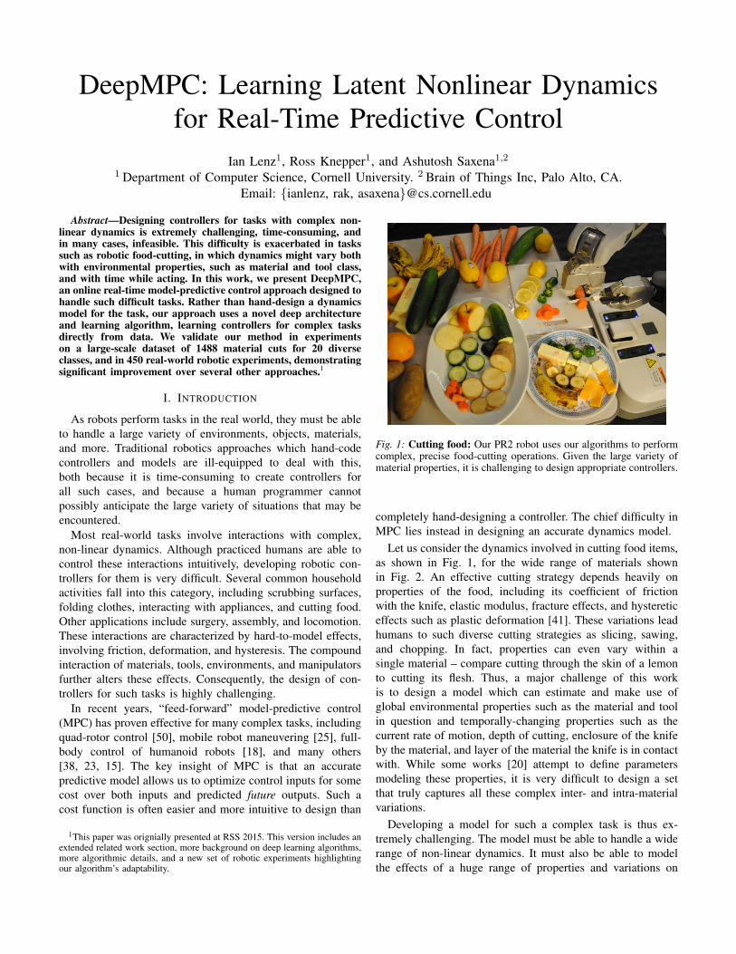
Fig. 3: Variation in cutting dynamics: plots showing desired (green) and actual (blue) trajectories, along with error (red) obtained using astiffness controller while cutting butter (left) and a lemon at low (middle) and high (right) rates of vertical motion. Butter resists the knifesignificantly less than the lemon. Even though only the vertical cutting rate is the only change between the middle and right-hand plots,dynamics along the sawing axis also change significantly. Dynamics also vary with time for the lemon as the knife cuts through the skinand into the flesh.

material types) may not be directly observable. Partially-

Observable MDPs (POMDPs), which have been applied to

such diverse problems as action anticipation for table tennis

[55], robotic grasping [26], navigation [19], avoid these as-

sumptions. However, they typically still make others, such as

locally linear dynamics [9] or discrete action spaces [20]. In

this work, both our states and actions will be continous-valued,

and we will directly model the fact that task dynamics depend

on some unobserved properties.

Feed-forward model-predictive control allows controls to

adapt online by optimizing some cost function over predicted

future states. These approaches have gained increased attention

as modern computing power makes it feasible to perform

optimization in real time. Shim et al. [50] used MPC to

control multiple quad-rotors in simulation, while Howard et al.

[25] performed intricate maneuvers with real-world mobile

robots. Erez et al. [18] used MPC for full-body control of

a humanoid robot. These approaches have been extended to

many other tasks, including underwater vehicle control [38],

visual servoing [23], and even heart surgery [15]. However, all

these works assume the task dynamics model is fully specified.

B. Model Learning for Control

Model learning for robot control has also been a very active

area, and we refer the reader to a review of work in the area by

Nguyen-Tuong and Peters [43]. While early works in model

learning [2, 42] fit parameters of some hand-designed task-

specific model to data, such models can be difficult to design

and may not generalize well to new tasks. Thus, several recent

works attempt to learn more general dynamics models such

as Gaussian mixture models [11, 28] and Gaussian processes

[29]. Neural networks [12, 10] are another common choice

for learning general non-linear dynamics models. The highly

parameterized nature of these models allows them to fit a wide

variety of data well, but also makes them very susceptible to

overfitting.

C. Deep Learning

Modern deep learning methods retain the advantages of

neural networks, while using new algorithms and network

architectures to overcome their drawbacks. Due to their ef-

fectiveness as general non-linear learners [4], deep learning

has been applied to a broad spectrum of problems, including

visual recognition [24, 32], natural language processing [13],

acoustic modeling [40], robotic grasping [33] and many others.

Recurrent deep networks have proven particularly effective

for time-dependent tasks such as text generation [53] and

speech recognition [22]. Factored conditional models using

multiplicative interactions have also been shown to work well

for modeling short-term temporal transformations in images

[39]. More recently Taylor and Hinton [54] applied these

models to human motion, but did not model any control inputs,

and treated the conditioning features as a set of fully-observed

“motion styles”.

A few works have applied deep learning directly to robotic

manipulation. Lenz et al. [33] use a deep network to perform

vision-based grasping of novel objects from RGB-D data.

Sung et al. [51] use deep learning to perform transfer learning

for trajectories for manipulating household appliances. In both

cases, their deep learning methods are limited to determining a

manipulation plan – a grasping pose in the former case, and an

end-effector trajectory in the latter – and then standard motion

control algorithms are used to execute this plan. No deep

networks are used for online control. Levine et al. [35] use a

deep network to learn control policies, and will be discussed

in more detail below.

D. Policy Learning

Several recent approaches to control learning first learn a

dynamics model, then use this model to learn a policy which

maps from system state to control inputs. These works often

iteratively use this policy to collect more data and re-learn

a new policy in an online learning approach. Levine et al.

[35] use a Gaussian mixture model (GMM) where linear

models are fit to each cluster, while Deisenroth and Rasmussen

[14] use a Gaussian process (GP.) Experimentally, both these

models gave less accurate predictions than ours for robotic

food-cutting. The GP also had very long inference times

(roughly 106 times longer than ours) due to the large amount

of training data needed. For details, see Section VIII. This

weak performance is because they use only temporally-local

information, while our model uses learned recurrent features to

integrate long-term information and model unobserved system

properties such as materials.

These works focus on online policy search, while here

we focus on modeling and application to real-time MPC.

Our model could be used along with them in a policy-

learning approach, allowing them to model dynamics with

environmental and temporal variations. However, our model is

efficient enough to optimize for predictive control at run-time.

This avoids the possibility of learned policies overfitting the

training data and allows the cost function and its parameters

to be changed online. It also allows our model to be used with

other algorithms which use its predictions directly.

E. Robotic Manipulation

Luo and Hauser [36] developed a system which adapts

manipulation to unknown system parameters, but requires a

parameterized dynamics model. Koval et al. [30] developed

a new algorithm for planar contact manipulation which de-

composes pre- and post-contact policies. Maitin-Shepard et al.

[37] developed a system for robotic towel-folding. This system

focused on the perception aspects of the problem, and assumes

uniformity and compliance in the material being manipulated.

Several recent works have applied robotic manipulation to

kitchen operations. Bollini et al. [8] developed a vision-based

robotic system for preparing and baking cookies, while Beetz

et al. [3] developed a system for preparing pancakes. Gemici

and Saxena [20] presented a learning system for manipulating

deformable objects which infers a set of material properties,

then uses these properties to map objects to a latent set

of haptic categories which are used to determine how to

manipulate the object. However, their approach requires a

predefined set of properties (plasticity, brittleness, etc.), and

chooses between a small set of discrete actions. By contrast,

our approach performs continuous-space real-time control, and

uses learned latent features to model material properties and

other variations, avoiding the need for hand-design. All three

of these works also apply non-reactive stiffness controllers.

III. PROBLEM DEFINITION AND SYSTEM

In this work, we focus on the task of cutting a wide range of

food items. This problem is a good testbed for our algorithms

because of the variety of dynamics involved in cutting different

materials. Designing individual controllers for each material

would be very time-consuming, and hand-designing accurate

dynamics models for each would be nearly infeasible.

For the task of cutting, we define gripper axes as shown

in Fig. 4, such that the X axis points out of the point of the

knife, Y axis normal to the blade, and Z axis vertically. Here,

we consider linear cutting, where the goal is to make a cut

of some given length along the Z axis. The control inputs

Fig. 4: Gripper axes: PR2’s gripper with knife grasped, showing theaxes used in this paper. The X (“sawing”) axis points along the bladeof the knife, Y points normal to the blade, and Z points vertically.

to the system are denoted as u(t) = (F(t)x , F

(t)y , F

(t)z ), where

F(t)x represents the force, in Newtons, applied along the end-

effector X axis at time t. The physical state of the system is

x(t) = (P(t)x , P

(t)y , P

(t)z ) where P

(t)x is the X coordinate of

the end-effector’s position at time t.

A simple approach to control for this problem might use

a fixed-trajectory stiffness controller, where control inputs are

proportional to the difference between the current state x(t)

and some desired state x∗(t) taken from a given trajectory.

Fig. 3 shows some examples which demonstrate the diffi-

culties inherent in this approach. While some materials, such

as the butter shown on the left, offer very little resistance,

allowing a stiffness controller to accurately follow a given

trajectory, others, such as the lemon shown in the remaining

two plots, offer more resistance, causing significant deviation

from the desired trajectory. When cutting a lemon, we can also

see that the dynamics change with time, resisting the knife

more as it cuts through the skin, then less once it enters the

flesh of the lemon. The dynamics of the sawing and vertical

axes are also coupled - increasing the rate of vertical motion

increases error along the sawing axis, even though the same

controls are used for that axis. This coupled behavior presents

additional challenges for modeling and control, as these axes

must be considered together.

In our approach, we fix the orientation of the end-effector,

as well as the position of the knife along its Y axis, using

stiffness control to stabilize these. However, even though our

primary goal is to move the knife along its Z axis, as shown

in Fig. 3, the X and Z axes are strongly coupled for this

problem. Thus, our algorithm performs control along both the

X and Z axes. This allows “sawing” and “slicing” motions

in which movement along the X axis is used to break static

friction along the Z axis and enable forward progress. We use

a nonlinear function f to predict future states:

x(t+1) = f(x(t), u(t+1)) (1)

We can apply this formula recurrently to predict further into

the future, e.g. x(t+2) = f(x(t+1), u(t+2)). When performing

recurrent prediction as such, an accurate dynamics model is

extremely important as errors will accumulate over multiple

timesteps.

A. Model-Predictive Control: Background

In this work, we use a model-predictive controller to control

the cutting hand. Such controllers have been shown to work

extremely well for a wide variety of tasks for which hand-

defined controllers are either difficult to define or simply

cannot suffice [25, 18, 38, 15]. Defining Xt:k as the system

state from time t through time k, and Ut:k similarly for system

inputs, a model-predictive controller works by finding a set of

optimal inputs U∗

t+1:t+T which minimize some cost function

C(Xt+1:t+T , Ut+1:t+T ) over predicted state X and control

inputs U for some finite time horizon T :

U∗

t+1:t+T = arg maxUt+1:t+T

C(Xt+1:t+T , Ut+1:t+T ) (2)

This approach is powerful, as it allows us to leverage

our knowledge of task dynamics f(x, u) directly, predicting

future interactions and proactively avoiding mistakes rather

than simply reacting to past observations. It is also versatile,

as we have the freedom to design C to define optimality

for some task. The chief difficulty lies in modeling the task

dynamics f(x, u) in a way that is both differentiable and quick

to evaluate, to allow online optimization.

IV. MODELING TIME-VARYING NON-LINEAR DYNAMICS

WITH DEEP NETWORKS

Hand-designing models for the entire range of potential

interactions encountered in complex tasks such as cutting food

would be nearly impossible. Our main challenge in this work

is then to design a model capable of learning non-linear, time-

varying dynamics. This model must be able to respond to

short-term changes, such as breaking static friction, and must

be able to identify and model variations caused by varying

materials and other properties. It must be differentiable with

respect to system inputs, and the system outputs and gradients

must be fast to compute to be useful for real-time control.

We choose to base our model on deep learning algorithms,

a strong choice for our problem for several reasons. They

have been shown to be general non-linear learners [4], but re-

main differentiable using efficent back-propagation algorithms.

When time is an issue, as in our case, network sizes can be

scaled down to trade accuracy for computational performance.

Although deep networks can learn any non-linear function,

care must still be taken to design a task-appropriate model. As

shown in Fig. 7, a simple deep network gives relatively weak

performance for this problem. Thus, one major contribution

of this work is to design a novel deep architecture for mod-

eling dynamics which might vary both with the environment,

material, etc., and with time while acting. In this section, we

describe our architecture, shown in Fig. 5 and motivate our

design decisions in the context of modeling such dynamics.

A. Deep Learning - Background

Before describing our new architecture for handling com-

plex, varying dynamics, we will first describe previous work

which makes up some components of this architecture and

algorithm.

Unsupervised Feature Learning: Unsupervised feature learn-

ing is one of the major strengths of modern deep learning ap-

proaches. Even for unlabled data, these algorithms are capable

of learning useful features which can be used to initialize the

network before supervised learning. Since they are generic

to the type of data used as input, they can be applied to

learned features to learn multiple layers of representation.

Here, we will apply a variant of the sparse auto-encoder (SAE)

algorithm [21], which learns features which reconstruct the

training data well while activating sparsely (e.g. for a given

case, only a few features should have high values.) Initializing

the network in this way helps to avoid overfitting by giving

supervised learning a better, more general starting point.

Back-propagation: During both supervised fine-tuning and

some gradient-based unsupervised learning algorithms such

as SAE, we use back-propagation to efficiently compute cost

function gradients with respect to each parameter of the

network. This works by first performing forward inference

in the network, then computing the cost function and its

gradient with respect to its inputs (from the network.) We can

then iteratively propagate this gradient through the network,

computing the gradient of the cost function with respect to

each hidden unit and weight.

A similar approach can be used to compute cost function

gradients with respect to system inputs during online MPC.

Here, gradients with respect to network parameters are ir-

relevant, so we propagate cost function gradients backwards

through each layer of hidden features until we reach the

system inputs. This lets us quickly and efficiently compute

the gradient of some cost function over network outputs with

respect to system inputs, allowing us to perform real-time

gradient-based optimization for MPC.

Conditional Features: When modeling dynamics which de-

pend on the robot’s environment, we want to be able to condi-

tion the current dynamic response on some set of environmen-

tal properties. Factored conditional nodes [39, 54] are able to

model conditional structures such as this by learning weights

from each set of inputs to some hidden “factors.” Each factor

then multiplies all inputs it recieves, effectively scaling the

contribution of each set of inputs based on features extracted

from the others. When modeling dynamics, this is useful as

it allows different dynamics to be activated or deactivated

depending on environmental properties. Such features have

also been shown to be useful in detecting transformations,

such as shifts and rotations in natural images [39], a behavior

which we will use when modeling time-varying properties.

Temporal Recurrence: When modeling time-dependent be-

havior, it is useful to re-use past information and features.

Temporal recurrence [48] allows us to do so by forming

weights to a set of features from the same features for the

previous timestep, and, in turn, feeding these features forwards

to the next. This allows us to naturally re-use features and

integrate long-term information, while still allowing features

to change over time. This is also memory-efficient, as we need

only remember one additional set of features (the previous

timestep’s) and do not need to record all observed features.

However, recurrent models introduce additional difficulty

during training, in particular in cases such as recurrent dy-

namic prediction where the model outputs are also used

recurrently. If the network is not initialized well, inaccurate

predictions will be fed forwards, causing increased inaccuracy

in future timesteps, leading to the “exploding gradient” prob-

lem when already-huge error gradients are further scaled up

during back-propagation [5]. Such gradients cause problems

for gradient-based learning algorithms and can often lead to

overfitting the training data. Thus, in this work, we present a

new algorithm for training our recurrent model for physical

prediction which iteratively initializes portions of it to avoid

these issues.

B. DeepMPC Architecture

In order to properly model complex dynamics conditioned

on environmental properties which might vary with time, we

now define a new deep architecture. This architecture retains

the strengths of standard deep learning algorithms while giving

superior predictive performance for complex tasks such as

food cutting, as shown in Section VIII.

Dynamic Response Features: When modeling physical dy-

namics, it is important to capture short-term input-output

responses. Thus, rather than learning features separately for

system inputs u and outputs x, the basic input features

used in our model are a concatenation of both. It is also

important to capture high-order and delayed-response modes

of interaction. Thus, rather than considering only a single

timestep, we consider blocks thereof when computing these

features, so that for block b, with block size B, we have visible

input features v(b) = (Xb∗B:(b+1)∗B−1, Ub∗B:(b+1)∗B−1). For

known timesteps, we use the observed values of x, while for

future timesteps, we use x as predicted by our model. For

more details on our feature pre-processing, see Section VI.

Conditional Dynamic Responses: For tasks such as material

cutting, local dynamics might be conditioned on both time-

invariant and time-varying properties. Thus, we must design

a model which operates conditional on past information. We

do so by introducting factored conditional units [39], where

features from some number of inputs modulate multiplicatively

and are then weighted to form network outputs. Intuitively,

this allows us to blend a set of models based on features

extracted from past information. Since our model needs to

incorporate both short- and long-term information, we allow

three sets of features to interact – the current control inputs, the

past block’s dynamic response, and latent features modeling

long-term observations, described below. Although the past

block’s response is also included when forming latent features,

including it directly in this conditional model frees our latent

features from having to model such short-term dependencies.

We use c to denote the current timeblock, f to denote the

immediate future one, l for latent features, and o for outputs.

Take Nv as the number of features v, Nx as the number of

states x, and Nu as the number of inputs u in a block, and

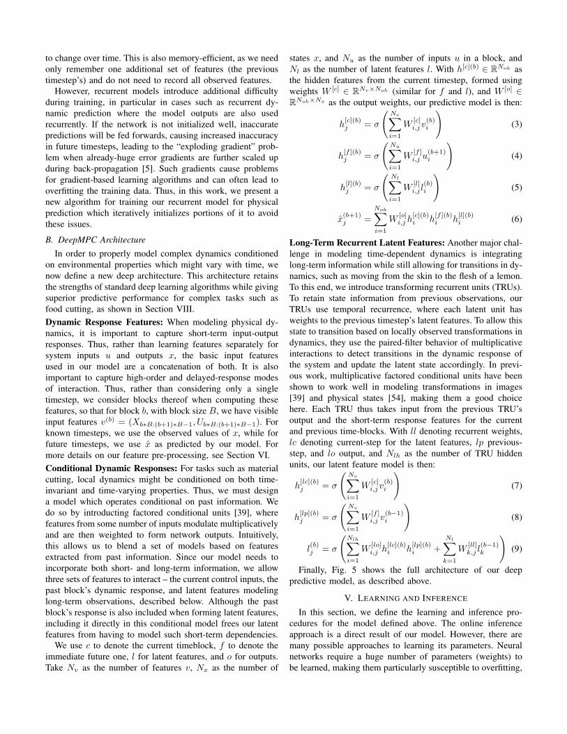
Nl as the number of latent features l. With h[c](b) ∈ RNoh as

the hidden features from the current timestep, formed using

weights W [c] ∈ RNv×Noh (similar for f and l), and W [o] ∈

RNoh×Nx as the output weights, our predictive model is then:

h[c](b)j = σ

(

Nv∑

i=1

W[c]i,j v

(b)i

)

(3)

h[f ](b)j = σ

(

Nu∑

i=1

W[f ]i,j u

(b+1)i

)

(4)

h[l](b)j = σ

(

Nl∑

i=1

W[l]i,j l

(b)i

)

(5)

x(b+1)j =

Noh∑

i=1

W[o]i,j h

[c](b)i h

[f ](b)i h

[l](b)i (6)

Long-Term Recurrent Latent Features: Another major chal-

lenge in modeling time-dependent dynamics is integrating

long-term information while still allowing for transitions in dy-

namics, such as moving from the skin to the flesh of a lemon.

To this end, we introduce transforming recurrent units (TRUs).

To retain state information from previous observations, our

TRUs use temporal recurrence, where each latent unit has

weights to the previous timestep’s latent features. To allow this

state to transition based on locally observed transformations in

dynamics, they use the paired-filter behavior of multiplicative

interactions to detect transitions in the dynamic response of

the system and update the latent state accordingly. In previ-

ous work, multiplicative factored conditional units have been

shown to work well in modeling transformations in images

[39] and physical states [54], making them a good choice

here. Each TRU thus takes input from the previous TRU’s

output and the short-term response features for the current

and previous time-blocks. With ll denoting recurrent weights,

lc denoting current-step for the latent features, lp previous-

step, and lo output, and Nlh as the number of TRU hidden

units, our latent feature model is then:

h[lc](b)j = σ

(

Nv∑

i=1

W[c]i,j v

(b)i

)

(7)

h[lp](b)j = σ

(

Nv∑

i=1

W[f ]i,j v

(b−1)i

)

(8)

l(b)j = σ

(

Nlh∑

i=1

W[lo]i,j h

[lc](b)i h

[lp](b)i +

Nl∑

k=1

W[ll]k,j l

(b−1)k

)

(9)

Finally, Fig. 5 shows the full architecture of our deep

predictive model, as described above.

V. LEARNING AND INFERENCE

In this section, we define the learning and inference pro-

cedures for the model defined above. The online inference

approach is a direct result of our model. However, there are

many possible approaches to learning its parameters. Neural

networks require a huge number of parameters (weights) to

be learned, making them particularly susceptible to overfitting,

h[lc]h[lp]

l(b−1) l(b)

h[l]

h[c]

h[f ]

x(b+1)

v(b−1) v(b) u(b+1)

Fig. 5: Deep predictive model: Architecture of our recurrent conditional deep predictive dynamics model. Transforming recurrent units(TRUs) on the left model time-varying latent properties which affect system dynamics. On the right, conditional multiplicative modulationis used again to condition future system responses on past observed dynamics and latent features.

and recurrent networks often suffer from instability in future

predictions, causing large gradients which make optimization

difficult (the “exploding gradient” problem [5]).

To avoid these issues, we define a new three-stage learning

approach which pre-trains the network weights before using

them for recurrent modeling. Deep learning methods are non-

convex, and converge to only a local optimum, making our

approach important in ensuring that a good optimum which

does not overfit the training data is reached.

Inference: During inference for MPC, we are currently at

some time-block b with latent state l(b), known system state

x(b) and control inputs u(b). Future control inputs Ut+1:t+T

are also given, and our goal is then to predict the future system

states Xt+1:t+T up to time-horizon T , along with the gradients

∂X/∂U for all pairs of x and u. These gradients will then be

used by MPC to optimize the control inputs u.

We perform this inference by applying our model recur-

rently to predict future states up to time-horizon T , using pre-

dicted states x and latent features l as inputs to our predictive

model for subsequent timesteps, e.g. when predicting x(b+2),

we use the known x(b) along with the predicted x(b+1) and

l(b+1) as inputs.

Our model’s outputs (x) are differentiable with respect to all

its inputs, allowing us to take gradients ∂X/∂U using an ap-

proach similar to the backpropagation-through-time algorithm

used to optimize model parameters during learning, as shown

in Algorithm 1. We can in turn use these gradients with any

gradient-based optimization algorithm to optimize Ut+1:t+T

with respect to some differentiable cost function C(X,U). No

online optimization is necessary to perform inference for our

model. For details on our online optimization approach, see

Section VII.

Learning: During learning, our objective is to use

our training data to learn a set of model parame-

ters Θ = (W [f ],W [c],W [l],W [o],W [lp],W [lc],W [ll],W [lo])which minimize prediction error while avoiding overfitting.

A naive approach to learning might randomly initialize Θ,

then optimize the entire recurrent model for prediction error.

However, random weights would likely cause the model to

make inaccurate predictions, which will in turn be fed forwards

to future timesteps. This could cause huge errors at time-

horizon T , which will in turn cause large gradients to be back-

propagated, resulting in instability in the learning and overfit-

ting to the training data. To remedy this, we propose a multi-

stage pre-training approach which first optimizes some subsets

of the weights, leading to much more accurate predictions and

less instability when optimizing the final recurrent network.

We show in Fig. 7 that our learning algorithm significantly

outperforms random initialization.

Phase 1: Unsupervised Pre-Training: In order to obtain

a good initial set of features for l, we apply an unsupervised

learning algorithm similar to the sparse auto-encoder algorithm

[21] to train the non-recurrent parameters of the TRUs. This

algorithm first projects from the TRU inputs up to l, then

uses the projected l to reconstruct these inputs. The TRU

weights are optimized for a combination of reconstruction

error and sparsity in the outputs of l. Taking vm,k as the

visible features for the kth time-block of training case m,

M as the number of training cases, and Tm as the number of

timesteps for case m, and g(l) as some function penalizing

latent feature activation to induce sparsity, our unsupervised

pre-training phase proceeds as:

Θ∗ = arg minΘ

M∑

m=1

Tm/B∑

b=2

||v(m,b−1) − v(m,b−1)||22

+ ||v(m,b) − v(m,b)||22 + λ

K∑

j=1

g(l(b)j )

(10)

h[ll](b)j =

Nl∑

a=1

W[ll]j,a l

(b)a (11)

v(b−1)i =

Nlh∑

j=1

W[lp]i,j h

[ll](b)j h

[lc](b)j (12)

v(t)i =

Nlh∑

j=1

W[lp]i,j h

[ll](b)j h

[lp](b)j (13)

Phase 2: Short-term Prediction Training: While we could

now use these parameters as a starting point to optimize a

fully recurrent multi-step prediction system, we found that in

practice, this lead to instability in the predicted values, since

inaccuracies in initial predictions might “blow up” and cause

huge deviations in future timesteps.

Instead, we include a second pre-training phase, where we

train the model to predict a single timestep into the future. This

allows the model to adjust from the task of reconstruction to

that of physical prediction, without risking the aforementioned

instability. For this stage, we remove the recurrent weights

from the TRUs, effectively setting all W [ll] to zero and

ignoring them for this phase of optimization.

Taking x(m,k) as the state for the kth time-block of training

case m, M as the number of training cases, and Bm as the

number of timeblocks for case m, this stage optimizes:

Θ∗ = arg minΘ

M∑

m=1

Bm−1∑

b=2

||x(m,b+1) − x(m,b+1)||22 (14)

Phase 3: Warm-Latent Recurrent Training: Once Θ has

been pre-trained by these two phases, we use them to initialize

a recurrent prediction system which performs inference as

described above. We then optimize this system to minimize the

sum-squared prediction error up to T timesteps in the future,

using a variant of the backpropagation-through-time algorithm

commonly used for recurrent neural networks [48].

When run online, our model will typically have some

amount of past information, as we allow a short period where

we optimize forces while a stiffness controller makes an

initial inwards motion. Thus, simply initializing the latent

state “cold” from some intial state and immediately penalizing

prediction error does not match well with the actual use of the

network, and might in fact introduce overfitting by forcing the

model to rely more heavily on short-term information. Instead,

we train our model for a “warm” start. For some number of

initial time-blocks Bw, we propagate latent state l, but do not

predict or penalize system state x, only doing so after this

warm-up phase. We still back-propagate errors from future

timesteps through the warm-up latent states as normal.

Algorithm 1 Recurrent Prediction and Cost Gradients for

MPC

Input:

Previous and current dynamic responses v(b−1), v(b)

Current latent state l(b)

Future control inputs Ut+1:t+T

Output:

Predicted future state Xt+1:b+T

Cost function value C(Xt+1:t+T , Ut+1:t+T )Cost gradients ∂C(Xt+1:t+T , Ut+1:t+T )/∂Ut+1:t+T

Define C(x(i), U) as the direct contribution of x(i) to

C(Xt+1:t+T , Ut+1:t+T ) (ignoring recurrent effects.)

Define C(U) as the direct contribution of U to the cost

function (e.g. via smoothing/regularization terms)

Forward prediction:

for k = 1:T/BCompute l(b+k) from eq. (9)

Compute x(b+k) from eq. (6)

end

Compute C(Xt+1:t+T , Ut+1:t+T )

Back-propagating gradients:

dXBack1 = 0; dXBack2 = 0;

dUBack1 = 0; dUBack2 = 0;

dLBack1 = 0;

for k = T/B:1

Compute current cost function gradient, back-prop to udXCur = ∂C(x(b+k), U)/∂x(b+k)

dXCur = dXCur + dXBack1;

∂C(X, U)/∂u(b+k) = dXCur * ∂x(b+k)/∂u(b+k)

+ ∂C(U)/∂u(b+k) + dUBack1

Back-propagate gradients to previous timesteps

dXBack1 = dXBack2 + dXCur * ∂x(b+k)/∂x(b+k−1)

+ dLBack1 * ∂l(b+k)/∂x(b+k−1)

dUBack1 = dUBack2 + dXCur * ∂x(b+k)/∂u(b+k−1)

+ dLBack1 * ∂l(b+k)/∂u(b+k−1)

dXBack2 = dXCur * ∂x(b+k)/∂x(b+k−2)

+ dLBack1 * ∂l(b+k)/∂x(b+k−2)

dUBack2 = dXCur * ∂x(b+k)/∂u(b+k−2)

+ dLBack1 * ∂l(b+k)/∂u(b+k−2)

dLBack1 = dLBack1 * ∂l(b+k)/∂l(b+k−1)

+ dXCur * ∂x(b+k)/∂l(b+k−1)

end

VI. SYSTEM DETAILS

Learning System: We used the L-BFGS algorithm, shown to

give strong results for deep learning methods [31], to optimize

our model during learning. While larger network sizes gave

slightly (∼10%) less error, we found that setting Nlh = 50,

Nl = 50, and Noh = 100 was a good tradeoff between accuracy

and computational performance. We found that block size B= 10, giving blocks of 0.1s, gave the best performance. When

implemented on the GPU in MATLAB, all phases of our

learning algorithm took roughly 30 minutes to optimize.

MPC Cost Function: In order to perform MPC, we need to

define a cost function C(X,U) for our task. For food cutting,

we design a cost function with two main components, with βdefining the weighting between them:

C(X,U) = Ccut(X) + βCsaw(X) (15)

The first, Ccut, drives the controller to move the knife down-

wards. It penalizes the height of the knife at each timestep,

with an additional penalty at the final timestep allowing a

tradeoff between immediate and eventual downwards motion:

Ccut(X) =

t+T∑

k=t

P (k)z + γP (t+T )

z (16)

The second term, Csaw, keeps the tip of the knife inside some

reasonable “sawing range” along the X axis, ensuring that it

actually cuts through the food. Since any valid position is

acceptable, this term will be zero inside some margins from

this range, then become quadratic once it passes those margins.

Taking P ∗

x as the center point of the sawing range, ds as the

range, and λ as the margin, we define this term as:

Csaw(X) =t+T∑

k=t

(

max{

0, |P (k)x − P ∗

x | − ds + λ})2

(17)

We also include terms performing first- and second-order

smoothing and L2 regularization on the control forces.

Data Pre-Processing: In order to allow our learning algo-

rithm to learn a better model for our data, we perform light

pre-processing. We represent position features for each block

relative to the last position in the previous block – e.g. if the

previous block ended with an X-position of 0.4 m and the

current block started with an X-position of 0.5 m, the first

X-position feature for the current block would be 0.1 m. This

representation avoids overfitting to absolute positions, while

still representing relative motions and allowing us to easily

reconstruct an absolute-position trajectory. Since we want to

capture absolute, not relative, input forces, we do not offset

them in this way.

The only whitening we perform on these features is to scale

them so all features for a particular channel (e.g. X-positions,

Z-forces, etc.) have unit standard deviation. We scale per-

channel – applying the same scaling to all B features for a

particular channel – rather than per-feature in order to preserve

relative values within a channel. For similar reasons, we do

not shift values e.g. to set the mean to zero as is common in

other whitening approaches.

One advantage to our whitening approach is that it allows

us to transfer this scaling to the input-layer weights during

inference. For example, if we applied a scaling factor of 0.1

to X-position inputs during learning, we can simply scale the

weights to the X-position used during inference by 0.1 and

use un-whitened X-position values (still offset as above.) This

saves computation time by avoiding performing scaling on new

input features.

Fig. 6: Online system: Block diagram of our DeepMPC system.Parameters learned using our three-stage deep learning algorithm areloaded by the optimization process, which then continually predictsfuture states and updates future controls based on these predictions.The control process takes state information from the robot, transmitsit to the optimization process, and transmits controls optimized bythat process to the robot.

VII. REAL-TIME ROBOTIC DEEPMPC SYSTEM

Robotic Platform: For both data collection and online evalua-

tion of our algorithms, we used a PR2 robot. The PR2 has two

7-DoF manipulators with parallel-plate grippers, and a reach

of roughly 1m. For safety reasons, we limit the forces applied

by PR2’s arms to 30N along each axis, which was sufficient

to cut every material tested. PR2 natively runs the Robot

Operating System (ROS) [47]. Its arm controllers recieve robot

state information in the form of joint angles and must publish

desired motor torques at a hard real-time rate of 1KHz.

Online Model-Predictive Control System: The main chal-

lenge in designing a real-time model-predictive controller for

this architecture lies in allowing prediction and optimization

to run continuously to ensure optimality of controls, while

providing the model with the most recent state information

and performing control at the required real-time rate. As

shown in Fig. 6, we solve this by separating our online

system into two processes (ROS nodes), one performing

continuous optimization, and the other real-time control. These

processes use a shared memory space for high-rate inter-

process communication. This approach is modular and flexible

- the optimization process is generic to the robot involved

(given an appropriate model), while the control process is

robot-specific, but generic to the task at hand. In fact, models

for the optimization process do not even need to be learned

locally, but could be shared using an online platform [49].

The control process is designed to perform minimal com-

putation so that it can be called at a rate of 1KHz. It

recieves robot state information in the form of joint angles,

and control information from the optimization process as end-

effector forces. It performs forward kinematics to determine

end-effector pose, transmits it to the optimization process, and

uses it to determine restoring forces for axes not controlled by

MPC. It translates the combination of these forces and those

recieved from MPC to a set of joint torques sent to the arm.

All operations performed by the control process are at most

quadratic in terms of the number of degrees of freedom of the

arm, allowing each call to run in roughly 0.1 ms on PR2.

The optimization process runs as a continuous loop. When

started, it loads model parameters (network weights) from

disk. Cost function parameters are loaded from a ROS pa-

rameter server, allowing them to be changed online. The

optimization loop first uses past robot states (received from

the control process) and control inputs along with past latent

state and the future forces being optimized to predict future

state using our model. It then uses this state to compute

the gradients of the MPC cost function and back-propagates

these through our model, yielding gradients with respect to

the future forces. It optimizes these forces using a variant of

the AdaGrad algorithm [16], a form of gradient descent in

which gradient contributions are scaled by the L2 norm of past

gradients, chosen because it is efficient in terms of function

evaluations while avoiding scaling issues. This process is

implemented using the Eigen matrix library [17], allowing the

optimization loop to run at a rate of over 1.2kHz.

VIII. PREDICTION EXPERIMENTS

In order to evaluate our model learning approach as com-

pared to other state-of-the-art methods, we performed experi-

ments evaluating prediction accuracy on our extensive dataset

of 1488 material cuts. In the next section, we will also evaluate

our algorithms on a real-world PR2 robot.

Dataset: Our material interaction dataset contains 1488 exam-

ples of robotic food-cutting for 20 different materials (Fig. 2).

We collected data from three different settings. First, a fixed-

parameter setting in which trajectories as shown in the leftmost

two columns of Fig. 3 were used with a stiffness controller.

Second, for 8 of the 20 materials in question, data was

collected while a human tuned a stiffness controller to improve

cutting rate. This data was not collected for all materials to

avoid giving the learning algorithm and controller near-optimal

cases for all materials. Third, a randomized setting where most

parameters of the controller, including cutting and sawing rate

and stiffnesses, but excluding sawing range (still fixed at 4cm)

were randomized for each stroke of the knife. This helped to

obtain data spanning the entire range of possible interactions.

Setting: In order to test our model, we examine its predictive

accuracy compared to several other approaches. Each model

was given 0.7s worth of past trajectory information (forces

and known poses) and 0.5s of future forces and then asked to

predict the future end-effector trajectory. For this experiment,

we used 70% of our data for training, 10% for validation, and

20% for testing, sampling to keep each set class-balanced.

Baselines: For prediction, we include a linear state-space

model, an ARMAX model which also weights a range of past

0 0.05 0.1 0.15 0.2 0.25 0.3 0.35 0.4 0.45 0.50

2

4

6

8

10

12

Time (s)

Me

an

L2

err

or

(mm

)

Linear SS

GMM−Linear

ARMAX

Simple Deep

5−NN

Ours, Non−Recur.

Gaussian Process

Recur. Deep

Ours, Rand. Init

Ours

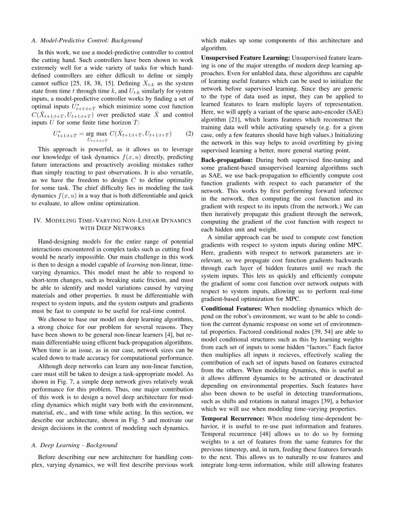
Fig. 7: Prediction error: Mean L2 distance (in mm) from predictedto ground-truth trajectory from 0.01s to 0.5s in the future. Whilemost models give similar performance up to 0.1s, models withlinear components give very weak long-term results. Non-parametricmethods give better results, but are hampered by expensive inferencewhich scales poorly. Recurrent deep networks give the best results,with our approach outperforming all others after 0.1s, reducing errorat 0.5s by 46% as compared to the baseline recurrent network

TABLE I: Confidence at 0.5s: Mean L2 error and 95% confidenceinterval at prediction time of 0.5s (all in mm)

Algorithm Mean95% Conf.

Min. Max.

Linear SS 11.46 0.89 38.58GMM-Linear 8.96 0.58 31.80ARMAX 8.66 0.79 31.36Simple Deep 4.90 0.52 18.315-NN 4.25 0.22 19.24Ours, Non-Recur. 3.80 0.35 15.03Gaussian Process 3.56 0.27 14.85Recur. Deep 3.27 0.47 12.14Ours, Rand. Init 2.78 0.33 10.41Ours 1.78 0.16 7.55

states, and a K-Nearest Neighbors (K-NN) model (5-NN gave

the best results) as baseline algorithms. We also include a

GMM-linear model [34], and a Gaussian process (GP) model

[14], trained using the GPML package [45]. Additionally, we

compare to standard recurrent and non-recurrent two-layer

deep networks, and versions of our approach without recur-

rence and without pre-training (randomly initializing weights,

then training for recurrent prediction).

Results: Fig. 7 shows performance for each model as mean

L2 distance from predicted to ground truth trajectory vs.

prediction time in the future. Temporally-local (piecewise-)

linear methods (linear SS, GMM-linear, and ARMAX) gave

weak performance for this problem, each yielding an average

error of over 8mm at 0.5s. This shows, as expected, that linear

models are a poor fit for our highly non-linear problem.

Instance-based learning methods – K-NN and Gaussian pro-

cesses – gave better performance, at an average of 4.25mm and

3.56mm, respectively. Both outperformed the baseline two-

layer non-recurrent deep network, which gave 4.90mm error.

The GP gave the best performance of any temporally-local

model, although this came at the cost of extreme inference

time, taking an average of 3361s (56 minutes) to predict 0.5s

into the future, 1.18x106 times slower than our algorithm,

whose MATLAB implementation took only 3.1ms.

The relatively unimpressive performance of a standard two-

layer deep network for this problem underscores the need

for task-appropriate architectures and learning algorithms. In-

cluding conditional structures, as in the non-recurrent version

of our model and temporal recurrence reduced this error

to 3.80mm and 3.27mm, respectively. Even when randomly

initialized, our model outperformed the baseline recurrent

network, giving only 2.78mm error, showing the importance of

using an appropriate architecture. Using our learning algorithm

further reduced error to 1.78mm, 36% less than the randomly-

initialized version and 46% less than the baseline recurrent

model, demonstrating the need for careful pre-training.

For online model-predictive control, particularly when deal-

ing with real-world variety, worst-case performance is very

important, since we need to ensure that our model will

perform well under any conditions. As shown in Table I,

our approach also gave a tighter and lower 95% confidence

interval of prediction error, from 0.16-7.55mm at 0.5s, a width

of 7.39mm, compared to the baseline recurrent net’s interval

of 0.47-12.14mm, a width of 11.67mm, and the GP’s interval

of 0.27-14.85mm, a width of 14.58mm. In fact, our method

was the only approach whose entire 95% confidence interval

lay under 1cm of error.

IX. ROBOTIC EXPERIMENTS

To evaluate our algorithm’s performance for real-world

robotic control, we performed an extensive series of over 450

experiments on our PR2 robot using the system described in

Sec. VII.

Setting: In these experiments, the robot’s goal was to make

a linear cut between two given points. We selected a subset

of 10 of the 20 materials in our dataset for these experiments,

aiming to span the range of variation in material properties. We

evaluated these experiments in terms of cutting rate, i.e. the

vertical distance traveled by the knife divided by time taken.

Baselines: For control, we validate our algorithm against

several other control methods with varying levels of class

information. First, we compare to a class-generic stiffness

controller, using the same controller for all classes. This

controller was tuned to give a good (>90%) rate of success

for all classes, meaning that it is much slower than necessary

for easy-to-cut classes such as tofu. We also validate against

controllers tuned separately for each of the test classes, using

the same criteria as above, showing the maximum cutting rate

that can be expected from fixed-trajectory stiffness control.

As a middleground, we compare to an algorithm similar to

that of Gemici and Saxena [20], where a set of class-specific

material properties are mapped to learned haptic categories.

We found that learning five such categories assigned all data

for each class to exactly one cluster, and thus used the same

controller for all classes assigned to each cluster. In cases

where this controller was the same as used for the class-tuned

case, we used the same results for both.

Results: Figure 8 shows the results of our series of over 450

robotic experiments. For all materials except butter and tofu,

a paired t-test showed that our DeepMPC controller made a

statistically significant improvement in cutting rate with 95%

confidence. This makes sense as butter and tofu are relatively

soft and easy-to-cut materials. However, for the four materials

for which stiffness control gave the weakest results – lemons,

potatoes, carrots, and apples – our algorithm more than tripled

the mean cutting rate, from 1.5 cm/s to 5.1 cm/s.

One major advantage our approach has over the others

tested is that it treats material properties and classes as latent

and continuous-valued, rather than supervised and discrete.

For intra-class variations which affect dynamics, such as

different varieties of apples or cheeses, different radii of

carrots or potatoes, or varying material temperature, even the

class-specific stiffness controllers were typically limited by

the hardest-to-cut variation. However, our approach’s latent

material properties allowed it to adapt to these, significantly

increasing cutting rates. This was particularly evident for

carrots, whose thickness causes huge variations in dynamics.

While all approaches were tested on both thick and thin

sections of carrot, only ours was able to properly adapt, slicing

easily through thin sections and more carefully through thicker

ones, increasing mean cutting rate from 0.4 cm/s to 4.7 cm/s.

Similar results were observed for potatoes, increasing mean

rate from 3.1 cm/s to 6.8 cm/s.

Another advantage of our approach is its ability to respond

to time-dependent changes in dynamics, thanks to the time-

varying nature of our latent features and the online adaptation

performed by MPC. Such changes occur to some degree as

the knife enters and becomes enclosed by most materials,

particularly in irregular shapes such as potatoes where the

degree of enclosure varies throughout the cut. They are even

more apparent in non-uniform materials, such as lemons, with

variation between the skin and flesh, and apples, which are

much denser and harder to cut closer to the core. Again,

stiffness control was limited by the toughest of these dynamics,

while our approach was able to adapt, typically performing

more sawing for more difficult regions, and quickly moving

downwards for easier ones. This allowed our controller to

increase the mean cutting rate for lemons from 1.3 cm/s to

4.5 cm/s, and for apples from 1.4 cm/s to 4.6 cm/s.

Optimizing its trajectory online also enabled our DeepMPC

controller to exhibit a much more diverse range of behaviors.

Most tuned stiffness controllers were forced to make use of

high-amplitude sawing to ensure continuous motion. How-

ever, our controller was able to use more aggressive cutting

strategies, typically executing smooth slicing motions until it

found its progress impeded. It then used a variety of tech-

niques to break static friction and continue motion, including

high-amplitude sawing, low-amplitude “wiggle” motions, and

reducing and re-applying vertical pressure, even to the point of

picking up the knife slightly in some cases. The latter behavior,

0

5

10

15

20

25

Cu

ttin

g r

ate

(cm

/s)

Stiff., class−general

Stiff., clustered (Gemici)

Stiff., class−specific

Ours

Fig. 8: Robotic experiment results: Mean cutting rates, with bars showing normalized standard deviation, for ten diverse materials.Red bar uses the same controller for all materials, blue bar uses the same for each cluster given by [20], purple uses a tuned stiffnesscontroller for each, and green is our online MPC method. Our algorithm consistently gives higher mean rates, making statistically significantimprovements for all materials except butter and tofu. Particularly significant improvements are seen for tough, varying materials such ascarrots and potatoes.

Fig. 9: Cutting food: Time-series of our PR2 robot using our DeepMPC controller to cut several of the food items in our dataset. Ouralgorithm is able to adapt its strategy for different materials. Note in particular that it picks up the knife slightly, then chops back down whencutting the carrot, and uses more “sawing” motion on tougher materials. Video of these experiments is available at http://deepmpc.cs.cornell.edu

in particular, underscores the strength of predictive control, as

it trades off short-term losses for long-term gains. Stiffness

controllers sometimes became stuck in tough materials such

as thick potatoes and carrots and the cores of apples, and

remained so because downwards force grew as vertical error

increased. Our controller, however, was able to detect and

break such cases using these techniques.

Some examples of the diverse behaviors of our DeepMPC

controller can be seen in Fig. 9 and in the video at http:

//deepmpc.cs.cornell.edu.

A. Handling Variety

In addition to our main experiments, presented above,

we performed a series of additional experiments to test the

adaptive abilities of our controller. For both these experiments,

we chose to use potatoes, as they represent a challenging,

dense material which responds in interesting ways to changes

in temperature and tools (as detailed below.)

Varying Temperature: While the temperature of a material

is not detectable by most robotic platforms (with some notable

exceptions [7]), it can have a huge effect on the cutting dy-

Fig. 10: Different tools: Different knives used to test our algorithm.From left to right, the paring knife used to collect data and train thealgorithm, a shorter, sharper paring knife, a long kitchen knife, awedge-shaped chef’s knife, and a serrated steak knife. In all casesexcept the serrated knife, our algorithm, trained only with the paringknife on the left, was able to maintain comparable cutting rates.

namics of that material. We performed a series of experiments

to validate the robustness of our algorithm to this variation.

For these experiments, we prepared several “cold” potatoes by

placing them in a freezer for 30 minutes, and several “warm”

potatoes by microwaving them for five minutes. Both of these

operations significantly altered the texture of the potato.

We did not tune or alter any controllers to reflect these

new cases. As a baseline, we compare to the class-specific

stiffness controller tuned for potatoes described above. For

our approach, we used the same learned controller as used in

all other robotic experiments, which has no experience with

either warm or cold potatoes, only room-temperature. These

are the same controllers presented as the purple and green

bars, respectively, in Fig. 8, which gave cutting rates of 3.1

cm/s and 6.8 cm/s for room temperature potatoes.

The warm potatoes were much softer and easier to cut than

at room temperature. This allowed the stiffness controller to

track its input trajectory almost exactly, increasing cutting

rate slightly to 3.5 cm/s. Our approach, however, was able

to properly adapt to these new conditions, almost doubling its

cutting rate to 12.0 cm/s.

The cold potatoes were significantly more difficult to cut.

In over half of our trials with cold potatoes, the baseline con-

troller became stuck, with downwards progress halting after

some point. For purposes of rate computation, we considered

the controller to still be cutting until it reached the end of its

input trajectory, leading to an average cutting rate of only 1.8

cm/s. Our controller, once again, was able to properly adapt

to this new case. While its forward progress was sometimes

temporarily halted, it was able to perform motions to break

out and continue cutting, allowing it to achieve a rate of 3.4

cm/s, almost double that of the baseline stiffness controller.

Varying Tools: We also tested our controller, learned using the

paring knife shown in Fig. 4, with a series of other knives, as

shown in Fig. 10. These included a much sharper and slightly

shorter paring knife, a longer kitchen knife, a wedge-shaped

chef’s knife, and a serrated steak knife. Our controller was able

to adapt to the first three knives, giving cutting rates similar to

the results in Fig. 8. The sharp paring knife increased the rate

slightly, to 7.8 cm/s, while the long and wedge knives both lead

to slightly decreased rates of 5.5 and 5.6 cm/s, respectively.

This makes sense, as the sharp paring knife was very similar

to the training knife, only sharper, wheras the long and wedge-

shaped knives were significantly different, leading to different

cutting dynamics, particularly in the case of the wedge-shaped

knife. It is notable that our algorithm experienced only a slight

(roughly 17%) decrease in performance for such a significant

change in tools.

Our algorithm, trained using a straight-edged paring knife,

was not able to use the serrated steak knife to cut a potato.

This makes sense for two reasons:

First, a serrated knife is not, in general, a good tool for

cutting dense vegetables like potatoes. Typically, such knives

are only used for meat, where the main mode of cutting

is splitting muscle fibers, or soft, skinned vegetables such

as tomatoes, where the serration helps to cut through the

skin without smashing the vegetable, which offers minimal

resistance. For dense vegetables, a sharp, straight edge is

necessary to split the vegetable, and even a skilled human

user would have a hard time using a serrated knife.

Second, the dynamics of cutting using a serrated knife are

very different – while a straight-edged knife acts primarily by

splitting the vegetable apart, a serrated knife acts by “eroding”

the food item with its serrations. Food will respond very

differently to the same motion executed by a serrated knife,

so such a knife requires a significantly different dynamics

model and cutting strategy. In particular, straight downwards

motions are ineffective, requiring instead more “sawing” and

less downwards force to allow the serrations to act. Thus,

experience with a straight-edge knife should not be expected

to transfer to a serrated one. However, given new training data,

our algorithm could also learn to use such a knife.

In both these experiments, our algorithm was able to suc-

cessfully handle variations that it was not explicitly trained

for. While varying temperature and tools both significantly

alter cutting dynamics, in all cases but the serrated knife, our

algorithm was able to adapt to these and maintain comparable

cutting rates, even improving them in some cases.

X. CONCLUSION

In this work, we presented DeepMPC, a novel approach

to model-predictive control for complex non-linear dynam-

ics which might vary both with environment properties and

with time while acting. Instead of hand-designing predictive

dynamics models, which is extremely difficult and time-

consuming for such tasks, our approach uses a new deep

architecture and learning algorithm to accurately model even

such complicated dynamics. In experiments on our large-

scale dataset of 1488 material cuts over 20 diverse materials,

we showed that our approach improves accuracy by 46% as

compared to a standard recurrent deep network. In a series of

over 450 real-world robotic experiments for the challenging

problem of robotic food-cutting, we showed that our algorithm

produced significant improvements in cutting rate for all but

the easiest-to-cut materials, and over tripled average cutting

rates for the most difficult ones.

Here, we presented a system which displays adaptability

while learning a good latent representation for complex tasks.

While food-cutting and many other manipulation tasks lend

themselves well to intuitive cost functions, for others we

could envision also learning the cost function used for MPC

from data. In future work, this system could also be extended

to handle multimodal information, e.g. incorporating haptic,

visual, audio, or other data to enhance manipulation. While it

would be extremely difficult to design features which properly

integrate all this information, deep learning allows us to learn

these features directly from data, and our system would allow

us to integrate them into real-time model-predictive control.

ACKNOWLEDGEMENTS

This work was supported in part by Army Research Office

(ARO) award W911NF-12-1-0267, NSF National Robotics

Initiative (NRI) award IIS-1426744, and also by Microsoft

Faculty Fellowship and NSF CAREER Award to Saxena.

REFERENCES

[1] P. Abbeel, A. Coates, M. Quigley, and A. Y. Ng. An ap-

plication of reinforcement learning to aerobatic helicopter

flight. In NIPS, 2007.

[2] C. G. Atkeson, C. H. An, and J. M. Hollerbach. Estimation

of inertial parameters of manipulator loads and links. Int.

J. Rob. Res., 5(3):101–119, Sept. 1986.

[3] M. Beetz, U. Klank, I. Kresse, A. Maldonado,

L. Mosenlechner, D. Pangercic, T. Ruhr, and M. Tenorth.

Robotic Roommates Making Pancakes. In Humanoids,

2011.

[4] Y. Bengio. Learning deep architectures for AI. FTML, 2

(1):1–127, 2009.

[5] Y. Bengio, P. Simard, and P. Frasconi. Learning long-

term dependencies with gradient descent is difficult. IEEE

Transactions on Neural Networks, 5(2):157–166, 1994.

[6] S. Bennett. A brief history of automatic control. Control

Systems, IEEE, 16(3):17–25, Jun 1996. ISSN 1066-033X.

[7] T. Bhattacharjee, J. Wade, and C. C. Kemp. Material

recognition from heat transfer given varying initial con-

ditions and short-duration contact. In RSS, 2015.

[8] M. Bollini, J. Barry, and D. Rus. Bakebot: Baking cookies

with the pr2. In IROS PR2 Workshop, 2011.

[9] E. Brunskill, L. Kaelbling, T. Lozano-Perez, and N. Roy.

Continuous-state POMDPs with hybrid dynamics. In

ISAIM, 2008.

[10] M. V. Butz, O. Herbort, and J. Hoffmann. Exploiting re-

dundancy for flexible behavior: Unsupervised learning in a

modular sensorimotor control architecture. Psychological

Review, 114:1015–1046, 2007.

[11] S. Chernova and M. Veloso. Confidence-based policy

learning from demonstration using gaussian mixture mod-

els. In AAMAS, 2007.

[12] C.-M. Chow, A. G. Kuznetsov, and D. W. Clarke. Succes-

sive one-step-ahead predictions in multiple model predic-

tive control. Int. J. Systems Science, 29(9):971–979, 1998.

[13] R. Collobert and J. Weston. A unified architecture for

natural language processing: deep neural networks with

multitask learning. In ICML, 2008.

[14] M. P. Deisenroth and C. E. Rasmussen. Pilco: A model-

based and data-efficient approach to policy search. In

ICML, 2011.

[15] M. Dominici and R. Cortesao. Model predictive control ar-

chitectures with force feedback for robotic-assisted beating

heart surgery. In ICRA, 2014.

[16] J. Duchi, E. Hazan, and Y. Singer. Adaptive subgradient

methods for online learning and stochastic optimization.

JMLR, 12:2121–2159, July 2011.

[17] Eigen Matrix Library. http://eigen.tuxfamily.org.

[18] T. Erez, K. Lowrey, Y. Tassa, V. Kumar, S. Kolev, and

E. Todorov. An integrated system for real-time model-

predictive control of humanoid robots. In ICHR, 2013.

[19] A. Foka and P. Trahanias. Real-time hierarchical pomdps

for autonomous robot navigation. Robot. Auton. Syst., 55

(7):561–571, Jul 2007.

[20] M. Gemici and A. Saxena. Learning haptic representation

for manipulating deformable food objects. In IROS, 2014.

[21] I. Goodfellow, Q. Le, A. Saxe, H. Lee, and A. Y. Ng.

Measuring invariances in deep networks. In NIPS, 2009.

[22] A. Graves, A. Mohamed, and G. E. Hinton. Speech recog-

nition with deep recurrent neural networks. In ICASSP,

2013.

[23] S. Heshmati-alamdari, G. K. Karavas, A. Eqtami,

M. Drossakis, and K. Kyriakopoulos. Robustness analysis

of model predictive control for constrained image-based

visual servoing. In ICRA, 2014.

[24] G. Hinton and R. Salakhutdinov. Reducing the dimension-

ality of data with neural networks. Science, 313(5786):

504–507, 2006.

[25] T. Howard, C. Green, and A. Kelly. Receding horizon

model-predictive control for mobile robot navigation of

intricate paths. In International Conference on Field and

Service Robotics, July 2009.

[26] K. Hsiao, L. P. Kaelbling, and T. Lozano-Perez. Grasping

POMDPs. In IEEE International Conference on Robotics

and Automation, 2007. URL http://lis.csail.mit.edu/pubs/

tlp/pomdp-grasp-final.pdf.

[27] A. Jain, A. Singh, H. S. Koppula, S. Soh, and A. Saxena.

Recurrent neural networks for driver activity anticipation

via sensory-fusion architecture. In Cornell Tech Report,

2015.

[28] S. Khansari-Zadeh and A. Billard. Learning stable non-

linear dynamical systems with gaussian mixture mod-

els. Robotics, IEEE Transactions on, 27(5):943–957, Oct

2011.

[29] J. Kocijan, R. Murray-Smith, C. E. Rasmussen, and A. Gi-

rard. Gaussian process model based predictive control. In

American Control Conference, 2004.

[30] M. Koval, N. Pollard , and S. Srinivasa. Pre- and post-

contact policy decomposition for planar contact manipula-

tion under uncertainty. IJRR, August 2015.

[31] Q. V. Le, A. Coates, B. Prochnow, and A. Y. Ng. On

optimization methods for deep learning. In ICML, 2011.

[32] H. Lee, R. Grosse, R. Ranganath, and A. Y. Ng. Con-

volutional deep belief networks for scalable unsupervised

learning of hierarchical representations. In ICML, 2009.

[33] I. Lenz, H. Lee, and A. Saxena. Deep learning for detecting

robotic grasps. IJRR, 2015.

[34] S. Levine and P. Abbeel. Learning neural network policies

with guided policy search under unknown dynamics. In

NIPS, 2015.

[35] S. Levine, N. Wagener, and P. Abbeel. Learning contact-

rich manipulation skills with guided policy search. ICRA,

2015.

[36] J. Luo and K. Hauser. Robust trajectory optimization under

frictional contact with iterative learning. In RSS, 2015.

[37] J. Maitin-Shepard, J. L. M. Cusumano-Towner, and

P. Abbeel. Cloth grasp point detection based on multiple-

view geometric cues with application to robotic towel

folding. In ICRA, 2010.

[38] C. McFarland and L. Whitcomb. Experimental evaluation

of adaptive model-based control for underwater vehicles

in the presence of unmodeled actuator dynamics. In ICRA,

2014.

[39] R. Memisevic and G. E. Hinton. Learning to represent spa-

tial transformations with factored higher-order boltzmann

machines. Neural Computation, 22(6):1473–1492, June

2010.

[40] A.-R. Mohamed, G. Dahl, and G. E. Hinton. Acoustic

modeling using deep belief networks. IEEE Trans Audio,

Speech, and Language Processing, 20(1):14–22, 2012.

[41] F. C. Moon and T. Kalmar-Nagy. Nonlinear models for

complex dynamics in cutting materials. Philosophical

Transactions of the Royal Society of London. Series A:

Mathematical, Physical and Engineering Sciences, 359

(1781):695–711, 2001.

[42] K. S. Narendra and A. M. Annaswamy. Stable Adaptive

Systems. Prentice-Hall, Inc., Upper Saddle River, NJ,

USA, 1989. ISBN 0-13-839994-8.

[43] D. Nguyen-Tuong and J. Peters. Model learning for robot

control: a survey. Cognitive Processing, 12(4), 2011.

[44] M. L. Puterman. Markov Decision Processes: Discrete

Stochastic Dynamic Programming. Wiley-Interscience,

1994.

[45] C. E. Rasmussen and H. Nickisch. GPML Matlab Code

version 3.5. http://www.gaussianprocess.org/gpml/code/

matlab/doc/.

[46] M. Riedmiller, T. Gabel, R. Hafner, and S. Lange. Rein-

forcement learning for robot soccer. Autonomous Robots,

27(1):55–73, 2009.

[47] ROS: Robot Operating System. http://www.ros.org.

[48] D. E. Rumelhart, G. E. Hinton, and R. J. Williams. Learn-

ing internal representations by error propagation. In Paral-

lel Distributed Processing: Explorations in the Microstruc-

ture of Cognition, pages 318–362. MIT Press, 1986.

[49] A. Saxena, A. Jain, O. Sener, A. Jami, D. K. Misra, and

H. S. Koppula. Robo brain: Large-scale knowledge engine

for robots. Tech Report, Aug 2014.

[50] D. Shim, H. Kim, and S. Sastry. Decentralized reflec-

tive model predictive control of multiple flying robots in

dynamic environment. In Conference on Decision and

Control, 2003.

[51] J. Sung, S. H. Jin, and A. Saxena. Robobarista: Object part-

based transfer of manipulation trajectories from crowd-

sourcing in 3d pointclouds. In ISRR, 2015.

[52] J. Sung, S. H. Jin, and A. Saxena. Robobarista: Object part

based transfer of manipulation trajectories from crowd-

sourcing in 3d pointclouds. In International Symposium

on Robotics Research (ISRR), 2015.

[53] I. Sutskever, J. Martens, and G. Hinton. Generating text

with recurrent neural networks. In ICML, 2011.

[54] G. W. Taylor and G. E. Hinton. Factored conditional

restricted boltzmann machines for modeling motion style.

In ICML, 2009.

[55] Z. Wang, A. Boularias, K. Muelling, B. Schoelkopf, and

J. Peters. Anticipatory action selection for human-robot

table tennis. accepted.