DEEP uƒ- AND g-BAND IMAGING OF THE SPITZER - IOPscience

DEEP u�- AND g-BAND IMAGING OF THE SPITZER SPACE TELESCOPE FIRST LOOK SURVEY FIELD:OBSERVATIONS AND SOURCE CATALOGS

Hyunjin Shim,1Myungshin Im,

1Soojong Pak,

2,3Philip Choi,

4Dario Fadda,

4

George Helou,4and Lisa Storrie-Lombardi

4

Received 2006 January 31; accepted 2006 February 24

ABSTRACT

We present deep u�- and g-band images taken with theMegaCam on the 3.6 mCanada-France-Hawai’i Telescopeto support the extragalactic component of the Spitzer First Look Survey (FLS). In this paper we outline the obser-vations, present source catalogs, and characterize the completeness, reliability, astrometric accuracy, and numbercounts of this data set. In the central 1 deg2 region of the FLS, we reach depths of g � 26:5 mag and u� � 26:2 mag(AB magnitude, 5 � detection over a 300 aperture) with �4 hr of exposure time for each filter. For the entire FLSregion (�5 deg2 coverage), we obtained u�-band images to the shallower depth of u� ¼ 25:0 25:4 mag (5 �, 300 ap-erture). The average seeing of the observations is 0B85 for the central field and �1B00 for the other fields. Astrom-etric calibration of the fields yields an absolute astrometric accuracy of 0B15 when matched with the SDSS pointsources between 18 < g < 22. Source catalogs have been created using SExtractor. The catalogs are 50% completeand >99.3% reliable down to g ’ 26:5 mag and u� ’ 26:2 mag for the central 1 deg2 field. In the shallower u�-bandimages, the catalogs are 50% complete and 98.2% reliable down to 24.8–25.4 mag. These images and source cat-alogs will serve as a useful resource for studying the galaxy evolution using the FLS data.

Subject headings: catalogs — galaxies: photometry — surveys

1. INTRODUCTION

Since its launch in 2003 August, the Spitzer Space Telescopehas opened new IRobservingwindows to the universe and probedto unprecedented depths. The first scientific observation under-taken with Spitzer after its in-orbit–checkout period was theSpitzer First Look Survey (FLS). The survey provided the firstlook of the mid-infrared (MIR) sky with deeper sensitivities thanprevious systematic large surveys,5 allowing future users to gaugeSpitzer sensitivities. For the extragalactic component of the FLS,the �4.3 deg2 field centered at R:A: J2000:0ð Þ ¼ 17h18m00s,decl:(J2000:0) ¼ þ59

�3000000 was observed with the Infrared

Array Camera (IRAC; 3.6, 4.5, 5.8, 8.0 �m; Fazio et al. 2004)and the Multiband Imaging Photometer for Spitzer (MIPS; 24,70, 160�m;Rieke et al. 2004). Themain survey field has flux lim-its of 20, 25, 100, and 100 �Jy at wavelengths of IRAC 3.6, 4.5,5.8, and 8.0 �m, respectively. The deeper verification field, cov-ering the central 900 arcmin2 field, has sensitivities of 10, 10, 30,and 30 �Jy at IRAC wavelengths (Lacy et al. 2005). Also, theFLS verification strip field has 3 � flux limits of 90 �Jy at MIPS24 �m (Yan et al. 2004a) and 9 and 60 mJy at 70 and 160 �m(Frayer et al. 2006). The reduced images and source catalogshave been released (Lacy et al. 2005; Frayer et al. 2006).

In order to support the FLS, various ground-based ancillarydata sets have also been obtained. A deep R-band survey toRAB(5 �) ¼ 25:5 mag (KPNO 4 m; Fadda et al. 2004) and a ra-dio survey at 1.4 GHz to 90 �Jy (VLA; Condon et al. 2003) havebeen performed to identify sources at different wavelengths. Im-

aging surveyswith the Palomar Large Format Camera (LFC), g0-,r 0-, i0-, and z0-band data covering 1–4 deg2 have also been takensince 2001. The Sloan Digital Sky Survey (SDSS) also covers theFLS field. Moreover, spectroscopic redshifts have been obtainedfor many sources using the Deep Imaging Multi-Object Spectro-graph (DEIMOS) at the Keck observatory, as well as the Hydrainstrument on the Wisconsin Indiana Yale NOAO (WIYN) ob-servatory. Utilizing all the Spitzer and the ground-based ancillarydata sets, many science results have come out already from theFLS. The FLS studies range from the infrared source counts to theproperties of obscured galaxies such as submillimeter galaxies, redactive galactic nuclei (AGNs), and extremely red objects (e.g., Yanet al. 2004b; Fang et al. 2004; Marleau et al. 2004; Frayer et al.2004; Appleton et al. 2004; Lacy et al. 2004; Choi et al. 2006).

In order to broaden the scientific scope of the FLS, we haveobtained new ground-based ancillary data sets, deep u�-band andg-band imaging data that will be presented in this paper. The ex-ploration of the cosmic star formation history at z P 3 is one ofthe key scientific issues that the FLS is designed to address.Whilestudying the infrared emission is an extremely valuable way tounderstand the obscured star formation history of the universe, acomplete census of the cosmic star formation history requires themeasurement of unobscured star formation as well. Such a mea-surement can be done effectively using the rest-frame ultraviolet(UV) continuum, which represents either instantaneous star for-mation activity ofmassive stars (far-UV [FUV]), or traces the starformation from intermediate-age stars (near-UV [NUV];Kennicutt1998). The FUVand NUVemission of galaxies at z P1 redshiftsto the u band; therefore, the addition of the u band enables us todescribe the star formation history at z P1 to the full extent. Also,using the deep u- and g-band data, it is possible to select u-banddropout galaxies—star-forming galaxies at z � 3. Especially ofinterest are bright, massive Lyman break galaxies (LBGs), whichare rare but are important to constrain galaxy evolution modelssince they can tell us howmassive galaxies are assembled in theearly universe. The wide area coverage of the FLS allows us to

1 Department of Physics and Astronomy, Seoul National University, Seoul,South Korea; [email protected], [email protected].

2 Korea Astronomy and Space Science Institute, Daejeon, South Korea.3 Department of Astronomy and Space Science, Kyung Hee University,

Gyeonggi-do 446-701, South Korea.4 Spitzer Science Center, California Institute of Technology, Pasadena, CA

91125.5 See the First Look Survey Web site, http://ssc.spitzer.caltech.edu /fls.

435

The Astrophysical Journal Supplement Series, 164:435–449, 2006 June

# 2006. The American Astronomical Society. All rights reserved. Printed in U.S.A.

select such rare, bright LBGs. However, for the selection ofLBGs, it is necessary to obtain u- and g-band data that matchesthe depth of the Spitzer data. In addition, the u- and g-band datasets can be used to test extinction correction methods, such asthe estimation of dust extinction based on the measurement ofUV slope (Calzetti et al. 1994; Meurer et al. 1999; Adelberger& Steidel 2000). When used together with other ground-basedancillary data, our u- and g-band data will be very helpful forimproving the accuracy of photometric redshifts.

With these scientific applications in mind, we present theu�- and g-band optical observations made with the MegaCam atthe Canada France Hawai’i Telescope (CFHT). The data set iscomposed of (1) deep u�- and g-band data for the central 1 deg2

of the FLS and (2) u�-band data for the whole FLS. In x 2, wedescribe how our observations were made. The reduction andcalibration procedures are in x 3. Production of source catalogsis described in x 4. Finally, in x 5, we show the properties of thefinal images and the extracted catalogs. Throughout this paper,we use AB magnitudes (Oke 1974).

2. OBSERVATIONS

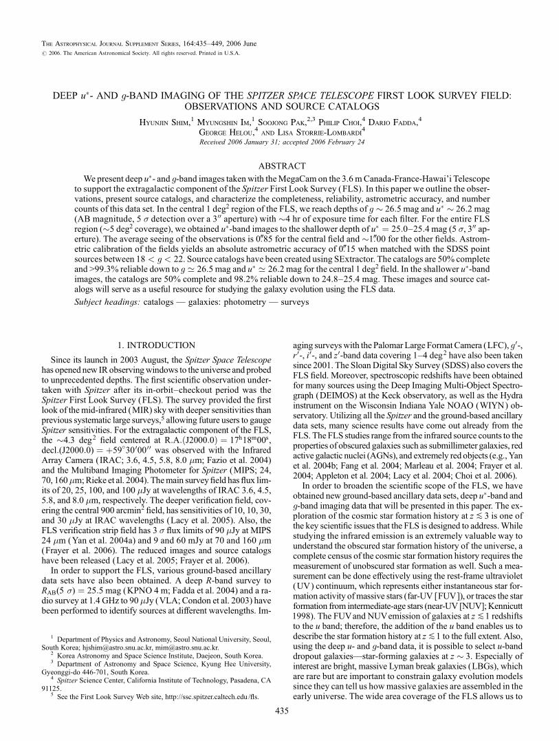
The observations were made using the MegaCam on the3.6 m Canada France Hawaii Telescope (CFHT). MegaCamconsists of 36 2048 ; 4612 pixel CCDs, covering 0N96 ; 0N94field of view with a resolution of 0B187 pixel�1 (see the detaileddescription in Boulade et al. 2003). The available broadbandfilters are similar to SDSS ugriz filters, but not exactly the same,especially in the case of the u� band. We used u� and g filters forour observations. The filter characteristics are summarized inTable 1, and their response curves are compared with the SDSSu- and g-band filters in Figure 1. Note that these response curvesinclude the quantum efficiency of the CCDs. The response curvesof the two g bands are nearly identical in their shapes, but theu�-band response curve shows a different overall shape com-pared with the SDSS u band, in such a sense that the u� filter isredder than SDSS u. The difference leads to as much as a 0.6magdifference between the CFHTand SDSS umagnitudes. This willbe investigated further in the photometry section (x 5.2).

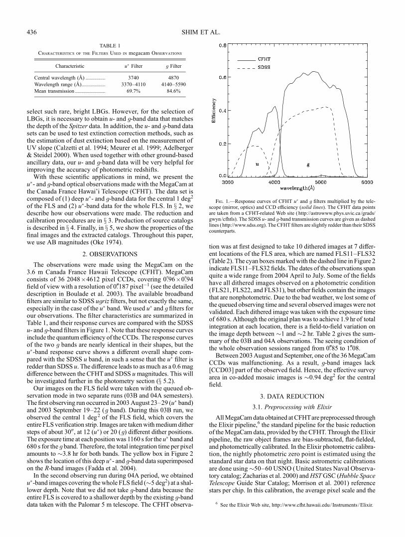
Our images on the FLS field were taken with the queued ob-servation mode in two separate runs (03B and 04A semesters).The first observing run occurred in 2003August 23–29 (u� band)and 2003 September 19–22 (g band). During this 03B run, weobserved the central 1 deg2 of the FLS field, which covers theentire FLS verification strip. Images are takenwithmedium dithersteps of about 3000, at 12 (u�) or 20 (g) different dither positions.The exposure time at each positionwas 1160 s for the u� band and680 s for the g band. Therefore, the total integration time per pixelamounts to �3.8 hr for both bands. The yellow box in Figure 2shows the location of this deep u�- and g-band data superimposedon the R-band images (Fadda et al. 2004).

In the second observing run during 04A period, we obtainedu�-band images covering the whole FLS field (�5 deg2) at a shal-lower depth. Note that we did not take g-band data because theentire FLS is covered to a shallower depth by the existing g-banddata taken with the Palomar 5 m telescope. The CFHT observa-

tion was at first designed to take 10 dithered images at 7 differ-ent locations of the FLS area, which are named FLS11–FLS32(Table 2). The cyan boxesmarkedwith the dashed line in Figure 2indicate FLS11–FLS32 fields. The dates of the observations spanquite a wide range from 2004 April to July. Some of the fieldshave all dithered images observed on a photometric condition(FLS21, FLS22, and FLS31), but other fields contain the imagesthat are nonphotometric. Due to the bad weather, we lost some ofthe queued observing time and several observed images were notvalidated. Each dithered image was taken with the exposure timeof 680 s. Although the original plan was to achieve 1.9 hr of totalintegration at each location, there is a field-to-field variation onthe image depth between �1 and �2 hr. Table 2 gives the sum-mary of the 03B and 04A observations. The seeing condition ofthe whole observation sessions ranged from 0B85 to 1B08.Between 2003August and September, one of the 36MegaCam

CCDs was malfunctioning. As a result, g-band images lack[CCD03] part of the observed field. Hence, the effective surveyarea in co-added mosaic images is �0.94 deg2 for the centralfield.

3. DATA REDUCTION

3.1. Preprocessing with Elixir

AllMegaCamdata obtained at CFHTare preprocessed throughthe Elixir pipeline,6 the standard pipeline for the basic reductionof theMegaCam data, provided by the CFHT. Through the Elixirpipeline, the raw object frames are bias-subtracted, flat-fielded,and photometrically calibrated. In the Elixir photometric calibra-tion, the nightly photometric zero point is estimated using thestandard star data on that night. Basic astrometric calibrationsare done using�50–60 USNO (United States Naval Observa-tory catalog; Zacharias et al. 2000) andHSTGSC (Hubble SpaceTelescope Guide Star Catalog; Morrison et al. 2001) referencestars per chip. In this calibration, the average pixel scale and the

TABLE 1

Characteristics of the Filters Used in megacam Observations

Characteristic u� Filter g Filter

Central wavelength (8) ............... 3740 4870

Wavelength range (8).................. 3370–4110 4140–5590

Mean transmission ....................... 69.7% 84.6%

Fig. 1.—Response curves of CFHT u� and g filters multiplied by the tele-scope (mirror, optics) and CCD efficiency (solid lines). The CFHT data pointsare taken from a CFHT-related Web site ( http://astrowww.phys.uvic.ca /grads/gwyn /cfhtls). The SDSS u- and g-band transmission curves are given as dashedlines (http://www.sdss.org). The CFHT filters are slightly redder than their SDSScounterparts.

6 See the Elixir Web site, http://www.cfht.hawaii.edu / Instruments /Elixir.

SHIM ET AL.436

Fig. 2.—Area coverages of various data sets over the FLS. The small yellow square in the center represents the Spitzer FLS verification strip, and the big yellowsquare shows our CFHTobservations in the central 1 deg2. The red and white squares correspond to the whole FLS area (IRAC and MIPS, respectively), which covers�4.3 deg 2. The cyan squares indicate the area covered by our CFHT u�-band observations in 2004. All these marks are overlaid on the KPNO R-band images.

TABLE 2

Observation Summary

Field ID R. A. (J2000.0) Decl. (J2000.0) Observation Dates Filter

Total Exposure Time

(s)

Depth

(AB mag)aSeeing

(arcsec)b Zero Pointc

Central ........... 17 17 01 +59 45 08 2003 Aug 25, 2003 Aug 29 u� 1160 ; 12 26.41 0.85 32.904

Central ........... 17 17 01 +59 45 08 2003 Sep 19, 2003 Sep 21, 2003 Sep 22 g 680 ; 20 26.72 0.85 33.430

FLS11............ 17 22 09 +60 14 47 2004 Apr 29, 2004 Jul 12 u� 680 ; 10 25.83 0.98 32.226

FLS12............ 17 14 44 +60 14 50 2004 Jun 18, 2004 Jul 17 u� 680 ; 9 25.85 1.06 32.186

FLS21............ 17 22 14 +59 30 00 2004 Jul 10, 2004 Jul 21 u� 680 ; 9 25.91 0.98 32.236

FLS22............ 17 14 47 +59 44 45 2004 Jul 10 u� 680 ; 5 25.57 1.08 32.213

FLS23............ 17 07 09 +59 48 26 2004 Jul 11 u� 680 ; 5 25.43 0.89 32.221

FLS31............ 17 20 46 +58 49 09 2004 Jul 11, 2004 Jul 22 u� 680 ; 8 25.68 0.90 32.188

FLS32............ 17 13 32 +58 57 46 2004 Jul 12 u� 680 ; 7 25.67 0.95 32.139

Note.—Units of right ascension are hours, minutes, and seconds, and units of declination are degrees, arcminutes, and arcseconds.a The depth of a field is calculated as 5 � flux over a 300 aperture.b The seeing of the image was determined through a visual inspection of individual stars.c The zero points are calibrated from original Elixir photometric solution (see x 3.5). The values are given as zero points according to DN.

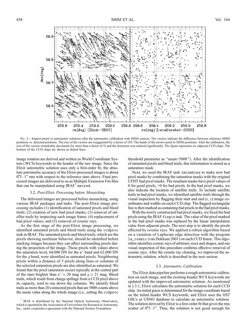
image rotation are derived and written as World Coordinate Sys-tem (WCS) keywords to the header of the raw image. Since theElixir astrometric solution uses only a first-order fit, the abso-lute astrometric accuracy of the Elixir-processed images is about0B5–100 rms with respect to the reference stars above. Final pro-cessed images are delivered to us as Multiple Extension Fits filesthat can be manipulated using IRAF7 mscred.

3.2. Post-Elixir Processing before Mosaicking

The delivered images are processed before mosaicking, usingvarious IRAF packages and tasks. The post-Elixir image pro-cessing includes (1) identification of saturated pixels and bleedtrails; (2) creation of new bad pixel masks; (3) removal of sat-ellite trails by inspecting each image frame; (4) replacement ofbad pixel values; and (5) removal of cosmic rays.

As the first stage of the post-Elixir image processing, weidentified saturated pixels and bleed trails using the ccdproctask in IRAF. The saturated pixels and bleed trails, which are thepixels showing nonlinear behavior, should be identified beforestacking images because they can affect surrounding pixels dur-ing the projection of the image. Those pixels with values abovethe saturation level, 64,000 DN for the u� band and 62,000 DNfor the g band, were identified as saturated pixels. Neighboringpixels within a distance of 5 pixels along lines or columns ofthe selected saturation pixels are also identified as saturated.Wefound that the pixel saturation occurs typically at the central partof the stars brighter than u� ’ 20 mag and g ’ 21 mag. Bleedtrails, which result from charge spillage from a CCD pixel aboveits capacity, tend to run down the columns. We identify bleedtrails as more than 20 connected pixels that are 5000 counts abovethe mean value along the whole image (i.e., setting the ccdproc

threshold parameter as ‘‘mean+5000’’). After the identificationof saturated pixels and bleed trails, this information is stored as asaturation mask.Next, we used the IRAF task imcombine to make new bad

pixel masks by combining the saturation masks with the originalCFHT bad pixel masks. The resultant masks have pixel values of0 for good pixels, >0 for bad pixels. In the bad pixel masks, wealso indicate the location of satellite trails. To include satellitetrails in bad pixel masks, we identified satellite trails through thevisual inspection by flagging their start and end (x, y) image co-ordinates and widths on each CCD chip. The flagged rectangularline is thenmarked as containing bad pixels in the bad pixelmasks.With the newly constructed bad pixel masks, we fixed the bad

pixels using the IRAF fixpix task. The value of the pixel markedin the bad pixel masks was replaced by the linear interpolationvalue from adjacent pixels. The next step is to identify the pixelsaffected by cosmic rays. We applied a robust algorithm basedon a variation of Laplacian edge detection with the programla_cosmic (van Dokkum 2001) on each CCD frame. This algo-rithm identifies cosmic rays of arbitrary sizes and shapes, and ourvisual inspection of this procedure confirms effective removal ofcosmic rays. After the cosmic ray cleaning, we improved the as-trometric solution, which is described in the next section.

3.3. Astrometric Calibration

The Elixir data pipeline performs a rough astrometric calibra-tion on each image, and the existing header WCS keywords areupdated with the improved astrometric solution. As mentionedin x 3.1, Elixir calculates the astrometric solution for each CCDchip. An initial guess is determined for the image coordinate basedon the initial header WCS keywords, and Elixir uses the HSTGSCs or USNO database to calculate an astrometric solution.The solution derived by Elixir is a first-order fit that gives the rmsscatter of 0B5–100. Thus, the solution is not good enough for

7 IRAF is distributed by the National Optical Astronomy Observatory,which is operated by the Association of Universities for Research in Astronomy,Inc., under cooperative agreement with the National Science Foundation.

Fig. 3.—Improvement in astrometric solutions after the astrometric calibration with SDSS sources. The vectors indicate the difference between reference SDSSpositions vs. detected positions. The size of the vectors are exaggerated by a factor of 250. The heads of the arrows point to SDSS positions. After the calibration, thesize of the vectors remarkably decreased (by more than a factor of 5) and the distortion was reduced significantly. The figure represents six adjacent CCD chips. Theborders of the CCD chips are shown as dotted lines.

SHIM ET AL.438 Vol. 164

follow-up observations that require very accurate position infor-mation such as themultiobject spectroscopy. The accurate astrom-etry is also important when combining and mosaicking images,since misalignment of images can lead to a loss of signal in thecombined image.

To improve the astrometric solutions, we adopted SDSS sourcesas reference points and derived the astrometric solution using themsctpeak task in mscfinder, which is a subpackage of the IRAFmosaic reduction package mscred. The SDSS sources brighter

than r ’ 20 mag have an absolute astrometric accuracy of 0B045rms with respect to USNO catalogs (Zacharias et al. 2000) and0B075 rms against Tycho-2 catalogs (Hog et al. 2000), with an ad-ditional 0B02–0B03 systematic error in both cases (Pier et al. 2003).We also considered usingUSNO andGSC catalogs; unfortunately,many of the USNO and GSC stars were saturated in our images,making it difficult to use them for astrometric calibration.

There are other tasks such as msczero and msccmatch forderiving the astrometric solution, butwe settled onusingmsctpeak.

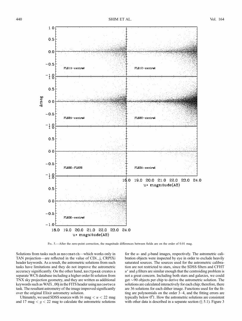
Fig. 4.—Magnitude difference of matched objects from different eight u�-band fields before zero-point correction. Note that the objects lying in the FLS21, FLS22, andFLS31 fields are brighter than the objects lying in the central field before zero-point correction. The mean value of the magnitude offsets are FLS11� central ’ 0:006,FLS12� central’ 0:018, FLS21� central’ �0:028,FLS22� central ’ �0:029, FLS22� FLS23’ �0:009, FLS31� central’ �0:035, andFLS32� central ’ �0:001.Since the magnitude offsets of the FLS21, FLS22, and FLS31 fields are consistent within 0.01 mag, we used these fields as zero-point reference fields.

SPITZER FIRST LOOK SURVEY FIELD 439No. 2, 2006

Solutions from tasks such as msccmatch—which works only inTAN projection—are reflected in the value of CDi_ j, CRPIXiheader keywords. As a result, the astrometric solutions from suchtasks have limitations and they do not improve the astrometricaccuracy significantly. On the other hand, msctpeak creates aseparateWCS database including a higher order fit solution fromTNX sky projection geometry, and they are written as additionalkeywords such asWATi_00j in the FITS header usingmscsetwcstask. The resultant astrometry of the image improved significantlyover the original Elixir astrometry solution.

Ultimately,we used SDSS sourceswith 16 mag < u < 22 magand 17 mag < g < 22 mag to calculate the astrometric solutions

for the u- and g-band images, respectively. The astrometric cali-bration objects were inspected by eye in order to exclude heavilysaturated sources. The sources used for the astrometric calibra-tion are not restricted to stars, since the SDSS filters and CFHTu� and g filters are similar enough that the centroiding problem isnot a great concern. Including both stars and galaxies, we couldget �90 objects per chip to derive the astrometric solution. Thesolutions are calculated interactively for each chip; therefore, thereare 36 solutions for each dither image. Functions used for the fit-ting are polynomials on the order 3–4, and the fitting errors aretypically below 0B1. How the astrometric solutions are consistentwith other data is described in a separate section (x 5.1). Figure 3

Fig. 5.—After the zero-point correction, the magnitude differences between fields are on the order of 0.01 mag.


demonstrates the improvement of astrometric solutions after exe-cuting the above procedure.

3.4. Production of Mosaic Images

We stacked the post-Elixir processed, astrometrically calibratedimages using Swarp software by E. Bertin at TERAPIX (TraitmentElementaire, Reduction et Analyze des Pixels demegacam). 8 Byrunning Swarp, we created themosaic image and the correspond-ing weight image (coverage map) whose pixel value is propor-tional to the exposure time. The reduced images were resampled,background-subtracted, flux-scaled, and finally co-added to oneimage. The interpolation function we used in the resampling wasLANCZOS3, which uses a moderately large kernel. The pixelscale of the resampled image was kept to the original MegaCampixel size of 0B185. The astrometry transformation was handledby the Swarp program automatically, although the TNXWCS asderived in the previous section is not a FITS standard.

For the background subtraction, we used the backgroundmesh size of 128 ; 128 pixels and applied a 3 ; 3 filter box. Thebackground mesh size and the bin size were chosen to balanceout the effect of bright stars (in general, smaller than 128 ; 128pixels) and the effect of the overall background gradient. Wetriedmany background combinations to obtain a background thatwas as flat as possible and settled on the above parameter values.The background-subtracted images were combined by taking theweighted average of each frame. The weight images were con-structed by taking the bad pixel masks and replacing the bad pixelvalues with 0 and the good pixel values with be 1. Theweight im-ages constructed in this way do not account for small variation inthe pixel response over the CCD (flat field). Finally, the imageswere co-added using the following equation:

F ¼P

wi pi fiPwi

:

In this equation, F is the value of a pixel in the final co-addedimage, wi is the weight value for the pixel, and fi is the value ofthe pixel in each individual image. The factor pi represents theflux scale for each individual image. The images are calibratedto have the same photometric zero points after the Elixir pipeline,but due to the air mass differences, the flux scales of the imagesare slightly different. In order to take into account the differencein zero points, we set the flux scale of the image with the lowestextinction as 1.0. The flux scales of other images were calculatedaccording to the equation

pi ¼ 10( k=2:5)(Xi�X0);

where k is the coefficient for the air mass term and X0 and Xi areair mass values of the reference image and the image in consid-eration, respectively. The co-added gain of the final stacked im-age varieswith position and is proportional to the number offramesused for producing each co-added pixel value.

3.5. Photometric Calibration

We performed photometric calibration on the mosaic image ofeach field using the photometric solution provided by the Elixirpipeline. During the production of mosaic images (x 3.4), we re-scaled each dithered image so that each co-added image has thephotometric zero point of the image with the lowest air massvalue. Then these magnitudes were corrected for Galactic extinc-tion, estimating the amount of Galactic extinction from the ex-

tinction map of Schlegel et al. (1998). Since the FLS field lies atmoderately high Galactic latitude, the amount of Galactic ex-tinction is relatively small. They are 0.15 and 0.1mag on averagefor the u� and g bands, respectively. In the next step, we derivedan additional zero-point correction necessary to account for someof the data that were taken under nonphotometric condition (e.g.,thin cirrus).

To do so in the u� band, we used fields whose mosaic imageis made of photometric dither images only. The fields FLS21,FLS22, and FLS31 are such fields, and we used them as reference

Fig. 6.—Distribution of the values of CLASS_STAR parameter as a func-tion of magnitude. At magnitudes below flux limit, the stellarity index of theobjects is distributed between 0.35 and 0.7. The feature of the CLASS_STARdistribution at faint objects (�27 mag) is due to the difficulties when calculat-ing stellarity index with isophotal areas of the objects.

8 See http://terapix.iap.fr.


photometry fields to derive photometric zero-point correc-tion of other u�-band fields. Figure 4 shows the comparison ofu�-band magnitudes (before correcting for the nonphotomet-ric data) between different fields that overlap with each other.For the comparison of magnitudes, we used the total magnitude(MAG_AUTO) from SExtractor (see x 4). In Figure 4, we cansee that u�-band magnitudes of objects in FLS21, FLS22, andFLS31 fields are slightly brighter than the same objects in thecentral field. Also, objects in fields other than the reference pho-tometry fields have u�-band magnitudes similar to or fainter thanthose of the central field. The u�-magnitude offsets between thecentral field and FLS21/FLS22/FLS31 are 0.03mag and the rmsin the offset values is on the order of P0.01 mag. This confirmsthat the u�-band magnitudes of FLS21/FLS22/FLS31 fields arethe most reliable. The final u�-band zero points of each field arecalculated using this strategy, and we present the zero points inTable 2. The comparison of u�-band magnitudes of overlappingobjects after the photometric calibration are presented in Figure 5.On the basis of the photometric consistency between FLS21/FLS22/FLS31, we estimate the accuracy of the u�-band photo-metric zero point to be on the order of 0.01 mag.

For the g-band mosaic, we performed photometry on ditherimages that were taken under photometric conditions and deriveda necessary zero-point correction by comparing the photometryof the mosaic image and the photometric reference image. Theg-band zero point of the central field derived this way is alsogiven in Table 2.

4. CATALOGS

4.1. Object Detection and Photometry

In the central 1 deg2 region (the 03B run), the stacked u�- andg-band images were registered to the g-band image. Both bandshave the same pixel scale, so they can be easily registered withthe xregister task in IRAF. After the registration, source cat-alogs were created using dual-mode photometry with SExtractor(Bertin & Arnouts 1996). Specifically, objects were detected inthe g-band image, and photometry was performed on both theg- and u�-band images based on these positions. The weight

image (coverage map) produced by Swarp was used as theWEIGHT_IMAGE. The LOCAL background is estimated us-ing a 128 ; 128 pixel backgroundmeshwith 3 ; 3median boxcarfiltering, identical to the default Swarp settings.We filtered our images with a Gaussian convolution kernel

(gauss_4.0_7;7.conv) matched to our average seeing condi-tions (FWHM � 0B85). Finally, source detection was performedon the background-subtracted, filtered image by looking for pixelgroups above the detection threshold. After playing with variousparameter combinations and inspecting the results by eye, we set-tled on a minimum of eight connected pixels and a 1.2 � mini-mum detection threshold. We also tried various values for thedeblending parameter to separate objects that are close together,

TABLE 3

Selected 15 Entries of u�/g Band Source Catalog

ID R.A. (J2000.0) Decl. (J2000.0) u�AUTOa � u�APER

b � gAUTO � gAPER � Stargc Extu�

d Extg

1001..................... 17 14 13.301 59 15 19.199 24.992 0.051 25.016 0.042 24.726 0.066 24.699 0.052 0.010 0.120 0.088

1002..................... 17 17 11.895 59 15 27.342 24.882 0.043 25.200 0.052 24.834 0.063 25.112 0.073 0.006 0.169 0.125

1003..................... 17 15 52.126 59 15 26.820 24.872 0.040 25.184 0.048 24.796 0.053 25.135 0.064 0.086 0.151 0.111

1004..................... 17 13 19.966 59 15 16.411 24.955 0.050 25.408 0.061 24.582 0.069 25.144 0.092 0.024 0.114 0.084

1005..................... 17 19 55.115 59 15 21.739 25.356 0.080 25.615 0.070 25.364 0.064 25.744 0.063 0.928 0.141 0.104

1006..................... 17 14 53.745 59 15 25.502 25.628 0.088 26.223 0.156 25.666 0.071 26.027 0.102 0.586 0.124 0.092

1007..................... 17 13 55.459 59 15 21.272 25.644 0.091 26.233 0.123 25.627 0.072 26.334 0.109 0.232 0.118 0.087

1008..................... 17 18 35.120 59 15 27.905 26.073 0.138 27.508 0.390 26.164 0.110 28.560 0.752 0.725 0.158 0.116

1009..................... 17 15 37.141 59 15 28.592 26.565 0.189 26.240 0.122 26.578 0.181 26.348 0.128 0.693 0.146 0.107

1010..................... 17 15 33.977 59 15 19.844 23.060 0.009 24.161 0.019 22.738 0.013 23.741 0.026 0.028 0.145 0.106

1011..................... 17 14 33.853 59 15 19.858 23.000 0.008 23.381 0.010 22.917 0.011 23.295 0.013 0.048 0.121 0.089

1012..................... 17 17 52.075 59 15 25.035 23.869 0.018 24.589 0.030 23.858 0.037 24.674 0.068 0.029 0.180 0.132

1013..................... 17 18 54.719 59 15 23.401 23.485 0.013 23.992 0.016 23.444 0.015 23.960 0.019 0.959 0.148 0.109

1014..................... 17 16 11.917 59 15 26.175 23.960 0.018 24.495 0.025 23.890 0.023 24.382 0.031 0.036 0.153 0.113

1015..................... 17 17 19.797 59 15 29.375 26.003 0.113 26.299 0.139 26.031 0.169 26.255 0.194 0.131 0.172 0.127

Note.—Units of right ascension are hours, minutes, and seconds, and units of declination are degrees, arcminutes, and arcseconds.a The AUTO magnitudes are calculated by SExtractor, using Kron-like elliptical apertures (Kron 1980).b The APER magnitudes are calculated over a circle with 300 diameter.c The stellarity represents CLASS_STAR calculated with SExtractor. The values are distributed between 0 (galaxy) and 1 (star).d The Galactic extinction values are calculated using the extinction map of Schlegel et al. (1998).

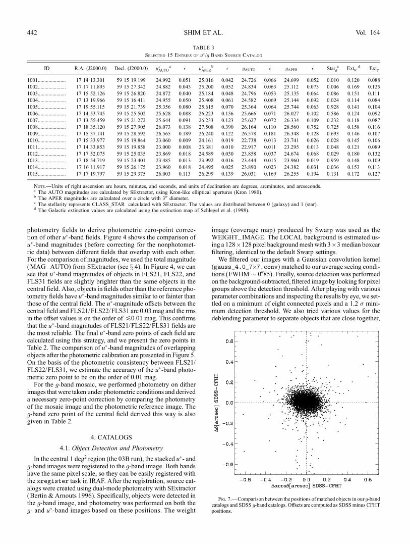
Fig. 7.—Comparison between the positions of matched objects in our g-bandcatalogs and SDSS g-band catalogs. Offsets are computed as SDSS minus CFHTpositions.


and we adopted a deblending threshold of 32 and a deblendingminimal contrast of 0.005.

Using dual-mode photometry, we detect�200,000 sources inthe central 1 deg2 field. We also performed single-mode photom-etry on the u�-band image with the same configuration file, to in-clude u�-band objects that are not detected in the g band. About�150 objects were detected in the u� band without detection inthe g band.

We applied a nearly identical method and parameters forsource detection on the seven 04A FLS u�-band images. Sincethere are several very bright stars in the 04A u�-band images,we chose a bigger background mesh size, 256 ; 256 pixels, toavoid the oversubtraction of the background near bright stars.Since the seeing during 04Awas slightly worse than that of 03B(Table 2), we adopted a slightly larger Gaussian convolutionkernel (gauss_5.0_9;9.conv). As stated earlier, the gain foreach stacked image is determined to be the original gain timesthe number of stacked images.

Due to interchip gaps and our 3000–4000 dither steps, the effec-tive exposure time varies from pixel to pixel. We therefore ap-plied the Swarp weight image when performing photometry.Through the visual inspection of the weight image, we deter-mined the value ofWEIGHT_THRESH parameter for weightingin SExtractor. The value of the pixels in interchip gaps weremeasured and used as the threshold parameter value. This pro-cedure prevents the rise of unusual sequence in the magnitudeversus magnitude error plot.

In the catalogs, we present the apparent magnitude of the ob-jects in two different ways (aperture and total magnitude). Wemeasured the aperture magnitude using a 300 diameter apertures.We adopted the automagnitude (MAG_AUTO ) from SExtractoras the total magnitude, which is calculated using the Kron el-liptical aperture (Kron 1980). The related parameters, PHOT_

AUTOPARAMS were determined to be 2.5 and 3.5, which arethe values in the default configuration file.

4.2. Star-Galaxy Separation

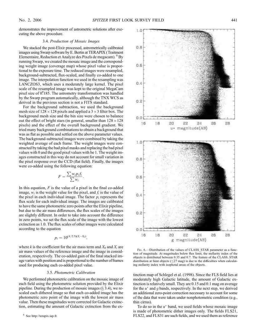
We use the SExtractor stellarity index to separate starlike ob-jects from extended sources. SExtractor uses eight measured iso-photal areas, peak intensity, and seeing information to calculate

the stellarity index.With the SEEING_FWHMparameter valueand the neural network file as the inputs, SExtractor gives thestellarity index (CLASS_STAR), which has values between 1(starlike object) and 0 as the result of the classification. Figure 6shows the distribution of stellarity index as a function of mag-nitude in the central 1 deg2 field. We randomly picked objectswith different apparent magnitudes and stellarity index values,and visually inspected them to see how useful the stellartiy in-dex is for the point source versus extended source classification.Our visual inspection reveals that bright objects (g < 21 mag,and u� < 20 mag) with the stellarity index k0.8 are found tobe stars. Through the visual inspection, we adopted the follow-ing criteria for separating point sources from extended objects:CLASS_STAR > 0.8 for 20 < u� < 23; CLASS_STAR > 0.8for 21 < g < 23.

In addition to these criteria, we weed out bright saturatedstars (g < 21 mag, u� < 20 mag), based on SDSS point sourcecatalogs. The subtraction of objects matched with SDSS stars isa good method for removing stars from our catalogs.

On the other hand, it is difficult to address the nature of faint(g > 23 mag, u� > 23 mag) objects with the stellarity valuealone, because faint, distant small galaxies are hardly resolvedunder 100 seeing conditions. Fortunately, number counts tend tobe dominated by galaxies at u�; g > 23 mag. Therefore, we donot attempt to separate stars from galaxies at these flux levels.Also, the stellarity index distribution shows a converging fea-ture between 0.35 and 0.7 at magnitudes below flux limit (g >26:5 mag, u� > 26:2 mag). This is thought to be the effect ofdifficulties in determining isophotal areas of faint objects.

4.3. Catalog Formats

As an example, 15 entries of the central 1 deg2 u�- andg-band merged catalog is presented in Table 3. All magnitudesare given in the AB magnitude system. We include the total mag-nitude (MAG_AUTO) and the aperture magnitude (300 diameter)in the catalog. The magnitudes are not corrected for Galactic ex-tinction, but the extinction values are presented as a separatecolumn. Magnitude errors are the outputs from SExtractor. Con-sidering the error in zero point and the extinction correction, webelieve that the minimal error in the magnitude will be about

Fig. 8.—Comparison between the positions of matched objects in our u�-band catalogs and R-band, IRAC catalogs. The offsets are computed as other survey minusCFHT positions.


0.02 mag. Stellarity indices are calculated in the g-band imagefor the central field.

5. PROPERTIES OF THE DATA

5.1. Astrometry

We derived the final astrometric solution using SDSS sources(both point and extended sources). The rms error between SDSSpoint sources and our sources is calculated to be 0B1 < dr <0B15. Considering the absolute astrometric error of 0B1 in SDSS(Pier et al. 2003), our catalogs are thought to have the positionalerror of roughly 0B15–0B2. Figure 7 shows the positional differ-ences between SDSS sources and our sources over the entiremosaic of the central 1 deg2 field.

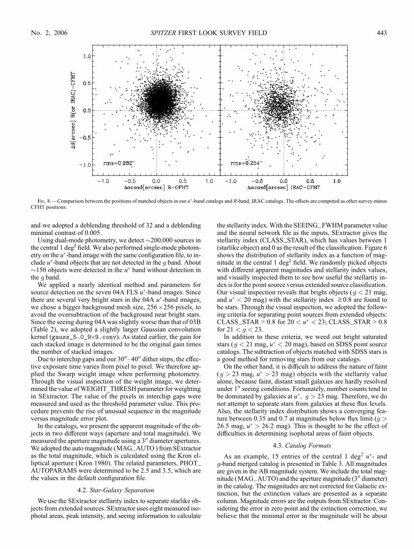
To address the accuracy of astrometric calibration in otherways, we compared our source positions with other availablecatalogs for the Spitzer FLS. The catalogs compared are KPNOR-band data (Fadda et al. 2004) and the Spitzer IRAC data (Lacyet al. 2005). The results are given in Figure 8. The average rmserror, dr ¼ (�� cos � 2 þ�� 2)1

=2, is about�0B28 with respectto R-band data. R-band positions have a systematic offset of�� ¼ 0B09 � 0B27 and�� ¼ 0B19 � 0B31with respect toCFHTpositions. The systematic offset is originated from the fact thatthe reference catalog for R-band data is GSC II stars, which isknown to have a systematic offset with respect to SDSS referencepositions (Fadda et al. 2004). Therefore, we consider the astrom-etry difference between R-band and CFHT data to be well un-derstood. For IRAC sources, the average rms error is dr ’ 0B25.The offset of IRAC positions according to CFHT positions arecalculated to be �� ¼ �0B08 � 0B40 and �� ¼ 0B04 � 0B38.The FLS IRAC data have positional accuracy of 0B25 rms withrespect to 2MASS (Lacy et al. 2005). The difference between2MASS positions and SDSS positions caused the offset be-tween IRAC positions and CFHT positions. The results add sup-port to the astrometric accuracy of our data set.

5.2. Photometry Transformation

As we have shown in Figure 1, MegaCam filters are slightlyredder than their SDSS counterparts. Therefore, we examinedthe correlations between u� magnitudes and SDSS umagnitudes.To do so, we matched nonsaturated point sources with 18:5 <u < 20 from our catalog with the SDSS point source catalog andcompared the differences in their magnitudes. Figure 9 showsthe comparison, and it demonstrates that the difference betweenthe u� and u bands varies from 0.1 to 0.6 mag as a function of thecolor of the object. We fitted the relation with a first-order poly-nomial to construct the conversion formula between CFHT u�

and SDSS u-band magnitudes and obtained the following re-lation from the linear least-squares fitting. Although there existssome scatter, the conversion formula could be a good referencein use of CFHT u� magnitude:

�mag(uSDSS � uCFHT)¼ (�0:081 � 0:006)

þ (0:237 � 0:004)(u� g)SDSS:

We checked the above empirical relation between MegaCam u�

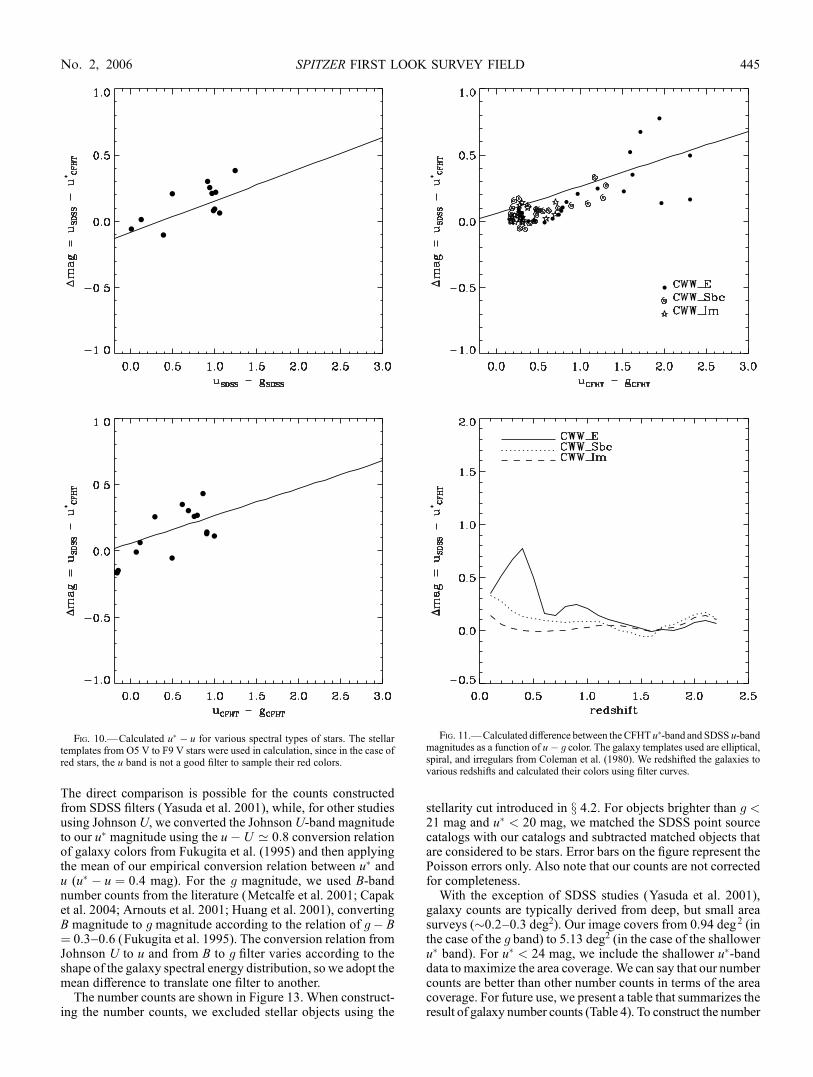
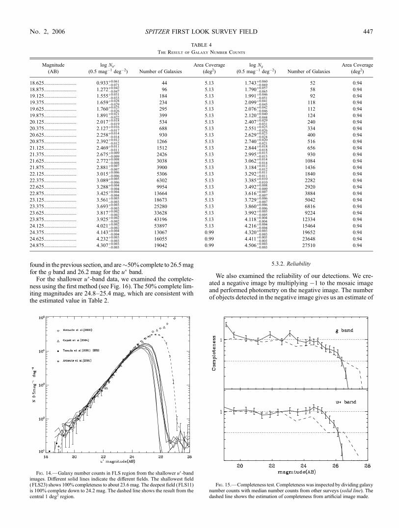
and SDSS u by calculating u� � u versus u� g using the filtercurves in Figure 1 and the stellar templates from O5 V to F9 Vstars (Silva & Cornell 1992), or the empirical galaxy templatesat different redshift (Coleman et al. 1980). The theoreticallycalculated relations of u� � u versus u� g agree well with theempirical relations (Figs. 10 and 11).

On the other hand, the difference between SDSS g-bandmag-nitude and CFHT g-band magnitude is considerably small. Fig-

ure 12 shows their difference along u� g color. Compared toFigure 9, the magnitude difference is small (they scatter within0.15 mag), but the differences still have a tendency of increas-ing toward red color. We applied a least-squares fit to the g-bandmagnitude difference to find the following conversion relation:

�mag(gSDSS � gCFHT) ¼ (�0:061 � 0:007)

þ (0:057 � 0:004)(u� g)SDSS:

5.3. Galaxy Number Counts

To show the depth and homogeneity of the survey, we pre-sent the galaxy number counts in the u� and g bands. The num-ber counts are constructed for both the deep central 1 deg2 fieldand the shallower u�-band coverage of the entire FLS fields. Thenthe results are compared with galaxy counts from other studies.

Fig. 9.—Empirical difference between CFHT u�-band and SDSS u-bandmag-nitudes as a function of u� g color. We used a least-squares fit to find the con-version equation from one u band to another.


The direct comparison is possible for the counts constructedfrom SDSS filters (Yasuda et al. 2001), while, for other studiesusing Johnson U, we converted the Johnson U-band magnitudeto our u� magnitude using the u� U ’ 0:8 conversion relationof galaxy colors from Fukugita et al. (1995) and then applyingthe mean of our empirical conversion relation between u� andu (u� � u ¼ 0:4 mag). For the g magnitude, we used B-bandnumber counts from the literature (Metcalfe et al. 2001; Capaket al. 2004; Arnouts et al. 2001; Huang et al. 2001), convertingB magnitude to g magnitude according to the relation of g� B¼ 0:3 0:6 (Fukugita et al. 1995). The conversion relation fromJohnson U to u and from B to g filter varies according to theshape of the galaxy spectral energy distribution, so we adopt themean difference to translate one filter to another.

The number counts are shown in Figure 13. When construct-ing the number counts, we excluded stellar objects using the

stellarity cut introduced in x 4.2. For objects brighter than g <21 mag and u� < 20 mag, we matched the SDSS point sourcecatalogs with our catalogs and subtracted matched objects thatare considered to be stars. Error bars on the figure represent thePoisson errors only. Also note that our counts are not correctedfor completeness.

With the exception of SDSS studies (Yasuda et al. 2001),galaxy counts are typically derived from deep, but small areasurveys (�0.2–0.3 deg2). Our image covers from 0.94 deg2 (inthe case of the g band) to 5.13 deg2 (in the case of the shalloweru� band). For u� < 24 mag, we include the shallower u�-banddata to maximize the area coverage. We can say that our numbercounts are better than other number counts in terms of the areacoverage. For future use, we present a table that summarizes theresult of galaxy number counts (Table 4). To construct the number

Fig. 11.—Calculated difference between the CFHT u�-band and SDSS u-bandmagnitudes as a function of u� g color. The galaxy templates used are elliptical,spiral, and irregulars from Coleman et al. (1980). We redshifted the galaxies tovarious redshifts and calculated their colors using filter curves.

Fig. 10.—Calculated u� � u for various spectral types of stars. The stellartemplates from O5 V to F9 V stars were used in calculation, since in the case ofred stars, the u band is not a good filter to sample their red colors.


counts, we use the auto magnitude in SExtractor. Our numbercounts are in good agreement with the counts from other studiesto u� ’ 24:8 mag and g ’ 25:2 mag. Beyond u� ’ 24:8 magand g ’ 25:2 mag, our data start to tail off, and this shows thatour u� and g catalogs are nearly 100%complete down to the abovemagnitude limits. These limiting magnitudes have the uncertaintyof 0.3 mag due to the fluctuation in the galaxy number counts atthe faint end. We also obtained the number counts for the shal-lower u�-band data, and the results are illustrated in Figure 14.In the case of the deepest field among the shallower u� band, the100% limit is 24.2 mag.

5.3.1. Completeness

To inspect the completeness of our survey in more detail, weused two independent methods. First, we compared our galaxy

counts with the deeper galaxy counts from other studies. Second,we made artificial images having the same properties with ourobservation (seeing, crowding, gain, and background) using theartdata package in IRAF. The artificial image contained bothpoint sources and extended sources. The extended sources are de-fined to have 40% of whole galaxies as elliptical galaxies and theremainders for disk galaxies, withminimum redshift of z ’ 0:01.Poisson noise is added to the background. Then we performedphotometry with the same configuration file we used to makecatalogs of observed sources.The results are shown in Figure 15, where the solid line and

points indicate the completeness from the first method and thedashed line represents the completeness estimated from the sim-ulation. Figure 15 shows that the data are 100% complete downto g ’ 25:2mag and u� ’ 24:8mag, in agreement with the value

Fig. 13.—Galaxy number counts in FLS region from our u�- and g-bandimages. Results from other studies are overplotted.Magnitudes are in AB system.

Fig. 12.—Empirical difference of CFHT g-bandmagnitude and SDSS g-bandmagnitude according to u� g color. Because the CFHT filter is redder than theSDSSfilter, there is also a small tendency ofmagnitude difference along the color.But it is not difficult to say that the difference is negligible.


found in the previous section, and are�50%complete to 26.5magfor the g band and 26.2 mag for the u� band.

For the shallower u�-band data, we examined the complete-ness using the first method (see Fig. 16). The 50% complete lim-iting magnitudes are 24.8–25.4 mag, which are consistent withthe estimated value in Table 2.

5.3.2. Reliability

We also examined the reliability of our detections. We cre-ated a negative image by multiplying �1 to the mosaic imageand performed photometry on the negative image. The numberof objects detected in the negative image gives us an estimate of

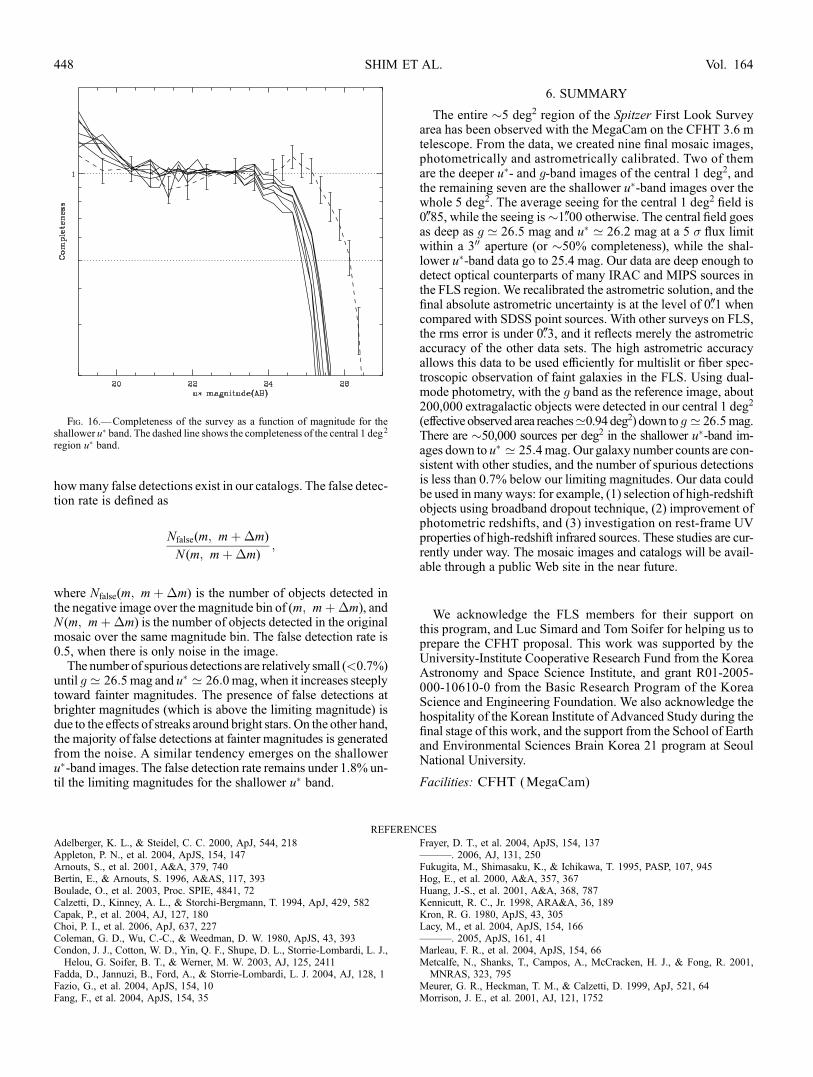
TABLE 4

The Result of Galaxy Number Counts

Magnitude

(AB)

log Nu�

(0.5 mag�1 deg�2) Number of Galaxies

Area Coverage

(deg2)

log Ng

(0.5 mag�1 deg�2) Number of Galaxies

Area Coverage

(deg2)

18.625......................... 0.933þ0:061�0:071 44 5.13 1.743þ0:060

�0:069 52 0.94

18.875......................... 1.272þ0:042�0:047 96 5.13 1.790þ0:057

�0:065 58 0.94

19.125......................... 1.555þ0:031�0:033 184 5.13 1.991þ0:046

�0:051 92 0.94

19.375......................... 1.659þ0:028�0:029 234 5.13 2.099þ0:041

�0:045 118 0.94

19.625......................... 1.760þ0:025�0:026 295 5.13 2.076þ0:042

�0:046 112 0.94

19.875......................... 1.891þ0:021�0:022 399 5.13 2.120þ0:040

�0:044 124 0.94

20.125......................... 2.017þ0:018�0:019 534 5.13 2.407þ0:029

�0:031 240 0.94

20.375......................... 2.127þ0:016�0:017 688 5.13 2.551þ0:025

�0:026 334 0.94

20.625......................... 2.258þ0:014�0:014 930 5.13 2.629þ0:023

�0:024 400 0.94

20.875......................... 2.392þ0:012�0:012 1266 5.13 2.740þ0:020

�0:021 516 0.94

21.125......................... 2.469þ0:011�0:011 1512 5.13 2.844þ0:018

�0:018 656 0.94

21.375......................... 2.675þ0:009�0:009 2426 5.13 2.995þ0:015

�0:015 930 0.94

21.625......................... 2.772þ0:008�0:008 3038 5.13 3.062þ0:014

�0:014 1084 0.94

21.875......................... 2.881þ0:007�0:007 3900 5.13 3.184þ0:012

�0:012 1436 0.94

22.125......................... 3.015þ0:006�0:006 5306 5.13 3.292þ0:011

�0:011 1840 0.94

22.375......................... 3.089þ0:005�0:006 6302 5.13 3.385þ0:010

�0:010 2282 0.94

22.625......................... 3.288þ0:004�0:004 9954 5.13 3.492þ0:008

�0:009 2920 0.94

22.875......................... 3.425þ0:004�0:004 13664 5.13 3.616þ0:007

�0:007 3884 0.94

23.125......................... 3.561þ0:003�0:003 18673 5.13 3.729þ0:006

�0:007 5042 0.94

23.375......................... 3.693þ0:003�0:003 25280 5.13 3.860þ0:006

�0:006 6816 0.94

23.625......................... 3.817þ0:002�0:002 33628 5.13 3.992þ0:005

�0:005 9224 0.94

23.875......................... 3.925þ0:002�0:002 43196 5.13 4.118þ0:004

�0:004 12334 0.94

24.125......................... 4.021þ0:002�0:002 53897 5.13 4.216þ0:004

�0:004 15464 0.94

24.375......................... 4.143þ0:004�0:004 13067 0.99 4.320þ0:003

�0:003 19652 0.94

24.625......................... 4.232þ0:003�0:003 16055 0.99 4.411þ0:003

�0:003 23648 0.94

24.875......................... 4.307þ0:003�0:003 19042 0.99 4.506þ0:003

�0:003 27510 0.94

Fig. 14.—Galaxy number counts in FLS region from the shallower u�-bandimages. Different solid lines indicate the different fields. The shallowest field(FLS23) shows 100% completeness to about 23.6 mag. The deepest field (FLS11)is 100% complete down to 24.2 mag. The dashed line shows the result from thecentral 1 deg2 region.

Fig. 15.—Completeness test. Completeness was inspected by dividing galaxynumber counts with median number counts from other surveys (solid line). Thedashed line shows the estimation of completeness from artificial image made.


howmany false detections exist in our catalogs. The false detec-tion rate is defined as

Nfalse(m; mþ�m)

N (m; mþ�m);

where Nfalse(m; mþ�m) is the number of objects detected inthe negative image over the magnitude bin of (m; mþ�m), andN (m; mþ�m) is the number of objects detected in the originalmosaic over the same magnitude bin. The false detection rate is0.5, when there is only noise in the image.

The number of spurious detections are relatively small (<0.7%)until g ’ 26:5mag and u� ’ 26:0mag, when it increases steeplytoward fainter magnitudes. The presence of false detections atbrighter magnitudes (which is above the limiting magnitude) isdue to the effects of streaks around bright stars. On the other hand,the majority of false detections at fainter magnitudes is generatedfrom the noise. A similar tendency emerges on the shalloweru�-band images. The false detection rate remains under 1.8% un-til the limiting magnitudes for the shallower u� band.

6. SUMMARY

The entire �5 deg2 region of the Spitzer First Look Surveyarea has been observed with the MegaCam on the CFHT 3.6 mtelescope. From the data, we created nine final mosaic images,photometrically and astrometrically calibrated. Two of themare the deeper u�- and g-band images of the central 1 deg2, andthe remaining seven are the shallower u�-band images over thewhole 5 deg2. The average seeing for the central 1 deg2 field is0B85, while the seeing is�1B00 otherwise. The central field goesas deep as g ’ 26:5 mag and u� ’ 26:2 mag at a 5 � flux limitwithin a 300 aperture (or �50% completeness), while the shal-lower u�-band data go to 25.4 mag. Our data are deep enough todetect optical counterparts of many IRAC and MIPS sources inthe FLS region. We recalibrated the astrometric solution, and thefinal absolute astrometric uncertainty is at the level of 0B1 whencompared with SDSS point sources. With other surveys on FLS,the rms error is under 0B3, and it reflects merely the astrometricaccuracy of the other data sets. The high astrometric accuracyallows this data to be used efficiently for multislit or fiber spec-troscopic observation of faint galaxies in the FLS. Using dual-mode photometry, with the g band as the reference image, about200,000 extragalactic objects were detected in our central 1 deg2

(effective observed area reaches’0.94deg2) down to g ’ 26:5mag.There are �50,000 sources per deg2 in the shallower u�-band im-ages down to u� ’ 25:4mag. Our galaxy number counts are con-sistent with other studies, and the number of spurious detectionsis less than 0.7% below our limiting magnitudes. Our data couldbe used inmanyways: for example, (1) selection of high-redshiftobjects using broadband dropout technique, (2) improvement ofphotometric redshifts, and (3) investigation on rest-frame UVproperties of high-redshift infrared sources. These studies are cur-rently under way. The mosaic images and catalogs will be avail-able through a public Web site in the near future.

We acknowledge the FLS members for their support onthis program, and Luc Simard and Tom Soifer for helping us toprepare the CFHT proposal. This work was supported by theUniversity-Institute Cooperative Research Fund from the KoreaAstronomy and Space Science Institute, and grant R01-2005-000-10610-0 from the Basic Research Program of the KoreaScience and Engineering Foundation. We also acknowledge thehospitality of the Korean Institute of Advanced Study during thefinal stage of this work, and the support from the School of Earthand Environmental Sciences Brain Korea 21 program at SeoulNational University.

Facilities: CFHT (MegaCam)

REFERENCES

Adelberger, K. L., & Steidel, C. C. 2000, ApJ, 544, 218Appleton, P. N., et al. 2004, ApJS, 154, 147Arnouts, S., et al. 2001, A&A, 379, 740Bertin, E., & Arnouts, S. 1996, A&AS, 117, 393Boulade, O., et al. 2003, Proc. SPIE, 4841, 72Calzetti, D., Kinney, A. L., & Storchi-Bergmann, T. 1994, ApJ, 429, 582Capak, P., et al. 2004, AJ, 127, 180Choi, P. I., et al. 2006, ApJ, 637, 227Coleman, G. D., Wu, C.-C., & Weedman, D. W. 1980, ApJS, 43, 393Condon, J. J., Cotton, W. D., Yin, Q. F., Shupe, D. L., Storrie-Lombardi, L. J.,Helou, G. Soifer, B. T., & Werner, M. W. 2003, AJ, 125, 2411

Fadda, D., Jannuzi, B., Ford, A., & Storrie-Lombardi, L. J. 2004, AJ, 128, 1Fazio, G., et al. 2004, ApJS, 154, 10Fang, F., et al. 2004, ApJS, 154, 35

Frayer, D. T., et al. 2004, ApJS, 154, 137———. 2006, AJ, 131, 250Fukugita, M., Shimasaku, K., & Ichikawa, T. 1995, PASP, 107, 945Hog, E., et al. 2000, A&A, 357, 367Huang, J.-S., et al. 2001, A&A, 368, 787Kennicutt, R. C., Jr. 1998, ARA&A, 36, 189Kron, R. G. 1980, ApJS, 43, 305Lacy, M., et al. 2004, ApJS, 154, 166———. 2005, ApJS, 161, 41Marleau, F. R., et al. 2004, ApJS, 154, 66Metcalfe, N., Shanks, T., Campos, A., McCracken, H. J., & Fong, R. 2001,MNRAS, 323, 795

Meurer, G. R., Heckman, T. M., & Calzetti, D. 1999, ApJ, 521, 64Morrison, J. E., et al. 2001, AJ, 121, 1752

Fig. 16.—Completeness of the survey as a function of magnitude for theshallower u� band. The dashed line shows the completeness of the central 1 deg2

region u� band.


Oke, J. B. 1974, ApJS, 27, 21Pier, J. R., et al. 2003, AJ, 125, 1559Rieke, G. H., et al. 2004, ApJS, 154, 25Schlegel, D. J., Finkbeiner, D. P., & Davis, M. 1998, ApJ, 500, 525Silva, D. R., & Cornell, M. E. 1992, ApJS, 81, 865

van Dokkum, P. G. 2001, PASP, 113, 1420Yan, L., et al. 2004a, ApJS, 154, 60———. 2004b, ApJS, 154, 75Yasuda, N., et al. 2001, AJ, 122, 1104Zacharias, N., et al. 2000, AJ, 120, 2131


Documents

DEEP uƒ- AND g-BAND IMAGING OF THE SPITZER - IOPscience