DEEP NEURAL NETWORKS FOR IRIS … of iris recognition that can overcomes the restrictions of individual’s identification approaches. They employed a quick algorithm for

Journal of Theoretical and Applied Information Technology 30

th November 2016. Vol.93. No.2

© 2005 - 2016 JATIT & LLS. All rights reserved.

ISSN: 1992-8645 www.jatit.org E-ISSN: 1817-3195

487

DEEP NEURAL NETWORKS FOR IRIS RECOGNITION SYSTEM BASED ON VIDEO: STACKED SPARSE AUTO ENCODERS (SSAE) AND BI-PROPAGATION NEURAL

NETWORK MODELS

1ASAMA KUDER NSEAF, 2AZIZAH JAAFAR,

3KHIDER NASSIF JASSIM,

4AHMED

KHUDHUR NSAIF, 5MOURAD OUDELHA

(1&2)Institute of Visual Informatics (IVI), Universiti Kebangsaan Malaysia, Malaysia 3Department of Statistics Faculty of Management and Economics University of Wasit Al-Kut, Iraq

4Department of Electrical, Electronic & Systems Engineering, Faculty of Engineering & Built Environment,Universiti Kebangsaan Malaysia, Malaysia

5Department of Computer System & Technology, Faculty of Computer Science & Information Technology, University of Malaya, 50603 Lembah Pantai, Kuala Lumpur Malaysia.

[email protected] , [email protected] , [email protected] [email protected] , [email protected] ,

ABSTRACT

Iris recognition technique is now regarded among the most trustworthy biometrics tactics. This is basically ascribed to its extraordinary consistency in identifying individuals. Moreover, this technique is highly efficient because of iris’ distinctive characteristics and due to its ability to protect the iris against environmental and aging effects. The Problem statement of this work is that the study presented an effective Iris recognition mechanism that is dependent on video. In this paper, it includes the data created based on best frame selected from iris video, then iris segmentation, normalization and feature extraction based on Hough Transform approach, Daugman rubber sheet modal and 1D Log-Gabor filter respectively. Flowed this proposed iris matching was proposed on the basis of two Deep Neural Networks models separately: Stacked Sparse Auto Encoders (SSAE) and Bi-propagation Neural network Models. Results are executed experimentally on the MBGC v1 NIR Iris Video datasets from the National Institute for Standards and Technology (NIST). The results displayed that Bi-propagation was the most efficient training algorithm for the iris recognition system based on video, and Stacked Sparse Auto Encoders (SSAE) is faster than Bi-propagation. Finally, that can be conclude an iris recognition system based on video that produces based on both separately models: Stacked Sparse Auto Encoders (SSAE) and Bi-propagation Neural network Models was achieves very low error rates was mean the both models are successfully for iris recognition system based on video.

Keywords: Deep Neural Networks, Bi-Propagation Neural Network, Biometric Identification, Image

Segmentation, Iris Recognition, Stacked Sparse Auto Encoders, Frame Selection, Video Iris

Recognition. 1. INTRODUCTION

Recently, an urgent need for precise and

consistent infrastructure of person identification has emerged. Hence, biometrics is now developed to be a vital expertise for achieving and maintaining security [21]. Currently, the most popular tactics used in verifying the identity of individuals are DNA, speech, face, signature, fingerprint and iris. However, among all these techniques, iris

recognition has been reported to be the most consistent. Thus, many establishments are now utilizing it and undoubtedly its utilization will increase dramatically in the near future. Iris region or what is so called iris texture is the portion that lies between the pupil and the white sclera. This texture offers several tiny and accurate features such as freckles, coronas, stripes, furrows, crypts, etc [6]. The iris of an individual is different from that of any other individual as its organism is made





488

of colorful muscles comprising robots of molded lines. By means of these lines the iris of a person should be essentially different from the others. More precisely, the irises of one’s pair of eyes are wholly dissimilar from one person and another. The irises of identical twins are also entirely dissimilar. A particular iris is specified via narrow lines, vessels and rakes in various persons. The more details used in the process of person identification through iris, the more precise the identification will be. What makes iris recognition technique more effective than other techniques is the fact that iris patterns never change approximately since an individual is one year all through his/her life [9].

While several encoding techniques have been proposed in the literature, relatively less work has been covered when it comes to the matching stage. This inspires the development of a matching stage which would exploit the availability of several iris codes to improve recognition performance. A few years ago, a substantial attention has been laid to the improvement of deep neural network on the bases of pattern recognition methods due to their capability of classifying data.

The main contribution of this paper is optimized matching step that’s lead to increase recognition rate. This is achieved through images of the iris used as the database are made in jpg form. Before that, these images should be processed to recognize iris boundary and its characteristics are obtained. For this purpose, Hough Transform (masek 2003) approach is done then daugman rubber sheet model and log gabor filter for normalization and features extraction respectively. Then in this paper we proposed two matching algorithms firstly, we proposed a Stacked Sparse Auto Encoders (SSAE) Deep Neural Network model and secondly, we proposed a Bi-propagation Deep Neural Network Algorithme for matching step.

The current work is structured as follows. In Section 2, related work. Section 3, Data created is described. Iris segmentation, Normalization, and encoding in Section 4, 5, 6 respectively. In Section 7, proposed matching techniques are described. Experimental results, the discussion and the comparison between two our proposed method are offered in Section 8. Conclusions are provided in Section 9.

2. RELATED WORKS

Serious examinations of iris recognition systems

are dated to the last decade; yet, iris identification systems have lately attracted more of researchers’

efforts in the field of biometrics due to their extraordinary reliability in identifying individuals. Various procedures have been utilized for the aim of localizing the iris. Daugman [7] has offered an algorithm for iris recognition that makes use of Iris Codes. This algorithm locates iris boundaries’ internal and external borders via Integro-differential operators.

Feature extraction algorithm employs adapted complex valued 2DGabor wavelets to demodulate iris’s texture construction. A set of filters have been used to filter an iris image resulting in 1024 complex values, which signify the construction of the iris at various measures. Each of these values are later quantized to one of the four quarters in the complex plane. The 2048- component iris code obtained are utilized to define an iris. Their Hamming distance sized the variation between a pair of iris codes. Masek and Kovesi [17] use weighted gradients employing a mixture of Kovesi’s modified canny edge detector and the circular Hough-transform to cut the iris.

Wildes [32] employed the Hough transform to localize the iris and a Laplacian pyramid with four resolution levels to produce the code of the iris. Boles [4] found an iris representation by means of zero crossing of the one-dimensional wavelet transform and iris conformity depending on two variation functions. [16], Ma, Wang, and Tan utilized two dimensional surface analysis to abstract the features of the iris surface where some categorizers were used to perform the matching process. Utilizing a 2D Haar wavelet, Lim, Lee, Byeon and Kim [15] concluded highly frequent data to produce an 87 binary code and used an LVQ neural network for grouping. [13] denoted the patterns of iris via ICA coefficients, identified the center of each class through reasonable learning device and finally recognized the pattern in accordance to the Euclidean distances.

This method is unaffected by different lighting and noise resulting from eyelids and eyelashes. The method cannot be affected by blurred iris image as it could be recognized well.

One of eye state recognition methods that is based on globular Hough transform was proposed by [30]. In the beginning, an image of the face is elicited from a particular image. This face image is used to obtain eye pair images, which in turn provide eye images. After primary treatment, the search for circular iris form within the eye image starts with the aid of globular Hough transform.





489

When the iris can be seen, the eyes are considered open.

Abiyev and Altunkaya (2008) [1] presented an algorithm for locating the internal and external borders of the iris area. The traced iris is taken from an eye image and embodied via a dataset after being normalized and enhanced. ANN is utilized to classify the iris patterns making use of this dataset. This ANN has been trained via an adaptive learning tactic. Results obtained revealed that the ANN was proficient in identifying individuals. Leila, et al, (2010) [2] presented an iris identification technique that is based on distinct wavelet covariance employing competitive ANN.

These researchers utilized a group of boundaries of iris profiles so as to construct a covariance matrix by means of distinct wavelet transform by ANN. Gopikrishnan and Santhanam (2010) [10] proposed an ANN method for identifying patterns of the iris. They developed their examination of iris recognition via two ANN models aiming for more improvement [11]. They made use of a cascade forward back propagation ANN model (CFBPNN) and an FFBPNN model. Based on their results, they concluded that the CFBPNN model is more proficient than the FFBPNN model.

The scholars in [10] endeavored in [12] to economize the effort spent in computing but with accuracy through decreasing the size of outlines from 20×480 to 10×480. This work was later developed by the same scholars to account for the optimization of iris recognition adopting several ANN training model algorithms. However, Aishwarya et. al, (2011) [25] produced an improved system of iris recognition that can overcomes the restrictions of individual’s identification approaches. They employed a quick algorithm for the purpose of locating the region of the iris. They employed an ambiguous neural network algorithm to elicit iris deterministic shapes taking the form of feature routes. These feature features can be equated based on weighted hamming distance to attest the individuality. They adopted a twofold coding system to achieve more efficacy. Sherline (2011) [29] suggested a procedure for recognizing the face and the iris by means of ANN and principal component analysis (PCA) to allow a considerable recognition of alterations in images of one’s face and iris. This system succeeded to put up with limited differences in images of the face or iris of a person. The efficiency of these two systems was assessed through matching their detection rate.

Murugan and Savithiri (2011) [19] proposed an iris detection method that is founded on a part of iris outlines utilizing Back Propagation Neural Network (BPNN). They associated the experimental results they obtained with the results obtained in previous studies that employed earlier approaches. Rashad et al (2011) [28] offered a mixed model for the recognition of the iris which depends on local dual outlines and histogram characteristics as statistical methodologies for feature abstraction. This model relied on a pooled learning vector quantization neural network classifier used for grouping utilizing CASIA iris datasets. Their system provided a higher recognition rate (99.87%) than the rates obtained via other systems. Chaudhary and Mubarak (2012) [24] defined BPNN employment in the classification of iris outlines. They provided a detailed description of the processes of acquiring and segmenting images, extracting features and forming outlines. The rate of iris recognition using the BPNN method was measured to be 99.25%. Saminathan et al (2012) [26] offered an uncomplicated technique for preparing couples of iris images by means of considering left and right eyes of a person instead of taking one of the eyes into consideration. They offered the training and the design required for feed forward ANN for the iris recognition method. The most accurate rate was 93.34% which has been attained with 10 iris block screens with 10 input layer neurons and 50 hidden layer neurons and only one hidden layer.

Cemre Candemir, et al. [5] suggested using radial based neural networks in classifying the basic sposts from retina vessels in the retinal vascular images to identify any infection in the diabetic retinopathy sick persons and to trace the intervallic variances in the images of the retinal vessel. In this technique, Gold Standard images from DRIVE database are employed. The application of the proposed method revealed that the efficiency of landmark detection was good enough to prove that this method can be employed as an algorithm for retinal images recording. Generally, Biometric recognition systems are usually deemed to be of highly expensive top secure uses. The system of Iris recognition is considered as highly proficient biometric recognition tactic.

Daniela Sánchez et al. [27] offered a novel model of a Multi-Objective Hierarchical Genetic Algorithm (MOHGA) which is founded on the Micro Genetic Algorithm (μGA) approach for Modular Neural Networks (MNNs) optimization. This model has the ability to classify data





490

mechanically into granules or sub modules, and select the data required for the training and the data required for the testing stage. The suggested Multi-Objective Genetic Algorithm is to determine granules or sub modules numbers and the data percentage for training to attain better end results. This technique was first applied for human recognition obtaining competitive results; however, the technique might be employed in several other uses like predicting and classifying time series.

Many previous works which are interested in iris recognition systems concentrated on the assets and restrictions in relation to overall performance as well as security issues, hence requiring seek for a precise and swift iris recognition procedure for individual’s recognition systems. Simultaneously, many researchers employed various ANN models in the iris recognition systems showing various recognition degrees. However, there is no research before this paper was implemented Stacked Sparse Auto Encoders (SSAE) Deep Neural Network model and Bi-propagation Deep Neural Network Algorithme for iris recognition so; the aim of this study is to propose two algorithm first proposed is a Stacked Sparse Auto Encoders (SSAE) Deep Neural Network model and second proposed is a Bi-propagation Deep Neural Network Algorithme. Both of the proposed algorithms may be employed for faster and more accurate iris recognition systems.

3. DATA

In the Multiple Biometric Grand Challenge organized by U.S. government [22], two kinds of data were presented. These two types of data include near infrared iris videos: (1) iris videos taken via an LG 2200 camera, and (2) videos comprising iris and face information taken via a Sarnoff Iris on the Move portal [18]. The first type of MBGC NIR Video is used in this paper.

NIR Video dataset includes around 290 videos taken from 113 subjects. The number of frames ranges from 5 to 1018 for each video, while clips are saved in MPEG-4 format where every video comprises one of the two eyes only. The current study offers a method that can process iris videos in considerable reliability so that frames of the best quality are chosen.

First, the frames of video capture and storage in the form of images format jpg then apply the root mean square (RMS) to identify the image contrast and the denied of all frames have bad contrast and then identify whether they have pictures blockage

to refuse or do not have to accept and then determine blur all pictures that have accepted from the previous step by applying the measure curvature focus Helmli [14] and then choose the best 10 images from video ever to be to create a database of the 2230 picture..

4. IRIS SEGMENTATION

The first step of iris recognition is isolated iris

region from rest of eye image. In this paper iris segmentation is done by using masek method [17]. In the masek method [17], detection of the pupil is the first step. Following this is detection of the Iris. The digital eye image is initially isolated followed by the use of circular Hough transform which aimed at deducing the radius and centre coordinates of the pupil and iris sections.

Firstly, detection of the canny end was performed as generate an edge map. Based on the suggestions by [31], and then manual setting of radius values range (threshold) was set for iris (80– 130) while for pupil (25- 75)

Following this was applying the Hough transform for the iris/sclera edge for the purpose of detecting the circle as to enable it to be more efficient and accurate, which was followed by detecting that of iris/pupil edge which is just located within the iris area rather than detecting the entire area of the eye. This is because the location of the pupil is always identified to be within the region of the iris. After taking the above steps, storage of the six parameters as well as the radius, and x and y centre coordinates for the two circles was achieved.

The six parameters are utilize for locating or finding the edge for the iris and the pupil by searching through the Hough space according to the following

2 2 2 0ci ci ix y r+ − = (1)2 2 2 0cp cp px y r+ − = (2)

The xci and yci are centre coordinates; ri is the radius for the outside boundary. The xcp and ycp are center coordinates; rp is the radius for the inner boundary. Another utilization of the Linear Hough transform aimed at isolating the eyelids by an initial fit of a line to both lower and upper eyelid. After this, we drew a second horizontal line which enables the eyelid regions to achieve maximum isolation of eyelid regions. This drawn line intersected with the first line at the iris edge being nearest to the pupil. Such procedure was accomplished for the top and bottom eyelids. The





491

use of the canny edge detection aimed at creating an edge map, and just horizontal gradient information was according to the following equation:

2( ( )sin ( )cos ) (( )cos ( )sin )j j j j j j j j jx h y k x h y kθ θ α θ θ− − + − = − + − (3)

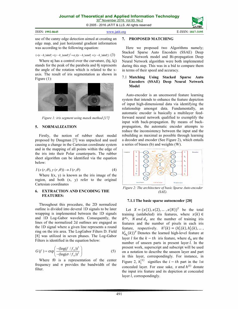
Where αj has a control over the curvature, (hj, kj) stands for the peak of the parabola and θj represents the angle of the rotation which is related to the x-axis. The result of iris segmentation as shown in Figure (1):

Figure 1: iris segment using masek method [17] 5. NORMALIZATION

Firstly, the notion of rubber sheet modal

proposed by Daugman [7] was unpacked and used causing a change in the Cartesian coordinate system and in the mapping of all points within the edge of the iris into their Polar counterparts. The rubber sheet algorithm can be identified via the equation below:

( ( , ), ( , )) ( , )I x r y r I rθ θ θ→ (4)

Where I(x, y) is known as the iris image of the region, and both (x, y) refer to the original Cartesian coordinates

6. EXTRACTION AND ENCODING THE

FEATURES:

Throughout this procedure, the 2D normalized

outline is divided into deveral 1D signals to be later wrapping is implemented between the 1D signals and 1D Log-Gabor wavelets. Consequently, the lines of the normalized 2d outlines are engaged as the 1D signal where a given line represents a round ring on the iris area. The LogGabor Filters D. Field [8] was utilized in seven phases. The Log-Gabor Filters is identified in the equation below:

20

20

(log( / ))( ) exp

(log( / ))

f fG f

fσ

−=

−

(5)

Where f0 is a representation of the center frequency and σ provides the bandwidth of the filter.

7. PROPOSED MATCHING Here we proposed two Algorithms namely;

Stacked Sparse Auto Encoders (SSAE) Deep Neural Network model and Bi-propagation Deep Neural Network algorithm were both implemented during this step. This was in a bid to compare them in terms of their speed and accuracy.

7.1 Matching Using Stacked Sparse Auto

Encoders (SSAE) Deep Neural Network

Model

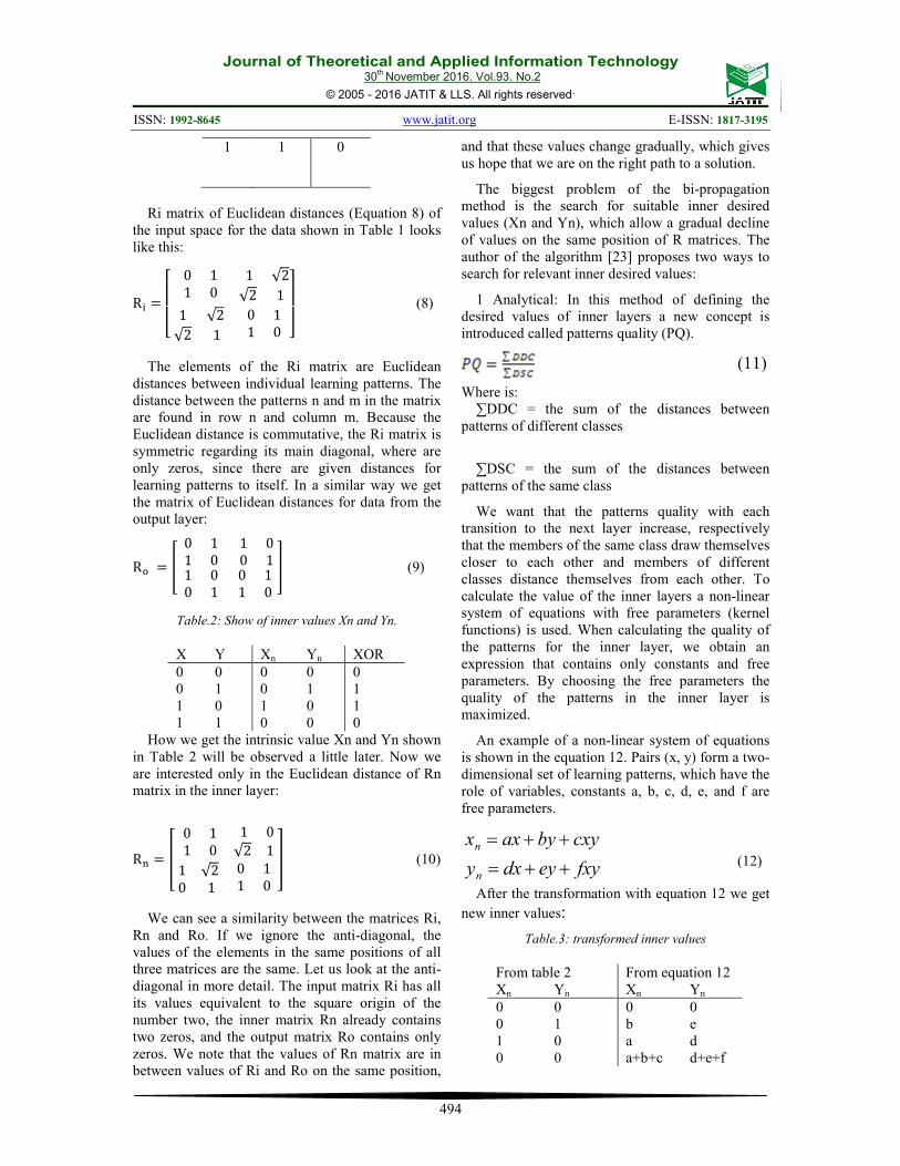
Auto-encoder is an uncensored feature learning system that intends to enhance the feature depiction of input high-dimensional data via identifying the relationship amongst data. Fundamentally, an automatic encoder is basically a multilayer feed-forward neural network qualified to exemplify the input with back-propagation. By means of back-propagation, the automatic encoder attempts to reduce the inconsistency between the input and the rebuilding as maximal as possible through learning a decoder and encoder (See Figure 2), which entails a series of biases (b) and weights (W).

Figure 2: The architecture of basic Sparse Auto-encoder

(SAE).

7.1.1 The basic sparse autoencoder [20]

Let � � ��1�, ��2�, …, �� be the total training (unlabeled) iris features, where �� ∈�� , �� are the number of training iris features and the number of pixels in each iris feature, respectively. �� , �� , … ,�� Denotes the learned high-level feature at

layer � for the � �� iris feature, where �� are the number of unseen parts in present layer�. In the present work, superscript and subscript will be used on a notation to describe the unseen layer and part in this layer, correspondingly. For instance, in

Figure 2, �� signifies the � �� part in the 1st

concealed layer. For ease sake, �� donate the input iris feature and its depiction at concealed layer�, correspondingly.





492

The architecture of basic Sparse Autoencoder (SAE) is illustrated in Figure 2. Overall, the input layer of the automatic encoder contains an encoder that works on the transformation of input � in the parallel demonstration�, and the concealed layer � might be taken as a novel feature demonstration of input data. The output layer is efficiently a decipherer that has been taught to restructure an estimate �! of the input from the concealed illustration�. Essentially, the process of training an automatic encoder is meant to detect optimum parameters via decreasing the inconsistency between input � and its rebuilding�!.

This inconsistency is labelled with a cost function where the cost function of a Sparse Autoencoder (SAE) includes three conditions as follows [3]:

"#$%�θ� � '1N ) *L ,x�k�, d01 2e045x�k�6789:;<� =

>?α ∑ KL�ρ||ρ! E�FE<� G > Hβ‖W‖��L (6)

The first term refers to the average sum-of-squares error, which designates the inconsistency between input �� and reconstruction �!� � over the whole data. Encoder MN4�∙� maps input � ∈ �� to the hidden representation� ∈ �� , which is outlined by� � MN4�� P�Q� > R��, where W is a �� S �� weight matrix and R� ∈ �� is an unfairness route. The encoder is parameterized byTU � �Q, R��. Decoder �N1�∙�maps resultant concealed representation � back into input space�!. �! � �N1 � P�Q�� >R��, where Q� is a �� S �V weight matrix and R� ∈ �� is an unfairness route. Here P�W� is the stimulation function that is outlined

by sigmoid logistic function as P�X� � ��YZ[\ ,

where Xis the pre-activation of a neuron. Therefore, the decoder is parameterized byT � �Q� , R��. The weight matrix Q� of the contrary plotting is the reorder of weight matrixQ. Consequently, the autoencoder is thought to have got tie weights that can successfully decrease the number of the factors of the weight matrix into half. As a result, the pre-activation of the output layers of the auto-encoder may be made in three factors T � �Q, R� , R�� as] � Q�P�Q� > R�� > R�. Thus, the reconstitution �!by decipherer may be calculated as�! � P�]�. Principally, the training an auto-encoder is meant to detect the best factorsT � �Q,R�, R�� concurrently through reducing the reconstruction error defined by the first term. The cost function ^�∙,∙� evaluates the inconsistency

between input � and the reconstruction �! by decoder�N1�∙�.

On the other hand, the second term �� refers to the number of parts in a concealed layer, and the index _ is summing over the concealed parts in the network. `^�a||a!b� Is the Kullback-Leibler (KL) deviation betweena!b, the typical activation (averaged over the training set) of concealed part _, and the required activations ab that is described

asa log ffgh > �1 � a� log �if�ifgh. Moreover, the third term refers to the weight

decline term, which has a tendency to decrease the amount of the weight, and aids the prevention of over fitting. Here

‖W‖�� tr�WlW� � ) ) ) 2wn,E�o�7�pqE

pq[rn

Fqo<�

Where �� denotes the number of layers and P� denotes the number of neurons in the layer�. s�,b��denotes the association between � �� neuron

in layer � � 1 and _ � �� neuron in layer�. For the SAE considered in the present work, the parameters of SAE are �� = 2,P� = 6720, P� = 2000.

7.1.2 Stacked sparse autoencoder (ssae) [20]

The loaded auto-encoder is a neural network

comprising numerous layers of plain SAE where the outputs of a layer is bound to the inputs of the following layer. The present study constructs two layers SSAE that include two plain SAE. The construction of SSAE is illustrated in Figure 3. For ease sake, the study shows the decipherer units of every plain SAE in the figure.

Figure 3: The architecture of Stacked Sparse

Autoencoder (SSAE) and Softmax Classifier for iris

classification

The SSAE is controlled by the function t:�� →��w� that transforms input raw pixels of iris

feature into a novel feature representation�� t�� ∈ ��w� . As for the first layer or the input





493

layer, the input is the raw pixel of iris feature. This input is embodied as a column route of pixel feature with 28 × 240 size. There are ��= 28 × 240 = 6720 input parts in the input layer. Both of the concealed layers have ��r�= 2000 and ��w� = 1000 concealed parts, correspondingly.

7.1.3 Training the SSAE

The construction of SSAE is illustrated in Figure 3. The greedy layer-wise method is employed for pre-training SSAE by training all layers sequentially. After the pre-training, the trained SSAE will be employed to feature iris classification in a testing group.

A SAE is first located on the raw inputs � to identify major features �� on the raw input through regulating the weightQ��.

After that, the raw input is served into this trained sprinkled autoencoder, attaining the major feature activations �� for each of the input iris features�. The major characteristics will be employed as the “raw input” to a new sprinkled autoencoder to detect minor characteristics �� on these major characteristics.

After that, the major characteristics can be served into another SAE to get the minor feature activations ��for each of the major characteristics��, which match up with the major characteristics of the equivalent input iris characteristics�. These minor characteristics are considered as “raw input” to a softmax categorizer, training it to plot minor characteristics to digit tags.

Eventually, the three layers are combined to make a SSAE with 2 concealed layers and a last softmax categorizer layer which is able of categorizing the iris characteristics of MBGC v1 NIR Video database as desired.

7.2 Matching Using BI-Propagation Deep

Neural Network Algorithm

The Bi-propagation algorithm is the intermediary link between the gradient and non-gradient algorithms. It was discovered by Bojan Ploj in 2009 [23] as an improvement of the back-propagation algorithm. Bi-propagation has retained its predecessor's iterativeness and non-constructiveness and took over the idea of kernel functions from the support vectors machine. Kernel function in the first layer makes the partially linearisation of the input space and thus allowing faster and more reliable learning of the subsequent layers. It often happens that due to the difficult learning patterns the back-

propagation method completely fails, while due to linearization the bi-propagation method in the same conditions is fast, efficient and reliable.

The original idea of the Bi-propagation algorithm is that the hidden layers MLP obtain the desired values. Thus, the N-layer perceptron is divided into N single-layer perceptrons and with that the complex problem of learning is divided into several simpler problems, independent of each other. Learning thus becomes easier, faster and more reliable than the back-propagation method. The prefix bi- in the name of the algorithm arose because the corrections of weights synapses during learning spread in both directions (forward and backward).

The gradualness of the bi-propagation method from layer to layer is also evident in the matrix of Euclidean distances between learning patterns (Equation 8). The elements on the same position of the matrix from the input layer towards the output gradually change the values (equation 8, 9 and 10).

7.2.1 Description of the Bi-propagation

algorithm

We will describe the algorithm with the logical

XOR function example. As already stated, the main concept of the bi-propagation algorithm is that the inner layers are no longer hidden, but get the desired output values. With this measure learning of the entire MLP is divided into learning of two individual, linear layers which has no problem with local minima.

Suitable MLP construction for this problem is shown in Figure 4. The XOR function was chosen for this example because it is not extensive and also contains local minima, which causes problems to many other methods.

Figure 4: Multi-layer perceptron, which successfully

solves the XOR problem.

Table.1: Logical XOR function.

X y XOR 0 0 1

0 1 0

0 1 1

Y X

Xn Yn

XOR





494

1 1 0

Ri matrix of Euclidean distances (Equation 8) of

the input space for the data shown in Table 1 looks like this:

Rn � yzzz{ 0 11 0 1 √2√2 11 √2√2 1 0 11 0 ~��

�� (8)

The elements of the Ri matrix are Euclidean

distances between individual learning patterns. The distance between the patterns n and m in the matrix are found in row n and column m. Because the Euclidean distance is commutative, the Ri matrix is symmetric regarding its main diagonal, where are only zeros, since there are given distances for learning patterns to itself. In a similar way we get the matrix of Euclidean distances for data from the output layer:

R� � �0 11 0 1 00 11 00 1 0 11 0� (9)

Table.2: Show of inner values Xn and Yn.

X Y Xn Yn XOR 0 0 1 1

0 1 0 1

0 0 1 0

0 1 0 0

0 1 1 0

How we get the intrinsic value Xn and Yn shown in Table 2 will be observed a little later. Now we are interested only in the Euclidean distance of Rn matrix in the inner layer:

RF � �0 11 0 1 0√2 11 √20 1 0 11 0 � (10)

We can see a similarity between the matrices Ri,

Rn and Ro. If we ignore the anti-diagonal, the values of the elements in the same positions of all three matrices are the same. Let us look at the anti-diagonal in more detail. The input matrix Ri has all its values equivalent to the square origin of the number two, the inner matrix Rn already contains two zeros, and the output matrix Ro contains only zeros. We note that the values of Rn matrix are in between values of Ri and Ro on the same position,

and that these values change gradually, which gives us hope that we are on the right path to a solution.

The biggest problem of the bi-propagation method is the search for suitable inner desired values (Xn and Yn), which allow a gradual decline of values on the same position of R matrices. The author of the algorithm [23] proposes two ways to search for relevant inner desired values:

1 Analytical: In this method of defining the desired values of inner layers a new concept is introduced called patterns quality (PQ).

(11)

Where is: ∑DDC = the sum of the distances between

patterns of different classes

∑DSC = the sum of the distances between

patterns of the same class

We want that the patterns quality with each transition to the next layer increase, respectively that the members of the same class draw themselves closer to each other and members of different classes distance themselves from each other. To calculate the value of the inner layers a non-linear system of equations with free parameters (kernel functions) is used. When calculating the quality of the patterns for the inner layer, we obtain an expression that contains only constants and free parameters. By choosing the free parameters the quality of the patterns in the inner layer is maximized.

An example of a non-linear system of equations is shown in the equation 12. Pairs (x, y) form a two-dimensional set of learning patterns, which have the role of variables, constants a, b, c, d, e, and f are free parameters.

fxyeydxy

cxybyaxx

n

n

++=

++= (12)

After the transformation with equation 12 we get

new inner values:

Table.3: transformed inner values

From table 2 From equation 12 Xn Yn Xn Yn 0 0 1 0

0 1 0 0

0 b a a+b+c

0 e d d+e+f





495

From that the free parameters can easily be calculated:

a = 1, b = 0, c = -1, d = 0, e = 1, f = -1 (13)

By inserting them in the non-linear system of equations we get:

xyyxy

xyyxx

n

n

110

101

−+=

−+= (14)

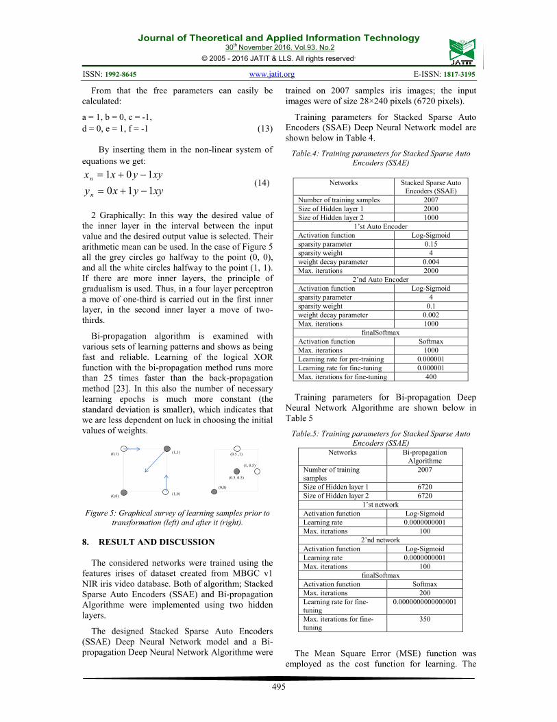
2 Graphically: In this way the desired value of

the inner layer in the interval between the input value and the desired output value is selected. Their arithmetic mean can be used. In the case of Figure 5 all the grey circles go halfway to the point (0, 0), and all the white circles halfway to the point (1, 1). If there are more inner layers, the principle of gradualism is used. Thus, in a four layer perceptron a move of one-third is carried out in the first inner layer, in the second inner layer a move of two-thirds.

Bi-propagation algorithm is examined with various sets of learning patterns and shows as being fast and reliable. Learning of the logical XOR function with the bi-propagation method runs more than 25 times faster than the back-propagation method [23]. In this also the number of necessary learning epochs is much more constant (the standard deviation is smaller), which indicates that we are less dependent on luck in choosing the initial values of weights.

Figure 5: Graphical survey of learning samples prior to

transformation (left) and after it (right).

8. RESULT AND DISCUSSION

The considered networks were trained using the

features irises of dataset created from MBGC v1 NIR iris video database. Both of algorithm; Stacked Sparse Auto Encoders (SSAE) and Bi-propagation Algorithme were implemented using two hidden layers.

The designed Stacked Sparse Auto Encoders (SSAE) Deep Neural Network model and a Bi-propagation Deep Neural Network Algorithme were

trained on 2007 samples iris images; the input images were of size 28×240 pixels (6720 pixels).

Training parameters for Stacked Sparse Auto Encoders (SSAE) Deep Neural Network model are shown below in Table 4.

Table.4: Training parameters for Stacked Sparse Auto

Encoders (SSAE)

Networks Stacked Sparse Auto

Encoders (SSAE) Number of training samples 2007 Size of Hidden layer 1 2000 Size of Hidden layer 2 1000

1’st Auto Encoder Activation function Log-Sigmoid sparsity parameter 0.15 sparsity weight 4 weight decay parameter 0.004 Max. iterations 2000

2’nd Auto Encoder Activation function Log-Sigmoid sparsity parameter 4 sparsity weight 0.1 weight decay parameter 0.002 Max. iterations 1000

finalSoftmax Activation function Softmax Max. iterations 1000 Learning rate for pre-training 0.000001 Learning rate for fine-tuning 0.000001 Max. iterations for fine-tuning 400

Training parameters for Bi-propagation Deep

Neural Network Algorithme are shown below in Table 5

Table.5: Training parameters for Stacked Sparse Auto

Encoders (SSAE) Networks Bi-propagation

Algorithme Number of training samples

2007

Size of Hidden layer 1 6720 Size of Hidden layer 2 6720

1’st network Activation function Log-Sigmoid Learning rate 0.0000000001 Max. iterations 100

2’nd network Activation function Log-Sigmoid Learning rate 0.0000000001 Max. iterations 100

finalSoftmax Activation function Softmax Max. iterations 200 Learning rate for fine-tuning

0.0000000000000001

Max. iterations for fine-tuning

350

The Mean Square Error (MSE) function was employed as the cost function for learning. The

(0,0)

(0,1)

(1,0)

(1,1)

(0,0)

(0.5 ,1)

(1, 0.5)

(0.5, 0.5)





496

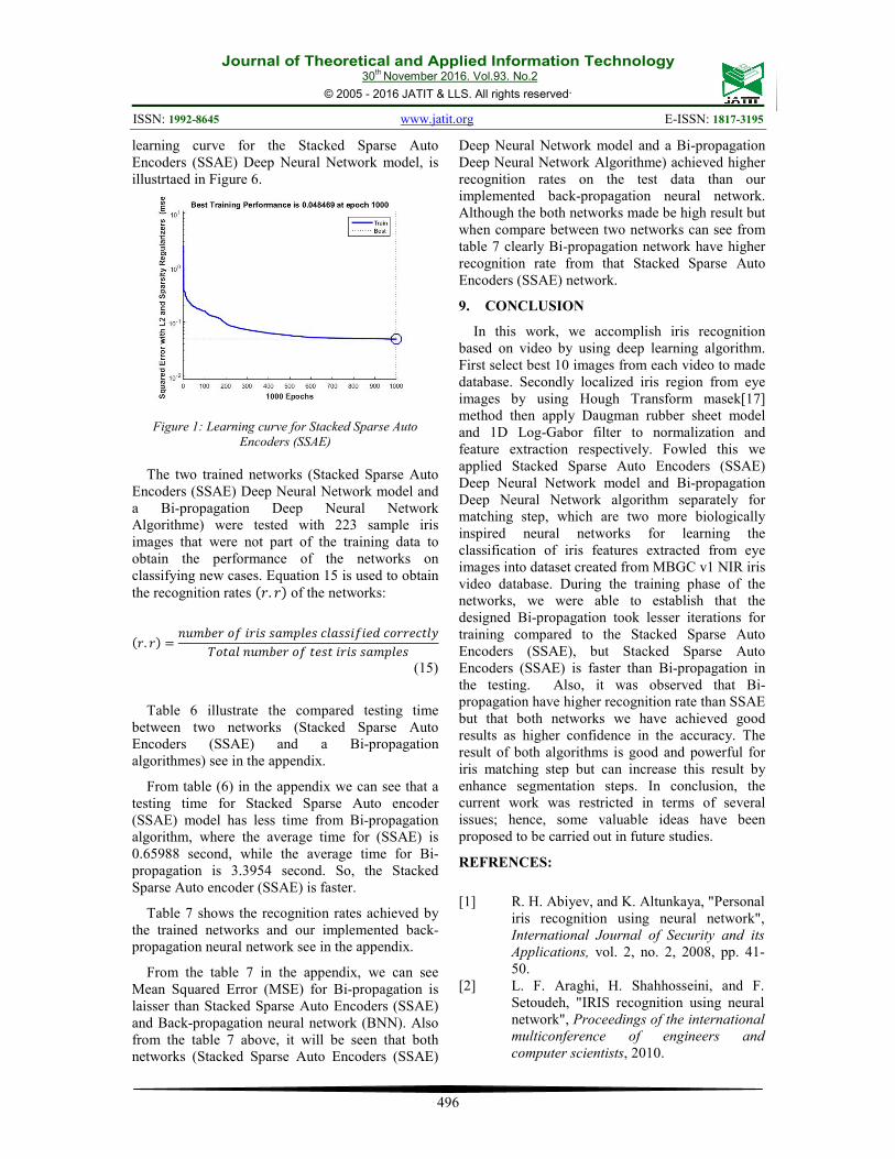
learning curve for the Stacked Sparse Auto Encoders (SSAE) Deep Neural Network model, is illustrtaed in Figure 6.

Figure 1: Learning curve for Stacked Sparse Auto

Encoders (SSAE)

The two trained networks (Stacked Sparse Auto Encoders (SSAE) Deep Neural Network model and a Bi-propagation Deep Neural Network Algorithme) were tested with 223 sample iris images that were not part of the training data to obtain the performance of the networks on classifying new cases. Equation 15 is used to obtain the recognition rates ��. �� of the networks:

��. �� RM��t � PP��MP��PP t M��M��]��RM��t�MP� � PP��MP

(15)

Table 6 illustrate the compared testing time between two networks (Stacked Sparse Auto Encoders (SSAE) and a Bi-propagation algorithmes) see in the appendix.

From table (6) in the appendix we can see that a testing time for Stacked Sparse Auto encoder (SSAE) model has less time from Bi-propagation algorithm, where the average time for (SSAE) is 0.65988 second, while the average time for Bi-propagation is 3.3954 second. So, the Stacked Sparse Auto encoder (SSAE) is faster.

Table 7 shows the recognition rates achieved by the trained networks and our implemented back-propagation neural network see in the appendix.

From the table 7 in the appendix, we can see Mean Squared Error (MSE) for Bi-propagation is laisser than Stacked Sparse Auto Encoders (SSAE) and Back-propagation neural network (BNN). Also from the table 7 above, it will be seen that both networks (Stacked Sparse Auto Encoders (SSAE)

Deep Neural Network model and a Bi-propagation Deep Neural Network Algorithme) achieved higher recognition rates on the test data than our implemented back-propagation neural network. Although the both networks made be high result but when compare between two networks can see from table 7 clearly Bi-propagation network have higher recognition rate from that Stacked Sparse Auto Encoders (SSAE) network.

9. CONCLUSION

In this work, we accomplish iris recognition based on video by using deep learning algorithm. First select best 10 images from each video to made database. Secondly localized iris region from eye images by using Hough Transform masek[17] method then apply Daugman rubber sheet model and 1D Log-Gabor filter to normalization and feature extraction respectively. Fowled this we applied Stacked Sparse Auto Encoders (SSAE) Deep Neural Network model and Bi-propagation Deep Neural Network algorithm separately for matching step, which are two more biologically inspired neural networks for learning the classification of iris features extracted from eye images into dataset created from MBGC v1 NIR iris video database. During the training phase of the networks, we were able to establish that the designed Bi-propagation took lesser iterations for training compared to the Stacked Sparse Auto Encoders (SSAE), but Stacked Sparse Auto Encoders (SSAE) is faster than Bi-propagation in the testing. Also, it was observed that Bi-propagation have higher recognition rate than SSAE but that both networks we have achieved good results as higher confidence in the accuracy. The result of both algorithms is good and powerful for iris matching step but can increase this result by enhance segmentation steps. In conclusion, the current work was restricted in terms of several issues; hence, some valuable ideas have been proposed to be carried out in future studies.

REFRENCES:

[1] R. H. Abiyev, and K. Altunkaya, "Personal iris recognition using neural network", International Journal of Security and its

Applications, vol. 2, no. 2, 2008, pp. 41-50.

[2] L. F. Araghi, H. Shahhosseini, and F. Setoudeh, "IRIS recognition using neural network", Proceedings of the international

multiconference of engineers and

computer scientists, 2010.





497

[3] Y. Bengio, A. Courville, and P. Vincent, "Representation learning: A review and new perspectives", IEEE transactions on

pattern analysis and machine intelligence, vol. 35, no. 8, 2013, pp. 1798-1828.

[4] W. W. Boles, and B. Boashash, "A human identification technique using images of the iris and wavelet transform", IEEE

transactions on signal processing, vol. 46, no. 4, 1998, pp. 1185-1188.

[5] C. Candemir, C. Çetinkaya, O. Kılınççeker et al., "Vascular landmark classification in retinal images using fuzzy RBF", Signal

Processing and Communications

Applications Conference (SIU), 2013 21st, 2013, pp. 1-4.

[6] Chaudhary U. and Mubarak C. M., "Iris Recognition Using BPNN Algorithm", International Journal of Engineering

Research and Applications (IJERA),, vol., no. 2248-9622 National Conference on Emerging Trends in Engineering & Technology, , 2012.

[7] J. G. Daugman, "High confidence visual recognition of persons by a test of statistical independence", IEEE

transactions on pattern analysis and

machine intelligence, vol. 15, no. 11, 1993, pp. 1148-1161.

[8] D. J. Field, "Relations between the statistics of natural images and the response properties of cortical cells", JOSA A, vol. 4, no. 12, 1987, pp. 2379-2394.

[9] S. Godara, and R. Gupta, "Neural Networks for Iris Recognition: Comparisons between LVQ and Cascade Forward Back Propagation Neural network Models, Architectures and Algorithm", Neural Networks, vol. 3, no. 1, 2013.

[10] M. Gopikrishnan, and D. T. Santhanam, "A tradeoff between template size reduction and computational accuracy in Iris Patterns Recognition using Neural Networks", seec proceedings by, SEEC, vol., no., 2010.

[11] M. Gopikrishnan, and T. Santhanam, "Effect of different neural networks on the accuracy in iris patterns recognition", International Journal of Reviews in

computing, vol. 7, no., 2011, pp. 22-28. [12] M. Gopikrishnan, and T. Santhanam,

"Effect of Training Algorithms on the Accuracy in Iris Patterns Recognition using Neural Networks", International

Journal of Computer Science and

Telecommunications, vol. 2, no. 7, 2011. [13] A. E. Hassanien, A. Abraham, and C.

Grosan, "Spiking neural network and wavelets for hiding iris data in digital images", Soft Computing, vol. 13, no. 4, 2009, pp. 401-416.

[14] F. S. Helmli, and S. Scherer, "Adaptive shape from focus with an error estimation in light microscopy", Image and Signal

Processing and Analysis, 2001. ISPA

2001. Proceedings of the 2nd International

Symposium on, 2001, pp. 188-193. [15] S. Lim, K. Lee, O. Byeon et al., "Efficient

iris recognition through improvement of feature vector and classifier", ETRI

journal, vol. 23, no. 2, 2001, pp. 61-70. [16] L. Ma, Y. Wang, and T. Tan, "Iris

recognition using circular symmetric filters", Pattern Recognition, 2002.

Proceedings. 16th International

Conference on, 2002, pp. 414-417. [17] L. Masek, "Recognition of human iris

patterns for biometric identification", The

University of Western Australia, vol. 2, no., 2003.

[18] J. R. Matey, O. Naroditsky, K. Hanna et

al., "Iris on the move: Acquisition of images for iris recognition in less constrained environments", Proceedings of

the IEEE, vol. 94, no. 11, 2006, pp. 1936-1947.

[19] A. Murugan, and G. Savithiri, "Fragmented iris recognition system using BPNN", International Journal of

Computer Applications, vol. 36, no. 4, 2011, pp. 28-33.

[20] A. Ng, "Sparse autoencoder", CS294A

Lecture notes, vol. 72, no., 2011, pp. 1-19. [21] A. Peter, N. Revathi, and A. P. M. M.

Mercy, "Neural network based Matching approach for Iris recognition", International Journal of Advanced

Research in Computer Engineering &

Technology (IJARCET), vol. 2, no. 2, 2013, pp. pp: 618-623.

[22] P. J. Phillips, P. J. Flynn, J. R. Beveridge

et al., "Overview of the multiple biometrics grand challenge", International

Conference on Biometrics, 2009, pp. 705-714.

[23] B. Ploj, "Bipropagation-nov način učenja večslojnega perceptrona (MLP)", vol., no., 2009.





498

[24] C. M. M. Prof Ujval Chaudhary "IRIS RECOGNITION USING BPNN ALGORITHM", International Journal of

Engineering Research and Applications

(IJERA), vol., no., pp. 203-208. [25] K. A. Raghavi, M. V. Priya, G. P. M.

Paiva et al., "Human iris recognition using fuzzy neural concepts", The International

Conference on Bioscience, Biochemistry

and Bioinformatics (IPCBEE), 2011, pp. 256-260.

[26] K. Saminathan, M. C. Devi, and T. Chakravarthy, "Pair of Iris Recognition for Personal Identification Using Artificial Neural Network", IJCSI International

Journal of Computer Science, vol., no., 2012.

[27] D. Sánchez, P. Melin, O. Castillo et al., "Modular granular neural networks optimization with multi-objective hierarchical genetic algorithm for human recognition based on iris biometric", 2013

IEEE Congress on Evolutionary

Computation, 2013, pp. 772-778. [28] M. Shams, M. Rashad, O. Nomir et al.,

"Iris recognition based on LBP and combined LVQ classifier", arXiv preprint

arXiv:1111.1562, vol., no., 2011. [29] Sherline Jesie R., "Multimodel

Authentication System using Artificial Neural Network", International Conf. on

Emerging Technology Trends (ICETT),

Proceedings published by International

Journal of Computer Applications (IJCA), vol., no., 2011.

[30] Ö. F. Söylemez, and B. Ergen, "Circular hough transform based eye state detection in human face images", Signal Processing

and Communications Applications

Conference (SIU), 2013 21st, 2013, pp. 1-4.

[31] R. P. Wildes, "Iris recognition: an emerging biometric technology", Proceedings of the IEEE, vol. 85, no. 9, 1997, pp. 1348-1363.

[32] R. P. Wildes, J. C. Asmuth, G. L. Green et

al., "A system for automated iris recognition", Applications of Computer

Vision, 1994., Proceedings of the Second

IEEE Workshop on, 1994, pp. 121-128.





499

Table 6: Testing Time

Number of Images

Name of Images

Testing Time for Stacked Sparse Auto encoder(SSAE)

Testing Time for Bi-propagation

1 S1003L02 0.6445 3.3131 2 S1009R03 0.6484 3.3917 3 S1010L01 0.6493 3.4097 4 S1010L09 0.6575 3.3745 5 S1010R01 0.6645 3.4242 6 S1010R08 0.6594 3.4023 7 S1011L05 0.6596 3.3902 8 S1011L07 0.6683 3.4247 9 S1011R01 0.6677 3.4593

10 S1011R03 0.6613 3.4409 11 S1011R04 0.6539 3.4106 12 S1014L02 0.6502 3.3753 13 S1014L08 0.6606 3.4129 14 S1015R01 0.6621 3.4025 15 S1025L06 0.663 3.3954 16 S1026R07 0.6629 3.4518 17 S1042L02 0.6636 3.3997 18 S1053R01 0.6537 3.3666 19 S1053R04 0.6593 3.38 20 S1060L02 0.6644 3.3615 21 S1060L08 0.6576 3.3883 22 S1065R01 0.6631 3.4049 23 S1065R08 0.6696 3.3819 24 S1067R01 0.6664 3.3731 25 S1068L01 0.6468 3.3994 26 S1068L05 0.6624 3.3732 27 S1074L06 0.6617 3.3842 28 S1093R01 0.6743 3.4115 29 S1099L01 0.6592 3.3627 30 S1106L03 0.6611 3.3985

Average Time 0.65988 3.3954

From table (6) above we can see that a testing time for Stacked Sparse Auto encoder (SSAE) model has less time from Bi-propagation algorithm, where the average time for (SSAE) is 0.65988 second, while the average time for Bi-propagation is 3.3954 second. So, the Stacked Sparse Auto encoder (SSAE) is faster.

Table 7: Testing of Networks.

Network Stacked Sparse Auto Encoders (SSAE)

Bi-propagation Back-propagation neural network (BNN)

Number of test iris samples 223 223 223 Mean Squared Error (MSE) 0.0017 0.0014 0.0427

Correctly classified iris samples

213 216 152

Recognition rate 95.5157% 96.86098% 68.1614%

Documents

DEEP NEURAL NETWORKS FOR IRIS … of iris recognition that can overcomes the restrictions of individual’s identification approaches. They employed a quick algorithm for