Deep Learning Theory and PracticeLecture 15

Recurrent Neural Networks

Dr. Ted Willke willke@pdx.edu

Tuesday, February 25, 2020

Review of Lecture 14• GoogLeNet’s Inception module

2

- Multiple filter sizes in one module

- Dimensionality reduction to reduce ops

Review of Lecture 14

3

• Full GoogLeNet architecture- Eliminated expensive FC layers for classification- Global Average Pooling

- Used auxiliary classification units to inject gradient- Better choice: Batch Normalization

(a batch of activations)

(desired transform)

(Ioffe and Szegedy 2015)Let model learn the best distribution!(not forced to have mean 0, var of 1, but still standardized)

Review of Lecture 14

4

- Implementing Batch Norm in PyTorch

- Fit a residual mapping to combat optimization issues

- Also added “bottleneck” layers for dimensionality reduction

- By convention, normalize the signal at neural input.

• ResNet: Residual connections, deep networks

Review of Lecture 14

5

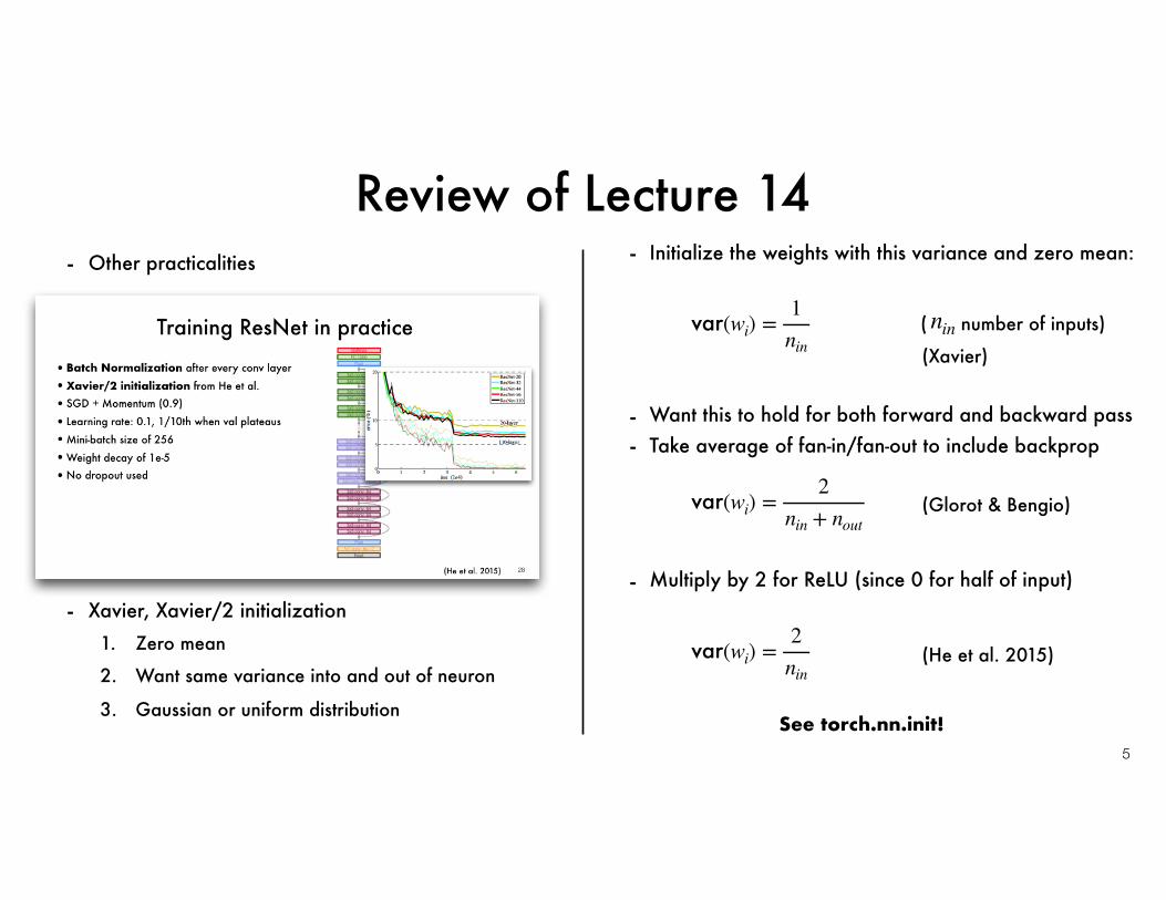
- Other practicalities

- Want this to hold for both forward and backward pass

- Xavier, Xavier/2 initialization1. Zero mean

2. Want same variance into and out of neuron

3. Gaussian or uniform distribution

( number of inputs)

(Xavier)

var(wi) =1

nin

- Initialize the weights with this variance and zero mean:

nin

- Take average of fan-in/fan-out to include backprop

var(wi) =2

nin + nout(Glorot & Bengio)

- Multiply by 2 for ReLU (since 0 for half of input)

var(wi) =2

nin(He et al. 2015)

See torch.nn.init!

Review of Lecture 14

6

• Rapid advancement in accuracy and efficiency • Work needed on processing rates and power

Review of Lecture 14

7

Many other notable architectures and advancements…

•Network in Network: Influenced both GoogLeNet and ResNet

•More general use of “identity mappings” from ResNet

•Wider and aggregated networks

•Networks with stochastic depth

•Fractal networks

•Densely connected convolutional networks

•Efficient networks (compression)

… to name a few!

Today’s Lecture

•Introduction to recurrent neural networks

8(Many slides adapted from Stanford’s excellent CS231n course. Thank you Fei-Fei Li, Justin Johnson, and Serena Young!)

Feedforward neural networks

9

One input

One output

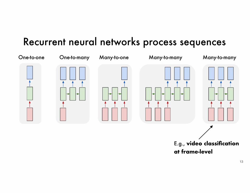
Recurrent neural networks process sequences

10

One-to-one One-to-many

E.g., image captioning Image to sequence of words

Recurrent neural networks process sequences

11

One-to-one One-to-many Many-to-one

E.g., sentiment classification Sequence of words to sentiment

Recurrent neural networks process sequences

12

One-to-one One-to-many Many-to-one Many-to-many

E.g., machine translation sequence of words tosequence of words

Recurrent neural networks process sequences

13

One-to-one One-to-many Many-to-one Many-to-many Many-to-many

E.g., video classification at frame-level

Sequential processing of non-sequential data

14

Classify images by “sequential spatial attention”

(Gregor et al., “DRAW: A Recurrent Neural Network For Image Generation”, ICML 2015)

Sequential processing of non-sequential data

15

Generate images one portion at a time!

(Gregor et al., “DRAW: A Recurrent Neural Network For Image Generation”, ICML 2015)

Recurrent neural network

16

Want to predict a vectorat time steps

Recurrent neural network

17

Can process a sequence of vectors by applyinga recurrence formula at each time step:

xt

ht = fW(ht−1, xt)

new state some function with params, W

old state input vector at time t

The same function and parameters are used at every time step!

A “plain” recurrent neural network

18

ht = fW(ht−1, xt)

The state consists of a single “hidden” vector :h

yt = Whyht

ht = tanh (Whhht−1 + Wxhxt)

The RNN computation graph

19

Recurrent feedback can be ‘unrolled’ into a computation graph.

The RNN computation graph

20

Recurrent feedback can be ‘unrolled’ into a computation graph.

The RNN computation graph

21

Recurrent feedback can be ‘unrolled’ into a computation graph.

The RNN computation graph

22

Reuse the same weight matrix at each time step!

When thinking about backprop, separate gradient will flow back for each time step.

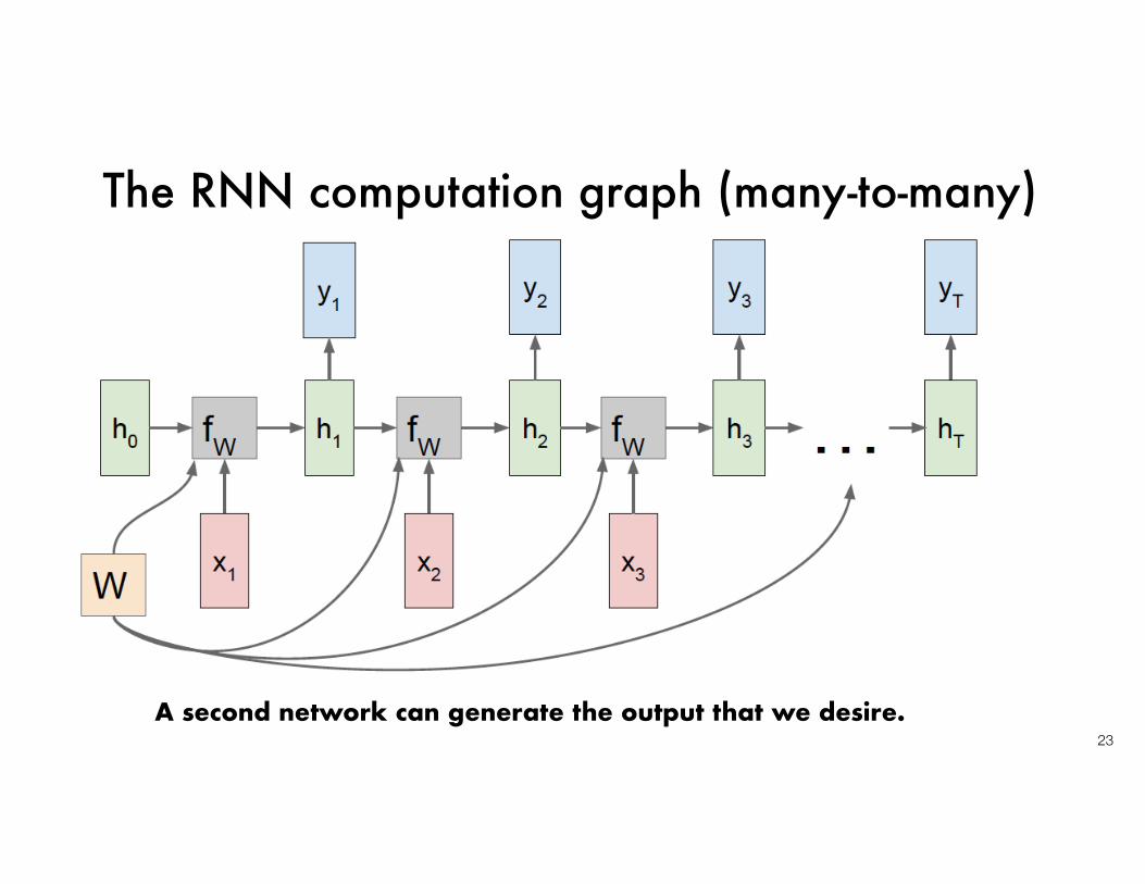
The RNN computation graph (many-to-many)

23A second network can generate the output that we desire.

The RNN computation graph (many-to-many)

24Can compute an individual loss at every time step as well (e.g., softmax loss of labels)

The RNN computation graph (many-to-many)

25Total loss for entire training step is sum of losses (compute gradient of loss w.r.t. W)

The RNN computation graph (many-to-one)

26Final hidden state summarizes all context (can best predict, e.g., sentiment)

The RNN computation graph (one-to-many)

27Fixed size input, variably sized output (e.g., image captioning)

y1 y2

Sequence-to-sequence

28

Many-to-one: Encode input sequence into single vector…

Variably-sized input and output (e.g., machine translation)

One-to-many: Decode output sequencefrom single input vector….

Example: Character-level language model

29

Predicting the next character…

Vocabulary: [h,e,l,o]

Training sequence: “hello”

Example: Character-level language model

30

Predicting the next character…

Vocabulary: [h,e,l,o]

Training sequence: “hello”

ht = tanh (Whhht−1 + Wxhxt)

Example: Character-level language model

31

Predicting the next character…

Vocabulary: [h,e,l,o]

Training sequence: “hello”

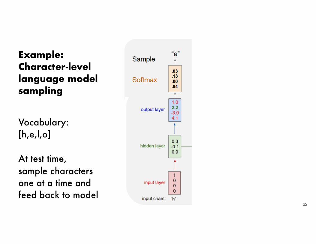
Example: Character-level language modelsampling

32

Vocabulary: [h,e,l,o]

At test time, sample charactersone at a time andfeed back to model

Example: Character-level language modelsampling

33

Vocabulary: [h,e,l,o]

At test time, sample charactersone at a time andfeed back to model

Example: Character-level language modelsampling

34

Vocabulary: [h,e,l,o]

At test time, sample charactersone at a time andfeed back to model

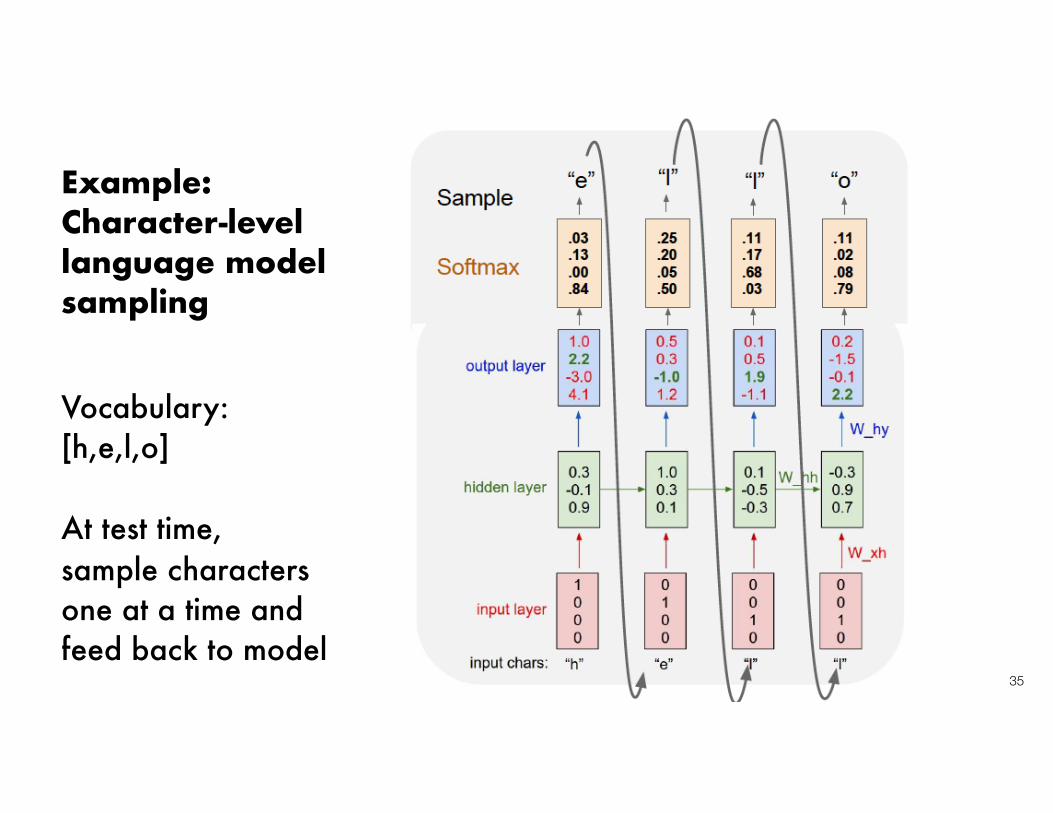
Example: Character-level language modelsampling

35

Vocabulary: [h,e,l,o]

At test time, sample charactersone at a time andfeed back to model

36

Backpropagation through timeRun forward through entire sequence to compute loss, then backwardthrough entire sequence to compute gradient.

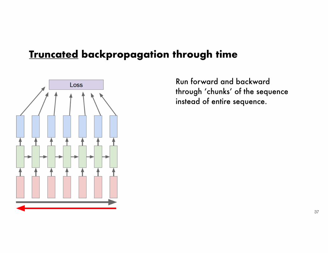
37

Truncated backpropagation through time

Run forward and backwardthrough ‘chunks’ of the sequence instead of entire sequence.

38

Truncated backpropagation through time

Carry hidden states forward in time forever, but only backpropagate for some smaller number of steps.

39

Truncated backpropagation through time

Further reading

• Zhang, A., Lipton, Z. C., Li, M., and Smola, A. J. (2020) Dive into Deep Learning, Release 0.7.1. https://d2l.ai/

• Stanford CS231n Convolutional Neural Networks for Visual Recognition. http://cs231n.github.io/

• Abu-Mostafa, Y. S., Magdon-Ismail, M., Lin, H.-T. (2012) Learning from data. AMLbook.com.

• Goodfellow et al. (2016) Deep Learning. https://www.deeplearningbook.org/

• Boyd, S., and Vandenberghe, L. (2018) Introduction to Applied Linear Algebra - Vectors, Matrices, and Least Squares. http://vmls-book.stanford.edu/

• VanderPlas, J. (2016) Python Data Science Handbook. https://jakevdp.github.io/PythonDataScienceHandbook/

40