Deep Learning Techniques for Cell Stage Classification

Rafael José Costa Freitas

Thesis to obtain the Master of Science Degree in

Aerospace Engineering

Supervisor(s): Prof. Luis CustódioProf. João Sanches

Examination Committee

Chairperson: Prof. Jose Fernando Alves da SilvaSupervisor: Prof. Jõao Sanches

Member of the Committee: Prof. Margarida Silveira

October 2020

ii

Dedicated to my friends and family who never allowed me to forget I was still not a master...

iii

iv

Acknowledgments

First, I would like to thank my thesis supervisors, Luis Custodio and Joao Sanches, for all their help

and support. While it became a long journey to finalize this master thesis, their support and valuable

counseling definitely provided me with all I needed to perform this work.

Next, I would like to thank my family, their unconditional support and love has encouraged me along

my entire journey as a student and has shaped me into the person I am today. You are always there for

me and there is no possible way I could thank you enough. I would also like to take this opportunity to

apologize for all headaches and concerns I caused along the years, even though I cannot promise I will

not do it again.

Next there are my friends. You have helped me every step of the way, from working on the various

projects we had through college, to always giving me valuable advice or to, probably most important of

all, providing me with the required fun moments and memories to really appreciate these years.

v

vi

Resumo

O ciclo celular corresponde aos varios processos e mecanismos que ocorrem durante as diversas

fases da vida de uma celula e a progressao correta ao longo do mesmo e essencial para a manutencao

da vida.

Para uma celula eucariotica tıpica, este ciclo pode ser separado em 2 fases principais: a interfase,

durante a qual a celula esta em crescimento, e a mitose, onde a celula se separa em duas celulas

filhas. A interfase pode ainda ser dividida em 3 fases principais, G1, onde a celula esta em fase de

crescimento, a fase S, onde o DNA celular e replicado e a fase G2, durante a qual a celula continua a

preparacao para a mitose.

Devido a importancia do ciclo celular, a classificacao correta da fase celular e essencial para a

pesquisa biologica e farmacologica. Porem, os metodos atuais de classificacao celular baseiam-se

tradicionalmente na microscopia fluorescente e em analises populacionais. Assim sendo, estes metodos

apresentam algumas desvantagens, como a necessidade de marcadores biologicos especıficos ou a

destruicao da cultura celular para determinar a fase celular.

Como tal, neste projecto e proposto um novo metodo que se baseia no uso de culturas de celulas

marcadas com o composto DAPI (uma das tecnicas de microscopia fluorescente mais comuns) e

tecnicas de deep learning. Utilizando algoritmos de deep learning, este metodo e capaz de classi-

ficar celulas isoladamente sem depender de analises populacionais e sem necessitar de marcadores

biologicos especıficos, resultando num processo bastante mais simples para classificar a fase celular.

Palavras-chave: Deep Learning, Composto DAPI, Microscopia Fluorescente, Ciclo Celular,

Rede Neuronal Convolucional

vii

viii

Abstract

The various phases and mechanisms that happen sequentially during a life of a cell form the cell

cycle and the correct progression along this cycle is essential for the maintenance of life.

For a typical eukaryotes cell this cycle can be separated into 2 main phases: interphase, during

which the cell is growing, and mitosis, where the cell separates into two daughter cells. The interphase

can be further divided into 3 main phases, G1, where the cell is growing, the S phase, where the DNA

is replicated and the G2 phase during which the cell continues growing in preparation for mitosis.

Due to the importance of the cellular cycle, the correct staging of a cell (i.e. correct classification of

its current phase) is of the utmost importance for biological and pharmacological research. However,

current methods for cell staging have traditionally relied on fluorescence microscopy and the analysis

of cell population and present some drawbacks such as the need for specific biological markers or the

destruction of the cell culture to determine its stage.

As such, in this project, a new method that relies on the use of DAPI stained cell cultures (one

of the most common cell imaging techniques) and deep learning techniques is proposed. By using

deep learning algorithms, this method is capable of classifying single data points without relying on cell

population analysis and will not require specific biological markers, resulting in fairly simpler process to

achieve cell staging.

Keywords: Deep learning, DAPI staining, Fluorescent Microscopy, Cell Cycle, Convolutional

Neural Network

ix

x

Contents

Acknowledgments . . . . . . . . . . . . . . . . . . . . . . . . . . . . . . . . . . . . . . . . . . . v

Resumo . . . . . . . . . . . . . . . . . . . . . . . . . . . . . . . . . . . . . . . . . . . . . . . . . vii

Abstract . . . . . . . . . . . . . . . . . . . . . . . . . . . . . . . . . . . . . . . . . . . . . . . . . ix

List of Tables . . . . . . . . . . . . . . . . . . . . . . . . . . . . . . . . . . . . . . . . . . . . . . xiii

List of Figures . . . . . . . . . . . . . . . . . . . . . . . . . . . . . . . . . . . . . . . . . . . . . xv

Glossary . . . . . . . . . . . . . . . . . . . . . . . . . . . . . . . . . . . . . . . . . . . . . . . . xvii

1 Introduction 1

1.1 Motivation . . . . . . . . . . . . . . . . . . . . . . . . . . . . . . . . . . . . . . . . . . . . . 1

1.2 Objectives . . . . . . . . . . . . . . . . . . . . . . . . . . . . . . . . . . . . . . . . . . . . . 2

1.3 Thesis Outline . . . . . . . . . . . . . . . . . . . . . . . . . . . . . . . . . . . . . . . . . . 2

2 Theoretical Background 3

2.1 Biological Background . . . . . . . . . . . . . . . . . . . . . . . . . . . . . . . . . . . . . . 3

2.1.1 The Cell . . . . . . . . . . . . . . . . . . . . . . . . . . . . . . . . . . . . . . . . . . 3

2.1.2 The Cell Cycle . . . . . . . . . . . . . . . . . . . . . . . . . . . . . . . . . . . . . . 4

2.1.3 Cell Imaging . . . . . . . . . . . . . . . . . . . . . . . . . . . . . . . . . . . . . . . 9

2.1.4 Current cell staging techniques . . . . . . . . . . . . . . . . . . . . . . . . . . . . . 11

2.2 Machine Learning . . . . . . . . . . . . . . . . . . . . . . . . . . . . . . . . . . . . . . . . 12

2.2.1 Deep Learning . . . . . . . . . . . . . . . . . . . . . . . . . . . . . . . . . . . . . . 13

3 Methodology 21

3.1 Biological Material and Data . . . . . . . . . . . . . . . . . . . . . . . . . . . . . . . . . . . 21

3.1.1 Cell culture and imaging . . . . . . . . . . . . . . . . . . . . . . . . . . . . . . . . . 21

3.1.2 Image Pipeline . . . . . . . . . . . . . . . . . . . . . . . . . . . . . . . . . . . . . . 22

3.2 Methods . . . . . . . . . . . . . . . . . . . . . . . . . . . . . . . . . . . . . . . . . . . . . . 24

3.2.1 Machine Learning . . . . . . . . . . . . . . . . . . . . . . . . . . . . . . . . . . . . 24

3.3 Validation . . . . . . . . . . . . . . . . . . . . . . . . . . . . . . . . . . . . . . . . . . . . . 29

3.3.1 MNIST dataset . . . . . . . . . . . . . . . . . . . . . . . . . . . . . . . . . . . . . . 29

3.3.2 VGG Network . . . . . . . . . . . . . . . . . . . . . . . . . . . . . . . . . . . . . . . 30

xi

4 Results 31

4.1 Artificial Neural Network . . . . . . . . . . . . . . . . . . . . . . . . . . . . . . . . . . . . . 31

4.2 Convolutional Neural Network . . . . . . . . . . . . . . . . . . . . . . . . . . . . . . . . . . 32

5 Conclusions 35

5.1 Achievements . . . . . . . . . . . . . . . . . . . . . . . . . . . . . . . . . . . . . . . . . . . 35

5.2 Future Work . . . . . . . . . . . . . . . . . . . . . . . . . . . . . . . . . . . . . . . . . . . . 36

Bibliography 37

xii

List of Tables

4.1 ANN results . . . . . . . . . . . . . . . . . . . . . . . . . . . . . . . . . . . . . . . . . . . . 32

4.2 CNN results . . . . . . . . . . . . . . . . . . . . . . . . . . . . . . . . . . . . . . . . . . . . 34

4.3 VGG results . . . . . . . . . . . . . . . . . . . . . . . . . . . . . . . . . . . . . . . . . . . . 34

xiii

xiv

List of Figures

2.1 Diagram of eukaryotic cell. . . . . . . . . . . . . . . . . . . . . . . . . . . . . . . . . . . . 3

2.2 Cyclin actuation in eukaryotic cell cycle. . . . . . . . . . . . . . . . . . . . . . . . . . . . . 5

2.3 Replication licensing mechanism. . . . . . . . . . . . . . . . . . . . . . . . . . . . . . . . . 7

2.4 Mithotic phases. . . . . . . . . . . . . . . . . . . . . . . . . . . . . . . . . . . . . . . . . . 9

2.5 Jablonski Diagram. . . . . . . . . . . . . . . . . . . . . . . . . . . . . . . . . . . . . . . . . 10

2.6 DAPI stained cell culture. . . . . . . . . . . . . . . . . . . . . . . . . . . . . . . . . . . . . 11

2.7 FUCCI staining process. . . . . . . . . . . . . . . . . . . . . . . . . . . . . . . . . . . . . . 12

2.8 Artificial neural network neuron. . . . . . . . . . . . . . . . . . . . . . . . . . . . . . . . . . 14

2.9 Artificial neural network. . . . . . . . . . . . . . . . . . . . . . . . . . . . . . . . . . . . . . 15

2.10 Convolution example. . . . . . . . . . . . . . . . . . . . . . . . . . . . . . . . . . . . . . . 17

2.11 Sparse connectivity example. . . . . . . . . . . . . . . . . . . . . . . . . . . . . . . . . . . 18

2.12 Convolution layer. . . . . . . . . . . . . . . . . . . . . . . . . . . . . . . . . . . . . . . . . . 19

3.1 Image preprocessing pipeline. . . . . . . . . . . . . . . . . . . . . . . . . . . . . . . . . . 22

3.2 Nuclei segmentation procedure. . . . . . . . . . . . . . . . . . . . . . . . . . . . . . . . . 23

3.3 Nucleus area and intensity. . . . . . . . . . . . . . . . . . . . . . . . . . . . . . . . . . . . 25

3.4 Dropout method illustrated. . . . . . . . . . . . . . . . . . . . . . . . . . . . . . . . . . . . 26

3.5 CNN input example. . . . . . . . . . . . . . . . . . . . . . . . . . . . . . . . . . . . . . . . 27

3.6 MNIST database image sample. . . . . . . . . . . . . . . . . . . . . . . . . . . . . . . . . 29

3.7 VGG16 architecture. . . . . . . . . . . . . . . . . . . . . . . . . . . . . . . . . . . . . . . . 30

4.1 ANN training evolution with overfitting. . . . . . . . . . . . . . . . . . . . . . . . . . . . . . 32

4.2 ANN training evolution. . . . . . . . . . . . . . . . . . . . . . . . . . . . . . . . . . . . . . . 32

4.3 CNN training evolution. . . . . . . . . . . . . . . . . . . . . . . . . . . . . . . . . . . . . . 33

4.4 CNN fine tune evolution. . . . . . . . . . . . . . . . . . . . . . . . . . . . . . . . . . . . . . 33

xv

xvi

Glossary

ANN Artificial Neural Network

CNN Convolutional Neural Network.

DAPI 40,60-Diamidino-2-Phenylindole, Dihydrochlo-

ride.

AT Adenine and thymine, a base pair in DNA.

DNA Deoxyribonucleic acid.

FM Fluorescent Microscopy.

FUCCI Fluorescent Ubiquitination-based Cell Cycle In-

dicator.

ML Machine learning.

MNIST Modified National Institute of Standards and

Technology.

RNA Ribonucleic acid.

xvii

xviii

Chapter 1

Introduction

1.1 Motivation

The cell cycle is one of the essential mechanisms that allow the maintenance of life. The correct

progression along the cell cycle makes cell growth and reproduction possible by achieving its separation

into two daughter cells with equal genome.

Across the cell cycle, genome stability is maintained by regulatory mechanisms that ensure not only

the correct genome duplication, but also the appropriate chromosomal distribution to each daughter cell.

Failure of these mechanisms may cause genome instability which has been linked to abnormal cellular

behavior, such as unscheduled proliferation, and to diseases, one such example being cancer. [1, 2]

As such, the study of cell cycle progression is of the utmost importance for biological and pharma-

ceutical research, as is the ability to determine at which stage a cell is, i.e., the ability to stage a cell.

Most cell staging methods rely on population-based analysis making them incompatible with single-cell

staging.

Traditionally, the cell cycle phase is monitored through the use of cell markers such as the FUCCI

compound used during this work. Paired with fluorescence microscopy, these markers are capable of

displaying the progression of a cell along the cellular cycle.

However, most of these markers present limitations such as only being capable of manifesting one

specific cell stage or being incompatible with modern high-resolution biological techniques. [3–5]As

such, a less invasive and more simpler approach to cellular classification would be useful for many

types of biological and clinical tests. For example, it would be useful to monitor the localization and

organization of certain cellular components along the cell cycle.[6]

Recent work has been developed to use machine learning methods to stage cells based on their

biological features, such as organelle positioning, size of nucleus and amount of DNA, and not relying on

biological markers. The use of deep learning techniques could result in methods capable of classifying

the cellular stage while being compatible with other modern biological techniques. [7]

1

1.2 Objectives

This work aims to evaluate cells through 40,60-diamidino-2-phenylinodole (DAPI) staining with fluo-

rescence microscopy images and classify them by identifying the corresponding cell cycle phase, con-

sidering intracellular features. While some approaches have relied on the clustering classification and

could only classify accurately a sufficiently large set of data points, this can be problematic due to the

complexity and low throughput of current imaging techniques. Additionally, there is the need for classi-

fication of singular data points in biological investigation, which cannot be performed with cluster clas-

sification. By using deep learning methods, this work aims to develop a method that can successfully

identify single data points after careful training is performed with the original dataset.

1.3 Thesis Outline

The first chapter of this thesis will shed light the motivation and objectives pursued along the devel-

opment of this work. The second chapter of this thesis will provide the theoretical background required,

both in the eukaryotic cell cycle and in machine learning basics. Initially this section will describe cell

evolution across the cell cycle and the different mechanisms that occur to ensure the correct and suc-

cessful progression along this cycle. Secondly, a brief overview of current cell imaging and staging

techniques will be provided to better understand how to interpret the biological data that was the basis

for this work. Finally, this section will also give a brief theoretical explanation on the machine learning

concepts used to develop the different classification algorithms. The third chapter of this thesis will pro-

vide an explanation on how the theoretical concepts previously explained will be explored in this master

thesis, including an explanation on how the biological data was used to produce the required informa-

tion to train and develop the deep learning algorithms utilized. Finally, the forth chapter will present the

results obtained during the development of this work and the fifth and final chapter will provide a brief

discussion on the results obtained.

2

Chapter 2

Theoretical Background

This chapter will present a brief summary of the necessary theoretical concepts. Since the thesis

has a biological component and a computational component, the chapter is divided in two parts, each

explaining the biological concepts and the computational concepts.

2.1 Biological Background

2.1.1 The Cell

Cells are the basic unit of life and are considered the building blocks of all living organisms. Much

like these organisms, cells have evolved and adapted to various environments and functional roles.

Nonetheless, all cells basically rely on the same structures (illustrated in figure 2.1) to perform the set of

tasks essential for their own survival. In fact, these similarities are what defines a cell. [8]

Figure 2.1: Diagram of eukaryotic cell. Source: [9]

3

The cell membrane, or plasma membrane, is one of these common structures. Formed by a semiper-

meable, phospholipidic dual layer, this structure encapsulates the entire cell and is responsible for regu-

lating the cells interactions with its environment. On a cellular scale, these interactions are translated in

the emission and absorption of certain molecules. As such, the main function of the plasma membrane

is to act as a gatekeeper and determine which molecules can cross the membrane and which cannot.

To this end, the membrane is studded with proteins that perform this function, amongst others. On the

inside of this membrane, the cytoplasm, a water based liquid environment, constitutes the interior of the

cell.

Another one of these common aspects is that all cells possess nucleic acids (the molecules respon-

sible for containing and helping to express a cell’s genetic code [8]). These acids can be classified in

two major classes deoxyribonucleic acid (DNA), that contains the essential information for the creation

and maintenance of the cell and ribonucleic acid (RNA), that possesses several roles associated with

the expression of genetic material. The DNA is packaged differently in different cells which resulted in a

form of cell classification, if the DNA presents itself separated from the cytoplasm by an envelope, then

the cell is eukaryote. In contrast, if the DNA is in contact with the cytoplasm, without any barrier, then

the cell is prokaryote. Eukaryotic cells form all animals and plants. As such, since the data used on this

thesis refers to human cells, these will be the ones of interest. Consequently, every time the term cell is

used, it is in reference to eukaryotic cells.

Every eukaryotic cell (from here onward just referred to as cell) possesses a nucleus, a structure

that stores the cells’ DNA. This structure is separated from the cytoplasm by a membrane that allows

the passage of proteins into the nucleus and the passage of ribosomal subunits out of the nucleus.

This structure is of substantial importance since it stores the genetic information that contains the cell’s

function and characteristics. Even though, all cells possess the same genetic information, only a few

genes are expressed according to the cell function.[8]

Cells also possess proteins in their cytoplasm: These chains of amino acids serve a variety of func-

tions in a cell, such as catalytic or structural. Cells also possess organelles. These partitioned structures

perform specific functions essential for the correct functioning of the cell. One such example is a mito-

chondrion, responsible for the energy production for the entire cell. [8]

2.1.2 The Cell Cycle

As most living beings, cells possess a life cycle. This life cycle, or the cell cycle, describes all the

processes that a cell goes through to replicate its components, particularly its genome, to successfully

divide into two daughter cells. [10]

Clearly, the cell cycle includes an orderly sequence of events to achieve this end and can be divided

into four phases: gap 1 (G1), synthesis (S), gap 2 (G2) and M phase (which comprises the mitosis and

the cytokinesis), which occur in this order. A fifth state exists, named G0. This state corresponds to a

non-dividing stage and, is a branch of the G1 phase. [11] Each of the stages possess a specific role

and the entire process is controlled by a set of enzymes, the cyclin dependent kinases (CDK’s). As the

4

name sugests, these enzymes are regulated by cyclins, a protein group that appears and disappears

during the cell cycle in a cyclic manner and that enables or inhibits the enzymes action, as shown in

figure 2.2.[12]

To control the transition between phases, cells also developed a set of checkpoints along their cycle.

These control the sequence and timing of the cycle, in addition to ensuring that essential events are

completed successfully. As such, these checkpoints function as hold points and, in the event that a vital

task is not performed correctly, they will delay the cycle’s progression until the task is completed.[13]

Figure 2.2: Cyclin presence in the ekaryotic cell cycle. Source: [14]

G1 phase

Along with G0, this stage of the cell cycle is the only one in which the cells respond to extracellular

stimuli. As such, this phase is commonly a target for mitogenic signals (cell cycle inducing signals).

At this phase, cells receives intra and external signals to enter a new round of the cellular cycle or to

transition into a resting, quiescent state (the G0 phase). If the cell enters a new round is made, the cell

becomes unresponsive to external signals until the end of the cellular life cycle.[15]

In G0 and early G1 stage, high levels of CDK inhibitors (CKI) and low levels of cyclins suppress the

activity of essentially all CDKs. Due to this inactivity, the retinoblastoma protein (pRb) remains connected

to E2F (a protein family), which impedes DNA replication and places the cell in resting state. However,

upon correct extra cellular stimuli, D-type cyclin starts to accumulate. This cyclin will bind to CDK4/6

enzymes and form a complex that will phosphorylate pRb. In turn, this process releases E2F that will

transcribe genes responsible for encoding certain proteins, essential for the transition to the S phase.[15]

CDK4/6 and CDK2, now active due to coupling with cyclin E, deactivate pRb completely and cause

5

a greater expression of E2F-responsive genes, which are required to ”guide” the cell through the G1/S

transition. The increase in transcriptional activity induces the creation of more cyclin E, in a feedforward

cycle.

At this point, the G1/S checkpoint might be activated due to the absence of mitogenic signals, the

presence of anti-proliferative genes or the presence of defective DNA. If such happens, CKIs are used

to interrupt the cell cycle. [15]

S phase

After G1, cells enter the synthesis phase, or the S phase, so called due to the DNA replication which

occurs during this stage, a process that starts after DNA replication proteins achieve a satisfactory level.

To ensure that DNA replication occurs in a reasonable time-frame, the process is initiated in multiple

”origin points” of the chromosomes simultaneously. Nonetheless, supervising mechanisms have to be

employed to ensure that the cells DNA content is duplicated only once and that it only restarts after the

complete cell division. This is achieved by the so-called ”replication licensing system”, which is illustrated

in figure 2.3. [15]

This mechanism ensures that the thousands of ”origin points” are utilized efficiently and safely, since

even a small mistake during the DNA replication, be it over-replication or under-replication, could result

in severe consequences for the cell. As such, precise chromosome duplication must be performed, and

it is achieved by the separating DNA replication initiation into two stages.

The first stage takes part early in the cell cycle and ”licenses” the ”origin points” by loading a pre-

replicative complex to the DNA. This complex is initially formed by an origin recognition complex to which

MCM (mini chromosome maintenance) proteins are added. The second stage takes part in the S phase

and promotes the initiation of the replication process at each licensed origin point. Once the replication

begins, the MCM complex is removed from each origin point, effectively unlicensing it.

DNA replication can only be performed with an MCM complex, and these complexes can only be

loaded into the chromosomes during stages that have low levels of CDK activity. The only moments

in the cell cycle that possess such a low level are the final part of mitosis and the beginning of the G1

phases, which ensures that DNA replication can only be started once in each cell cycle. After completing

DNA replication the cell enters the Gap 2 phase. [15, 17]

G2 Phase

The G2 phase is the last step ahead of actual cellular division. As such, before progressing any

further the cell must ensure that not only the genetic material is correctly duplicated, in the form of sister

chromatids, but also that essential cellular structures, such as centrosomes, are too.

Incomplete DNA replication or damaged DNA will trigger checkpoint pathways that will cause cellular

arrest in the G2 phase. Such pathways include the ATM (ataxia telangiectasia mutated) and ATR (ATM

and Rad-3 related) pathways, which, when activated, provoke phosphorylation of human checkpoint

kinases (Chk1 and Chk2).These kinases induce inhibitory phosphorylation of the CDC25 phosphates,

6

Figure 2.3: Ilustration of the replication licensing mechanism. Source: [16]

in addition to creating a binding site for the 14-3-3σ protein to bind to the phosphates. All this activity will

keep the CDK1 inhibited and prevent the transition to the mitosis phase.

Besides the common biochemical processes of phosphorylation/ dephosphorylation, at this point,

the cell possesses other arrest mechanisms based on the intracellular location of certain molecules. A

good example, is the CDC25 phosphate. Normally residing in the nucleus and driving the cell forward,

this phosphate is not only inhibited by the process mentioned previously, but also by the formation of

the complex CDC25/14-3-3σ, which is driven by the cell to the cytoplasm where the phosphate can

no longer affect the cell progression. Similarly, 14-3-3σ binds with the CDK1/Cyclin B complex and is

pushed outside the nucleus, helping to maintain a G2 phase arrest. [15]

M Phase

The M phase is the final stage of the cell cycle, after which two daughter cells will have been gener-

ated from one parent cell. This is done through two processes, mitosis and cytokinesis, that, combined,

constitute the M phase. [15].

Mitosis is the process responsible for the separation of the cell’s nucleus in two and it is comprised

by 5 different stages, as illustrated by figure 2.4, each involving characteristic steps to align and separate

the cell’s chromosomes:

Prophase Taking place immediately after the G2 portion of interphase, prophase is the initial stage

of mitosis. During this stage several DNA binding proteins condense the genetic into X-shaped

chromosomes with their identical sister chromatids bound at a common point, the centromere.

Simultaneously, the cell’s two centrosomes migrate towards opposing poles and several micro-

tubules start emerging from these organelles. These microtubules are collectively called spindle

and will form a network that will pull apart the duplicated chromosomes.

7

Prometaphase After the conclusion of prophase, prometaphase ensues. During the course of

this phase, the cell’s nuclear membrane collapses into various small vesicles that grant the mitotic

spindle access to the chromosomes. The microtubules are highly dynamic and seek to locate a

chromosome by growing outwards from the centrosome and then collapsing backwards. When at

least one microtubule from each centrosome has connected to the kinetochore (protein complex at

the centromere) of every chromosome, a tug of war begins as the chromosomes move back and

forth between the poles.

Metaphase As metaphase begins, the chromosomes position themselves along the cell’s equator.

Each of them connected to at least two microtubules, one to each pole. As the tension applied on

the spindle balances itself, the chromosomes cease to move back and forth between the centro-

somes. Furthermore, at this point the spindle has developed three groups of microtubules. The

kinetochore microtubules connect the chromosomes to the poles, the interpolar microtubules

reach for the opposing pole, passing through the equator and the astral microtubules extend from

the poles to the cellular membrane.

Anaphase Metaphase gives way to anaphase as the chromosomes separate and start moving

towards the poles. The enzymatic breakdown of cohesin (the protein responsible for linking both

sister chromatids together during prophase) is the event responsible for this separation, which

makes each chromatid an independent chromosome. The chromosome migration is made possi-

ble by the variation in micro tubular length, that divides anaphase into 2 stages.

During the first stage, or anaphase A, the kinetochore tubules shorten and pull the chromatids,

now turn chromosomes, towards the poles. After this initial stage, during anaphase B, the astral

microtubules pull the poles further apart causing the interpolar tubules to slide past each other and

exert extra pression on the chromosomes.

Telophase During this stage the chromosomes reach the poles and the mitotic spindle disassem-

bles. As this happens, the small vesicles containing the destroyed nuclear membrane surround

both sets of chromosomes. After the dephosporylation of these vesicles, a new nuclear mem-

brane is formed around each group of genetic material.

When the last stage of mitosis has ran its course, the cell possesses two nuclei with identical ge-

netic material and it is time to split the parent cell into two identical daughter cells, a process called

cytokinesis.

This physical mechanism begins with the cell pinching itself at the equator forming a cleft called

cleavage furrow. This cleft is formed by the action of a contractile ring consisting of overlapping actin

and myosin filaments. As the ring tightens, it eventually reaches its smallest point. At this moment, the

cell bisects itself forming two daughter cells of equal size. [18]

8

Figure 2.4: Mithotic phases of the cell cycle. Source: [19]

2.1.3 Cell Imaging

As section 2.1.2 made clear, the cell cycle is a complicated process, driven and regulated by an

intricate system of protein complexes that trigger specific events at specific times.[20] Being able to

observe the changes in cellular structure caused by these mechanisms plays a key role in understanding

how they operate. As such, the technology to observe cells needs to constantly improve producing

techniques such as fluorescence microscopy.

Fluorescence microscopy

Most improvements in microscope technology focus on improving the contrast between the relevant

observations and its background. Fluorescence microscopy contributes to these advances by providing

a technique that attempts to only reveal the objects of interest on an otherwise black background.

To do so, it is required that the objects of interest fluoresce. Strictly speaking, fluorescence describes

photoluminescence that occurs when materials absorb photons at a certain wavelength and then emit

photons on a different band of wave-length.

The fluorescence phenomenon can be illustrated through a Jablonski diagram, present in figure 2.5,

which describes the photo physical processes in molecules. In figure 2.5, S1, S2, S3 represent various

energy levels at which can reside outer electrons. S0 corresponds to the ground state, representing the

level of energy a molecule possesses if it is not being excited by light. On the other hand, S1 and S2

represent excited states, where S2 corresponds to a higher energy level than S1.

When the molecules absorb light, all the photons’ energy is absorbed. If the energy contained in

9

Figure 2.5: Jablonski diagram. A-Absorption, F-Fluorescence, ISC-Intersystem Crossing, P-Phosphorescence, S0-Ground state, Si]-Higher energy states, Ti-Triplet state. Source: [21]

a single photon is equal or greater than the energy gap between the different levels, the molecules

electrons will transition to a higher energy state (from S0 to S1 or S2, for example). A photon’s energy

can be determined by Plank’s formula:

E =h× cλ

(2.1)

where E is the photon’s energy, h is Plank’s constant, c is the speed of light in vacuum and λ is

the photon’s wavelength. As equation 2.1 clearly states, a photon’s energy is dependent only on its

wavelength, which means only a certain interval of the electromagnetic wave spectrum can ”boost” a

molecule’s electrons to a higher energy state.

Once it transitions, the excited electron is released to the lower energy level on the excited orbit,

through mechanisms such as internal conversion or vibrational relaxation. From this lower level of the

excited state, the electron returns to the ground state. In doing so, energy is released in a form of a

photon in a different wavelength from the one absorbed (due to the energy lost at the excited state)

and fluorescence occurs. The difference between the wavelength of the absorbed photon and the one

emitted is called Stokes-shift.

Nonetheless, the fluorescence phenomenon is only useful if the target molecules ”light up”. Whereas

many organic substances possess natural fluorescence, the common approach from fluorescence mi-

croscopy is to use synthetic compounds that bind to a specific biological molecule and have great flu-

orescence properties. These compounds are known as fluorophores and provide a targeted approach

since they grant the ability to only mark relevant biological molecules. [22]

DAPI Stain

One of the more relevant aforementioned fluorophores is the 4’,6-diamidino-2-phenylindol or DAPI

stain. This staining compound is widely used to mark DNA since it binds weakly to RNA and strongly

to AT rich DNA regions. This strong cohesion grants it a high sensibility that allows for the observation

of even small DNA quantities such as the one contained in virus and chloroplasts, hence its common

utilization.

10

The staining process associated with this fluorophore is simple and requires no hydrolysis, with the

stain being manually applied by pores made in the cellular membrane. When excited by light it emits a

strong white blueish fluorescence, pictured in figure 2.6, with its emission maximum placed at 461 nm

and its absorption maximum placed at 358 nm. [23, 24]

Figure 2.6: DAPI stained cell culture.

2.1.4 Current cell staging techniques

Cell staging techniques have changed and advanced along the years. Amongst the more recent

ones, two of them present very different approaches with both yielding significant advantages:

• The first, presented in [25], relies on the use of biological markers and fluorescence microscopy to

identify the stage of any given cell.

Identifying antiphase oscillating proteines that mark cell-cycle transition and encoding them with

fluorescence probes made visualizing a cell’s current stage possible. Each color represented a

different stage, cells in the G1 phase presented a red nucleus while the cells in S, G2 or M phase

presented a green nucleus, as shown in figure 2.7. From the figure, it is also clear that the transition

from G1 phase to the S phase is marked by a temporary yellow colored nucleus, at which point the

cell has already entered the S phase.

This technology, called FUCCI (fluorescence ubiquination cell cycle indicator), uses dual-color

imaging with bright contrasting colors that do not clash with most modern markers Furthermore,

the very different colors of its markers allow for in-vivo observation of temporal and spatial patterns.

Nonetheless, this technique is expensive and must be applied to a live cell culture before any

imaging is performed which means it cannot be used to classify former cell cultures and since the

yellow marker for the S phase shown in figure 2.7 is only temporary, only binary classification is

possible (G1 and S/G2 phase)

11

Figure 2.7: FUCCI staining process:Cells appear green if they are in phase G1 and red if they are inphase S/M/G2. Source:[26]

• The second technique, presented in [5], stages a cell by estimating the DNA content of cells

through fluorescence microscopy and image analysis.

This method starts with images of DAPI stained cell cultures and performs a nuclear segmentation

for each cell. After this initial step, the method has the nucleus of each cell isolated and estimates

the DNA content through its brightness. Then, the population of each phase (G1, S or G2/M) is

estimated by applying thresholds to the DNA intensity or by modeling the DNA intensity histograms

produced with cell cycle analysis tools.

This method possesses the advantage of relying on a simple and widely used marker, the DAPI

stain, and does not require any special procedure to be performed on the cell culture, apart from

image acquisition, and can be performed on previous cell cultures. However, it relies on a popula-

tion based analysis and is incapable of staging or tracking a single cell, one of the advantages of

the first method.

2.2 Machine Learning

The search for patterns in data is a fundamental problem that has a long and successful history, one

that culminated in Machine Learning (ML). Machine Learning consists of classification and prediction

algorithm that adjust their parameters according to the properties of a training set, giving computers the

ability to learn without specific programing. [27]

As stated in 1.1, this thesis intends to classify cells. As such, only the classification scope of Machine

Learning will be of interest. To solve the classification problems, the goal is to tune the used model so

that each input is assigned to one of a finite number of discrete categories.

The stage during which a model tunes its parameters is called learning phase, and it is followed by

12

the testing phase. During the latter stage, the algorithm attempts to classify a new set of data. A model’s

capability of correctly classifying never before seen data is called generalization, and it is one of the

essential goals of any ML problem.

These classification problems can be divided into two, supervised and unsupervised problems, de-

pending on the shape of the training set [28]. In unsupervised learning problems, the training data con-

sists only of input examples. It is lacking a corresponding target value that, in classification problems,

corresponds to the intended class of the input. In unsupervised learning problems, a typical problem

consist of finding similar examples amongst the data, a process called clustering. On the other hand,

supervised learning problems possess a training set with examples of inputs and their corresponding

target output. [27]

For this thesis, the training set had a classification for each input example, as such, supervised

learning was adopted.

2.2.1 Deep Learning

Most classification problems can be solved with the correct set of features extracted from the data

and analyzed by a machine learning algorithm, the difficulty lies in choosing the relevant features and

how to extract them, in other words how to represent the data in meaningful way.

The solution is to use machine learning not only to map the relation between representation and

output, but the representation itself, a process called representation learning. However, in real-world

applications, it can be very difficult to extract high-level, abstract features from raw data which turns the

representation into a problem as hard as the original one.

Deep Learning is a subset of machine learning and presents a solution by introducing representations

that result from automated processes. That is, deep learning provides a system built with a cascade of

trainable modules. By training this system end to end, each module will adjust itself to produce the

correct answer. This method allows the system to learn how to represent the raw data and how to solve

the problem provided. [29]

This novel approach has produced significant advances in the artificial intelligence field. With the

ability to discover intricate patterns in high-dimensional data, deep learning has been applied in various

fields, with outstanding results in image and speech recognition. In particular, artificial neural networks

and convolutional neural networks models have produced impressive results in image classification,

beating records in established competitions. [30]

Artificial Neural Networks

Artificial Neural Networks (ANNs) are the quintessential deep learning model, yet their goal is not

to model the human brain, contrary to what their name suggests. Rather, they draw insights from our

knowledge of the brain to achieve models capable of statistical generalization. However, ANNs receive

their name from being a network of connected neurons, not unlike the brain.[31]

Each neuron, schematically represented in figure 2.8, receives inputs signals ,xi, from various other

13

Figure 2.8: Artificial neural network neuron.Source:[32]

units and computes its own output. Each input is regulated by the connection weights, wi, which emulate

biological synapses. Thanks to a activation function, f(z), the neurons possess a non-linear behavior,

which is limited by a threshould β. As such, the output of a neuron can be computed as follows: [28, 33]

O = f(net) = f(

k∑i=1

wixi + b) (2.2)

In 2.2 the variable net represents the scalar product of the weight vector and input vectors added to the

offset b, while k represents the number of inputs for a specific neuron:

net = wTx = w1x1 + w2x2 + ...+ wkxk + b (2.3)

From equation 2.2 it is also obvious that the activation function will determine the neural output. The

simplest case is to consider f(z) as a boolean step function, in which case the output can be described

as:

O = tf(net) =

1

1+e−z , ifwTx+ b > β

0, else

(2.4)

In addition to the activation function, the connecting weights also determine the output value. It is by

adjusting the weight vector that each neuron is capable of learning. Since the neurons are connected

among themselves in a network, as shown in figure 2.9, this learning ability is inherited by the network.

[28]

14

Figure 2.9: Artificial neural network. Source:[34]

As figure 2.9 exemplifies, artificial neural networks are organized in distinct layers. The input layer

receives the network’s input vector while the output layer produces the intended output. Between these

two layers, a model can have multiple hidden layers, depending on its depth. [35] Each neuron connects

only to the neurons in the previous and next layer, each connection having a respective connecting

weight. To adjust these weights, effectively training the network, a common method is to use back

propagation, a method that can be summarized as follows: [36]

• Select the appropriate training set for supervised learning;

• Create the model and randomly initialize the connection weights;

• Select the appropriate error/ loss function, which describes the difference between the desired

output and the output produced by the network, E, learning rate, η, and momentum, α (which

regulates the impact previous weight changes have on the current calculation);

• Apply weight update, ∆wij , to each target output in all hidden layers and compute associated error

value;

• Repeat the last step varying the network’s input until the loss function (L) is properly minimized.

The weight update rule can be defined as:

∆wij = −η ∂L

∂wij

∑α∆wij(m− 1) (2.5)

Where η corresponds to the learning rate which determines the rate of change in the networks weight

and α corresponds to the momentum which determines the effect the past m− 1 weight changes on the

current direction of movement in the weight space. E corresponds to the error function, here the binary

cross-entropy was used:

L = − 1

O

O∑i=1

yi × log(yi) + (1− yi)× (1− yi)! (2.6)

15

Where O is the network’s output size, yi is the target value for a certain datapoint and yi is the

networks prediction.

As expression 2.5 clearly demonstrates, the appropriate selection of the learning rate and the mo-

mentum plays a crucial part in both speed and success of the training.[37]

Convolutional Neural Networks

Convolutional Neural Networks (CNNs) present themselves as an evolution of ”traditional” neural

networks. These are a specialized kind of neural networks for processing data that presents a know

grid-like topology. Essentially, CNNs are neural networks that possess at least one convolutional layer.

That is, at least one layer that uses the mathematical convolution operation instead of a general matrix

multiplication. [38]

Standing out as an example of neuroscientific principles being applied to machine learning, convo-

lutional neural networks are capable of extracting local features that depend on sub-regions of data.

These local features can later be merged to detect higher-order features and produce relevant informa-

tion about the data. The use of local features makes these models somewhat invariant to some input

changes, since local features that are useful in one region of the data may be used in another region.

This is the reason why CNNs were proposed, to create a model that presented some invariance to small

input changes. [38, 39]

As stated, CNNs make use of the convolution operation. Mathematically, the convolution expresses

the amount of overlap a function g produces as it is shifted over another function f , the product function

being a ”blend” of the two.[40]

Commonly, convolution is noted using an asterisk operator. As such it can be expressed as follows:

[f ∗ g](τ) =

∫f(τ)g(t− τ)dτ (2.7)

When applying convolution to machine learning, the first argument (f in equation 2.7) is called input,

the second (g in equation 2.7) is called kernel and the output is commonly called feature space. Also, in

machine learning the discreet definition of convolution is used:

[f ∗ g](τ) =

inf∑τ=− inf

f(τ)g(t− τ) (2.8)

In most CNN models, the input is multi-dimensional and the kernel is a multi-dimensional array

of parameters tuned by the learning method. Figure 2.10, gives a visual representation of how the

convolution operations works in 2-D arrays, as is the case of images.

16

Figure 2.10: An example of a 2-D convolution without kernel flipping. Source:[33]

The use of convolution operations entails 3 concepts that improve machine learning: sparse interac-

tions, parameter sharing and equivariant representation.

In traditional neural networks each output unit interacts with every input unit. However, convolu-

tional networks have sparse connectivity, or sparse interactions. This results from making the kernel

smaller than the input, reducing the number of parameters to store and tune and reducing the number

of operations required to compute the output and improving the models performance. The graphical

representation of sparse connectivity is presented in figure 2.11.

Convolutional networks utilize each member of the kernel at every input position, as shown in 2.10.

This is know as parameter sharing and it contrasts with typical neural networks where each connection

weight is used once and only once.

Parameter sharing causes the convolutional layer to be equivariant to translation, that is, if the input

changes the output changes in the same way. For example, when processing images, convolution

produces a 2-D map of where features appear. Equivariance means that if we shift the image, the

feature map will be shifted in the same way, keeping the same features as previously. This is useful in

situations where the presence of a feature is of relevance and not necessarily its location in the image.

[38]

17

Figure 2.11: Sparse connectivity exemplified: Considering input x3, when s is formed by a convolution

kernel of width 3, only 3 outputs are affected (Top). However, if formed by matrix multiplication, all

outputs are affected and connectivity is no longer sparse. Source:[33]

In addition to the convolutional operation, the convolutional layer of a network has two more stages.

A detector stage, where each linear activation is transformed by a non-linear function and the pooling

stage, where a pooling function further alters the output. Pooling functions replace the output with the

a summary statistic of neighboring outputs, merging semantically similar features into one. A CNN

may have one or multiple convolutional layers, whose structure is represented in 2.12, depending on

the complexity of the model. This convolutional stage of the model is connected to an artificial neural

network and the entire model is trained using the back propagation method, similar to the explanation

provided in the previous section. [30, 38]

Convolutional neural networks have enjoyed relative success in detecting, segmenting and recog-

nizing objects since the early 2000’s. Nonetheless, they were largely forgotten by the computer vision

community until the ImageNet competition. In this competition (which consists in using machine learn-

ing algorithms to classify a large image dataset in one thousand classes) CNNs performed remarkably,

achieving extraordinary results and thus becoming the standard approach for computer vision problems.

[41]

As such, to reach the proposed goal of classifying the cellular phase of single cells relying on in-

tracellular features, DAPI stained images from a FUCCI culture were obtained and used to train deep

learning algorithms, particularly an ANN and a CNN.

18

Figure 2.12: Components of a typical convolutional neural network layer. Source:[33]

19

20

Chapter 3

Methodology

3.1 Biological Material and Data

In this section a brief explanation on the processed biological data that was the basis of the work

performed in this thesis will be given. Most of the work was performed prior to this master thesis and

provided the initial data used during this project.

Additionally, an explanation of the deep learning methods used during this project will be provided.

All of the artificial intelligence methods were implemented in Python utilizing the Keras and Tensorflow

libraries.

3.1.1 Cell culture and imaging

Even though only the DAPI staining information was used to identify the features that reflect the

cells progress along the cell cycle, fluorescence imaging provided the basis for this work. In total, 836

images were obtained from 12 samples comprising 5873 cells from NMuMG-Fucci2 in-vitro cultures

were obtained from Riken institute Japan.

Following the process described in [42], cells were grown in Dulbecco’s modified eagle medium

(DMEM) supplemented with 10% fetal bovine serum, 10% penicillin/streptomycin, and 10 σ g/ml insulin.

After being washed with a solution of phosphate buffered saline (PBS), the culture was fixed with a

solution of 4% formaldehyde in PBS for 15 minutes at room temperature in the dark. Cells were then

quenched, subsequently permeabilized and their fixed nuclei stained with DAPI at room temperature in

the dark. The coverslips were then mounted on slides using Vectashield plain mounting medium. The

prepared slides were kept at 4 ◦ C and protected from light prior to imaging [43].

To extract all the information contained of the DAPI stained nuclei, multiple images were taken along

the z axis and merged together by projecting into a single image.

21

3.1.2 Image Pipeline

The images obtained from the fluorescence imaging were then processed to produce the data used

as starting point for this thesis. The preprocessing work was performed before this thesis and a brief

explanation will be provided based on [43].

The image preprocessing pipeline described in figure 3.1 was used to process each FM image pro-

duced. The pipeline consists of two steps, an initial application of a denoising algorithm and contrast/

intensity adjustments followed by the segmentation of each nucleus.

Figure 3.1: FM images preprocesssing pipeline. Source:[43]

Nuclei plane image denoising

Denoising is used in image processing to reduce the effect of noise generated by the instrumentation

systems into the samples and to emphasize the underlying relevant data [44].

The noise introduced in fluorescence microscopy follows the poison distribution, with a probability

function that can be defined as:

Pr(X = k) =λkexp−k

k!(3.1)

where λ is the distribution parameter.

A Bayesian algorithm was employed to remove the noise with maximum-a-posterior optimization

criterion:

Z = argminzE(Z, Y ) = argminz(Ey(Z, Y ) + Ez(Z)) (3.2)

where Ey(Z, Y ) is the data fidelity term and Ez(Z) the prior term regularizing the solution required to

introduce some apriori information about the solution. Assuming observations are independent and the

noise compliant with a Poisson distribution, the data can be described as:[45]

Ey(Z, Y ) = − log[ΠN−1,M−1i,j=0 p(Yi,j |zi,j)

]=

N−1,M−1∑i,j=0

|zi,jyi,j log(zi,j + C|) (3.3)

where C is constant.

22

The distribution in 3.3 is denominated by a log total variation potential function:

TV log =

√log2 z

ς(3.4)

where z and ς are neighboring pixels.

The function described in 3.4 has efficient high frequency noise removal in homogenous regions and

a smaller penalization in sharp transitions, useful for biological images who possess abrupt transitions

that are desired.

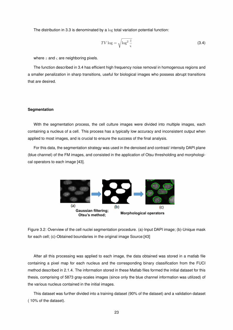
Segmentation

With the segmentation process, the cell culture images were divided into multiple images, each

containing a nucleus of a cell. This process has a typically low accuracy and inconsistent output when

applied to most images, and is crucial to ensure the success of the final analysis.

For this data, the segmentation strategy was used in the denoised and contrast/ intensity DAPI plane

(blue channel) of the FM images, and consisted in the application of Otsu thresholding and morphologi-

cal operators to each image [43].

Figure 3.2: Overview of the cell nuclei segmentation procedure. (a)-Input DAPI image; (b)-Unique mask

for each cell; (c)-Obtained boundaries in the original image Source:[43]

After all this processing was applied to each image, the data obtained was stored in a matlab file

containing a pixel map for each nucleus and the corresponding binary classification from the FUCI

method described in 2.1.4. The information stored in these Matlab files formed the initial dataset for this

thesis, comprising of 5873 gray-scales images (since only the blue channel information was utilized) of

the various nucleus contained in the initial images.

This dataset was further divided into a training dataset (90% of the dataset) and a validation dataset

( 10% of the dataset).

23

3.2 Methods

3.2.1 Machine Learning

To determine the cellular stage of each cell and have the ability to classify each nucleus indepen-

dently (i.e. not rely in clustering methods), machine learning algorithms were employed. Namely artificial

neural networks (ANN) and convolutional neural networks (CNN).

Neural Networks

Feature extraction The first step in using an ANN to learn the cellular stage, was to select and extract

relevant features from the dataset. As described in 2.1.2, one of the key defining characteristics of the

progression along the cell cycle is the variation of genetic material. In particular, the duplication of DNA

is a key characteristic of the S phase as is the growth of the nucleus in the G1 and G2 phases.

As such, the variation of genetic material contained in the cell and the variation of the nucleus size

were selected as the defining characteristics to express the cellular stage. To translate this behavior into

features capable of being used in training an ANN, the area and intensity of the nucleus were selected.

Each feature was expressed mathematically. The area was defined as the total number of pixels

contained in a nucleus (NP) limited by boundaries i′ and j′ such as:

Area =∑

i<i′,j<j′

NPi,j (3.5)

The total intensity was defined as the sum of the intensity of each pixel in the nucleus (as shown

below) and, theoretically, reflects the amount of DNA contained in each cell.

Area =

∫A

intensitydA =

T∑i=1

Intensityi (3.6)

By plotting each nucleus’ intensity and area, as shown in figure 3.3, one should expect to identify

three different concentrations of points:

• a first group of cells in G1 phase, with a significant rise in area and intensity, characteristic of cell

growth

• a second group of cells in S phase, with constant area and intensity increase which represents the

DNA duplication that occurs during this phase

• a third and final group of cells in G2 phase, with almost double area and intensity than in G1 which

represents the cell’s final growth corresponding to this phase

Data normalization After extracting the features, data normalization was applied to the data set,

namely, z-score normalization.

Data normalization is a common pre-processing technique to minimize the impact features with dif-

ferent ranges have in the final outcome. Potentially, features with larger ranges would have a higher

24

Figure 3.3: Scatter plot representing area and intensity of biological data

contribution for the final outcome than the features expressed in a smaller range. Furthermore attributes

should be dimensionless so that the unit of measure does not impact the final output. As previously

stated the method used was the z-score normalization, which can be defined as [46]:

x∗ij =xij − τij

σj(3.7)

where x∗ij is the normalized attribute value, xij represents the raw data and τj and σ represent the

mean and standard deviation (STD) for the values of the jth attribute. Z-score normalization returns a

dataset with 0 average and standard deviation of 1 and is one of the most commonly employed stan-

dardization techniques. [47, 48]

Designing and training the ANN With the features extracted and the visual classification from the

FUCCI method, a supervised learning method was employed to train an ANN.

To size the required network it was first created a network that could ”memorize” the problem, i.e.

overfit the dataset, and then overfitting prevention methods were applied. For this, the drop-out technique

was employed.

In this method the term dropout refers to ”dropping” units in a neural network along with incoming

and outgoing connections, as shown in figure 3.4. The choice of which nodes to drop is random, with a

fixed independent probability of p for each unit to drop. p can be selected from a test dataset, however

a probability of 50%, i.e. p = 0.5 seems to be optimal for most neural network problems [49].

By dropping units, essentially a thinned network is trained each time and is formed by all the remain-

ing units. As such, training a network with elements can be seen as training a set of 2n thinned networks

with weight sharing.

This approach poses the problem that at test time it is not feasible to express the average output of

25

so many thinned layers. However, a good approximation is to use a neural network without the dropout

where the weights of each hidden unit is multiplied by p at validation time [49]. This simple averaging

method ensures that the expected output of each hidden unit at test time is the same as during the

training phase. Thus, effectively combining 2n networks into a larger single neural network that can be

used at test time.

Figure 3.4: Dropout Neural Net Model. Left: A standard neural network with 2 hidden layers. Right: An

example of a thinned net produced by applying dropout to the net network on the left. Source:[49]

To adjust the training of the designed network 3 parameters were adjusted [27]:

• Epochs - Parameter that defines the number of times the learning algorithm will work the entire

data set

• Batch size - Parameter that defines the number of samples that are processed before the model

is updated

• Learning rate Parameter that defines how much the weights in a neural network are updated on

each batch

• Learning rate Parameter that defines how much the weights in a neural network are updated on

each batch

• Loss function Parameter that defines how the error or loss is determined with each batch

These parameters are correlated among them, for example, smaller learning rates require more

training epochs since each update has a smaller effect on the weights. On the other hand, batch size

determines the number of times the error function is determined per epoch and subsequently the number

of times the model weights are updated in each epoch.

There is no exact way to determine the value for each one of the parameters, with an empirical

process being required to determine the best solution for each problem. In the context of this thesis, after

various tests a large number of epochs were used in conjunction with overfitting prevention methods and

the mini-batch gradient descent method was used [50] (when batch size is smaller than the sample size,

resulting in multiple batches per epoch) with a small learning rate to ensure convergence.

26

For the loss function, binary cross entropy loss function was used and it can be defined as:

CE =

−log(f(s1)) if t1 = 1

−log(1− f(s1)) if t1 = 0(3.8)

where s1 and t1 are the score and the ground truth label for the class C1, and where t1 = 1 means

that class C1 = Ci is positive for this example. [51]

In addition to minimizing the loss function, the overall accuracy of the model was also monitored

during training, which can be defined as:

Accuracy =TP + TN

TP + TN + FP + FN(3.9)

where TP is true positives, FP is false positives, TN is true negatives and FN is false negatives.

In the end, an ANN with 10 layers of 1000 elements each was trained and optimized using the Adam

optimizer.

Convolutional Neural Networks

Image generation Contrary to ANN’s, and as explained in chapter 2, CNNs are capable of feature

detection and selection. As such, instead of extracting the features, as done for the ANN method,

150×150 pixel images were produced from the information contained in the Matlab files generated by

the preprocessing pipeline previously explained in this chapter and used as input. Figure 3.5 represents

one of the images generated for every nucleus contained in the information.

Figure 3.5: Image generated from processed pipeline and used as input for the CNN.

Data augmentation The use of CNNs for image classification requires a large amount of data to pre-

vent overfitting. Unfortunately, the original data set only presented 5873 nucleus and, as such, data

27

augmentation, a data-space solution to the problem of limited information for deep learning, was em-

ployed during this work.[52].

While not the only solution to overfitting in deep neural networks, data augmentation addresses the

problem at its root, the training data set, by assuming more information can be extracted from the original

data through augmentation. To extract this additional information, data augmentation methods typically

inflate the training dataset size by either data warping or oversampling, with techniques from geometric

and color transformations to random erasing, adversarial training or neural style transfer. [52]

During this project, and since the two classes considered were balanced in the available data-set ,

only data warping was employed. However, the main goal of data augmentation is to inflate the available

data while keeping the label of each data point valid. Below are some descriptions of geometrical

transformation techniques [52]:

• Flipping - Flipping corresponds to the transformation where an image is flipped across either on

the horizontal axis, the vertical axis or both;

• Color space - Color space augmentation describes techniques where color channels are manipu-

lated. One simple example of these techniques is isolating only of the RGB channels or changing

the intensity values of a image describing color histogram;

• Cropping - Cropping corresponds to extracting a patch from the total image. It is particularly useful

in processing images with mixed height and width dimensions;

• Rotation - Rotation corresponds to rotating the image either left or right on an axis between 1◦ and

359◦ ;

• Translation - Translations are performed by moving the image up, down, right or left, and are

particularly useful in removing positional bias from the images;

• Noise injection - Noise injection consists of injecting a matrix of random values usually drawn

from a Gaussian distribution.

Since the two most relevant features for describing the progression in the cell cycle are area and

intensity a careful selection of the techniques employed is required to ensure these features are not

perturbed and negatively affect the outcome. As such, from the methods described, only rotation, flipping

and translations did not affect the area and intensity of the images used.

Designing and training the CNN While data augmentation prevents overfitting and helps the network

”learn” more robust features, it is not the only overfitting prevention method available. In addition to the

dropout method previously described, early stopping was used to ensure the designed network would

be perform optimally. This method consists of monitoring the validation accuracy and loss to detect

overfitting and training is then stopped before convergence [53].

These methods were then used to develop a simple CNN network with only 2 fully connected con-

volutional layers and 1 hidden layer of 256 nodes, which was trained utilizing a large number of epochs

28

with the mini-batch gradient descent method, binary cross entropy loss function and Adam optimizer,

similarly to the training process used with the ANN.

3.3 Validation

3.3.1 MNIST dataset

While the MNIST dataset presents a different problem (multiclass vs binary classification, gray-scale

vs binary input) and input structure, this dataset was utilized to understand and validate the design

methodologies used. As such, both an ANN and CNN networks similar to the ones used were tested

against the modified National Institute of Standards and Technology (MNIST) data set [54]. This dataset

contains images from handwritten digits and is one of the most common starting points for neural net-

works with the performance of various types of networks well documented.

The MNIST was derived from the original NIST and contains a total of 60,000 training images and

10,000 test images, obtained from the same distribution. The data was normalized into black and white

digits, and centered in a fixed size image where the center of gravity of the intensity lies at the center of

the image[54], which is translated into a 28 × 28 grid where each value is binary. This relatively simple

database is ideal to test and validate methods since students and educators of machine learning can

benefit from a rather comprehensive set of machine learning literature with performance comparison

readily available.

Figure 3.6: MNIST database image sample. Source:[55]

By testing both the ANN and CNN networks with this data set, a validation error of<8% was achieved

for both of them. While below the results already achieved by other networks, the goal was simply to

validate the training and design methods and no fine-tunning was performed to increase the accuracy

on this dataset.

29

3.3.2 VGG Network

In addition to using the MNIST data set for validation, a pre-trained VGG network was used as a

benchmark for the convolutional neural network.

The VGG network has an architecture with very small (3x3) convolution filters followed by sixteen

to nineteen weight layers and was proposed for the ImageNet challenge [56]. This challenge uses a

sample of the ImageNet dataset of approximately 1000 categories with 1000 images per category. The

VGG was submitted for 2014 challenge by K. Simonyan and A. Zisserman from the University of Oxford

and achieved 92.7% top-5 test accuracy in that competition. This represented an improvement over

prior-art (namely the AlexNet [57] network) and has become one of the benchmark networks for this

challenge.

While the ImageNet challenge has a larger dataset and is not exactly comparable to the data avail-

able for this project due to the difference in input format and number of channels used, the availability

of various configurations of pre-trained VGG16 networks and the widely available bibiography on this

network led to its choice as a benchmark.

Figure 3.7: VGG16 architecture. Source:[58]

30

Chapter 4

Results

In this section, the results obtained during this work are presented. First, the results for the artificial

neural network are shown with a demonstration of the overfitting prevention methods followed by the

demonstration of the results obtained utilizing the convolutional neural network.

4.1 Artificial Neural Network

On this section, the results obtained during the use of artificial neural networks will be demonstrated,

both the efficiency of the overfitting prevention methods and the overall result from the trained network.

After extracting the selected features from the biological dataset, area and intensity, these were

subjected to classification using an artificial network. As illustrated in figure 4.1, the designed network

was capable of overfitting the problem. This is evidenced by the separation between the validation loss

and the training loss represented in figure 4.1(a).

Figure 4.1(b) represents the accuracy evolution of the same training, and while the initial weights

loaded into the network provided a good starting point, without overfitting prevention methods, the val-

idation accuracy was unstable and it did not increase, showing the models inability to generalize the

information acquired during training.

Figure 4.2 shows the training evolution of the same network with overfitting prevention methods

used, namely the use of dropout. As is evidenced by 4.2(a), in this case, while not exactly converging,

the training loss and the validation loss do not diverge as the network is trained, which evidences the

effectiveness of the dropout method to prevent overfiting. In figure 4.2(b), the evolution of the accuracy

in each epoch is evidenced, showing a stabilization of the validation around 70%.

To simulate early stopping, the best performing network was saved and then tested against a val-

idation set that was not used during training and evaluated across 2 metrics in addition to accuracy:

sensitivity and specificity which can be defined as follows:

Sensitivity =TP

TP + FNSpecificity =

TN

TN + FP

31

(a) Loss evolution per epoch (b) Accuracy evolution per epoch

Figure 4.1: Training and validation metrics for ANN without dropout method. Left: Validation and trainingloss per epoch; Right: Validation and training accuracy per epoch.

(a) Loss evolution per epoch (b) Accuracy evolution per epoch

Figure 4.2: Training and validation metrics for ANN with dropout method. Left: Validation and trainingloss per epoch; Right: Validation and training accuracy per epoch.

where TP is true positives, FP is false positives, TN is true negatives and FN is false negatives.

Overall the obtained results for the final ANN were:

Senstivity Specificity Accuracy

73,13% 78,81% 76,21%

Table 4.1: ANN validation results.

While above the convergence accuracy, the validation set corresponds to only 10% of the original

data set of ≈ 6000 points, which corresponds to a small amount. However, accuracy for this method

remains above 70% in any test set of the original data which are promising results.

4.2 Convolutional Neural Network

On this section, the results obtained from the use of convolutional neural networks will be demon-

strated.

32

Figure 4.3 represents the evolution of the CNN metrics during training. As shown in figure 4.3(a), the

loss started reducing, however from approximately epoch 75 onwards it is clear the training is resulting in

some overfitting. This is also evidenced in figure 4.3(b) where the validation accuracy starts decreasing

while training accuracy evolves.

(a) Loss evolution per epoch (b) Accuracy evolution per epoch

Figure 4.3: Training and validation metrics for CNN trained with synthetic data. Left: Validation and

training loss per epoch; Right: Validation and training accuracy per epoch.

To simulate early stopping, the best performing network weights were saved and used to further fine

tune the network training parameters in order to increase the accuracy. In particular, the learning rate

was reduced to facilitate the convergence of the validation metrics with the training metrics. Below are

the results achieved with this fine tuning:

(a) Loss evolution per epoch (b) Accuracy evolution per epoch

Figure 4.4: Training and validation metrics for CNN fin tuned with synthetic data. Left: Validation and

training loss per epoch; Right: Validation and training accuracy per epoch.

As evidenced in figure 4.4, reducing the learning rate helped improve the CNN accuracy and reduce

its loss while avoiding overfitting.

Once again, the weights of the best performing CNN were used to assess the network performance

across the same metrics as the ANN. Below are the results:

33

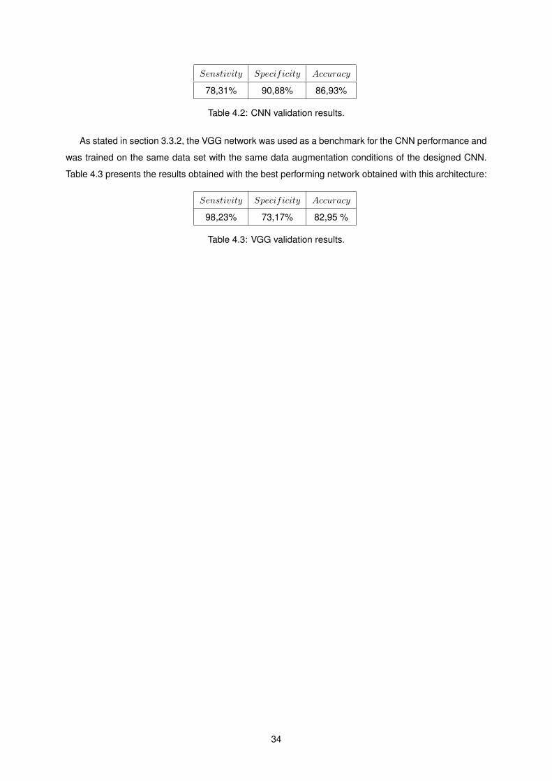
Senstivity Specificity Accuracy

78,31% 90,88% 86,93%

Table 4.2: CNN validation results.

As stated in section 3.3.2, the VGG network was used as a benchmark for the CNN performance and

was trained on the same data set with the same data augmentation conditions of the designed CNN.

Table 4.3 presents the results obtained with the best performing network obtained with this architecture:

Senstivity Specificity Accuracy

98,23% 73,17% 82,95 %

Table 4.3: VGG validation results.

34

Chapter 5

Conclusions

The following section will present the achievements of this thesis and delineate a path for future work.

5.1 Achievements

Based on FM images obtained of in vivo cell cultures, the primary goal of this thesis was to develop

a simple way of correctly identifying the cell phase of a particular cell.

Currently, FM based methods for accessing the cell status of individual cells are only capable of

probing specific parts of the cell cycle, such as metabolic labeling procedures who only identify cells

transversing the S-Phase [59] or staining methods who rely on specific cell markers [60], or are very

laborious since they evolve the growth of cultures with phase specific identifiers, such as the FUCCI

method used as validation for this work. While some of these second methods are capable of monitoring

all phases in the cell cycle, they are not universal and are dependent on the cellular system chosen. This

approach results in a very complex process which requires the use of multiple imaging channels and

inhibit the capability to visualize other cell features in the same culture.

By contrast, the method suggested in this thesis relies on the use of a inexpensive and commonly

used compound, the DNA dying die DAPI. This compound, allows the extraction of information from

fluorescence imaging thanks to the image processing pipeline explained in section 3. Particularly, it

allows the extraction of information representing both the nucleus area and the amount of DNA, two

intrinsic features who provide a good description of the cell status along its cellular cycle.

While some other machine learning methods rely on the information gathered from the DAPI stain

have already been proposed [43] with good results (accuracy > 95%), they relied on the use of clustering

algorithms which require the use of information gathered from an entire cell culture and are not capable

of identifying a single data point. The method proposed for this thesis implemented the use of deep

learning techniques, that were capable, after proper training, of identifying the cell phase from a single

data point, not requiring information from entire cell cultures after the training phase was completed. To

achieve this goal, both an ANN and a CNN were used to analyze and classify the data set obtained from

the FUCCI stained cell cultures.

35

The ANN method relied on the manual extraction of the intrinsic features of the nucleus, area and

intensity, that should translate adequately the cell phase of a single nucleus. By using this method

an accuracy of ≈ 76% was obtained when classifying cells in either the G1 or the S/G2/M phase. A

result which, while lower than the accuracy obtained in clustering methods, it still demonstrates a clear

correlation between the selected features and the cell phase. One possible explanation for this difference

in accuracy is potentially the data normalization technique used. Combining the fluorescence images

from various cultures, which were obtained at different times from cultures that could have reacted

differently to the staining procedure, was essential to uniformize the data set. However, as a result of

this normalization it is possible that some data points might have lost their correlation between their

features and their label.

In addition to the ANN method, two CNNs were also used in this thesis in conjunction with data

augmentation techniques. The first network was a self designed simple CNN with only two convulational

layers which produced an accuracy of ≈ 87% while the second network used was resorted to the archi-

tecture of a VGG network which produced an accuracy of ≈ 83%. Both of these networks did not rely on

the manual extraction of features, rather relying on the automatic identification of features that translated

the cell phase. While the results achieved are still below the ones obtained with clustering algorithms,

the increase in accuracy compared with the ANN still demonstrates that the use of a CNN to address

image based cell classification is a promising solution. Particularly, the further fine tune of the VGG net-

work used could result in accuracy results comparable to the one’s achieved with clustering methods,

since limited fine tuning was performed in this network due to its heavy computational requirements to

train which limited its development during this work.

While below the results accomplished with clustering methods, the results achieved with the methods

proposed were very satisfactory and represent a promising solution to the problem of image based cell

classification for a single nucleus.

5.2 Future Work

As previously stated, the use of deep learning techniques resulted in promising results to analyze

and classify the cell phase through the use of fluorescence images. Particularly, the use of CNNs has

shown potential as a solution for this problem.

As such, a more complex CNN should be used and fine-tuned with a larger dataset than the one

currently available to try and improve the results obtained during this work.

Additionally, a multi class classification should be tried instead of the current binary one to distinguish

between the different phases in the current class of the G2/S/M. However, to implement this classifier

in a supervised learning method as the ones used here, other biological imaging techniques would be

required to produce the validation information for the data set.

36

Bibliography

[1] M. Malumbres and M. Barbacid. Cell cycle, cdks and cancer: a changing paradigm. Nature Reviews

Cancer, 9:153–166, 2009.

[2] D. Hanahan and R. A. Weinberg. Hallmarks of cancer: The next generation. Cell, 144(5):646 –

674, 2011.

[3] D. Jackson and P. R. Cook. Analyzing dna replication i: Labeling animals, tissues, and cells with

bromodeoxyuridine (brdu). Cold Spring Harbor Protocols, 2008(8):pdb.prot5031, 2008.

[4] M. Hesse, A. Raulf, G.-A. Pilz, C. Haberlandt, A. M. Klein, R. Jabs, H. Zaehres, C. J. Fugemann,

K. Zimmermann, J. Trebicka, A. Welz, A. Pfeifer, W. Roll, M. I. Kotlikoff, C. Steinhauser, M. Gotz,

H. R. Scholer, and B. K. Fleischmann. Direct visualization of cell division using high-resolution

imaging of m-phase of the cell cycle. Nature Communications, 3:1076, 2012.

[5] G. V.-T. C. M. T. Roukos, Vassilisand Pegoraro. Cell cycle staging of individual cells by fluorescence

microscopy. 10:334–348, 2015.

[6] Y. Nagao, M. Sakamoto, T. Chinen, Y. Okada, and D. Takao. Robust classification of cell cycle

phase and biological feature extraction by image-based deep learning. Molecular Biology of the

Cell, pages mbc–E20, 2020.

[7] C. L. Chen, A. Mahjoubfar, L.-C. Tai, I. K. Blaby, A. Huang, K. R. Niazi, and B. Jalali. Deep learning

in label-free cell classification. Scientific reports, 6:21471, 2016.

[8] C. M. O’Connor and J. U. Adams. Essentials of Cell Biology. NPG Education, 2010.

[9] B. Editors. Eukaryotic cell. https://biologydictionary.net/eukaryotic-cell/.

[10] C. M. O’Connor and J. U. Adams. Essentials of Cell Biology. NPG Education, 2010.

[11] Chapter 40 - introduction to the cell cycle. In T. D. Pollard, W. C. Earnshaw, J. Lippincott-Schwartz,

and G. T. Johnson, editors, Cell Biology (Third Edition), pages 697 – 711. Elsevier, third edition edi-

tion, 2017. ISBN 978-0-323-34126-4. doi: https://doi.org/10.1016/B978-0-323-34126-4.00040-2.

URL http://www.sciencedirect.com/science/article/pii/B9780323341264000402.

[12] A. Carnero. Targeting the cell cycle for cancer therapy. British Journal of Cancer, 87:129–133,

2002.

37

[13] H. Kreipe and R. Parwaresch. A closer look at the cell cycle. Virchoes Archives, 422:341–343,

1993.

[14] M. C. Genome. Cell cycle control. https://www.mycancergenome.org/content/pathways/cell-cycle-

control/.

[15] M. Tessema, U. Lehmann, and H. Kreipe. Cell cycle and no end. Virchows Archive, 444(4):313–

323, 2004.

[16] J. Blow. Replication Licensing System, pages 3258–3262. Springer Berlin Heidelberg, Berlin,

Heidelberg, 2011. ISBN 978-3-642-16483-5. doi: 10.1007/978-3-642-16483-5 5037. URL https:

//doi.org/10.1007/978-3-642-16483-5_5037.

[17] M. Schwab. Encyclopedia of Cancer. Springer, 2009.

[18] C. M. O’Connor and J. U. Adams. Essentials of Cell Biology. NPG Education, 2010.

[19] U. of Leicester. The cell cycle, mitosis and meiosis. https://www2.le.ac.uk/projects/vgec/highereducation/topics/cellcycle-

mitosis-meiosis.

[20] X. Grana and E. P. Reddy. Cell cycle control in mammalian cells: role of cyclins, cyclin dependent

kinases (cdks) growth supressor genes and cyclin-dependent kinase inhibitors (ckis). Oncogene,

11:211–219, 1995.

[21] Z. T. irak. Investigation of tadf properties of novel donor-acceptor type pyrazine derivatives. Journal

of the Chilean Chemical Society, 64:4303 – 4309, 03 2019. ISSN 0717-9707.

[22] J. W. Lichtman and J.-A. Conchello. Fluorescence microscopy. Nature Methods, 2(12):910–919,

2005.

[23] B. I. Tarnowski, F. G. Spinale, and J. H. Nicholson. Dapi as a useful stain for nuclear quantitation.

Biotechnic & Histochemistry, 66(6):296–302, 1991.

[24] S. Hamada and S. Fujita. Dapi staining improved for quantitative cytofluorometry. Histochemistry,

79(2):219–226, 1983.

[25] A. Sakaue-Sawano, H. Kurokawa, T. Morimura, A. Hanyu, H. Hama, H. Osawa, S. Kashiwagi,

K. Fukami, T. Miyata, H. Miyoshi, T. Imamura, M. Ogawa, H. Masai, and A. Miyawaki. Visualizing

spatiotemporal dynamics of multicellular cell-cycle progression. Cell, 132(3):487 – 498, 2008.

[26] Fluorescent cellular changes associated with fucci cell cycle sensor, .

https://www.moleculardevices.com/en/assets/app-note/dd/img/evaluating-cell-cycle-inhibitors-

using-live-cell-assaygref.

[27] C. M. Bishop. Pattern Recognition and Machine Learning (Information Science and Statistics),

chapter 1, pages 1–12. Springer-Verlag, 2006.

38

[28] S. Russell and P. Norvig. Artificial Intelligence: A Modern Approach, chapter 18, pages 693–757.

Series in Artificial Intelligence. Prentice Hall, 3 edition, 2010.

[29] Y. LeCun. The power and limits of deep learning: In his iri medal address, yann lecun maps the

development of machine learning techniques and suggests what the future may hold. Research-

Technology Management, 61(6):22–27, 2018.

[30] Y. LeCun, Y. Bengio, and G. Hinton. Deep learning. Nature, 521:436–444, 2015.

[31] C. M. Bishop. Pattern Recognition and Machine Learning (Information Science and Statistics),

chapter 5, pages 225–284. Springer-Verlag, 2006.

[32] A review of the math used in training a neural network, . https://morioh.com/p/d70aa769173a.

[33] I. Goodfellow, Y. Bengio, and A. Courville. Deep Learning, chapter 6, pages 168–227. The MIT

Press, 2016.

[34] F. Bre, J. Gimenez, and V. Fachinotti. Prediction of wind pressure coefficients on building surfaces

using artificial neural networks. Energy and Buildings, 158, 11 2017.

[35] S. B. Kotsiantis, I. Zaharakis, and P. Pintelas. Supervised machine learning: A review of classifi-

cation techniques. Emerging artificial intelligence applications in computer engineering, 160:3–24,

2007.

[36] A. Abraham. Handbook of Measuring System Design, chapter Artificial Neural Networks. John

Wiley & Sons, Ltd., 2005.

[37] M. Gardner and S. Dorling. Artificial neural networks (the multilayer perceptron)—a review of appli-

cations in the atmospheric sciences. Atmospheric Environment, 32(14):2627 – 2636, 1998.

[38] I. Goodfellow, Y. Bengio, and A. Courville. Deep Learning, chapter 9, pages 330–372. The MIT

Press, 2016.

[39] C. M. Bishop. Pattern Recognition and Machine Learning (Information Science and Statistics),

chapter 5.5.6, pages 267–269. Springer-Verlag, 2006.

[40] Convolution-definition. http://mathworld.wolfram.com/Convolution.html. Accessed: 20-11-

2018.

[41] A. Krizhevsky, I. Sutskever, and G. E. Hinton. Imagenet classification with deep convolutional

neural networks. In F. Pereira, C. J. C. Burges, L. Bottou, and K. Q. Weinberger, editors, Advances

in Neural Information Processing Systems 25, pages 1097–1105. Curran Associates, Inc., 2012.

[42] A. Sakaue-Sawano, H. Kurokawa, T. Morimura, A. Hanyu, H. Hama, H. Osawa, S. Kashiwagi,

K. Fukami, T. Miyata, H. Miyoshi, T. Imamura, M. Ogawa, H. Masai, and A. Miyawaki. Visualizing

spatiotemporal dynamics of multicellular cell-cycle progression. Cell, 132(3):487 – 498, 2008. ISSN

0092-8674. doi: https://doi.org/10.1016/j.cell.2007.12.033. URL http://www.sciencedirect.com/

science/article/pii/S0092867408000548.

39

[43] I. Sahumbaiev. Cell cycle staging from dapi and fluorescence microscopy. Master’s thesis, Instituto

Superior Tecnico, 2015.

[44] M. Bertero and P. Boccacci. Introduction to inverse problems in imaging. CRC press, 1998.

[45] I. C. Rodrigues and J. M. R. Sanches. Convex total variation denoising of poisson fluorescence

confocal images with anisotropic filtering. IEEE Transactions on Image Processing, 20(1):146–160,

2011.

[46] M. Y. P. Maria M. Suarez-Alvarez, Duc-Truong Pham and Y. I. Prostov. Statistical approach to

normalization of feature vectors and clustering of mixed datasets. The Royal Society, 2012.

[47] G. Gan, C. Ma, and J. Wu. Data clustering: theory, algorithms, and applications. SIAM, 2007.

[48] G. W. Milligan and M. C. Cooper. A study of standardization of variables in cluster analysis. Journal

of classification, 5(2):181–204, 1988.

[49] N. Srivastava, G. Hinton, A. Krizhevsky, I. Sutskever, and R. Salakhutdinov. Dropout: a simple

way to prevent neural networks from overfitting. The journal of machine learning research, 15(1):

1929–1958, 2014.

[50] S. Khirirat, H. R. Feyzmahdavian, and M. Johansson. Mini-batch gradient descent: Faster conver-

gence under data sparsity. In 2017 IEEE 56th Annual Conference on Decision and Control (CDC),

pages 2880–2887, 2017.

[51] I. Goodfellow, Y. Bengio, and A. Courville. Deep Learning, chapter 1, pages 1–28. The MIT Press,

2016.

[52] C. Shorten and T. M. Khoshgoftaar. A survey on image data augmentation for deep learning.

Journal of Big Data, 6(1):60, Jul 2019.

[53] L. Prechelt. Early stopping-but when? In Neural Networks: Tricks of the trade, pages 55–69.

Springer, 1998.

[54] L. Deng. The mnist database of handwritten digit images for machine learning research [best of

the web]. IEEE Signal Processing Magazine, 29(6):141–142, 2012.

[55] Mnist reborn, restored and expanded: Additional 50k training samples, .

https://medium.com/syncedreview/mnist-reborn-restored-and-expanded-additional-50k-training-

samples-70c6f8a9e9a9.

[56] K. Simonyan and A. Zisserman. Very deep convolutional networks for large-scale image recogni-

tion. arXiv preprint arXiv:1409.1556, 2014.

[57] A. Krizhevsky, I. Sutskever, and G. E. Hinton. Imagenet classification with deep convolutional neural

networks. In Advances in neural information processing systems, pages 1097–1105, 2012.

40

[58] Vgg16 – convolutional network for classification and detection, . https://neurohive.io/en/popular-

networks/vgg16/.

[59] D. Jackson and P. R. Cook. Analyzing dna replication i: labeling animals, tissues, and cells with

bromodeoxyuridine (brdu). Cold Spring Harbor Protocols, 2008(8):pdb–prot5031, 2008.

[60] H. Leonhardt, H.-P. Rahn, P. Weinzierl, A. Sporbert, T. Cremer, D. Zink, and M. C. Cardoso. Dy-

namics of dna replication factories in living cells. The Journal of cell biology, 149(2):271–280,

2000.

41

42