Deep Learning of Invariant Spatio-Temporal Featuresfrom Video

by

Bo Chen

B Sc. Computing Science, Simon Fraser University, 2008

A THESIS SUBMITTED IN PARTIAL FULFILLMENT

OF THE REQUIREMENTS FOR THE DEGREE OF

Master of Science

in

THE FACULTY OF GRADUATE STUDIES

(Computer Science)

The University of British Columbia

(Vancouver)

August 2010

c© Bo Chen, 2010

Abstract

We present a novel hierarchical and distributed model for learning invariant spatio-

temporal features from video. Our approach builds on previous deep learning

methods and uses the Convolutional Restricted Boltzmann machine (CRBM) as

a building block. Our model, called the Space-Time Deep Belief Network (ST-

DBN), aggregates over both space and time in an alternating way so that higher

layers capture more distant events in space and time. The model is learned in

an unsupervised manner. The experiments show that it has good invariance proper-

ties, that it is well-suited for recognition tasks, and that it has reasonable generative

properties that enable it to denoise video and produce spatio-temporal predictions.

ii

Table of Contents

Abstract . . . . . . . . . . . . . . . . . . . . . . . . . . . . . . . . . . . ii

Table of Contents . . . . . . . . . . . . . . . . . . . . . . . . . . . . . . iii

List of Tables . . . . . . . . . . . . . . . . . . . . . . . . . . . . . . . . . v

List of Figures . . . . . . . . . . . . . . . . . . . . . . . . . . . . . . . . vi

Acknowledgments . . . . . . . . . . . . . . . . . . . . . . . . . . . . . . viii

1 Introduction . . . . . . . . . . . . . . . . . . . . . . . . . . . . . . . 11.1 Thesis Contribution . . . . . . . . . . . . . . . . . . . . . . . . . 2

1.2 Thesis Organization . . . . . . . . . . . . . . . . . . . . . . . . . 2

2 Principles and Models of the Human Visual System . . . . . . . . . 32.1 Principles of the Vision Cortex . . . . . . . . . . . . . . . . . . . 3

2.1.1 Hierarchical Representations . . . . . . . . . . . . . . . . 3

2.1.2 Invariance . . . . . . . . . . . . . . . . . . . . . . . . . . 4

2.1.3 Sparseness . . . . . . . . . . . . . . . . . . . . . . . . . 5

2.2 Models Inspired by the Visual Cortex . . . . . . . . . . . . . . . 5

2.2.1 The Simple-Complex Cell Model . . . . . . . . . . . . . 6

2.2.2 Sparse Coding . . . . . . . . . . . . . . . . . . . . . . . 7

2.2.3 Feedforward Neural Networks . . . . . . . . . . . . . . . 7

2.2.4 Undirected Neural Networks . . . . . . . . . . . . . . . . 8

2.3 Summary . . . . . . . . . . . . . . . . . . . . . . . . . . . . . . 10

3 Feature Extraction from Video . . . . . . . . . . . . . . . . . . . . . 11

iii

4 Convolutional Restricted Boltzmann Machines . . . . . . . . . . . . 134.1 Restricted Boltzmann Machines . . . . . . . . . . . . . . . . . . 13

4.1.1 Model . . . . . . . . . . . . . . . . . . . . . . . . . . . . 13

4.1.2 Inference and Learning . . . . . . . . . . . . . . . . . . . 15

4.1.3 RBMs in Computer Vision . . . . . . . . . . . . . . . . . 17

4.2 Convolutional Restricted Boltzmann Machines (CRBMs) . . . . . 17

4.2.1 Cross-Correlation and Convolution . . . . . . . . . . . . 18

4.2.2 Model . . . . . . . . . . . . . . . . . . . . . . . . . . . . 19

4.2.3 Training . . . . . . . . . . . . . . . . . . . . . . . . . . . 22

4.2.4 Limitations of the CRBM . . . . . . . . . . . . . . . . . 24

5 The Space-Time Deep Belief Network . . . . . . . . . . . . . . . . . 255.1 Model . . . . . . . . . . . . . . . . . . . . . . . . . . . . . . . . 25

5.2 Training and Inference . . . . . . . . . . . . . . . . . . . . . . . 27

6 ST-DBN as a Discriminative Feature Extractor . . . . . . . . . . . . 316.1 Measuring Invariance . . . . . . . . . . . . . . . . . . . . . . . . 31

6.1.1 Dataset and Training . . . . . . . . . . . . . . . . . . . . 31

6.1.2 Invariance Measure . . . . . . . . . . . . . . . . . . . . . 32

6.2 Unsupervised Feature Learning for Classification . . . . . . . . . 34

6.2.1 Dataset and Training . . . . . . . . . . . . . . . . . . . . 34

6.2.2 Classification Performance . . . . . . . . . . . . . . . . . 36

6.2.3 Discussion . . . . . . . . . . . . . . . . . . . . . . . . . 37

7 ST-DBN as a Generative Model . . . . . . . . . . . . . . . . . . . . 387.1 Denoising . . . . . . . . . . . . . . . . . . . . . . . . . . . . . . 38

7.2 Prediction . . . . . . . . . . . . . . . . . . . . . . . . . . . . . . 39

8 Discussion and Conclusions . . . . . . . . . . . . . . . . . . . . . . 418.1 Discussion . . . . . . . . . . . . . . . . . . . . . . . . . . . . . . 41

8.2 Conclusions . . . . . . . . . . . . . . . . . . . . . . . . . . . . . 42

Bibliography . . . . . . . . . . . . . . . . . . . . . . . . . . . . . . . . . 43

iv

List of Tables

Table 2.1 A comparison of selected computational models that mimic the

human visual system. Each column is a desirable property. The

“Invariant” column shows the type of transformations to which

the system is invariant. “G”,“T” , “S” and “R” denote generic

transformations, translation, scale and rotation, respectively. . 10

Table 6.1 Average classification accuracy results for KTH actions dataset. 36

v

List of Figures

Figure 4.1 Computational flow of feature extraction using a CRBM for

one input frame. Directed edges shows the feedforward com-

putational flow. The underlying generative model has undi-

rected edges. . . . . . . . . . . . . . . . . . . . . . . . . . . 20

Figure 5.1 Illustration of the flow of computation in a ST-DBN feature

extractor. ST-DBN aggregates spatial information, shrinking

the resolution in space, and then aggregates over time, shrink-

ing the resolution in time, and repeats until the representation

becomes sufficiently small. . . . . . . . . . . . . . . . . . . . 26

Figure 5.2 Feature extraction in the spatial pooling layer for an input video

with nVt frames. Each input frame is fed into a CRBM. . . . 27

Figure 5.3 Feature extraction in the temporal pooling layer. Each pixel

sequence is fed into a CRBM. . . . . . . . . . . . . . . . . . 28

Figure 6.1 Invariance scores for common transformations in natural videos,

computed for layer 1 (S1) and layer 2 (S2) of a CDBN and

layer 2 (T1) of ST-DBN. (Higher is better.) . . . . . . . . . . 33

Figure 6.2 Learned layer one and layer two ST-DBN filters on KTH. For

the first layer (left), each square shows a 8×8 spatial filter. For

the second layer (right), each row shows a temporal filter over

6 time steps. . . . . . . . . . . . . . . . . . . . . . . . . . . 35

Figure 7.1 Denoising results: (a) Test frame; (b) Test frame corrupted

with noise; (c) Reconstruction using 1-layer ST-DBN; (d) Re-

construction with 2-layer ST-DBN. . . . . . . . . . . . . . . 39

vi

Figure 7.2 Top video shows an observed sequence of gazes/foci of atten-

tion (i.e., frames 2-4). Bottom video shows reconstructions

within the gaze windows and predictions outside them. . . . . 40

vii

Acknowledgments

I would like to express my gratitude to many people, who have made me a better

researcher and without whom this thesis would not have been written: most of all,

my supervisor Nando de Freitas, for his invaluable guidance, continuing support

and infinite optimism throughout the ups and downs of my degree. Jo-Anne Ting,

for her helpful feedbacks on my thesis and for being the best communicator and

collaborator I have ever met. Doctor Benjamin Marlin, professors Jim Little, David

Lowe, Greg Mori and Kevin Murphy for their rewarding discussions and brilliant

advice. The wonderful people at UBC and SFU: Eric Brochu, David Duvenaud,

Jiawei Huang, Emtiyaz Khan, Nimalan Mahendran, Kevin Swersky and Haiyang

Wang, just to name a few, for sharing their clever ideas or challenging problems

with me. And last but not least, my parents Hong Luo and Hongji Chen, for their

deep and invariant love that travels through the vast space across the Pacific Ocean

and lasts through the unforgettable time of my Master’s degree.

viii

Chapter 1

Introduction

Unsupervised feature learning is a challenging but crucial step towards building

robust visual representations. Such representations can be used for a myriad of

tasks from low-level ones like image denoising, inpainting and reconstruction to

higher-level ones like object and activity recognition. A general consensus on the

desirable properties of a feature extractor has emerged from the body of literature

on neuroscience and unsupervised feature learning, and these include the follow-

ing:

i. hierarchical distributed representation (for memory and generalization

efficiency [4, 29])

ii. feature invariance (for selectivity and robustness to input transformations [15,

23, 53])

iii. generative properties for inference (e.g., denoising, reconstruction, predic-

tion, analogy-learning [19, 29, 32])

iv. good discriminative performance (for object and action recognition [8, 33])

v. at the expense of re-iterating, unsupervised learning of features because of

the lack of supervisory signals in many sources of data.

In addition, learning from large-scale spatio-temporal data such as videos can

be computationally intensive and presents yet another challenge.

We propose a hierarchical, distributed probabilistic model for unsupervised

learning of invariant spatio-temporal features from video. Our work builds upon

1

recently proposed deep learning approaches [5, 19, 41]. In particular, we adopt the

convolutional Restricted Boltzmann machine (CRBM), previously introduced for

static images [9, 29, 35], as the basic building block in the architecture due to its

previously reported success [29].

Our architecture, called the Space-Time Deep Belief Network (ST-DBN), ag-

gregates over both time and space in an alternating fashion so that higher layers

capture more distant events in space and time. As a result, even if an image patch

changes rapidly from frame to frame, objects in the video vary slowly at higher

levels of the hierarchy.

1.1 Thesis ContributionOur model fulfills all the desirable properties listed above. We build feature in-

variance in a similar fashion to approaches such as Slow Feature Analysis [53] and

Hierarchical Temporal Memory [16]. However, the nodes of our hierarchy learn

and encode distributed feature representations (having higher complexity in higher

layers of the hierarchy). Our model is generative and, hence, able to deal with

occlusions in video and to make predictions that account for image content and

transformations. Moreover, it extracts features that lend themselves naturally to

discriminative tasks such as object and motion recognition.

1.2 Thesis OrganizationThis thesis is organized as follows: in chapter 2 we review computational principles

of the human visual system to provide biological motivation for our work. Then

we give an overview of feature extraction techniques from spatiotemporal data in

chapter 3. In chapter 4 we review CRBMs, and in chapter 5 we introduce the

proposed model, STDBN, which composes CRBMs into a multilayered model for

videos. The STDBN can be used both in a discriminative setting and in a generative

setting, which we investigate in chapter 6 and chapter 7, respectively. Finally we

discuss the limitations and extensions of STDBN and conclude in chapter 8.

2

Chapter 2

Principles and Models of theHuman Visual System

Despite continuous progress in the design of artificial visual systems, the human

visual system remains the most successful one in a myriad of challenging visual

tasks. This success can be largely attributed to the visual system’s neuronal rep-

resentation of the visual world. In this chapter, we provide a general overview

of three learning principles of the human visual system and discuss a few of the

computational models that partially implement these principles.

2.1 Principles of the Vision CortexHere we outline three of the most well-recognized principles of the visual cortex:

hierarchical representations, invariance and sparseness.

2.1.1 Hierarchical Representations

The first and the most important principle of the visual cortex is a hierarchical

structure for computation and information. The connectivity of the visual cortex

suggests that visual information is processed in a deep hierarchy: for example, the

ventral pathway, which is where object recognition is done, follows the path which

consists of areas such as the retina, lateral geniculate nucleus (LGN), visual area

3

1(V1), visual area 2 (V2), visual area 4 (V4), and inferotemporal area (IT) [52]1.

There is also an abstraction hierarchy. For example, in LGN, there is a point-to-

point connectivity that reflects the light intensity of every location in the retina.

As we proceed up the hierarchy, higher layers compose information from layers

below to form more abstract concepts, gradually losing the point-to-point connec-

tivity. Eventually at IT, neuron firings become insensitive to the location of input

signals. The final aspect of the hierarchical organization is that layers across the

hierarchy have a common learning module. As an example, the visual cortex com-

prises a large number of micro-columns that share a common, six-layered structure.

These micro-columns are grouped into visual areas by sets of dominating external

connections [34].

The hierarchical organization principle provides memory and generalization

efficiency [4]. It is memory efficient because the neuronal representation can de-

scribe complex objects in terms of its simpler components. Similarly, hierarchical

composition of previously learned features leads to novel feature generation, allow-

ing for efficient generalization without having to learn new features “from scratch”.

2.1.2 Invariance

The second principle of the human visual system is its ability to recognize an ob-

ject despite variations in the object’s presentation. Special types of neurons called

“complex cells” are found to fire for a visual stimulus largely independent of its

location [20]. Similarly, neuronal responses that are invariant to scale [21, 37] and

viewpoint [6] are discovered experimentally. More astonishingly, it has been re-

ported in a study [39] that there probably exist some neurons that fire for concepts

such as Halle Berry. That is, these neurons are triggered by photographs of Halle

as well as her name in text. Although it is inconclusive as to whether these cells fire

exclusively for the concept of “Halle Berry”, the study nonetheless demonstrates

the robustness of neuronal encoding.

Invariance is a highly desirable property, but it is debatable how it is learned in

the visual cortex. One conjecture is that temporal coherence [3, 13, 53] is the key

1This only gives a coarse approximation to the true neuronal connectivity and the actual infor-mation processing pathway. Some connections, such as the shortcut between V1 and V4, are notmodeled.

4

to learning invariant representations. Temporal coherence assumes that in natural

videos, successive frames are likely to contain the same set of concepts — hence,

the neuronal representation should change slowly in time. Since sequential data

is abundant, learning from temporal coherence in sequential data provides an rich

source of learning signal, and is believed to be more biologically plausible [17].

2.1.3 Sparseness

The third principle of the human visual system is sparsity. When natural images are

presented to primates, only a small portion of the neurons in V1 are activated [49].

This property is also true for the auditory system [10] and the olfactory system [38].

Sparse coding is advantageous because the resultant neuronal coding is inter-

pretable and energy efficient [2]. Interpretability means that neurons tend to fire

to represent the presence of common structures, i.e. features, in natural images.

Hence, it is easy to read off the content of an image by probing the population

of stimulated neurons. Sparsity also reduces the total energy consumption of the

visual cortex. Neuronal firing consumes energy, hence the brain can not afford

continuous stimulation of a large portion of its neurons [2].

2.2 Models Inspired by the Visual CortexThere is a significant number of models that implement one or a few of the above-

stated principles. Hence, an extensive review is impractical. Instead, we describe a

few relevant ones, with emphasis on unsupervised models in the machine learning

community.

Before reviewing the models, we describe common strategies to implement the

three principles of neuronal representations mentioned in Sec. 2.1. The hierarchical

organization principle is implemented by stacking some basic learning modules on

top of each other to form a multi-layered network. The invariance principle is im-

plemented by either hand-wiring the model structure to account for specific types

of transformations or learning temporally coherent representations from videos.

One of the most typical model structure is the combination of convolution and

resolution reduction. Convolution, which will be discussed in detail in Sec. 4.2,

assumes that local image statistics can be replicated globally in the image and is

5

advantageous for building efficient, scalable visual systems. Resolution reduction

ignores small shifts of the local image statistics and provides translational invari-

ance. Finally, the sparsity principle is implemented by imposing sparsity-inducing

priors or regularizers on the system’s representation of images.

2.2.1 The Simple-Complex Cell Model

The simple-complex cell model [20] is one of the earliest computational models of

V1 cells. It can be used to account for invariance at earlier stages of visual process-

ing. Two types of cells, simple and complex, are tuned to oriented edges. Simple

cells are directly connected to input image pixels, and each cell is selective for a

specific orientation. Each complex cell pools over a region of simple cells tuned to

similar orientations and fires as long as any of the pooled simple cells fires. This

mechanism allows the complex cells to be locally rotational invariant. However,

generalizing the invariance property to other transformations such as scaling and

translation would need to be done in a brute-force manner by enumerating all cases

of variations. Consequently, the number of simple cells as well as the size of the

pooling regions of complex cells would become overwhelmingly large.

The difficulty in generalization for the Simple-Complex cell model is allevi-

ated by the hierarchical principle. The HMAX model [42] constructs a multi-

layered simple-complex cell model where complex cells of one layer are wired as

inputs to the simple cells of the layer above. This structure enables a rich class of

transformations decomposed and handled separately at each layer. For example,

long-range translation can be decomposed into successive local translations, and

as the signals progress to higher layers in the hierarchy, the representation is in-

variant over a longer range of translations. The invariance hierarchy argument is

applicable to other complex transformations and is one of the core ideas for most

deep models. However, HMAX has its limitations. Not only are the parameters

mostly set by hand, but the connectivity between simple and complex cells needs

to be manually specified for invariance properties to hold given transformations. A

better strategy would be to learn the parameters and the connectivity from the data

of interest.

6

2.2.2 Sparse Coding

Sparse coding [36] is a popular generative model of the V1 neurons which empha-

size the learning rather than the invariance aspect of the neuronal representation.

Parameters in the model are completely learned from the data of interest. The

model constructs an over-complete set of continuous neurons, i.e. the number of

neurons is greater than the number of pixels in the image. Each neuron represents

an image feature detector. Then the neurons are linearly combined to restore the

input image. The neuronal firing pattern is regularized to be sparse for each image.

On natural images, sparse coding leads to learned features resembling Gabor filters

at different orientations, scales and locations.

Sparse coding, as is, does not account for invariance and generalization effi-

ciency of the neuronal representation. One improvement [7] proposes a factorized

hierarchical model of videos where the sparse representations of a sequence of im-

ages are separated into two parts, the amplitude and phase (or correspondingly,

“form” and “motion”). The amplitude is stable over time, and the phase dynamics

are captured by a time-series model that linearizes the first derivative of the phase

sequence.

Another improvement applies sparse coding convolutionally in a hierarchical

generative model [54]. The hierarchical model learns Gabor-like features in the

first layer and complex shape-features in higher layers, and achieves state-of-the-

art performances on the Caltech-101 dataset.

2.2.3 Feedforward Neural Networks

The feedforward neural network is another model class that mimics the visual cor-

tex. A neural network is a network of computational neurons connected via di-

rected links, where each individual neuron integrates information and returns a

firing potential, and collectively the network of neurons are capable of performing

complex, intelligent tasks through learning.

Neural network models that implement the hierarchical and invariant represen-

tation include the Neocognitron [14], Convolutional Neural Net (CNN) [27] and

the Siamese Convolutional Net [33]. All of them are multi-layered networks with a

chain of alternating convolution and pooling phases. Computation-wise, each layer

7

searches for a specific pattern within a local region in the input image and returns

the best match to the layer above where the same computation is repeated. The

Siamese Convolutional Net further leverages temporal coherence and enforces the

hidden representations for adjacent images in a video to be similar and otherwise

different. These networks demonstrate nice invariance properties in recognizing

hand-written digits, faces, animals, etc.

Despite reported success, training feedforward neural networks can be rather

difficult. This difficulty is largely due to most network’s dependance on supervised

learning. Typically, supervisory signals are rare and low dimensional in contrast

with the large set of parameters.

2.2.4 Undirected Neural Networks

The difficulty in parameter estimation of feedforward nets has caused researchers

to shift attention towards undirected neural networks, a model class that is similar

in flavor, but easier to train compared to their feedforward counterparts. Undirected

neural networks are generative models where neurons are connected via undirected

links. Learning is unsupervised and makes use of unlabeled data, which is mostly

abundant and high dimensional in computer vision. The parameters of a undirected

neural network are typically used to initialize a directed network, which is then

fine-tuned with supervisory signals.

The simplest undirected neural network is the Restricted Boltzmann Machine

(RBM) [19], which is a shallow latent-variable model with restricted connections

within both the latent variables (neurons) and the visible variables. RBMs will

be discussed in detail in Chapter 4. Derivatives of the RBMs following the three

principles of the human visual cortex are as follows.

• Deep Belief Network (DBN) A DBN [18] is a multi-layered generative net-

work where the top-most layer is an RBM, and the layers below are directed

neural networks with top-down connections from the layer above. The RBM

models associative memory that generates a set of compatible abstract con-

cepts, and the directed networks synthesize an image deterministically by

realizing the concepts. Parameter estimation of DBNs typically follows a

layer-wise greedy procedure, which is reviewed in Chapter 5.

8

• Deep Boltzmann Machine (DBM) A DBM [43] is a complete hierarchi-

cal generalization of the RBM. Each layer of the DBM is an RBM. Every

neuron in the intermediate layers incorporates both top-down and bottom-up

connections. In addition, parameters can be jointly optimized in an unsu-

pervised manner. Unfortunately this procedure remains too expensive for

large-scale vision problems.

• Convolutional Deep Belief Network (CDBN) A CDBN [28, 35], which

will be discussed in Chapter 4, is an undirected counterpart of the Neocog-

nitron. It hand-specifies translational invariance and sparsity into the sys-

tem and is able to learn features resembling object parts from the Caltech-

101 [12] dataset. One limitation of this model and many others is their at-

tempts to model the intensity of continuous-valued pixel values but not the

interaction among them.

• Mean-Covariance Restricted Botlzmann Machine (mcRBM) A mcRBM

[40] is an 3-way factored RBM that models the mean and the covariance

structure of images. A three-way factor RBM allows the RBM to model

interactions between two sets of visible units efficiently. When applied to

the covariance structure, it automatically provides illuminance invariance

because covariances only depend on relative intensity levels between pix-

els. Equivalently, the model can be thought of as a two-layer DBN where

the first layer performs feature detection, and the second layer models the

squared responses with an RBM. Additionally, the parameters are learned in

a similar, layer-wise fashion. That is, the second layer starts learning only

after the first layer converges. From the CIFAR10 object recognition dataset,

the first layer learns edge-like features, and the second layer, initialized us-

ing a topography over the output of the first layer, learns to be selective to

a set of edges of similar orientations, scales, and locations. A deep network

is constructed by applying mcRBMs convolutionally in a hierarchy, giving

state-of-the-art performance on CIFAR10. However, the mcRBMs in the

deep network are not trained convolutionally, so the network is a generative

model only for small patches and not scalable to large images.

9

2.3 SummaryFinally, Table 2.1 below summarizes the models described in this section, showing

whether each satisfies the three principles of the human visual system and how

applicable each is to large-scale computer vision applications.

Table 2.1: A comparison of selected computational models that mimic the hu-man visual system. Each column is a desirable property. The “Invariant”column shows the type of transformations to which the system is invari-ant. “G”,“T” , “S” and “R” denote generic transformations, translation,scale and rotation, respectively.

Model Hierarchical Sparse Invariant Scalable UnsupervisedSimple-Complex N N G N N

HMAX Y N G Y NSparse Coding N Y N N Y

FactorizedSparse Coding Y Y G N Y

DeconvolutionalNetwork Y Y T Y Y

Neocognitron Y N T Y YCNN Y N T Y N

Siamese CNN Y N G Y NRBM N N N N Y

mcRBM Y N T, S, R N YDBN, DBM Y N N N Y

CDBN Y Y T Y Y

It can be seen from Table 2.1 that existing models only partially satisfy the

three principles of human visual cortex, and not all of them are directly applicable

to building large vision systems. The key contribution of the model proposed in

this thesis is that it is not only hierarchical, sparse and invariant to generic trans-

formations, but also scalable and learnable in an unsupervised fashion from video.

In the next chapter, we review unsupervised feature learning from spatio-temporal

data such as video.

10

Chapter 3

Feature Extraction from Video

In this chapter we review computational models that extract features from spatio-

temporal data. The extraction of video representation has received considerable

attention in the computer vision community and is mostly applied to action/activity

recognition tasks. Video representation for action/activity recognition systems typ-

ically relies on handcrafted feature descriptors and detectors. The popular pipeline

for such systems follows the sequence of pre-processing, feature detection, feature

description and classification based on the feature descriptors.

First, video data are pre-processed to eliminate irrelevant factors of the recogni-

tion task. For instance, local contrast normalization is a popular preprocessing step

that normalizes the intensity of a pixel by a weighted sum of its spatio-temporal

neighbors so as to eliminate local illumination variation.

Second, spatio-temporal detectors select locally “salient” regions and help to

reduce the amount of data for consideration. Existing spatio-temporal detectors

can be classified into two categories: i) detectors that treat time no differently than

space and ii) detectors that decouple space and time. The first category extends

successful 2D detectors into space-time. For example, the 3D HMAX [22] defines

saliency based on spatio-temporal gradients. The Space-Time Interest Point [25]

detector and the 3D Hessian [51] detectors are based on the spatio-temporal Hes-

sian matrix. The second category extracts the 2D spatial structures before the

spatio-temporal structures. For example, the Cuboid detector [11] applies a 2D

Gaussian filter in space and then a 1D Gabor filter in time. Since each method de-

11

fines saliency differently, it is unclear which definition serves best for a given task.

Alternatively, we also use dense sampling to extract regularly-spaced or randomly-

positioned blocks in space-time.

After the salient locations are highlighted, a feature descriptor is applied to

summarize the motion and shape within a neighborhood block of the highlighted

locations. Most descriptors use a bag-of-words approach and discard the posi-

tion of the blocks. For example, the Histogram of spatio-temporal Gradient/Flow

(HOG/HOF) [26] concatenates the histograms of gradient and optic flow. The 3D

SIFT descriptor [1] splits a block into non-overlapping cubes and concatenates

histograms of gradient of the cubes. Some descriptors take into account longer

temporal context. For example, the recursive sparse spatio-temporal coding ap-

proach [8] recursively applies sparse coding to longer video block centered at the

locations returned by the Cuboid detector. The Gated Restricted Boltzmann Ma-

chine [46] models the temporal differences between adjacent frames using a con-

ditional RBM[47] and models longer sequences using sparse coding.

Finally, once the descriptors are computed, they are fed into a classifier, typi-

cally a K-means classifier or a Support Vector Machine (SVM) for discriminative

tasks.

The models described above are limited in the sense that (i) most feature de-

scriptors and detectors are specified manually and (ii) models that do learn their

parameters still treat videos as bags of independent space-time cubes and discard

global information. In this thesis, we introduce a model that seeks to incorporate

both local and global spatio-temporal information in a hierarchical structure and

learns its parameters in an unsupervised fashion from the data of interest. In the

next chapters, we describe the building blocks for the proposed model, show how

the resulting spatio-temporal model is developed and demonstrate its discrimina-

tive and generative properties.

12

Chapter 4

Convolutional RestrictedBoltzmann Machines

In this chapter, we review the Restricted Boltzmann Machine (RBM) and the con-

volutional Restricted Boltzmann Machine (CRBM).

4.1 Restricted Boltzmann Machines

4.1.1 Model

An RBM is a bipartite hidden-variable model. It consists of a set of visible units

v and a set of hidden units h. The units are not connected within each of the two

sets but are otherwise fully connected with weights W . In addition, a real-valued

offset term is added to each unit to account for its mean. The offsets for v and hare called b and d, respectively. We use θ to denote the collection of parameters

W ∈ RnV×nH ,b ∈ RnH and d ∈ RnV , where nV is the number of visible units and nH

is the number of hidden units.

A model’s preference of one pair of v and h over another is defined by an energy

function E(v,h,θ), which gives low values to favored pairs. The joint distribution

of a pair of v and h conditioning on θ is given by exponentiating and normalizing

the energy function over all possible pairs, and the data likelihood conditioning on

θ is obtained by integrating out h:

13

p(v,h|θ) =1

Z(θ)exp(−E(v,h,θ))

Z(θ) =∫

v′∈V,h′∈Hexp(−E(v′,h′,θ))

p(v|θ) =exp(−F(v,θ))∫

v′∈V exp(−F(v′,θ))

F(v,θ) =− log∫

h∈Hexp(−E(v,h,θ))

where Z(θ) is the called the normalization constant, F(v,θ) is called the free en-

ergy, and V and H denote the domain of v′ and h′, respectively. For the scope of

this thesis, the units in h are restricted to be binary, i.e. H = {0,1}nH , while units

in v can be either binary or continuous.

In the case of binary visible units (V = {0,1}nV ), the energy function is defined

as:

E(v,h,θ) =−nV

∑i=1

nH

∑g=1

viWi,ghg−nH

∑g=1

hgbg−nV

∑i=1

vidi

The conditionals p(h|v,θ) and p(v|h,θ) are given in the following factorized

form:

p(vi = 1|h,θ) = σ

(nH

∑g=1

Wi,ghg +di

)

p(hg = 1|v,θ) = σ

(nV

∑i=1

viWi,g +bg

)(4.1)

where σ(x) = 11+exp(−x) is the sigmoid function.

The free energy is:

F(v,θ) =−nV

∑i=1

vidi−nH

∑g=1

log

(1+ exp

(nV

∑i=1

viWi,g +bg

))

In the case of continuous visible units (V = RnV ), one popular energy function

14

is:

E(v,h,θ) =− 1σ2

V

(nV

∑i=1

nH

∑g=1

viWi,ghg +nH

∑g=1

hgbg +nV

∑i=1

vidi−nV

∑i=1

v2i

2

)

where σV is the standard deviation for all visible units.

The conditionals are now given by:

p(vi|h,θ) = N

(nH

∑g=1

Wi,ghg +di,σ2V

)

p(hg = 1|v,θ) = σ

(1

σ2V

(nV

∑i=1

viWi,g +bg

))(4.2)

The free energy is:

F(v,θ) =nV

∑i=1

(v2

i

2σ2V− vidi

σ2V

)−

nH

∑g=1

log(

1+ exp(

bg +∑nVi=1 viWi,g

σ2V

))

In both cases, the bipartite connectivity allows not only v and h to be condi-

tional independent of each other, but also their conditionals to take a factorized

form. Both of these properties prove convenient for inference.

4.1.2 Inference and Learning

The independent, factorized conditional distribution of both v and h allows Gibbs

sampling and stochastic gradient approximations to be computed efficiently. First,

we describe the sampling procedure as below:

• Randomly initialize v to some state v′.

• Alternating from sampling h′ ∼ p(h|v′,θ) and sampling v′ ∼ p(v|h′,θ) until

both v′ and h′ converge.

• {v′,h′} is an unbiased sample.

Second, we review the ideal maximum likelihood solution to learning the pa-

rameters θ , followed by a computationally-feasible approximation. Given a data

15

set V = {v(t)}Tt=1, the maximum likelihood gives the following estimation for θ :

θML = argmaxθ

LML(θ) = argmaxθ

logT

∏t=1

p(vt |θ)

The exact but intractable gradient for maximum likelihood is given by:

∂LML(θ) =T

∑t=1

∂ log∫

h∈Hexp(−E(v,h))−T ∂ logZ(θ)

The above gradient is approximated by Contrastive Divergence (CD), as fol-

lows:

∂LML(θ)≈ ∂LCD(θ)

=T

∑t=1

(∂ logexp(−E(v(t),h(t)))−∂ logexp(−E(v(t), h(t)))

)(4.3)

where h(t) is sampled conditioning on the data v(t), i.e. from p(h|v(t),θ), and

{v(t), h(t)} is a sample obtained by running Gibbs Sampling starting from the data

v(t) for k steps. The value of k is typically small, say, 1.

For binary data, the CD gradient for W,b and d are:

∂CD(θ)∂Wig

=T

∑t=1

(v(t)

i h(t)g − v(t)

i h(t)g

)∂CD(θ)

∂bg=

T

∑t=1

(h(t)

g − h(t)g

)∂CD(θ)

∂di=

T

∑t=1

(v(t)

i − v(t)i

)For continuous data, the CD gradient is identical to the one above up to a con-

stant multiplicative factor 1σ2

V

1, which can be merged into the step length parameter

in most gradient based algorithms. More details on stochastic algorithms for up-

dating the weights can be found in [31, 45].

1 In this thesis, σV is estimated in advance, so during the CD learning it can be treated as aconstant. See [24] for reference that learns σV simultaneously with θ

16

4.1.3 RBMs in Computer Vision

When RBMs are applied in Computer Vision, the visible units typically corre-

sponds to individual image pixels, and the hidden units can be interpreted as inde-

pendent feature detectors. This is because the conditional distribution of each and

every hidden unit depends on, as indicated in Eqs. (4.1) and (4.2), the dot product

between the input image and a filter, which is a column in W associated with the

hidden unit. Therefore columns of W are also known as the “filters” or “features”.

Finally, due to the RBM’s similarity to the human neural system, hidden units are

often referred to as “neurons”, and their conditional probabilities of being on (1)

are referred to as “firing rates” or “activation potentials”.

However, the RBM has a few limitations for modeling images. First, it is

difficult to use plain RBMs for images of even a modest size (e.g. 640×480). This

is because the number of parameters in W scales linearly in the size (i.e. number

of pixels) of the image, and that the number of hidden units also grows due to

increasing input complexity. The resultant large parameter space poses serious

issues for learning and storage. Second, RBMs are too generic to take advantage

of the intrinsic nature of image data. More specific models will leverage the fact

that images have a two-dimensional layout and that natural images are invariant to

transformations such as translation, scaling and lighting variation. One improved

model, as we review in the next section, is the a convolutional derivative of the

RBM.

4.2 Convolutional Restricted Boltzmann Machines(CRBMs)

In this section we review the Convolutional Restricted Boltzmann Machines, a

natural extension of the generic RBMs to account for translational invariance.

In natural images, a significant amount of the image structures tends to be

localized and repetitive. For example, an image of buildings tends to have short,

vertical edges occurring at different places. The statistical strength of local patches

at different locations could be harnessed for fast feature learning. Moreover, local

image structures should be detectable regardless of their location. Both of the

above properties can be achieved by incorporating convolutions into RBMs.

17

4.2.1 Cross-Correlation and Convolution

Given two vectors A ∈ Rm and B ∈ Rn, assuming m ≥ n, the cross-correlation,

denoted with “?”, between A and B slides a window of length n along A and mul-

tiplies it with B, returning all the dot products in its course. Cross-correlation has

two modes, “full” and “valid”. The “full” mode allows parts of the sliding window

to fall outside of A (by padding the outside with zeros) while the “valid” mode does

not. More specifically,

(A?v B)i =n

∑j=1

Ai+ j−1B j ∀i = 1, . . . ,m−n+1

(A? f B)i =min(m−i+1,n)

∑j=max(2−i,1)

Ai+ j−1B j ∀i = 2−n, . . . ,m

where the subscripts v and f denote the “valid” mode and the “full” mode, respec-

tively.

For any d-dimensional tensor A, define f lip(·) as a function that flips A along

every one of its d dimensions. Then convolution, denoted with “∗”, can be defined

as the cross-correlation between A and f lip(B). Likewise, convolution also has the

“full” and the “valid” mode.

(A∗v B)i = (A?v f lip(B))i

=n

∑j=1

Ai+ j−1Bn− j+1 ∀i = 1, . . . ,m−n+1

(A∗ f B)i = (A∗ f f lip(B))i

=max(m−i+1,n)

∑j=max(2−i,1)

Ai+ j−1Bn− j+1 ∀i = 2−n, . . . ,m

Therefore, the “valid” mode returns a vector of length m−n+1, and the “full”

mode a vector of length m + n−1. The definitions of convolution and correlation

can be trivially extended into high dimensions.

18

4.2.2 Model

The CRBM, shown in Fig. 4.1, consists of 3 sets of units: visible (real-valued or

binary) units v, binary hidden units h, and binary max-pooling units p. For now

we assume the inputs are binary for simplicity.

The visible units v ∈ A⊆ {0,1}ch×nV x×nV y are inputs to the CRBM and consti-

tute a 2D image that has a spatial resolution of (nV x×nV y) and ch channels (e.g., 3

channels for RGB images, 1 for grayscale ).

The hidden units h are partitioned into groups and each group receives con-

volutional2 connections from v. In other words, each hidden unit in each group

is connected to a local region of v of a common size. The units in a given group

are arranged to maintain the locations of their corresponding regions, and they

share the same connection weights, a.k.a. filters. Given a set of filters W with |W |groups, each W g ∈ Rch×nWx×nWy , h also contains |W | groups, and hg has a size of

(nHx×nHy), where nHx = nV x−nWx +1 and nHy = nV y−nWy +1 (as a result of the

valid convolution mode).

Finally, the max-pooling units p are lower-resolution version of h, and used as

output representations of the CRBM. p has the same number of groups as h. For a

given group, hg is partitioned into non-overlapping blocks Bg = {Bg1,B

g2, ...,B

g|B|},

and each block corresponds to one unit in pg. If each block has a size of (nBx×nBy), then pg has dimensions (nPx×nPy), where nPx = nHx/nBx and nPy = nHy/nBy

(assuming that nBx divides nHx and nBy divides nHy evenly for simplicity).

Formally, the set of parameters in the CRBM is θ = {W,b,d}. From now on,

to avoid notation clutter, θ will be implicitly conditioned on and omitted in the

expressions.

W ∈ Rch×nWx×nWy×|W | is the set of filters weights. b ∈ R|W | is the vector of bias

terms, where each scalar term bg is associated with the g-th group of hidden units

hg. d ∈ Rch is another vector of bias terms where each scalar term dc is associated

with all the visible units in channel c. The The energy function of the CRBM is

2We use the valid convolution mode.

19

Figure 4.1: Computational flow of feature extraction using a CRBM for oneinput frame. Directed edges shows the feedforward computational flow.The underlying generative model has undirected edges.

defined as follows (we present a more interpretable form later):

E(v,h) =−|W |

∑g=1

nH

∑r,s=1

nW

∑i, j=1

hgr,s

ch

∑c=1

W gc,i, jvc,i+r−1, j+s−1−

|W |

∑g=1

bg

nH

∑r,s=1

hgr,s−

ch

∑c=1

dc

nV

∑i, j=1

vc,i, j

subject to ∑r,s∈Bg

α

hgr,s +(1− pg

α) = 1,∀g,∀α = 1, .., |Bg| (4.4)

where hgr,s and vc,i, j are hidden and visible units in hg and v, respectively, and pg

α

represents the max-pooled unit from the Bgα block in the hidden layer hg below.

For ease of interpretability, we define “•” to be the element-wise multiplica-

tion of two tensors followed by a summation, Eq. (4.4) can be re-written in the

20

following form:

E(v,h) =|W |

∑g=1

ch

∑c=1

E(vc,hg)

subject to ∑r,s∈Bg

α

hgr,s +(1− pg

α) = 1,∀g,α = 1, .., |B|

E(vc,hg) =−hg • (vc ?v W gc )−bg

nH

∑r,s=1

hgr,s−dc

nV

∑i, j=1

vc,i, j

The conditional probability distribution of v can then be derived [29]:

P(vc,i, j = 1|h) = σ

(dc +

|W |

∑g=1

nW

∑r,s=1

W gc,r,sh

gi−r+1, j−s+1

)

= σ

(dc +

|W |

∑g=1

(hg ∗ f W gc )i, j

)(4.5)

The conditional probability of h and p comes from an operation called “prob-

abilistic max pooling” [29]. Due to the sum-to-one constraint in Eq. (4.4), each

block Bgα of hidden units and the negation of the corresponding max-pooling unit

pgα can be concatenated into a 1-of-K categorical variable HPg

α . We use {HPgα =

hgr,s} to denote the event that hg

r,s = 1, pgα = 1, and hg

r′,s′ = 0,∀{r′,s′} 6= {r,s} ∈ Bgα ,

and use {HPgα = ¬pg

α}to denote the event that all units in Bgα and pg

α are off. The

conditionals can be derived as:

P(HPgα = hg

r,s|v) =exp(I(hg

r,s))1+∑{r′,s′}∈Bg

αexp(I(hg

r′,s′))(4.6)

P(HPgα = ¬pg

α |v) =1

1+∑r,s∈Bgα

exp(I(hgr,s))

(4.7)

21

where

I(hgr,s) = bg +

nW

∑i, j=1

ch

∑c=1

W gc,i, jvc,i+r−1, j+s−1

= bg +ch

∑c=1

(vc ?v W gc )r,s

For continuous inputs, the conditional distribution of v and h are very similar

to Eqs. (4.5) and (4.6) except for an adjustment of the standard deviation σV :

P(vc,i, j = 1|h) = N

(dc +

|W |

∑g=1

(hg ∗ f W gc )i, j,σ

2V

)

I(hgr,s) =

1σ2

V

(bg +

ch

∑c=1

(vc ?v W gc )r,s

)

with the rest staying the same.

4.2.3 Training

We train CRBMs by finding the model parameters that minimize the energy of

states drawn from the data (i.e., maximize data log-likelihood). Since CRBMs

are highly overcomplete by construction [29, 35], regularization is required. As

in [28], we force the max-pooled unit activations to be sparse by placing a penalty

term so that the firing rates of max-pooling units are close to a small constant value

r. Given a dataset of T i.i.d. images {v(1),v(2), . . . ,v(T )}, the problem is to find the

set of parameters θ that minimizes the objective:

−T

∑t=1

logP(v(t))+λ

|W |

∑g=1

[r−

(1

T |Bg|

T

∑t=1

|Bg|

∑α=1

P(HPgα = ¬pg

α |v(t))

)]2

(4.8)

=T

∑t=1− logP(v(t))+λLsparsity

where λ is a regularization constant, and r is a constant that controls the sparseness

of activated max-pooled units.

Like an RBM, gradients of the first part of the objective is intractable to com-

22

pute and we use 1-step contrastive divergence [19] to get an approximate gradient.

The CD procedure for each data point vt is:

i. Use Eqs. (4.5) and (4.6) to sample h(t) given v(t)

ii. Sample v(t) given h(t)

iii. Sample h(t) given v(t)

The CD gradient for a binary CRBM is given by:

∂LCD =T

∑t=1

(∂ (−E(v(t),h(t)))−∂ (−E(v(t), h(t)))

)where the partial gradients of the energy function with respect to the parameters

are given by:

∂ −E(v,h)∂W g

c,i, j= (vc ?v hg)i, j

∂ −E(v,h)∂bg

=nH

∑r,s=1

hgr,s

∂ −E(v,h)∂dc

=nV

∑i, j=1

vc,i, j

Similarly, the gradients for a gaussian CRBM are identical to those of a binary

CRBM except for a multiplicative factor, which is absorbed into the step length

parameter of most gradient based methods.

We also only update the hidden biases bg to minimize the regularization term

Lsparsity in Eq. (4.8), following [29]:

∂Lsparsity

∂bg=

2|Bg|T

[r−

(1|Bg|T

T

∑t=1

|Bg|

∑α=1

P(HPgα = ¬pg

α |v(t))

)]T

∑t=1

|Bg|

∑α=1

P(HPgα = ¬pg

α |v(t))(1−P(HPgα = ¬pg

α |v(t))) (4.9)

A practical issue that arises during training is the effect of boundaries [35]

23

on convolution. If the image has no zero-padded edges, then boundary visible

units will have fewer connections to hidden units than interior visible units. The

connectivity imbalance will cause filters to collapse into the corner regions in order

to reconstruct the boundary pixels well. To alleviate this problem, we pad a band

of zeros, having the same width as the filter, around the image.

4.2.4 Limitations of the CRBM

The CRBM exploits the 2-D layout of images as well as the statistical strength of

repetitive local image features, and it has translation invariance hand-wired into

the model. However, it assumes that images are independently distributed, hence

is inadequate for modeling temporal structures in videos of natural images. In the

next chapter, we introduce the proposed model that models both space and time in

an alternating fashion and is more invariant to generic transformations.

24

Chapter 5

The Space-Time Deep BeliefNetwork

In this chapter we introduce the Space-Time Deep Belief Network, which com-

poses the CRBMs in space and time into a deep belief network. The Space-Time

Deep Belief Network takes a video as input and processes it such that each layer up

in the hierarchy aggregates progressively longer-range patterns in space and time.

The network consists of alternating spatial and temporal pooling layers. Fig. 5.1

illustrates the structure.

5.1 ModelFig. 5.2 shows the first layer of the ST-DBN—a spatial pooling layer—which takes

an input video of nVt frames {v(0),v(1), ...,v(nVt)}. At every time step t, each spatial

CRBM takes an input frame v(t) of size (ch× nV x× nV y) and outputs a stack p(t)

of size (|W | × nPx× nPy), where W is the set of image filter (defined in Sec. 4.2)

shared across all spatial CRBMs. Each p(t) is a stack of the |W | max-pooling units

in the spatial CRBM, i.e., the topmost layer of sheets in Fig 4.1.

The second layer of the network is a temporal pooling layer, which takes the

low-resolution image sequence {p(0),p(1), ..,p(nVt)} from the spatial pooling layer

and outputs a shorter sequence {s(0),s(1), ...,s(nSt)}. Fig. 5.3 shows that each pixel at

location (i, j) in the image frame is collected over time to form a temporal sequence

25

Figure 5.1: Illustration of the flow of computation in a ST-DBN feature ex-tractor. ST-DBN aggregates spatial information, shrinking the resolu-tion in space, and then aggregates over time, shrinking the resolution intime, and repeats until the representation becomes sufficiently small.

sIi j of size (|W | × nVt × 1). Each sIi j is fed into a CRBM, which convolves the

temporal sequence sIi j with temporal filter W ′. Similar to the spatial CRBM in

Sec. 4.2, the temporal CRBM uses a set of filters W ′ ∈ R|W |×nWt×1×|W ′|, where

the g-th temporal filter W ′g has size (|W | × nWt × 1). However, unlike the spatial

CRBM, the temporal CRBM max-pools only over one dimension, i.e., time.

The temporal pooling layer has a total of (nPx×nPy) CRBMs since every pixel

in the image frame is collected over time and then processed by a CRBM. Given

sIi j , a temporal sequence of the (i, j)-th pixel, the temporal CRBM outputs sOi j , a

stack of shorter sequences. sOi j has a size of (|W ′|×nSt ×1), where nSt ≤ nVt .

The final step of the temporal pooling layer re-arranges the temporal sequence

of each pixel into the original 2D spatial layout of an image frame. As seen in

Fig. 5.3, the final output of the temporal pooling layer is a shorter sequence of

low-resolution image frames {s(0),s(1), ...,s(nSt)}. Similar to spatial CRBMs, all

26

Figure 5.2: Feature extraction in the spatial pooling layer for an input videowith nVt frames. Each input frame is fed into a CRBM.

CRBMs in the temporal pooling layer share the same parameters (temporal filter

weights and bias terms).

The sequence {s(0),s(1), ...,s(nSt)} is passed on to subsequent higher layers for

further spatial and temporal pooling.

5.2 Training and InferenceThe entire model is trained using greedy layer-wise pretraining [18].

More specifically, starting from the bottom layer of the ST-DBN, we train each

layer using random samples from the inputs to this layer as described in Sec. 4.2.3.

Then the hidden representation (max-pooling units) is computed using Eqs. (4.6)

and (4.7), and re-arranged as inputs to the next layer. This procedure is repeated

until all the layers are trained.

Once the network is trained, we can extract features (hidden representations)

from a video at any given layer, or compute video samples conditioning on the

hidden representation of the data.

27

Figure 5.3: Feature extraction in the temporal pooling layer. Each pixel se-quence is fed into a CRBM.

For feature extraction, we traverse up the hierarchy and compute the feedfor-

ward probability of the max-pooling units using Eq. (4.7) for each layer. The con-

tinuous probabilities, a.k.a. the mean-field values, of the hidden and max-pooling

units are used to approximate their posterior distributions.

For sampling, we first initialize the hidden and max-pooling layers with the cor-

responding mean-field values, and then perform Gibbs sampling from the topmost

layer. The samples are then propagated backward down the hierarchy. For each

layer, the distribution of max-pooling units are inherited from the layer above, and

the conditional probability of the hidden units is obtained by evenly distributing

28

the residual probability mass of their corresponding max-pooling units:

P(HPgα = ¬pg

α |h′) = 1−P(pgα |h′) (5.1)

P(HPgα = hg

r,s|h′) =1|Bg

α |P(pg

α |h′) (5.2)

where h′ denotes the hidden units from the layer above, P(pgα |h′) is the top-down

belief about pgα . The conditional distribution of the visible units are given by

Eq. (4.5).

Because of the resolution reduction introduced by the max-pooling operation,

top-down information is insufficient to generate the complete details of the bottom-

up input, leading to low resolution video samples. This problem can be partially

alleviated by sampling from a Deep Boltzmann Machine (DBM) [43] that has the

same architecture with the ST-DBN, but with undirected connections.

A DBM models the joint density of all variables. We illustrate the idea with

a network consisting of a spatial pooling layer {v,h,p}, followed by a temporal

pooling layer {p,h′,p}′ (The temporal layer treats spatial layer’s output p as its

input visible units). The set of filters, the hidden and the visible biases for the two

layers are {W,b,d} and {W ′,b′,d′}, respectively. The joint energy function can be

written as:

E(v,h) =−|W |

∑g=1

E(v,hg)−bg

nH

∑r,s=1

hgr,s−

|W ′|

∑g=1

E(p,h′g)−b′g|W ′|

∑r,s=1

(h′)gr,s

subject to ∑r,s∈Bg

α

hgr,s +(1− pg

α) = 1,∀g,∀α = 1, .., |Bg|

∑r,s∈(B′)g

α

(h′)gr,s +(1− (p′)g

α) = 1,∀g,∀α = 1, .., |(B′)g|

The conditional probability can be derived:

P(HPgα = ¬pg

α |h′,v) =exp(Jg

α)exp(Jg

α)+∑{r,s}∈Bgα

exp(Igr,s)

(5.3)

P(HPgα = hg

r,s|h′,v) =exp(Ig

r,s)exp(Jg

α)+∑{r′,s′}∈Bgα

exp(Igr′,s′)

(5.4)

29

where

Jgα =−

|W |′

∑g=1

((h′)g ∗ f (W ′)gc)α −d′c

We perform Gibbs Sampling using Eqs. (5.3) and (5.4) on the entire network

until convergence. The advantage of using a DBM is that sampling takes into

account both the top-down and bottom-up information, hence information is pre-

served. However, the drawback is that parameter learning in DBMs is rather dif-

ficult. Although one can to copy the parameters of the ST-DBN to the DBM, this

would cause a double-counting problem. During greedy learning of the DBN, the

parameters are trained such that each layer learns to re-represent the input distribu-

tion. If the same set of parameters were used in a DBM, then for each layer, both

the layer above and below re-represent the input distribution, and sampling based

on both would lead to conditioning on the input twice. The double-counting ef-

fect accumulates as the number of Gibbs sampling steps increases. As a trade-off,

when high-resolution samples are required, we use Gibbs sampling from a DBM,

but only for one iteration.

30

Chapter 6

ST-DBN as a DiscriminativeFeature Extractor

In this chapter, we evaluate the discriminative aspect of the ST-DBN with two

experiments. The first experiment quantifies the invariance property of the ST-

DBN features, which is indicative of their discriminative performance independent

of the classifier and the classification task. The second experiment evaluates the

performance of ST-DBN features in an actual, action recognition task.

6.1 Measuring Invariance

6.1.1 Dataset and Training

We use natural videos from [15] to compare ST-DBNs and convolutional deep be-

lief networks (CDBNs) [29], which consist of stacked layers of CRBMs. The 40

natural videos contain transformations of natural scenes, e.g., translations, planar

rotations and 3D rotations, with modest variations in viewpoints between succes-

sive frames. We extract the relevant transformations by downsampling the videos

of typical size (640×320×200) into snippets of size (110×110×50). However,

for videos with rotating objects, we randomly select 50 consecutive frames in time

and crop out a 220×220 window (that is then resized to 110×110) from the cen-

ter of each frame. The resulting 40 snippets are standardized on a per frame basis.

31

Finally, we split the snippets evenly into training and test sets, each containing 20

snippets.

We train a 2-layer ST-DBN (a temporal pooling layer stacked above a spatial

pooling layer) and a 2-layer CDBN. The ST-DBN is similar to the CDBN in terms

of the involved optimization steps and structural hyperparameters that need to be

set. We use stochastic approximation with two-step averaging and mini-batches1

to optimize parameters. The first layers of the ST-DBN and CDBN are the same,

and we use nWx = nWy = 10 and nBx = nBy = 3 for layer 1. After cross-validation,

we settled on the following hyperparameter values: 25 filters for the first layer

and 64 filters for higher layers, a learning rate of 0.1, a sparsity level r of 0.01,

and a regularization value λ of 1. The filter weights were initialized with white

Gaussian noise, multiplied with a small scalar 0.1. For layer 2, we use nWx =nWy = 10,nBx = nBy = 3 for the CDBN and nWt = 6 with a pooling ratio of 3 for

the ST-DBN. Within a reasonably broad range, we found results to be insensitive

to these hyperparameter settings.

6.1.2 Invariance Measure

To evaluate invariance, we use the measure proposed by [15] for a single hidden

unit i, which balances its global firing rate G(i) with its local firing rate L(i). The

invariance measure for a hidden unit i is S(i) = L(i)/G(i), with:

L(i) =1|Z| ∑z∈Z

1|T (z)| ∑

x∈T (z)fi(x) G(i) = E[ fi(x)]

where fi(x) is an indicator function that is 1 if the neuron fires in response to input

x and is 0 otherwise; Z is the set of inputs that activate the neuron i; and T (z) is the

set of stimuli that consists of the reference stimulus x with transformations applied

to it. L(i) measures the proportion of transformed inputs that the neuron fires in

response to. G(i) measures the neuron’s selectivity to a specific type of stimuli.

1We use an initial momentum of 0.5 for the first 2 epochs before switching to a value of 0.9. Inorder to fit the data in memory, we use small batch sizes—2 and 5 for spatial and temporal pool-ing layers, respectively—and train on subsampled spatio-temporal patches that are approximately16 times larger than the filter. Despite subsampling, the patches are sufficiently large to allow forcompetition among hidden units during convolution.

32

For each video and hidden unit i, we select a threshold such that i fires G(i) =1% of the time. We then select 40 stimuli that activate i the most (these are single

frames for the spatial pooling layers and short sequences in the temporal pooling

layers) and extend the temporal length of each stimulus both forward and backward

in time for 8 frames each. The local firing rate L(i) is then i’s average firing rate

over 16 frames of stimuli, and the invariance score is L(i)/0.01. The invariance

score of a network layer is the mean score over all the max-pooled units.

10152025303540

S1 S2 T1

Translation

10152025303540

S1 S2 T1

Zooming

10152025303540

S1 S2 T1

2D Rotation

10152025303540

S1 S2 T1

3D Rotation

Figure 6.1: Invariance scores for common transformations in natural videos,computed for layer 1 (S1) and layer 2 (S2) of a CDBN and layer 2 (T1)of ST-DBN. (Higher is better.)

Since ST-DBN performs max-pooling over time, its hidden representations

should vary more slowly than static models. Its filters should also be more selective

than purely spatial filters. Fig. 6.1 shows invariance scores for translations, zoom-

ing, and 2D and 3D rotations using layer 1 of the CDBN (S1), layer 2 of the CDBN

(S2), and layer 2 of ST-DBN (T1). S1 serves as a baseline measure since it is the

first layer for both CDBN and ST-DBN. We see that ST-DBN yields significantly

more invariant representations than CDBN (S2 vs. T1 scores). ST-DBN shows the

greatest invariance for 3D rotations—the most complicated transformation. While

a 2-layer architecture appears to achieve greater invariance for zooming and 2D ro-

tations, the improvement offered by ST-DBN is more pronounced. For translation,

33

all architectures have built-in invariance, leading to similar scores.

We should point out that since ST-DBN is trained on video sequences, whereas

the CDBN is trained on images only, that a comparison to CDBN is unfair. Nonethe-

less, this experiment highlights the importance of training on temporal data in order

to achieve invariance.

6.2 Unsupervised Feature Learning for Classification

6.2.1 Dataset and Training

We used the standard KTH dataset [44] to evaluate the effectiveness of the learned

feature descriptors for human activity recognition. The dataset has 2391 videos,

consisting of 6 types of actions (walking, jogging, running, boxing, hand wav-

ing and hand clapping), performed by 25 people in 4 different backgrounds. The

dataset includes variations in subject, appearance, scale, illumination and action

execution. First, we downsampled the videos by a factor of 2 to a spatial resolution

of 80× 60 pixels each, while preserving the video length (∼ 4 sec long each, at

25 fps). Subsequently, we pre-processed the videos using 3D local contrast nor-

malization. More specifically, given a 3D video V , the local contrast normalization

computes the following quantity for each pixel vx,y,z to get the normalized value

v′′x,y,z:

v′x,y,z = vx,y,z− (V ∗ f g)x,y,z (6.1)

v′′x,y,z = v′x,y,z/max(

1,√

((V ′)2 ∗ f g)x,y,z

)(6.2)

where g is a (9×9×9) 3D gaussian window with a isotropic standard deviation of

4.

We divided the dataset into training and test sets following the procedure in [50].

For a particular trial, videos of 9 random subjects were used for training a 4-

layer ST-DBN, with videos of the remaining 16 subjects used for test. We used

leave-one-out (LOO) cross-validation to calculate classification results for the 16

test subjects. For each of the 16 rounds of LOO, we used the remaining 24 subjects

to train a multi-class linear SVM classifier and tested on the one test subject. For a

34

trial, the classification accuracy is averaged over all 6 actions and 16 test subjects.

There exists another train/test procedure, adopted in the original experiment

setup [44], that does not use LOO. Videos from 9 subjects (subjects 2, 3, 5, 6, 7,

8, 9, 10 and 22) were chosen for the test set, and videos from the remaining 16

subjects were divided evenly into training and validation sets.

Compared to the protocol of [44] where the training, test and validation sets

are fixed, the LOO protocol that randomizes the training/test split is less pruned to

overfitting. Overfitting is highly likely since countless methods have been tried on

KTH over the past 6 years. Hence, we chose to emphasize the results following the

LOO protocol, but include those following the protocol of [44] for completeness.

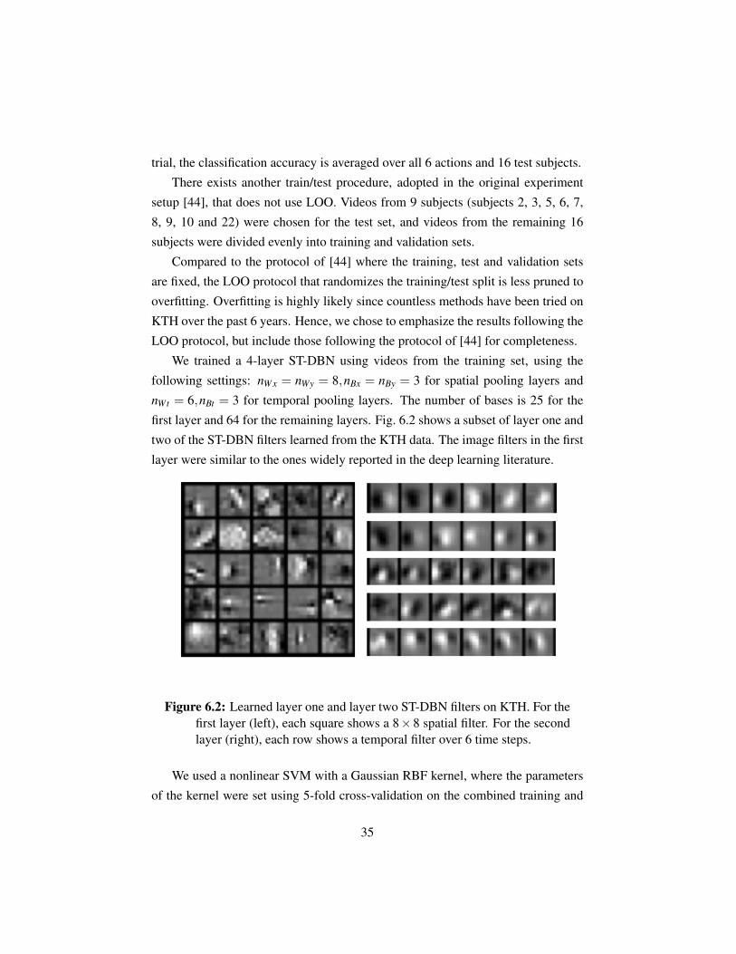
We trained a 4-layer ST-DBN using videos from the training set, using the

following settings: nWx = nWy = 8,nBx = nBy = 3 for spatial pooling layers and

nWt = 6,nBt = 3 for temporal pooling layers. The number of bases is 25 for the

first layer and 64 for the remaining layers. Fig. 6.2 shows a subset of layer one and

two of the ST-DBN filters learned from the KTH data. The image filters in the first

layer were similar to the ones widely reported in the deep learning literature.

Figure 6.2: Learned layer one and layer two ST-DBN filters on KTH. For thefirst layer (left), each square shows a 8×8 spatial filter. For the secondlayer (right), each row shows a temporal filter over 6 time steps.

We used a nonlinear SVM with a Gaussian RBF kernel, where the parameters

of the kernel were set using 5-fold cross-validation on the combined training and

35

validation set (similar to [26]). We compare the performance using outputs from

each layer of the STDBN. Since video lengths vary across the data samples, and

STDBN of different depth provides different degree of resolution reduction, the

output representations from the STDBN differ in size. Therefore, we reduce the

resolution of the output representation down to 4×5×6 via max-pooling.

6.2.2 Classification Performance

Table 6.1 shows classification results for both train/test protocols.

Table 6.1: Average classification accuracy results for KTH actions dataset.

LOO protocol Train/test protocol of [44]Method Accuracy (%) Method Accuracy (%)

4-layer ST-DBN 90.3 ± 0.83 4-layer ST-DBN 85.23-layer ST-DBN 91.13±0.85 3-layer ST-DBN 86.62-layer ST-DBN 89.73 ± 0.18 2-layer ST-DBN 84.61-layer ST-DBN 85.97 ± 0.94 1-layer ST-DBN 81.4

Liu and Shah [30] 94.2 Laptev et al. [26] 91.8Wang and Li [50] 87.8 Taylor et al. [46] 89.1Dollar et al. [11] 81.2 Schuldt et al. [44] 71.7

For the LOO protocol, classification results for a ST-DBN with up to 4 lay-

ers are shown, averaged over 4 trials. We included comparisons to three other

methods—all of which used an SVM classifier2. We see that having additional

(temporal and spatial) layers yields an improvement in performance, achieving a

competitive accuracy of 91% (for the 3rd layer). Interestingly, a 4th layer leads to

slightly worse classification accuracy. This can be attributed to excessive tempo-

ral pooling on an already short video snippet (around 100 frames long). The best

reported result to date, 94.2% by Liu and Shah [30], first used a bag-of-words ap-

proach on cuboid feature detectors and maximal mutual information to cluster the

video-words, and then boosted up performance by using hand-designed matching

2Dean et al. [8] report a classification accuracy of 81.1% under the LOO protocol. However,their result is not directly comparable to ours since they use a 1-NN classifier, instead of an SVMclassifier.

36

mechanisms to incorporate global spatio-temporal information. In contrast to their

work, we do not use feature detectors or matching mechanisms, and take the en-

tire video as input. Wang and Li [50] cropped the region of the video containing

the relevant activity and clustered difference frames. They also used a weighted

sequence descriptor that accounted for the temporal order of features.

For the train/test protocol of [44], we see a similar pattern in the performance

of ST-DBN as the number of layers increases. Laptev et al. [26] use a 3D Harris de-

tector, a HoG/HoF descriptor, and an SVM with a χ2 kernel. Taylor et al. [46] use

dense sampling of space-time cubes, along with a factored RBM model and sparse

coding to produce codewords that are then fed into an SVM classifier. Schuldt et

al. [44] use the space-time interest points of [25] and an SVM classifier.

6.2.3 Discussion

In table 6.1, the three-layered ST-DBN performs better than most methods using

the less overfitting-prone, LOO protocol, and achieves comparable accuracy in the

specific train/test split used by the protocol of [44].

Unlike the existing activity recognition methods, our model learns a feature

representation in a completely unsupervised manner. The model incorporates no

prior knowledge for the classification task apart from spatial and temporal smooth-

ness. Neither has the classification pipeline (the entire process that converts raw

videos into classification results) been tuned to improve the accuracy results. For

example, lower error rates could be achieved by adjusting the resolution of input

features to a SVM. Despite its fully unsupervised nature, our models achieves a

performance within 3% to 5% of the current state-of-the-art [26, 30], and a 10% to

15% reduction in error relative to the initial methods [11, 44] applied to KTH.

37

Chapter 7

ST-DBN as a Generative Model

In this chapter we present anecdotal results of video denoising and inferring miss-

ing portions of frames in a video sequence using a ST-DBN.

Note that same learned ST-DBN used for discrimination in chapter 6 is used

for the experiments of this chapter. To the best of our knowledge, the ST-DBN is

the only model capable of performing all these tasks within a single modeling

framework.

7.1 DenoisingWe denoise test videos from the KTH dataset using a one-layer and a two-layer

STDBN. For the two-layer STDBN, we first follow the procedure described in

Sec. 5.2 to generate the max-pooling units of the first layer, then we use Eqs. (5.4)

and (4.5) to generate high-resolution version of the data.

Fig. 7.1 shows denoising results. Fig. 7.1(a) shows the test frame, Fig. 7.1(b)

shows the noisy test frame, corrupted with additive Gaussian noise1, and Figs. 7.1(c)

and (d) show the reconstruction with a one-layer and a two-layer ST-DBN, respec-

tively. We see that the one-layer ST-DBN (Fig. 7.1(c)) denoises the image frame

well. The two-layer ST-DBN (with an additional temporal pooling layer) gives

slightly better background denoising. The normalized MSEs of one-layer and two-

layer reconstructions are 0.1751 and 0.155 respectively. For reference, the normal-

1Each pixel is corrupted with additive mean-zero Gaussian noise with a standard deviation of s,where s is the standard deviation of all pixels in the entire (clean) video.

38

ized MSE between the clean and noisy video has value 1. We include a link to the

denoised video in the supplementary material since the denoising effects are more

visible over time. Note that in Fig. 7.1, local contrast normalization was reversed to

visualize frames in the original image space, and image frames were downsampled

by a factor of 2 from the original KTH set.

Figure 7.1: Denoising results: (a) Test frame; (b) Test frame corrupted withnoise; (c) Reconstruction using 1-layer ST-DBN; (d) Reconstructionwith 2-layer ST-DBN.

7.2 PredictionFig. 7.2 illustrates the capacity of the ST-DBN to reconstruct data and generate

spatio-temportal predictions. The test video shows an observed sequence of gazes

in frames 2-4, where the focus of attention is on portions of the frame. The bottom

row of Fig. 7.2 shows the reconstructed data within the gaze window and predic-

tions outside this window.

The gazes are simulated by keeping a randomly sampled circular region for

39

each frame and zeroing out the rest. We use a three-layer STDBN and the same

reconstruction strategy as that in Sec. 7.1. In the reconstruction, for ease of visual-

ization, the region outside the gaze window are contrast enhanced to have the same

contrast as the region within.

Note that the blurry effect in prediction outside the gaze window is due to the

loss of information incurred with max-pooling. Though max-pooling comes at a

cost when inferring missing parts of frames, it is crucial for good discriminative

performance. Future research must address this fundamental trade-off. The re-

sults in the figure, though apparently simple, are quite remarkable. They represent

an important step toward the design of attentional mechanisms for gaze planning.

While gazing at the subject’s head, the model is able to infer where the legs are.

This coarse resolution gist may be used to guide the placement of high resolution

detectors.

Figure 7.2: Top video shows an observed sequence of gazes/foci of attention(i.e., frames 2-4). Bottom video shows reconstructions within the gazewindows and predictions outside them.

40

Chapter 8

Discussion and Conclusions

8.1 DiscussionThere remain a few avenues for discussion and future investigation.

• First, testing on larger video databases is an obvious immediate topic for

further research. Our model can be parallelized easily and to a high degree,

since the hidden representations are factorized. Future work will investigate

expediting training and inference with Graphical Processing Units.

• Interestingly, the max-pooling operation that allows feature invariance to be

captured hierarchically from spatio-temporal data has an adverse effect for

predicting missing parts of a video sequence due to loss of resolution. To

address this issue, future work will examine how to minimize the information

loss associated with max-pooling when performing inference. We conjecture

that combinations of models with and without pooling might be required.

• Additionally, samples from our model are produced by top-down informa-

tion only. Although treating our model as a Deep Boltzmann Machine and

using the corresponding sampling procedure incorporating both top-down

and bottom-up information, the fact that the model is trained as a Deep Be-

lief Network causes a double-counting problem in inference. Future work

should investigate efficient training of our model as a Deep Boltzmann Ma-

chine in order to perform sampling properly.

41

• Precautions should be taken to ensure representations are not made too com-

pact with too many layers in the architecture. Model selection is an open

challenge in this line of research.

• Finally, we plan to build on the gaze prediction results. Our intention is to

use planning to optimize the gaze locations so as to solve various recognition

and verification tasks efficiently.

8.2 ConclusionsIn this thesis, we introduced a hierarchical distributed probabilistic model for learn-

ing invariant features from spatio-temporal data. Using CRBMs as a building

block, our model, the Space-Time Deep Belief Network, pools over space and time.

It fulfills all the four desirable properties of a feature extractor that we reviewed in

the introduction. In addition to possessing feature invariance (for selectivity and

robustness to input transformations) and a hierarchical, distributed representation,

our model is generative and shows good discriminative performance on a simple

human action recognition task.

42

Bibliography

[1] M. M. A. Klaser and C. Schmid. A spatio-temporal descriptor based on3d-gradients. In BMVC, 2008. → pages 12

[2] R. Baddeley. Visual perception. An efficient code in v1? Nature, 1996. →pages 5

[3] S. Becker. Learning to categorize objects using temporal coherence. InNIPS, 1993. → pages 4

[4] Y. Bengio and Y. LeCun. Scaling learning algorithms towards AI. InLarge-Scale Kernel Machines. MIT Press, 2007. → pages 1, 4

[5] Y. Bengio, P. Lamblin, D. Popovici, and H. Larochelle. Greedy layer-wisetraining of deep networks. NIPS, 2006. → pages 2

[6] M. Booth and E. Rolls. View-invariant representations of familiar objects byneurons in the inferior temporal visual cortex. Cerebral Cortex, 1998. →pages 4

[7] C. Cadieu and B. A. Olshausen. Learning transformational invariants fromnatural movies. NIPS, 2008. → pages 7

[8] T. Dean, G. Corrado, and R. Washington. Recursive sparse, spatiotemporalcoding. IEEE International Symposium on Multimedia, 2009. → pages 1,12, 36

[9] G. Desjardins and Y. Bengio. Empirical evaluation of convolutional RBMsfor vision. Technical report, University of Montreal, 2008. → pages 2

[10] M. DeWeese, M. Wehr, and A. Zador. Binary spiking in auditory cortex.Journal of Neuroscience, 2003. → pages 5

[11] P. Dollar, V. Rabaud, G. Cottrell, and S. Belongie. Behavior recognition viasparse spatio-temporal features. VS-PETS, 2005. → pages 11, 36, 37

43

[12] L. Fei-Fei, R. Fergus, and P. Perona. Learning generative visual modelsfrom few training examples: an incremental Bayesian approach tested on101 object categories. CVPR, 2004. → pages 9

[13] P. Foldiak. Learning invariance from transformation sequences. NeuralComputation, 1991. → pages 4

[14] K. Fukushima. Neocognitron: a self-organizing neural network model for amechanism of pattern recognition unaffected by shift in position. BiologicalCybernetics, 1980. → pages 7

[15] I. Goodfellow, Q. Le, A. Saxe, and A. Ng. Measuring invariances in deepnetworks. NIPS, 2009. → pages 1, 31, 32

[16] J. Hawkins and D. George. Hierarchical temporal memory: Concepts,theory and terminology. Technical report, Numenta, 2006. → pages 2

[17] G. Hinton and T. Sejnowski. Unsupervised learning: Foundations of neuralcomputation. MIT Press, 1999. → pages 5

[18] G. Hinton, S. Osindero, and Y. Teh. A fast learning algorithm for deep beliefnets. Neural Comp., 2006. → pages 8, 27

[19] G. E. Hinton and R. R. Salakhutdinov. Reducing the dimensionality of datawith neural networks. Science, 2006. → pages 1, 2, 8, 23

[20] D. Hubel and T. Wiesel. Receptive fields, binocular interaction andfunctional architecture in the cat’s visual cortex. Journal of Physiology,1962. → pages 4, 6

[21] M. Ito, H. Tamura, I. Fujita, and K. Tanaka. Size and position invariance ofneural responses in monkey inferotemporal cortex. Journal ofNeurophysiology, 1995. → pages 4

[22] H. Jhuang, T. Serre, L. Wolf, and T. Poggio. A biologically inspired systemfor action recognition. In ICCV, 2007. → pages 11

[23] K. Kavukcuoglu, M. Ranzato, R. Fergus, and Y. LeCun. Learning invariantfeatures through topographic filter maps. CVPR, 2009. → pages 1

[24] A. Krizhevsky. Learning multiple layers of features from tiny images.Master’s thesis, University of Toronto, 2009. → pages 16

[25] I. Laptev and T. Lindeberg. Space-time interest points. ICCV, 2003. →pages 11, 37

44

[26] I. Laptev, M. Marszałek, C. Schmid, and B. Rozenfeld. Learning realistichuman actions from movies. CVPR, 2008. → pages 12, 36, 37

[27] Y. Lecun and Y. Bengio. Convolutional networks for images, speech, andtime-series. The handbook of brain theory and neural networks, 1998. →pages 7

[28] H. Lee, C. Ekanadham, and A. Ng. Sparse deep belief net model for visualarea V2. NIPS, 2008. → pages 9, 22

[29] H. Lee, R. Grosse, R. Ranganath, and A. Ng. Convolutional deep beliefnetworks for scalable unsupervised learning of hierarchical representations.ICML, 2009. → pages 1, 2, 21, 22, 23, 31

[30] J. Liu and M. Shah. Learning human action via information maximization.CVPR, 2008. → pages 36, 37

[31] B. Marlin, K. Swersky, B. Chen, and N. de Freitas. Inductive principles forrestricted boltzmann machine learning. In AISTATS, 2010. → pages 16

[32] R. Memisevic and G. E. Hinton. Learning to represent spatialtransformations with factored higher-order Boltzmann machines. NeuralComput., 2010. → pages 1

[33] H. Mobahi, R. Collobert, and J. Weston. Deep learning from temporalcoherence in video. ICML, 2009. → pages 1, 7

[34] V. Mountcastle. The columnar organization of the cerebral cortex. Brain,1997. → pages 4

[35] M. Norouzi, M. Ranjbar, and G. Mori. Stacks of convolutional restrictedBoltzmann machines for shift-invariant feature learning. CVPR, 2009. →pages 2, 9, 22, 23

[36] B. A. Olshausen and D. J. Field. Sparse coding with an overcomplete basisset: a strategy employed by v1? Vision Res, 1997. → pages 7

[37] M. Oram and D. Perrett. Modeling visual recognition from neurobiologicalconstraints. Neural Networks, 1994. → pages 4

[38] J. Perez-Orive, O. Mazor, G. Turner, S. Cassenaer, R. Wilson, andG. Larrent. Oscillations and sparsening of odor representations in themushroom body. Science, 2002. → pages 5

45

[39] R. Quiroga, L. Reddy, G. Kreiman, C. Koch, and I. Fried. Invariant visualrepresentation by single neurons in the human brain. Nature-Letters, 2005.→ pages 4

[40] M. Ranzato and G. Hinton. Modeling pixel means and covariances usingfactorized third-order boltzmann machines. In CVPR, 2010. → pages 9

[41] M.-A. Ranzato, F. J. Huang, Y.-L. Boureau, and Y. Lecun. Unsupervisedlearning of invariant feature hierarchies with applications to objectrecognition. In CVPR, 2007. → pages 2

[42] M. Riesenhuber and T. Poggio. Hierarchical models of object recognition incortex. Nature of Neuroscience, 1999. → pages 6

[43] R. Salakhutdinov and G. E. Hinton. Deep Boltzmann Machines. In ArtificialIntelligence and Statistics, 2009. → pages 9, 29

[44] C. Schuldt, I. Laptev, and B. Caputo. Recognizing human actions: A localSVM approach. ICPR, 2004. → pages 34, 35, 36, 37

[45] K. Swersky, B. Chen, B. Marlin, and N. de Freitas. A tutorial on stochasticapproximation algorithms for training restricted boltzmann machines anddeep belief nets. Information Theory and Applications Workshop, 2010. →pages 16

[46] G. W. Taylor and C. Bregler. Learning local spatio-temporal features foractivity recognition. Snowbird Learning Workshop, 2010. → pages 12, 36,37

[47] G. W. Taylor and G. E. Hinton. Factored conditional restricted Boltzmannmachines for modeling motion style. ICML, 2009. → pages 12

[48] K. Tsunoda, Y. Yamane, M. Nishizaki, and M. Tanifuji. Complex objects arerepresented in macaque inferotemporal cortex by the combination of featurecolumns. Nat. Neuroscience, 2001. → pages

[49] W. Vinje and J. Gallant. Sparse coding and decorrelation in primary visualcortex during natural vision. Science, 2000. → pages 5

[50] Z. Wang and B. Li. Human activity encoding and recognition usinglow-level visual features. IJCAI, 2009. → pages 34, 36, 37

[51] G. Willems, T. Tuytelarrs, and L. V. Gool. An efficient dense andscale-invariant spatio-temporal interest point detector. In ECCV, 2008. →pages 11

46

[52] L. Wiskott. How does our visual system achieve shift and size invariance?In J. van Hemmen and T. Sejnowski, editors, 23 Problems in SystemsNeuroscience. Oxford University Press, 2003. → pages 4

[53] L. Wiskott and T. J. Sejnowski. Slow feature analysis: Unsupervisedlearning of invariances. Neural Comput., 2002. → pages 1, 2, 4

[54] M. Zeiler, D.Kirshnan, G. Taylor, and R. Fergus. Deconvolutional networks.In CVPR, 2010. → pages 7

47