Deep Learning: Introduction

Vibhav Gogate

The University of Texas at Dallas

Motivation

• Look at our brains

• Many levels of processing

• Each level is learning features or representations at increasing level of abstraction

• Example: Model of visual cortex – Our brain first identifies edges, then patches,

surfaces, objects, etc. in that order

• Replicate this architecture = Deep Learning

Applications

• Computer Vision

• Speech

• Natural Language processing

• Video Processing (New???)

• Your own app here!

Deep models: Plenty of them

• Classification (does not work well) – Deep Multi-layer perceptrons

• Graphical models – Deep Directed networks (BNs)

– Deep Boltzmann Machines (Markov networks)

– Deep Belief Networks (BN+MN combination)

• Deep Auto-encoders

• Deep AND/OR graphs or Sum-product networks

Deep Directed Models • All CPDs are logistic

(Sigmoid networks)

• Inference is hard: Why?

– Correlated by explaining away

Slow inference; Slow learning

Deep Boltzmann machines • Inference is easier

– Block Gibbs sampling

• Learning is harder

– Partition function

• Greedy layer by layer learning works well in practice

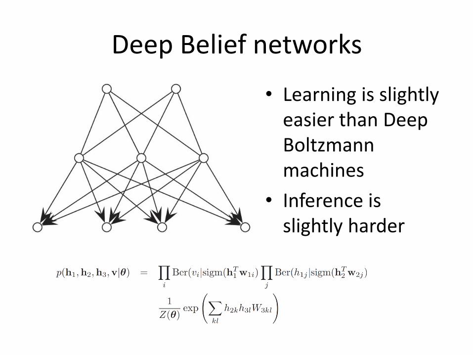
Deep Belief networks

• Learning is slightly easier than Deep Boltzmann machines

• Inference is slightly harder

Deep Auto-Encoder

• Auto-encoder: A neural network used for dimensionality reduction and feature discovery

– Trained to predict itself!

• Hidden layer is constrained to be a narrow bottleneck

– Otherwise, it will learn trivial identity mapping

• V->H->V

Deep Auto-Encoder

• Deep learning: Stack many layers E.g.: DBN [Hinton & Salakhutdinov, 2006]

CDBN [Lee et al., 2009]

DBM [Salakhutdinov & Hinton, 2010]

• Potentially much more powerful than shallow architectures [Bengio, 2009]

• But … – Inference is even harder

– Learning requires extensive effort

10

Sum-Product Networks: Motivation

10

11

Sum-Product Networks: Deep Tractable Models

Probability: P(X) = S(X) / Z

0.7 0.3

X1 X2

0.8 0.3 0.1 0.2 0.7 0.9 0.4

0.6

X1 X2

1 0 0 1

0.6 0.9 0.7 0.8

0.42 0.72

X: X1 = 1, X2 = 0

X1 1

X1 0

X2 0

X2 1

0.51

Applications: Handwritten Digit Classification using DBNs

• 3 layers

• Top layer is connected to 10 label units representing 10 digits (Hack!)

Applications: Handwritten Digit Classification using DBNs

• First two hidden layers were trained in a greedy unsupervised fashion using 30 passes over the data – Few hours

• Top layer trained using as input activations of the lower hidden layer as well as the class labels

• Weights Fine tuned using top-down procedure Errors

DBN: 1.25% SVM with degree 9 poly kernel: 1.4% 1-nearest neighbor: 3.1%

Applications: Handwritten Digit Classification using DBNs

Applications: Data visualization and feature discovery

• Learn informative features from raw data

• Use these features as input to supervised learning algorithms

2d visualization of some bag of words data from the Reuters RCV1-v2 corpus. Results of using a deep auto-encoder.

Applications: Learning Audio Features and Image Features

Applications: Learning Audio Features and Image Features

Filters learned in layers 2 and 3

18

Applications: Image Completion Sum-Product networks

SPN

DBN

Nearest Neighbor

DBM

PCA

Original

What we will cover?

• Architectures

– How many hidden layers to use?

– How many nodes in each hidden layer?

– Etc.

• Learning Algorithms

• Inference Algorithms

• Applications