Deep-Learning-Based Precipitation Observation Quality Control

Deep-Learning-Based Precipitation Observation Quality Control

YINGKAI SHA,a DAVID JOHN GAGNE II,b GREGORY WEST,c AND ROLAND STULLa

aThe University of British Columbia, Vancouver, British Columbia, CanadabNational Center for Atmospheric Research, Boulder, Colorado

cBC Hydro, Burnaby, British Columbia, Canada

(Manuscript received 1 June 2020, in final form 18 February 2021)

ABSTRACT: We present a novel approach for the automated quality control (QC) of precipitation for a sparse station

observation network within the complex terrain of British Columbia, Canada. Our QC approach uses convolutional neural

networks (CNNs) to classify bad observation values, incorporating a multiclassifier ensemble to achieve better QC per-

formance. We train CNNs using human QC’d labels from 2016 to 2017 with gridded precipitation and elevation analyses as

inputs. Based on the classification evaluation metrics, our QC approach shows reliable and robust performance across

different geographical environments (e.g., coastal and inland mountains), with 0.927 area under curve (AUC) and type

I/type II error lower than 15%. Based on the saliency-map-based interpretation studies, we explain the success of CNN-

based QC by showing that it can capture the precipitation patterns around, and upstream of the station locations.

This automated QC approach is an option for eliminating bad observations for various applications, including the pre-

processing of training datasets for machine learning. It can be used in conjunction with human QC to improve upon what

could be accomplished with either method alone.

KEYWORDS: Precipitation; Data quality control; Classification; Deep learning; Machine learning

1. Introduction

Precipitation observation quality control (QC) is a long-

standing challenge because of its high spatial and temporal

variability with skewed intensity spectra: the majority of pre-

cipitation observations are close to zero; while rare extreme

events can bring abnormally high precipitation values that

behave similarly to spurious outliers. On the instrumental side,

gauge-based precipitation measurements are biased by both

systematic instrumental errors (e.g., splashing/blowing of

rain/snow in/out of the gauge, losses due to the aerody-

namic effects above the gauge orifice, water adhering to

the gauge surface and evaporation) (Goodison et al. 1998;

Adam and Lettenmaier 2003; Yang et al. 2005; Rasmussen

et al. 2012), and technical or maintenance issues (e.g.,

mechanical malfunctions, data transmission error; Groisman

and Legates 1994).

Sophisticated QC procedures have been carried out in var-

ious meteorological and hydrological research projects. These

QC procedures are typically a mix of automated examination

of internal consistencies (i.e., checks of value range, rate of

change, and homogeneity with predefined thresholds) (Meek

and Hatfield 1994; Eischeid et al. 2000; Adler et al. 2003;

Schneider et al. 2014) and human-based QC with graphical

workstations (i.e., displaying precipitation values together with

orography and other background fields to determine their

quality) (e.g., Xie and Arkin 1996; Jørgensen et al. 1998; Adler

et al. 2003; Schneider et al. 2014). Although human-involved

QC has reported success in many projects, this approach is

resource-intensive and can cause delays when processing a

high volume of data (Mourad and Bertrand-Krajewski 2002).

Human QC may also bring subjectivity into the quality labels,

resulting in a downgrade of data quality.

Many automated observation QC methods have been pro-

posed to reduce the workload of human-based QC, including

1) time series-based anomaly detection (e.g., Mourad and

Bertrand-Krajewski 2002; Piatyszek et al. 2000; You et al.

2007), 2) cross validating neighboring stations with geo-

statistical methods (e.g., Eischeid et al. 1995; Hubbard et al.

2005; �St�epánek et al. 2009; Xu et al. 2014), and 3) bad-value

classification with decision trees (e.g., Martinaitis et al. 2015; Qi

et al. 2016) and neural networks (Sciuto et al. 2009; Lakshmanan

et al. 2007, 2014; Zhao et al. 2018).

In this study, we provide a novel automated QC approach

for precipitation observations with deep artificial neural net-

works (DNNs). We define automated QC as a binary classifi-

cation problem—that is, classifying each observation with a

‘‘good’’ or ‘‘bad’’ QC flag. The type of DNN applied in this

study is a convolutional neural network (CNN). Our CNNs

take station precipitation observations, preprocessed gridded

precipitation and elevation values centered around each sta-

tion location as inputs, using human-labeled quality flags as

training targets.

Based on the ability of CNNs to learn from gridded data, in

this study, we aim to provide an automated QC method that

requires less data dependencies. As we will introduce later, this

research focuses on gauge data from a specific observation

network; however, the potential of generalization and data

dependency replacements are also discussed. This is in contrast

to many existing QCmethods that require a greater number of

Denotes content that is immediately available upon publica-

tion as open access.

Corresponding author: Yingkai Sha, [email protected]

MAY 2021 SHA ET AL . 1075

DOI: 10.1175/JTECH-D-20-0081.1

� 2021 American Meteorological Society. For information regarding reuse of this content and general copyright information, consult the AMS CopyrightPolicy (www.ametsoc.org/PUBSReuseLicenses).

Brought to you by University of Colorado Libraries | Unauthenticated | Downloaded 07/27/21 11:11 PM UTC

mailto:[email protected]

http://www.ametsoc.org/PUBSReuseLicenses



observational data sources and/or ones with greater spatial

coverage [e.g., closely located neighboring stations (Maul-

Kötter and Einfalt 1998), radar coverage (Martinaitis et al.

2015; Qi et al. 2016)].

Based on the above concepts, we apply the following hy-

potheses in this research: CNNs are capable of 1) learning

representations of precipitation patterns from gridded pre-

cipitation input, 2) learning representations of complex terrain

conditions from gridded elevation input, and 3) utilizing these

representations to classify QC flags. Further, with the above

research hypotheses, we address the following research ques-

tions: 1) How well can CNNs classify QC flags? 2) What is the

role of elevation input in this QC problem? 3) Given the im-

perfection of gridded precipitation analysis, can we preprocess

this input to enable CNNs to learn effective representations?

And 4) can we explain the classification behavior of CNNs in

this QC problem?

The rest of this paper is organized as follows: section 2 de-

scribes the region of interest and data; section 3 introduces

methodologies, including the design of CNNs and the auto-

mated QC workflows; section 4 evaluates the general classifi-

cation results and answers research questions 1 and 2; section 5

provides interpretation studies of CNNs and answers research

questions 3 and 4; and sections 6 and 7 are the discussion and

conclusions.

2. Data

a. Region of interest

The region of interest for this research is British Columbia

(BC), Canada. BC is located in southwestern Canada, bor-

dering the northeast Pacific Ocean and has complex geo-

graphical conditions. The south coast of BC is a combination of

coastal and mountainous environments. Southeastern BC is

covered by the Columbia and Rocky Mountains, whereas

central and northeastern BC are a mix of flat terrain and

mountain ranges (Odon et al. 2018).

Precipitation observation QC is complicated in BC by its

complex terrain, which negatively impacts the continuity,

reliability, and spatial representativeness of ground-based

observations (Banta et al. 2013). Good-quality observations

are needed in numerical weather prediction (NWP) opera-

tions for postprocessing, verifying, and analyzing the fore-

cast. Excluding bad gauge values to preserve the quality of

precipitation observations within BC watersheds is of spe-

cial importance as hydrology models are sensitive to the

station precipitation inputs (e.g., Nearing et al. 2005; Null

et al. 2010). Small changes in precipitation can cause large

changes in watershed response. Good-quality precipitation

observations are fundamental to correctly estimating the

hydrological states of these watersheds and to postprocess

precipitation forecast inputs.

The main electric utility in BC, BC Hydro, generates more

than 90% of its electricity from hydropower, mostly within the

watersheds of the Peace (northeastern BC) and Columbia

(southeastern BC) River basins (BC Hydro 2020). Reliable

hydrological forecasts are critical to the planning and opera-

tion of these hydroelectric facilities. Greater automation of the

QC process would offer more timely and reliable and less

resource-intensive precipitation data in support of this.

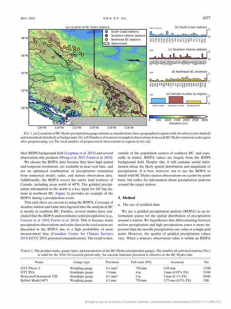
b. In situ observations

The in situ observations applied in this research are taken

from 80 gauge stations within and near BC Hydro watersheds

(Fig. 1a). We divide these watersheds into three regions based

on their precipitation regimes: 1) the south coast, directly af-

fected by Pacific frontal cyclone systems in the wet fall, winter,

and spring months, with dry summer months (Fig. 1a, blue

dots); 2) the southern interior, which sees frequent, but lighter

precipitation amounts year-round (Fig. 1a, red dots); and 3)

northeast BC, which sees drier winters and wetter summers

(Fig. 1a, yellow dots) (e.g., Chilton 1981; Odon et al. 2018).

BCHydro stations use standpipe- and weighing-bucket-type

precipitation gauges; they provide real-time gauge observa-

tions as heights with accuracies ranging from 2.0 to 0.05mm,

reporting precisions ranging from 0.1 to 1.0mm and reporting

intervals varying from every 15min to every 2 h (Table 1; BC

Hydro 2019, personal communication). A given station can

have different precision and observation frequencies at

different times in its period of record. Manual (human) QC

is performed on the raw gauge observations with the fol-

lowing steps: 1) Precipitation trends are compared against

nearby stations known to have similar precipitation pat-

terns. 2) Precipitation amounts are compared with the

Regional Deterministic Precipitation Analysis (described in

the following subsection) and with collocated snow pillows.

3) When in doubt, BC Hydro Meteorologists are consulted

(BC Hydro 2019, personal communication). Although not

perfect, these human QC’d observations are recognized as

reliable values in this research, and are used to create

quality labels for the supervised training of the automated

QC system.

c. Gridded data

We use two gridded datasets: elevation obtained fromETOPO1

(Amante and Eakins 2009) and accumulated 6-h precipita-

tion obtained from the Canadian Regional Deterministic

Precipitation Analysis (RDPA).

ETOPO1 is a 1-arc-min resolution global elevation model

maintained by theNationalGeophysical DataCenter. ETOPO1

elevation is a key input of ourmethod because orography largely

controls the distribution of precipitation over BC.

The Canadian Meteorological Centre (CMC) within

Environment and Climate Change Canada (ECCC) produces

the Canadian Precipitation Analysis (CaPA), comprised of

the Regional and High Resolution Deterministic Precipitation

Analyses (RDPAandHRDPA, respectively) (CanadianCentre

for Climate Services 2019). The RDPA, used in this study, takes

the output of the 10-km Regional Deterministic Prediction

System (RDPS) as its background field and has been calibrated

with radar products from Canadian Weather Radar Network,

and with gauge observations from multiple observational net-

works (BC Hydro observations are not ingested) through opti-

mum interpolation (OI) (Mahfouf et al. 2007; Fortin et al. 2015).

The RDPA data exhibit generally good and homogeneous skill

throughout Canada (Lespinas et al. 2015). They outperform

1076 JOURNAL OF ATMOSPHER IC AND OCEAN IC TECHNOLOGY VOLUME 38


their RDPS background field (Lespinas et al. 2015) and several

observation only products (Wong et al. 2017; Fortin et al. 2018).

We choose the RDPA data because they have high spatial

and temporal resolutions, are available in near–real time, and

are an optimized combination of precipitation estimation

from numerical model, radar, and station observation data.

Additionally, the RDPA covers the entire land territory of

Canada, including areas north of 608N. The gridded precipi-

tation information in the north is a key input for QC’ing sta-

tions in northeast BC. Figure 2a provides an example of the

RDPA during a precipitation event.

That said, there are caveats to using the RDPA. Coverage of

weather-station and radar data ingested into the analysis in BC

is mostly in southern BC. Further, several studies have con-

cluded that the RDPA underestimates solid precipitation (e.g.,

Carrera et al. 2010; Fortin et al. 2018). This is because many

precipitation observations and radar data in the cool season are

discarded in the RDPA due to a high probability of snow

measurement bias (Canadian Centre for Climate Services

2019; ECCC 2019, personal communication). The result is that,

outside of the population centers of southern BC, and espe-

cially in winter, RDPA values are largely from the RDPS

background field. Despite this, it still contains useful infor-

mation about the likely spatial distribution and magnitude of

precipitation. It is best, however, not to use the RDPA to

match with BCHydro station observations on a point-by-point

basis, but rather for information about precipitation patterns

around the target station.

3. Method

a. The use of gridded data

We use a gridded precipitation analysis (RDPA) as an in-

formation source for the spatial distribution of precipitation

around a station. We hypothesize that differentiating between

no/low precipitation and high precipitation zones is more im-

portant than the specific precipitation rate value at a single grid

point. However, the quality of gridded precipitation values

vary. When a nonzero observation value is within an RDPA

FIG. 1. (a) Locations of BCHydro precipitation gauge stations as classified into three geographical regions with elevation (color shaded)

andwatersheds (hatched) as background. (b)–(d)Numbers of nonzero resampled observations from eachBCHydro station in each region

after preprocessing. (e) The total number of preprocessed observations in regions in (b)–(d).

TABLE 1. The product name, gauge types, and parameters of the BC Hydro precipitation gauges. The number of activated stations (No.)

is valid for the 2016–18 research period only. An asterisk indicates precision is effective at the BC Hydro side.

Name Gauge type Precision Full scale (FS) Accuracy No.

OTT Pluvio 2 Weighing gauge 0.1 mm* 750mm 0.05mm 15/80

OTT PLS Standpipe gauge 1.0mm 4m 2mm (0.05% FS) 33/80

Honeywell Sensotech TJE Standpipe gauge 0.1 mm* 2m 2mm (0.1% FS) 30/80

Belfort Model 6071 Weighing gauge 0.1mm 750mm 3.75mm (0.5% FS) 2/80



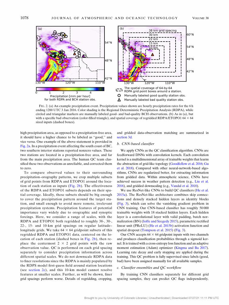
high precipitation area, as opposed to a precipitation-free area,

it should have a higher chance to be labeled as ‘‘good,’’ and

vice versa. One example of the above statement is provided in

Fig. 2a. In a precipitation event affecting the south coast of BC,

two southern interior stations reported nonzero values. These

two stations are located in a precipitation-free area, and far

from the main precipitation area. The human QC team clas-

sified these two observations as unreliable, and corrected them

to zero.

To compare observed values to their surrounding

precipitation–orography patterns, we crop multiple subsets

of grid points from RDPA and ETOPO1 around the loca-

tion of each station as inputs (Fig. 2b). The effectiveness

of the RDPA and ETOPO1 subsets depends on their spa-

tial coverage. Ideally, these subsets should be big enough

to cover the precipitation pattern around the target sta-

tion, and small enough to avoid more remote, irrelevant

precipitation systems. Precipitation features of potential

importance vary widely due to orographic and synoptic

forcings. Here, we consider a range of scales, with the

RDPA and ETOPO1 both regridded to roughly 38-, 30-,

22-, 15- and 10-km grid spacings on regular latitude–

longitude grids. We take 64 3 64 gridpoint subsets of this

regridded RDPA and ETOPO1 data, centered on the lo-

cation of each station (dashed boxes in Fig. 2b), then re-

place the centermost 2 3 2 grid points with the raw

observation value. QC is performed on each grid spacing

separately to consider precipitation information across

different spatial scales. We do not downscale RDPA data

to finer resolutions since the RDPA is mainly populated by

the RDPS model first-guess field around station locations

(see section 2c), and this 10-km model cannot resolve

features at smaller scales. Further, as will be shown, finer

grid spacings perform worse. Details of regridding, cropping,

and gridded data-observation matching are summarized in

section 3d.

b. CNN-based classifier

We apply CNNs as the QC classification algorithm. CNNs are

feedforward DNNs with convolution kernels. Each convolution

kernel is amultidimensional array of trainable weights that learns

the abstraction of grid-like topology (Goodfellow et al. 2016; Gu

et al. 2018). Compared with other neural-network-based algo-

rithms, CNNs are regularized better, for extracting information

from gridded data. Within atmospheric science, CNNs have

achieved success in weather pattern detection (e.g., Liu et al.

2016), and gridded downscaling (e.g., Vandal et al. 2018).

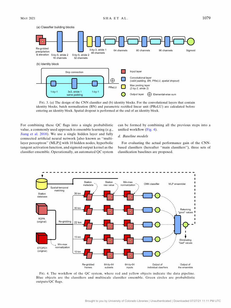
We use ResNet-like CNNs to build QC classifiers (He et al.

2015a). The ResNet-like architecture combines skip connec-

tions and densely stacked hidden layers as identity blocks

(Fig. 3), which can solve the vanishing gradient problem in

CNN training. Our CNN-based classifier has roughly 50 000

trainable weights with 18 stacked hidden layers. Each hidden

layer is a convolutional layer with valid padding, batch nor-

malization (BN) (Ioffe and Szegedy 2015), parametric rectified

linear unit (PReLU) (He et al. 2015b) activation function and

spatial dropout (Tompson et al. 2015) (Fig. 3).

Our CNN accepts 643 64 gridpoint inputs with two channels

and produces classification probabilities through a sigmoid ker-

nel. It is trainedwith a cross-entropy loss function and an adaptive

moment estimation (Adam) optimizer (Kingma and Ba 2017).

Learning rate decay and early stopping are applied during the

training. This QC problem is fully supervised since labels (good,

bad) have been assigned manually for all available samples.

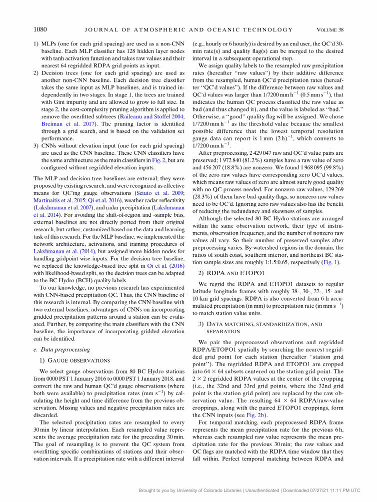
c. Classifier ensembles and QC workflow

By training CNN classifiers separately for different grid

spacing samples, they can predict QC flags independently.

FIG. 2. (a) An example precipitation event. Precipitation values shown are hourly precipitation rates for the 6 h

ending 1200 UTC 3 Jan 2016. Color shading is the Regional Deterministic Precipitation Analysis (RDPA), while

circled and triangular markers are manually labeled good- and bad-quality BCH observations. (b) As in (a), but

with a specific bad observation (color-filled triangle), and spatial coverage of regridded RDPA/ETOPO1 64 3 64

sized inputs (dashed boxes).



For combining these QC flags into a single probabilistic

value, a commonly used approach is ensemble learning (e.g.,

Jiang et al. 2018). We use a single hidden layer and fully

connected artificial neural network [also known as ‘‘multi-

layer perceptron’’ (MLP)] with 10 hidden nodes, hyperbolic

tangent activation function, and sigmoid output kernel as the

classifier ensemble. Operationally, an automated QC system

can be formed by combining all the previous steps into a

unified workflow (Fig. 4).

d. Baseline models

For evaluating the actual performance gain of the CNN-

based classifiers (hereafter ‘‘main classifiers’’), three sets of

classification baselines are proposed.

FIG. 3. (a) The design of the CNN classifier and (b) identity blocks. For the convolutional layers that contain

identity blocks, batch normalization (BN) and parametric rectified linear unit (PReLU) are calculated before

entering an identity block. Spatial dropout is performed at the end of an identity block.

FIG. 4. The workflow of the QC system, where red and yellow objects indicate the data pipeline.

Blue objects are the classifiers and multiscale classifier ensemble. Green circles are probabilistic

outputs/QC flags.



1) MLPs (one for each grid spacing) are used as a non-CNN

baseline. Each MLP classifier has 128 hidden layer nodes

with tanh activation function and takes raw values and their

nearest 64 regridded RDPA grid points as input.

2) Decision trees (one for each grid spacing) are used as

another non-CNN baseline. Each decision tree classifier

takes the same input as MLP baselines, and is trained in-

dependently in two stages. In stage 1, the trees are trained

with Gini impurity and are allowed to grow to full size. In

stage 2, the cost-complexity pruning algorithm is applied to

remove the overfitted subtrees (Raileanu and Stoffel 2004;

Breiman et al. 2017). The pruning factor is identified

through a grid search, and is based on the validation set

performance.

3) CNNs without elevation input (one for each grid spacing)

are used as the CNN baseline. These CNN classifiers have

the same architecture as themain classifiers in Fig. 2, but are

configured without regridded elevation inputs.

The MLP and decision tree baselines are external; they were

proposed by existing research, andwere recognized as effective

means for QC’ing gauge observations (Sciuto et al. 2009;

Martinaitis et al. 2015; Qi et al. 2016), weather radar reflectivity

(Lakshmanan et al. 2007), and radar precipitation (Lakshmanan

et al. 2014). For avoiding the shift-of-region and -sample bias,

external baselines are not directly ported from their original

research, but rather, customized based on the data and learning

task of this research. For theMLP baseline, we implemented the

network architecture, activations, and training procedures of

Lakshmanan et al. (2014), but assigned more hidden nodes for

handling gridpoint-wise inputs. For the decision tree baseline,

we replaced the knowledge-based tree split in Qi et al. (2016)

with likelihood-based split, so the decision trees can be adapted

to the BC Hydro (BCH) quality labels.

To our knowledge, no previous research has experimented

with CNN-based precipitation QC. Thus, the CNN baseline of

this research is internal. By comparing the CNN baseline with

two external baselines, advantages of CNNs on incorporating

gridded precipitation patterns around a station can be evalu-

ated. Further, by comparing the main classifiers with the CNN

baseline, the importance of incorporating gridded elevation

can be identified.

e. Data preprocessing

1) GAUGE OBSERVATIONS

We select gauge observations from 80 BC Hydro stations

from 0000 PST 1 January 2016 to 0000 PST 1 January 2018, and

convert the raw and human QC’d gauge observations (where

both were available) to precipitation rates (mm s21) by cal-

culating the height and time difference from the previous ob-

servation. Missing values and negative precipitation rates are

discarded.

The selected precipitation rates are resampled to every

30min by linear interpolation. Each resampled value repre-

sents the average precipitation rate for the preceding 30min.

The goal of resampling is to prevent the QC system from

overfitting specific combinations of stations and their obser-

vation intervals. If a precipitation rate with a different interval

(e.g., hourly or 6 hourly) is desired by an end user, theQC’d 30-

min rate(s) and quality flag(s) can be merged to the desired

interval in a subsequent operational step.

We assign quality labels to the resampled raw precipitation

rates (hereafter ‘‘raw values’’) by their additive difference

from the resampled, human QC’d precipitation rates (hereaf-

ter ‘‘QC’d values’’). If the difference between raw values and

QC’d values was larger than 1/7200mmh21 (0.5mm s21), that

indicates the human QC process classified the raw value as

bad (and thus changed it), and the value is labeled as ‘‘bad.’’

Otherwise, a ‘‘good’’ quality flag will be assigned. We chose

1/7200 mm h21 as the threshold value because the smallest

possible difference that the lowest temporal resolution

gauge data can report is 1 mm (2 h)21, which converts to

1/7200 mm h21.

After preprocessing, 2 429 047 raw and QC’d value pairs are

preserved; 1 972 840 (81.2%) samples have a raw value of zero

and 456 207 (18.8%) are nonzero. We found 1 968 095 (99.8%)

of the zero raw values have corresponding zero QC’d values,

which means raw values of zero are almost surely good quality

with no QC process needed. For nonzero raw values, 129 269

(28.3%) of them have bad-quality flags, so nonzero raw values

need to be QC’d. Ignoring zero raw values also has the benefit

of reducing the redundancy and skewness of samples.

Although the selected 80 BC Hydro stations are arranged

within the same observation network, their type of instru-

ments, observation frequency, and the number of nonzero raw

values all vary. So their number of preserved samples after

preprocessing varies. By watershed regions in the domain, the

ratios of south coast, southern interior, and northeast BC sta-

tion sample sizes are roughly 1:1.5:0.65, respectively (Fig. 1).

2) RDPA AND ETOPO1

We regrid the RDPA and ETOPO1 datasets to regular

latitude–longitude frames with roughly 38-, 30-, 22-, 15- and

10-km grid spacings. RDPA is also converted from 6-h accu-

mulated precipitation (inmm) to precipitation rate (inmm s21)

to match station value units.

3) DATA MATCHING, STANDARDIZATION, AND

SEPARATION

We pair the preprocessed observations and regridded

RDPA/ETOPO1 spatially by searching the nearest regrid-

ded grid point for each station (hereafter ‘‘station grid

point’’). The regridded RDPA and ETOPO1 are cropped

into 64 3 64 subsets centered on the station grid point. The

2 3 2 regridded RDPA values at the center of the cropping

(i.e., the 32nd and 33rd grid points, where the 32nd grid

point is the station grid point) are replaced by the raw ob-

servation value. The resulting 64 3 64 RDPA/raw-value

croppings, along with the paired ETOPO1 croppings, form

the CNN inputs (see Fig. 2b).

For temporal matching, each preprocessed RDPA frame

represents the mean precipitation rate for the previous 6 h,

whereas each resampled raw value represents the mean pre-

cipitation rate for the previous 30min; the raw values and

QC flags are matched with the RDPA time window that they

fall within. Perfect temporal matching between RDPA and



observations is not needed because we are not performing

point-to-point comparisons (see section 3a), and is impossible

because of their frequency difference.

All datasets are standardized through minimum-maximum

normalization. The precipitation input croppings are normal-

ized independently to avoid the strong fluctuations of scales

across dry and rainy seasons.

We use 2016 data for training; and data in 2017 within 15-day

continuous periods starting at a random day of February,

April, June, October for validation; and the rest of the 2017

data for testing. Training and validation data are split into

balanced batches with each batch containing 100 bad raw value

samples and 100 good raw value samples (i.e., a balanced batch

size of 200). Testing data are grouped separately for evalua-

tions. They contain 6700 bad and 24 060 good raw value sam-

ples, respectively. Note that missing RDPA data and the

rounding of a fixed batch size will discard a small part of the

preprocessed data.

4. Results

a. Classification verification metrics

We assign the ‘‘good’’ quality for a given observation as the

true null hypothesis, or the ‘‘negative class,’’ because the ma-

jority of observations are of good quality; vice versa for ‘‘bad’’

quality and the ‘‘positive class.’’

We do not use regular categorical weather forecast verifi-

cation metrics because many of them are positively oriented,

which ignores the importance of accepting/rejecting the true

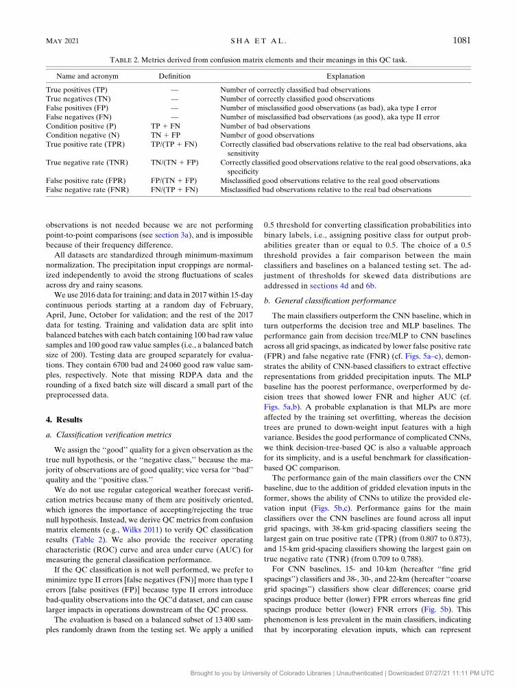
null hypothesis. Instead, we derive QC metrics from confusion

matrix elements (e.g., Wilks 2011) to verify QC classification

results (Table 2). We also provide the receiver operating

characteristic (ROC) curve and area under curve (AUC) for

measuring the general classification performance.

If the QC classification is not well performed, we prefer to

minimize type II errors [false negatives (FN)] more than type I

errors [false positives (FP)] because type II errors introduce

bad-quality observations into the QC’d dataset, and can cause

larger impacts in operations downstream of the QC process.

The evaluation is based on a balanced subset of 13 400 sam-

ples randomly drawn from the testing set. We apply a unified

0.5 threshold for converting classification probabilities into

binary labels, i.e., assigning positive class for output prob-

abilities greater than or equal to 0.5. The choice of a 0.5

threshold provides a fair comparison between the main

classifiers and baselines on a balanced testing set. The ad-

justment of thresholds for skewed data distributions are

addressed in sections 4d and 6b.

b. General classification performance

The main classifiers outperform the CNN baseline, which in

turn outperforms the decision tree and MLP baselines. The

performance gain from decision tree/MLP to CNN baselines

across all grid spacings, as indicated by lower false positive rate

(FPR) and false negative rate (FNR) (cf. Figs. 5a–c), demon-

strates the ability of CNN-based classifiers to extract effective

representations from gridded precipitation inputs. The MLP

baseline has the poorest performance, overperformed by de-

cision trees that showed lower FNR and higher AUC (cf.

Figs. 5a,b). A probable explanation is that MLPs are more

affected by the training set overfitting, whereas the decision

trees are pruned to down-weight input features with a high

variance. Besides the good performance of complicated CNNs,

we think decision-tree-based QC is also a valuable approach

for its simplicity, and is a useful benchmark for classification-

based QC comparison.

The performance gain of the main classifiers over the CNN

baseline, due to the addition of gridded elevation inputs in the

former, shows the ability of CNNs to utilize the provided ele-

vation input (Figs. 5b,c). Performance gains for the main

classifiers over the CNN baselines are found across all input

grid spacings, with 38-km grid-spacing classifiers seeing the

largest gain on true positive rate (TPR) (from 0.807 to 0.873),

and 15-km grid-spacing classifiers showing the largest gain on

true negative rate (TNR) (from 0.709 to 0.788).

For CNN baselines, 15- and 10-km (hereafter ‘‘fine grid

spacings’’) classifiers and 38-, 30-, and 22-km (hereafter ‘‘coarse

grid spacings’’) classifiers show clear differences; coarse grid

spacings produce better (lower) FPR errors whereas fine grid

spacings produce better (lower) FNR errors (Fig. 5b). This

phenomenon is less prevalent in the main classifiers, indicating

that by incorporating elevation inputs, which can represent

TABLE 2. Metrics derived from confusion matrix elements and their meanings in this QC task.

Name and acronym Definition Explanation

True positives (TP) — Number of correctly classified bad observations

True negatives (TN) — Number of correctly classified good observations

False positives (FP) — Number of misclassified good observations (as bad), aka type I error

False negatives (FN) — Number of misclassified bad observations (as good), aka type II error

Condition positive (P) TP 1 FN Number of bad observations

Condition negative (N) TN 1 FP Number of good observations

True positive rate (TPR) TP/(TP 1 FN) Correctly classified bad observations relative to the real bad observations, aka

sensitivity

True negative rate (TNR) TN/(TN 1 FP) Correctly classified good observations relative to the real good observations, aka

specificity

False positive rate (FPR) FP/(TN 1 FP) Misclassified good observations relative to the real good observations

False negative rate (FNR) FN/(TP 1 FN) Misclassified bad observations relative to the real bad observations



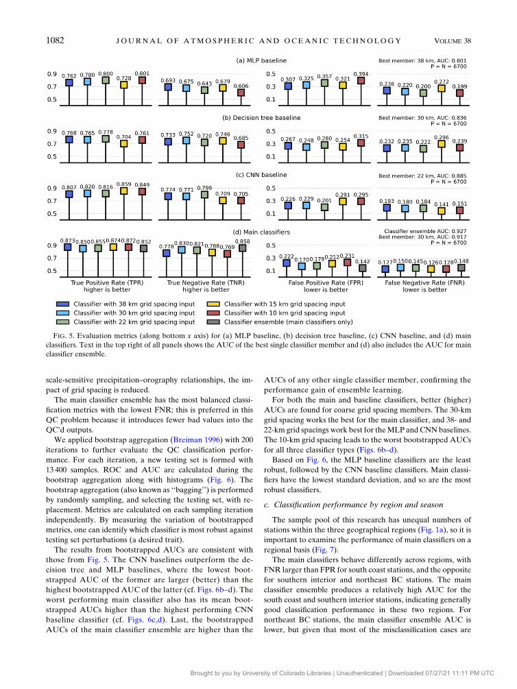
scale-sensitive precipitation–orography relationships, the im-

pact of grid spacing is reduced.

The main classifier ensemble has the most balanced classi-

fication metrics with the lowest FNR; this is preferred in this

QC problem because it introduces fewer bad values into the

QC’d outputs.

We applied bootstrap aggregation (Breiman 1996) with 200

iterations to further evaluate the QC classification perfor-

mance. For each iteration, a new testing set is formed with

13 400 samples. ROC and AUC are calculated during the

bootstrap aggregation along with histograms (Fig. 6). The

bootstrap aggregation (also known as ‘‘bagging’’) is performed

by randomly sampling, and selecting the testing set, with re-

placement. Metrics are calculated on each sampling iteration

independently. By measuring the variation of bootstrapped

metrics, one can identify which classifier is most robust against

testing set perturbations (a desired trait).

The results from bootstrapped AUCs are consistent with

those from Fig. 5. The CNN baselines outperform the de-

cision tree and MLP baselines, where the lowest boot-

strapped AUC of the former are larger (better) than the

highest bootstrapped AUC of the latter (cf. Figs. 6b–d). The

worst performing main classifier also has its mean boot-

strapped AUCs higher than the highest performing CNN

baseline classifier (cf. Figs. 6c,d). Last, the bootstrapped

AUCs of the main classifier ensemble are higher than the

AUCs of any other single classifier member, confirming the

performance gain of ensemble learning.

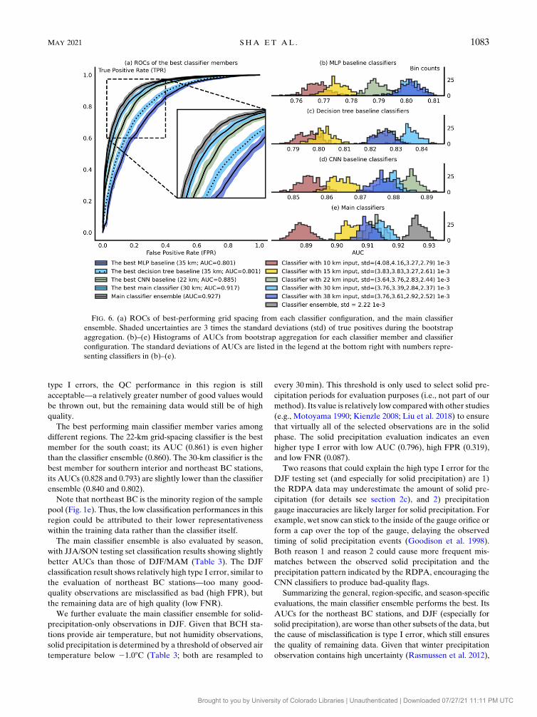
For both the main and baseline classifiers, better (higher)

AUCs are found for coarse grid spacing members. The 30-km

grid spacing works the best for the main classifier, and 38- and

22-km grid spacings work best for theMLP andCNNbaselines.

The 10-km grid spacing leads to the worst bootstrapped AUCs

for all three classifier types (Figs. 6b–d).

Based on Fig. 6, the MLP baseline classifiers are the least

robust, followed by the CNN baseline classifiers. Main classi-

fiers have the lowest standard deviation, and so are the most

robust classifiers.

c. Classification performance by region and season

The sample pool of this research has unequal numbers of

stations within the three geographical regions (Fig. 1a), so it is

important to examine the performance of main classifiers on a

regional basis (Fig. 7).

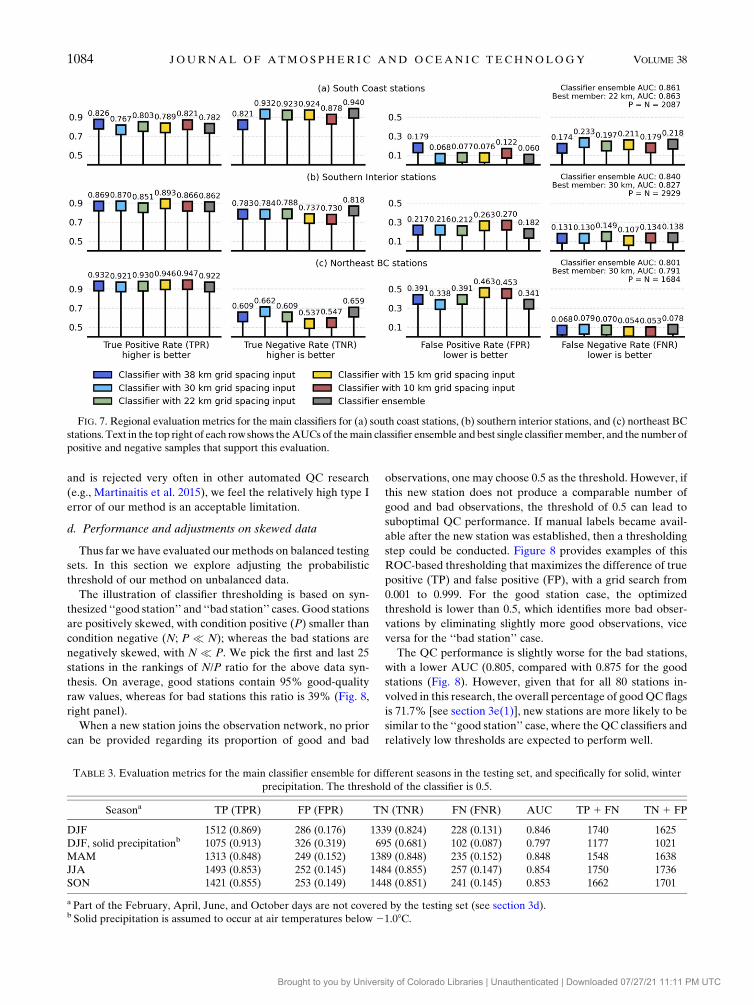
The main classifiers behave differently across regions, with

FNR larger than FPR for south coast stations, and the opposite

for southern interior and northeast BC stations. The main

classifier ensemble produces a relatively high AUC for the

south coast and southern interior stations, indicating generally

good classification performance in these two regions. For

northeast BC stations, the main classifier ensemble AUC is

lower, but given that most of the misclassification cases are

FIG. 5. Evaluation metrics (along bottom x axis) for (a) MLP baseline, (b) decision tree baseline, (c) CNN baseline, and (d) main

classifiers. Text in the top right of all panels shows the AUC of the best single classifier member and (d) also includes the AUC for main

classifier ensemble.



type I errors, the QC performance in this region is still

acceptable—a relatively greater number of good values would

be thrown out, but the remaining data would still be of high

quality.

The best performing main classifier member varies among

different regions. The 22-km grid-spacing classifier is the best

member for the south coast; its AUC (0.861) is even higher

than the classifier ensemble (0.860). The 30-km classifier is the

best member for southern interior and northeast BC stations,

its AUCs (0.828 and 0.793) are slightly lower than the classifier

ensemble (0.840 and 0.802).

Note that northeast BC is the minority region of the sample

pool (Fig. 1e). Thus, the low classification performances in this

region could be attributed to their lower representativeness

within the training data rather than the classifier itself.

The main classifier ensemble is also evaluated by season,

with JJA/SON testing set classification results showing slightly

better AUCs than those of DJF/MAM (Table 3). The DJF

classification result shows relatively high type I error, similar to

the evaluation of northeast BC stations—too many good-

quality observations are misclassified as bad (high FPR), but

the remaining data are of high quality (low FNR).

We further evaluate the main classifier ensemble for solid-

precipitation-only observations in DJF. Given that BCH sta-

tions provide air temperature, but not humidity observations,

solid precipitation is determined by a threshold of observed air

temperature below 21.08C (Table 3; both are resampled to

every 30min). This threshold is only used to select solid pre-

cipitation periods for evaluation purposes (i.e., not part of our

method). Its value is relatively low comparedwith other studies

(e.g., Motoyama 1990; Kienzle 2008; Liu et al. 2018) to ensure

that virtually all of the selected observations are in the solid

phase. The solid precipitation evaluation indicates an even

higher type I error with low AUC (0.796), high FPR (0.319),

and low FNR (0.087).

Two reasons that could explain the high type I error for the

DJF testing set (and especially for solid precipitation) are 1)

the RDPA data may underestimate the amount of solid pre-

cipitation (for details see section 2c), and 2) precipitation

gauge inaccuracies are likely larger for solid precipitation. For

example, wet snow can stick to the inside of the gauge orifice or

form a cap over the top of the gauge, delaying the observed

timing of solid precipitation events (Goodison et al. 1998).

Both reason 1 and reason 2 could cause more frequent mis-

matches between the observed solid precipitation and the

precipitation pattern indicated by the RDPA, encouraging the

CNN classifiers to produce bad-quality flags.

Summarizing the general, region-specific, and season-specific

evaluations, the main classifier ensemble performs the best. Its

AUCs for the northeast BC stations, and DJF (especially for

solid precipitation), are worse than other subsets of the data, but

the cause of misclassification is type I error, which still ensures

the quality of remaining data. Given that winter precipitation

observation contains high uncertainty (Rasmussen et al. 2012),

FIG. 6. (a) ROCs of best-performing grid spacing from each classifier configuration, and the main classifier

ensemble. Shaded uncertainties are 3 times the standard deviations (std) of true positives during the bootstrap

aggregation. (b)–(e) Histograms of AUCs from bootstrap aggregation for each classifier member and classifier

configuration. The standard deviations of AUCs are listed in the legend at the bottom right with numbers repre-

senting classifiers in (b)–(e).



and is rejected very often in other automated QC research

(e.g., Martinaitis et al. 2015), we feel the relatively high type I

error of our method is an acceptable limitation.

d. Performance and adjustments on skewed data

Thus far we have evaluated our methods on balanced testing

sets. In this section we explore adjusting the probabilistic

threshold of our method on unbalanced data.

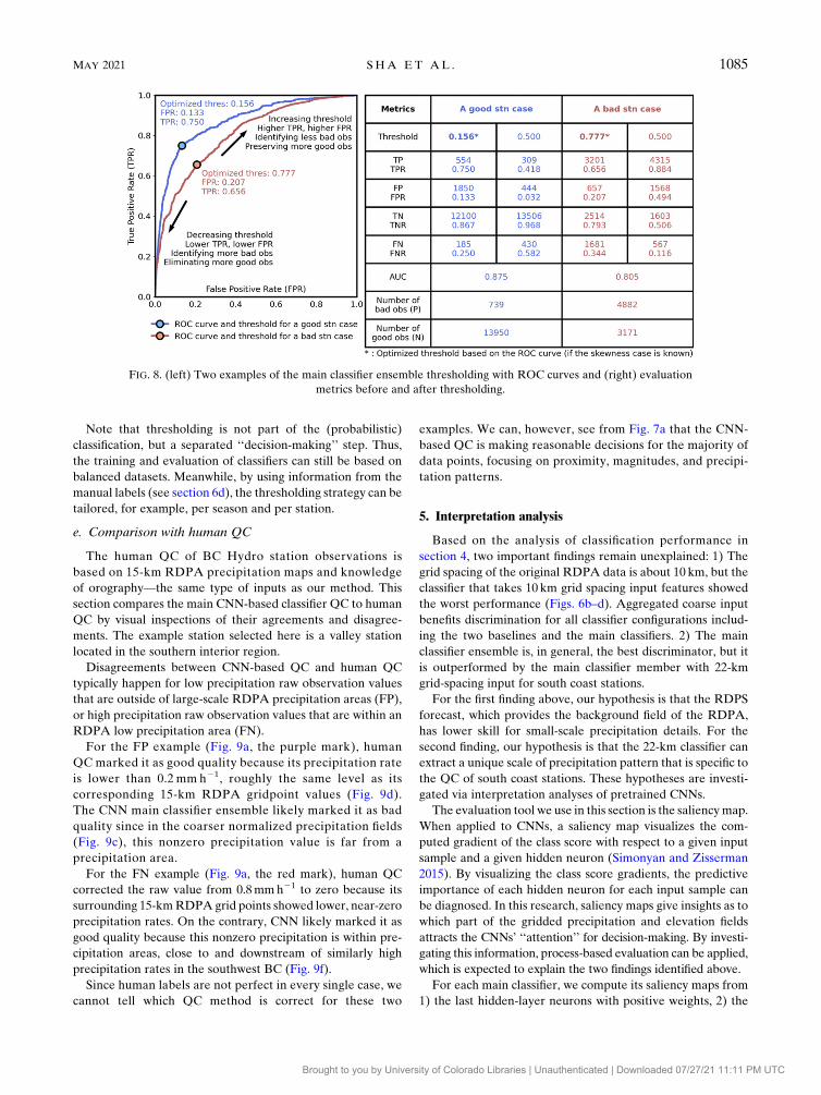
The illustration of classifier thresholding is based on syn-

thesized ‘‘good station’’ and ‘‘bad station’’ cases. Good stations

are positively skewed, with condition positive (P) smaller than

condition negative (N; P � N); whereas the bad stations are

negatively skewed, with N � P. We pick the first and last 25

stations in the rankings of N/P ratio for the above data syn-

thesis. On average, good stations contain 95% good-quality

raw values, whereas for bad stations this ratio is 39% (Fig. 8,

right panel).

When a new station joins the observation network, no prior

can be provided regarding its proportion of good and bad

observations, one may choose 0.5 as the threshold. However, if

this new station does not produce a comparable number of

good and bad observations, the threshold of 0.5 can lead to

suboptimal QC performance. If manual labels became avail-

able after the new station was established, then a thresholding

step could be conducted. Figure 8 provides examples of this

ROC-based thresholding that maximizes the difference of true

positive (TP) and false positive (FP), with a grid search from

0.001 to 0.999. For the good station case, the optimized

threshold is lower than 0.5, which identifies more bad obser-

vations by eliminating slightly more good observations, vice

versa for the ‘‘bad station’’ case.

The QC performance is slightly worse for the bad stations,

with a lower AUC (0.805, compared with 0.875 for the good

stations (Fig. 8). However, given that for all 80 stations in-

volved in this research, the overall percentage of goodQC flags

is 71.7% [see section 3e(1)], new stations are more likely to be

similar to the ‘‘good station’’ case, where theQC classifiers and

relatively low thresholds are expected to perform well.

FIG. 7. Regional evaluation metrics for the main classifiers for (a) south coast stations, (b) southern interior stations, and (c) northeast BC

stations. Text in the top right of each row shows theAUCs of themain classifier ensemble andbest single classifiermember, and the numberof

positive and negative samples that support this evaluation.

TABLE 3. Evaluation metrics for the main classifier ensemble for different seasons in the testing set, and specifically for solid, winter

precipitation. The threshold of the classifier is 0.5.

Seasona TP (TPR) FP (FPR) TN (TNR) FN (FNR) AUC TP 1 FN TN 1 FP

DJF 1512 (0.869) 286 (0.176) 1339 (0.824) 228 (0.131) 0.846 1740 1625

DJF, solid precipitationb 1075 (0.913) 326 (0.319) 695 (0.681) 102 (0.087) 0.797 1177 1021

MAM 1313 (0.848) 249 (0.152) 1389 (0.848) 235 (0.152) 0.848 1548 1638

JJA 1493 (0.853) 252 (0.145) 1484 (0.855) 257 (0.147) 0.854 1750 1736

SON 1421 (0.855) 253 (0.149) 1448 (0.851) 241 (0.145) 0.853 1662 1701

a Part of the February, April, June, and October days are not covered by the testing set (see section 3d).b Solid precipitation is assumed to occur at air temperatures below 21.08C.



Note that thresholding is not part of the (probabilistic)

classification, but a separated ‘‘decision-making’’ step. Thus,

the training and evaluation of classifiers can still be based on

balanced datasets. Meanwhile, by using information from the

manual labels (see section 6d), the thresholding strategy can be

tailored, for example, per season and per station.

e. Comparison with human QC

The human QC of BC Hydro station observations is

based on 15-km RDPA precipitation maps and knowledge

of orography—the same type of inputs as our method. This

section compares the main CNN-based classifier QC to human

QC by visual inspections of their agreements and disagree-

ments. The example station selected here is a valley station

located in the southern interior region.

Disagreements between CNN-based QC and human QC

typically happen for low precipitation raw observation values

that are outside of large-scale RDPA precipitation areas (FP),

or high precipitation raw observation values that are within an

RDPA low precipitation area (FN).

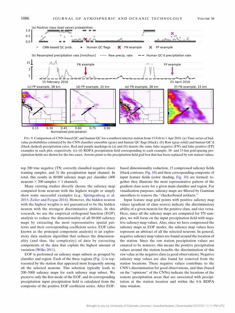
For the FP example (Fig. 9a, the purple mark), human

QC marked it as good quality because its precipitation rate

is lower than 0.2 mm h21, roughly the same level as its

corresponding 15-km RDPA gridpoint values (Fig. 9d).

The CNN main classifier ensemble likely marked it as bad

quality since in the coarser normalized precipitation fields

(Fig. 9c), this nonzero precipitation value is far from a

precipitation area.

For the FN example (Fig. 9a, the red mark), human QC

corrected the raw value from 0.8mmh21 to zero because its

surrounding 15-kmRDPAgrid points showed lower, near-zero

precipitation rates. On the contrary, CNN likely marked it as

good quality because this nonzero precipitation is within pre-

cipitation areas, close to and downstream of similarly high

precipitation rates in the southwest BC (Fig. 9f).

Since human labels are not perfect in every single case, we

cannot tell which QC method is correct for these two

examples. We can, however, see from Fig. 7a that the CNN-

based QC is making reasonable decisions for the majority of

data points, focusing on proximity, magnitudes, and precipi-

tation patterns.

5. Interpretation analysis

Based on the analysis of classification performance in

section 4, two important findings remain unexplained: 1) The

grid spacing of the original RDPA data is about 10 km, but the

classifier that takes 10 km grid spacing input features showed

the worst performance (Figs. 6b–d). Aggregated coarse input

benefits discrimination for all classifier configurations includ-

ing the two baselines and the main classifiers. 2) The main

classifier ensemble is, in general, the best discriminator, but it

is outperformed by the main classifier member with 22-km

grid-spacing input for south coast stations.

For the first finding above, our hypothesis is that the RDPS

forecast, which provides the background field of the RDPA,

has lower skill for small-scale precipitation details. For the

second finding, our hypothesis is that the 22-km classifier can

extract a unique scale of precipitation pattern that is specific to

the QC of south coast stations. These hypotheses are investi-

gated via interpretation analyses of pretrained CNNs.

The evaluation tool we use in this section is the saliencymap.

When applied to CNNs, a saliency map visualizes the com-

puted gradient of the class score with respect to a given input

sample and a given hidden neuron (Simonyan and Zisserman

2015). By visualizing the class score gradients, the predictive

importance of each hidden neuron for each input sample can

be diagnosed. In this research, saliency maps give insights as to

which part of the gridded precipitation and elevation fields

attracts the CNNs’ ‘‘attention’’ for decision-making. By investi-

gating this information, process-based evaluation can be applied,

which is expected to explain the two findings identified above.

For each main classifier, we compute its saliency maps from

1) the last hidden-layer neurons with positive weights, 2) the

FIG. 8. (left) Two examples of the main classifier ensemble thresholding with ROC curves and (right) evaluation

metrics before and after thresholding.



top 200 true negative (TN; correctly classified negative class)

training samples, and 3) the precipitation input channel. In

total, this results in 80 000 saliency maps per classifier (400

neurons 3 200 samples 3 1 channel).

Many existing studies directly choose the saliency map

computed from neurons with the highest weight or simply

show some successful examples (e.g., Springenberg et al.

2015; Zeiler and Fergus 2014). However, the hidden neuron

with the highest weights is not guaranteed to be the hidden

neuron with the strongest discriminative abilities. In this

research, we use the empirical orthogonal function (EOF)

analysis to reduce the dimensionality of all 80 000 saliency

maps by extracting the most representative spatial pat-

terns and their corresponding coefficient series. EOF (also

known as the principal component analysis) is an explor-

atory data analysis algorithm that reduces the dimension-

ality (and thus, the complexity) of data by extracting

components of the data that explain the highest amount of

variation (Wilks 2011).

EOF is performed on saliency maps subsets as grouped by

classifier and region. Each of the three regions (Fig. 1) is rep-

resented by the station that appeared most frequently among

all the selected neurons. This selection typically leads to

200–5000 saliency maps for each saliency map subset. We

preserve only the first mode of the EOF, and its corresponding

precipitation input precipitation field is calculated from the

composite of the positive EOF coefficient series. After EOF-

based dimensionality reduction, 15 compressed saliency fields

(black contours, Fig. 10) and their corresponding composite of

input feature fields (color shading, Fig. 10) are formed; to-

gether they illustrate the most representative pattern of the

gradient class score for a given main classifier and region. For

visualization purposes, saliency maps are filtered by Gaussian

smoothers to remove the ‘‘checkerboard artifacts.’’

Input feature map grid points with positive saliency map

values (gradient of class scores) indicate the discriminatory

ability of a given neuron for the positive class, and vice versa.

Here, since all the saliency maps are computed for TN sam-

ples, we will focus on the input precipitation field with nega-

tive saliency map values. Also, since we have compressed the

saliency maps as EOF modes, the saliency map values here

represent an abstract of all the selected neurons. In general,

negative saliency map values are found around the location of

the station. Since the raw station precipitation values are

ensured to be nonzero, this means the positive precipitation

values around the station benefits the discrimination of this

raw value as the negative class (a good observation). Negative

saliency map values are also found far removed from the

station locations. These negative values contribute to the

CNN’s discrimination for good observations, and thus (based

on the ‘‘opinions’’ of the CNNs) indicate the locations of the

remote precipitation areas that are associated with precipi-

tation at the station location and within the 6-h RDPA

time window.

FIG. 9. Comparison of CNN-basedQC and humanQC for a southern interior station from 15 Feb to 1 Apr 2016. (a) Time series of bad-

value probabilities estimated by the CNN classifier ensemble (gray) and human QC flags (black). (b) Raw (gray solid) and human-QC’d

(black dashed) precipitation rates. Red and purple markings in (a) and (b) denote the same false negative (FN) and false positive (FP)

examples in each plot, respectively. (c)–(f) RDPA precipitation field corresponding to each example; 38- and 15-km grid-spacing pre-

cipitation fields are shown for the two cases. Arrows point to the precipitation field grid box that has been replaced by raw station values.



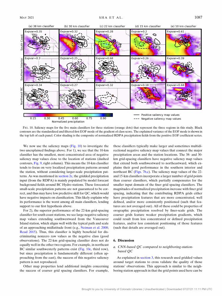
We now use the saliency maps (Fig. 10) to investigate the

two unexplained findings above. For 1), we see that the 10-km

classifier has the smallest, most concentrated area of negative

saliency map values close to the location of stations (dashed

contours, Fig. 9, right column). This means the 10-km classifier

tends to focus on very localized precipitation patterns around

the station, without considering larger-scale precipitation pat-

terns. As was mentioned in section 2c, the gridded precipitation

input (from the RDPA) is mainly populated by model forecast

background fields around BC Hydro stations. These forecasted

small-scale precipitation patterns are not guaranteed to be cor-

rect, and thus may have low predictive skill for QC, whichwould

have negative impacts on classification. This likely explains why

its performance is the worst among all main classifiers, lending

support to our first hypothesis above.

For 2), the superior performance of the 22-km grid-spacing

classifier for south coast stations, we see large negative saliency

map values extending southwestward from the Vancouver

Island station, which aligns well with the typical path and scale

of an approaching midlatitude front (e.g., Neiman et al. 2008;

Read 2015). Thus, this classifier is highly beneficial for dis-

criminating nonzero raw values as the negative class (good

observations). The 22-km grid-spacing classifier does not do

equally well in the other two regions. For example, in northeast

BC similar southwesterly patterns exist (Fig. 10c, third row),

but since precipitation is fundamentally different (often ap-

proaching from the east), the success of this negative saliency

pattern is not reproduced.

Other map properties lend additional insights concerning

the success of coarser grid spacing classifiers. For example,

these classifiers typically make larger and sometimes multidi-

rectional negative saliency map values that connect the major

precipitation areas and the station locations. The 38- and 30-

km grid-spacing classifiers have negative saliency map values

that extend both southwestward to northeastward, which ex-

plains their good performance in the southern interior and

northeast BC (Figs. 7b,c). The saliency map values of the 22-

and 15-km classifiers incorporate a larger number of grid points

than coarser classifiers, which partially compensates for the

smaller input domain of the finer grid spacing classifiers. The

magnitudes of normalized precipitation increase with finer grid

spacing, indicating that the contributing RDPA grids either

have precipitation features that are more concentrated, well

defined, and/or more consistently positioned (such that fea-

tures are not averaged out). All of these could be properties of

orographic precipitation resolved by finer-scale grids. The

coarser grids feature weaker precipitation gradients, which

could result from less concentrated or defined precipitation

features, and/or less consistent positioning of those features

(such that details are averaged out).

6. Discussion

a. CNN-based QC compared to neighboring-station-based QC

As explained in section 3, this research used gridded values

around target stations to cross validate the quality of those

stations’ observations. This approach is similar to the neigh-

boring station approach in that the grid points used here can be

FIG. 10. Saliency maps for the five main classifiers for three stations (orange dots) that represent the three regions in this study. Black

contours are the standardized and filtered first EOFmode of the gradient of class score. The explained variance of the EOFmode is shown in

the top left of each panel. Color shading is the composite of normalized RDPA precipitation fields from the positive EOF coefficient series.



viewed as the ‘‘surrogate stations.’’ Individual RDPA grid

point values are not as reliable as good-quality station obser-

vations; however, collectively the 64 3 64 sized inputs provide

useful information for cross validating the target station

observations.

Compared to the classic neighboring station approach (e.g.,

Hubbard et al. 2005), the use of gridded data has advantages

for QC’ing stations in complex terrain regions and/or regions

where reference stations are sparse.We have shown that CNN-

based classifiers can effectively use spatial patterns from both

precipitation and elevation gridded inputs for station obser-

vationQC, and the classification result is largely improved over

spatially agnostic models like MLP and decision trees. We

think this finding further implies the potential of deep-

learning-based QC as an alternative to other automated QC

methods for handling more diverse input data forms.

b. Notes on data skewness

Our method was trained on a balanced dataset and based on

the evaluations in section 4c, it performs well for positively

skewed (more good observations than bad observations) sta-

tions. This guarantees the reliability of our method for most

BC Hydro stations. For the uncommon ‘‘bad stations,’’ where

QC flags are negatively skewed, some solutions are available.

For example, prior stand-alone checks, such as range checks,

common bad value checks and rate of change checks can re-

duce the number of positive samples. Additionally, one could

create a small human-QC’d validation dataset for the nega-

tively skewed station, and tune QC classifiers on that dataset

(e.g., Platt 1999; Niculescu-Mizil and Caruana 2005). This fine-

tuning can be performed at either the ensemble level or the

single classifier level.

Another problem typically associated with data skewness is

the ‘‘precision-recall tradeoff’’—the trade-off between maxi-

mizing TPR and TNR. As shown in Figs. 5 and 6, the main

classifier ensemble is a balanced classifier—for a balanced

testing set, it classifies good and bad observations equally well.

In an operational setting with big data pools, higher TNR

(lower type II error) could be more important. That is, users

may prefer to lose (misclassify) some good observations to

correctly eliminate more bad observations (minimize FNR),

due to the larger downstream impacts of bad observations.

This is an important point: a user can choose to improve the

system’s FNR by simply lowering the threshold of bad-

observation probability (i.e., below 0.5).

c. Generalization and input data replacement

Our method requires gridded precipitation data as an input,

and in this research, the RDPA is applied. Could one use other

gridded precipitation data to replace the RDPA for other ob-

servation networks and outside of BC?

Based on the interpretation analysis in section 5, our method

implicitly compares a gauge observational value with its sur-

rounding precipitation patterns from a gridded analysis. Many

successfully QC’d nonzero gauge observations are located ei-

ther within or at the edge of a synoptic-scale precipitation

pattern. This finding is identified for 38–15-km grid-spacing

inputs and both coastal and interior watersheds—it is not

specific to a certain grid spacing or geographical location. That

said, if a gridded input other than the RDPA can roughly

represent the spatial coverage of precipitation events, then we

have no a priori reason to expect the performance would be

downgraded. We think exploiting different gridded inputs as

QC reference fields is a possible future research direction.

Further, as described in section 3a, the CNN-based QC is

based on pattern-to-station rather than gridpoint-to-station

comparisons, and thus, it has some robustness against the po-

sition errors of gridded precipitation data. For most of the BC

Hydro watersheds in this research, the RDPA is mainly pop-

ulated by the RDPS forecast model, with limited precipitation

gauge calibrations. This deficiency impacted the CNN-base

methods less than the other two external baselines. Thus, for

generalizing CNN-based observation QC to a broader extent,

one could either adapt the classifier configuration and data

preprocessing of this research, or build new CNN classifiers

from scratch. However, we do recommend a post hoc inter-

pretation analysis, similar to our section 5, to ensure that the

proposed CNNs are utilizing precipitation pattern information.

d. Learning from and collaborative improvement of

the CNNs

Machine learning interpretation methods like the saliency

maps employed herein give insights into the decision-making

of the CNN-based QCmodel. These insights can, in turn, bring

inspiration to human QC procedures. Based on the compari-

sons in section 4d and interpretations in section 5, the CNN

values the distribution of precipitation patterns upstream of

the station. This suggests that human QC should also focus

more on cross validations using stations/data sources upstream

of a target station, rather than simply looking at all nearby

values. Based on the intercomparison of main classifier mem-

bers, regridding precipitation data to coarser grid spacings may

be another way to improve manual and/or automated QC

workflows.

Human QC staff could also work collaboratively with the

CNN-based QC. One possible configuration would be for the

CNNs to perform the first round of QC to categorize high-

confidence good and bad observations. The human QC staff

would then perform a second round to categorize the obser-

vations that have less certain quality probabilities close to 0.5.

The above combination reduces human workload and gives

them more time to focus on the more important and difficult

QC cases. Also, when the second round human QC is com-

pleted, the resulting QC labels can be used to further tune and

improve the classification performance and thresholding of

the CNN.

7. Conclusions

We proposed ResNet-like CNNs with multiscale classifier

ensembles for the automated QC of a sparse precipitation

observation network in complex terrain. The CNNs are

trained with human QC’d labels through supervised learn-

ing and can classify raw observation values by taking re-

gridded (coarsened) precipitation analyses (RDPA) and elevation

(ETOPO1) as inputs. Based on classification metrics, our



CNN-based QC separates ‘‘good’’ and ‘‘bad’’ observations

well, with an overall area under curve (AUC) of 0.927 and type

I/type II error lower than 15%.

Our approach has minor limitations when handling 1) solid

precipitation in DJF and 2) very problematic stations (stations

where bad observations largely outnumber the good). Solid

precipitation QC tends to eliminate somewhat more good

observations, but the preserved values are still of good quality.

The issue with problematic stations could be overcome by fine-

tuning the model for these types of stations using a smaller

human-labeled dataset. Aside from these limitations, our

CNN-based QC is effective and could be generalized to other

observation networks for a variety of use cases.

To our knowledge, this is the first study that implements

CNN classifiers for precipitation observation quality control,

and explains why CNNs can make better QC decisions. We

found that coarser grid spacing (i.e., 38-, 30-, 22-km) inputs

yielded better CNN performance, and the CNNs can detect

abnormal nonzero raw observational values by taking into

account the station locations relative to other neighboring

and upstream precipitation patterns. This saliency infor-

mation learned from CNNs could also help inform human

QC operations.

Acknowledgments. This research is jointly funded by a Four

Year Doctoral Fellowship (4YF) program of the University

of British Columbia, and the Canadian Natural Science and

Engineering Research Council (NSERC). We thank BC

Hydro, and the Environment and Climate Change Canada

(ECCC) for providing the data.Wealso thank theCasper cluster

[Computational and Information Systems Laboratory (CISL);

CISL 2020], the National Center for Atmospheric Research

(NCAR), and their Advanced Study Program (ASP) for sup-

porting this research. NCAR is operated by the University

Corporation for Atmospheric Research (UCAR) and is spon-

sored by the National Science Foundation. Additional support

was provided by MITACS and BC Hydro. We also thank the

three anonymous reviewers for their comments and suggestions

which improved this manuscript.

REFERENCES

Adam, J. C., and D. P. Lettenmaier, 2003: Adjustment of global

gridded precipitation for systematic bias: Global gridded

precipitation. J. Geophys. Res., 108, 4257, https://doi.org/

10.1029/2002JD002499.

Adler, R. F., and Coauthors, 2003: The version-2 Global Precipitation

Climatology Project (GPCP) monthly precipitation analysis

(1979–present). J. Hydrometeor., 4, 1147–1167, https://doi.org/

10.1175/1525-7541(2003)004,1147:TVGPCP.2.0.CO;2.

Amante, C., and B. Eakins, 2009: ETOPO1 Arc-Minute Global

Relief Model: Procedures, data sources and analysis. National

Geophysical Data Center Marine Geology and Geophysics

Division Rep., 25 pp.

Banta, R. M., and Coauthors, 2013: Observational techniques:

Sampling the mountain atmosphere. Mountain Weather

Research and Forecasting: Recent Progress and Current

Challenges, F. K. Chow, S. F. De Wekker, and B. J. Snyder,

Eds., Springer Atmospheric Sciences, 409–530, https://

doi.org/10.1007/978-94-007-4098-3_8.

BC Hydro, 2020: Generation System: An efficient, low cost

electricity system for B.C. Accessed 13 May 2020, https://

www.bchydro.com/energy-in-bc/operations/generation.html.

Breiman, L., 1996: Bagging predictors. Mach. Learn., 24, 123–140,

https://doi.org/10.1007/BF00058655.

——, J. H. Friedman, R. A. Olshen, and C. J. Stone, 2017:

Classification and Regression Trees. 1st ed. Routledge, 368 pp.,

https://doi.org/10.1201/9781315139470.

Canadian Centre for Climate Services, 2019: Technical documenta-

tion: Regional Deterministic Precipitation Analysis (RDPA).

Government of Canada, https://www.canada.ca/en/environment-

climate-change/services/climate-change/canadian-centre-

climate-services/display-download/technical-documentation-

regional-precipitation-analysis.html.

Carrera, M. L., S. Bélair, V. Fortin, B. Bilodeau, D. Charpentier,

and I. Doré, 2010: Evaluation of snowpack simulations over

the Canadian Rockies with an experimental hydrometeoro-

logical modeling system. J. Hydrometeor., 11, 1123–1140,

https://doi.org/10.1175/2010JHM1274.1.

Chilton, R. R. H., 1981: A summary of climatic regimes of British

Columbia.Ministry of Environment Assessment and Planning

Division Rep., 44 pp.

CISL, 2020: Cheyenne: HPE/SGI ICEXA system (NCARCommunity

Computing). National Center for Atmospheric Research, https://

doi.org/10.5065/d6rx99hx.

Eischeid, J. K., C. B. Baker, T. R. Karl, and H. F. Diaz, 1995: The

quality control of long-term climatological data using objective

data analysis. J. Appl. Meteor., 34, 2787–2795, https://doi.org/

10.1175/1520-0450(1995)034,2787:TQCOLT.2.0.CO;2.

——, P. A. Pasteris, H. F. Diaz, M. S. Plantico, and N. J. Lott, 2000:

Creating a serially complete, national daily time series of

temperature and precipitation for the western United States.

J. Appl. Meteor., 39, 1580–1591, https://doi.org/10.1175/1520-

0450(2000)039,1580:CASCND.2.0.CO;2.

Fortin, V., G. Roy, N. Donaldson, and A. Mahidjiba, 2015:

Assimilation of radar quantitative precipitation estimations in

the Canadian Precipitation Analysis (CaPA). J. Hydrol., 531,

296–307, https://doi.org/10.1016/j.jhydrol.2015.08.003.

——,——, T. Stadnyk, K. Koenig, N. Gasset, and A. Mahidjiba, 2018:

Ten years of science based on theCanadianPrecipitationAnalysis:

A CaPA system overview and literature review. Atmos.–Ocean,

56, 178–196, https://doi.org/10.1080/07055900.2018.1474728.Goodfellow, I., Y. Bengio, and A. Courville, 2016:Deep Learning:

Adaptive Computation and Machine Learning. MIT Press,

775 pp.

Goodison, B. E., P. Y. T. Louie, and D. Yang, 1998: WMO solid pre-

cipitation measurement intercomparison—Final report. WMO

Rep. 67, 318 pp., https://www.wmo.int/pages/prog/www/IMOP/

publications/IOM-67-solid-precip/WMOtd872.pdf.

Groisman, P. Ya., and D. R. Legates, 1994: The accuracy of

United States precipitation data. Bull. Amer. Meteor.

Soc., 75, 215–228, https://doi.org/10.1175/1520-0477(1994)

075,0215:TAOUSP.2.0.CO;2.

Gu, J., and Coauthors, 2018: Recent advances in convolutional

neural networks. Pattern Recognit., 77, 354–377, https://doi.org/

10.1016/j.patcog.2017.10.013.

He, K., X. Zhang, S. Ren, and J. Sun, 2015a: Deep residual learning

for image recognition. arXiv, http://arxiv.org/abs/1512.03385.

——, ——, ——, and ——, 2015b: Delving deep into rectifiers:

surpassing human-level performance on ImageNet clas-

sification. 2015 IEEE Int. Conf. on Computer Vision,

IEEE, Santiago, Chile, 1026–1034, https://doi.org/10.1109/

ICCV.2015.123.



https://doi.org/10.1029/2002JD002499

https://doi.org/10.1029/2002JD002499

https://doi.org/10.1175/1525-7541(2003)004<1147:TVGPCP>2.0.CO;2

https://doi.org/10.1175/1525-7541(2003)004<1147:TVGPCP>2.0.CO;2

https://doi.org/10.1007/978-94-007-4098-3_8

https://doi.org/10.1007/978-94-007-4098-3_8

https://www.bchydro.com/energy-in-bc/operations/generation.html

https://www.bchydro.com/energy-in-bc/operations/generation.html

https://doi.org/10.1007/BF00058655

https://doi.org/10.1201/9781315139470

https://www.canada.ca/en/environment-climate-change/services/climate-change/canadian-centre-climate-services/display-download/technical-documentation-regional-precipitation-analysis.html




https://doi.org/10.1175/2010JHM1274.1

https://doi.org/10.5065/d6rx99hx

https://doi.org/10.5065/d6rx99hx

https://doi.org/10.1175/1520-0450(1995)034<2787:TQCOLT>2.0.CO;2

https://doi.org/10.1175/1520-0450(1995)034<2787:TQCOLT>2.0.CO;2

https://doi.org/10.1175/1520-0450(2000)039<1580:CASCND>2.0.CO;2

https://doi.org/10.1175/1520-0450(2000)039<1580:CASCND>2.0.CO;2

https://doi.org/10.1016/j.jhydrol.2015.08.003

https://doi.org/10.1080/07055900.2018.1474728

https://www.wmo.int/pages/prog/www/IMOP/publications/IOM-67-solid-precip/WMOtd872.pdf

https://www.wmo.int/pages/prog/www/IMOP/publications/IOM-67-solid-precip/WMOtd872.pdf

https://doi.org/10.1175/1520-0477(1994)075<0215:TAOUSP>2.0.CO;2

https://doi.org/10.1175/1520-0477(1994)075<0215:TAOUSP>2.0.CO;2

https://doi.org/10.1016/j.patcog.2017.10.013

https://doi.org/10.1016/j.patcog.2017.10.013

http://arxiv.org/abs/1512.03385

https://doi.org/10.1109/ICCV.2015.123

https://doi.org/10.1109/ICCV.2015.123

Hubbard, K. G., S. Goddard, W. D. Sorensen, N. Wells, and T. T.

Osugi, 2005: Performance of quality assurance procedures for

an applied climate information system. J. Atmos. Oceanic

Technol., 22, 105–112, https://doi.org/10.1175/JTECH-1657.1.

Ioffe, S., and C. Szegedy, 2015: Batch normalization: Accelerating

deep network training by reducing internal covariate shift.

arXiv, http://arxiv.org/abs/1502.03167.

Jiang, S., M. Lian, C. Lu, Q. Gu, S. Ruan, and X. Xie, 2018:

Ensemble prediction algorithm of anomaly monitoring

based on big data analysis platform of open-pit mine slope.

Complexity, 2018, 1048756, https://doi.org/10.1155/2018/

1048756.

Jørgensen, H. K., S. Rosenørn, H. Madsen, and P. S. Mikkelsen,

1998: Quality control of rain data used for urban runoff sys-

tems.Water Sci. Technol., 37, 113–120, https://doi.org/10.2166/

wst.1998.0448.

Kienzle, S. W., 2008: A new temperature based method to separate

rain and snow. Hydrol. Processes, 22, 5067–5085, https://

doi.org/10.1002/hyp.7131.

Kingma, D. P., and J. Ba, 2017: Adam: A method for stochastic

optimization. arXiv, http://arxiv.org/abs/1412.6980.

Lakshmanan, V., A. Fritz, T. Smith, K. Hondl, and G. Stumpf,

2007: An automated technique to quality control radar re-

flectivity data. J. Appl. Meteor. Climatol., 46, 288–305, https://

doi.org/10.1175/JAM2460.1.

——, C. Karstens, J. Krause, and L. Tang, 2014: Quality control of

weather radar data using polarimetric variables. J. Atmos.

Oceanic Technol., 31, 1234–1249, https://doi.org/10.1175/JTECH-

D-13-00073.1.

Lespinas, F., V. Fortin, G. Roy, P. Rasmussen, and T. Stadnyk,

2015: Performance evaluation of the Canadian Precipitation

Analysis (CaPA). J. Hydrometeor., 16, 2045–2064, https://

doi.org/10.1175/JHM-D-14-0191.1.

Liu, Y., and Coauthors, 2016: Application of deep convolutional

neural networks for detecting extreme weather in climate

datasets. arXiv, http://arxiv.org/abs/1605.01156.

——, G. Ren, X. Sun, and X. Li, 2018: A new method to separate

precipitation phases. Hydrol. Earth Syst. Sci. Discuss., https://

doi.org/10.5194/hess-2018-307.

Mahfouf, J.-F., B. Brasnett, and S. Gagnon, 2007: A Canadian

Precipitation Analysis (CaPA) project: Description and pre-

liminary results. Atmos.–Ocean, 45, 1–17, https://doi.org/

10.3137/ao.v450101.

Martinaitis, S. M., S. B. Cocks, Y. Qi, B. T. Kaney, J. Zhang, and

K. Howard, 2015: Understanding winter precipitation impacts

on automated gauge observations within a real-time system.

J. Hydrometeor., 16, 2345–2363, https://doi.org/10.1175/JHM-

D-15-0020.1.

Maul-Kötter, B., and T. Einfalt, 1998: Correction and preparation

of continuously measured raingauge data: A standard method

in North Rhine-Westphalia. Water Sci. Technol., 37, 155–162,

https://doi.org/10.2166/wst.1998.0458.

Meek, D., and J. Hatfield, 1994: Data quality checking for single

station meteorological databases. Agric. For. Meteor., 69,

85–109, https://doi.org/10.1016/0168-1923(94)90083-3.

Motoyama, H., 1990: Simulation of seasonal snowcover based

on air temperature and precipitation. J. Appl. Meteor., 29,

1104–1110, https://doi.org/10.1175/1520-0450(1990)029,1104:

SOSSBO.2.0.CO;2.

Mourad, M., and J.-L. Bertrand-Krajewski, 2002: A method for

automatic validation of long time series of data in urban hy-

drology. Water Sci. Technol., 45, 263–270, https://doi.org/

10.2166/wst.2002.0601.

Nearing, M. A., and Coauthors, 2005: Modeling response of soil

erosion and runoff to changes in precipitation and cover.Catena,

61, 131–154, https://doi.org/10.1016/j.catena.2005.03.007.

Neiman, P. J., F. M. Ralph, G. A. Wick, J. D. Lundquist, andM. D.

Dettinger, 2008: Meteorological characteristics and overland

precipitation impacts of atmospheric rivers affecting the west

coast of North America based on eight years of SSM/I satellite

observations. J. Hydrometeor., 9, 22–47, https://doi.org/10.1175/

2007JHM855.1.

Niculescu-Mizil, A., and R. Caruana, 2005: Predicting good prob-

abilities with supervised learning. Proc. 22nd Int. Conf. on

Machine Learning, Bonn, Germany, ACM, 625–632, https://

doi.org/10.1145/1102351.1102430.

Null, S. E., J. H. Viers, and J. F. Mount, 2010: Hydrologic response

and watershed sensitivity to climate warming in California’s

Sierra Nevada. PLOS ONE, 5, e9932, https://doi.org/10.1371/

journal.pone.0009932.

Odon, P., G. West, and R. Stull, 2018: Evaluation of reanalyses

over British Columbia. Part I: Daily and extreme 2-m tem-

perature. J. Appl. Meteor. Climatol., 57, 2091–2112, https://

doi.org/10.1175/JAMC-D-18-0058.1.

Piatyszek, E., P. Voignier, and D. Graillot, 2000: Fault detection

on a sewer network by a combination of a Kalman filter and a

binary sequential probability ratio test. J. Hydrol., 230, 258–

268, https://doi.org/10.1016/S0022-1694(00)00213-4.

Platt, J. C., 1999: Probabilistic outputs for support vector machines

and comparisons to regularized likelihoodmethods.Advances

in Large Margin Classifiers, MIT Press, 61–74.

Qi, Y., S. Martinaitis, J. Zhang, and S. Cocks, 2016: A real-time

automated quality control of hourly rain gauge data based

on multiple sensors in MRMS system. J. Hydrometeor., 17,

1675–1691, https://doi.org/10.1175/JHM-D-15-0188.1.

Raileanu, L. E., and K. Stoffel, 2004: Theoretical comparison

between the Gini index and information gain criteria. Ann.

Math. Artif. Intell., 41, 77–93, https://doi.org/10.1023/B:

AMAI.0000018580.96245.c6.

Rasmussen, R., and Coauthors, 2012: How well are we measuring

snow: The NOAA/FAA/NCAR winter precipitation test bed.

Bull. Amer. Meteor. Soc., 93, 811–829, https://doi.org/10.1175/

BAMS-D-11-00052.1.

Read, W. A., 2015: The climatology and meteorology of wind-

storms that affect southwest British Columbia, Canada, and

associated tree-related damage to the power distribution grid.

Ph.D. thesis, University of British Columbia, 383 pp., https://

doi.org/10.14288/1.0166485.

Schneider, U., A. Becker, P. Finger, A.Meyer-Christoffer, M. Ziese,

and B. Rudolf, 2014: GPCC’s new land surface precipitation

climatology based on quality-controlled in situ data and its role

in quantifying the global water cycle. Theor. Appl. Climatol.,

115, 15–40, https://doi.org/10.1007/s00704-013-0860-x.Sciuto, G., B. Bonaccorso, A. Cancelliere, and G. Rossi, 2009:

Quality control of daily rainfall data with neural net-

works. J. Hydrol., 364, 13–22, https://doi.org/10.1016/

j.jhydrol.2008.10.008.

Simonyan, K., and A. Zisserman, 2015: Very deep convolutional

networks for large-scale image recognition. arXiv, http://

arxiv.org/abs/1409.1556.

Springenberg, J. T., A. Dosovitskiy, T. Brox, and M. Riedmiller,

2015: Striving for simplicity: The all convolutional net. arXiv,

http://arxiv.org/abs/1412.6806.�St�epánek, P., P. Zahradnícek, and P. Skalák, 2009: Data quality

control and homogenization of air temperature and precipi-

tation series in the area of the Czech Republic in the period



https://doi.org/10.1175/JTECH-1657.1


https://doi.org/10.1155/2018/1048756

https://doi.org/10.1155/2018/1048756

https://doi.org/10.2166/wst.1998.0448

https://doi.org/10.2166/wst.1998.0448

https://doi.org/10.1002/hyp.7131

https://doi.org/10.1002/hyp.7131


https://doi.org/10.1175/JAM2460.1

https://doi.org/10.1175/JAM2460.1

https://doi.org/10.1175/JTECH-D-13-00073.1

https://doi.org/10.1175/JTECH-D-13-00073.1

https://doi.org/10.1175/JHM-D-14-0191.1



https://doi.org/10.5194/hess-2018-307

https://doi.org/10.5194/hess-2018-307

https://doi.org/10.3137/ao.v450101

https://doi.org/10.3137/ao.v450101



https://doi.org/10.2166/wst.1998.0458

https://doi.org/10.1016/0168-1923(94)90083-3

https://doi.org/10.1175/1520-0450(1990)029<1104:SOSSBO>2.0.CO;2

https://doi.org/10.1175/1520-0450(1990)029<1104:SOSSBO>2.0.CO;2

https://doi.org/10.2166/wst.2002.0601

https://doi.org/10.2166/wst.2002.0601

https://doi.org/10.1016/j.catena.2005.03.007

https://doi.org/10.1175/2007JHM855.1

https://doi.org/10.1175/2007JHM855.1

https://doi.org/10.1145/1102351.1102430

https://doi.org/10.1145/1102351.1102430

https://doi.org/10.1371/journal.pone.0009932

https://doi.org/10.1371/journal.pone.0009932

https://doi.org/10.1175/JAMC-D-18-0058.1


https://doi.org/10.1016/S0022-1694(00)00213-4


https://doi.org/10.1023/B:AMAI.0000018580.96245.c6

https://doi.org/10.1023/B:AMAI.0000018580.96245.c6

https://doi.org/10.1175/BAMS-D-11-00052.1

https://doi.org/10.1175/BAMS-D-11-00052.1

https://doi.org/10.14288/1.0166485

https://doi.org/10.14288/1.0166485

https://doi.org/10.1007/s00704-013-0860-x






1961–2007.Adv. Sci. Res., 3, 23–26, https://doi.org/10.5194/asr-

3-23-2009.

Tompson, J., R. Goroshin, A. Jain, Y. LeCun, and C. Bregler,

2015: Efficient object localization using convolutional

networks. 2015 IEEE Conf. on Computer Vision and

Pattern Recognition, Boston, MA, IEEE, 648–656, https://

doi.org/10.1109/CVPR.2015.7298664.

Vandal, T., E. Kodra, S. Ganguly, A. Michaelis, R. Nemani, and A. R.

Ganguly, 2018: Generating high resolution climate change projec-

tions through single image super-resolution: an abridged version.

Proc. 27th Int. Joint Conf. on Artificial Intelligence, Stockholm,

Sweden, International Joint Conferences on Artificial Intelligence

Organization, 5389–5393, https://doi.org/10.24963/ijcai.2018/759.

Wilks, D. S., 2011: Statistical Methods in the Atmospheric Sciences.

3rd ed. Elsevier, 676 pp.

Wong, J. S., S. Razavi, B. R. Bonsal, H. S. Wheater, and Z. E.

Asong, 2017: Inter-comparison of daily precipitation

products for large-scale hydro-climatic applications over

Canada. Hydrol. Earth Syst. Sci., 21, 2163–2185, https://doi.org/10.5194/hess-21-2163-2017.

Xie, P., and P. A. Arkin, 1996: Analyses of global monthly precipita-

tion using gauge observations, satellite estimates, and numerical

model predictions. J. Climate, 9, 840–858, https://doi.org/10.1175/

1520-0442(1996)009,0840:AOGMPU.2.0.CO;2.

Xu, C.-D., J.-F. Wang,M.-G. Hu, andQ.-X. Li, 2014: Estimation of

uncertainty in temperature observations made at meteoro-

logical stations using a probabilistic spatiotemporal approach.

J. Appl. Meteor. Climatol., 53, 1538–1546, https://doi.org/

10.1175/JAMC-D-13-0179.1.

Yang, D., D. Kane, Z. Zhang, D. Legates, and B. Goodison, 2005:

Bias corrections of long-term (1973–2004) daily precipitation

data over the northern regions. Geophys. Res. Lett., 32,

L19501, https://doi.org/10.1029/2005GL024057.

You, J., K. G. Hubbard, S. Nadarajah, and K. E. Kunkel, 2007:

Performance of quality assurance procedures on daily pre-

cipitation. J. Atmos. Oceanic Technol., 24, 821–834, https://

doi.org/10.1175/JTECH2002.1.

Zeiler, M. D., and R. Fergus, 2014: Visualizing and understanding

convolutional networks. 13th European Conf. on Computer

Vision, Zurich, Switzerland, ECCV, https://doi.org/10.1007/

978-3-319-10590-1_53.

Zhao, Q., Y. Zhu, D. Wan, Y. Yu, and X. Cheng, 2018: Research on

the data-driven quality control method of hydrological time

series data. Water, 10, 1712, https://doi.org/10.3390/w10121712.



https://doi.org/10.5194/asr-3-23-2009

https://doi.org/10.5194/asr-3-23-2009

https://doi.org/10.1109/CVPR.2015.7298664

https://doi.org/10.1109/CVPR.2015.7298664

https://doi.org/10.24963/ijcai.2018/759

https://doi.org/10.5194/hess-21-2163-2017

https://doi.org/10.5194/hess-21-2163-2017

https://doi.org/10.1175/1520-0442(1996)009<0840:AOGMPU>2.0.CO;2

https://doi.org/10.1175/1520-0442(1996)009<0840:AOGMPU>2.0.CO;2



https://doi.org/10.1029/2005GL024057

https://doi.org/10.1175/JTECH2002.1

https://doi.org/10.1175/JTECH2002.1

https://doi.org/10.1007/978-3-319-10590-1_53

https://doi.org/10.1007/978-3-319-10590-1_53

https://doi.org/10.3390/w10121712

Documents

Deep-Learning-Based Precipitation Observation Quality Control