Deep electromagnetic sounding in Turkmenia - Geophysical Journal

Geophys. J . Int. (1994) 118, 467-484

Deep electromagnetic sounding in Turkmenia

D. B. Avdeev,' V. G. Dubrovsky,2 E. B. Fainberg,' 0. V. Pankratov' and B. Sh. Zinger' ' Institute of Physics of rhe Earth, Russian Academy of Sciences, 142092, Troitsk, Moscow Region, Russia * Institute of Seismology, Academy of Sciences of Turkmenia, Ashgabat. Turkmenia

Accepted 1993 December 13. Received 1993 December 8; in original form 1993 April 30

SUMMARY This paper presents the results of interpretation of magnetotelluric and magnetovariational observations in a vast region, including the southern part of the Turanian plate and the South Caspian megadepression. Both l-D and 2-D interpretations fail to explain the main peculiarities of the natural magnetotelluric and magnetovariational fields observed in the region. The 3-D interpretation used in the paper is based on thin-sheet modelling and inversion algorithms developed by the authors. The final model consists of an inhomogeneous surface layer and a conductive layer, embedded in the otherwise laterally uniform medium in the crust under the Kopet-Dagh mountains. The surface layer conductance varies between 100 S and 13 OOO S, and the crustal anomaly has a conductance of about 2500 S. The layered regional structure includes a conductive layer at a depth of 80-100 km, whose conductance is about 1800 S. The model explains all of the main features of the observed magnetotelluric and magnetovariational fields in the region.

Key words: asthenospheric layer, crust conductor, 3-D interpretation, inversion, thin-sheet modelling.

1 INTRODUCTION

The region under consideration includes the southern part of the Turanian plate, the geosyncline system of Kopet-Dagh and the South Caspian megadepression (Fig. 1). Since 1962 electromagnetic measurements have been carried out by the Institute of Seismology of the Turkmenian Academy of Sciences. These measurements reveal the complicated structure of electromagnetic fields in the region. A number of papers have been devoted to interpretation of the observations (Avagimov et al. 1978, 1981; Singer et al. 1984). The need to return repeatedly to the data interpretation was mainly connected with two factors. First, new data were acquired as observations continued. Some old observations were corrected with new and more reliable measurements and processing. Second, each stage of interpretation was based on the algorithms and programs available at that moment.

It became quite clear long ago that l-D and 2-D interpretations were insufficient, while full-scale 3-D interpretation was not available. It is still not available. The usual constraint on design of a numerical mesh is that the spacing of adjacent nodes should be less than the effective skin depth. On the other hand the whole mesh size should be greater than the 'adjustment distance', to guarantee that

anomalous fields are negligible at the model's borders. For a number of regions these demands can be satisfied only if the surficial mesh includes as many as lo4 nodes, or more. This is the reason why since 1984 thin-sheet modelling and inversion algorithms have become the main mathematical tools for interpretation of electromagnetic observations in South Turkmenia.

2 BRIEF DESCRIPTION OF THE REGION

From geological and geophysical points of view the region can be roughly classified as the southern slope of the Turanian plate and the South Caspian megadepression (Fig. 1). The southern part of the plate is bordered by a geosyncline zone of alpine folding: the Kopet-Dagh mountains. The geosyncline zone is separated from the plate by the Northern Balkhan and pre-Kopet-Dagh foredeep to the north. To the south it is separated from the Elburs mountains by the South Caspian megadepression and the Kuchan-Mashkhad deep fault. The pre-Kopet-Dagh foredeep is a vast depression 600km ~ 6 0 k m . Ashgabat depression is the deepest part of the foredeep where the depth to the Palaeozoic basement reaches 18-19 km. The southern slope of the plate includes its outskirt strip of 50-70km width. Here the thickness of the sedimentary

467

Dow

nloaded from https://academ

ic.oup.com/gji/article/118/3/467/579733 by guest on 20 February 2022

468 D. B. Avdeev et al.

Figure 1. Tectonic scheme of the region: 1, Epihercynian platform; 2a, folding; 2b, depressions of Alpine Orogenic area; 3, deep faults; 4, ohservation points and profiles.

layer is 3-5 km. The basement and sedimentary layer subside in the directicn of the foredeep. The central Kara-Kum dome is uplifted basement, which is slightly elongated in the northwestern direction. The dome is surrounded by foredeeps. The depth to the Palaeozoic basement in the centre of the dome is 1.6-2km. The Karabogaz dome envelops the Karabogaz-Gall gulf and the adjacent eastern part of the middle acquatory of the Caspian Sea. Deposits are here 1.6-3 km thick. According to seismic data the Moho boundary here lies at a depth of 32-36 km, the granite layer has a thickness of 10-15 km and the basaltic layer of 10-15 km.

The South Caspian megadepression is an immense hollow surrounded by the Kuba-Dagh mountains to the NE, the western Kopet-Dagh to the east, Elburs and Talysh to the south and SW, and the Small and Great Caucasus to the west and NW. Its length in the sublatitudinal direction exceeds 800km, and its width in the sublongitudinal direction is about 400 km. The thickness of the deposits in the South Caspian megadepression and adjacent West Turkmenian depression reaches 25 km, and the basement is of Precambrian age.

The typical value of specific resistivity of deposits in the region is 1 S2 m, the thickness of sediments is 2-4 km in the

platform part of the region, and 10-20 km in the megadepression and the southwestern Turkmenian depression. The surface conductance distribution is shown in Fig. 2(a). It was obtained using electrical prospecting, well logging, magnetotelluric and transient electromagnetic sounding data and other available geological and geophysical information. No quantitative data are available concerning deposits in the mountains. There, the value 100 S was assumed. Thus, the surface conductance varies through the region from 100 S in the mountains to 13 000 S in the megadepression.

3 THE MAGNETOTELLURIC FIELD CHARACTERISTICS

Since the early 1960s the magnetotelluric observations have been carried out at several hundred points. Some of the sites are shown in Fig. 1. The frequency band of data acquired was from 12 min to 12 hr. As an example, the polar diagrams of lZx,,l are shown in Fig. 3 for the period 1 hr. Regional distribution of magnetotelluric fields is controlled by the resistive rim at the south of the Turanian plate and by the highly conductive South Caspian megadepression, which

Dow



Deep electromagnetic sounding in Turkmenia 469

I I \ 1

30

SCALE 1:s 000 OOO

Figure 2. Distribution of surface conductance (S): (a) used by Singer er al. (1984). (b) the surface-layer conductance, (c) the crust-layer conductance.

Dow




45

40

- \ - \ - o Serny Zavod \ - - - - o Bekdash - - -

Figure 3. Polar diagrams lZxyl for period T = 1 h: 1 , the zones with rocks of Neocome age on the surface; 2, the same for Jurassic and Palaeozoic rocks; 3, polar diagrams on the scale of the main semi-axes = 0.1 mV nT-' km.

Dow



Deep electromagnetic sounding in Turkmenia 47 1

. 3 4 LOG (T, s i

Figure 4. (Continued.)

'. *.

*. '-.,

L I . * .-. . . - 3 4 LOG (T. 4) -

Figure 4. Averaged apparent resistivity curve; E, sublatitudinal (longitudinal) and B, submeridional (transversal) polarizations: (a) southern slope of the Turanian plate; (b) Kuba-Dagh-Bolshoi Balkhan zone. (c) North rim of the South Caspian megadepression, (d) South Caspian megadepression-1. The normal model of the southern part of the Turanian plate; 2, the experiment; 3, the model without leakage current; 4, the model with the conductor beneath the Kopet-Dagh.

'attracts' currents. The apparent resistivity curves can be classified in four groups.

The first group includes pa curves obtained at the southern slope of the Turanian plate. The average curves p: and p," are shown in Fig. 4(a). The p: has the form typical for a three-layer model. The ascending branch of the curve corresponds to a surface conductance of about 3000S, the curve's maximum reflects the highly resistive basement, and the descending branch approximately corresponds to the global curve of Fainberg (1983). This can be considered as an indication that the p: curves are not appreciably

distorted by subsurface inhomogeneities. The pf curve corresponding to the orthogonal to Kopet-Dagh polarization occupies a position approximately on6 order of magnitude lower than p:. This is a consequence of the edge effect.

Effects of flowing around the Kopet-Dagh and Kuba- Dagh-Bolshoi Balkhan zone and the current concentration lead to significant divergence of the p: and p," curves (second group, Fig. 4b). On approaching the western Kopet-Dagh and the northern rim of the megadepression, the major axes of the diagrams turn toward the megadepression. The p," curve is here one order of magnitude lower than the p: curve, although the current does not meet any obstacles in the sublatitudinal direction (third group, Fig. 4c). At the South Caspian megadepression the electric field is weakened for both of polarizations. The p: and p," curves occupy a position significantly lower than the global curve (fourth group, Fig. 4d). Thus, sublatitudinal curves obtained at the southern slope of the platform and at the megadepression differ significantly.

4 INTERPRETATION OF MAGNETOTELLURIC A N D MAGNETOVARIATIONAL OBSERVATIONS

4.1 1-D interpretation of the averaged longitudinal curve on the southern slope of the Turanian plate

The results of 1-D interpretation of electromagnetic observations on the southern slope of the Turanian plate

Dow



472

0

100

200

30C

400

50C

h.kr

D. B. Avdeev et al.

Figure 5. The deep conductivity structure of the Turanian plate: (a) initial model (Avagimov el al. 1981); (b) final model.

were summarized by Avagimov et al. (1981). The averaged sublatitudinal curve (Fig. 4a) was considered to be the less distorted one and was chosen for interpretation. The resultant resistivity cross-section is shown in Fig. 5 (line a). In principle, there may be a poorly distinguished layer in the upper mantle, but its effect is practically screened by a highly conductive surface layer (2000-4000 S).

4.2 3-D effects in the South Caspian megadepression

The sublatitudinal electric field in the megadepression is three to five times weaker than on the platform. 1-D inversion (Avagimov et al. 1978) leads to the conclusion that a layer with conductance about 20 000 S should exist at a depth of 50-60 km. Such a value is rather unreal. Indeed, direct current (DC) thin-sheet modelling (Vanyan et al. 1983) reinforced the hypothesis that the low electric field value for the megadepression can be explained by the regional S-effect rather than by peculiarities of the deep structure. Singer et al. (1984) carried out thin-sheet modelling in a wide frequency band. The model consisted of the inhomogeneous surface layer (Fig. 2a) and the stratified underlying medium (Fig. 5a). The current leakage between the surface layer and the underlying structure was neglected. The resultant curves are shown in Fig. 4.

Comparison of the experimental and model curves displayed qualitative agreement in all parts of the region except for the megadepression, where the reduction of electric field predicted by the model was two to three times greater than was observed. The existence of a channel for the sublatitudinal current flow into the megadepression is needed to remove this disagreement. The regional and local deep faults or low-resistive basement could, in principle, be such channels.

4.3 Possible models to explain the electric field level in the megadepression

To analyse the first possibility a number of models were checked. The surface conductive layers of these models differed from that in Fig. 2(a) by inclusion of two narrow conductive channels imitating the pre-Kopet-Dagh and Kuchan-Mashkhad foredeeps. Agreement between experimental and model electric fields was improved only in the zone of the West Turkmenian depression close to the channel entrances, and not throughout the whole megadepression. The other model incorporated one conductive strip, which let the current flow to the megadepression in the sublatitudinal direction. The strip had a width of about 100 km and occupied a position between the pre-Kopet- Dagh and Mashkhad foredeeps. Models with different strip conductances were checked. The numerical experiments resulted in the conclusion that the observed level of electric field could be explained if the strip had a conductance of about 3000 S (Singer & Fainberg 1985).

4.4 Transverse resistance of the upper mantle

The sublatitudinal curve at the southern slope of the Turanian plate does not provide information on the resistivity of the upper 100 km. The only concluslion that can be drawn using the p," curve is that the averaged specific resistivity at these depths should be greater than 500 P m. Another way to estimate the resistivity of the upper mantle at the platform is to explore the edge effect in South Turkmenia. The surface current component orthogonal to Kopet-Dagh appeared to be approximately constant along the 300 km long profile Ashgabat-Serny Zavod. This means that (ST)"' >> 3 x lo5, and provided S = 3000 S, one finds that the transverse resistance of the underlying structure T exceeds 3 x lo7 P m2. This agrees with the previous estimate for the lower bound of the specific resistivity. Lastly, well logging provided another independent estimate. According to the well logging results, the resistivity of the Palaeozoic basement rocks could not be less than 1000 P m.

To obtain the upper bound of the basement resistivity, numerical modelling was carried out for the wide region enveloping the areas shown in Figs 1 and 2(a) together with the Thian Shan mountains to the east. The modelling made it clear that, if the leakage currents were neglected, Thian Shan would have a strong effect on the sublatitudinal electric field in southern Turkmenia. Calculated electric field values were significantly lower than the observed ones, and the major axes of the polar diagrams were turned about 30" anti-clockwise with respect to the experimental diagrams. A number of models with different transverse resistances of the upper mantle were checked to fit these parameters. Agreement was achieved when the transverse resistance T = lo8 Q m2 was accepted. This corresponds to the averaged resistivity of about 1000 P m.

The next model consisted of the inhomogeneous surface layer (Fig. 2a) overlapping the 100km thick layer with resistivity lo00 Q m and the layered structure (Fig. 5a). The results for this model did not differ noticeably from those obtained without taking into account the leakage currents. Thus, the leakage currents in themselves, are insufficient to explain the electric field observed in the South Caspian

Dow




megadepression. Therefore one has to search for another explanation.

4.5 Some inverse problem algorithms for thin-sheet models

The tangential magnetic field H, at the surface of a laterally uniform medium can be expressed via the tangential electric field E, by relation

n X H;(r) = ?({a}) * E,

x [E,(r’) - E,(r)] dr’, (1)

where ?({a}) is the admittance tensor kernel of the medium, Z , is the Tikhonov-Cagniard impedance, {u} is the set of the medium parameters, and * means the convolution operation. The equation in form (1) was derived in (Avdeev, Singer & Fainberg 1989), and can be deduced from, well-known results of Dawson & Weaver (1979) and McKirdy, Weaver & Dawson (1985). The admittance kernel can be found explicitly if the toroidal and poloidal spectral impedances are known. It decays exponentially when (r - r’I+ m (Avdeev, Fainberg & Singer 1989a).

If the model consists of an inhomogeneous surface layer underlain by a laterally uniform medium, then eq. (1) can be used to evaluate the surface conductance. Indeed, the electric field is continuous through the surface layer, and the tangential magnetic fields at the Earth’s surface H, and at the roof of the underlaying medium H; satisfy the equation

n X H, - n X H; = S . E,.

Hence, one can find S(r), using the algebraic equation

(2)

nXH,-?({u})*E,=S.E,. ( 3 )

In principle the problem can be solved using data at a single frequency. Owing to the data errors and uncertainty in our knowledge of the underlying structure, eq. (3) often can not be satisfied with a real positively valued scalar function S(r). Using ?& {S}, where

S*{[n x H, - ?({u))l*E,, E,}/IE,I*, (4)

as the answer, one can consider f t t t {S}, as well as the non-colinearity of the right-hand and left-hand sides in eq. (3). and frequency dependence of 9~ {S}, to control the quality of the solution.

If the underlying structure is unknown, but the surface conductance is given in one or several points {ri}E,, one can determine the underlying section parameters, using the condition

where Sexp and Stheor are, respectively, the experimentally and theoretically determined values, pi is a weight of the ith point, the summation is taken over the available frequencies, and minimization should be carried out with respect to the parameters specifying the stratified underlying structure. Having determined the underlying structure one

can return to calculation of surface conductance using eq.

If the surface conductance does not depend upon one of the horizontal coordinates, say x, and the E-polarization mode is used for interpretation, then the distribution of the vertical magnetic field H, along the profile together with values of the tangential electric and magnetic field components at points x =xg and x = --m respectively, are sufficient to restore the tangential electric and magnetic fields along the profile;

(4).

+- H,(X‘) dr’ H J X ) = H,( -00) + ___ - . f-, X I - x n (7)

This makes it possible to solve the same problems as discussed above. In 2-D situations the algorithm for determination of surface conductance reduces to a well-known algorithm of Schmucker’s (1971). It has recently been used for practical interpretation of magnetovariational data by Avdeev, Singer & Fainberg (1986b) and Avdeev et al. (1989~).

4.6 A conductive layer in the upper mantle at the south of the Turanian plate

3-D data are not available in the region under consideration. The synchronous measurements were carried out only along the profile Ashgabat-Serny Zavod, which is approximately orthogonal to the Kopet-Dagh strike. Thus, one is forced to use a 2-D model and the E-polarized field at this stage of interpretation. Although Kopet-Dagh is 600 km long, this entails some uncertainties, which have to be kept in mind. We discuss the validity of a 2-D intefpretation in Section 4.11. Data acquired at periods of 20min, 1 hr and 3 hr were used for interpretation. The tangential electric field observed along the profile is shown in Fig. 6 together with the field recalculated via the H , component. In general, there exists agreement between the observed and recalculated magnetic fields. Nevertheless the observed and calculated electric fields differ in their levels and spatial behaviour. The disagreement implies that the observed electric field is distorted by subsurface inhomogeneities. Significant galvanic distortions arise near the central Kara-Kum dome. Therefore, interpretation based on the magnetovariational data is preferable.

The algorithm based on eq. (5) was used to determine the underlying section. When minimizing the functional, the initial model (Fig. 5a) was used as‘the starting model. The resultant underlying structure is shown in Fig. 5(b). Calculated distributions of surface conductance are shown in Fig. 7(a) (the initial model) and Fig. 7(b) (the resultant model). The circled dots display the values of Scxp employed in the sum (5). The other points were rejected because of the closeness of the observation points to the central Kopet-Dagh dome. All these values were obtained from transient electromagnetic soundings by E.I. Larionov. The calculated S-curves overshoot the reference values for the initial model and agree with them for the resultant one. Thus, the underlying structure should include a conductive layer at a depth of 80-120 km. Its conductance should be

Dow




T= 1200 s

I

5b 10'0 1 do 2so foo 4 0

50.10-~: 40- 30-

20-

10- T = 3600s

4 Ashgabat I . . , , , . , . . ' I , . ' . I , ' . ' r , . , , , , , , 0 50 100 150 200 2 50 300 k m

-Re Ey } atperrment 3m Ey --- --- 3mEy Re ' y } calculated

Figure 6. Electrical field (sublatitudinal component) along the profile Ashgabat-Serny Zavod.

about 1800s. This conclusion is backed up by geothermal data (Burianov et al. 1983). It can hardly be inferred from magnetotelluric data, as the layer effect is practically screened by the highly conductive non-uniform surface layer.

4.7 The crustal anomaly under the Kopet-Dagh

It follows from the discussion in Section 4.3 that the only way to explain electromagnetic observations in the megadepression is to assume that a conductor exists under the Kopet-Dagh. Some MT-curves obtained at in mountains are shown in Fig. 8. Most of the curves have an intermediate minimum, which could be stipulated by the crustal conductor. Some have a distinct descending branch corresponding to 14-18 km. Geological conditions in the mountains are too complicated to reply on formal 1-D interpretation of the curves. Hence, it would be worthwhile to obtain evidence on the crust conductor, which would be independent of the MT observations at Kopet-Dagh.

The vertical magnetic field distributions along the profile Ashgabat-Serny Zavod are shown in Fig. 9(a) for periods 20 m in 1 hr and 3 hr. The anomalous field behaviour is observed near Ashgabat. Unfortunately the profile can not be extended across the state border, lying only 25 km south of Ashgabat. Such a profile is insufficient for immediate application of the algorithm described in Section 4.5. Indeed, to obtain information at point x , it is necessary to measure fields in its vicinity at distances determined by the 'width' of admittance kernel. For E-polarization this width is controlled by the effective skin depth.

Thus, it is necessary to extrapolate the data to the south. Different laws of extrapolation had been checked, before the algorithm based on eq. (4) was applied. The result was that an anomalous body with conductance of several thousand Siemens should exist under the Kopet-Dagh. The explicit value of the conductance was dependent on the extrapolation law, but the existence of the conductor was indubitable. To estimate the conductance the following procedure was chosen.

Dow




(4) The synthesized field was used for interpretation. The conductance distributions obtained as a result of the inversion are shown in Fig. 9(b). They do not differ significantly for the three periods, and the imaginary parts do not exceed 10-15 per cent. The final 2-D model is shown in Fig. 9(c). The vertical magnetic field calculated for the model is shown in Fig. 9(b). Thus, the conductance of the anomalous body in the crust is 2500-3000 S.

Ashgabat I I

‘ 0 50 1x1 $so m 250 SUJ km a

Figure 7. Distribution of calculated surface conductance for initial model (a) and resultant model (b). 1, The points were used to fit the model; 2, the points were not used; calculated curves at periods of 20 min, 3; 1 hr, 4; 3 hr, 5 .

(1) A model with an inhomogeneous surface layer was considered. It took into account the sedimentary cover of the Turanian and Iranian plates and of the Kopet-Dagh mountains. The modelling showed that the vertical magnetic field anomaly resulting from the surface inhomogeneities would be approximately twice as strong as the observed one. This was considered as additional evidence for the crustal conductor’s existence.

(2) It was assumed that the difference between the observed and calculated fields arose from the currents excited in the crustal conductor.

(3) The observed anomaly indicated that the northern border of the crustal conductor should be close to the pre-Kopet-Dagh foredeep. It was assumed that the southern border of the crustal conductor occupied a position beside the Kuchan-Mashkhad foredeep. Thus, the width of the crustal conductor was assumed to be about 100 km. The difference between the observed and calculated fields was inverted, attached to the Kuchan-Mashkhad foredeep and summarized with the calculated field. Linear interpolation was used to recover the field in the gap.

4.8 On the nature of the Kopet-Dagh anomaly

Following the above discussion, to explain the peculiarities of magnetotelluric and magnetovariational fields in the southern part of the Turanian plate one should assume that a well-conducting body exists under the Kopet-Dagh in a strip between the pre-Kopet-Dagh and Mashkhad-Gorgan foredeeps. It should extend to the South Caspian megadepression and have a galvanic contact with the conductive structures of the megadepression. The question on the nature of the structure is of great importance for understanding the regional deep structure and its dynamics.

Most of the researchers agree that two main types of anomalous conductors exist in the Earth’s crust. The first type is ionic conductors which form continuous conductive channels in surrounding rocks; the second type is characterized by the electronic nature of conductivity. Fluids are responsible for the ionic type of conductivity, while conductors consisting of carbon-containing material (black shales, graphites, etc.) are responsible for the electronic type (Vanyan 1984). Specific conductivities of some tenths of S m-’ are typical for ionic conductors and several or even tens of S m-’ for electronic ones. In some cases the types of conductivity can be distinguished; the ionic conductive bodies usually have moderate conductance, not more than 1000 S; for electronic conductors it can-jeach several tens or thousands of siemens and geometrically they form narrow parallel or wing-type chains. The Kopet-Dagh anomaly is characterized by a conductance that occupies an intermediate position. Also, the absence of detailed measurements in Kopet-Dagh and difficulties of electromagnetic interpretation in the mountains make it impossible to determine precisely the exact spatial structure of the anomaly. Its classification, therefore needs auxiliary geological and geophysical information.

Electronic conductors (graphite, sulphides of iron and other minerals) are spread widely in the rocks of the crystalline basement (Zhamaletdinov 1990). They accom- pany many well-known ore deposits, which is why they are considered valuable prognostic factors. Electronic conductors were formed during regional metamorphism; hydrothermal solutions that circulated along faults and cracks played an important role in this process.

During the last decade, the three-layered model of the continental crust has been widely discussed by geophysicists (Zvereva & Kosminskaya 1980). It is based mainly on the results of seismic explorations of the platforms, including the Turanian plate. According to this model, the basement lying immediately under the sedimentary cover is characterized by a permanent increase of seismic velocity from 5 to 6.3 km s-’ (Krasnopevtseva 1988). The border K, in Fig. 10 corresponds to the bottom of this layer. At depth (usually 10-15 km), the gradient of the velocity increase reduces.

Dow




P

/ O . 9 I 2 3 4 LOG(1.s)

Figure 8. Apparent resistivity curves obtained at the Kopet-Dagh: (a) longitudinal and (b) transversal curves.

The layer behaves as a wave guide with a typical velocity of 6.4-6.5 km s-'. At 25-30 km depth the velocity changes again, from 6.5-6.6 to 7.5-7.6 km s-'.

Different points of view on the nature of the reduced velocity layer exist. According to one hypothesis the intermediate layer originates as a result of tangential tensions, relative slipping of separate layers and destruction of the media due to earthquakes (Egorkina, Krasnopevceva & Schukin 1980). The appearance of open and water-filled cracks explains the variability of lithospheric properties, in particular its higher conductivity. Nikolaevskij (1986)

believes that waveguides indicate that geomaterial is in a dilatancy state. The applicability of the hypothesis to the Kopet-Dagh is backed up by the fact that the earthquake hypocentres in the seismo-active Kopet-Dagh zone often lie at a depth of about 10 km.

The other explanation of the intermediate layer was proposed by Rezanov (1980), who believes that at temperatures of about 450°C serpentinization of hyperbasits forming the lower layers of the platform crust take place. At greater temperatures deserpentinization arises resulting in the appearance of fluids. Serpentines are very plastic and

Dow




' - 10800 s P. T ' b. N.

0 1 /.- - -* 7-

0

Ool

--# -. - L - t '

- 0.1

- 0.3

I .

t 2,km

Figure 9. (a) Distribution of real and imaginary parts of vertical magnetic field along the profile Ashgabat-Serny Zavod: thin lines, experiment; solid lines, field calculated for final model. (b) Integral conductance, determined as a result of inversion: solid lines, 9% I S } ; thin lines, 9.1 {S}. (c) Final model.

can flow under moderate tension. Serpentinization is flow for alpine geosynclinal fold zones. It means that at a accompanied by anomalies of seismicity, conductivity, etc. depth of the order of 10 krn one can expect partial melting

Unfortunately there are no reliable data on the of rocks which is made easier because of the presence of temperature distribution in the Kopet-Dagh. According to water. Gordienko & Talvirskij (1990) the mean heat flow in In spite of the differences in the explanations given for the Kopet-Dagh, 70-75 mW m-', corresponds to the usual heat nature of the intermediate layer, both of the models

Dow




0

10

20

30

40

6 8 V km/s

K 2

M

H f k m

Figure 10. Three-layered seismic model of the continental crust.

discussed above assume that the middle part of the platform's crust is a plastic mobile zone in which dislocation of matter is possible. The dislocation is accompanied by the formation of cracks and by sloping faults. It should be noted that in this framework, the intermediate layer belongs to mantle matter, so there is no place in these models for ele,ctronic conductors being formed during the process of regional metamorphism.

Let us turn now to independent geophysical data. The seismic cross-section of Central Turkmenia and the pre-Kopet-Dagh depression is shown in Fig. 11 (Ryaboj 1975). In the cross-section of the depression there are

pze Kopet - Dayh S 25-0

boundaries at depths of 7-10 and 15-19 km. The first border corresponds to the surface of crystalline basement of Palaeozoic age (Ryaboj 1979). Lykov, Bezgodkov & Orlov (1975) noted that Kopet-Dagh delimits the Iranian plate with Precambrian basement from the Turanian plate with Palaeozoic basement. According to gravimetric data the thickness of the granite layer under the Kopet-Dagh is decreased and that of the basaltic one increased, by comparison with platform parts. In central Iran the Palaeozoic contains shallow-water sea, lagoon and continental sediments. In the Trias the shallow-water sea dolomites and carbon-containing continental sediments predominate (Shteklin 1986). At the same time the Palaeozoic infra-Cambrian layer lies on the Precambrian basement of platform type and has all the features of actual platform sedimentary cover. The Elburs is closely related with the Central Iran. The ancient kernels of the Elburs consist of the same Precambrian complexes of the basement. There are analogies between the structures of the Palaeozoic, Mesozoic and Tertiary complexes. Thus, the Kopet-Dagh anomaly can be explained by electronic conductors lying under the Kopet-Dagh. They can serve as a lubricant, increasing the mobility of crustal layers. Probably, fluids filling in pores and cracks of the intermediate layer bring some additional contribution to the total conductance of the Kopet-Dagh anomaly. This layer lies at a depth of 15-19 km (see Fig. 11). The velocity in the layer is 6 km s-', and the velocity outside the layer is 6.5-6.7 km s-' (Gordienko & Talvirskij 1990). The wide range of depths to the conductor received from MT data confirm this assumption. However, the resolution of MT data is not enough to determine the contribution that each of the conductive layers makes to the total conductance.

It is of interest to compare the Kopet-Dagh anomaly with other anomalies of alpine folded belts (Kulik, Logvinov & Gordienko 1984): the Northern Pyrenees-.(depth h = 17 km); the Alps (h =10-14km, S=6OOS); the Car- pathians (h = 20-30 km, S = 200 s); the Panonia (h = 20- 25 km, S = 800 S); the Caucasus (h = 20 km), the Vienna basin (h = 20-40 km, S = 200 S). Thus, the existence of crustal conductors at a depth of 10-30 km is typical for the alpine zone, and the Kopet-Dagh anomaly is not an exception.

H,km

Figure 11. The seismic cross-section along the profile Kopet-Dagh-Serny Zavod (Ryaboj 1975).

Dow




Dow




J

Dow




Dow




(4

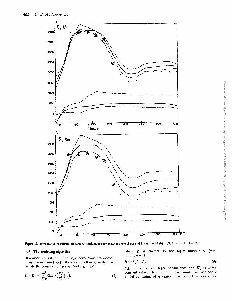
Figure 13. Distribution of calculated surface conductance for resultant model (a) and initial model (b). 1 ,2 ,3 , as for the Fig. 7.

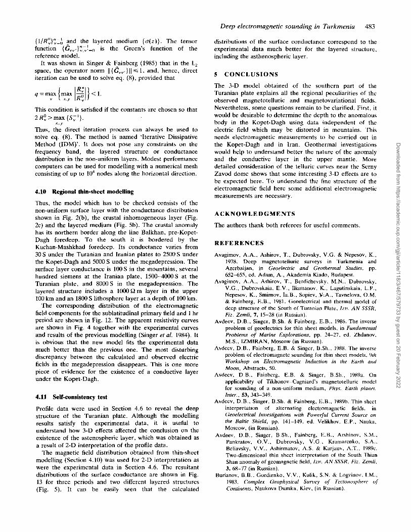
4.9 The modelling algorithm

If a model consists of n inhomogeneous layers embedded in a layered medium { a(z)}, then currents flowing in the layers satisfy the equation (Singer & Fainberg 1985):

where jSv is current in the layer number v (v =

R: = S;' - R"

S,,(x,y) is the vth layer conductance and R: is some constant value. The term 'reference model' is used for a model consisting of n uniform layers with conductances

0 , . . . , n - l ) ,

(9) V t

n-1

(8) fv = j;" - v ' = O

Dow




0 n-1 {1/Rv},,=(, 2nd the layered medium { ~ ( z ) } . The tensor function { G v v . } ~ ~ ! = O is the Green’s function of the reference model.

It was shown in Singer & Fainberg (1985) that in the (L,

space, the operator norm ~ ~ { & , , } ~ ~ s 1, and, hence, direct iteration can be used to solve eq. (8), provided that

q = m a x max 7 <1. v ( x . y IKy

This condition is satisfied if the constants are chosen so that 2 R : > max {S;’}.

Thus, the direct iteration process can always be used to solve eq. (8). The method is named ‘Iterative Dissipative Method (IDM)’. It does not pose any constraints on the frequency band, the layered structure or conductance distribution in the non-uniform layers. Modest performance computers can be used for modelling with a numerical mesh consisting of up to lo4 nodes along the horizontal direction.

X . Y

4.10 Regional thin-sheet modelling

Thus, the model which has to be checked consists of the non-uniform surface layer with the conductance distribution shown in Fig. 2(b), the crustal inhomogeneous layer (Fig. 2c) and the layered medium (Fig. 5b). The crustal anomaly has its northern border along the line Balkhan, pre-Kopet- Dagh foredeep. To the south it is bordered by the Kuchan-Mashkhad foredeep. Its conductance varies from 30 S under the Turanian and Iranian plates to 2500 S under the Kopet-Dagh and 5000 S under the megadepression. The surface layer conductance is 100 S in the mountains, several hundred siemens at the Iranian plate, 1500-4000s at the Turanian plate, and 8000s in the megadepression. The layered structure includes a 1000Qm layer in the upper 100 km and an 1800 S lithosphere layer at a depth of 100 km.

The corresponding distribution of the electromagnetic field components for the sublatitudinal primary field and 1 hr period are shown in Fig. 12. The apparent resistivity curves are shown in Fig. 4 together with the experimental curves and results of the previous modelling (Singer et al. 1984). It is obvious that the new model fits the experimental data much better than the previous one. The most disturbing discrepancy between the calculated and observed electric fields in the megadepression disappears. This is one more piece of evidence for the existence of a conductive layer under the Kopet-Dagh.

4.11 Self-consistency test

Profile data were used in Section 4.6 to reveal the deep structure of the Turanian plate. Although the modelling results satisfy the experimental data, it is useful to understand how 3-D effects affected the conclusion on the existence of the astenospheric layer, which was obtained as a result of 2-D interpretation of the profile data.

The magnetic field distribution obtained from thin-sheet modelling (Section 4.10) was used for 2-D interpretation as were the experimental data in Section 4.6. The resultant distributions of the surface conductance are shown in Fig. 13 for three periods and two different layered structures (Fig. 5). It can be easily seen that the calculated

distributions of the surtace conductance correspond to the experimental data much better for the layered structure, including the asthenospheric layer.

5 CONCLUSIONS

The 3-D model obtained of the southern part of the Turanian plate explains all the regional peculiarities of the observed magnetotelluric and magnetovariational fields. Nevertheless, some questions remain to be clarified. First, it would be desirable to determine the depth to the anomalous body in the Kopet-Dagh using data independent of the electric field which may be distorted in mountains. This needs electromagnetic measurements to be carried out in the Kopet-Dagh and in Iran. Geothermal investigations would help to understand better the nature of the anomaly and the conductive layer in the upper mantle. More detailed consideration of the telluric curves near the Serny Zavod dome shows that some interesting 3-D effects are to be expected here. To understand the fine structure of the electromagnetic field here some additional electromagnetic measurements are necessary.

ACKNOWLEDGMENTS

The authors thank both referees for useful comments.

REFERENCES

Avagimov, A.A., Ashirov, T., Dubrovsky, V.G. & Nepesov, K., 1978. Deep magnetotelluric surveys in Turkmenia and Azerbaijan, in Geoelectric and Geothermal Studies, pp. 652-655, ed. Adam, A., Akademia Kiado, Budapest.

Avagimov, A.A., Ashirov, T . , Berdichevsky, M.N., Dubrovsky, V.G., Dubrovskaia, E.V., Iliamanov, K., Lagutinskaia, L.P., Nepesov, K., Smirnov, Ia.B., Sopiev, .Y:A., Tavnelova. O.M. & Fainberg, E.B., 1981. Geoelectrical and thermal model of deep structure of the South of Turanian Plate, Izv. A N SSSR, Fiz. Zemli, 7, 15-28 (in Russian).

Avdeev, D.B., Singer, B.Sh. & Fainberg, E.B., 1986. The inverse problem of geoelectrics for thin sheet models, in Fundamental Problems of Marine Explorations, pp. 24-27. ed. Zhdanov, M.S., IZMIRAN, Moscow (in Russian).

Avdeev, D.B., Fainberg, E.B. & Singer, B.Sh., 1988. The inverse problem of electromagnetc sounding for thin sheet models, 9rh Workshop on Electromagnetic Induciion in the Earth and Moon, Abstracts, 50.

Avdeev, D.B., Fainberg, E.B. & Singer, B.Sh., 1989a. On applicability of Tikhonov-Cagniard’s magnetotelluric model for sounding of a non-uniform medium, Phvs. Earth planet. Inter.. 53, 343-349.

Avdeev, D.B., Singer, B.Sh. & Fainberg, E.B., 1989b. Thin sheet interpretation of alternating electromagnetic fields, in Geoelectrical Investigations with Powerful Current Source on the Baltic Shield, pp. 141-149. ed. Velikhov, E.P., Nauka, Moscow, (in Russian).

Avdeev, D.B., Singer, B.Sh., Fainberg, E.B.. Arshinov, S.M., Pankratov, O.V., Dubrovsky, V.G., Kramarenko, S.A., Beliavsky, V.V., Ashirmatov, A.S. & Karjauv, A.T., 1989~. Two-dimensional thin sheet interpretation of the South Thian Shan anomaly of geomagnetic field, Izu. A N SSSR, Fiz. Zernli, 3, 68-77 (in Russian).

Burianov, B.B., Gordienko, V.V., Kulik, S.N. & Logvinov, I.M., 1983. Complex Geophysical Survey of Teclonosphere of Continents, Naukova Dumka, Kiev, (in Russian).

Dow




Dawson, T. W. & Weaver, J.T., 1979. Three-dimensional electromagnetic induction in a non-uniform thin sheet at the surface of uniformly conducting earth, Geophys. J . R. astr. Soc., 59,445-462.

Egorkina, G.V., Krasnopevceva, G.V. & Schukin, U.K., 1980. Geophysical characteristics of the active zones, in Physical Processes in the Sources of Earthquakes, pp. 206-213, eds Sadovskij, M.A. & Myachkin, V.I., Nauka, Moscow, (in Russian).

Fainberg. E.B., 1983. Global and regional magnetovariational sounding, in Mathematical Modelling of Electromagnetic Fields, pp. 79-121, ed. Zhdanov, M.S., IZMIRAN, Moscow, (in Russian).

Gordienko, V.V. & Talvirskij, B.B. (eds), 1990. Tecionosphere of Middle Asia and South Kazakhstan, Naukova Dumka, Kiev, (in Russian).

Krasnopevtseva, G.S., 1988. The intermediate layer of the earth crust on the territory of the USSR in accordance with regional seismic data, in Geodynamic Explorations, Vol. 12, pp. 49-59, eds Byeloussov, V.V. & Karus, E.V., MGK, Moscow, (in Russian).

Kulik, S.N., Logvinov, I.M. & Gordienko, V.V., 1984. The crust conductors of Europe, in Crust Anomalies of Electroconductivity, pp. 41-48, ed. Zhamaletdinov, Nauka, Leningrad, (in Russian).

Lykov, V.I., Bezgodkov, V.A. & Orlov, V.S., 1975. The earth crust in Kopet-Dagh, Soviet Geol., 5, 126-129 (in Russian).

McKirdy, D.McA., Weaver, J.T. & Dawson, T.W., 1985. Induction in a thin sheet of variable conductance at the surface of a stratified earth-11. Three-dimensional theory, Geophys. J . R. asfr. SOC., 80, 177-194.

Nikolaevskij. V.N., 1986. Delatancy rheology of the lithosphere and waves of the tectonic tensions, in Basic Problems of Seismotectonics, pp. 51-68, ed. Shchukin Yu, K., Nauka, Moscow, (in Russian).

Rezanov, LA., 1980. On the geological interpretation of the new

three layered seismic model of contents, Izv. AN SSSr, Fiz. Zemli, 9, 79-86 (in Russian).

Riaboj, V.Z., 1975. The structure of the Earth crust and upper mantle along profile of deep seismic sounding Kopet-Dagh- Aral sea, Soviet Geol., 5 , 79-86, (in Russian).

Raiboj, V.Z. & Matushkin, B.A., 1969. To question on joint using of gravimetric, magnetic and deep seismic methods for investigations of earth crust and upper mantle (an example of Central Turkmenia and southern pre-Aral), in Methodology and Results of Complex Geophysical Investigations, pp. 151-158, ed. Volfovsky, I.S., Nedra, Leningrad, (in Russian).

Schmucker, U., 1971. Interpretation of inductive anomalies above non-uniform surface layer, Geophysics, 36, 156-165.

Shteklin, Dg., 1966. Tectonics of Iran, Geotectonics, N1, 3-21 (in Russian).

Singer, B.Sh. & Fainberg, E.G., 1985. Electromagnetic Induction in Non-uniform Thin Layers, IZMIRAN, Moscow.

Singer, B.Sh., Dubrovsky, V.G., Fainberg, E.B., Berdichevsky, M.N. & Iliamanov, K., 1984. The quasi three dimensional modelling of magnetotelluric fields at the South of Turanian Plate and in the South Caspian Megadepression, Izv. AN SSSR, Fiz. Zemli, 1, 69-81 (in Russian).

Vanyan, L.L., 1984. Electroconductivity of the earth crust in connection with its fluid regime, in Crusr Anomalies of Electroconductance, pp. 27-40, ed. Zhamaletdinov, A.A., Nauka, Leningrad, (in Russian).

Vanyan, L.L., Dubrovsky, V.G., Yegorov, I.V. & Konnov, U.K., 1983. Structure of the low frequency telluric field in the South Caspian Megadepression in accordance with the numerical modelling, Izv. A N SSSR, Fiz. Zemli, 7 , 98-101 (in Russian).

Zhamaletdinov, A. A., 1990. The Model of Electrical Conductivity of Asthenosphere According to the Results of Investigations with Control Sources of Field, Nauka, Leningrad, (in Russian).

Zvereva, S.M. & Kosminskaya, I.P. (eds), 1980. Geoelectrical and Thermal Model of the Basic Geological Structures of USSR, Nauka, Moscow (in Russian).

Dow



Documents

Deep electromagnetic sounding in Turkmenia - Geophysical Journal