Embed Size (px)
Citation preview
Imperial College London
Department of Computing
Deep Convolutional Neural Networks for Smile
Recognition
Patrick Oliver GLAUNER
September 2015
Supervised by Professor Maja PANTIC
and Dr. Stavros PETRIDIS
Submitted in part fulfilment of the requirements for the degree of
Master of Science in Computing (Machine Learning) of Imperial College London
1
arX
iv:1
508.
0653
5v1
[cs
.CV
] 2
6 A
ug 2
015

Declaration
I herewith certify that all material in this report which is not my own work has been properly acknow-
ledged.
Patrick Oliver GLAUNER
2
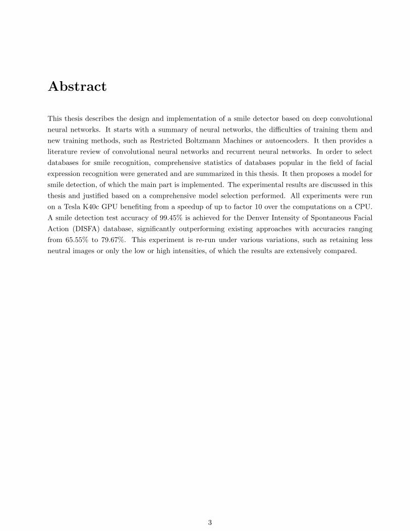
Abstract
This thesis describes the design and implementation of a smile detector based on deep convolutional
neural networks. It starts with a summary of neural networks, the difficulties of training them and
new training methods, such as Restricted Boltzmann Machines or autoencoders. It then provides a
literature review of convolutional neural networks and recurrent neural networks. In order to select
databases for smile recognition, comprehensive statistics of databases popular in the field of facial
expression recognition were generated and are summarized in this thesis. It then proposes a model for
smile detection, of which the main part is implemented. The experimental results are discussed in this
thesis and justified based on a comprehensive model selection performed. All experiments were run
on a Tesla K40c GPU benefiting from a speedup of up to factor 10 over the computations on a CPU.
A smile detection test accuracy of 99.45% is achieved for the Denver Intensity of Spontaneous Facial
Action (DISFA) database, significantly outperforming existing approaches with accuracies ranging
from 65.55% to 79.67%. This experiment is re-run under various variations, such as retaining less
neutral images or only the low or high intensities, of which the results are extensively compared.
3

First and foremost I offer my sincerest gratitude to my supervisor Dr. Stavros
PETRIDIS who has supported me throughout my thesis with his enthusiasm,
patience and expertise.
I would also like to thank Professor Maja PANTIC for her passion, setting the
direction of this thesis and valuable regular feedback.
Furthermore, I am eternally obliged to the feedback and advice on neural
networks from Professor Sinisa TODOROVIC.
4
Contents
1. Introduction 12
2. Background report: neural networks 13
2.1. Feed-forward neural networks . . . . . . . . . . . . . . . . . . . . . . . . . . . . . . . . . 13
2.1.1. Difficulty of training . . . . . . . . . . . . . . . . . . . . . . . . . . . . . . . . . . 14
2.2. Deep neural networks . . . . . . . . . . . . . . . . . . . . . . . . . . . . . . . . . . . . . 15
2.2.1. Training methods . . . . . . . . . . . . . . . . . . . . . . . . . . . . . . . . . . . . 16
2.2.2. Activation functions . . . . . . . . . . . . . . . . . . . . . . . . . . . . . . . . . . 16
2.2.3. Application to facial expression data . . . . . . . . . . . . . . . . . . . . . . . . . 17
2.3. Recurrent neural networks . . . . . . . . . . . . . . . . . . . . . . . . . . . . . . . . . . . 17
2.3.1. Long short-term memory . . . . . . . . . . . . . . . . . . . . . . . . . . . . . . . 17
2.4. Convolutional neural networks . . . . . . . . . . . . . . . . . . . . . . . . . . . . . . . . 19
2.5. Processing of image sequences . . . . . . . . . . . . . . . . . . . . . . . . . . . . . . . . . 20
3. Selection of databases 24
3.1. FACS coding . . . . . . . . . . . . . . . . . . . . . . . . . . . . . . . . . . . . . . . . . . 24
3.2. Available databases . . . . . . . . . . . . . . . . . . . . . . . . . . . . . . . . . . . . . . . 24
3.3. Distribution of action unit intensities . . . . . . . . . . . . . . . . . . . . . . . . . . . . . 25
3.4. Selected databases . . . . . . . . . . . . . . . . . . . . . . . . . . . . . . . . . . . . . . . 26
3.4.1. DISFA . . . . . . . . . . . . . . . . . . . . . . . . . . . . . . . . . . . . . . . . . . 27
3.4.2. Others . . . . . . . . . . . . . . . . . . . . . . . . . . . . . . . . . . . . . . . . . . 28
4. Model 29
4.1. Proposed model . . . . . . . . . . . . . . . . . . . . . . . . . . . . . . . . . . . . . . . . . 29
4.2. Implementation . . . . . . . . . . . . . . . . . . . . . . . . . . . . . . . . . . . . . . . . . 30
4.2.1. Selection of deep learning library . . . . . . . . . . . . . . . . . . . . . . . . . . . 30
4.2.2. Selection of LSTM library . . . . . . . . . . . . . . . . . . . . . . . . . . . . . . . 31
4.2.3. Progress of implementation . . . . . . . . . . . . . . . . . . . . . . . . . . . . . . 31
4.3. Computing infrastructure . . . . . . . . . . . . . . . . . . . . . . . . . . . . . . . . . . . 31
5. Towards a static convolutional smile detector 33
5.1. Selected parameters and assumptions . . . . . . . . . . . . . . . . . . . . . . . . . . . . . 33
5.1.1. Candidate parameters to be optimized . . . . . . . . . . . . . . . . . . . . . . . . 33
5.1.2. Selected parameters and values . . . . . . . . . . . . . . . . . . . . . . . . . . . . 34
5.1.3. Cost function and performance metrics . . . . . . . . . . . . . . . . . . . . . . . . 35
5

5.1.4. Input size . . . . . . . . . . . . . . . . . . . . . . . . . . . . . . . . . . . . . . . . 35
5.2. Bottom lines . . . . . . . . . . . . . . . . . . . . . . . . . . . . . . . . . . . . . . . . . . 36
5.3. Model selection for full dataset . . . . . . . . . . . . . . . . . . . . . . . . . . . . . . . . 36
5.3.1. Mouth . . . . . . . . . . . . . . . . . . . . . . . . . . . . . . . . . . . . . . . . . . 37
5.3.2. Face . . . . . . . . . . . . . . . . . . . . . . . . . . . . . . . . . . . . . . . . . . . 38
5.3.3. Comparison of mouth vs. face . . . . . . . . . . . . . . . . . . . . . . . . . . . . . 38
5.4. Model selection for reduced dataset . . . . . . . . . . . . . . . . . . . . . . . . . . . . . . 38
5.4.1. Mouth . . . . . . . . . . . . . . . . . . . . . . . . . . . . . . . . . . . . . . . . . . 39
5.4.2. Face . . . . . . . . . . . . . . . . . . . . . . . . . . . . . . . . . . . . . . . . . . . 39
5.4.3. Comparison of mouth vs. face . . . . . . . . . . . . . . . . . . . . . . . . . . . . . 39
5.5. Repeatability of experiments . . . . . . . . . . . . . . . . . . . . . . . . . . . . . . . . . 40
5.6. Evaluation of final models for full and reduced datasets . . . . . . . . . . . . . . . . . . 40
5.7. Comparison of low and high intensities for reduced dataset . . . . . . . . . . . . . . . . 43
5.8. Classification of low and high intensities . . . . . . . . . . . . . . . . . . . . . . . . . . . 46
6. Conclusions and future work 48
Bibliography 49
A. Statistics of all action units 54
B. Training time of networks 57
B.1. Full dataset . . . . . . . . . . . . . . . . . . . . . . . . . . . . . . . . . . . . . . . . . . . 57
B.2. Reduced dataset . . . . . . . . . . . . . . . . . . . . . . . . . . . . . . . . . . . . . . . . 58
B.3. Low and high intensities for reduced dataset . . . . . . . . . . . . . . . . . . . . . . . . . 58
B.4. Classification of low and high intensities . . . . . . . . . . . . . . . . . . . . . . . . . . . 59
C. Result of model selection 60
C.1. Full dataset . . . . . . . . . . . . . . . . . . . . . . . . . . . . . . . . . . . . . . . . . . . 60
C.2. Reduced dataset . . . . . . . . . . . . . . . . . . . . . . . . . . . . . . . . . . . . . . . . 60
D. Performance of selected models 64
D.1. Full dataset . . . . . . . . . . . . . . . . . . . . . . . . . . . . . . . . . . . . . . . . . . . 64
D.2. Reduced dataset . . . . . . . . . . . . . . . . . . . . . . . . . . . . . . . . . . . . . . . . 64
6
List of Tables
3.1. Selected statistics of action units in databases: an integer denotes the number of frames
in which an action unit is set (intensity > 0). A hyphen indicates that an action unit is
not available in a database. . . . . . . . . . . . . . . . . . . . . . . . . . . . . . . . . . . 27
3.2. Distribution of AU12 in DISFA. . . . . . . . . . . . . . . . . . . . . . . . . . . . . . . . . 28
5.1. Parameters and possible values used in model selection. . . . . . . . . . . . . . . . . . . 35
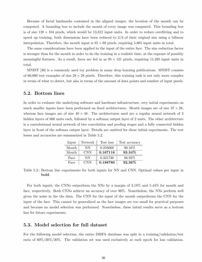
5.2. Bottom line experiments for both inputs for NN and CNN. Optimal values per input in
bold. . . . . . . . . . . . . . . . . . . . . . . . . . . . . . . . . . . . . . . . . . . . . . . 36
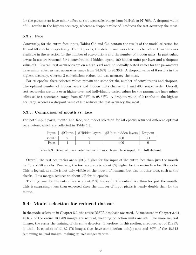
5.3. Selected parameter values for mouth and face input. For full dataset. . . . . . . . . . . . 38
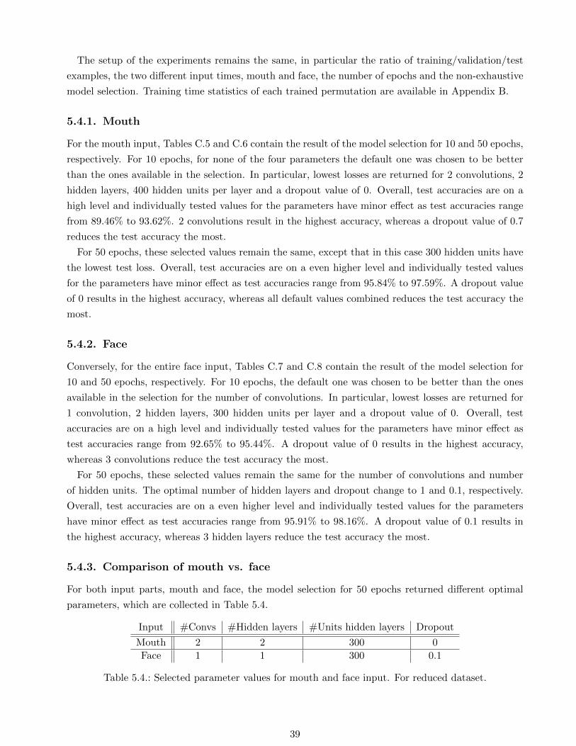
5.4. Selected parameter values for mouth and face input. For reduced dataset. . . . . . . . . 39
5.5. Repeatability of training of architecture with default values and 2 hidden layers for
mouth for 50 epochs: standard deviation of test accuracies. Optimal values in bold.
For full dataset. . . . . . . . . . . . . . . . . . . . . . . . . . . . . . . . . . . . . . . . . . 40
5.6. Result of model selection for mouth and face with the combined parameters for selected
epochs. Optimal values per part in bold. For full dataset. . . . . . . . . . . . . . . . . . 41
5.7. Result of model selection for mouth and face with the combined parameters for selected
epochs. Optimal values per part in bold. For reduced dataset. . . . . . . . . . . . . . . 42
5.8. Parameter values for mouth and face input for low and high intensity models. . . . . . . 43
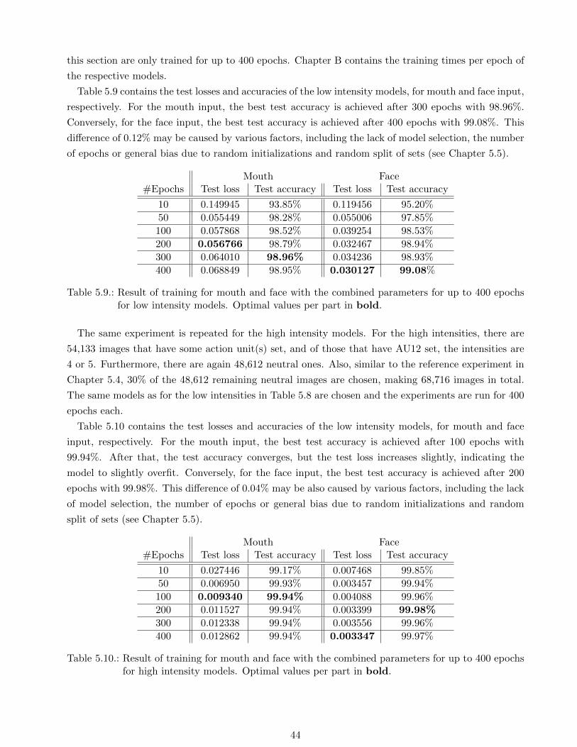
5.9. Result of training for mouth and face with the combined parameters for up to 400 epochs
for low intensity models. Optimal values per part in bold. . . . . . . . . . . . . . . . . . 44
5.10. Result of training for mouth and face with the combined parameters for up to 400 epochs
for high intensity models. Optimal values per part in bold. . . . . . . . . . . . . . . . . 44
5.11. Result of training for mouth and face with the combined parameters for up to 400 epochs
for classification of low and high intensities. Optimal values per part in bold. . . . . . . 47
A.1. Complete statistics of action units in databases: an integer denotes the number of frames
in which an action unit is set (intensity > 0). A hyphen indicates that an action unit is
not available in a database. . . . . . . . . . . . . . . . . . . . . . . . . . . . . . . . . . . 56
B.1. Median epoch duration in seconds during model selection of different architectures. For
full dataset. . . . . . . . . . . . . . . . . . . . . . . . . . . . . . . . . . . . . . . . . . . . 57
B.2. Median epoch duration in seconds for final models selected. For full dataset. . . . . . . . 57
B.3. Median epoch duration in seconds during model selection of different architectures. For
reduced dataset. . . . . . . . . . . . . . . . . . . . . . . . . . . . . . . . . . . . . . . . . 58
B.4. Median epoch duration in seconds for final models selected. For reduced dataset. . . . . 58
7
B.5. Median epoch duration in seconds for models for low intensities. For reduced dataset. . 58
B.6. Median epoch duration in seconds for models for high intensities. For reduced dataset. . 58
B.7. Median epoch duration in seconds for models for classification of low and high intensities. 59
C.1. Model selection for mouth for 10 epochs. Optimal values per parameter in bold. For
full dataset. . . . . . . . . . . . . . . . . . . . . . . . . . . . . . . . . . . . . . . . . . . . 60
C.2. Model selection for mouth for 50 epochs. Optimal values per parameter in bold. For
full dataset. . . . . . . . . . . . . . . . . . . . . . . . . . . . . . . . . . . . . . . . . . . . 61
C.3. Model selection for face for 10 epochs. Optimal values per parameter in bold. For full
dataset. . . . . . . . . . . . . . . . . . . . . . . . . . . . . . . . . . . . . . . . . . . . . . 61
C.4. Model selection for face for 50 epochs. Optimal values per parameter in bold. For full
dataset. . . . . . . . . . . . . . . . . . . . . . . . . . . . . . . . . . . . . . . . . . . . . . 61
C.5. Model selection for mouth for 10 epochs. Optimal values per parameter in bold. For
reduced dataset. . . . . . . . . . . . . . . . . . . . . . . . . . . . . . . . . . . . . . . . . 62
C.6. Model selection for mouth for 50 epochs. Optimal values per parameter in bold. For
reduced dataset. . . . . . . . . . . . . . . . . . . . . . . . . . . . . . . . . . . . . . . . . 62
C.7. Model selection for face for 10 epochs. Optimal values per parameter in bold. For
reduced dataset. . . . . . . . . . . . . . . . . . . . . . . . . . . . . . . . . . . . . . . . . 62
C.8. Model selection for face for 50 epochs. Optimal values per parameter in bold. For
reduced dataset. . . . . . . . . . . . . . . . . . . . . . . . . . . . . . . . . . . . . . . . . 63
D.1. Result of model selection for mouth and face with the combined parameters for 10, 100,
200, ..., 1000 epochs. Optimal values per part in bold. For full dataset. . . . . . . . . . 64
D.2. Result of model selection for mouth and face with the combined parameters for 10, 100,
200, ..., 1000 epochs. Optimal values per part in bold. For reduced dataset. . . . . . . . 65
8
List of Figures
2.1. Neural network with two input and output units and one hidden layer with two units
and bias units x0 and z0 [4]. . . . . . . . . . . . . . . . . . . . . . . . . . . . . . . . . . . 13
2.2. Deep neural network layers learning complex feature hierarchies [56]. . . . . . . . . . . . 15
2.3. Sigmoid and ReLU activation functions. . . . . . . . . . . . . . . . . . . . . . . . . . . . 16
2.4. Simple recurrent neural network with one recurrent connection from the hidden layer to
the input layer in bold. . . . . . . . . . . . . . . . . . . . . . . . . . . . . . . . . . . . . 17
2.5. LSTM cell: the integral sign stands for the Sigmoid function, the large filled dot for a
multiplication [21]. . . . . . . . . . . . . . . . . . . . . . . . . . . . . . . . . . . . . . . . 18
2.6. Example LSTM network: eight input units, four output units, and two memory cell
blocks of size two [21]. . . . . . . . . . . . . . . . . . . . . . . . . . . . . . . . . . . . . . 18
2.7. Illustration of a convolutional neural network [4]. . . . . . . . . . . . . . . . . . . . . . . 19
2.8. Multiple convolutions to process video input [27]. . . . . . . . . . . . . . . . . . . . . . . 20
2.9. Deep neural network composed of convolutions, LSTMs, dimensionality reduction and
regular layers [49]. . . . . . . . . . . . . . . . . . . . . . . . . . . . . . . . . . . . . . . . 21
2.10. Fusion of low-resolution with higher-resolution of the center of the video [27]. . . . . . . 22
2.11. Fusion of low-resolution with optical flow [42]. . . . . . . . . . . . . . . . . . . . . . . . . 22
2.12. Final stage done by SVM instead of neural network [26]. . . . . . . . . . . . . . . . . . . 23
3.1. Sample images of the DISFA database [35]. . . . . . . . . . . . . . . . . . . . . . . . . . 25
3.2. Binary statistics of CASME database. . . . . . . . . . . . . . . . . . . . . . . . . . . . . 25
3.3. Intensity statistics for video 002 of DISFA database. Left subplot: all intensities, right
subplot: all positive intensities. . . . . . . . . . . . . . . . . . . . . . . . . . . . . . . . . 26
3.4. Intensity statistics for all videos of DISFA database. Left subplot: all intensities, right
subplot: all positive intensities. . . . . . . . . . . . . . . . . . . . . . . . . . . . . . . . . 26
3.5. Sample image of aligned DISFA database of size 285× 378 pixels [35]. . . . . . . . . . . 27
4.1. Proposed model. . . . . . . . . . . . . . . . . . . . . . . . . . . . . . . . . . . . . . . . . 30
4.2. Examples of speedups using Tesla graphic card series [45]. . . . . . . . . . . . . . . . . . 32
4.3. Output of nvidia-smi for sample experiment. . . . . . . . . . . . . . . . . . . . . . . . 32
5.1. Different input parts: a) mouth, b) face [35]. (Not at actual input size/proportions.) . . 35
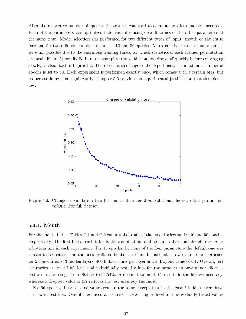
5.2. Change of validation loss for mouth data for 2 convolutional layers, other parameters
default. For full dataset. . . . . . . . . . . . . . . . . . . . . . . . . . . . . . . . . . . . . 37
5.3. Change of test accuracy for mouth and face data over 1000 epochs. For full dataset. . . 41
5.4. Change of test accuracy for mouth and face data over 1000 epochs. For reduced dataset. 42
9

5.5. Change of test accuracy for mouth and face data over 1000 epochs. For both datasets. . 43
5.6. DISFA examples of video 002 for no smile, low intensity smile and high intensity smile
[35]. . . . . . . . . . . . . . . . . . . . . . . . . . . . . . . . . . . . . . . . . . . . . . . . 45
5.7. DISFA examples of video 005 for no smile, low intensity smile and high intensity smile
[35]. . . . . . . . . . . . . . . . . . . . . . . . . . . . . . . . . . . . . . . . . . . . . . . . 45
5.8. DISFA examples of video 023 for no smile, low intensity smile and high intensity smile
[35]. . . . . . . . . . . . . . . . . . . . . . . . . . . . . . . . . . . . . . . . . . . . . . . . 46
10
List of Algorithms
2.1. Backpropagation: training size m. . . . . . . . . . . . . . . . . . . . . . . . . . . . . . . 14
2.2. Batch gradient descent: training size m, learning rate α. . . . . . . . . . . . . . . . . . . 14
2.3. Stochastic gradient descent: training size m, learning rate α. . . . . . . . . . . . . . . . 15
11
1. Introduction
Neural networks have been popular in the machine learning community since the 1980s with repeating
rises and falls of popularity. Their main benefit is their ability to learn complex, non-linear hypotheses
from data without the need of modeling complex features. This makes them of particular interest
for computer vision, in which feature description is a long-standing and largely non-understood topic.
Neural networks are difficult to train and for the last ten years they have come to enormous fame
under the topic ”deep learning”. New advances in training methods and the movement of training from
CPUs to GPUs allow to train more reliable models much faster. Deep neural networks are not a silver
bullet, as training is still heavily based on model selection and experimentation. Overall, significant
progress in machine learning and pattern recognition has been made in natural language processing,
computer vision and audio processing. Leading IT companies have made significant investments into
deep learning for these reasons, such as Baidu, Google, Facebook and Microsoft.
Concretely, previous work of the author on deep learning for facial expression recognition in [12]
resulted in a deep neural network model that significantly outperformed the best contribution to the
2013 Kaggle facial expression competition [25]. Therefore, a further investigation on the recognition
of action units and in particular smile using deep neural networks and convolutional neural networks
seems desirable. Only very few works on this topic have been reported so far, such as in [16]. It would
also be interesting to compare the input of the entire face versus the mouth to study differences in the
performance of deep convolutional models.
12
2. Background report: neural networks
This chapter provides an overview of different types of neural networks, their capabilities and training
challenges, based on [12]. This chapter does not provide an introduction to neural networks, the reader
is therefore referred to [4] and [37] for a comprehensive introduction to neural neural networks.
Neural networks are inspired by the brain and composed of multiple layers of logistic regression
units, called neurons. They experienced different periods of hypes in the 1960s and 1980s/90s. Neural
networks are known to be able to learn complex hypotheses for regression and classification. Conversely,
training neural networks is difficult, as their cost functions have many local minima. Hence, training
tends to converge to a local minimum, resulting in poor generalization of the network. For the last
ten years, neural networks have been celebrating a comeback under the term deep learning, taking
advantage of many hidden layers in order to build more powerful machine learning algorithms.
2.1. Feed-forward neural networks
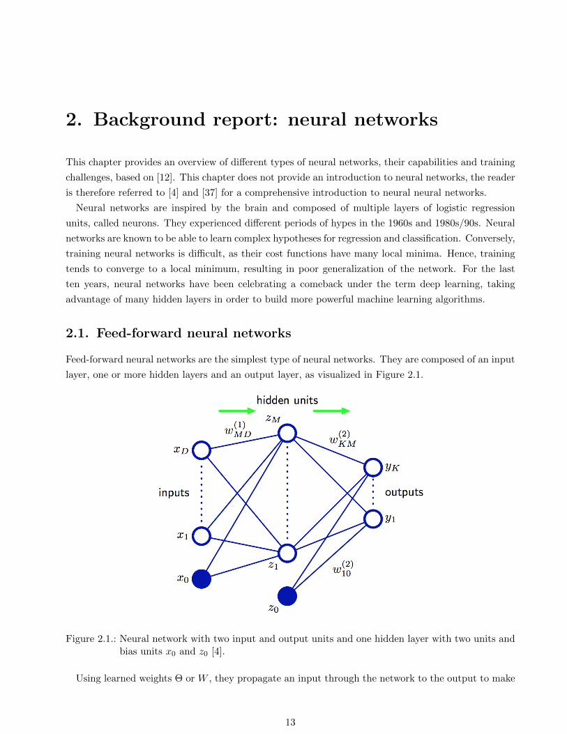
Feed-forward neural networks are the simplest type of neural networks. They are composed of an input
layer, one or more hidden layers and an output layer, as visualized in Figure 2.1.
Figure 2.1.: Neural network with two input and output units and one hidden layer with two units andbias units x0 and z0 [4].
Using learned weights Θ or W , they propagate an input through the network to the output to make
13
predictions. The activation of unit i of layer j + 1 can be calculated as follows:
z(j+1)i =
sj∑k=0
Θ(j)ik xk (2.1)
a(j+1)i = g
(z
(j+1)i
)(2.2)
g is an activation function, for which often the Sigmoid activation function 11+e−x is used in the hidden
layers. The Sigmoid function or its generalization, the softmax function, are used for classification
problems in the output layer units. For regression problems, the sum of Equation 2.1 is used directly
in the output layer without the use of any activation functions.
In order to learn the weights, a cost function is minimized. There are different cost functions, such
as the least squares or cross-entropy cost function, described in [37]. The latter one has been reported
to generalize better and speed up learning as discussed in [40].
2.1.1. Difficulty of training
In order to learn the weights, Algorithm 2.1 named backpropagation is used to efficiently compute
the partial derivatives, which are then fed into an optimization algorithm, such as gradient descent
(Algorithm 2.2) or stochastic gradient descent (Algorithm 2.3), as described in [31]. Those three
algorithms are based on [40].
Algorithm 2.1 Backpropagation: training size m.
Θ(l)ij ← rand(−ε, ε) (for all l, i, j)
∆(l)ij ← 0 (for all l, i, j)
for i = 1 to m do
a(1) ← x(i)
Perform forward propagation to compute a(l) for l = 2, 3, ..., L
Using y(i), compute δ(L) = a(L) − y(i) . ”error”
Compute δ(L−1), δ(L−2), ..., δ(2): δ(l) = (Θ(l))T δ(l+1) ◦ g′(z(l))
∆(l) ← ∆(l) + δ(l+1)(a(l))T . Matrix of errors for units of a layer
end for∂
∂Θ(l)ij
J(Θ)← 1m∆
(l)ij
Algorithm 2.2 Batch gradient descent: training size m, learning rate α.
repeat
θj ← θj − α ∂∂θjJ(θ) (simultaneously for all j)
until convergence
Generally, the more units in a neural network, the higher its expressional complexity. In contrast,
the more units, the more it tends to overfit. To prevent overfitting, various approaches have been
14
Algorithm 2.3 Stochastic gradient descent: training size m, learning rate α.
Randomly shuffle data setrepeat
for i = 1 to m doθj ← θj − α ∂
∂θjJ(θ, (x(i), y(i))) (simultaneously for all j)
end foruntil convergence
described in the literature, including L1/L2 regularization [39], early stopping, tangent propagation [4]
and dropout [53].
2.2. Deep neural networks
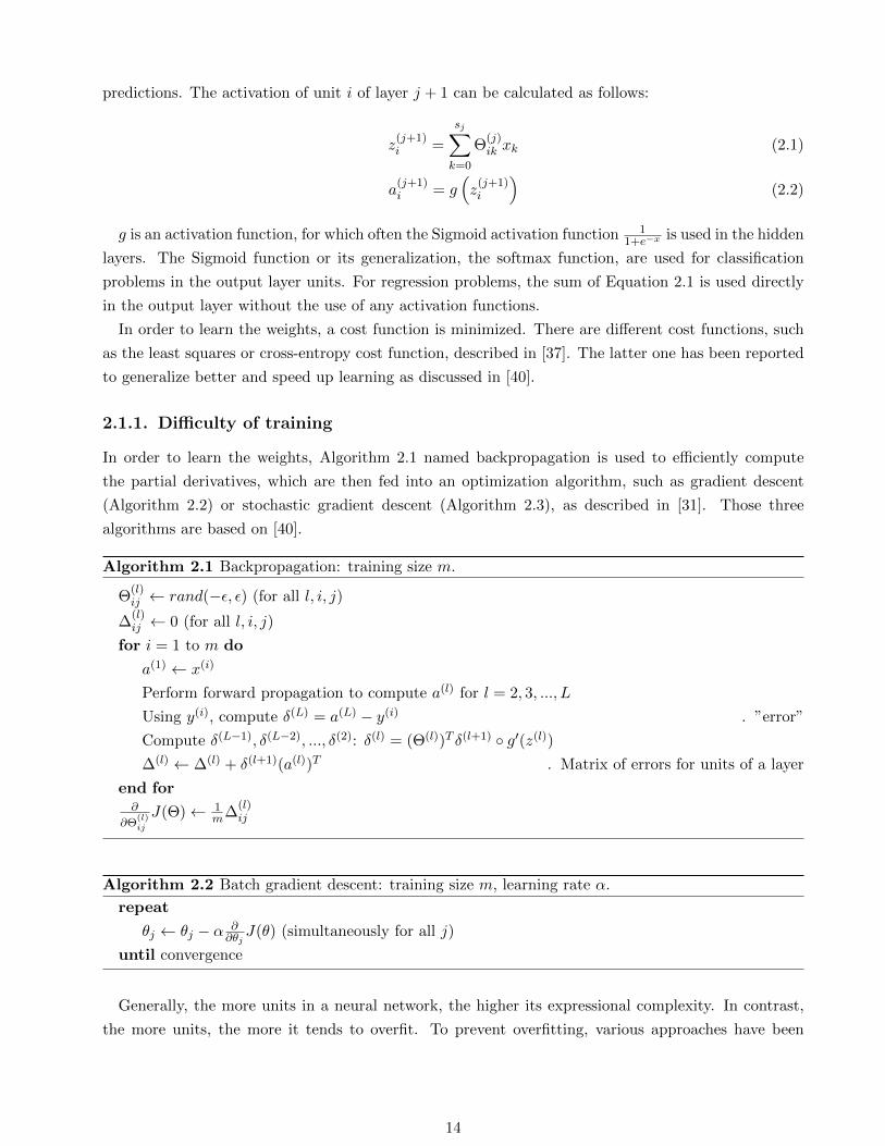
Deep neural networks use many hidden layers. This allows to learn increasingly more complex features
hierarchies, as visualized in Figure 2.2 for the Google Brain [29]. Such architectures are of enormous
benefit, as the long-standing problem of feature description in signal processing disappears to a large
extend.
Figure 2.2.: Deep neural network layers learning complex feature hierarchies [56].
Conversely, training of deep neural networks gets more difficult because of the increased number
of parameters. As described in [7] and [8], backpropagation does not scale to deep neural networks:
starting with small random initial weights, the backpropagated partial derivatives go towards zero. As
a result, training becomes infeasible and is called the vanishing gradient problem.
15
2.2.1. Training methods
For deep neural networks, training has therefore been split in two parts: pre-training and fine-tuning.
Pre-training allows to initialize the weights to a location in the cost function which can be optimized
quickly using regular backpropagation.
Various pre-training methods have been described in the literature. Most prominently, unsupervised
methods, such as Restricted Boltzmann Machines (RBM) in [18] and [20] or autoencoders in [41] and
[5] are used. Both methods learn exactly one hidden layer. This hidden layer is then used as input to
the next RBM or autoencoder to learn the next hidden layer. This process can be repeated for many
times in order to pre-train a so-called Deep Belief Network (DBN) or Stacked Autoencoder, composed
of RBMs or autoencoders respectively. In addition, there are denoising autoencoders defined in [28],
which are autoencoders that are trained to denoise corrupted inputs. Furthermore, other methods such
as discriminative pre-training [19] or reduction of internal covariance shift [22] have been reported as
effective training methods for deep neural networks.
2.2.2. Activation functions
In the past, mostly Sigmoid units have been used in the hidden layers, with Sigmoid or linear units in
the output layer for classification or regression, respectively. For classification, the softmax activation
is preferred in the output layer. As described by Norvig in [44], the output of a set unit is much
stronger than the others. Another benefit of softmax is that it is always differentiable for a weight.
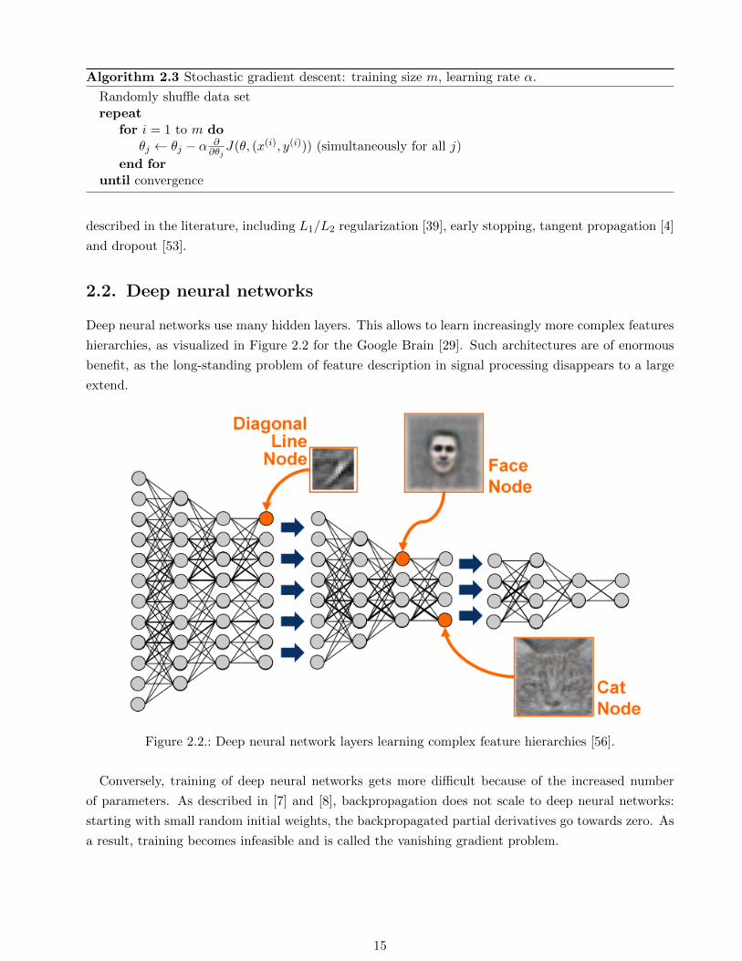
Recently, the so-called rectified linear unit (ReLU) has been proposed in [38], which has been used
successfully in many deep learning applications. Figure 2.3 visualizes the Sigmoid and ReLU functions.
Figure 2.3.: Sigmoid and ReLU activation functions.
ReLU has a number of advantages over Sigmoid, reported in [38] and [14]. First, it is much easier to
16
compute as it is either 0 or the input value. Also, Sigmoid has for non-activated input values less than
or equal to 0 an activation value of greater than 0. In contrast, ReLU models biological behavior of
neurons more accurately, as it is 0 for those cases. With many units set to 0, a sparse activation of the
networks follows, which is another form of regularization. Furthermore, the vanishing gradient problem
becomes less of an issue as ReLU units result in a simpler cost function. Last, for some experiments,
ReLU reduces the importance of pre-training or may not be necessary at all.
2.2.3. Application to facial expression data
In the context of this project, deep neural networks have been successfully applied to facial expression
recognition in [12]. In that study, RBMs, autoencoders and denoising autoencoders were compared
on a noisy dataset from a 2013 Kaggle challenge named ”Emotion and identity detection from face
images” [25]. This challenge was won by a neural network presented in [55], which achieved an error
rate of 52.977%. In [12], a stacked autoencoder was trained with an error of 39.75%. In a subsequent
project, this error could be reduced further to 28% with a stacked denoising autoencoder [13]. This
study also showed that deep neural networks are a promising machine learning method for this context,
but not a silver bullet as data pre-processing and intensive model selection are still required.
2.3. Recurrent neural networks
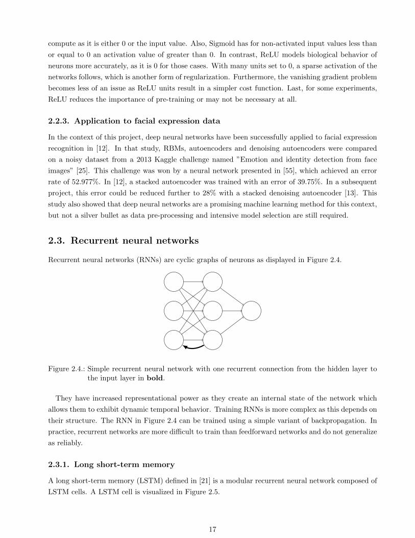
Recurrent neural networks (RNNs) are cyclic graphs of neurons as displayed in Figure 2.4.
Figure 2.4.: Simple recurrent neural network with one recurrent connection from the hidden layer tothe input layer in bold.
They have increased representational power as they create an internal state of the network which
allows them to exhibit dynamic temporal behavior. Training RNNs is more complex as this depends on
their structure. The RNN in Figure 2.4 can be trained using a simple variant of backpropagation. In
practice, recurrent networks are more difficult to train than feedforward networks and do not generalize
as reliably.
2.3.1. Long short-term memory
A long short-term memory (LSTM) defined in [21] is a modular recurrent neural network composed of
LSTM cells. A LSTM cell is visualized in Figure 2.5.
17
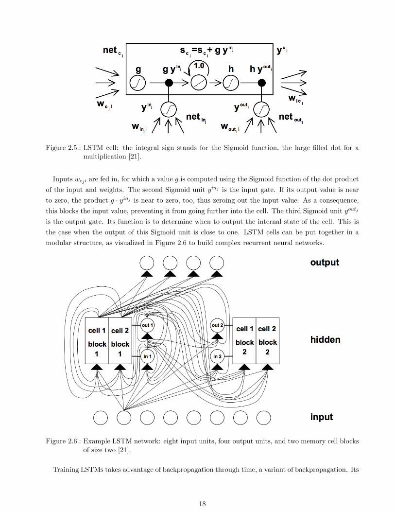
Figure 2.5.: LSTM cell: the integral sign stands for the Sigmoid function, the large filled dot for amultiplication [21].
Inputs wcji are fed in, for which a value g is computed using the Sigmoid function of the dot product
of the input and weights. The second Sigmoid unit yinj is the input gate. If its output value is near
to zero, the product g · yinj is near to zero, too, thus zeroing out the input value. As a consequence,
this blocks the input value, preventing it from going further into the cell. The third Sigmoid unit youtj
is the output gate. Its function is to determine when to output the internal state of the cell. This is
the case when the output of this Sigmoid unit is close to one. LSTM cells can be put together in a
modular structure, as visualized in Figure 2.6 to build complex recurrent neural networks.
Figure 2.6.: Example LSTM network: eight input units, four output units, and two memory cell blocksof size two [21].
Training LSTMs takes advantage of backpropagation through time, a variant of backpropagation. Its
18
goal is to minimize the LSTM’s total cost on a training set. LSTMs have been reported to outperform
regular RNNs and Hidden Markov Models in classification and time series prediction tasks. LSTMs
have also been reported in [54] to perform well on prediction of image sequences.
2.4. Convolutional neural networks
Invariance to transformations is a desired property of learning algorithms. Typical variances of im-
ages and videos include translation, rotation and scaling. Tangent propagation [4] is one method in
neural networks to handle transformations by penalizing the amount of distortion in the cost func-
tion. Convolutional neural networks (CNNs) are a different approach to implementing invariance in
neural networks, which are inspired by biological processes. CNNs were initially proposed by LeCun
in [30]. They have been successfully applied to computer vision problems, such as hand-written digit
recognition.
In images, nearby pixels are strongly correlated, a property of which local features take advantage
of. In a hierarchical approach, local features are used in the first stage of pattern recognition, allowing
recognition of more complex features.
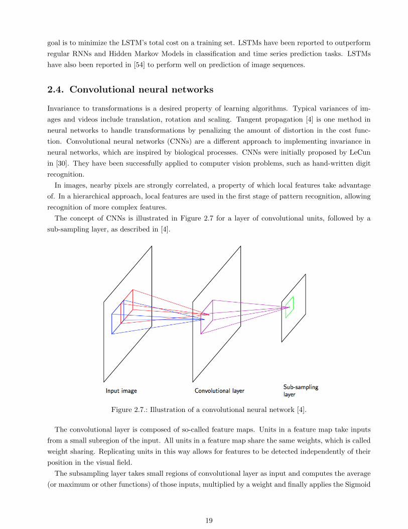
The concept of CNNs is illustrated in Figure 2.7 for a layer of convolutional units, followed by a
sub-sampling layer, as described in [4].
Figure 2.7.: Illustration of a convolutional neural network [4].
The convolutional layer is composed of so-called feature maps. Units in a feature map take inputs
from a small subregion of the input. All units in a feature map share the same weights, which is called
weight sharing. Replicating units in this way allows for features to be detected independently of their
position in the visual field.
The subsampling layer takes small regions of convolutional layer as input and computes the average
(or maximum or other functions) of those inputs, multiplied by a weight and finally applies the Sigmoid
19
function to the value. The result of a unit in the subsampling layer is relatively insensitive to small
shifts or rotations of the image in the corresponding regions of the input space. This concept can be
repeated for more times to subsequently be more invariant and to detect more complex features.
Because of the constraints of weights, the number of independent parameters in the network is
smaller than in a fully-connected network. This allows to train the network faster and to be less prone
to overfitting. Training of CNNs requires minimization of a cost function. The idea of backpropagation
can be applied to CNN with a small modification taking into account the weight sharing.
2.5. Processing of image sequences
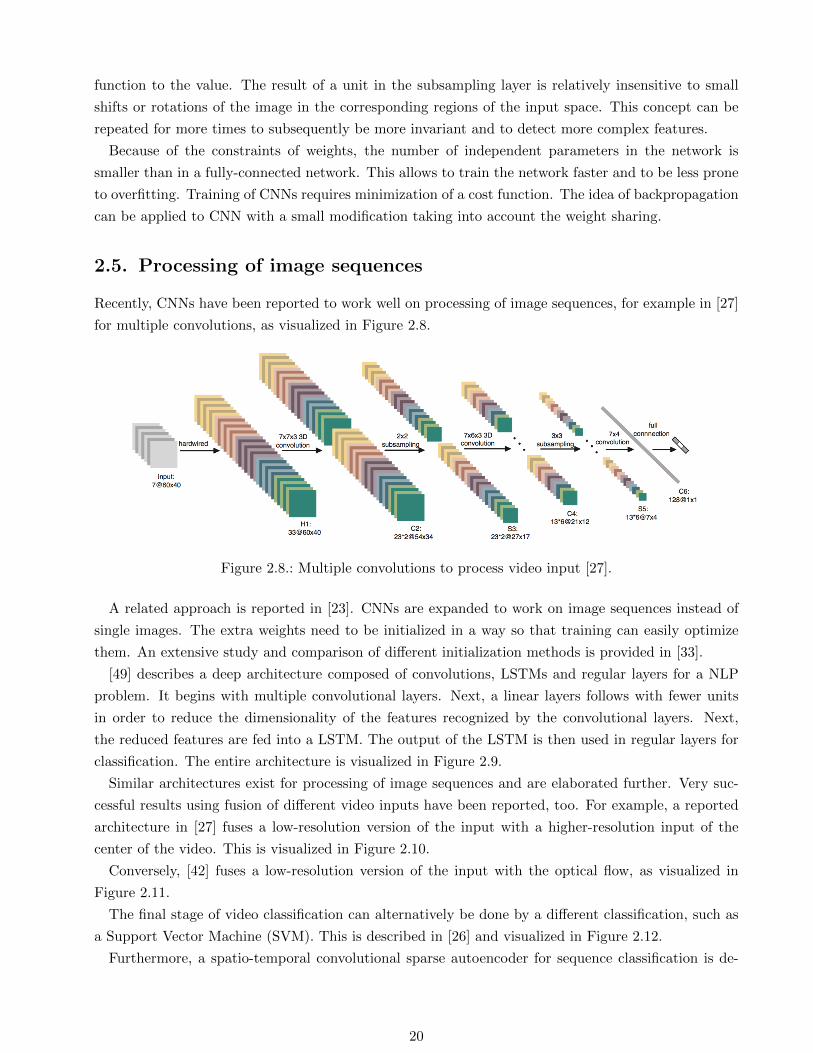
Recently, CNNs have been reported to work well on processing of image sequences, for example in [27]
for multiple convolutions, as visualized in Figure 2.8.
Figure 2.8.: Multiple convolutions to process video input [27].
A related approach is reported in [23]. CNNs are expanded to work on image sequences instead of
single images. The extra weights need to be initialized in a way so that training can easily optimize
them. An extensive study and comparison of different initialization methods is provided in [33].
[49] describes a deep architecture composed of convolutions, LSTMs and regular layers for a NLP
problem. It begins with multiple convolutional layers. Next, a linear layers follows with fewer units
in order to reduce the dimensionality of the features recognized by the convolutional layers. Next,
the reduced features are fed into a LSTM. The output of the LSTM is then used in regular layers for
classification. The entire architecture is visualized in Figure 2.9.
Similar architectures exist for processing of image sequences and are elaborated further. Very suc-
cessful results using fusion of different video inputs have been reported, too. For example, a reported
architecture in [27] fuses a low-resolution version of the input with a higher-resolution input of the
center of the video. This is visualized in Figure 2.10.
Conversely, [42] fuses a low-resolution version of the input with the optical flow, as visualized in
Figure 2.11.
The final stage of video classification can alternatively be done by a different classification, such as
a Support Vector Machine (SVM). This is described in [26] and visualized in Figure 2.12.
Furthermore, a spatio-temporal convolutional sparse autoencoder for sequence classification is de-
20
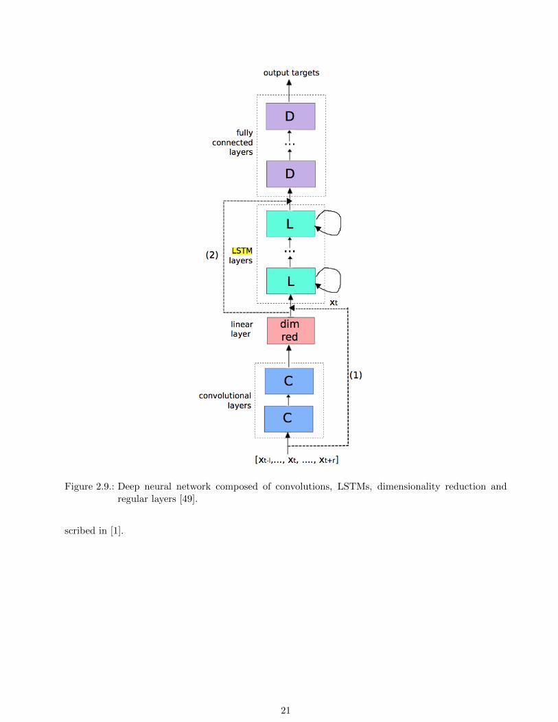
Figure 2.9.: Deep neural network composed of convolutions, LSTMs, dimensionality reduction andregular layers [49].
scribed in [1].
21
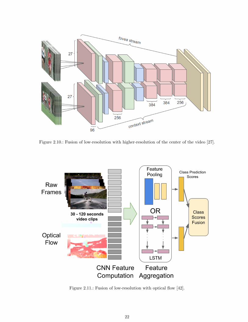
Figure 2.10.: Fusion of low-resolution with higher-resolution of the center of the video [27].
Figure 2.11.: Fusion of low-resolution with optical flow [42].
22
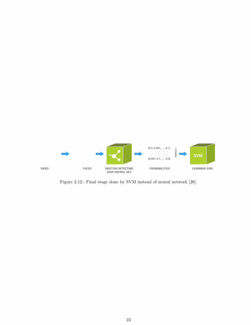
Figure 2.12.: Final stage done by SVM instead of neural network [26].
23

3. Selection of databases
In this chapter, various popular databases relevant to action unit recognition are presented. Each
database includes annotations per frame of the respective action units, among other features. Further-
more, statistics of the distribution of action units were generated for each database in order to select
databases rich of smiles.
3.1. FACS coding
The Facial Action Coding System (FACS) is a system to taxonomize any facial expression of a human
being by their appearance on the face. It was published by Paul Ekman and Wallace V. Friesen in 1978
[6]. Relevant to this thesis are so-called Action Units (AUs), which are the basic actions of individual
facial muscles or groups of muscles. Action units are either set or unset. If set, different levels of
intensity are possible.
3.2. Available databases
Popular databases in the field of action unit recognition and studies of facial expressions include the
following, which are presented briefly in this section. The reader is referred to the relevant literature
for details.
The Affectiva-MIT Facial Expression Dataset (AMFED) [36] contains 242 facial videos (168,359
frames), which were recorded in the wild (real world conditions). The Chinese Academy of Sciences
Micro-expression (CASME) [58] database was filmed at 60fps and contains 195 micro-expressions of
22 male and 13 female participants. The Denver Intensity of Spontaneous Facial Action (DISFA)
[35] database contains videos of 15 male and 12 female subjects of different ethnicities. Action unit
annotations are on different levels of intensity. The Geneva Multimodal Emotion Portrayals (GEMEP)
[2] contains audio and video recordings of 10 actors which portray 18 affective states. The MAHNOB
Laughter [47] database contains 22 subjects recorded using a video camera, a thermal camera and
two microphones. Recorded were laughter, posed smiles, posed laughter and speech. It includes 180
sessions with a total duration of 3h and 49min.
The UNBC-McMaster Shoulder Pain Expression Archive Database [32] contains 200 video sequences
of participants that were suffering from shoulder pain and their corresponding spontaneous facial
expressions. In total, it includes 48,398 FACS coded frames.
24
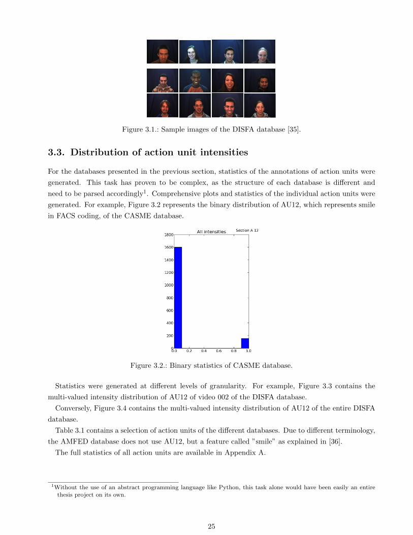
Figure 3.1.: Sample images of the DISFA database [35].
3.3. Distribution of action unit intensities
For the databases presented in the previous section, statistics of the annotations of action units were
generated. This task has proven to be complex, as the structure of each database is different and
need to be parsed accordingly1. Comprehensive plots and statistics of the individual action units were
generated. For example, Figure 3.2 represents the binary distribution of AU12, which represents smile
in FACS coding, of the CASME database.
Figure 3.2.: Binary statistics of CASME database.
Statistics were generated at different levels of granularity. For example, Figure 3.3 contains the
multi-valued intensity distribution of AU12 of video 002 of the DISFA database.
Conversely, Figure 3.4 contains the multi-valued intensity distribution of AU12 of the entire DISFA
database.
Table 3.1 contains a selection of action units of the different databases. Due to different terminology,
the AMFED database does not use AU12, but a feature called ”smile” as explained in [36].
The full statistics of all action units are available in Appendix A.
1Without the use of an abstract programming language like Python, this task alone would have been easily an entirethesis project on its own.
25
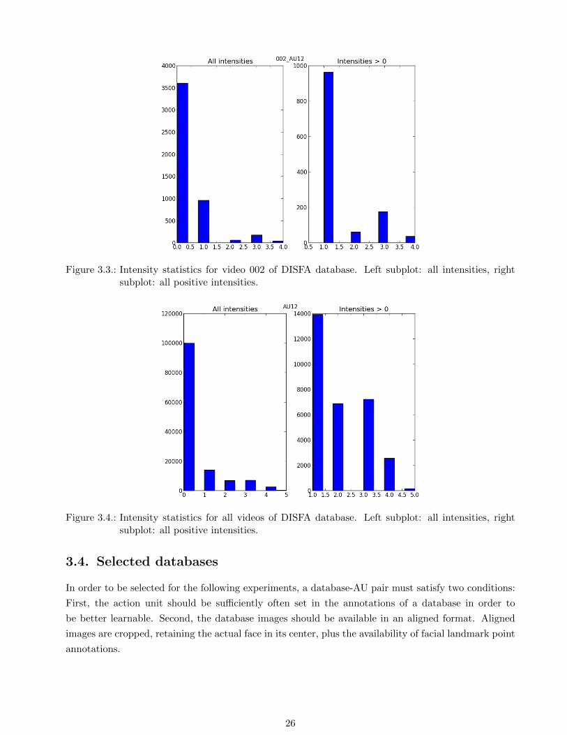
Figure 3.3.: Intensity statistics for video 002 of DISFA database. Left subplot: all intensities, rightsubplot: all positive intensities.
Figure 3.4.: Intensity statistics for all videos of DISFA database. Left subplot: all intensities, rightsubplot: all positive intensities.
3.4. Selected databases
In order to be selected for the following experiments, a database-AU pair must satisfy two conditions:
First, the action unit should be sufficiently often set in the annotations of a database in order to
be better learnable. Second, the database images should be available in an aligned format. Aligned
images are cropped, retaining the actual face in its center, plus the availability of facial landmark point
annotations.
26
AMFED CASME DISFA GEMEP MAHNOB Laughter Shoulder Pain
AU1 - 1976 8778 1584 - -
AU12 - 264 30794 2692 - 6887
AU16 - 126 - 310 - -
AU21 - - - 95 - -
Laughter - - - - 6404 -
Smile 77062 - - - - -
negAU12 350 - - - - -
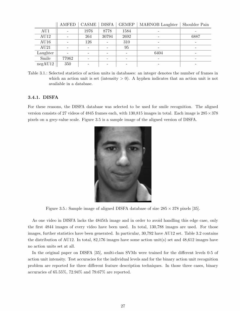
Table 3.1.: Selected statistics of action units in databases: an integer denotes the number of frames inwhich an action unit is set (intensity > 0). A hyphen indicates that an action unit is notavailable in a database.
3.4.1. DISFA
For these reasons, the DISFA database was selected to be used for smile recognition. The aligned
version consists of 27 videos of 4845 frames each, with 130,815 images in total. Each image is 285×378
pixels on a grey-value scale. Figure 3.5 is a sample image of the aligned version of DISFA.
Figure 3.5.: Sample image of aligned DISFA database of size 285× 378 pixels [35].
As one video in DISFA lacks the 4845th image and in order to avoid handling this edge case, only
the first 4844 images of every video have been used. In total, 130,788 images are used. For those
images, further statistics have been generated. In particular, 30,792 have AU12 set. Table 3.2 contains
the distribution of AU12. In total, 82,176 images have some action unit(s) set and 48,612 images have
no action units set at all.
In the original paper on DISFA [35], multi-class SVMs were trained for the different levels 0-5 of
action unit intensity. Test accuracies for the individual levels and for the binary action unit recognition
problem are reported for three different feature description techniques. In those three cases, binary
accuracies of 65.55%, 72.94% and 79.67% are reported.
27

Intensity Count
0 999961 139422 68683 72334 25775 172
Table 3.2.: Distribution of AU12 in DISFA.
3.4.2. Others
For the same reasons, the shoulder pain database is of further interest of smile detection for further
experiments, such as a multi-database smile detector. Furthermore, the laughter in the MAHNOB
Laughter database may be of interest in future experiments, as laughter includes smile. AMFED was
not considered further, as ”smile” is not AU12, but something slightly different, but may be of interest
in further experiments, too.
28
4. Model
The goal of this project is to recognize and predict action units from videos, in particular smiles. A
regular deep neural network would not suit this task for two main reasons: First, deep neural networks
do not support handling translation or other distortions of the input, which happen frequently in facial
videos. Second, deep feed-forward neural networks do not have a state, therefore making processing
of videos difficult as they require handling of states in order to recognize or predict action units. In
this chapter, the proposed model for smile detection is explained in detail, of which the first part is
implemented. In order to train it in a reasonable amount of time, a powerful underlying computing
infrastructure has been used.
4.1. Proposed model
Based on findings described in Chapter 2.5, an initial model has been defined and refined after discus-
sions with other experts, including Sinisa Todorovic [57]. The model can be summarized as follows:
Feature extraction in the first stage, followed by the temporal part.
For feature extraction, a CNN is trained on images of the entire face or an area suitable for smile
detection, such as the mouth. This CNN is followed by one or multiple layers of a regular (dense)
neural network for discrimination of the features. The exact architecture of the network, such as
the number of convolutions, number of hidden layers, etc. is subject to model selection, which was
extensively performed in Chapter 5. The size of the input is also subject to model selection as one
input unit is needed per input pixel. The larger the input image, the better, as more data and details
are available. Conversely, the model becomes more complex and more difficult to train, with overfitting
or long training time as possible consequences.
The output of this network is fed into the second part, which handles temporal relationships. There
are different possibilities how to model it. On the one hand, state-of-the-art methods, such as Hidden
Markov Models (HMMs), could be used. On the other hand, recurrent neural networks are of particular
interest for this project. As described in Chapter 2.3, LSTMs are reported to perform well on temporal
data and are known to be able to outperform HMMs. Therefore, LSTMs are chosen for this part,
followed by one or multiple layers of a regular neural network for discrimination of the features.
The proposed model is visualized in Figure 4.1.
In the literature, related experiments on other databases have been performed. Results were repor-
ted, in which the two parts were subsequently trained, i.e. the feature extraction was trained first and
used to train the temporal part [42] [48]. In contrast, other models that were trained end-to-end are
described in the literature, too [48] [15] [17]. An end-to-end trained model seems preferable for those
experiments and would therefore also be interesting to investigate.
29
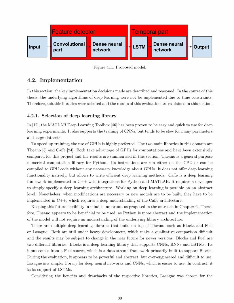
Figure 4.1.: Proposed model.
4.2. Implementation
In this section, the key implementation decisions made are described and reasoned. In the course of this
thesis, the underlying algorithms of deep learning were not be implemented due to time constraints.
Therefore, suitable libraries were selected and the results of this evaluation are explained in this section.
4.2.1. Selection of deep learning library
In [12], the MATLAB Deep Learning Toolbox [46] has been proven to be easy and quick to use for deep
learning experiments. It also supports the training of CNNs, but tends to be slow for many parameters
and large datasets.
To speed up training, the use of GPUs is highly preferred. The two main libraries in this domain are
Theano [3] and Caffe [24]. Both take advantage of GPUs for computations and have been extensively
compared for this project and the results are summarized in this section. Theano is a general purpose
numerical computation library for Python. Its instructions are run either on the CPU or can be
compiled to GPU code without any necessary knowledge about GPUs. It does not offer deep learning
functionality natively, but allows to write efficient deep learning methods. Caffe is a deep learning
framework implemented in C++ with integrations for Python and MATLAB. It requires a developer
to simply specify a deep learning architecture. Working on deep learning is possible on an abstract
level. Nonetheless, when modifications are necessary or new models are to be built, they have to be
implemented in C++, which requires a deep understanding of the Caffe architecture.
Keeping this future flexibility in mind is important as proposed in the outreach in Chapter 6. There-
fore, Theano appears to be beneficial to be used, as Python is more abstract and the implementation
of the model will not require an understanding of the underlying library architecture.
There are multiple deep learning libraries that build on top of Theano, such as Blocks and Fuel
or Lasagne. Both are still under heavy development, which make a qualitative comparison difficult
and the results may be subject to change in the near future for newer versions. Blocks and Fuel are
two different libraries. Blocks is a deep learning library that supports CNNs, RNNs and LSTMs. Its
input comes from a Fuel source, which is a data stream framework primarily built to support Blocks.
During the evaluation, it appears to be powerful and abstract, but over-engineered and difficult to use.
Lasagne is a simpler library for deep neural networks and CNNs, which is easier to use. In contrast, it
lacks support of LSTMs.
Considering the benefits and drawbacks of the respective libraries, Lasagne was chosen for the
30
implementation of the model. As Lasagne lacks support of LSTMs, a separate LSTM library was
chosen, as described in the following section.
4.2.2. Selection of LSTM library
There is an extension of Lasagne for LSTMs [11] which prove to be effective in the evaluation. It is
most straightforward to use together with the feature detector of the first stage. Also, an end-to-end
training of the entire model is possible using this library. Nonetheless, the project has only one main
committer coming with uncertainty if it will be kept in sync with Lasagne in the future.
Support for use of GPUs for training is also offered by CURRENNT [50], a C++ library for recurrent
neural networks. No support for Python is offered by this library, making integration into existing
code of the feature detector more difficult.
Furthermore, RNNLIB [51] is a popular library for recurrent neural networks, including LSTMs. Its
Python wrapper allows easy integration in existing code of the feature detector. It lacks support of
GPUs, which may come with long training time for the large database of this project.
Based on these considerations, the Lasagne LSTM extension seems most preferable because of the
same data format, functions and easy integration into existing code.
4.2.3. Progress of implementation
As mentioned previously, Lasagne is still under development, which proved to make the implementation
of the model more time consuming than initially expected due to changes in the API. In particular,
a lot of demo code did not work correctly, leaving the author of this thesis with unexpected behavior
and no useful error messages.
Once these issues were sorted out, the implementation of the training and model selection of the
feature detector in Chapter 5 was straightforward due to the abstraction provided by Lasagne.
In the course of this project, only the first stage of the model, the feature detector, was implemented.
Due to time constraints, the second part could not be implemented. Because of the overall high test
accuracies of the feature detector in Chapter 5, there is also a lesser need of adding temporal capabilities
to this model at this point.
4.3. Computing infrastructure
In initial experiments, GPU acceleration provided by Theano has proven to speed up the training by
factor 3-10 in comparison to a CPU. The experiments of this project cannot be run on the GPU of a
modern notebook, such as a latest MacBook Pro, because the provided RAM of the GPU is too small
to fit some of the models. In these experiments, various GPUs were used including a GeForce GTX
TITAN Black [10] or a even more powerful Tesla K40c [45]. For the Tesla series, significant speedups
have been measured for different applications as collected in Figure 4.2.
For the experiments in Chapter 5, a server containing a Tesla K40c with 12 GB of GPU RAM and 64
GB of regular RAM was chosen. Both memories are sufficiently large to store the model and training
data. The Tesla would allow to run multiple experiments at the same time, as a single experiment
only uses a fraction of the GPU RAM as visualized in Figure 4.3.
31
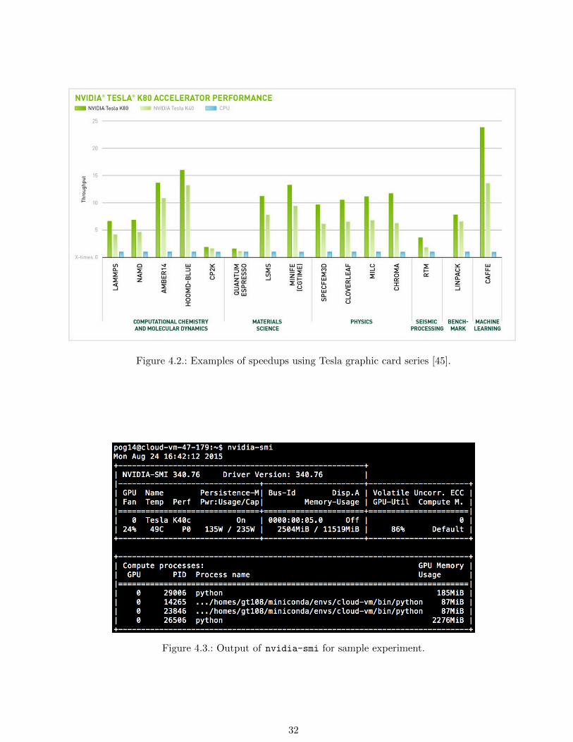
Figure 4.2.: Examples of speedups using Tesla graphic card series [45].
Figure 4.3.: Output of nvidia-smi for sample experiment.
32
5. Towards a static convolutional smile
detector
In this chapter, experiments for smile detection using the convolutional feature detector are performed
on the DISFA database. An essential task is model selection to pick the best architecture from a
large permutation of many possible parameters. Starting with regular smile detection, only low or
high intensity smiles are retained for smile recognition. Finally, low intensity smiles are discriminated
against high intensity smiles. In order to perform the experiments in time, preliminary assumptions
made are reasoned.
5.1. Selected parameters and assumptions
Today, there is a lack of literature or research on neural networks for sample complexity or general rules
to choose an architecture. Therefore, in order to find good parameter values for the feature detector,
model selection needs to be performed.
5.1.1. Candidate parameters to be optimized
There are many possible parameters to be optimized and reported in the literature, including:
1. Number of convolution-pooling pairs
2. Architecture of convolutions, such as the number of feature maps and their size
3. Architecture of poolings, such as the type of pooling, pooling size or whether to pool at all
4. Type of activation function, such as rectified linear units (ReLU), softmax or Sigmoid
5. Type of regularization, such as dropout or L2
6. Number of hidden layers
7. Number of units in the hidden layers
8. Learning rate
9. Momemtum
Parameters 1 to 3 concern the convolutional part of the network. A number of optimizations are
possible, such as the number of convolution-pooling pairs and how to build the individual convolutions
and poolings. The parameters to be optimized include the size and number of feature maps, the type
33
of pooling and the pooling size. Another question is whether to use pooling at all, as good results
without pooling were reported in [52].
Activation functions are described in Chapter 2.2.2 and the remaining parameters are described in
[12]. A further discussion is omitted in this part of this thesis.
5.1.2. Selected parameters and values
In order to reduce the duration of the model selection to a realistic scale, various assumptions were
made. For convolutions and subsequent poolings, many parameters could be optimized in model
selection, exploding the possible search space. Therefore, a number of parameters are fixed, based on
experiments with the same library on MNIST: convolutions are for areas of 5 × 5 pixels and in each
convolutional layer, 32 feature maps are used. Subsequent pooling is for areas of 2× 2 pixels and only
max pooling is used, as the concrete type of pooling is reported to be less relevant in the literature [42].
Convolution-pooling pairs are used throughout the experiments, no single convolutions not followed
by pooling [52] [49]. For reasons of simplicity, a convolution-pooling pair is simply named convolution
in the remainder of this thesis.
The benefits of rectified linear (ReLU) units are discussed in Chapter 2.2.2. As they are reported
to outperform Sigmoid units, ReLU units are used throughout all experiments. As the only exception,
softmax is used in the output layer.
For regularization, dropout is the only explicit regularization method used in the model selection.
L2 regularization is not used at all, as a wide spectrum of possible values would have to be tested. As
a consequence, model selection would take significantly more time. Furthermore, ReLU units serve as
an implicit regularization method because they lead to sparse activations in the network.
The learning rate is fixed to α = 0.01 and not subject to model selection as it would also significantly
prolong the model selection. The same considerations apply to the momentum, which is fixed to
µ = 0.9. Overall, the momentum is expected to have less impact due to the use of ReLU units, as
reasoned in Chapter 2.2.2. Both values are taken from the Lasagne MNIST showcase, for which they
worked effectively.
Based on these considerations, the following parameters are subject to model selection: number of
convolution-pooling pairs, number of hidden layers, number of units in hidden layers and and dropout.
Table 5.1 contains the values chosen for model selection of the respective parameters and default
values. The values and default values were picked, based on prior experience and initial assumptions.
For the default values, the simplest values were picked, except for dropout. For dropout, p = 0.5 is
chosen in the Lasagne MNIST showcase and proved to be effective in initial bottom line experiments
in Chapter 5.2. The table also contains in parentheses the short name chosen for parameters, which
are used in subsequent tables.
34

Parameter Values Default value
Number of convolution-pooling pairs (#Convs) 1, 2, 3 1
Number of hidden layers (#Hidden layers) 1, 2, 3 1
Number of units in hidden layers (#Units hidden layers) 100, 200, 300, 400 100
Dropout 0, 0.1, 0.5, 0.7 0.5
Table 5.1.: Parameters and possible values used in model selection.
5.1.3. Cost function and performance metrics
For the following model selection, the cross-entropy loss/cost function is used for m examples, hypo-
thesis hθ and target values y(i):
J(θ) =1
m
m∑i=1
(−y(i) log(hθ(x
(i)))− (1− y(i)) log(1− hθ(x(i))))
(5.1)
In contrast to other possible cost functions, such as least squares, it is known to generalize better and
that training has been reported to converge faster [40].
In the following model selection, both the cross-entropy loss and the test accuracy (classification rate
for this binary problem) are output. This decision has been made because of the following reasons:
the cross-entropy loss is mathematically more accurate, whereas the test accuracy is more intuitive for
humans. Nonetheless, it must be noted that both metrics are different and not fully comparable.
5.1.4. Input size
All experiments are run for two different sources of data: mouth or entire face in order to find out if
the mouth alone is as meaningful as the face for smile detection, see Figure 5.1.
(a) Mouth input (b) Face input
Figure 5.1.: Different input parts: a) mouth, b) face [35]. (Not at actual input size/proportions.)
The aligned images are 285× 378 pixels, as covered in Chapter 3.4.1.
35
Because of facial landmarks contained in the aligned images, the location of the mouth can be
computed. A bounding box to include the mouth of every image was computed. This bounding box
is of size 128 × 104 pixels, which would be 13,312 input units. In order to reduce overfitting and to
speed up training, both dimensions have been reduced to 2/3 of their original size using a bilinear
interpolation. Therefore, the mouth input is 85× 69 pixels, requiring 5,865 input units in total.
The same considerations have been applied to the input of the entire face. The size reduction factor
is stronger than for the mouth in order to do the training in a realistic time, at the expense of possibly
meaningful features. As a result, faces are fed in as 95 × 121 pixels, requiring 11,495 input units in
total.
MNIST [30] is a commonly used toy problem in many deep learning publications. MNIST consists
of 60,000 test examples of size 28 × 28 pixels. Therefore, this training task is not only more complex
in terms of what to detect, but also in terms of the amount of data points and number of input pixels.
5.2. Bottom lines
In order to evaluate the underlying software and hardware infrastructure, very initial experiments on
much smaller inputs have been performed on fixed architectures. Mouth images are of size 37 × 28,
whereas face images are of size 40 × 48. The architectures used are a regular neural network of 2
hidden layers of 800 units each, followed by a softmax output layer of 2 units. The other architecture
is a convolutional neural network of two convolution and pooling stages and a fully connected hidden
layer in front of the softmax output layer. Details are omitted for these initial experiments. The test
losses and accuracies are summarized in Table 5.2.
Input Network Test loss Test accuracy
Mouth NN 0.258068 90.16%
Mouth CNN 0.167116 93.34%
Face NN 0.331730 86.92%
Face CNN 0.188780 92.36%
Table 5.2.: Bottom line experiments for both inputs for NN and CNN. Optimal values per input inbold.
For both inputs, the CNNs outperform the NNs by a margin of 3.18% and 5.44% for mouth and
face, respectively. Both CNNs achieve an accuracy of over 90%. Nonetheless, the NNs perform well
given the noise in the the data. The CNN for the input of the mouth outperforms the CNN for the
input of the face. This cannot be generalized as the face images are too small for practical purposes
and because no model selection was performed. Nonetheless, these initial results serve as a bottom
line for future experiments.
5.3. Model selection for full dataset
For the following model selection, the entire DISFA database was split in a training/validation/test
ratio of 60%/20%/20%. The validation set was used exclusively at each epoch for loss validation.
36
After the respective number of epochs, the test set was used to compute test loss and test accuracy.
Each of the parameters was optimized independently using default values of the other parameters at
the same time. Model selection was performed for two different types of input: mouth or the entire
face and for two different number of epochs: 10 and 50 epochs. An exhaustive search or more epochs
were not possible due to the enormous training times, for which statistics of each trained permutation
are available in Appendix B. In most examples, the validation loss drops off quickly before converging
slowly, as visualized in Figure 5.2. Therefore, at this stage of the experiment, the maximum number of
epochs is set to 50. Each experiment is performed exactly once, which comes with a certain bias, but
reduces training time significantly. Chapter 5.5 provides an experimental justification that this bias is
low.
Figure 5.2.: Change of validation loss for mouth data for 2 convolutional layers, other parametersdefault. For full dataset.
5.3.1. Mouth
For the mouth input, Tables C.1 and C.2 contain the result of the model selection for 10 and 50 epochs,
respectively. The first line of each table is the combination of all default values and therefore serve as
a bottom line in each experiment. For 10 epochs, for none of the four parameters the default one was
chosen to be better than the ones available in the selection. In particular, lowest losses are returned
for 2 convolutions, 3 hidden layers, 400 hidden units per layer and a dropout value of 0.1. Overall, test
accuracies are on a high level and individually tested values for the parameters have minor effect as
test accuracies range from 90.99% to 94.54%. A dropout value of 0.1 results in the highest accuracy,
whereas a dropout value of 0.7 reduces the test accuracy the most.
For 50 epochs, these selected values remain the same, except that in this case 2 hidden layers have
the lowest test loss. Overall, test accuracies are on a even higher level and individually tested values
37
for the parameters have minor effect as test accuracies range from 94.54% to 97.70%. A dropout value
of 0.1 results in the highest accuracy, whereas a dropout value of 0 reduces the test accuracy the most.
5.3.2. Face
Conversely, for the entire face input, Tables C.3 and C.4 contain the result of the model selection for
10 and 50 epochs, respectively. For 10 epochs, the default one was chosen to be better than the ones
available in the selection for the number of convolutions and the number of hidden units. In particular,
lowest losses are returned for 1 convolution, 2 hidden layers, 100 hidden units per layer and a dropout
value of 0. Overall, test accuracies are on a high level and individually tested values for the parameters
have minor effect as test accuracies range from 94.69% to 96.36%. A dropout value of 0 results in the
highest accuracy, whereas 3 convolutions reduce the test accuracy the most.
For 50 epochs, these selected values remain the same for the number of convolutions and dropout.
The optimal number of hidden layers and hidden units change to 1 and 400, respectively. Overall,
test accuracies are on a even higher level and individually tested values for the parameters have minor
effect as test accuracies range from 97.37% to 98.57%. A dropout value of 0 results in the highest
accuracy, whereas a dropout value of 0.7 reduces the test accuracy the most.
5.3.3. Comparison of mouth vs. face
For both input parts, mouth and face, the model selection for 50 epochs returned different optimal
parameters, which are collected in Table 5.3.
Input #Convs #Hidden layers #Units hidden layers Dropout
Mouth 2 2 400 0.1
Face 1 1 400 0
Table 5.3.: Selected parameter values for mouth and face input. For full dataset.
Overall, the test accuracies are slightly higher for the input of the entire face than just the mouth
for 10 and 50 epochs. Precisely, the test accuracy is about 3% higher for the entire face for 10 epochs.
This is logical, as smile is not only visible on the mouth of humans, but also in other area, such as the
cheeks. This margin reduces to about 2% for 50 epochs.
Training time for the entire face is about 20% higher for the entire face than for just the mouth.
This is surprisingly less than expected since the number of input pixels is nearly double than for the
mouth.
5.4. Model selection for reduced dataset
In the model selection in Chapter 5.3, the entire DISFA database was used. As measured in Chapter 3.4.1,
48,612 of the entire 130,788 images are neutral, meaning no action units are set. The more neutral
images, the easier the training of the smile detector. Therefore, in this section, a reduced set of DISFA
is used. It consists of all 82,176 images that have some action unit(s) sets and 30% of the 48,612
remaining neutral images, making 96,759 images in total.
38
The setup of the experiments remains the same, in particular the ratio of training/validation/test
examples, the two different input times, mouth and face, the number of epochs and the non-exhaustive
model selection. Training time statistics of each trained permutation are available in Appendix B.
5.4.1. Mouth
For the mouth input, Tables C.5 and C.6 contain the result of the model selection for 10 and 50 epochs,
respectively. For 10 epochs, for none of the four parameters the default one was chosen to be better
than the ones available in the selection. In particular, lowest losses are returned for 2 convolutions, 2
hidden layers, 400 hidden units per layer and a dropout value of 0. Overall, test accuracies are on a
high level and individually tested values for the parameters have minor effect as test accuracies range
from 89.46% to 93.62%. 2 convolutions result in the highest accuracy, whereas a dropout value of 0.7
reduces the test accuracy the most.
For 50 epochs, these selected values remain the same, except that in this case 300 hidden units have
the lowest test loss. Overall, test accuracies are on a even higher level and individually tested values
for the parameters have minor effect as test accuracies range from 95.84% to 97.59%. A dropout value
of 0 results in the highest accuracy, whereas all default values combined reduces the test accuracy the
most.
5.4.2. Face
Conversely, for the entire face input, Tables C.7 and C.8 contain the result of the model selection for
10 and 50 epochs, respectively. For 10 epochs, the default one was chosen to be better than the ones
available in the selection for the number of convolutions. In particular, lowest losses are returned for
1 convolution, 2 hidden layers, 300 hidden units per layer and a dropout value of 0. Overall, test
accuracies are on a high level and individually tested values for the parameters have minor effect as
test accuracies range from 92.65% to 95.44%. A dropout value of 0 results in the highest accuracy,
whereas 3 convolutions reduce the test accuracy the most.
For 50 epochs, these selected values remain the same for the number of convolutions and number
of hidden units. The optimal number of hidden layers and dropout change to 1 and 0.1, respectively.
Overall, test accuracies are on a even higher level and individually tested values for the parameters
have minor effect as test accuracies range from 95.91% to 98.16%. A dropout value of 0.1 results in
the highest accuracy, whereas 3 hidden layers reduce the test accuracy the most.
5.4.3. Comparison of mouth vs. face
For both input parts, mouth and face, the model selection for 50 epochs returned different optimal
parameters, which are collected in Table 5.4.
Input #Convs #Hidden layers #Units hidden layers Dropout
Mouth 2 2 300 0
Face 1 1 300 0.1
Table 5.4.: Selected parameter values for mouth and face input. For reduced dataset.
39
Overall, the test accuracies are slightly higher for the input of the entire face than just the mouth
for 10 and 50 epochs. Precisely, the test accuracy is about 2% higher for the entire face for 10 epochs.
This margin reduces to about 1% for 50 epochs.
Training time for the entire face is also about 20% higher for the entire face than for just the mouth.
5.5. Repeatability of experiments
Each experiment was performed exactly once. Training of neural networks is subject to a random
initialization of the weights at the beginning of the training and to the random split of the data into
training, validation and test sets. Therefore, repeating an experiment may return different results. If
this difference is large, each experiment must be conducted for multiple times to use its median in
the model selection decisions. In order to assess if such a time-consuming process is necessary or not,
the training of the neural network for 2 hidden layers for the mouth input in the model selection was
conducted 10 times for the full dataset. The results are available in Table 5.5 with standard deviation
of 0.041725% in the test accuracy. Because of this low standard deviation, performing each experiment
exactly once has only a very low bias and is therefore relatively safe to do for reasons of faster training
time. The standard deviation of the cross-entropy loss has been omitted as it is not meaningful to
humans.
Experiment number Test accuracy
1 97.58%
2 97.51%
3 97.59%
4 97.49%
5 97.55%
6 97.62%
7 97.59%
8 97.57%
9 97.52%
10 97.61%
Standard deviation 0.041725%
Table 5.5.: Repeatability of training of architecture with default values and 2 hidden layers for mouthfor 50 epochs: standard deviation of test accuracies. Optimal values in bold. For fulldataset.
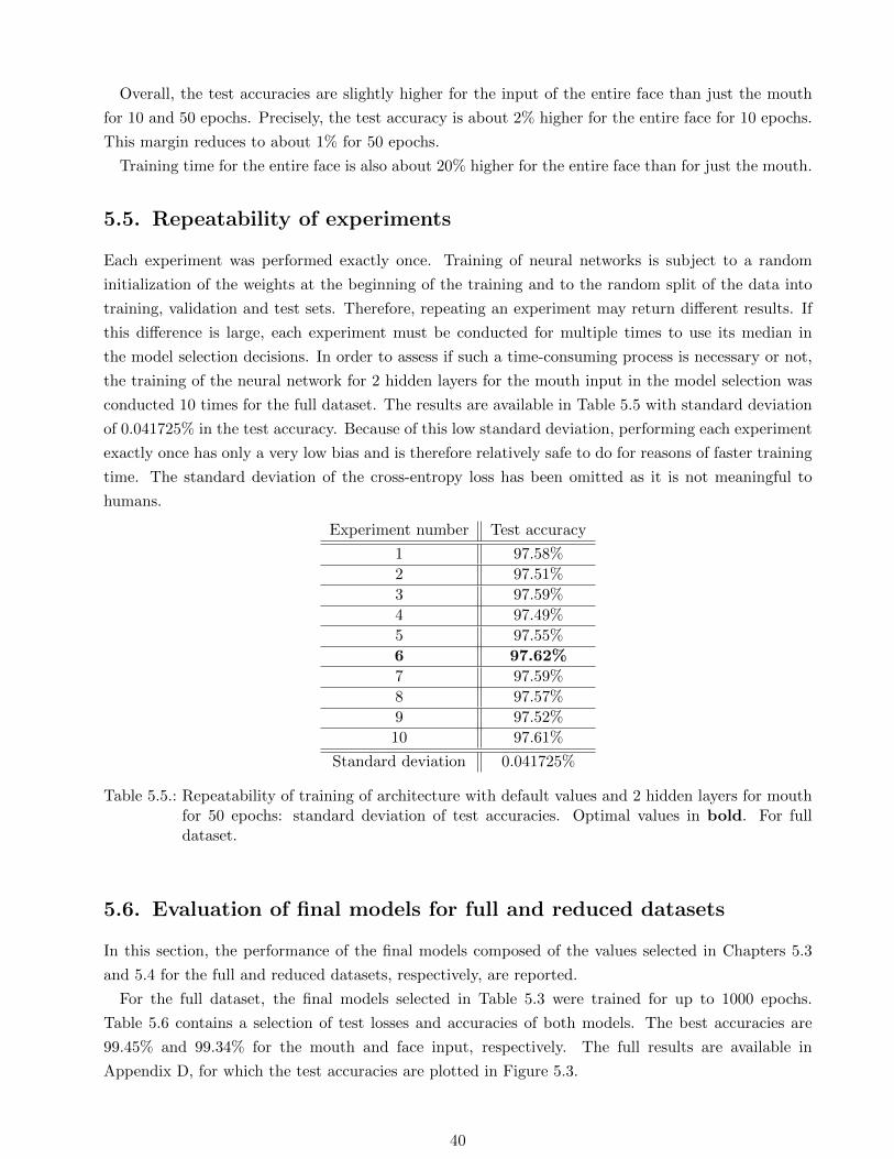
5.6. Evaluation of final models for full and reduced datasets
In this section, the performance of the final models composed of the values selected in Chapters 5.3
and 5.4 for the full and reduced datasets, respectively, are reported.
For the full dataset, the final models selected in Table 5.3 were trained for up to 1000 epochs.
Table 5.6 contains a selection of test losses and accuracies of both models. The best accuracies are
99.45% and 99.34% for the mouth and face input, respectively. The full results are available in
Appendix D, for which the test accuracies are plotted in Figure 5.3.
40
Mouth Face#Epochs Test loss Test accuracy Test loss Test accuracy
10 0.114402 95.75% 0.094356 96.46%
100 0.027658 99.08% 0.030599 99.01%
200 0.025298 99.28% 0.027087 99.22%
700 0.033508 99.45% 0.039649 99.31%
1000 0.038099 99.43% 0.044800 99.34%
Table 5.6.: Result of model selection for mouth and face with the combined parameters for selectedepochs. Optimal values per part in bold. For full dataset.
Figure 5.3.: Change of test accuracy for mouth and face data over 1000 epochs. For full dataset.
For both inputs, the training is near to the best results after 200 epochs, after which the training
wanders around the maximum. For the mouth and face input, the best accuracies are achieved after
700 and 1000 epochs, respectively. For the test loss however, the minima are achieved after 200 epochs.
This is a case in which accuracy and cross-entropy are not fully comparable.
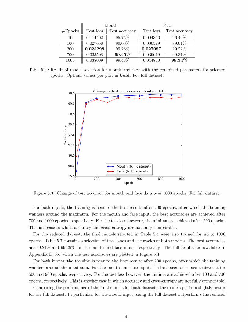
For the reduced dataset, the final models selected in Table 5.4 were also trained for up to 1000
epochs. Table 5.7 contains a selection of test losses and accuracies of both models. The best accuracies
are 99.24% and 99.26% for the mouth and face input, respectively. The full results are available in
Appendix D, for which the test accuracies are plotted in Figure 5.4.
For both inputs, the training is near to the best results after 200 epochs, after which the training
wanders around the maximum. For the mouth and face input, the best accuracies are achieved after
500 and 900 epochs, respectively. For the test loss however, the minima are achieved after 100 and 700
epochs, respectively. This is another case in which accuracy and cross-entropy are not fully comparable.
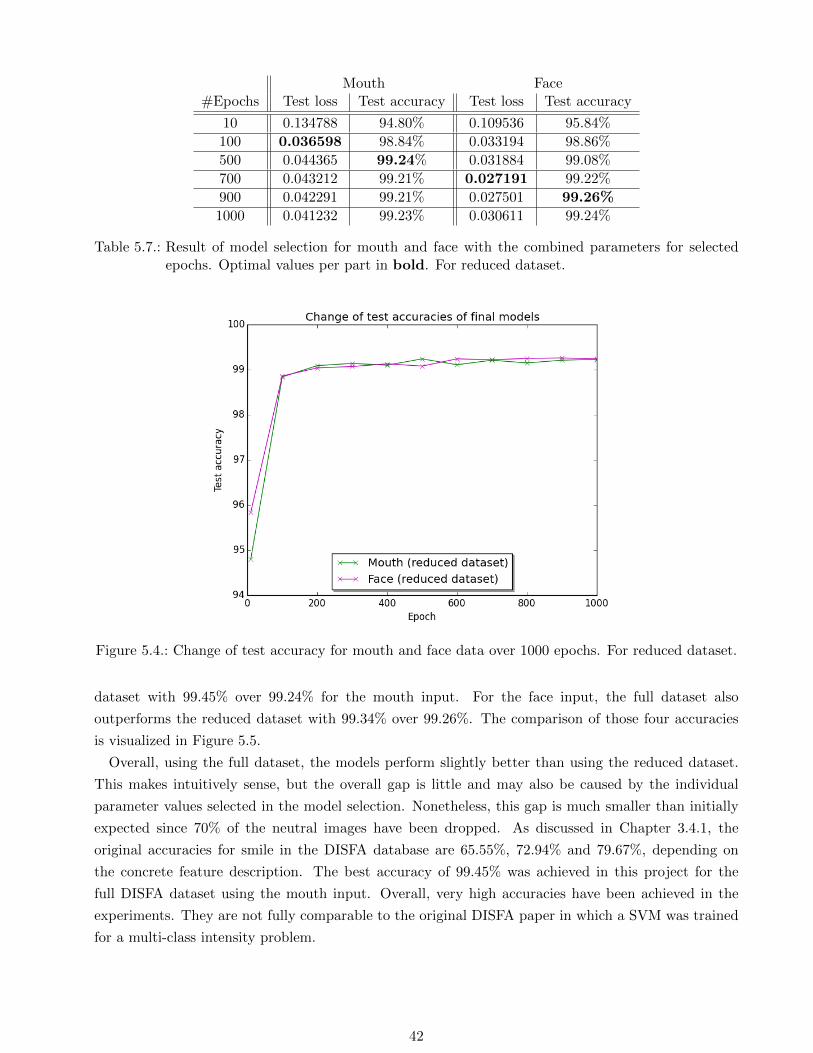
Comparing the performance of the final models for both datasets, the models perform slightly better
for the full dataset. In particular, for the mouth input, using the full dataset outperforms the reduced
41
Mouth Face#Epochs Test loss Test accuracy Test loss Test accuracy
10 0.134788 94.80% 0.109536 95.84%
100 0.036598 98.84% 0.033194 98.86%
500 0.044365 99.24% 0.031884 99.08%
700 0.043212 99.21% 0.027191 99.22%
900 0.042291 99.21% 0.027501 99.26%
1000 0.041232 99.23% 0.030611 99.24%
Table 5.7.: Result of model selection for mouth and face with the combined parameters for selectedepochs. Optimal values per part in bold. For reduced dataset.
Figure 5.4.: Change of test accuracy for mouth and face data over 1000 epochs. For reduced dataset.
dataset with 99.45% over 99.24% for the mouth input. For the face input, the full dataset also
outperforms the reduced dataset with 99.34% over 99.26%. The comparison of those four accuracies
is visualized in Figure 5.5.
Overall, using the full dataset, the models perform slightly better than using the reduced dataset.
This makes intuitively sense, but the overall gap is little and may also be caused by the individual
parameter values selected in the model selection. Nonetheless, this gap is much smaller than initially
expected since 70% of the neutral images have been dropped. As discussed in Chapter 3.4.1, the
original accuracies for smile in the DISFA database are 65.55%, 72.94% and 79.67%, depending on
the concrete feature description. The best accuracy of 99.45% was achieved in this project for the
full DISFA dataset using the mouth input. Overall, very high accuracies have been achieved in the
experiments. They are not fully comparable to the original DISFA paper in which a SVM was trained
for a multi-class intensity problem.
42
Figure 5.5.: Change of test accuracy for mouth and face data over 1000 epochs. For both datasets.
5.7. Comparison of low and high intensities for reduced dataset
In this section, the experiment of Chapter 5.4 is repeated under different conditions. DISFA intensities
range from 0-5, with 5 being the strongest intensity, for which Chapter 3.4.1 contains the distribution
of AU12. In the following, intensities 1 and 2 are grouped together under the name low intensities,
whereas intensities 4 and 5 are grouped together under the name high intensities.
For the low intensities, there are 72,194 images that have some action unit(s) set, and of those that
have AU12 set, the intensities are 1 or 2. Furthermore, there are again 48,612 neutral ones. Similar
to the reference experiment in Chapter 5.4, 30% of the 48,612 remaining neutral images are chosen,
making 86,777 images in total.
Due to lack of time, no model selection could be performed. Instead, the parameter values chosen
in Chapter 5.4 are used, since that experiment is the one most similar to this one. Overall, the exact
parameter values have proven to be of less importance in the previous experiments for sufficiently
many epochs, as summarized in Chapter C. Table 5.8 contains the chosen parameter values for this
experiment.
Input #Convs #Hidden layers #Units hidden layers Dropout
Mouth 2 2 300 0
Face 1 1 300 0.1
Table 5.8.: Parameter values for mouth and face input for low and high intensity models.
As measured in Chapter 5.6, only a few hundred epochs were necessary for the final models to get
very close to the maximum accuracies. More epochs only had a minor effect, if at all, or may have
even caused slight overfitting. Due to lack of time and based on these considerations, all models in
43
this section are only trained for up to 400 epochs. Chapter B contains the training times per epoch of
the respective models.
Table 5.9 contains the test losses and accuracies of the low intensity models, for mouth and face input,
respectively. For the mouth input, the best test accuracy is achieved after 300 epochs with 98.96%.
Conversely, for the face input, the best test accuracy is achieved after 400 epochs with 99.08%. This
difference of 0.12% may be caused by various factors, including the lack of model selection, the number
of epochs or general bias due to random initializations and random split of sets (see Chapter 5.5).
Mouth Face#Epochs Test loss Test accuracy Test loss Test accuracy
10 0.149945 93.85% 0.119456 95.20%
50 0.055449 98.28% 0.055006 97.85%
100 0.057868 98.52% 0.039254 98.53%
200 0.056766 98.79% 0.032467 98.94%
300 0.064010 98.96% 0.034236 98.93%
400 0.068849 98.95% 0.030127 99.08%
Table 5.9.: Result of training for mouth and face with the combined parameters for up to 400 epochsfor low intensity models. Optimal values per part in bold.
The same experiment is repeated for the high intensity models. For the high intensities, there are
54,133 images that have some action unit(s) set, and of those that have AU12 set, the intensities are
4 or 5. Furthermore, there are again 48,612 neutral ones. Also, similar to the reference experiment in
Chapter 5.4, 30% of the 48,612 remaining neutral images are chosen, making 68,716 images in total.
The same models as for the low intensities in Table 5.8 are chosen and the experiments are run for 400
epochs each.
Table 5.10 contains the test losses and accuracies of the low intensity models, for mouth and face
input, respectively. For the mouth input, the best test accuracy is achieved after 100 epochs with
99.94%. After that, the test accuracy converges, but the test loss increases slightly, indicating the
model to slightly overfit. Conversely, for the face input, the best test accuracy is achieved after 200
epochs with 99.98%. This difference of 0.04% may be also caused by various factors, including the lack
of model selection, the number of epochs or general bias due to random initializations and random
split of sets (see Chapter 5.5).
Mouth Face#Epochs Test loss Test accuracy Test loss Test accuracy
10 0.027446 99.17% 0.007468 99.85%
50 0.006950 99.93% 0.003457 99.94%
100 0.009340 99.94% 0.004088 99.96%
200 0.011527 99.94% 0.003399 99.98%
300 0.012338 99.94% 0.003556 99.96%
400 0.012862 99.94% 0.003347 99.97%
Table 5.10.: Result of training for mouth and face with the combined parameters for up to 400 epochsfor high intensity models. Optimal values per part in bold.
44
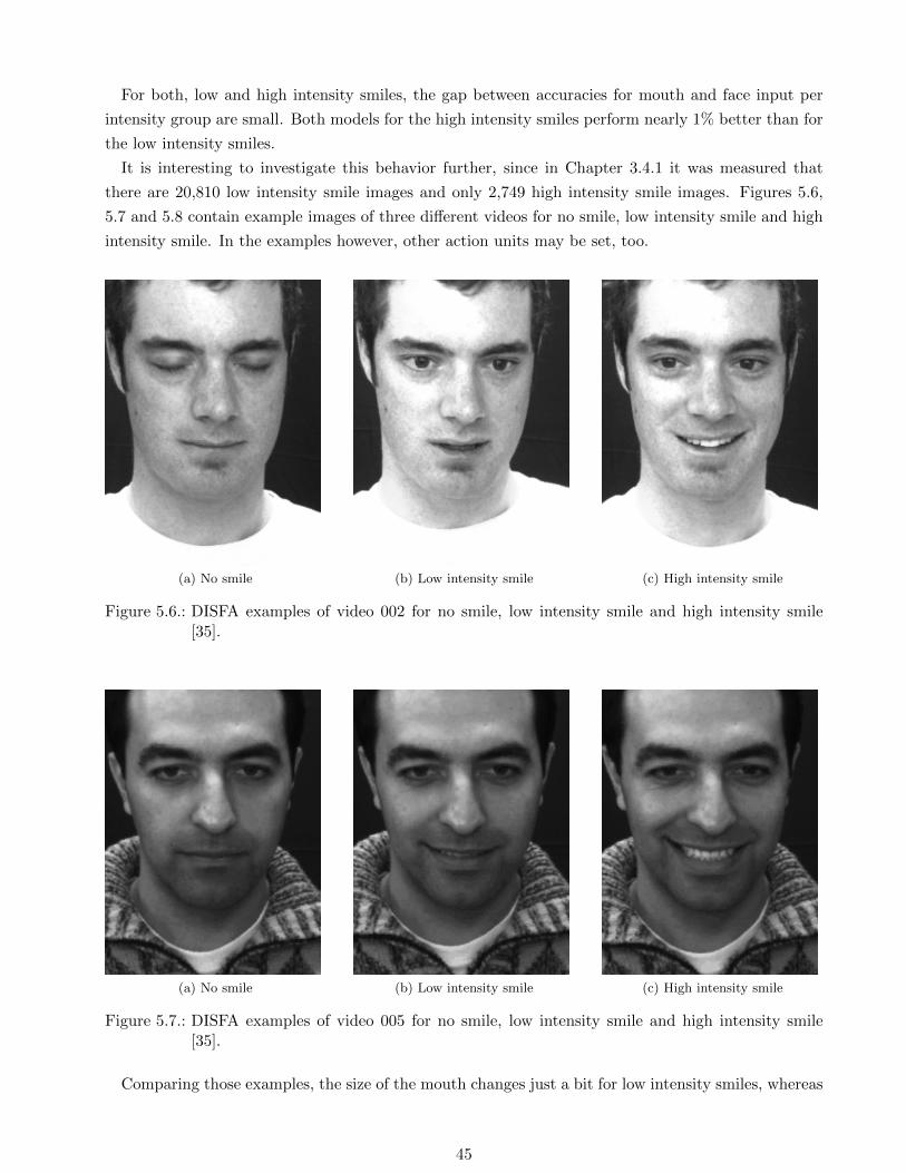
For both, low and high intensity smiles, the gap between accuracies for mouth and face input per
intensity group are small. Both models for the high intensity smiles perform nearly 1% better than for
the low intensity smiles.
It is interesting to investigate this behavior further, since in Chapter 3.4.1 it was measured that
there are 20,810 low intensity smile images and only 2,749 high intensity smile images. Figures 5.6,
5.7 and 5.8 contain example images of three different videos for no smile, low intensity smile and high
intensity smile. In the examples however, other action units may be set, too.
(a) No smile (b) Low intensity smile (c) High intensity smile
Figure 5.6.: DISFA examples of video 002 for no smile, low intensity smile and high intensity smile[35].
(a) No smile (b) Low intensity smile (c) High intensity smile
Figure 5.7.: DISFA examples of video 005 for no smile, low intensity smile and high intensity smile[35].
Comparing those examples, the size of the mouth changes just a bit for low intensity smiles, whereas
45
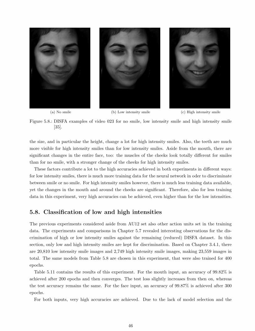
(a) No smile (b) Low intensity smile (c) High intensity smile
Figure 5.8.: DISFA examples of video 023 for no smile, low intensity smile and high intensity smile[35].
the size, and in particular the height, change a lot for high intensity smiles. Also, the teeth are much
more visible for high intensity smiles than for low intensity smiles. Aside from the mouth, there are
significant changes in the entire face, too: the muscles of the cheeks look totally different for smiles
than for no smile, with a stronger change of the cheeks for high intensity smiles.
These factors contribute a lot to the high accuracies achieved in both experiments in different ways:
for low intensity smiles, there is much more training data for the neural network in oder to discriminate
between smile or no smile. For high intensity smiles however, there is much less training data available,
yet the changes in the mouth and around the cheeks are significant. Therefore, also for less training
data in this experiment, very high accuracies can be achieved, even higher than for the low intensities.
5.8. Classification of low and high intensities
The previous experiments considered aside from AU12 set also other action units set in the training
data. The experiments and comparisons in Chapter 5.7 revealed interesting observations for the dis-
crimination of high or low intensity smiles against the remaining (reduced) DISFA dataset. In this
section, only low and high intensity smiles are kept for discrimination. Based on Chapter 3.4.1, there
are 20,810 low intensity smile images and 2,749 high intensity smile images, making 23,559 images in
total. The same models from Table 5.8 are chosen in this experiment, that were also trained for 400
epochs.
Table 5.11 contains the results of this experiment. For the mouth input, an accuracy of 99.82% is
achieved after 200 epochs and then converges. The test loss slightly increases from then on, whereas
the test accuracy remains the same. For the face input, an accuracy of 99.87% is achieved after 300
epochs.
For both inputs, very high accuracies are achieved. Due to the lack of model selection and the
46
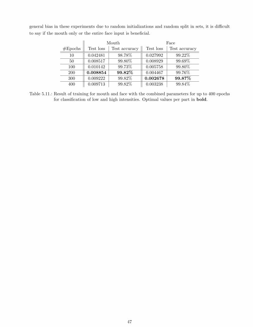
general bias in these experiments due to random initializations and random split in sets, it is difficult
to say if the mouth only or the entire face input is beneficial.
Mouth Face#Epochs Test loss Test accuracy Test loss Test accuracy
10 0.042481 98.78% 0.027992 99.22%
50 0.008517 99.80% 0.008929 99.69%
100 0.010142 99.73% 0.005758 99.80%
200 0.008854 99.82% 0.004467 99.76%
300 0.009222 99.82% 0.002678 99.87%
400 0.009713 99.82% 0.003238 99.84%
Table 5.11.: Result of training for mouth and face with the combined parameters for up to 400 epochsfor classification of low and high intensities. Optimal values per part in bold.
47
6. Conclusions and future work
Deep learning is a set of powerful machine learning algorithms and concepts with groundbreaking
success for the last ten years. The main benefit of deep neural networks are their ability to learn
complex non-linear hypothesis without the need of explicitly modeling features, but rather learning
them from data. Convolutional networks allow to handle distortions, such as translation and rotation
in the input, which occurs frequently in computer vision. Applied to action unit recognition and
smile recognition in particular, a deep convolutional neural network model with an overall accuracy of
99.45% significantly outperforms existing approaches with accuracies ranging from 65.55% to 79.67%.
The network parameter values are subject to extensive model selection. Various variations of this
experiment are run, such as retaining less neutral images or only high or low intensities or classifying
into low or high intensities. For all experiments, very high accuracies above 98.90% are achieved, too.
Choosing the entire face as input or just the mouth only led to minor differences in the accuracies, not
generally favoring either input.
The proposed temporal part using LSTMs was not implemented due to the high accuracies achieved.
It would however be interesting to implement it in the future in order to predict smiles in image
sequences. There are many further topics worth to be investigated. For example, instead of one CNN
being trained on the entire face or the mouth, multiple CNNs could be trained on different regions of
the face. Possible regions are the mouth, the nose and both eyes. A specialized CNN could be trained
for each region allowing to generalize better because of the lower number of parameters in each network.
The CNNs can then be combined using a Shape Boltzmann Machine [9]. Furthermore, in order to
understand the networks better and to do informedly better than blind model selection, it would be
interesting to visualize the units of a network to understand what they learned to detect. This can
help to work well on a variety of action units other than smile. In this thesis, the mouth was compared
to the entire face, for which no significant difference was detected. It would however, be interesting to
investigate this more by comparing the mouth to the face excluding the mouth. So far, the existing
model has been used for classification. In a next step, it can be adopted to regression of action unit
intensities or even valence-arousal [43]. To date, stochastic gradient descent is the preferred training
algorithm for neural networks, as discovered by LeCun in the 1980s and 1990s [31]. Overall, stochastic
gradient descent performs well on deep neural networks, yet it would be interesting to investigate if
LeCun’s observation still holds for deep neural networks. Therefore, stochastic gradient descent should
be compared to a variety of other optimization algorithms, such as Gaussian Newton or Quasi Newton
methods when training deep neural networks.
48
Bibliography
[1] Baccouche, Moez; Mamalet, Franck; Wolf, Christian; Garcia, Christophe and Baskurt, Atilla:
Spatio-Temporal Convolutional Sparse Auto-Encoder for Sequence Classification. 2012.
[2] Banziger, T.; Mortillaro, M. and Scherer, K.R.: Introducing the Geneva Multimodal Expression
corpus for experimental research on emotion perception. Emotion, 12(5), 1161-1179. 2012.
[3] Bergstra, J.; Breuleux, O.; Bastien, F.; Lamblin, P.; Pascanu, R.; Desjardins, G.; Turian, J.;
Warde-Farley, D. and Bengio, Y.: Theano: A CPU and GPU Math Expression Compiler.
Proceedings of the Python for Scientific Computing Conference (SciPy) 2010. June 30 - July 3,
Austin, TX. 2010.
[4] Bishop, Christopher M.: Pattern Recognition and Machine Learning. Springer. 2007.
[5] Deng, Li and Yu, Dong: Deep Learning Methods and Applications. Foundations and Trends in
Signal Processing, 7 (3-4), 197-387. 2014.
[6] Ekman, P. and Friesen, W.: Facial Action Coding System: A Technique for the Measurement
of Facial Movement. Consulting Psychologists Press, Palo Alto. 1978.
[7] Erhan, Dumitru; Manzagol, Pierre-Antoine; Bengio, Yoshua; Bengio, Samy and Vincent, Pascal:
The Difficulty of Training Deep Architectures and the Effect of Unsupervised Pre-Training.
Twelfth International Conference on Artificial Intelligence and Statistics (AISTATS). 2009.
[8] Erhan, Dumitru; Bengio, Yoshua; Courville, Aaron; Manzagol, Pierre-Antoine; Vincent, Pascal
and Bengio, Samy: Why Does Unsupervised Pre-training Help Deep Learning?. Journal of
Machine Learning Research, 11 (Feb), 625-660. 2010.
[9] Eslami, S. M. Ali et al.: The Shape Boltzmann Machine: A Strong Model of Object Shape.
International Journal of Computer Vision. Volume 107, Issue 2, pp 155-176. 2014.
[10] GeForce: GeForce GTX TITAN Black.
http://www.geforce.co.uk/hardware/desktop-gpus/geforce-gtx-titan-black.
Retrieved: August 17, 2015.
[11] Github: craffel/nntools. http://github.com/craffel/nntools. Retrieved: August 17, 2015.
[12] Glauner, Patrick: Comparison of Training Methods for Deep Neural Networks. Imperial College
London, London, UK. arXiv:1504.06825. 2015.
[13] Glauner, Patrick: Deep Neural Networks for Computer Vision. Ocado, Hatfield, UK. 2015.
49

[14] Glorot, Xavier; Bordes, Antoine and Bengio, Yoshua: Deep Sparse Rectifier Neural Networks.
Proceedings of the Fourteenth International Conference on Artificial Intelligence and Statistics
(AISTATS-11). Pages: 315-323. 2011.
[15] Graves, A. and Jaitly, N.: Towards end-to-end speech recognition with recurrent neural
networks. In Proc. ICML, pages 1764-1772. Beijing, China. 2014.
[16] Gudi, Amogh; Tasli, H. Emrah; den Uyl, Tim M. and Maroulis, Andreas: Deep Learning based
FACS Action Unit Occurrence and Intensity Estimation. Vicarious Perception Technologies.
Amsterdam, The Netherlands. 2015.
[17] Hannun, A.; Case, C.; Casper, J., Catanzaro, B.; Diamos, G., Elsen, E.; Prenger, R.; Satheesh,
S.; Sengupta, S.; Coates, A. et al.: Deepspeech: Scaling up end-to-end speech recognition. 2014.
[18] Hinton, Geoffrey: A Practical Guide to Training Restricted Boltzmann Machines. UTML TR
2010-003, University of Toronto. 2010.
[19] Hinton, Geoffrey et al.: Deep Neural Networks for Acoustic Modeling in Speech Recognition.
IEEE Signal Processing Magazine, 29 (6), 82-97. 2012.
[20] Hinton, Geoffrey and Salakhutdinov, R.: Reducing the dimensionality of data with neural
networks. Science, 313 (5786), 504-507. 2006.
[21] Hochreiter, Sepp and Schmidhuber, Juergen: Long short-term memory. Neural Computation 9
(8): 1735-1780. 1997.
[22] Ioffe, Sergey and Szegedy, Christian: Batch Normalization: Accelerating Deep Network
Training by Reducing Internal Covariate Shift. Google. 2015.
[23] Ji, Shuiwang; Xu, Wei; Yang, Ming; Yu, Kai: 3D Convolutional Neural Networks for Human
Action Recognition. IEEE Transactions on Pattern Analysis and Machine Intelligence, 35 (1),
221 - 231. 2012.
[24] Jia, Yangqing; Shelhamer, Evan; Donahue, Jeff; Karayev, Sergey; Long, Jonathan; Girshick,
Ross; Guadarrama, Sergio and Darrell, Trevor: Caffe: Convolutional Architecture for Fast
Feature Embedding. arXiv:1408.5093. 2014.
[25] Kaggle: Emotion and identity detection from face images.
http://inclass.kaggle.com/c/facial-keypoints-detector. Retrieved: April 15, 2015.
[26] Kahou, Samira Ebrahimi et al.: EmoNets: Multimodal deep learning approaches for emotion
recognition in video. 2015.
[27] Karpathy, Andrej; Toderici, George; Shetty, Sanketh; Leung, Thomas; Sukthankar, Rahul and
Fei-Fei, Li: Large-scale Video Classification with Convolutional Neural Networks. 2014.
[28] Larochelle, Hugo; Lajoie, Isabelle and Bengio, Yoshua: Stacked Denoising Autoencoders:
Learning Useful Representations in a Deep Network with a Local Denoising Criterion. The
Journal of Machine Learning Research, 11, 3371-3408. 2010.
50
[29] Le, Quoc; Ranzato, Marc’Aurelio; Monga, Rajat; Devin, Matthieu; Chen, Kai; Corrado, Greg;
Dean, Jeff and Ng, Andrew: Building high-level features using large scale unsupervised
learning. International Conference in Machine Learning. 2012.
[30] LeCun, Yann et al.: LeNet-5, convolutional neural networks.
http://yann.lecun.com/exdb/lenet/. Retrieved: April 22, 2015
[31] LeCun, Yann: Research profile. http://yann.lecun.com/ex/research/index.html.
Retrieved: February 28, 2015.
[32] Lucy, P.; Cohn, J. F.; Prkachin, K. M.; Solomon, P. and Matthrews, I.: Painful data: The
UNBC-McMaster Shoulder Pain Expression Archive Database. IEEE International Conference
on Automatic Face and Gesture Recognition (FG2011). 2011.
[33] Mansimov, Elman; Srivastava, Nitish and Salakhutdinov, Ruslan: Initialization Strategies of
Spatio-Temporal Convolutional Neural Networks. 2015.
[34] van Merrienboer, Bart; Bahdanau, Dzmitry; Dumoulin, Vincent; Serdyuk, Dmitriy;
Warde-Farley, David; Chorowski, Jan and Bengio, Yoshua: Blocks and Fuel: Frameworks for
deep learning. http://arxiv.org/abs/1506.00619. 2015.
[35] Mavadati, S.M.; Mahoor M.H.; Bartlett, K; Trinh, P. and Cohn, J.F.: Disfa: A spontaneous
facial action intensity database. IEEE Transactions on Affective Computing, page 1. 2013.
[36] McDuff, Daniel; El Kaliouby, Rana; Senechal, Thibaud; Amr, May; Cohn, Jeffrey; Picard,
Rosalind and Affectiva: Affectiva-MIT Facial Expression Dataset (AM-FED): Naturalistic and
Spontaneous Facial Expressions Collected ”In-the-Wild”. Proceeding CVPRW ’13 Proceedings
of the 2013 IEEE Conference on Computer Vision and Pattern Recognition Workshops, pages
881-888. 2013.
[37] Mitchell, Tom: Machine Learning. McGraw Hill. 1997.
[38] Nair, Vinod and Hinton, Geoffrey E.: Rectified Linear Units Improve Restricted Boltzmann.
2010.
[39] Ng, Andrew: Feature selection, L1 vs. L2 regularization, and rotational invariance. Stanford.
2004.
[40] Ng, Andrew: Machine Learning. Coursera. 2014.
[41] Ng, Andrew et al.: Deep Learning Tutorial. http://deeplearning.stanford.edu/tutorial/.
Retrieved: February 27, 2015.
[42] Ng, Joe Yue-Hei; Vinyals, Oriol; Hausknecht, Matthew; Monga, Rajat; Vijayanarasimhan,
Sudheendra and Toderici, George: Beyond Short Snippets: Deep Networks for Video
Classification. 2015.
51
[43] Nicolaou, Mihalis A.; Pavlovic, Vladimir and Pantic, Maja: Dynamic Probabilistic CCA for
Analysis of Affective Behavior and Fusion of Continuous Annotations. IEEE TRANSACTIONS
ON PATTERN ANALYSIS AND MACHINE INTELLIGENCE. VOL. 36, NO. 7. 2014.
[44] Norvig, Peter and Russel, Stuart: Artificial Intelligence: A Modern Approach. Prentice Hall.
Third Edition. 2009.
[45] NVIDIA: TESLA. http://www.nvidia.com/object/tesla-servers.html. Retrieved: August
20, 2015.
[46] Palm, Rasmus Berg: DeepLearnToolbox.
http://github.com/rasmusbergpalm/DeepLearnToolbox. Retrieved: April 22, 2015.
[47] Petridis, S.; Martinez, B. and Pantic, M.: The MAHNOB Laughter Database. Image and
Vision Computing Journal. 31(2): pp. 186 - 202. 2013.
[48] Pigou, Lionel; van den Oord, Aaron; Dieleman, Sander; Van Herreweghe, Mieke and Dambre,
Joni: Beyond Temporal Pooling: Recurrence and Temporal Convolutions for Gesture
Recognition in Video. Ghent University, Belgium. 2015.
[49] Sainath, T. N.; Vinyals, O.; Senior, A. and Sak, H.: Convolutional, Long Short-Term Memory,
Fully Connected Deep Neural Networks. Proc. ICASSP. 2015.
[50] Sourceforge: CURRENNT. http://sourceforge.net/projects/currennt. Retrieved: August
17, 2015.
[51] Sourceforge: RNNLIB. http://sourceforge.net/p/rnnl. Retrieved: August 17, 2015.
[52] Springenberg, Jost Tobias; Dosovitskiy, Alexey; Brox, Thomas and Riedmiller, Martin: Striving
for Simplicity: The All Convolutional Net. University of Freiburg, Germany. arXiv:1504.06825.
2015.
[53] Srivastava, Nitish; Hinton, Geoffrey; Krizhevsky, Alex; Sutskever, Ilya and Salakhutdinov,
Ruslan: Dropout: A Simple Way to Prevent Neural Networks from Overfitting. The Journal of
Machine Learning Research, 15, 1929-1958, 2014.
[54] Srivastava, Nitish; Mansimov, Elman and Salakhutdinov, Ruslan: Unsupervised Learning of
Video Representations using LSTMs. University of Toronto. 2015.
[55] Tang, Y.: Challenges in Representation Learning: Facial Expression Recognition Challenge
Implementation. University of Toronto. 2013.
[56] The Analytics Store: Deep Learning. http://theanalyticsstore.com/deep-learning/.
Retrieved: March 1, 2015.
[57] Todorovic, Sinisa: Recent Research Topics. Oregon State University.
http://web.engr.oregonstate.edu/~sinisa/. Retrieved: August 1, 2015.
52

[58] Yan, Wen-Jing; Wu, Qi; Liu, Yong-Jin; Wang, Su-Jing and Fu, Xiaolan: CASME database: A
dataset of spontaneous micro-expressions collected from neutralized faces. Automatic Face and
Gesture Recognition (FG), 2013 10th IEEE International Conference and Workshops on. 2013.
53
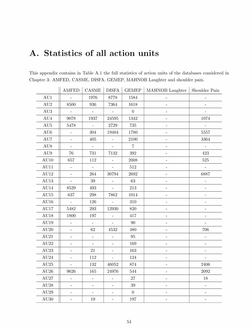
A. Statistics of all action units
This appendix contains in Table A.1 the full statistics of action units of the databases considered in
Chapter 3: AMFED, CASME, DISFA, GEMEP, MAHNOB Laughter and shoulder pain.
AMFED CASME DISFA GEMEP MAHNOB Laughter Shoulder Pain
AU1 - 1976 8778 1584 - -
AU2 8500 936 7364 1618 - -
AU3 - - - 0 - -
AU4 9078 1937 24595 1342 - 1074
AU5 5478 - 2729 735 - -
AU6 - 304 19484 1780 - 5557
AU7 - 405 - 2100 - 3364
AU8 - - - 7 - -
AU9 76 731 7132 392 - 423
AU10 657 112 - 2008 - 525
AU11 - - - 512 - -
AU12 - 264 30794 2692 - 6887
AU13 - 39 - 63 - -
AU14 8529 493 - 213 - -
AU15 637 298 7862 1014 - -
AU16 - 126 - 310 - -
AU17 5482 293 12930 820 - -
AU18 1800 197 - 417 - -
AU19 - - - 90 - -
AU20 - 62 4532 480 - 706
AU21 - - - 95 - -
AU22 - - - 169 - -
AU23 - 21 - 163 - -
AU24 - 112 - 124 - -
AU25 - 132 46052 874 - 2406
AU26 9626 165 24976 544 - 2092
AU27 - - - 27 - 18
AU28 - - - 39 - -
AU29 - - - 0 - -
AU30 - 19 - 197 - -
54
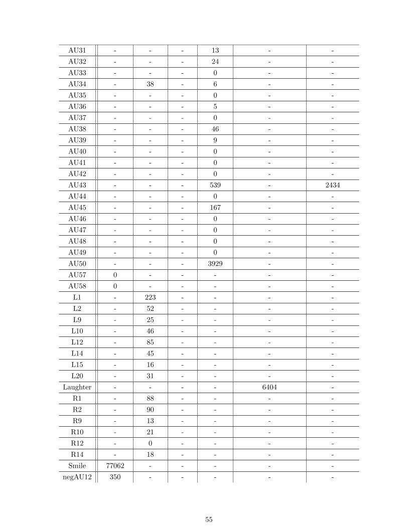
AU31 - - - 13 - -
AU32 - - - 24 - -
AU33 - - - 0 - -
AU34 - 38 - 6 - -
AU35 - - - 0 - -
AU36 - - - 5 - -
AU37 - - - 0 - -
AU38 - - - 46 - -
AU39 - - - 9 - -
AU40 - - - 0 - -
AU41 - - - 0 - -
AU42 - - - 0 - -
AU43 - - - 539 - 2434
AU44 - - - 0 - -
AU45 - - - 167 - -
AU46 - - - 0 - -
AU47 - - - 0 - -
AU48 - - - 0 - -
AU49 - - - 0 - -
AU50 - - - 3929 - -
AU57 0 - - - - -
AU58 0 - - - - -
L1 - 223 - - - -
L2 - 52 - - - -
L9 - 25 - - - -
L10 - 46 - - - -
L12 - 85 - - - -
L14 - 45 - - - -
L15 - 16 - - - -
L20 - 31 - - - -
Laughter - - - - 6404 -
R1 - 88 - - - -
R2 - 90 - - - -
R9 - 13 - - - -
R10 - 21 - - - -
R12 - 0 - - - -
R14 - 18 - - - -
Smile 77062 - - - - -
negAU12 350 - - - - -
55

Table A.1.: Complete statistics of action units in databases: an integer denotes the number of framesin which an action unit is set (intensity > 0). A hyphen indicates that an action unit isnot available in a database.
56

B. Training time of networks
This appendix contains the full statistics of median epoch durations of the different convolutional
models trained in Chapter 5. For none of the experiments, a significant spread of the epoch durations
was observed, therefore only the median is available in this chapter.
B.1. Full dataset
Table B.1 shows that training time mostly depends on the number of convolutional and pooling layers.
Different levels of dropout have no significant impact on the duration of an epoch. Training time is
slightly less when dropout is disabled totally for p = 0. The number of hidden units in the tested range
has only a minor effect on the training time, but grows slowly with the increased values. Significantly
larger number of units per layer are likely to change the training time stronger.
#Convs #Hidden layers #Units hidden layers Dropout Mouth Face
1 1 100 0.5 46.889 52.367
2 1 100 0.5 110.956 123.221
3 1 100 0.5 135.143 150.961
1 2 100 0.5 46.844 52.382
1 3 100 0.5 47.029 51.993
1 1 200 0.5 49.069 54.663
1 1 300 0.5 50.632 56.578
1 1 400 0.5 54.916 61.095
1 1 100 0 45.034 49.843
1 1 100 0.1 47.353 52.297
1 1 100 0.7 47.107 52.247
Table B.1.: Median epoch duration in seconds during model selection of different architectures. Forfull dataset.
Table B.2 contains the median epoch duration for the final models selected for mouth and face input.
A comparison of the training time is not possible, as the selected values are very different and because
the number of input pixels is different, too.
#Convs #Hidden layers #Units hidden layers Dropout Mouth Face
2 2 400 0.1 112.436 -
1 1 400 0 - 58.823
Table B.2.: Median epoch duration in seconds for final models selected. For full dataset.
57
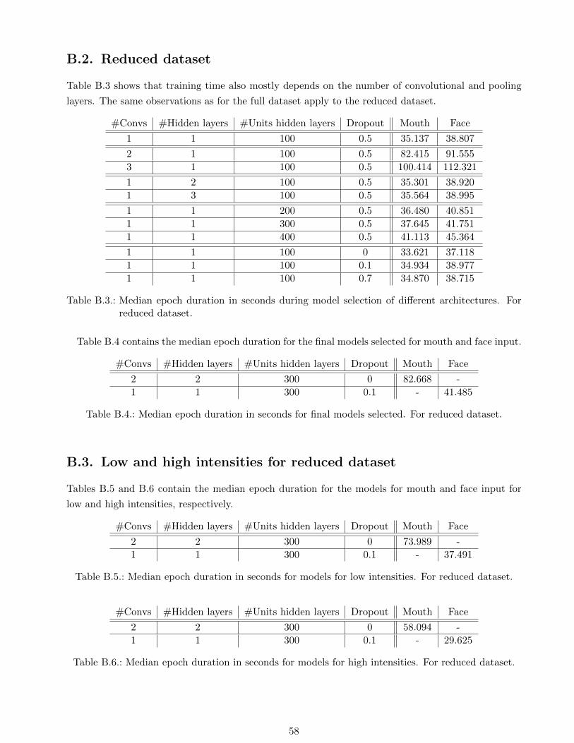
B.2. Reduced dataset
Table B.3 shows that training time also mostly depends on the number of convolutional and pooling
layers. The same observations as for the full dataset apply to the reduced dataset.
#Convs #Hidden layers #Units hidden layers Dropout Mouth Face
1 1 100 0.5 35.137 38.807
2 1 100 0.5 82.415 91.555
3 1 100 0.5 100.414 112.321
1 2 100 0.5 35.301 38.920
1 3 100 0.5 35.564 38.995
1 1 200 0.5 36.480 40.851
1 1 300 0.5 37.645 41.751
1 1 400 0.5 41.113 45.364
1 1 100 0 33.621 37.118
1 1 100 0.1 34.934 38.977
1 1 100 0.7 34.870 38.715
Table B.3.: Median epoch duration in seconds during model selection of different architectures. Forreduced dataset.
Table B.4 contains the median epoch duration for the final models selected for mouth and face input.
#Convs #Hidden layers #Units hidden layers Dropout Mouth Face
2 2 300 0 82.668 -
1 1 300 0.1 - 41.485
Table B.4.: Median epoch duration in seconds for final models selected. For reduced dataset.
B.3. Low and high intensities for reduced dataset
Tables B.5 and B.6 contain the median epoch duration for the models for mouth and face input for
low and high intensities, respectively.
#Convs #Hidden layers #Units hidden layers Dropout Mouth Face
2 2 300 0 73.989 -
1 1 300 0.1 - 37.491
Table B.5.: Median epoch duration in seconds for models for low intensities. For reduced dataset.
#Convs #Hidden layers #Units hidden layers Dropout Mouth Face
2 2 300 0 58.094 -
1 1 300 0.1 - 29.625
Table B.6.: Median epoch duration in seconds for models for high intensities. For reduced dataset.
58

B.4. Classification of low and high intensities
Table B.7 contains the median epoch duration for the models for mouth and face input.
#Convs #Hidden layers #Units hidden layers Dropout Mouth Face
2 2 300 0 19.865 -
1 1 300 0.1 - 10.071
Table B.7.: Median epoch duration in seconds for models for classification of low and high intensities.
59
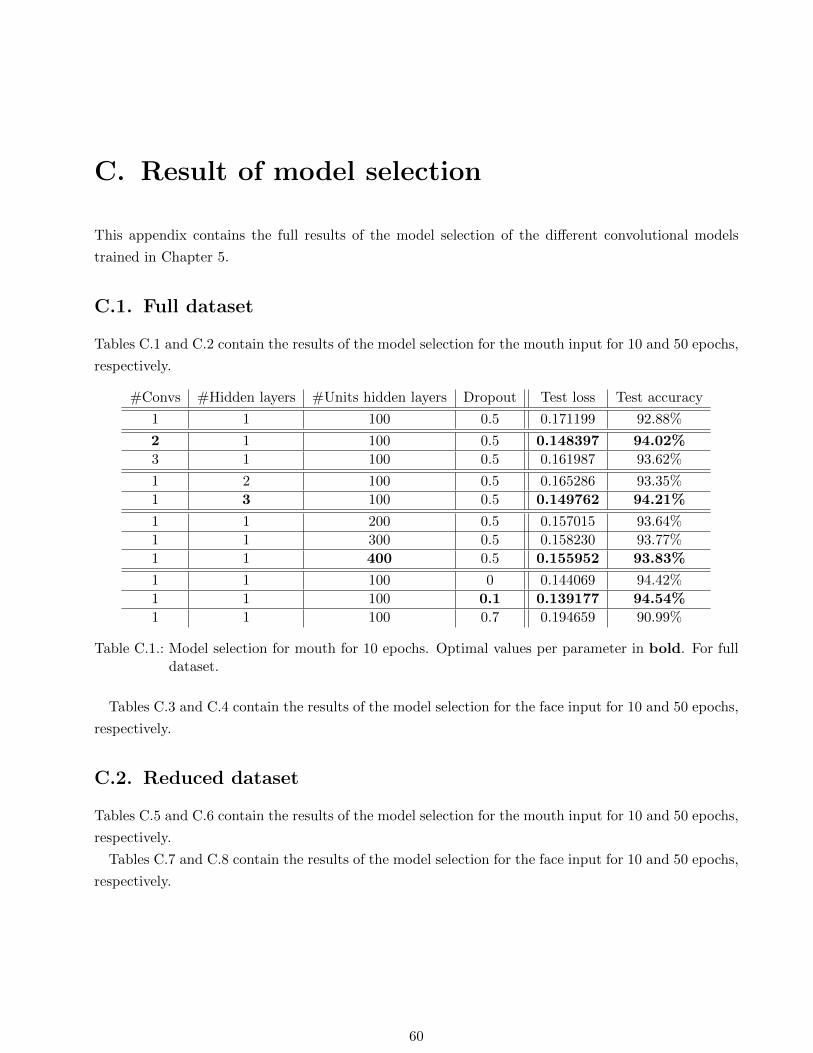
C. Result of model selection
This appendix contains the full results of the model selection of the different convolutional models
trained in Chapter 5.
C.1. Full dataset
Tables C.1 and C.2 contain the results of the model selection for the mouth input for 10 and 50 epochs,
respectively.
#Convs #Hidden layers #Units hidden layers Dropout Test loss Test accuracy
1 1 100 0.5 0.171199 92.88%
2 1 100 0.5 0.148397 94.02%
3 1 100 0.5 0.161987 93.62%
1 2 100 0.5 0.165286 93.35%
1 3 100 0.5 0.149762 94.21%
1 1 200 0.5 0.157015 93.64%
1 1 300 0.5 0.158230 93.77%
1 1 400 0.5 0.155952 93.83%
1 1 100 0 0.144069 94.42%
1 1 100 0.1 0.139177 94.54%
1 1 100 0.7 0.194659 90.99%
Table C.1.: Model selection for mouth for 10 epochs. Optimal values per parameter in bold. For fulldataset.
Tables C.3 and C.4 contain the results of the model selection for the face input for 10 and 50 epochs,
respectively.
C.2. Reduced dataset
Tables C.5 and C.6 contain the results of the model selection for the mouth input for 10 and 50 epochs,
respectively.
Tables C.7 and C.8 contain the results of the model selection for the face input for 10 and 50 epochs,
respectively.
60
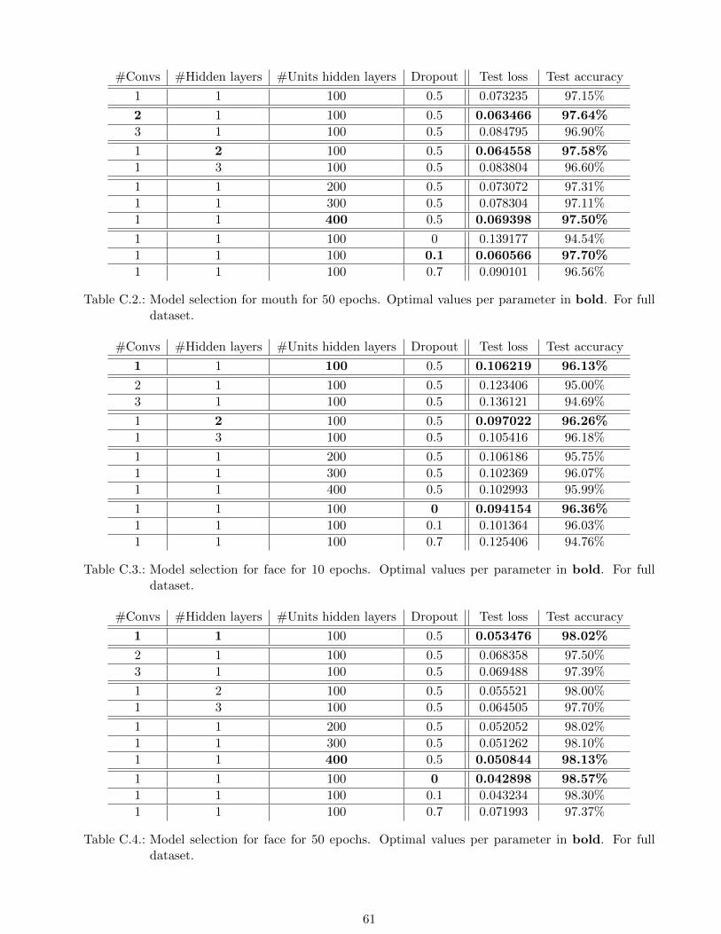
#Convs #Hidden layers #Units hidden layers Dropout Test loss Test accuracy
1 1 100 0.5 0.073235 97.15%
2 1 100 0.5 0.063466 97.64%
3 1 100 0.5 0.084795 96.90%
1 2 100 0.5 0.064558 97.58%
1 3 100 0.5 0.083804 96.60%
1 1 200 0.5 0.073072 97.31%
1 1 300 0.5 0.078304 97.11%
1 1 400 0.5 0.069398 97.50%
1 1 100 0 0.139177 94.54%
1 1 100 0.1 0.060566 97.70%
1 1 100 0.7 0.090101 96.56%
Table C.2.: Model selection for mouth for 50 epochs. Optimal values per parameter in bold. For fulldataset.
#Convs #Hidden layers #Units hidden layers Dropout Test loss Test accuracy
1 1 100 0.5 0.106219 96.13%
2 1 100 0.5 0.123406 95.00%
3 1 100 0.5 0.136121 94.69%
1 2 100 0.5 0.097022 96.26%
1 3 100 0.5 0.105416 96.18%
1 1 200 0.5 0.106186 95.75%
1 1 300 0.5 0.102369 96.07%
1 1 400 0.5 0.102993 95.99%
1 1 100 0 0.094154 96.36%
1 1 100 0.1 0.101364 96.03%
1 1 100 0.7 0.125406 94.76%
Table C.3.: Model selection for face for 10 epochs. Optimal values per parameter in bold. For fulldataset.
#Convs #Hidden layers #Units hidden layers Dropout Test loss Test accuracy
1 1 100 0.5 0.053476 98.02%
2 1 100 0.5 0.068358 97.50%
3 1 100 0.5 0.069488 97.39%
1 2 100 0.5 0.055521 98.00%
1 3 100 0.5 0.064505 97.70%
1 1 200 0.5 0.052052 98.02%
1 1 300 0.5 0.051262 98.10%
1 1 400 0.5 0.050844 98.13%
1 1 100 0 0.042898 98.57%
1 1 100 0.1 0.043234 98.30%
1 1 100 0.7 0.071993 97.37%
Table C.4.: Model selection for face for 50 epochs. Optimal values per parameter in bold. For fulldataset.
61
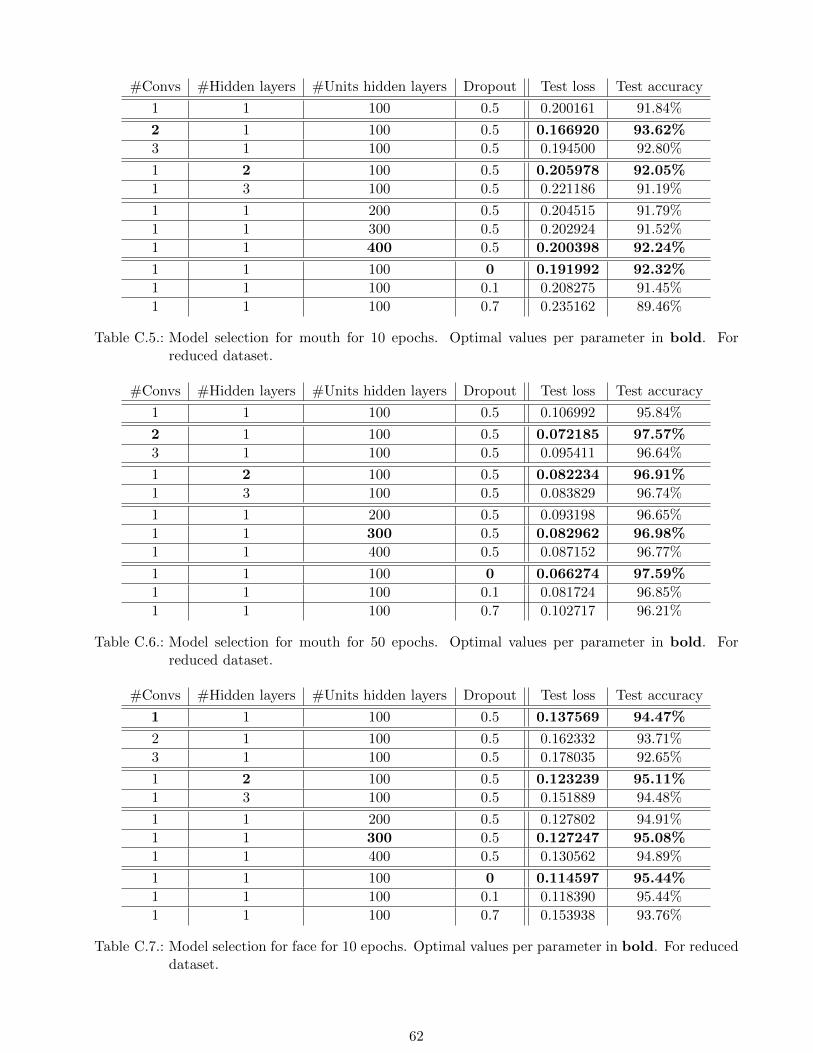
#Convs #Hidden layers #Units hidden layers Dropout Test loss Test accuracy
1 1 100 0.5 0.200161 91.84%
2 1 100 0.5 0.166920 93.62%
3 1 100 0.5 0.194500 92.80%
1 2 100 0.5 0.205978 92.05%
1 3 100 0.5 0.221186 91.19%
1 1 200 0.5 0.204515 91.79%
1 1 300 0.5 0.202924 91.52%
1 1 400 0.5 0.200398 92.24%
1 1 100 0 0.191992 92.32%
1 1 100 0.1 0.208275 91.45%
1 1 100 0.7 0.235162 89.46%
Table C.5.: Model selection for mouth for 10 epochs. Optimal values per parameter in bold. Forreduced dataset.
#Convs #Hidden layers #Units hidden layers Dropout Test loss Test accuracy
1 1 100 0.5 0.106992 95.84%
2 1 100 0.5 0.072185 97.57%
3 1 100 0.5 0.095411 96.64%
1 2 100 0.5 0.082234 96.91%
1 3 100 0.5 0.083829 96.74%
1 1 200 0.5 0.093198 96.65%
1 1 300 0.5 0.082962 96.98%
1 1 400 0.5 0.087152 96.77%
1 1 100 0 0.066274 97.59%
1 1 100 0.1 0.081724 96.85%
1 1 100 0.7 0.102717 96.21%
Table C.6.: Model selection for mouth for 50 epochs. Optimal values per parameter in bold. Forreduced dataset.
#Convs #Hidden layers #Units hidden layers Dropout Test loss Test accuracy
1 1 100 0.5 0.137569 94.47%
2 1 100 0.5 0.162332 93.71%
3 1 100 0.5 0.178035 92.65%
1 2 100 0.5 0.123239 95.11%
1 3 100 0.5 0.151889 94.48%
1 1 200 0.5 0.127802 94.91%
1 1 300 0.5 0.127247 95.08%
1 1 400 0.5 0.130562 94.89%
1 1 100 0 0.114597 95.44%
1 1 100 0.1 0.118390 95.44%
1 1 100 0.7 0.153938 93.76%
Table C.7.: Model selection for face for 10 epochs. Optimal values per parameter in bold. For reduceddataset.
62

#Convs #Hidden layers #Units hidden layers Dropout Test loss Test accuracy
1 1 100 0.5 0.067837 97.44%
2 1 100 0.5 0.082837 96.77%
3 1 100 0.5 0.090266 96.64%
1 2 100 0.5 0.069571 97.31%
1 3 100 0.5 0.099563 95.91%
1 1 200 0.5 0.065923 97.41%
1 1 300 0.5 0.062300 97.58%
1 1 400 0.5 0.062894 97.54%
1 1 100 0 0.083884 96.99%
1 1 100 0.1 0.049972 98.16%
1 1 100 0.7 0.091003 96.62%
Table C.8.: Model selection for face for 50 epochs. Optimal values per parameter in bold. For reduceddataset.
63
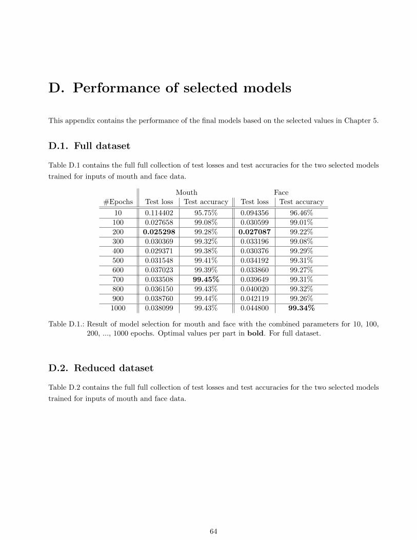
D. Performance of selected models
This appendix contains the performance of the final models based on the selected values in Chapter 5.
D.1. Full dataset
Table D.1 contains the full full collection of test losses and test accuracies for the two selected models
trained for inputs of mouth and face data.
Mouth Face#Epochs Test loss Test accuracy Test loss Test accuracy
10 0.114402 95.75% 0.094356 96.46%
100 0.027658 99.08% 0.030599 99.01%
200 0.025298 99.28% 0.027087 99.22%
300 0.030369 99.32% 0.033196 99.08%
400 0.029371 99.38% 0.030376 99.29%
500 0.031548 99.41% 0.034192 99.31%
600 0.037023 99.39% 0.033860 99.27%
700 0.033508 99.45% 0.039649 99.31%
800 0.036150 99.43% 0.040020 99.32%
900 0.038760 99.44% 0.042119 99.26%
1000 0.038099 99.43% 0.044800 99.34%
Table D.1.: Result of model selection for mouth and face with the combined parameters for 10, 100,200, ..., 1000 epochs. Optimal values per part in bold. For full dataset.
D.2. Reduced dataset
Table D.2 contains the full full collection of test losses and test accuracies for the two selected models
trained for inputs of mouth and face data.
64
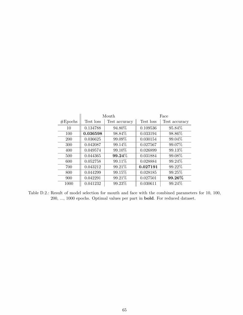
Mouth Face#Epochs Test loss Test accuracy Test loss Test accuracy
10 0.134788 94.80% 0.109536 95.84%
100 0.036598 98.84% 0.033194 98.86%
200 0.036625 99.09% 0.030154 99.04%
300 0.042087 99.14% 0.027567 99.07%
400 0.049574 99.10% 0.026899 99.13%
500 0.044365 99.24% 0.031884 99.08%
600 0.052758 99.11% 0.028884 99.24%
700 0.043212 99.21% 0.027191 99.22%
800 0.044299 99.15% 0.028185 99.25%
900 0.042291 99.21% 0.027501 99.26%
1000 0.041232 99.23% 0.030611 99.24%
Table D.2.: Result of model selection for mouth and face with the combined parameters for 10, 100,200, ..., 1000 epochs. Optimal values per part in bold. For reduced dataset.
65


![Constrained Convolutional Neural Networks for …vgg/rg/slides/ccnn1.pdf · Constrained Convolutional Neural Networks for Weakly Supervised Segmentation ... [CCNN] Convolutional Neural](https://img.dokumen.tips/doc/110x75/5baa6a3809d3f2c9618bd4b3/constrained-convolutional-neural-networks-for-vggrgslidesccnn1pdf-constrained.jpg)