Embed Size (px)
Citation preview

Decoupled Sampling forReal-Time Graphics Pipelines
Jonathan Ragan-Kelley, MIT CSAILJaakko Lehtinen, Jiawen Chen, MIT CSAIL
Michael Doggett, Lund UniversityFrédo Durand, MIT CSAIL
http://bit.ly/DecoupledSampling
Looking at other ways we can evolve the existing graphics pipeline to scale to future workloads more efficiently,I’m going to talk about a project currently in review for Transactions on Graphics.
The current draft is online and public, and includes a lot more detail than I’ll cover here. I’d encourage anyone to check it out at the URL below, or just by Googling for my name.
This is joint work with Jaakko, Kevin, and Frédo from MIT, and Mike Doggett from Lund.(Jaakko is now at NVIDIA Research, where Kevin and I also are for the summer.)

Complex:GeometryVisibilityShading
(cc) Keith MarshallThe real world is complex.
If we want to render realistic, or satisfyingly complex images,we need very detailed: - geometry - what shape things are, - visibility - how & what we actually see of those shapes - shading - what color they appear
© PixarPixar realized this a long time ago.
And in particular they realized that,as we radically increase image complexity, we need to consider fundamental systems concerns from first principlesbased on our target design goals.Just scaling one strategy to the limit often isn't sufficient/efficient.
Specifically, when they set out to pursue the then-audacious goal of rendering CG images of intrinsically compelling complexity, this design goal forced them to rethink the rendering process from the start.
(breathe)so, in a similar vein,Kayvon's just talked about some of the systems challenges in increasing geometric detail.I'm going to focus on managing complexity in visibility and shading.
© Pixar
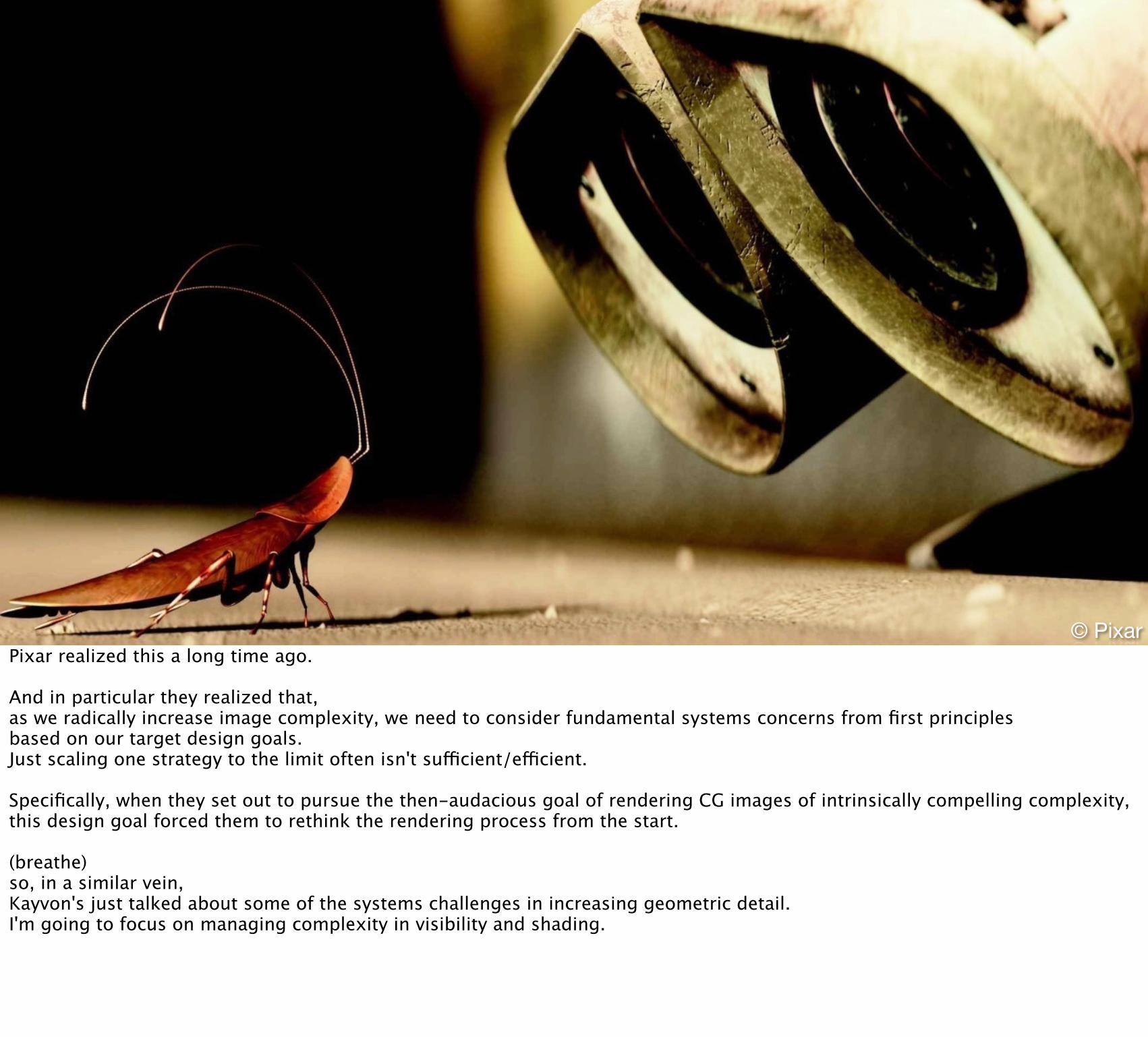
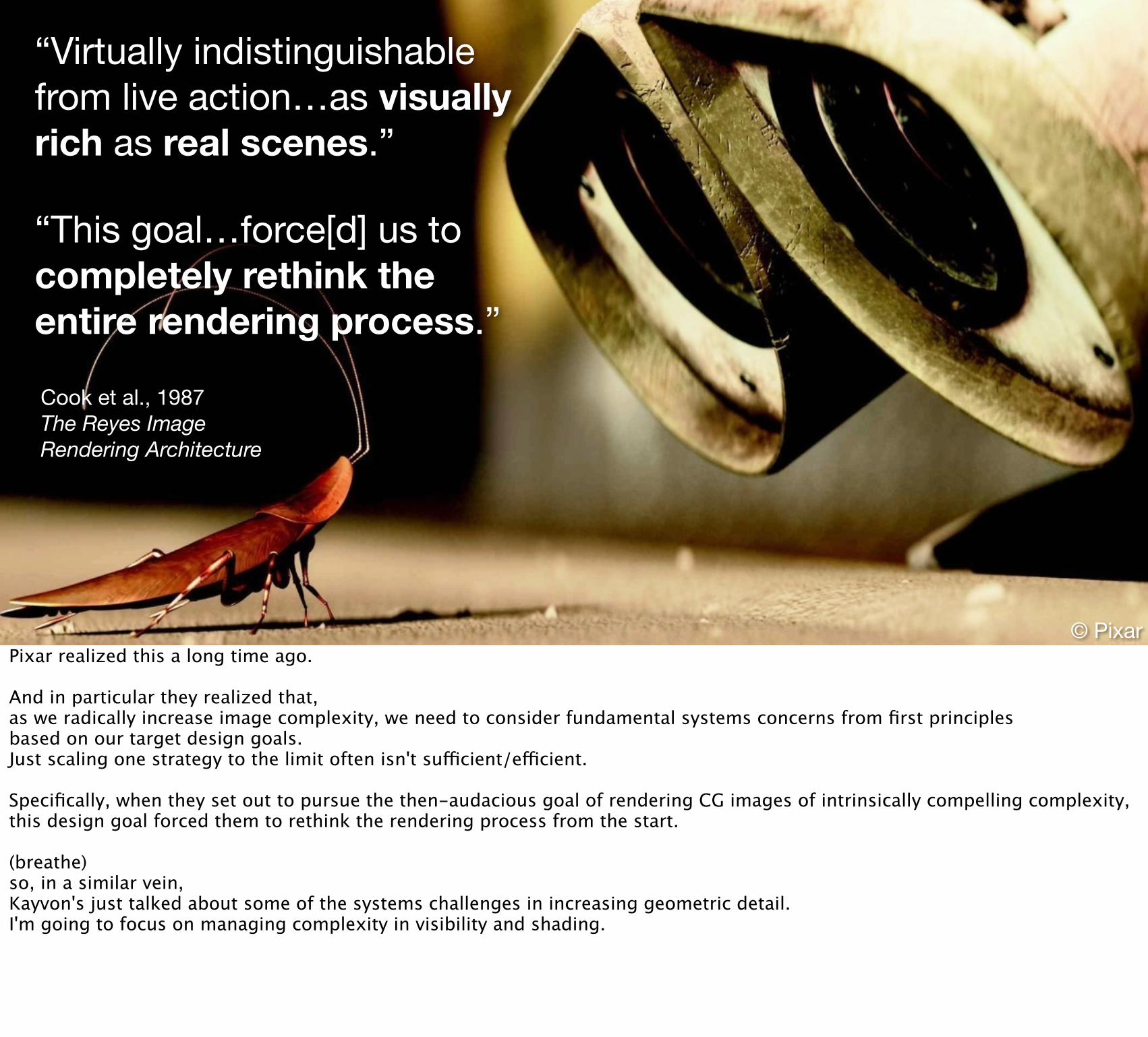
“This goal…force[d] us to completely rethink the entire rendering process.”
“Virtually indistinguishable from live action…as visually rich as real scenes.”
Cook et al., 1987The Reyes Image Rendering Architecture
Pixar realized this a long time ago.
And in particular they realized that,as we radically increase image complexity, we need to consider fundamental systems concerns from first principlesbased on our target design goals.Just scaling one strategy to the limit often isn't sufficient/efficient.
Specifically, when they set out to pursue the then-audacious goal of rendering CG images of intrinsically compelling complexity, this design goal forced them to rethink the rendering process from the start.
(breathe)so, in a similar vein,Kayvon's just talked about some of the systems challenges in increasing geometric detail.I'm going to focus on managing complexity in visibility and shading.

Rendering:Compute what’s visible.Compute what color it is.
So, what is rendering?
When rendering a picture, you fundamentally have to do 2 things:
you have to _compute what's visible_ (visibility)
and you have to _compute what color it appears to be_ (shading)
High quality rendering requires very complex visibility _and_ shading

Complex visibilitymany stochastic point samplesin 5D (space, time, lens aperture)
Complex shadingexpensive evaluationcan be prefiltered
In practice:
visibility varies abruptly and unpredictably, and cannot easily be prefiltered. So complex visibility requires _many (stochastic) samples_ to smoothly resolve fine detail, _including changes in space and time_.
The evaluation of individual samples may be relatively inexpensive, but we need a _lots_ of them.
In contrast,Complex shading requires _very expensive_ evaluation of color at any given point.And unlike visibility, shading often varies relatively smoothly and can be prefiltered—with mip-mapping, for example.
As a result, we'd like to evaluate it _as little as possible_.

Design goals
1. Scale to large numbers of stochastic visibility samples.
2. Shade at the lowest frequency possible.
3. Only shade visible points.
From this, we're left with 3 fundamental goals in defining a system to render images with complex visibility and shading:
It needs to:
- scale to large numbers of stochastic samples, in 5D—not just over the screen, but also lens aperture and time- shade at the lowest frequency possible—often much less than the visibility sampling rate- only shade points which you can actually see—because it's obviously wasteful to compute colors that don't contribute to the final image
- historically this has been a classic "pick 2" dilemma.
The goal of this project is to achieve all 3.

Design goals
1. Scale to large numbers of stochastic visibility samples.
2. Shade at the lowest frequency possible.
3. Only shade visible points.Pick 2
From this, we're left with 3 fundamental goals in defining a system to render images with complex visibility and shading:
It needs to:
- scale to large numbers of stochastic samples, in 5D—not just over the screen, but also lens aperture and time- shade at the lowest frequency possible—often much less than the visibility sampling rate- only shade points which you can actually see—because it's obviously wasteful to compute colors that don't contribute to the final image
- historically this has been a classic "pick 2" dilemma.
The goal of this project is to achieve all 3.
A simple graphics pipeline
Xform Rast Depth-Stencil Shade FB
transformedprimitives
coveredpixels,
shadingsamples
visiblepixels,
shadingsamples
coloredpixels
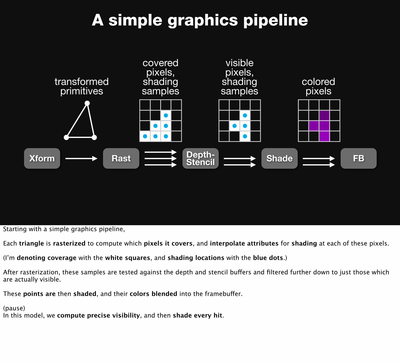
Starting with a simple graphics pipeline,
Each triangle is rasterized to compute which pixels it covers, and interpolate attributes for shading at each of these pixels.
(I’m denoting coverage with the white squares, and shading locations with the blue dots.)
After rasterization, these samples are tested against the depth and stencil buffers and filtered further down to just those which are actually visible.
These points are then shaded, and their colors blended into the framebuffer.
(pause)In this model, we compute precise visibility, and then shade every hit.

Supersampling
Xform Rast Depth-Stencil Shade FB
transformedprimitives
coveredsubpixels,shadingsamples
visiblesubpixels,shadingsamples
coloredsubpixels
You can support antialiasing by supersampling the entire process starting at sample generation.
For each output pixel, we now compute coverage, occlusion, and shading at multiple subpixel locations.

Supersampling generalizes to blur
Xform Rast Depth-Stencil Shade FB
transformedprimitives
coveredsubpixels,shadingsamples
visiblesubpixels,shadingsamples
coloredsubpixels
This naturally generalizes to blur by associating a time and lens location with each visibility sample.Each one sees a view of the triangle at a different point in time, from a different spot on the lens.
When you filter them together, you get motion and defocus blur.
This is what you'd get from a simple supersampling renderer, like a classic distribution ray tracer, an accumulation buffer renderer,or any of the recently proposed stochastic rasterization schemes.
With this approach:
- you can naturally support stochastic visibility, and- shading is only computed after precise visibility, so you only shade what you can actually see,- But it fundamentally couples the shading and visibility sampling rates. Increasing the visibility sampling rate drives up the amount of shading at the same rate.
This violates our second design goal (to shade at the lowest frequency possible),
(And as an aside, in practice in a quad shading system, this can be even worse because of low quad occupancy.)

Multisampling (MSAA)
Xform Rast Depth-Stencil Shade FB
transformedprimitives
coveredsubpixels,shadingsamples
visiblesubpixels,shadingsamples
coloredsubpixels
A modern GPU fragment pipeline decouples the rate of shading from visibility sampling.It still evaluates visibility first, but it groups all the visibility samples for one pixel in a triangleinto a fragment, which shares a single shading sample.
This still only shades points which are known to be seen,and it reduces shading to a controlled lower rate than visibility sampling.
You can notice that this has reduced the rate of shading samples—the blue dots—but the relationship remains fixed.Each subpixel knows exactly where to get its color from, a priori.A single shading value gets replicated to all the subpixels within one pixel, and ONLY that one pixel.

MSAA breaks with blur:attributes move relative to pixels
MSAA effectively attaches shading samples to pixel locations,but with blur, different visibility samples within a pixel see different parts of the triangle;the shading samples—one-pixel-sized regions on the triangle—move relative to the visibility samples.
Here, the visibility samples within a single pixel can see two shading samples on the triangle.
With a very fast-moving triangle, a one pixel-sized region of the triangle could span hundreds of pixels on the screen.
And which pixels is dependent on the motion, so the relationship between visibility and shading samples—which WAS STATIC in MSAA—now becomes irregular and dynamic, changing from pixel to pixel.
(Supersampling doesn’t have a problem with this because it shades every point on the triangle directly where the visibility samples hit.)
Reyes
Xform Split-Dice Shade Rast Depth
transformedprimitives
FB
dicedmicropolygons
shadedmicropolygons
coloredsubpixels
visiblecolored
subpixels
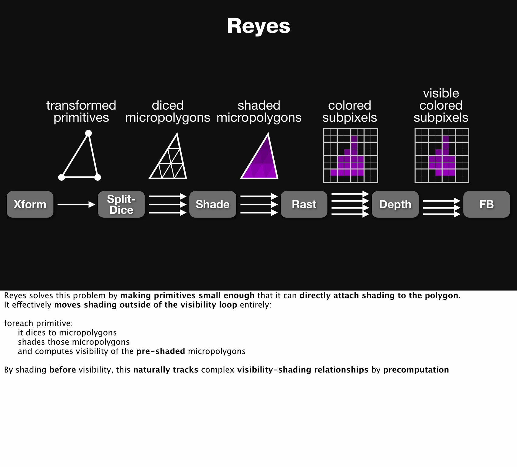
Reyes solves this problem by making primitives small enough that it can directly attach shading to the polygon.It effectively moves shading outside of the visibility loop entirely:
foreach primitive: it dices to micropolygons shades those micropolygons and computes visibility of the pre-shaded micropolygons
By shading before visibility, this naturally tracks complex visibility-shading relationships by precomputation

Reyes generalizes to blur
Xform Split-Dice Shade Rast Depth
transformedprimitives
FB
dicedmicropolygons
shadedmicropolygons
coloredsubpixels
visiblecolored
subpixels
Especially with blur, the relationship between micropolygons and the visibility samples they touch gets complex—these splats they cover in the framebuffer are strange and unpredictable shapes.
But Reyes naturally supports blur. The micropolygons can be stochastically rasterized just like any others.And since they were shaded ahead of time, it doesn't matter how blurry it gets, we only shade it once.
But we had to shade the micropolygon before knowing whether it was visible, violating our third rule: only shade points we can actually see.
Stochastic visibility sampling ✓ ✗ ✓
✗ ✓ ✓✓ ✓ ✗
Super-sampling MSAA Reyes
Shade at independent (lower)
frequency
Shade only what’s visible
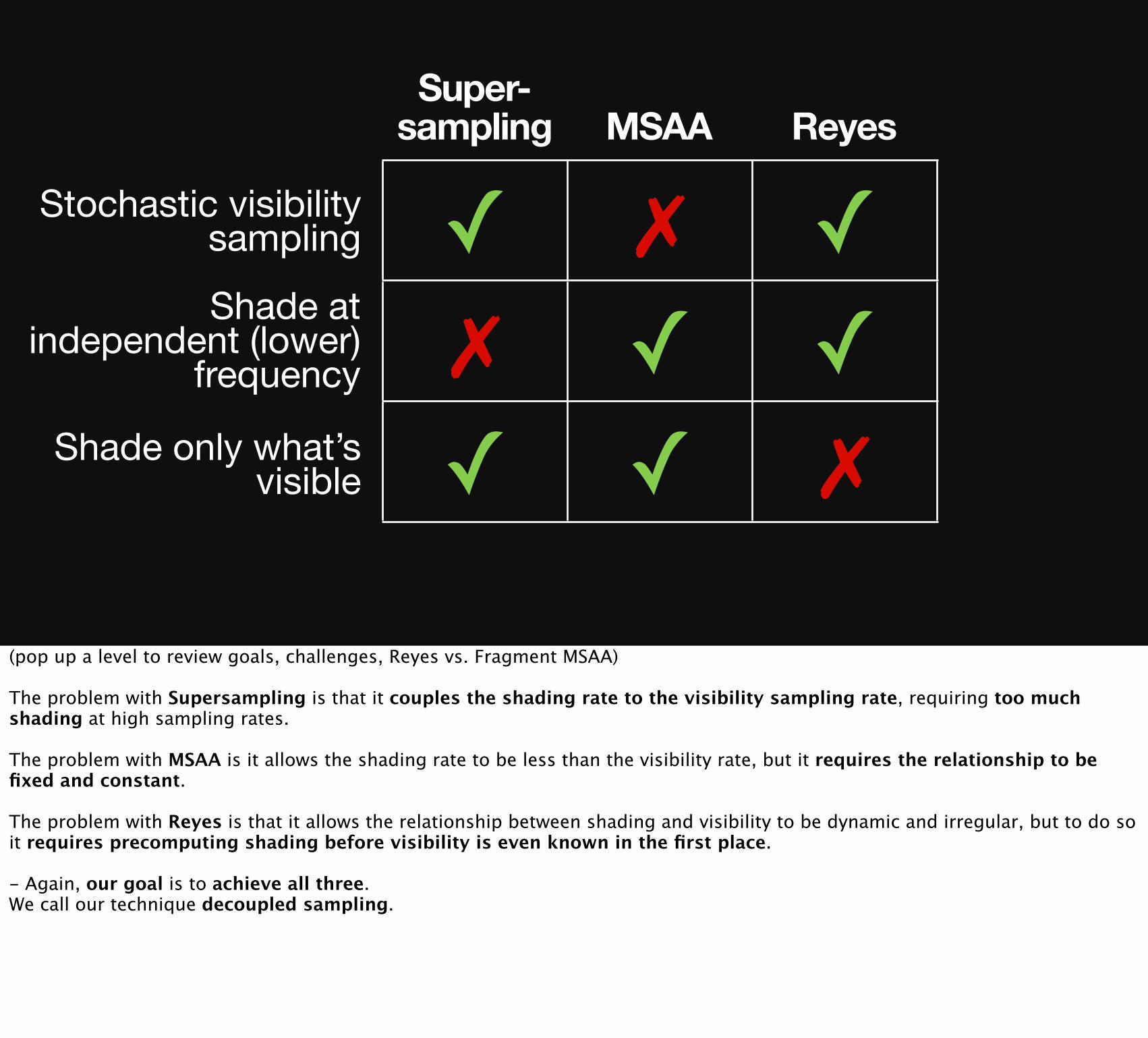
(pop up a level to review goals, challenges, Reyes vs. Fragment MSAA)
The problem with Supersampling is that it couples the shading rate to the visibility sampling rate, requiring too much shading at high sampling rates.
The problem with MSAA is it allows the shading rate to be less than the visibility rate, but it requires the relationship to be fixed and constant.
The problem with Reyes is that it allows the relationship between shading and visibility to be dynamic and irregular, but to do so it requires precomputing shading before visibility is even known in the first place.
- Again, our goal is to achieve all three.We call our technique decoupled sampling.

Stochastic visibility sampling ✓ ✗ ✓
✗ ✓ ✓✓ ✓ ✗
Super-sampling MSAA Reyes
Shade at independent (lower)
frequency
Shade only what’s visible
DecoupledSampling
✓✓✓
(pop up a level to review goals, challenges, Reyes vs. Fragment MSAA)
The problem with Supersampling is that it couples the shading rate to the visibility sampling rate, requiring too much shading at high sampling rates.
The problem with MSAA is it allows the shading rate to be less than the visibility rate, but it requires the relationship to be fixed and constant.
The problem with Reyes is that it allows the relationship between shading and visibility to be dynamic and irregular, but to do so it requires precomputing shading before visibility is even known in the first place.
- Again, our goal is to achieve all three.We call our technique decoupled sampling.

Our technique:Post-visibility Decoupled Sampling
1. Separate visibility from shading samples.
2. Define an explicit mapping from visibility to shading space.
3. Use a cache to manage irregular shading-visibility relationships, without precomputation.
Decoupled Sampling is built from three key ideas.
First, we modify the pipeline to explicitly separate visibility and shading samples.
Second, we define a consistent mapping from visibility samples to shading samples, which we use explicitly.
Finally, we use a simple cache to manage the dynamic, irregular relationship between shading and visibility samples under this mapping,rather than precomputing shading like Reyes.
foreach primitive:foreach vis sample:
skip if not visiblemap to shading sampleif not in cache:
shade and cacheelse:
use cached valuevisibility samples(screen space)
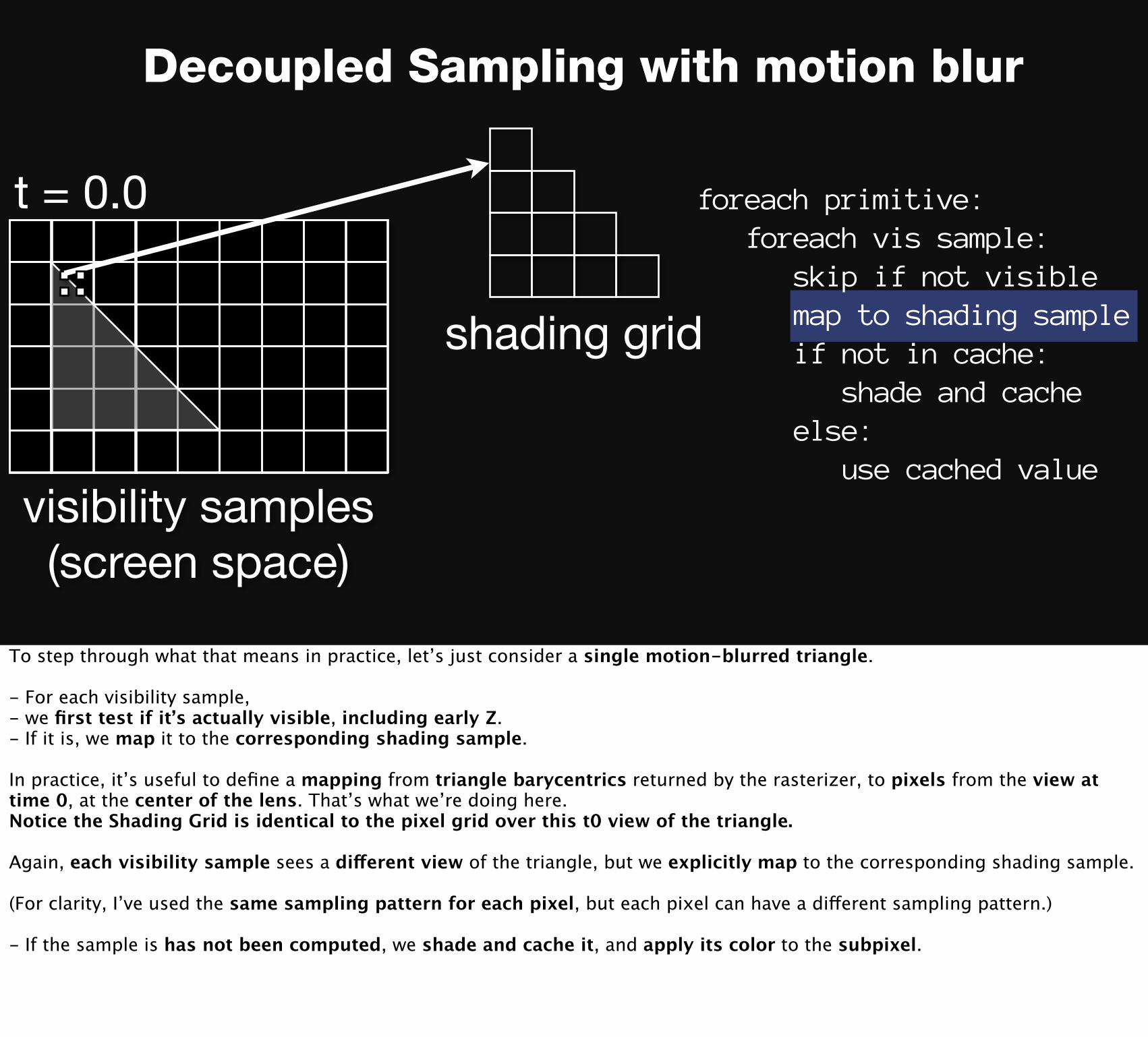
Decoupled Sampling with motion blur
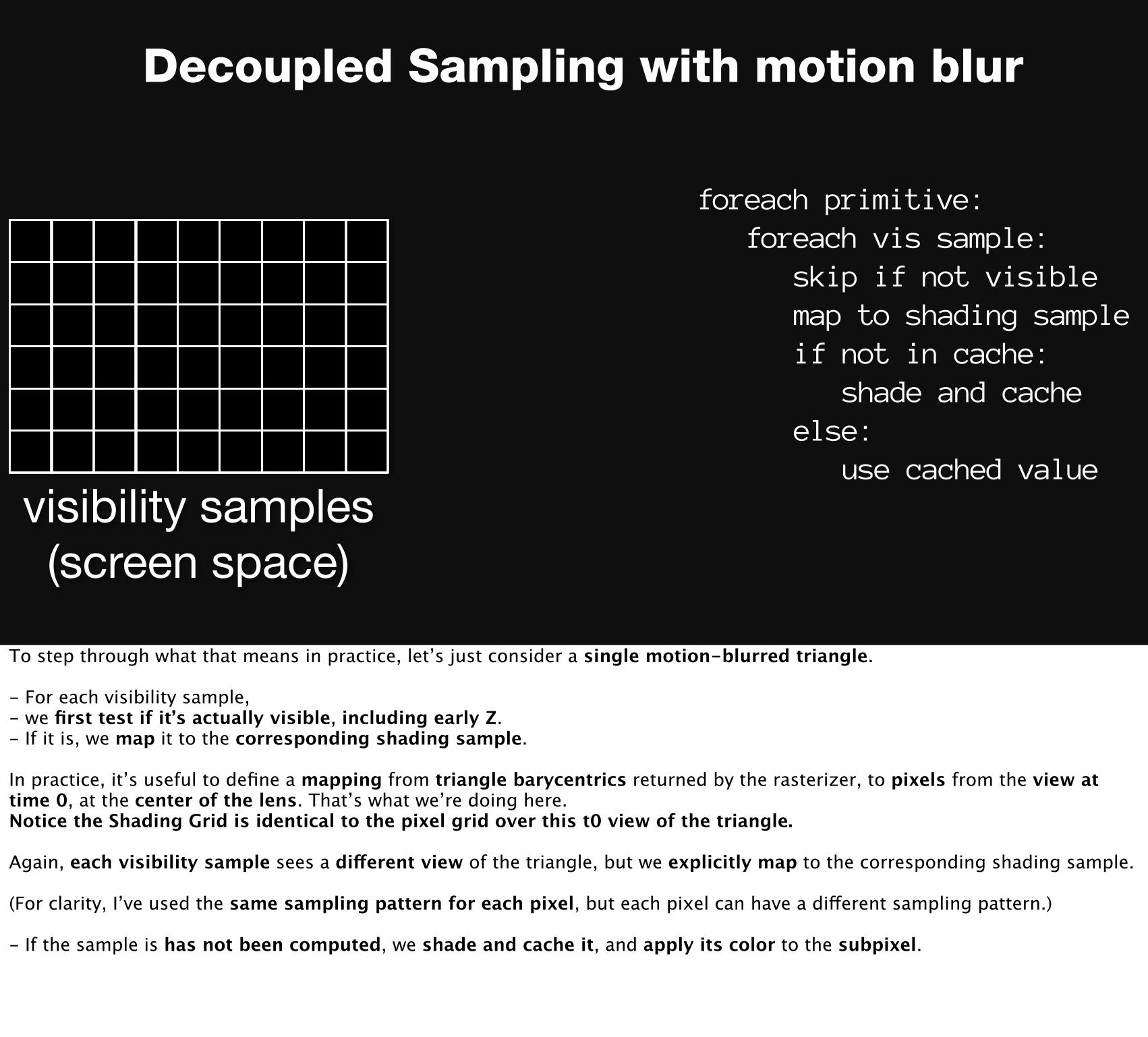
To step through what that means in practice, let’s just consider a single motion-blurred triangle.
- For each visibility sample,- we first test if it’s actually visible, including early Z.- If it is, we map it to the corresponding shading sample.
In practice, it’s useful to define a mapping from triangle barycentrics returned by the rasterizer, to pixels from the view at time 0, at the center of the lens. That’s what we’re doing here.Notice the Shading Grid is identical to the pixel grid over this t0 view of the triangle.
Again, each visibility sample sees a different view of the triangle, but we explicitly map to the corresponding shading sample.
(For clarity, I’ve used the same sampling pattern for each pixel, but each pixel can have a different sampling pattern.)
- If the sample is has not been computed, we shade and cache it, and apply its color to the subpixel.

foreach primitive:foreach vis sample:
skip if not visiblemap to shading sampleif not in cache:
shade and cacheelse:
use cached valuevisibility samples(screen space)
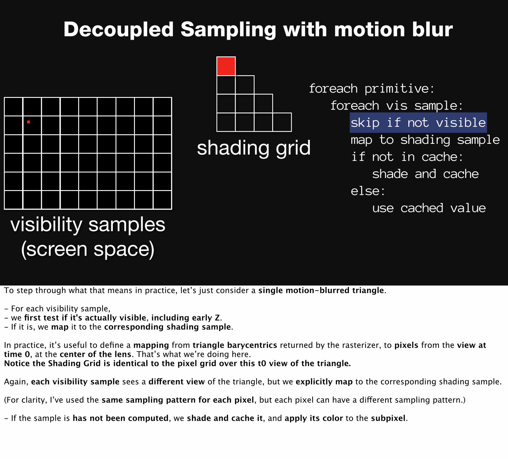
Decoupled Sampling with motion blur
To step through what that means in practice, let’s just consider a single motion-blurred triangle.
- For each visibility sample,- we first test if it’s actually visible, including early Z.- If it is, we map it to the corresponding shading sample.
In practice, it’s useful to define a mapping from triangle barycentrics returned by the rasterizer, to pixels from the view at time 0, at the center of the lens. That’s what we’re doing here.Notice the Shading Grid is identical to the pixel grid over this t0 view of the triangle.
Again, each visibility sample sees a different view of the triangle, but we explicitly map to the corresponding shading sample.
(For clarity, I’ve used the same sampling pattern for each pixel, but each pixel can have a different sampling pattern.)
- If the sample is has not been computed, we shade and cache it, and apply its color to the subpixel.

t = 0.0 foreach primitive:foreach vis sample:
skip if not visiblemap to shading sampleif not in cache:
shade and cacheelse:
use cached valuevisibility samples(screen space)
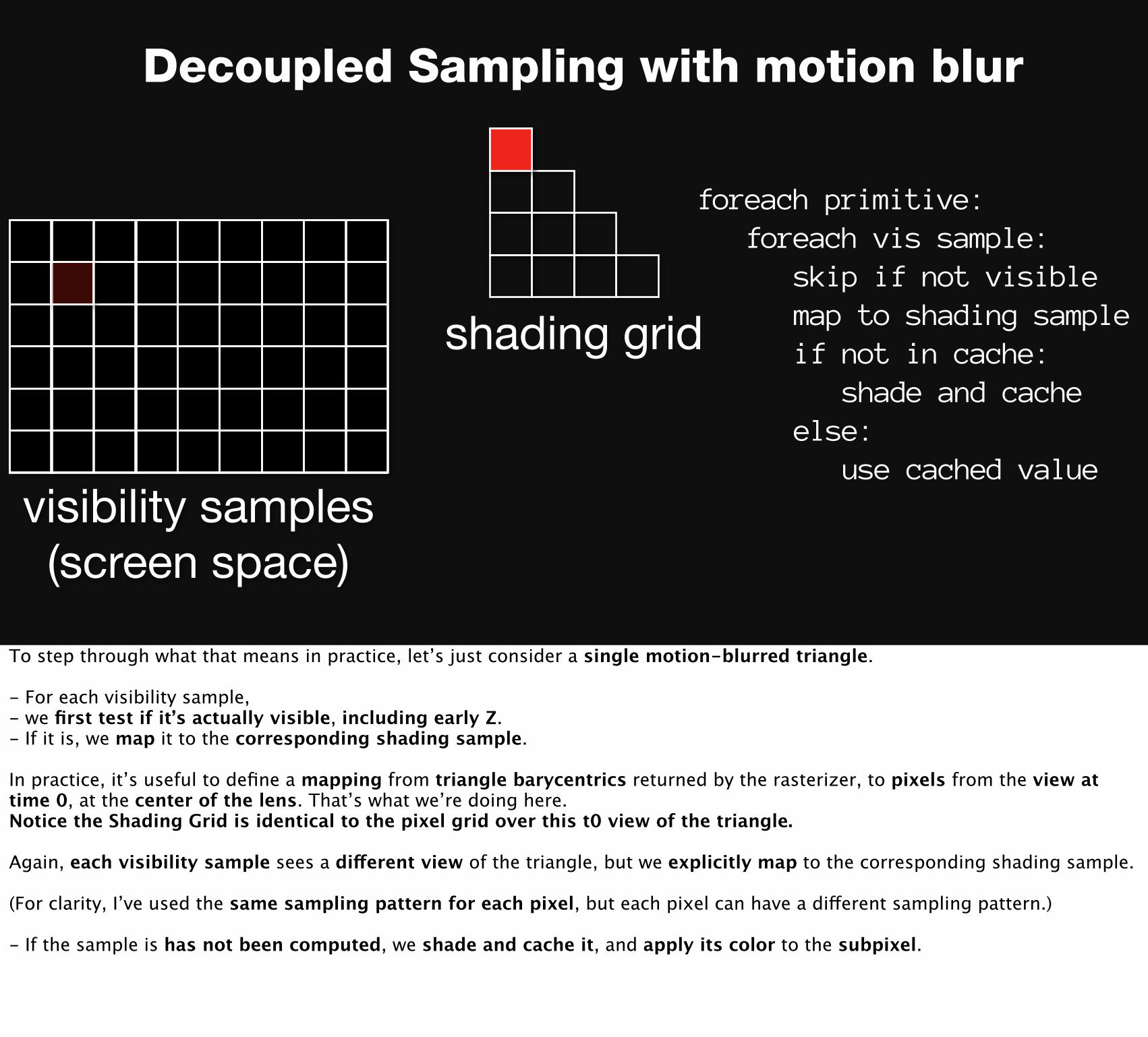
Decoupled Sampling with motion blur
To step through what that means in practice, let’s just consider a single motion-blurred triangle.
- For each visibility sample,- we first test if it’s actually visible, including early Z.- If it is, we map it to the corresponding shading sample.
In practice, it’s useful to define a mapping from triangle barycentrics returned by the rasterizer, to pixels from the view at time 0, at the center of the lens. That’s what we’re doing here.Notice the Shading Grid is identical to the pixel grid over this t0 view of the triangle.
Again, each visibility sample sees a different view of the triangle, but we explicitly map to the corresponding shading sample.
(For clarity, I’ve used the same sampling pattern for each pixel, but each pixel can have a different sampling pattern.)
- If the sample is has not been computed, we shade and cache it, and apply its color to the subpixel.

t = 0.0 foreach primitive:foreach vis sample:
skip if not visiblemap to shading sampleif not in cache:
shade and cacheelse:
use cached valuevisibility samples(screen space)
Decoupled Sampling with motion blur
To step through what that means in practice, let’s just consider a single motion-blurred triangle.
- For each visibility sample,- we first test if it’s actually visible, including early Z.- If it is, we map it to the corresponding shading sample.
In practice, it’s useful to define a mapping from triangle barycentrics returned by the rasterizer, to pixels from the view at time 0, at the center of the lens. That’s what we’re doing here.Notice the Shading Grid is identical to the pixel grid over this t0 view of the triangle.
Again, each visibility sample sees a different view of the triangle, but we explicitly map to the corresponding shading sample.
(For clarity, I’ve used the same sampling pattern for each pixel, but each pixel can have a different sampling pattern.)
- If the sample is has not been computed, we shade and cache it, and apply its color to the subpixel.
shading grid
t = 0.0 foreach primitive:foreach vis sample:
skip if not visiblemap to shading sampleif not in cache:
shade and cacheelse:
use cached valuevisibility samples(screen space)
Decoupled Sampling with motion blur
To step through what that means in practice, let’s just consider a single motion-blurred triangle.
- For each visibility sample,- we first test if it’s actually visible, including early Z.- If it is, we map it to the corresponding shading sample.
In practice, it’s useful to define a mapping from triangle barycentrics returned by the rasterizer, to pixels from the view at time 0, at the center of the lens. That’s what we’re doing here.Notice the Shading Grid is identical to the pixel grid over this t0 view of the triangle.
Again, each visibility sample sees a different view of the triangle, but we explicitly map to the corresponding shading sample.
(For clarity, I’ve used the same sampling pattern for each pixel, but each pixel can have a different sampling pattern.)
- If the sample is has not been computed, we shade and cache it, and apply its color to the subpixel.
shading grid
foreach primitive:foreach vis sample:
skip if not visiblemap to shading sampleif not in cache:
shade and cacheelse:
use cached valuevisibility samples(screen space)
Decoupled Sampling with motion blur
To step through what that means in practice, let’s just consider a single motion-blurred triangle.
- For each visibility sample,- we first test if it’s actually visible, including early Z.- If it is, we map it to the corresponding shading sample.
In practice, it’s useful to define a mapping from triangle barycentrics returned by the rasterizer, to pixels from the view at time 0, at the center of the lens. That’s what we’re doing here.Notice the Shading Grid is identical to the pixel grid over this t0 view of the triangle.
Again, each visibility sample sees a different view of the triangle, but we explicitly map to the corresponding shading sample.
(For clarity, I’ve used the same sampling pattern for each pixel, but each pixel can have a different sampling pattern.)
- If the sample is has not been computed, we shade and cache it, and apply its color to the subpixel.

shading grid
t = 0.0
visibility samples(screen space)
foreach primitive:foreach vis sample:
skip if not visiblemap to shading sampleif not in cache:
shade and cacheelse:
use cached value
Decoupled Sampling with motion blur
2nd actually misses, because of the regular spacing of the samples we’re using

shading grid
t = 0.75
visibility samples(screen space)
foreach primitive:foreach vis sample:
skip if not visiblemap to shading sampleif not in cache:
shade and cacheelse:
use cached value
Decoupled Sampling with motion blur
2nd actually misses, because of the regular spacing of the samples we’re using

shading grid
t = 0.0
visibility samples(screen space)
foreach primitive:foreach vis sample:
skip if not visiblemap to shading sampleif not in cache:
shade and cacheelse:
use cached value
Decoupled Sampling with motion blur
In the 3rd pixel, the 3rd visibility sample hits the top of the triangle.
Mapping to the shading grid, this part of the triangle has already been shaded,so we can reuse its value.

shading grid
t = 0.5
visibility samples(screen space)
foreach primitive:foreach vis sample:
skip if not visiblemap to shading sampleif not in cache:
shade and cacheelse:
use cached value
Decoupled Sampling with motion blur
In the 3rd pixel, the 3rd visibility sample hits the top of the triangle.
Mapping to the shading grid, this part of the triangle has already been shaded,so we can reuse its value.

shading grid
t = 0.75
visibility samples(screen space)
foreach primitive:foreach vis sample:
skip if not visiblemap to shading sampleif not in cache:
shade and cacheelse:
use cached value
Decoupled Sampling with motion blur
In the 3rd pixel, the 3rd visibility sample hits the top of the triangle.
Mapping to the shading grid, this part of the triangle has already been shaded,so we can reuse its value.

shading grid
t = …
visibility samples(screen space)
foreach primitive:foreach vis sample:
skip if not visiblemap to shading sampleif not in cache:
shade and cacheelse:
use cached value
Decoupled Sampling with motion blur
We render the rest of the triangle similarly.

shading grid
t = 0.0
visibility samples(screen space)
foreach primitive:foreach vis sample:
skip if not visiblemap to shading sampleif not in cache:
shade and cacheelse:
use cached value
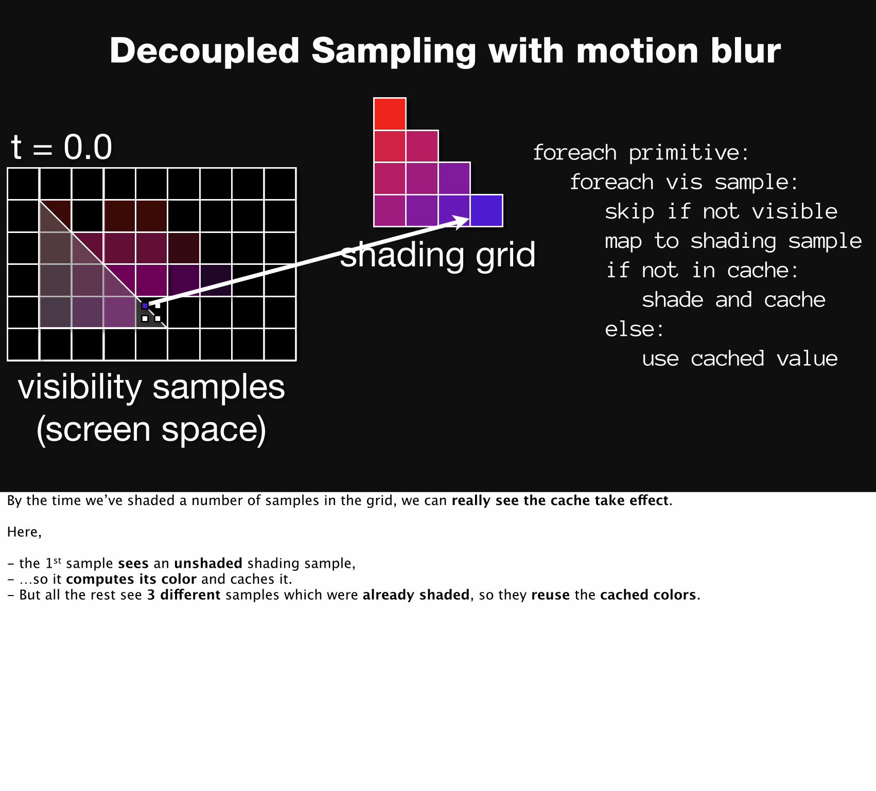
Decoupled Sampling with motion blur
By the time we’ve shaded a number of samples in the grid, we can really see the cache take effect.
Here,
- the 1st sample sees an unshaded shading sample,- …so it computes its color and caches it.- But all the rest see 3 different samples which were already shaded, so they reuse the cached colors.

shading grid
t = 0.0
visibility samples(screen space)
foreach primitive:foreach vis sample:
skip if not visiblemap to shading sampleif not in cache:
shade and cacheelse:
use cached value
Decoupled Sampling with motion blur
By the time we’ve shaded a number of samples in the grid, we can really see the cache take effect.
Here,
- the 1st sample sees an unshaded shading sample,- …so it computes its color and caches it.- But all the rest see 3 different samples which were already shaded, so they reuse the cached colors.

shading grid
t = 0.75
visibility samples(screen space)
foreach primitive:foreach vis sample:
skip if not visiblemap to shading sampleif not in cache:
shade and cacheelse:
use cached value
Decoupled Sampling with motion blur
By the time we’ve shaded a number of samples in the grid, we can really see the cache take effect.
Here,
- the 1st sample sees an unshaded shading sample,- …so it computes its color and caches it.- But all the rest see 3 different samples which were already shaded, so they reuse the cached colors.

shading grid
visibility samples(screen space)
foreach primitive:foreach vis sample:
skip if not visiblemap to shading sampleif not in cache:
shade and cacheelse:
use cached value
Decoupled Sampling with motion blur
By the end,we’ve sampled visibility 4x per pixel to capture motion blur,but we’ve only shaded approximately once per pixel.
…to pop up to how that looks in an actual pipeline…

Decoupled Sampling
Xform Rast Depth-Stencil Map FB
transformedprimitives
coveredsubpixels
visiblesubpixels
Cache
Shade
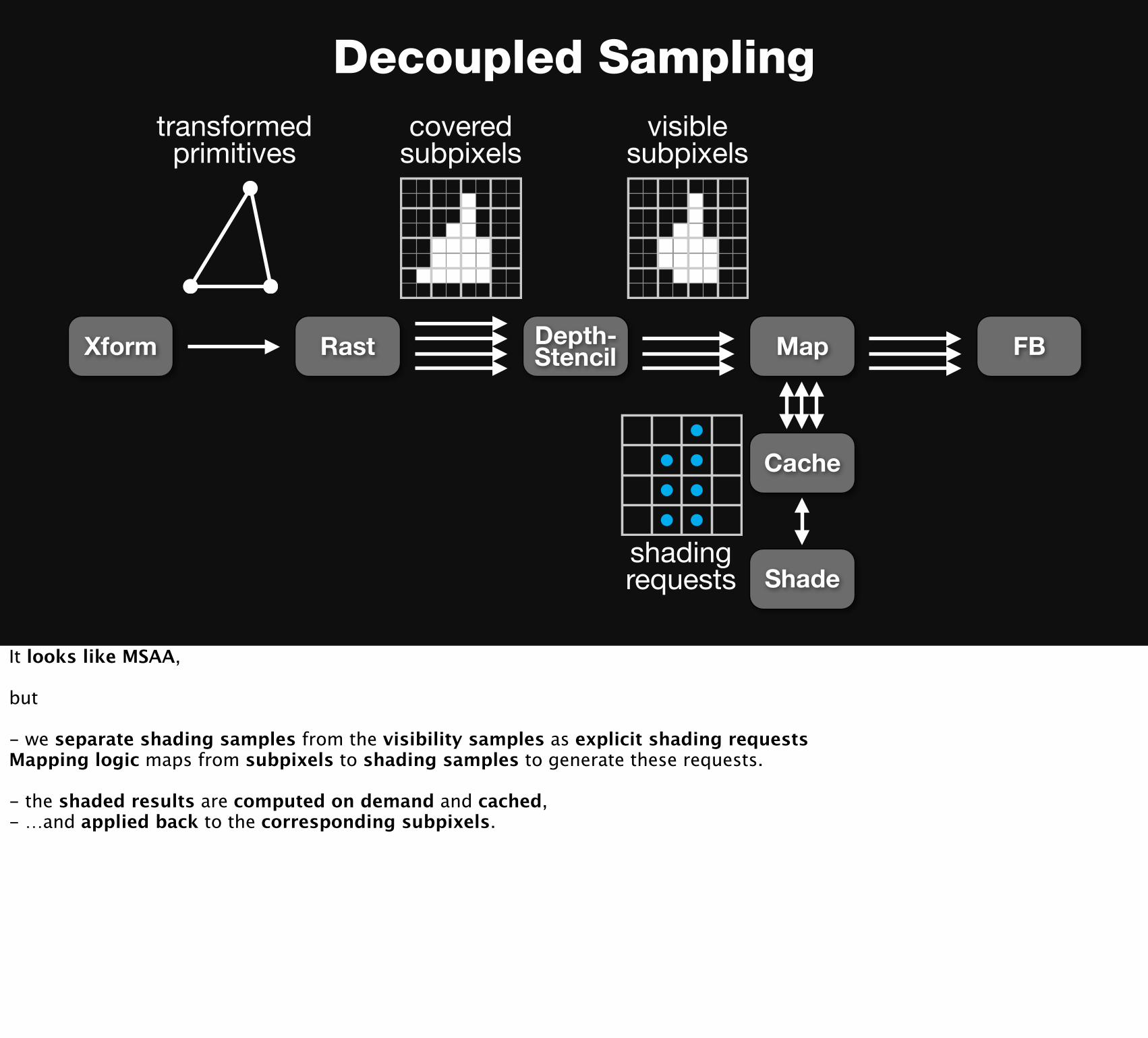
It looks like MSAA,
but
- we separate shading samples from the visibility samples as explicit shading requestsMapping logic maps from subpixels to shading samples to generate these requests.
- the shaded results are computed on demand and cached,- …and applied back to the corresponding subpixels.
Decoupled Sampling
Xform Rast Depth-Stencil Map FB
transformedprimitives
coveredsubpixels
visiblesubpixels
shadingrequests
Cache
Shade
It looks like MSAA,
but
- we separate shading samples from the visibility samples as explicit shading requestsMapping logic maps from subpixels to shading samples to generate these requests.
- the shaded results are computed on demand and cached,- …and applied back to the corresponding subpixels.

Decoupled Sampling
Xform Rast Depth-Stencil Map FB
transformedprimitives
coveredsubpixels
visiblesubpixels
shadingrequests
Cache
Shadeshadedresults
It looks like MSAA,
but
- we separate shading samples from the visibility samples as explicit shading requestsMapping logic maps from subpixels to shading samples to generate these requests.
- the shaded results are computed on demand and cached,- …and applied back to the corresponding subpixels.

Decoupled Sampling
Xform Rast Depth-Stencil Map FB
transformedprimitives
coveredsubpixels
visiblesubpixels
coloredsubpixels
shadingrequests
Cache
Shadeshadedresults
It looks like MSAA,
but
- we separate shading samples from the visibility samples as explicit shading requestsMapping logic maps from subpixels to shading samples to generate these requests.
- the shaded results are computed on demand and cached,- …and applied back to the corresponding subpixels.
Decoupled Sampling
Xform Rast Depth-Stencil Map FB
transformedprimitives
coveredsubpixels
visiblesubpixels
coloredsubpixels
shadingrequests
Cache
Shadeshadedresults
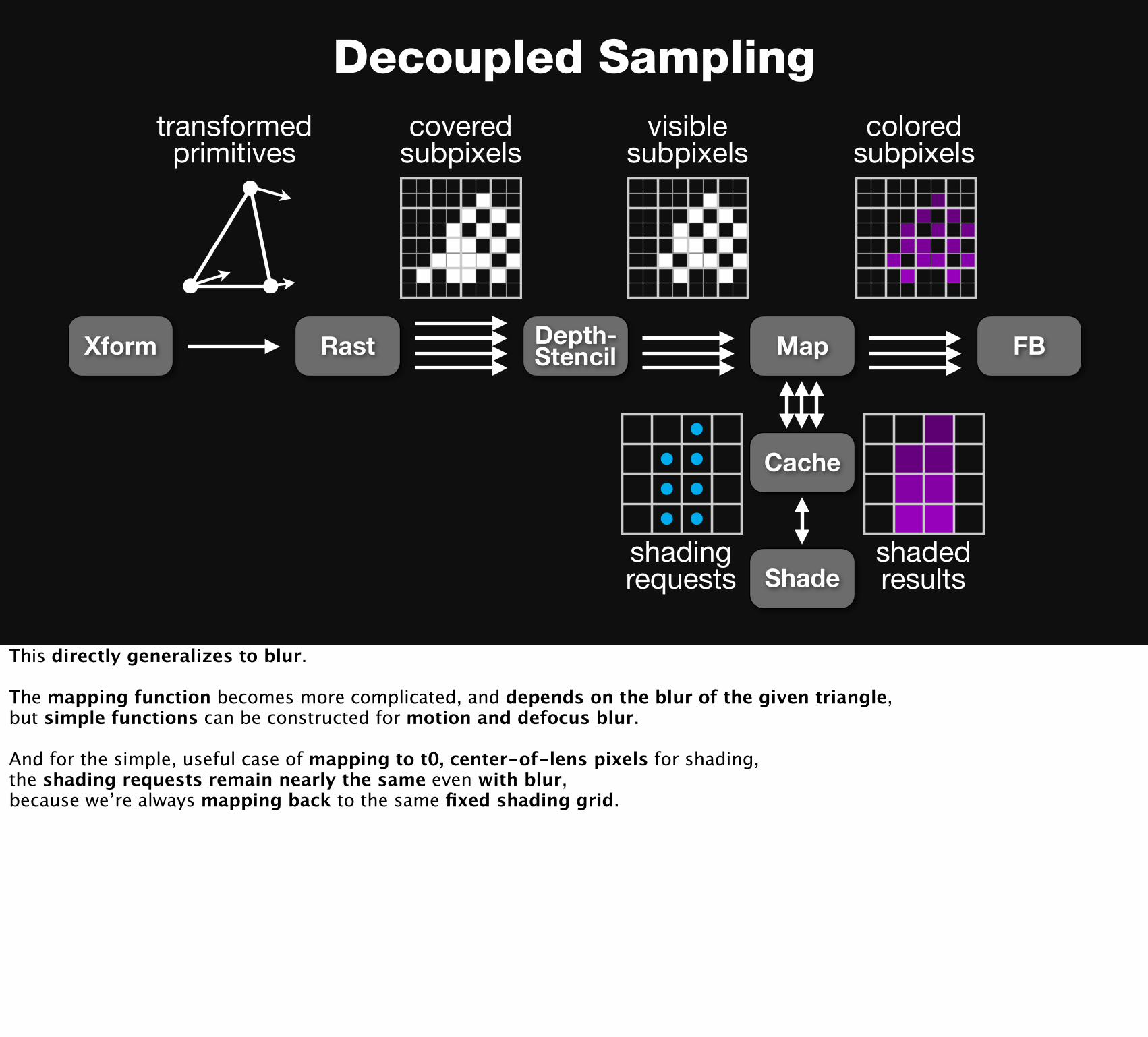
This directly generalizes to blur.
The mapping function becomes more complicated, and depends on the blur of the given triangle,but simple functions can be constructed for motion and defocus blur.
And for the simple, useful case of mapping to t0, center-of-lens pixels for shading,the shading requests remain nearly the same even with blur,because we’re always mapping back to the same fixed shading grid.

Results
So, how does it work…

0
1
2
3
4
5
Sort Last
●●●● ● ● ● ● ● ● ● ● ●
●●● ● ● ● ● ● ● ● ● ● ●
●●● ● ● ● ● ● ● ● ● ● ●
0 50 100 150 200 250
Tiled
●●● ●
● ● ● ● ● ● ● ●●
●
●●●
●●
●●
●
●●
●
●
●
●●●
●●
●
●
●
●
●
●
●
0 50 100 150 200 250
shad
ing
rate
64 samples/pixel27 samples/pixel8 samples/pixel
blur area (pixels)
Blur vs. shading rate: defocusmoderateblur
no blur heavyblur
Half-Life 2, Episode 21280x720, 27 samples/pixel
4.5-43x less shading than ideal supersampling
Well.
We implemented decoupled sampling in an instrumented D3D9 simulator, and tested it with real content.
On this frame from Half-Life 2, Episode 2, with at 27 visibility samples per pixel,an average defocus blur of 1- to 200 pixels in area shades under 1.7 samples per pixel on average, vs. 27 for idealized supersampling.
The graph shows how many times we shade per covered pixel, on the Y-axis,as a function of blur area, on the X-axis.The different colored lines are different sampling rates.
The shading rate per covered pixel only grows minimally with sampling rate and blur,where it would be a much higher constant rate equal to the visibility sampling rate for supersampling.

Blur vs. shading rate: motion
shad
ing
rate
blur area (pixels)
0
5
10
15
Sort Last
● ● ● ● ● ● ● ● ● ●
● ● ● ● ● ●●
●●
●
● ● ● ●●
●●
●●
●
0 20 40 60 80 100 120
Tiled
●●
●●
●●
●
●
●●
●
●●
●
●
●
●
●
●
●
●
●
●
●
●
●
●
●
●
●
0 20 40 60 80 100 120
64 samples/pixel27 samples/pixel8 samples/pixel
moderateblur
noblur
heavyblur
Team Fortress 21280x720, 27 samples/pixel
3-40x less shading than ideal supersampling
similarly for this frame from Team Fortress 2, with lots of motion blur from a spinning camera.
The shading rate grows weakly in blur size or sampling rate.
But it does grow somewhat more at extreme blur here, because shading samples on some triangles spread much farther apartalong the screen-space Moreton curve rasterization order which generates the shading requests.
But in all cases it shades many times less than supersampling.
These results are all for a single 1k quad decoupling cache, which would fit into 16-32 kilobytes,but we’ve also studied effectiveness as a function of cache size, and this small cache nearly always comes quite close to optimal.

Blur vs. Shading Rate
blu
r ar
ea (p
ixel
s)sh
adin
g ra
te
0
1
2
3
4Sort Last
0 10 20 30 40 500
10
20
30
40
50
Tiled
0 10 20 30 40 50
frame
1000
2000
3000
4000
5000
6000
7000
0 10 20 30 40 50
64 samples/pixel27 samples/pixel8 samples/pixel
In this scene with both motion and defocus blur,while the amount of blur, shown on the bottom, varies widely over the animation,the shading rate still remains relatively constant.
(pause)The one thing to note is that it is 2x higher than the game frames.That’s because this scene has many tiny triangles, and quad occupancy reduces efficiency.
Point out: decoupling is a natural fit for a fragment merging-type idea—we could define shading space as spanning the surface, rather than just within the bounds of the triangle.

Decoupled Sampling:
✓ Scales to large numbers of stochastic visibility samples.
✓ Shades at the lowest frequency possible.
✓ Only shades visible points.
Back to our design goals,these results show decoupled sampling scaling to high stochastic sampling rates with blur,while shading at a low, controlled rate of little over once per pixel.
And since shading is only computed after precise visibility,it only shades visible points, which actually contribute to the final image.
(pop up)It’s also worth realizing thatthis mapping is more general than just screen-space shading for motion blur and depth of field.

We can map to more than t0 pixels:blur-adaptive shading rate
Adaptive shading rate:37% less shading
max pixel error <5%
5%
0%
…as one exampleif we know that a certain triangle is going to be blurry,we can shade even less than once per pixel.
-------------------- SKIP FOR TIME --------------------Here, we’ve defined the shading sample frequency to reduce as a function of defocus blur.This gives an effectively identical image while shading almost 40% less overall.

We could map to object-space
Burns et al. 2010A Lazy Object-Space Shading Architecture with Decoupled Sampling.
We could also define our mapping to some desired shading rate in object space.And in effect, this is what Chris Burns, Kayvon, and Bill Mark presented at HPG this year, which is another great paper to check out.
-------------------- SKIP --------------------Integrated with a Reyes-style renderer, this gives them the flexibility to dice to potentially _larger_ than subpixel triangles (since it decouples shading rate from and it shades _after_ precise visibility, reducing overshade.
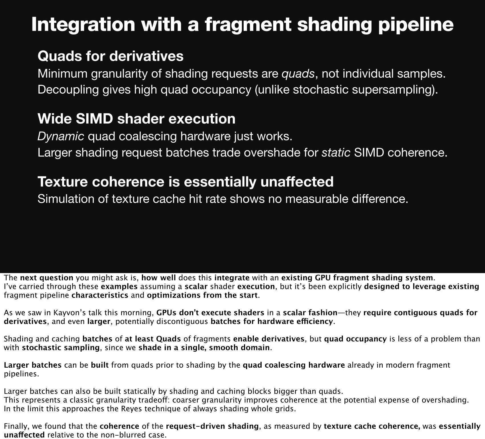
Integration with a fragment shading pipeline
Quads for derivativesMinimum granularity of shading requests are quads, not individual samples.Decoupling gives high quad occupancy (unlike stochastic supersampling).
Wide SIMD shader executionDynamic quad coalescing hardware just works.Larger shading request batches trade overshade for static SIMD coherence.
Texture coherence is essentially unaffectedSimulation of texture cache hit rate shows no measurable difference.
The next question you might ask is, how well does this integrate with an existing GPU fragment shading system.I’ve carried through these examples assuming a scalar shader execution, but it’s been explicitly designed to leverage existing fragment pipeline characteristics and optimizations from the start.
As we saw in Kayvon’s talk this morning, GPUs don’t execute shaders in a scalar fashion—they require contiguous quads for derivatives, and even larger, potentially discontiguous batches for hardware efficiency.
Shading and caching batches of at least Quads of fragments enable derivatives, but quad occupancy is less of a problem than with stochastic sampling, since we shade in a single, smooth domain.
Larger batches can be built from quads prior to shading by the quad coalescing hardware already in modern fragment pipelines.
Larger batches can also be built statically by shading and caching blocks bigger than quads.This represents a classic granularity tradeoff: coarser granularity improves coherence at the potential expense of overshading.In the limit this approaches the Reyes technique of always shading whole grids.
Finally, we found that the coherence of the request-driven shading, as measured by texture cache coherence, was essentially unaffected relative to the non-blurred case.

Summary
It is possible to decouple shading from visibility samplingin a fragment shading system.Explicit mapping from shading to visibility samples decouples rates.Caching naturally manages irregular communication.
Decoupled Sampling makes GPU-style pipelines scalable to rendering with stochastic blur at modest shading cost.
Stochastic motion and defocus blur are becoming feasible for GPUs!
So in summary,It is possible to fully decouple shading from visibility sampling in a fragment shading system, with precise visibility.
We can do this by explicitly separating shading from visibility sampling,defining an explicitly-computed mapping from visibility to shading samples,and using a small cache to dynamically manage the resulting irregular communication.
By decoupling shading from visibility rates, Decoupled Sampling makes GPU-style pipelines scalable to rendering with stochastic blur without prohibitive shading cost.
Coupled with all the recent work in stochastic visibility for real-time systems,and additional simulation in our paper on the efficiency of ROP caches with blur,the reduced shading cost allowed by decoupled sampling makes stochastic motion and defocus blur really start to look feasible for real-time performance on GPUs.

Thank you
Special thanks: Jason Mitchell - Valve content NVIDIA, Intel, Singapore-MIT Gambit - Funding Kayvon Fatahalian, Jeremy Sugerman, Solomon Boulos - Talk feedback