Embed Size (px)
Citation preview

doi:10.1006/jsco.2000.0402Available online at http://www.idealibrary.com on
J. Symbolic Computation (2001) 31, 367–408
Decomposition Plans for Geometric ConstraintSystems, Part I: Performance Measures for CAD
CHRISTOPH M. HOFFMAN†§, ANDREW LOMONOSOV‡¶
AND MEERA SITHARAM‡¶‖
†Computer Science, Purdue University, West Lafayette, IN 47907, U.S.A.‡CISE, University of Florida, Gainesville, FL 32611-6120, U.S.A.
A central issue in dealing with geometric constraint systems for CAD/CAM/CAE is thegeneration of an optimal decomposition plan that not only aids efficient solution, but also
captures design intent and supports conceptual design. Though complex, this issue has
evolved and crystallized over the past few years, permitting us to take the next importantstep: in this paper, we formalize, motivate and explain the decomposition–recombination(DR)-planning problem as well as several performance measures by which DR-planningalgorithms can be analyzed and compared. These measures include: generality, valid-
ity, completeness, Church–Rosser property, complexity, best- and worst-choice approx-imation factors, (strict) solvability preservation, ability to deal with underconstrainedsystems, and ability to incorporate conceptual design decompositions specified by thedesigner. The problem and several of the performance measures are formally defined herefor the first time—they closely reflect specific requirements of CAD/CAM applications.
The clear formulation of the problem and performance measures allow us to precisely
analyze and compare existing DR-planners that use two well-known types of decom-position methods: SR (constraint shape recognition) and MM (generalized maximum
matching) on constraint graphs. This analysis additionally serves to illustrate and pro-vide intuitive substance to the newly formalized measures.
In Part II of this article, we use the new performance measures to guide the develop-ment of a new DR-planning algorithm which excels with respect to these performancemeasures.
c© 2001 Academic Press
1. Introduction and Motivation
Geometric constraints are at the heart of computer aided engineering applications (see,e.g. Hoffmann and Rossignac, 1996; Hoffmann, 1997), and also arise in many geometricmodeling contexts such as virtual reality, robotics, molecular modeling, teaching geom-etry, etc. Both parts of this paper, however, deal with geometric constraint systemsprimarily within the context of product design and assembly. Figure 3 illustrates those(boldface) components within a standard CAD/CAM/CAE master model architecture(Bronsvoort and Jansen, 1994; Kraker et al., 1997; Hoffmann and Joan-Arinyo, 1998)that Parts I and II of this paper directly address.
§Supported in part by NSF Grants CDA 92-23502 and CCR 95-05745, and by ONR Contract N00014-96-1-0635.¶Supported in part by NSF Grant CCR 94-09809.‖Corresponding Author: E-mail: [email protected]
0747–7171/01/040367 + 42 $35.00/0 c© 2001 Academic Press

368 C. M. Hoffman et al.
Note. Throughout this manuscript, slant is used for emphasis, while italics are used forintroducing new terminology.
Informally, a geometric constraint problem consists of a finite set of geometric objectsand a finite set of constraints between them. The geometric objects are drawn from a fixedset of types such as points, lines, circles and conics in the plane, or points, lines, planes,cylinders and spheres in three dimensions. The constraints are spatial and include logicalconstraints such as incidence, tangency, perpendicularity, etc., and metric constraintssuch as distance, angle, radius, etc. The spatial constraints can usually be written asalgebraic equations whose variables are the coordinates of the participating geometricobjects.
A solution of a geometric constraint problem is a real zero of the corresponding alge-braic system. In other words, a solution is a class of valid instantiations of the geometricelements such that all constraints are satisfied. Here, it is understood that such a solutionis in a particular geometry, for example the Euclidean plane, the sphere, or Euclideanthrree-dimensional space. For recent reviews of the extensive literature on geometricconstraint solving see, e.g. Hoffmann et al. (1998), Kramer (1992) and Fudos (1995).
1.1. the main reason to decompose geometric constraint systems
Currently there is a lack of effective spatial variational constraint solvers and assem-bly constraint solvers that scale to large problem sizes and can be used interactivelyby the designer as conceptual tools throughout the design process. Almost all currentCAD/CAM systems primarily use a non-variational, history-based three-dimensionalconstraint mechanism. This basic inadequacy in spatial constraint solving seriously hin-ders progress in the development of intelligent and agile CAD/CAM/CAE systems.
One governing issue is efficiency: computing the solution of the non-linear algebraicsystem that arises from geometric constraints is computationally challenging, and exceptfor very simple geometric constraint systems, this problem is not tractable in practicewithout further machinery. The so-called constraint propagation-based solvers (e.g. Gaoand Chou, 1998a; Klein, 1998) generally suffer from a drawback that cannot be easilyovercome: they find it difficult to decompose cyclically constrained systems, an essentialfeature of variational problems. Direct approaches to algebraically processing the entiresystem include:
(1) standard methods for polynomial ideal membership and locating solutions in alge-braically closed fields, for example using Grobner bases (Ruiz and Ferreira, 1996)or the Wu–Ritt method (Chou et al., 1996; Gao and Chou, 1998b);
(2) numerous algorithms and implementations for solving over the reals based on themethods of, for example, Canny (1993), Renegar (1992), Collins (1975) and Lazard(1981), etc.; and
(3) algorithms for decomposing and solving sparse polynomial systems based on Cannyand Emiris (1993), Sturmfels (1993), Khovanskii (1978), Sridhar et al. (1993) andSridhar et al. (1996), etc.
These direct algebraic solvers deal with general systems of polynomial equations, i.e.they do not exploit geometric domain knowledge; partly as a result, they have at leastexponential time complexity and they are slow in practice as well. In addition, they do not

Decomposition of Geometric Constraints I 369
take into account design considerations and as a result, cannot assist in the conceptualdesign process. These drawbacks apply to direct numerical solvers as well, including thosethat use homotopy continuation methods, see, for example, Durand (1998). The problemwould be further compounded if we allowed constraints that are natural in the designprocess, but which must be expressed as inequalities, such as “point P is to the leftof the oriented line L in the plane”. Such additions would necessitate using cylindricalalgebraic decomposition-based techniques (Collins, 1975), such as Grigor’ev and Vorobjov(1988), Lazard (1991) and Wang (1993) which have a theoretical worst-case complexityof O(2n
2), where n is the algebraic size of the problem; or alternatively require the use
of non-linear optimization techniques, all of which are slow enough in practice that theydo not represent a viable option for large problem sizes.
With regard to efficiency, the following rule of thumb has therefore emerged from yearsof experimentation with geometric, spatial constraint solvers in engineering design andassembly: the use of direct algebraic/numeric solvers for solving large subsystems rendersa geometric constraint solver practically useless (see Durand, 1998, for a natural exampleof a geometric constraint system with six primitive geometric objects and 15 constraints,which has repeatedly defied attempts at tractable solution). The overwhelming cost ingeometric constraint solving is directly proportional to the size of the largest subsystemthat is solved using a direct algebraic/numeric solver. This size dictates the practicalutility of the overall constraint solver, since the time complexity of the constraint solveris at least exponential in the size of the largest such subsystem.
Therefore, the constraint solver should use geometric domain knowledge to develop aplan for decomposing the constraint system into small subsystems, whose solutions canbe recombined by solving other small subsystems. The primary aim of this decompositionplan is to restrict the use of direct algebraic/numeric solvers to subsystems that are assmall as possible. Hence the optimal or most efficient decomposition plan would minimizethe size of the largest such subsystem. Any geometric constraint solver should first solvethe problem of efficiently finding a close-to-optimal decomposition–recombination (DR)plan, because that dictates the usability of the solver. Finding a DR-plan can be done asa pre-processing step by the constraint solver: a robust DR-plan would remain unchangedeven as minor changes to numerical parameters or other such on-line perturbations tothe constraint system are made during the design process.
In addition to optimality (efficiency), other equally important (and sometimes com-peting) issues arise from the fact that a DR-plan is a key conceptual component of theCAD model and should aid the overall design or assembly process. These issues will bediscussed under “Desirable characteristics” later in this section.
A clean and precise formulation of the DR-planning problem is therefore a fundamentalnecessity. To our knowledge, despite its longstanding presence, the DR-planning problemhas not yet been clearly isolated or precisely formulated, although there have been manyprior, specialized DR-planners that utilize geometric domain knowledge (e.g. Serranoand Gossard, 1986; Crippen and Havel, 1988; Serrano, 1990; Havel, 1991; Owen, 1991,1996; Kramer, 1992; Ait-Aoudia et al., 1993; Pabon, 1993; Hoffmann and Vermeer, 1994,1995; Bouma et al., 1995; Hsu, 1996; Fudos and Hoffmann, 1996b, 1997; Latham andMiddleditch, 1996). See Hoffmann et al. (1998) for an exposition of two primary classes ofexisting methods of decomposing geometric constraint systems; representative algorithmsfrom these two classes are extensively analyzed in Section 4. In Part II of this paper we

370 C. M. Hoffman et al.
describe and analyze a new algorithm that performs well with respect to the measuresdescribed below.
In the next two subsections we informally describe both the basic requirements of aDR-plan(ner) that dictate its overall structure, as well as desirable characteristics of theDR-plan(ner) that improve efficiency and assist in the design process.
1.2. basic requirements of a decomposition plan
Recall that a DR-plan specifies a plan for decomposing a constraint system into smallsubsystems and recombining solutions of these subsystems later. Therefore the first re-quirement of a DR-plan is that the solutions of the small subsystems in the decompositioncan be recombined into a solution of the entire system. In other words, it should be pos-sible to substitute the (set of) solution(s) of each subsystem into the entire system ina natural manner, resulting in a simpler system. Secondly, we would like these inter-mediate subsystems that are solved during the decomposition and recombination to begeometrically meaningful.
Together, these two requirements on the intermediate subsystems translate to a re-quirement that the subsystems be geometrically rigid. A rigid or solvable subsystem ofthe constraint system is one for which the set of real-zeroes of the corresponding algebraicequations is discrete (i.e. the corresponding real-algebraic variety is zero-dimensional),after the local coordinate system is fixed arbitrarily, i.e. after an appropriate numberof degrees of freedom D are fixed arbitrarily. The constant D is usually the number of(translational and rotational) degrees of freedom available to any rigid object in the givengeometry (three in two dimensions, six in three dimensions, etc.) and in some cases, D de-pends on other symmetries of the subsystem. An underconstrained system is not solvable,i.e. its set of real zeroes is not discrete (non-zero-dimensional). A well-constrained systemis a solvable system where removal of any constraint results in an underconstrained sys-tem. An overconstrained system is a solvable system in which there is a constraint whoseremoval still leaves the system solvable. Solvable systems of equations are therefore well-constrained or overconstrained. That is, the constraints force a finite number of isolatedreal solutions, so one solution cannot be obtained by an infinitesimal perturbation ofanother. For example, Figure 1 shows a solvable subsystem of three points and threedistances between pairs of points. A consistently overconstrained system is one whichhas at least one real zero.
Note. It is important to distinguish “solvable” from “has a real solution”. Although(inconsistently) overconstrained (or even certain well-constrained) systems may have noreal solutions at all, by our definition, since their set of real zeroes is discrete, they wouldstill be considered “solvable”. In general, whenever a subsystem of a constraint system isdetected that has no real solutions, then the solution process would have to immediatelyhalt and inform the designer of this fact.
Informally, a geometric constraint solver which solves a large constraint system E byusing a DR-planner—to guide a direct algebraic/numeric solver capable of solving smallsubsystems—proceeds by repeatedly applying the following three steps at each iteration i.
(1) Find a small solvable subsystem Si of the (current) entire system Ei (at the firstiteration, this is simply the given constraint system E, i.e. E1 = E). This step is

Decomposition of Geometric Constraints I 371
A B
C
D: (x1 — x2)2+ (y1 — y2)2—A2
E: (x2 — x3)2+ (y2 — y3)2—B2
P3
F: (x3 — x1)2 + (y3 — y1)2—C2
P1
P2
Figure 1. A solvable system of equations.
E E = T (E ) E = T (E ) E = T T (E )n –1 1 1 2 232 111
S T (S )
S
S
T (S )
T (T (S ))
S
1 1 1
2
3
2 2
2 1 1
n . . .
Figure 2. Solving a well-constrained system by decomposition: Step 1—rectangles, Step 3—ovals.
indicated by a rectangle in Figure 2. The subsystem Si could be also chosen by thedesigner.
(2) Solve Si using the direct algebraic/numeric solver.(3) Using the output of the solver, and perhaps using the designer’s help to eliminate
some solutions, replace Si by an abstraction or simplification Ti(Si) thereby replac-ing the entire system Ei by a simplification Ti(Ei) = Ei+1. This step is indicatedby an oval in Figure 2. Some informal requirements on the simplifiers Ti are thefollowing: we would like Ei to be (real algebraically) inferable from Ei+1; i.e. wewould like any real solution of Ei+1 to be a solution of Ei as well.
A constraint solver that fits the above structural description—which we shall refer toas S in future discussions—is called a decomposition–recombination (DR) solver. (Theformal definition imposes further requirements on simplifier Ti—see the next section.)This solver terminates when the small, solvable subsystem Si found in Step 1 is the entirepolynomial system Ei. An optimal DR-plan will minimize the size of the largest Si. Ifthe whole system is underconstrained, the solver should still solve its maximal solvablesubsystems.
For the purpose of planning a solution sequence a priori, we would like to executeSteps 1 and 3 alone without access to the algebraic solver, and obtain a DR-plan, withoutactually solving the subsystems. That is, i.e. we would like the constraint solver to lookas in Figure 3, with the DR-planner driving the direct algebraic/numeric solver.

372 C. M. Hoffman et al.
model
model
model
Masterconstraintmodel
Master
View/system
GD&Tplan
View/system
Other
downstreams
GD&T MPPmodel
MPP
model
constr.constr.
Master model server
GD&T
CAD
View/
system
Constraint solver
Constraint model manipulator
Decomp.
planner
Algebraic
solver
CAD model
Optional design history
of constraint models
(for non-variational case)
CADconstraint
model
decompositiondesigner’s conceptual
consistent withDecomposition
Constraint
Manuf. proc.
Figure 3. CAD/CAM/CAE master model architecture; this paper deals with boldface components.
To generate a DR-plan a priori, one would have to locate a solvable subsystem Si,and without actually solving it, find a suitable abstraction or simplification of it that issubstituted into the larger system Ei to obtain an overall simpler system Ei+1 in Step 3.On the other hand, such a DR-plan would possess the advantage of being robust, orgenerically independent of particular numerical values attached to the constraints, andof the solution to the Si, and usually only depends on the degrees of freedom of therelevant geometric objects and geometric constraints.
1.3. desirable characteristics of DR-planners for CAD/CAM
We enumerate and informally describe a set C of natural characteristics desirable for aDR-planner. These will guide the formal definition of the DR-planning problem and theperformance measures in the next section as well as the design of the new DR-plannerin Part II of this paper. We begin with four criteria that directly follow from the overallstructural description of a typical DR-planner S in the previous subsection.
(i) The DR-planner should be general, i.e. it should not be artificially restricted to anarrow class of decomposition plans; it should output a DR-plan if there is one, andit should be able to decompose underconstrained systems as well. Furthermore, ifa DR-plan exists, the planner should run to completion irrespective of how and inwhat order the solvable subsystems Si are chosen for the plan (a Church–Rosserproperty).

Decomposition of Geometric Constraints I 373
(ii) The planner should potentially output a close-to-optimal DR-plan (i.e. where thesize of the largest solvable subsystem Si is close-to-minimal). This dictates efficiencyof solution of the constraint system.
(iii) The DR-planner should be fast and simple; the time complexity should be low,the planner should be fast in practice, easily implementable, and compatible withexisting algebraic solvers, CAD systems, constraint models and manipulators.
(iv) The planner should utilize and take advantage of geometric domain knowledge, aswell as other special properties of geometric constraints arising from the relevantdesign or assembly application or, in some situations, from a downstream manufac-turing application.
Besides critically affecting the speed of constraint solving, a good DR-plan is a key compo-nent of the constraint model which participates in the overall process of design/assembly.This is especially so, since the constraint system is a component of the CAD model whichthe designer directly interacts with, and moreover, a DR-plan is nothing but a hierarchi-cal, structural decomposition of the geometric constraint system. Therefore, maintaininga robust DR-plan—which reflects design intent at every level of refinement—is invaluablein improving efficiency, flexibility and transparency in the overall design process. Theseproperties are crucial for intelligent CAD systems to facilitate designer interaction at aconceptual, early-design phase; in fact, an effective CAD system based on spatial, varia-tional constraints to be effective must facilitate early-design interaction. This motivatesadding the following desirable characteristics to the set C.
(v) The DR-plan should be consistent with the design intent: in particular, the designeroften has a multi-layered or hierarchical conceptual, design decomposition in mind,reflecting features or conglomerates of features in the case of product design andparts or subassemblies in the case of assembly. See e.g. Klein (1996), Mantyla etal. (1989), and Middleditch and Reade (1997). The designer would typically wishto further decompose the components of her design decomposition, as well as treatthese components (recursively) as units that can be independently manipulated. Forexample, the geometric objects within a component are manipulated with respectto a local coordinate system, and a component as a whole unit is manipulated withrespect to a global (next level) coordinate system. The DR-plan should therefore bea consistent extension and/or refinement of this conceptual design decomposition.
(vi) While the DR-plan is used to guide the algebraic solver, it should remain unaffectedor adapt easily to the designer’s intervention in the solution process, which is valu-able for pruning combinatorial explosion: the designer can throw out meaninglessor undesirable solutions of subsystems at an early stage. Such designer interferenceis also crucial for avoiding the use of inequality constraints: for example, instead ofadding on a constraint that point P is to the left of line L, the designer can simplythrow out any partial solutions that put P to the right of line L.
(vii) The DR-plan for solving a geometric constraint system should remain meaningfulin the presence of constraints other than geometric constraints, such as equationalconstraints or parametric constraints expressing design intent.
Finally, the CAD system and the CAD model do not stand alone. In standard client–server based architectures (see, e.g. Bronsvoort and Jansen, 1994; Kraker et al., 1997;Hoffmann and Joan-Arinyo, 1998), the CAD model is just one client’s view of the product

374 C. M. Hoffman et al.
master model (Newell and Evans, 1976; Semenkov, 1976), with which it has to be contin-ually coordinated and made consistent. The master model in turn coordinates with otherdownstream production client systems which maintain other consistent views. Theseclients include geometric dimensioning and tolerancing systems (GD&T), and manufac-turing process planners (MPP) for automatically controlled machining or assembly. Eachclient view contains potentially proprietary information that must be kept secure fromthe master model. Figure 3 illustrates this architecture and those parts that this paperdirectly deals with.
Each client view contains its own internal view of the constraint model and thereforecoordination and consistency checks between the various views crucially involve, andvice versa may affect, the DR-plan. This leads to the following additions to the set C ofdesirable characteristics for DR-planners.
(viii) The DR-plan should be as robust as possible (see, e.g. Fang, 1992) to on-line changesmade to the constraint system, and the DR-planner should be able to quicklyalter the DR-plan in response to such changes. In particular, the DR-plan shouldideally not change at all with numerical perturbations (within large ranges) to theconstraints, thereby permitting the DR-plan to be computed as a pre-processingstep. Addition, deletion, and modification of constraints and geometric objects tothe constraint system occurs in numerous circumstances during the design process.For example:
(a) in the process of solving the system using the DR-plan, a subsystem Si deemedsolvable by a degree of freedom analysis may be found to have no real solutions, ormay, in a degenerate case, turn out to be underconstrained or have infinitely manysolutions, preventing a continuation of the solution process S;
(b) in history-based CAD systems, the specification of the product takes the formof a progressive sequence of changes being made to successive partial specificationsand the associated partial constraint systems;
(c) inferred or understood constraints are often added to an incomplete constraintspecification at the discretion of the CAD system;
(d) in underconstrained situations, as might occur in designing flexible or mov-ing parts and assemblies, the mapping of the configuration space of the resultingmechanism would require the repeated addition of constraints at the discretion ofthe constraint solver—the solutions to the resulting well-constrained systems wouldrepresent various configurations of the mechanism;
(e) for a variational spatial constraint solver to be effective or even usable, itwould have to rely on extensive interactive constraint changes being made by thedesigner, sometimes in the course of solving; and
(f) finally, when one of the various clients in Figure 3 makes a change to its ownview of the constraint model, this will result in consistency updates to the masterconstraint model which will, in turn, result in updates to the other views of theconstraint model.
(ix) The DR-plan should isolate overconstrained subsystems which arise in assemblyproblems; furthermore, with multiple (possibly proprietary) views of the constraintmodel being kept by various clients as in Figure 3, constraint reconciliation oftentakes place and the DR-plan should facilitate this process, and viceversa, should berobust against this process. For a precise description of the constraint reconciliationproblem, see Hoffmann and Joan-Arinyo (1998). The problem requires isolation

Decomposition of Geometric Constraints I 375
of overconstrained subsystems and is compounded in the case of non-variational,history-based design.
main results and organization
Note. It should be noted that in this paper the emphasis is on the boldface componentsof Figure 3: in particular, no emphasis will be placed on the direct algebraic/numericsolver that is used to solve the small subsystems specified by the DR-plan. Furthermore,in most of our discussion in both Parts I and II, we will restrict ourselves to variationalspatial constraints. That is, we will not explicitly deal with history-based constraintmechanisms, although several of the desirable characteristics in C, apply indirectly ordirectly (e.g. (ix)) to history-based constraint mechanisms as well.
In Sections 2 and 3, we precisely formulate the decomposition–recombination (DR)problem and lay down formal performance measures that reflect several of the nine char-acteristics C of DR-planners given above. These are not restricted to standard complexitymeasures. As noted before, to our knowledge, despite its longstanding presence, and theexistence of prior DR-planners based on various ad hoc methods, the general DR-planningproblem has not yet been clearly isolated or precisely formulated.
In Section 2, we formally define DR-solvers and their performance measures in thegeneral context of polynomial systems arising from geometric constraints.
In Section 3, we give a parallel set of analogous definitions of DR-planners and theirperformance measures in the context of constraint graphs that incorporate geometricdegrees of freedom.
In Section 4, we use the new performance measures to formally analyze two primarytypes of existing decomposition methods that are based on constraint graphs and degreeof freedom analysis: constraint shape recognition (SR) and generalized maximum match-ing (MM). This analysis additionally provides intuitive substance to the newly definedperformance measures.
Note. In Part II of this paper we describe and formally analyze three new DR-plannersthat were designed based on the performance measures described here. The developmentculminates with a new DR-planner called the modified frontier algorithm which excelswith respect to these new performance measures.
2. Formal Definition of DR-solvers Using Polynomial Systems
This section will develop adequate notation for formally defining all of the termsthat appear in italics and have been used informally so far. We will formally state thedecomposition–recombination (DR) problem for polynomial systems arising from geomet-ric constraints. This requires formalizing the notion of a decomposition–recombinationsolution sequence, and of decomposition–recombination solvers that fit the descriptionS given in the previous section. In addition, we define the performance measures—thatcapture some of the desirable properties C given in the last section—for comparing suchsequences and solvers.
Note. As mentioned in the organizational section, for the sake of gradual exposition,we will first assume that the constraint system is being solved even as the decomposition
376 C. M. Hoffman et al.
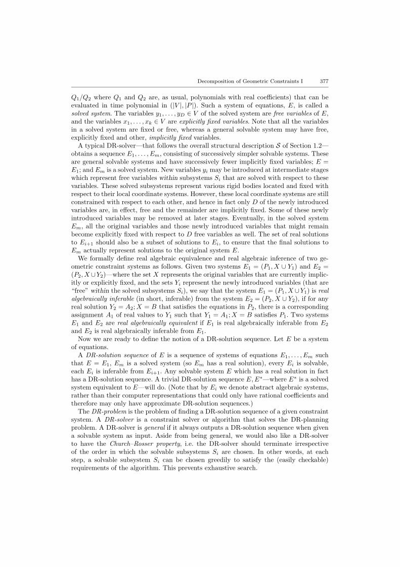
is being generated—i.e. the DR-solver exactly fits the structural description S given inthe previous section. Furthermore, we will define the DR-solver in the general context ofpolynomial equations that arise from the geometric constraints.
In Section 3 we will shift our attention to the DR-planning problem. The DR-plannergenerates a decomposition plan a priori, which then drives the direct algebraic/numericsolver—together, they form a DR-solver. The DR-planner, however, will be defined inthe context of constraint graphs that incorporate geometric degrees of freedom. TheDR-planner and its performance measures will be analogous to the italics terms definedhere.
In order to formally define DR-solvers and their performance measures, we need tospecify the model of real-algebraic computation used by the algebraic/numeric solver inFigure 3. However, the issue of the model or how real numbers are represented is en-tirely outside the focus of this manuscript for the following reason: our DR-solvers andperformance measures are robust in that they are conceptually independent of the alge-braic/numeric solver being used or how real numbers are represented. The definition ofDR-solvers and performance measures adapts straightforwardly to other natural modelsof computation. In other words, our conceptual definition of DR-solvers and performancemeasures are such that if DR-solver A performs better than DR-solver B with respect toone of our performance measures, then it continues to do so irrespective of the (natural)model of computation being used by the algebraic/numeric solver.
Further, as pointed out in an earlier note, this paper only emphasizes the boldfacecomponents of Figure 3, specifically the DR-planner, whose operation defined in Section 3will be seen to be purely combinatorial. In particular, no emphasis is placed on the non-boldface components, which includes the algebraic/numeric solver, and the model ofcomputation it uses.
Having noted the above, the model of computation we assume—for the the sake ofcompleteness and formality of definitions in this manuscript—is the Blum–Shub–Smalemodel of real algebraic computation (Blum et al., 1989). Briefly, in this model, real num-bers are assumed to be representable as such as entities, without any recourse to rationalapproximations and finite precision or interval arithmetic. Real arithmetic operationssuch as multiplication and addition and division can be performed in constant time, andfinding an unambiguous representation of each real zero of a univariate polynomial p canalso be achieved in time polynomial in the degree of p. Furthermore, these unambiguousrepresentations of real zeroes of univariate polynomials are treated as entities just likeany other real number, and can for instance, be used as coefficients of other polynomials.
A system of equations E is a pair (P,X) where P is a set of polynomial equationswith real coefficients, and X is a set of formal indeterminates. The union of two systemsE1 = (P1, X1) and E2 = (P2, X2) is the system (P1 ∪ P2, X1 ∪ X2). An intersectionE1 ∩ E2 is the system (P1 ∩ P2, X1 ∩X2).
Within the geometric context, a solved subsystem is a rigid or solvable system whereall the variables have already been “solved for”, i.e. they have typically been expressedexplicitly as polynomials of D free variables, where D represents the number of degrees offreedom of the rigid body (within its local coordinate system) in the prevailing geometry.In some cases, for example when the rigid body is a line in three dimensions, the numberof free variables, including redundant ones, may be greater than D.
Let E = (P, V ) with V = {y1, . . . , yD} ∪ X be such that every equation in P is oftype xj = Fj(y1, . . . , yD), for all xj ∈ X and Fj is a rational function (of the form
Decomposition of Geometric Constraints I 377
Q1/Q2 where Q1 and Q2 are, as usual, polynomials with real coefficients) that can beevaluated in time polynomial in (|V |, |P |). Such a system of equations, E, is called asolved system. The variables y1, . . . , yD ∈ V of the solved system are free variables of E,and the variables x1, . . . , xk ∈ V are explicitly fixed variables. Note that all the variablesin a solved system are fixed or free, whereas a general solvable system may have free,explicitly fixed and other, implicitly fixed variables.
A typical DR-solver—that follows the overall structural description S of Section 1.2—obtains a sequence E1, . . . , Em, consisting of successively simpler solvable systems. Theseare general solvable systems and have successively fewer implicitly fixed variables; E =E1; and Em is a solved system. New variables yi may be introduced at intermediate stageswhich represent free variables within subsystems Si that are solved with respect to thesevariables. These solved subsystems represent various rigid bodies located and fixed withrespect to their local coordinate systems. However, these local coordinate systems are stillconstrained with respect to each other, and hence in fact only D of the newly introducedvariables are, in effect, free and the remainder are implicitly fixed. Some of these newlyintroduced variables may be removed at later stages. Eventually, in the solved systemEm, all the original variables and those newly introduced variables that might remainbecome explicitly fixed with respect to D free variables as well. The set of real solutionsto Ei+1 should also be a subset of solutions to Ei, to ensure that the final solutions toEm actually represent solutions to the original system E.
We formally define real algebraic equivalence and real algebraic inference of two ge-ometric constraint systems as follows. Given two systems E1 = (P1, X ∪ Y1) and E2 =(P2, X ∪Y2)—where the set X represents the original variables that are currently implic-itly or explicitly fixed, and the sets Yi represent the newly introduced variables (that are“free” within the solved subsystems Si), we say that the system E1 = (P1, X ∪Y1) is realalgebraically inferable (in short, inferable) from the system E2 = (P2, X ∪ Y2), if for anyreal solution Y2 = A2;X = B that satisfies the equations in P2, there is a correspondingassignment A1 of real values to Y1 such that Y1 = A1;X = B satisfies P1. Two systemsE1 and E2 are real algebraically equivalent if E1 is real algebraically inferable from E2
and E2 is real algebraically inferable from E1.Now we are ready to define the notion of a DR-solution sequence. Let E be a system
of equations.A DR-solution sequence of E is a sequence of systems of equations E1, . . . , Em such
that E = E1, Em is a solved system (so Em has a real solution), every Ei is solvable,each Ei is inferable from Ei+1. Any solvable system E which has a real solution in facthas a DR-solution sequence. A trivial DR-solution sequence E,E∗—where E∗ is a solvedsystem equivalent to E—will do. (Note that by Ei we denote abstract algebraic systems,rather than their computer representations that could only have rational coefficients andtherefore may only have approximate DR-solution sequences.)
The DR-problem is the problem of finding a DR-solution sequence of a given constraintsystem. A DR-solver is a constraint solver or algorithm that solves the DR-planningproblem. A DR-solver is general if it always outputs a DR-solution sequence when givena solvable system as input. Aside from being general, we would also like a DR-solverto have the Church–Rosser property, i.e. the DR-solver should terminate irrespectiveof the order in which the solvable subsystems Si are chosen. In other words, at eachstep, a solvable subsystem Si can be chosen greedily to satisfy the (easily checkable)requirements of the algorithm. This prevents exhaustive search.

378 C. M. Hoffman et al.
Next, we formally define a set of performance measures for the DR-solution sequencesand DR-solvers. These performance measures are designed to capture the characteristicsC of constraint solvers given in Section 1.3, that are desirable for engineering designand assembly applications. (Note that many of these measures are Boolean, i.e. eithera certain desirable condition is met or not.) In particular, we would like a DR-solutionsequence Q = E1, . . . , Em of a solvable system E to have several properties. To describethese properties we formalize a simplifying map from each system Ei to its successorEi+1. In fact, for generality, we choose these maps Ti—called subsystem simplifiers—tomap the set of subsystems of Ei onto the set of subsystems of Ei+1.
First, in order to reflect the Church–Rosser property in (i), and points (iv) and (vi)of C, we would like these subsystem simplifiers Ti to be natural and well-behaved, i.e. toobey the following simple and non-restrictive rules.
(1) If A is a subsystem of B, then Ti(A) is a subsystem of Ti(B).(2) Ti(A) ∪ Ti(B) = Ti(A ∪B).(3) Ti(A) ∩ Ti(B) = Ti(A ∩B).
Second, in the description of the typical DR-solver S given in Section 1.2, each systemEi+1 in the DR-solution sequence is typically to be obtained from Ei by replacing asolvable subsystem Si in Ei (located during Step 1 of S), by a simpler subsystem (duringSteps 2 and 3). For a manipulable DR-solution sequence (again satisfying points (i), (iv),(v) and (vi) of C), we would like Ei+1 to look exactly like Ei outside of Si. This leads toanother set of properties desirable for the subsystem simplifiers Ti.
(4) Each Ei = Si∪Ri∪Ui, 1 ≤ i ≤ m, where Si is solvable, Ri is a maximal subsystemsuch that Si and Ri do not share any variables, Si, Ri, Ui do not share any equations,and all variables of Ui are either variables of Si or Ri. For any A ⊆ Ri, Ti(A) = A.
Thirdly, in order to address points (iv)–(vi), and (i) of C simultaneously, i.e. permittinggenerality of the subsystem Si that is replaced by a simpler system during the ith step,while at the same time making it convenient for the designer to geometrically followand manipulate the decomposition, we would like the subsystem simplifiers to satisfy thefollowing property.
(5) For each i, all the pre-images of Si, T−1j . . . T−1
i−1(Si), 1 ≤ j ≤ i−1, are algebraicallyinferable from Si, and furthermore, they are solvable or rigid subsystems for thegiven geometry (recall that the definition of “solvable” depends on the geometry).It follows from (2) and (3) above that the inverse T−1
i (A) =⋃B where the union
is taken over all B ⊆ Ei, such that Ti(B) ⊆ A.
The above property states that while the subsystem simplifiers enjoy a high degreeof generality and are completely free to map solvable subsystems into solvable systems,they should never map (convert) subsystems that are originally not solvable into one ofthe chosen, solvable systems Si, at any stage i. In other words, in the act of simplify-ing, the subsystem simplifiers should not create one of the solvable subsystems Si outof subsystems that were originally not solvable. A DR-solution sequence that satisfiesthe above properties is called valid. Thus a valid DR-solution sequence for a geometricconstraint system E is specified as a sequence of E1, . . . , Em such that E1 = E, Em is a

Decomposition of Geometric Constraints I 379
solved system, every Ei is solvable and inferable from Ei+1, every Ei = Si ∪ Ri ∪ Ui asdescribed above.
The motivation given for each of the properties above makes it clear that valid DR-solution sequences encompass highly general but geometrically meaningful solutions ofthe original constraint system E. Next we turn to point (ii) of C, i.e. optimality, whichalso competes with generality (point (i)). For optimality, we would like to minimize thesize of the largest solvable subsystem Si in the DR-solution sequence. Formally, the sizeof the DR-solution sequence Q is equal to max1≤i≤m |Si|, where the size |Si| is equalto the total number of its variables less the number of its explicitly fixed variables. Theoptimal DR-size of the algebraic system E is the minimum size of Q, where the minimumis taken over all possible DR-solution sequences Q of E. An optimal DR-solution sequenceQ of E is a solution sequence such that the size of Q is equal to the optimal DR-size ofE. The approximation factor of the DR-solution sequence Q of the system E is definedas the ratio of the optimal DR-size of E to the size of Q.
As a general rule for optimality, it is clear that the larger the choice for solvablesubsystems Si of Ei available at any stage i, the more likely that one can find a smallsolvable Si in Ei. In other words, we would like to make sure that the subsystem simplifierdoes not destroy solvability of too many subsystems starting from the original system E.Note that while the definition of DR-solution sequence makes sure that the entire systemEm is solvable if E1 is, it does not require the same for subsystems of Ei. (In fact, evenif all the Ei in a DR-solution sequence are algebraically equivalent, this would still notimply that solvability is preserved for the subsystems.) In addition, while the definitionof a DR-solution sequence ensures that Ei+1 has a real solution if Ei has one, it doesnot ensure the same for subsystems of Ei. The next two definitions capture propertiesof subsystem simplifiers that preserve subsystem solvability (resp. solutions) to varyingdegrees, thereby helping the optimality of the DR-solver, i.e. (ii) of C. The DR-solutionsequence Q = E1, . . . , Em is solvability preserving if and only if for all A ⊂ Ei, A issolvable (resp. has a real solution) and (A ∩ Si = ∅ or A ⊂ Si) ⇐⇒ Ti(A) is solvable(resp. has a real solution). A DR solution sequence Q = E1, . . . , Em is strictly solvabilitypreserving if and only if for all A ⊂ Ei, A is solvable (resp. has a real solution)⇐⇒ Ti(A)is solvable (resp. has a real solution). Requiring such a solvability preserving simplifierplaces a weak restriction on the class of valid DR-solution sequences, but on the otherhand, this restriction cannot eliminate all optimal DR-solution sequences. Furthermore,solvability preservation helps to ensure the Church–Rosser property in (i) of C.
Note. To be more precise, “solvability preservation” should be termed “solvability andsolution-existence preservation”, but we choose the shorter phrase.
In fact, for DR-solution sequences to be optimal, we would prefer that for all i ≥ 1,Si does not contain any strictly smaller subsystem, say B that is solvable, and has notbeen found (during Step 1 of the description S in Section 1.2) and simplified/replacedat an earlier stage j < i. The DR-solution sequence Q = E1, . . . , Em is complete if andonly if for every non-trivial solvable B ⊂ Si, B = Ti−1Ti−2 . . . Tj(Sj) for some j ≤ i− 1.While the completeness requirement restricts the class of valid DR-solution sequences,it only eliminates sequences that either have size greater than optimal or the same sizeas some optimal sequence that does simplify B. In addition to affecting optimality, i.e.(ii) of C, completeness also strongly reflects (ix): completeness prevents a DR-solver from

380 C. M. Hoffman et al.
overlooking an overconstrained subsystem inside a well-constrained subsystem, which isalso useful for constraint reconciliation (see Hoffmann and Joan-Arinyo, 1998).
So far, we have discussed performance measures that measure the desirability of DR-solution solution sequences. Next we formally define directly analogous performance mea-sures for DR-solvers which generate DR-solution sequences. A DR-solver A is said to bevalid, solvability preserving, strictly solvability preserving, complete if and only if for everyinput constraint system E, every DR-solution sequence produced by A is valid, solvabilitypreserving, strictly solvability preserving or complete, respectively.
Note. Purely as a tool to help analysis and exposition, often we assume that DR-solversfor producing DR-solution sequences are randomized or non-deterministic in a naturalway, i.e. those steps in the algorithm where arbitrary choices of equations or variablesare made (for example, to be the lowest numbered equation or variable) are now takento be randomized or non-deterministic choices.
The next definition formalizes performance measures related to characteristic (ii) ofC that differentiates randomized DR-solvers for which some random choice leads to anoptimal DR-solution sequence, from inferior DR-solvers where no choice would lead toan optimal DR-solution sequence. The worst-choice approximation factor of a DR-solverA on input system E is the minimum of the approximation factors of all DR-solutionsequences Q of E obtained by the algorithm A over all possible random choices. Thebest-choice approximation factor of the algorithm A on input E is the maximum of theapproximation factors of all the DR-solution sequences Q of E obtained by the algorithmA over all possible random choices.
3. Formal Definition of a DR-planner Using Constraint Graphs
The DR-solution sequence defined in the previous section embeds a DR-plan that isintertwined with the actual solution of the system. Therefore, a DR-solver that simplyoutputs a DR-solution sequence (even one that is strictly solvability preserving, complete,etc.), may not be modular as shown in Figure 3.
How does one construct a DR-solver that first generates a DR-plan before using it todrive the general algebraic/numeric solver? First note that repeatedly applying Steps 1and 3 of the DR-solver in the description S in Section 1.2 could potentially generate aDR-plan without actually solving any subsystem (and without applying Step 2), providedthat the following can be done:
(a) solvability of a subsystem Si of the system Ei in Step 1 can be determined generi-cally, without actually solving it; and
(b) a solvable subsystem Si can be replaced in Step 3 without actually solving Si—i.e.by a hypothetical solved subsystem—to give the new system Ei+1. For this we needa consistent and adequate abstraction of the systems Ei, and of their subsystems,as well as a way to abstract a hypothetical solved subsystem. In other words, weneed to adapt the subsystem simplifier maps described in the last section, so thatthe iteration can proceed with Step 1 again.
By thus modifying the description S of the DR-solver, we obtain a DR-planner whichcan be employed as a pre-processing step to output a DR-plan instead of a DR-solution

Decomposition of Geometric Constraints I 381
2
2
1
1 1
E
FD
2
Figure 4. A constraint graph.
sequence. This DR-plan can thereafter be used to direct a series of applications of Step 2,leading to a complete DR-solution sequence. This modularity helps, for example, towardsmanoeuverability by the designer (point (vi)), and towards compatibility of the DR-solverwith existing solvers (point (v)).
In order to formally define such a DR-plan, we follow a common practice and view theconstraint system as the constraint hypergraph: this abstraction permits us to build theDR-planner on the foundation of generalized degree of freedom analysis which is known towork well in estimating generic solvability of constraint systems without actually solvingthem. (This is explained more precisely after the formal graph-theoretic definitions are inplace.) Hence using constraint graphs facilitates both tasks (a) and (b) described above.
In other words a DR-planner that is based on a generalized degree of freedom analysisis robust in the following sense: changing the numerical values of constraints is notlikely to affect the DR-plan. Thus the motivation for using constraint graphs includesall of the desirable characteristics (iii) to (vi) of the set C in Section 1.3. In addition,geometry is more visibly displayed via constraint graphs than via equations, therebyhelping interaction with the designer.
Note. DR-plans and planners and their performance measures could also be defineddirectly in terms of the algebraic constraint systems, just as we defined DR-solvers.In this paper, however, due to the reasons mentioned above, we define DR-plans andplanners entirely within the context of constraint graphs and degree of freedom analysis.
3.1. constraint graphs and solvability
First we define the abstraction that converts a geometric constraint system into aweighted graph. Recall that a geometric constraint problem consists of a set of geometricobjects and a set of constraints between them.
A geometric constraint graph G = (V,E,w) corresponding to a geometric constraintproblem is a weighted graph with n vertices (representing geometric objects) V andm edges (representing constraints) E; w(v) is the weight of vertex v and w(e) is theweight of edge e, corresponding to the number of degrees of freedom available to anobject represented by v and the number of degrees of freedom removed by a constraintrepresented by e, respectively. For example, Figure 4 is a constraint graph of a constraintproblem shown in Figure 1. Note that the constraint graph could be a hypergraph, eachhyperedge involving any number of vertices.
Now we introduce definitions that will help us to relate the notion of solvability of thegeometric constraint system to the corresponding geometric constraint graph.

382 C. M. Hoffman et al.
A subgraph A ⊆ G that satisfies∑e∈A
w(e) +D ≥∑v∈A
w(v) (1)
is called dense, where D is a dimension-dependent constant, to be described below. Thefunction d(A) =
∑e∈A w(e)−
∑v∈A w(v) is called the density of a graph A.
The constant D is typically(d+1
2
)where d is the dimension. The constant D captures
the degrees of freedom associated with the cluster of geometric objects correspondingto the dense graph. In general, we use words “subgraph” and “cluster” interchangeably.For planar contexts and Euclidean geometry, we expect D = 3 and for spatial contextsD = 6, in general. If we expect the cluster to be fixed with respect to a global coordinatesystem, then D = 0.
A dense graph with density strictly greater than −D is called overconstrained. A graphthat is dense and all of whose subgraphs (including itself) have density at most −D iscalled well-constrained. A graph G is called well-overconstrained if it satisfies the follow-ing: G is dense, G has at least one overconstrained subgraph, and has the property thaton replacing all overconstrained subgraphs by well-constrained subgraphs, G remainsdense. A graph that is well-constrained or well-overconstrained is said to be solvable. Adense graph is minimal if it has no proper dense subgraph. Note that all minimal densesubgraphs are solvable, but the converse is not the case. A graph that is not solvableis said to be underconstrained. If a dense graph is not minimal, it could in fact be anunderconstrained graph: the density of the graph could be the result of embedding asubgraph of density greater than −D.
In order to understand how solvable constraint graphs relate to solvable constraint sys-tems it is important to remember that a geometric constraint problem has two aspects—combinatorial and geometric. The geometric aspect deals with actual parameters of thegeometric constraint problem, while the combinatorial aspect deals with only the abstrac-tions of objects and constraints. Unfortunately, at the moment it is not known how tocompletely separate the two aspects, except for some special cases. In this paper we willlimit ourselves to the geometric constraint problems where generally there is a correspon-dence between solvable constraint systems and solvable constraint graphs. In order to dothat, we need to introduce and formalize the notion of generic solvability of constraintsystems. Informally, a constraint system is generically (un)solvable if it is (un)solvable formost choices of coefficients of the system. More formally we use the notion of genericityof e.g. Cox et al. (1998). A property is said to hold generically for polynomials f1, . . . , fnif there is a non-zero polynomial P in the coefficients of the fi such that this propertyholds for all f1, . . . , fn for which P does not vanish.
Thus the constraint system E is generically (un)solvable if there is a non-zero poly-nomial P in the parameters of the constraint system—such that E is (un)solvable whenP does not vanish. Consider for example Figure 5. Here the objects are six points in 2Dand the constraints are eight distances between them. This system is unsolvable since theedge BC can be continuously displaced, unless the length of AD (induced by the lengthsof AE,DE,DF,AF and EF ) is equal to |AB| + |BC| + |CD|. Since we can create anappropriate non-zero polynomial P (AB,BC, . . . , EF ), such that P () = 0 if and only if|AD| = |AB|+ |BC|+ |CD|, this system is generically unsolvable.
While a generically solvable system always gives a solvable constraint graph, the con-verse is not always the case. In fact, there are solvable, even minimal dense graphs whosecorresponding systems are not generically solvable, and are in fact generically not solv-

Decomposition of Geometric Constraints I 383
BC
D
E
F
A
Figure 5. Generically unsolvable system.
A
B
CD
E
F
G
H 3
3
3
3
3
3
3
3
Figure 6. Generically unsolvable system that has a solvable constraint graph.
able (note that the position of the “not” changes the meaning, the latter being strongerthan the former). Consider for example Figure 6. The constraint system is shown on theleft, it consists of eight points in 3D and 18 distances between them. The correspondingconstraint graph is shown on the right, the weight of all the edges is 1, the weight of thevertices is 3, the geometry-dependent constant D = 6. Note that this system is gener-ically unsolvable since rigid bodies ABCDE and AFGHE can rotate about the axispassing through AE. This example can also be transformed into a constraint problem in2D, where the objects are circles and the constraints are angles of intersections (Saliolaand Whiteley, 1999).
Another example is the graph K7,6 that in four dimensions represents distances be-tween pairs of points. The constraint graph is minimal dense but it does not represent agenerically solvable system.
It should be noted that in two dimensions, according to Laman’s (1970) theorem,if all geometric objects are points and all constraints are distance constraints betweenthese points, then any minimal dense subgraph represents a generically solvable system.In addition, there exists a purely combinatorial characterization of solvable systems inone dimension based on connectivity of the constraint graphs. However, as examplesabove indicate, the generalization of Laman’s theorem fails in higher dimensions even forthe case of points and distances.
There is a matroid-based approach to verifying whether solvability of the constraintgraph implies solvability of the constraint system. It begins by checking whether a sub-

384 C. M. Hoffman et al.
modular function f(E) = 2|V |−3, defined on sets of edges of the constraint graph, createsa matroid (Whiteley, 1992, 1997), i.e. checking whether the created function is positiveon single edges. Thereafter this approach checks whether the corresponding geometricstructure is generically rigid. Some matroid-based approaches to determining generic solv-ability are fast in practice, for example those to be discussed later in Section 4.2 under“Generalized Maximum Matching”. However, so far no match has been established (forall cases) between the created matroid and generic rigidity of the particular geometricproblem.
There are several attempts at characterization of generic solvability in dimension threeand higher for the case of points and distances (Graver et al., 1993; Tay, 1999). One suchcharacterization, the so-called Henneberg construction, checks whether a given constraintgraph can be constructed from the initial basic graph by applying a sequence of standardreplacements. A characterization due to Dress checks whether the constraint graph sat-isfies a certain inclusion–exclusion type rule. A characterization due to Crapo examineswhether the constraint graph can be decomposed into a union of certain edge-disjointtrees. All of these characterizations though interesting and useful, are so far unprovenconjectures.
Note. Due to the above discussion, we restrict ourselves to the class of constraint sys-tems where solvability of the constraint graph in fact implies the generic solvability ofthe constraint system. (As pointed out earlier, the converse is always true, with no as-sumptions on the constraint system.)
As was indicated above, this class is far from empty, it contains all constraint problemsinvolving points and distances in 2D, problems resulting from Cauchy triangulations ofthe polyhedra in 3D as well as body-and-hinge structures in 3D. Moreover, it shouldbe emphasized that while existing applications stop at finding subgraphs representingsolvable constraint systems, we are interested in the entire problem of decompositionand recombination, optimizing the size of the largest subsystem to be solved, i.e. we areinterested in finding an optimal DR-plan. In addition, note that for the class of generi-cally solvable constraint systems and corresponding graphs, the DR-planning problem isalready, in general, difficult (see a later note about NP-hardness, after the definition ofthe optimal DR-plan).
3.2. formal definition of DR-plans using constraint graphs
Informally, stated in terms of constraint graphs, the DR-planning problem involvesfinding a sequence of graphs Gi—a DR-plan—such that the original constraint graphG = G1 and every Gi contains a minimal solvable subgraph Si, which is simplified orabstracted into a simpler subgraph Ti(Si) and substituted into Gi to give an overallsimpler graph Gi+1 = Ti(Gi). (While Ti(Si) should be simpler than Si, it should also besomehow equivalent to Si, for example by having the same density value.) If the originalgraph G1 is well-constrained, then the process terminates when Gm = Sm. (If not, theprocess terminates with the decomposition of Gm into a maximal set of minimal solvablesubgraphs.)
Consider for example Figure 7 which shows one simplification step. On the left is theconstraint graph G1, the weight of all vertices is 2, the weight of all edges is 1, thegeometry-dependent constant D = 3. Then S1 = {A,B,C} is a solvable subgraph. On

Decomposition of Geometric Constraints I 385
S1
A
B
C
G
H
ID E
F
V
I
H
ED
F
G
Figure 7. Original geometric constraint graph G1 and simplified graph G2.
the right is the simplified graph T1(G1) = G2, after subgraph S1 is replaced by a vertex{V } = T1(S1). Since the density of the subgraph S1 is −3, the weight of the vertex {V }could be set to 3.
A sequence of simplification steps is shown in Figure 8. The top part depicts a ge-ometric constraint graph G, where the weight of each edge is 1, the weight of eachvertex is 2, and the dimension-dependent constant D is equal to 3 (this correspondsto points and distances in 2D). One of the plans for decomposing and recombiningG (and the geometric constraint system that G represents) into small solvable sub-graphs (representing solvable subsystems), is to decompose G into dense subgraphsS1 = {A,B,C}, S2 = {D,E, F}, S3 = {G,H, I}, S5 = {J,K,L}, S6 = {M,N,O}; repre-sent their solutions appropriately in a simplified graph so that they can be recombined,one possibility is to represent them as vertices P,Q,R, S, T of weight 3 each; recursivelydecompose the simplified graph into S4 = {P,Q,R}, S7 = {S, T}; represent and recom-bine their solutions as vertices U,W of weight 3; and so on until the entire graph isrepresented and recombined as a single vertex.
A corresponding DR-plan is shown at the bottom part of Figure 8. Note that therecould be more than one DR-plan for a given constraint graph. For example, anotherpossible DR-plan for a constraint graph described above is shown in Figure 9.
An optimal DR-plan will minimize the size of the largest solvable subgraph Si foundduring the process. That is, it will minimize the maximum fan-in of the vertices in theDR-tree shown in Figures 8 and 9, where by fan-in of a vertex we mean the numberof immediate descendants of the vertex. With this description, it should be clear thatDR-plans obtained using the weighted, constraint graph model are generically robustwith respect to the changes made to the geometric constraints; as long as the number ofdegrees of freedom attached to the objects and destroyed by the constraints remains thesame, the same DR-plan will work for the changed constraint system as well. Thus, suchDR-plans satisfy the initial robustness requirements of characteristic (viii) of the set Cdescribed in Section 1.3.
Next we formally define a DR-plan for constraint graphs, and the various performancemeasures that capture desirable properties of DR-plans and DR-planners. The develop-ment is parallel to that in Section 2, where a DR-solution sequence and various perfor-

386 C. M. Hoffman et al.
S4
S2
S1
S3 S5S6
S
S
S S S S
S
S12 3
4
8
7
5 6
7S
S 8
B
A C
D E
F
G
H
I
J
K
L M
N
O
A B C D E F G H I J K L M N O
Figure 8. Geometric constraint graph and a DR-plan.
mance measures for these sequences and for DR-solvers were motivated and defined interms of polynomial systems.
Note. Due to the strong analogy of DR-planners to DR-solvers defined in the previoussection, the discussion here is more terse. The following are useful generic correspondencesto keep in mind after reading the note at the end of Section 3.1, and the paragraphspreceding it:
Solvable subgraphs solvable subsystems;DR-plans DR-solution sequences;DR-planner DR-solver;subgraph simplifier subsystem simplifier.
Let G be a solvable constraint graph. A DR-plan Q for G is a sequence Q of graphsG1, . . . , Gm such that G1 = G, Gm is a minimal solvable graph, and every Gi is solvable.An algorithm is a general DR-planner if it outputs a DR-plan when given a solvableconstraint graph as input.
The union (resp. intersection) of two subgraphs A and B is the graph induced by the

Decomposition of Geometric Constraints I 387
S2
S1
S3 S5
S4
S
S
S
SS S S S
8
6
7
5
4
12
3
S6
S7
S8
A B C D E F G H I J K L M N O
B
A C
D E
F
G
H
I
J
K
L M
N
O
Figure 9. Another possible DR-plan.
union (resp. intersection) of sets of vertices of A and B. All subgraphs are understood tobe vertex induced.
The mapping from the graph Gi to Gi+1 is called a subgraph simplifier and is denotedby Ti. This mapping should have the following properties.
(1) If A is a subgraph of B, then Ti(A) is a subgraph of Ti(B).(2) Ti(A) ∪ Ti(B) is the same as the graph Ti(A ∪B).(3) Ti(A) ∩ Ti(B) is the same as Ti(A ∩B).
As in the case of DR-solution sequences, assume that every constraint graph Gi in theDR-plan can be written as Si ∪ Ri ∪ Ui, where Si is minimal solvable, Ri is a maximalsubgraph such that Si and Ri do not have common vertices, Si, Ri, Ui do not havecommon edges and all vertices of Ui are either vertices of Si or vertices of Ri. Analogousto properties (4) and (5) of the subsystem simplifier in the previous section, we wouldlike the subgraph simplifier to have the following additional properties.
(4) For every A ⊆ Ri, Ti(A) = A.(5) All the pre-images of Si, i.e. T−1
j T−1j+1 . . . T
−1i−1(Si) for all 1 ≤ j < i−1, are solvable.

388 C. M. Hoffman et al.
A DR-plan that satisfies the above rules is called valid. The size of the DR-plan Q of Gis the maximum of the sizes of Si. The size of an arbitrary subgraph A ⊆ Gi is computedas follows.
Size(A) = 0For 1 ≤ j ≤ i− 1
B = Ti−1Ti−2 . . . Tj(Sj)If A ∩B 6= 0
then Size(A) = Size(A) +D,A = A \Bend if
end forSize(A) = Size(A) +
∑v∈A w(v)
In other words, the image of any of the Sj contributes D to the size of A, where Dis a geometry-dependent constant, and the vertices of A that are not in any such im-age contribute their original weight. The optimal size of the constraint graph G is theminimum size of Q, where the minimum is taken over all possible DR-plans of G. Anoptimal DR-plan of G is the DR-plan that has size equal to the optimal size of G. Theapproximation factor of DR-plan Q of the graph G is defined as the ratio of the optimalsize of G to the size of Q.
Note. The problem of finding the optimal DR-plan for a constraint graph with un-bounded vertex weights is NP-hard. This follows from a result in the authors’ paper(Hoffmann et al., 1997) showing that the problem of finding a minimum dense subgraphis NP-hard, by reducing this problem to the CLIQUE. The CLIQUE problem is ex-tremely hard to approximate (Hastad, 1996), i.e. finding a clique of size within a n1−ε
factor of the size of the maximum clique cannot be achieved in time polynomial in n,for any constant ε (unless P = NP). However our reduction of CLIQUE to the optimalDR-planning problem is not a so-called gap-preserving reduction (or L-reduction); thushow well this problem could be approximated is still an open question.
The definition of solvability preservation is largely analogous to the case of DR-solvers,but is additionally motivated by the following. In the case of DR-solvers, one conditionon a solvability preserving simplifier is that it preserves the existence of real solutions forcertain subsystems. Here, in the case of DR-plans, a natural choice is to correspondinglyrequire that the simplifier does not map well-constrained subgraphs or overconstrainedsubgraphs to underconstrained and vice versa. The DR-plan Q of G is solvability pre-serving if and only if for all A ⊂ Gi, A is solvable and (A ∩ Si = ∅ or A ⊂ Si) ⇐⇒Ti(A) is solvable. The DR-plan Q of G is strictly solvability preserving if and only if forall A ⊂ Gi, A is solvable ⇔ Ti(A) is solvable. The DR-plan Q of G is complete if andonly if for all non-trivial solvable B ⊂ Si, B = Ti−1Ti−2 . . . Tj(Sj) for some j ≤ i− 1.
Next, we formally define DR-planners and their performance measures. An algorithmis said to be a DR-planner if it outputs a DR-plan when given a solvable constraintgraph as input. As before, we consider DR-planners to be randomized algorithms. Arandomized DR-planner A is said to be valid, solvability preserving, strictly solvabilitypreserving, complete if and only if for every G every DR-plan produced by A is valid,solvability preserving, strictly solvability preserving or complete, accordingly. The worst-choice approximation factor of a DR-planner A on input graph G is the minimum of

Decomposition of Geometric Constraints I 389
the approximation factors of all DR-plans Q of G obtained by the DR-planner A overall possible random choices. The best-choice approximation factor of the algorithm A oninput graph G is the maximum of the approximation factors of all the DR-plans Q of Gobtained by the DR-planner A over all possible random choices.
In addition to the above performance measures, we define three others that reflect theChurch–Rosser property, the ability to deal with underconstrained subsystems, as wellas the ability to incorporate an input, design decomposition provided by the designer.
A DR-planner is said to have the Church–Rosser property, if the DR-planner terminateswith a DR-plan irrespective of the order in which the dense subgraphs Si are chosen.
A DR-planner A adapts to underconstrained constraint graphs G if every (partial)DR-plan produced by A terminates with a set of solvable subgraphs Qi such that eachsolvable subgraph Qi has no supergraph that is solvable, and moreover, no subgraph ofG that is disjoint from all of the Qi’s is solvable.
A conceptual design decomposition P is a set of solvable subgraphs Pi, which are par-tially ordered with respect to the subgraph relation. A DR-planner A is said to incorpo-rate a design decomposition P , if for every DR-plan Q produced by A, the correspondingsequence of solvable subgraphs Si embeds a topological ordering of P as a subsequence—recall that a topological ordering is one that is consistent with the natural partial ordergiven by the subgraph relation on P .
When a DR-plan incorporates a design decomposition P , the level of a cluster Pi inthe partial ordering of P can now be viewed as a priority rating which specifies whichcomponent of the design decomposition has most influence over a given geometric object.In other words, a given geometric object K is first fixed/manipulated with respect to thelocal coordinate system of the lowest level cluster Pi ∈ P containing K. Thereafter, theentire cluster Pi can be treated as a unit and can be independently fixed/manipulatedin the local coordinate system of the next level cluster Pj containing (the simplificationof) Pi, etc.
Finally, we summarize how the above formal performance measures capture the infor-mally described characteristics in the set C given in Section 1.3. The property of being ageneral DR-planner refers to whether the method successfully terminates with a DR-planin the general case, and reflects characteristic (i); since we use constraint graphs whichyield robust DR-plans that can be obtained efficiently, the property of being a generalDR-planner also reflects (iii) and (viii); dealing with underconstrained graphs also re-flects (i); incorporating input, design decompositions reflects (v); validity influences theChurch–Rosser property and reflects (i) as well as (iv), (v), (vi); solvability preservation,strict solvability preservation influences the Church–Rosser property and reflects (i), (ii),(iv), (v); completeness is based on criteria (ii) and (ix); worst- and best-choice approxi-mation factors are based on (ii) and complexity directly reflects (iii).
4. Performance Analysis of Prior DR-planners
We concentrate on two primary types of prior algorithms for constructing DR-plansusing constraint graphs and geometric degrees of freedom.
Note. Due to reasons discussed in Section 3, we leave out those graph rigidity-basedmethods for distance constraints in dimensions three or greater such as Tay and Whiteley(1985) and Hendrickson (1992) as well as methods such as Crippen and Havel (1988),Havel (1991) and Hsu (1996) since they are non-deterministic or rely on symbolic compu-

390 C. M. Hoffman et al.
tation, or they are randomized or generally exponential and based on exhaustive search.Graph rigidity- and matroid-based methods for more specific constraint graphs are dis-cussed in Section 4.2 under the so-called maximum matching-based algorithms. Also,for reasons discussed in the Introduction, we leave out methods based on decomposingsparse polynomial systems.
The first type of algorithm, which we call SR for constraint shape recognition (e.g.Owen, 1991, 1996; Hoffmann and Vermeer, 1994, 1995; Bouma et al., 1995; Fudos andHoffmann, 1996b, 1997), concentrates on recognizing specific solvable subgraphs of knownshape, most commonly, patterns such as triangles. The second type, which we call MM forgeneralized maximum matching (e.g. Kramer, 1992; Ait-Aoudia et al., 1993; Pabon, 1993;Latham and Middleditch, 1996), is based on first isolating certain solvable subgraphs bytransforming the constraint graph into a bipartite graph and finding a maximum general-ized matching, followed by a connectivity analysis to obtain the DR-plan. In this section,we give a formal performance analysis of SR- and MM-based algorithms—choosing a rep-resentative algorithm (typically the best performer) in each class—using the performancemeasures defined in the previous section.
Informally, one major drawback of the SR and MM algorithms is their inability toperform a generalized degree of freedom analysis. For example, SR would require aninfinite repertoire of patterns. In the case of spatial constraints, some elementary patternshave been identified (Hoffmann and Vermeer, 1994, 1995). In the case of extending thescope of planar constraint solvers, adding free-form curves or conic sections requiresadditional patterns as well (Hoffmann and Peters, 1995; Fudos and Hoffmann, 1996a).Similarly, a decomposition of underconstrained constraint graphs into well-constrainedcomponents is possible for SR algorithms but only subject to the pattern limitations. Inmany cases, MM algorithms will output DR-plans with larger, non-minimal subgraphsSi that may contain smaller solvable subgraphs. This affects the approximation factorsadversely.
This inability to find general minimal dense subgraphs also affects their ability todeal with overconstrained subgraphs that arise in assemblies, which is in turn needed toperform constraint reconciliation (Hoffmann and Joan-Arinyo, 1998).
4.1. constraint shape recognition (SR)
Consider the algorithm of Fudos and Hoffmann (1996b, 1997) which relies on thefollowing strong assumption (SR1): all geometric objects in two dimensions have 2 degreesof freedom and all constraints between them are binary and destroy exactly 1 degree offreedom. Thus, in the corresponding constraint graph, the weight of all the edges is 1 andof all the vertices is 2. Because of this assumption, the SR algorithm ignores the degreesof freedom and relies only on the topology of the constraint graph.
description of the algorithm
We give a terse description of the algorithm—the reader is referred to Fudos andHoffmann (1996b, 1997) for details. Our description is meant only to put the algorithminto an appropriate DR-planner framework that is suited for the performance analysis.
The algorithm consists of two phases. During Phase One, SR uses the bottom-upiterative technique of Itai and Rodeh (1978): in the current graph Gi (where G1 = G),

Decomposition of Geometric Constraints I 391
specific solvable graphs (clusters) are found that can be represented as a union of threepreviously found clusters that pairwise share a common vertex. Such configurations ofthree clusters are called triangles. The vertices of Gi represent clusters and edges of Girepresent constraints between clusters (initially due to SR1, every vertex and every edgeof G is a cluster). More specifically, once a triangle formed by three clusters has beenfound, the three vertices in Gi corresponding to these three clusters are simplified intoone new vertex in the simplified graph Gi+1. The edges of Gi+1 are induced by the edgesof the three old vertices. This is repeated for k steps until there are no more trianglesleft. If there is only one cluster left in Gk, then the algorithm terminates. Otherwise Gkserves as an input to Phase Two of the algorithm.
Before we describe Phase Two, we note that a so-called cluster graph Ci correspondingto Gi is used as an auxiliary structure for the purpose of finding triangles. Hence thepartial DR-plan produced during Phase One of the algorithm is of the form: (G1, C1), . . . ,(Gk, Ck). The vertices of the cluster graph Ci correspond to
• vertices of the original graph G1;• cluster vertices in the graph Gi; and• edges in G1 which have not been included into one of the cluster vertices in the
graphs Gi−1, . . . , G1.
In particular, the first cluster graph C1 contains one vertex for every vertex and everyedge of G1. The edges of the cluster graph Ci connect the vertices of Gi that representclusters to the original vertices from G1 that are contained in these clusters. Due to thestructure of cluster graphs, triangles in Gi are found by looking for specific 6-cycles inthe corresponding cluster graph Ci. These 6-cycles consist of three cluster vertices andthree original vertices. The new cluster graph Ci+1 is constructed from Ci by adding anew vertex ci representing the newly found cluster Si, and connecting it by edges to theoriginal vertices from G1 that are in the cluster Si. We also remove the three old clustervertices in Ci which together formed the new cluster Si. We note that this is the only wayin which cluster vertices are removed from cluster graphs. In particular, situations mayarise where two clusters (that share a single vertex) are represented by the same vertexin the graph Gi, but they are represented by distinct vertices in the cluster graph Ci.
During Phase Two, SR constructs the remainder of the DR-plan (Gk, Ck), . . . ,(Gm, Cm). First SR uses a global top–down technique of Hopcroft and Tarjan (1973)to divide Gk into a collection of triconnected subgraphs. These subgraphs are foundby recursively splitting the original graph using separators of size at most 2. Thus thetriconnected components can be viewed as the leaves of a binary tree T each of whoseinternal nodes corresponds to a vertex separator of size at most 2.
For every triconnected subgraph S in Gk, a new cluster vertex is created in the clustergraph Ck: similar to Phase One, this vertex replaces all vertices that represent existingclusters contained in S.
The next pair (Gk+1, Ck+1) in the DR-plan is found as in Phase One by finding a tri-angle in Gk, or effectively locating a 6-cycle in Ck. However, triangles in Gk have alreadybeen located in the course of constructing the tree T—these triangles were originally splitby the vertex separators at the internal vertices. Thus, if the original constraint graphG is solvable, the remainder of the DR-plan (Gk+1, Ck+1), . . . , (Gm, Cm) is formed byrepeated simplifications along a bottom up traversal of the tree T .
If the original graph was underconstrained, then it is still possible to construct a

392 C. M. Hoffman et al.
51
51
GG
CCM
O
F
G
D
LN
OM
FO
DG
PAD A
DDG
AE
FO
OM
G
F
O
A B C
D E F
G H
I J
K
L M
N O ON
ML
K
JI
HG
P
Figure 10. The original graph G = G1, the cluster graph C1 and the simplified graphs G5, C5.
DR-plan of its maximal well-constrained subgraphs, by introducing additional constraintsand making the original graph solvable. That is, in order to complete the bottom uptraversal of the tree T in Phase Two, additional constraints need to be introduced, tomake the whole graph solvable. For details, see Fudos and Hoffmann (1996b, 1997).
example
Consider Figure 10. During Phase One, the triangles ADE,ABE,BCE and CEF willbe discovered and simplified as P . During Phase Two, the remainder of the graph willbe divided into triconnected subgraphs P, PGKILN and OKHMJP , then PGKILNand OKHMJP are simplified and finally the union of P, PGKILN and OKHMJP issimplified.
defining the simplifier map
The same simplifier is used throughout Phase One and Two: replace a subgraph Siconsisting of a triangle of clusters in Gi (or triconnected subgraphs during Phase Two)by one vertex in Gi+1 representing this triangle. The subgraph Si is found as a 6-cycle inthe cluster graph Ci. The cluster graph Ci+1 is constructed as described in Phase One.
More formally, recalling the definitions in Section 3: let G be a constraint graph; thefirst graph G1 in the DR-plan is the original graph G. Let Gi = (V,E) be the currentgraph and let Si be a cluster found. Let A ⊆ Gi, A = (VA, EA). Then the image of Aunder the subgraph simplifier Ti is Ti(A) = A, if the intersection of A and Si is empty;otherwise Ti(A) = (VTi(A), ETi(A)) where VTi(A) is the set of all vertices of A that are

Decomposition of Geometric Constraints I 393
T1T
3C C2
FE
FC
CE
CB
2C
C
B
E
D
A
D
A
AB
EB
DE
AD
AE C1 A
D
E
B
C
EB
AB
CB
CE
G2G1
G3
C1
C
2
E
B
J
ON
K
ML
I
HG
FED
CBA B C
F
G
I J
K
L
O
C
F
G H
I J
K
L
O
1C
M
N
H
2C
M
N
Figure 11. Action of the simplifier on Gi and Ci during Phase One.
not vertices of Si plus a vertex ci that replaces the cluster Si. The set of edges ETi(A) isa set of all edges of A that are not edges of Si; the edges of EA that have exactly oneendpoint in Si will have this endpoint replaced by the vertex ci; and the edges of A thathave both endpoints in Si are removed.
Since the cluster Si in Gi is located by finding a 6-cycle in Ci, we need to describe howCi+1 is constructed from Ci, i.e. the effect that Ti has on Ci (formally, Ti is a map from(Gi, Ci) to (Gi+1, Ci+1)). To obtain Ci+1, we start with Ci and first add a new vertex cirepresenting the cluster Si, which is connected by edges to all the original vertices thatit contains. Finally, vertices in Ci—that represent clusters entirely contained in Si—areremoved, and edges adjacent to these vertices are also removed.
Figures 11 and 12 illustrate the action of the subgraph simplifier Ti on both Gi and Ci.
a further concession for SR
Observe that the SR algorithm is not a general DR-planner when input geometricconstraint graphs do not comply with assumption SR1. For example, for the graph shownin Figure 13, during Phase One, SR would not find any triangles and during Phase Two,it would conclude that the graph is underconstrained, even though the graph is well-constrained.
SR implementations may remedy some cases similar to this one. For instance, weight2 edges to weight 2 vertices often arise from incidence constraints between geometricelements of the same type (two coincident points or two coincident lines), and such casesare easily accounted for by working with equivalence classes of such vertices. Moreover,most planners will evaluate the density of a graph before announcing under- or over-constrained situations. Thus, an implementation of the SR algorithms of Fudos andHoffmann (1996b, 1997) may or may not construct a DR-plan for the graph of Figure 13

394 C. M. Hoffman et al.
C8
G
G
5T6T7T8T
5
7C6C
9
F
K
D
R
Q
PP
IL
LN
G
K
L
N
AJ
O
F
K
L
D
A
DG
DI
DN
IK
OF
I
D P
Q
KH
KO
KJ
JF
G
I
P
ON
K
J
H
ML
Figure 12. Action of the simplifier during Phase Two.
32
2
2
2
2
2
1
12
22
21
1
Figure 13. This solvable graph would not be recognized as solvable by SR.
depending on the original problem statement. It is clear that such heuristics enlarge theclass of solvable graphs, but fall short of decomposing all solvable constraint graphs.
However, even when input graphs do comply with SR1, and SR checks the overalldensity of a graph, SR could still mistake a graph that is not solvable for solvable.Figure 14 shows an example which the SR algorithm may process incorrectly: since thegraph contains no solvable triangles, SR proceeds immediately to Phase Two. DuringPhase Two, the triconnectivity of the entire graph could be erroneously construed to meanthat the graph is solvable. In fact, the graph does have density −3, which superficiallyseems to support such a conclusion. However, the graph is certainly not well-constrained:the eight vertices on the right form a subgraph of density −2; that is, an overconstrainedsubgraph. Moreover, if this overconstrained subgraph is replaced a subgraph of density−3, the resulting graph has density −4 revealing that it is not well-overconstrained either,and therefore not solvable.
Figure 14 demonstrates that the density calculation heuristics is insufficient to deter-mine the existence of minimal dense subgraphs of triconnected constraint graphs. Whatis needed is a general algorithm for finding minimal dense subgraphs.In order to give a performance analysis of the SR algorithm for those classes of constraintgraphs where it does produce a satisfactory DR-plan, we make a strong concession (SR2)

Decomposition of Geometric Constraints I 395
Figure 14. Weight of all vertices is 2, weight of all edges is 1.
that: only “triangular” structures are “acceptable” for the remainder of this section.That is, we modify the definitions of validity, solvability preserving, strictly solvabilitypreserving and completeness by replacing the words “solvable subgraph” by the followingrecursive definition: “either a subgraph that can be simplified into a single vertex bya sequence of consecutive simplifications of triangles of solvable subgraphs (using thesimplifier described in Section 4.1), or a vertex, edge or triconnected subgraph”.
performance analysis
In this section, we analyze the SR algorithm with respect to the various performancemeasures defined in Section 3.
Claim 4.1. Under the concession SR2, the SR algorithm is valid.
Proof. We will show that every pre-image—of the “solvable” cluster Si found at theith iteration of the SR algorithm—is also “solvable”, using the stricter SR2 definitionof “solvable”. It can be easily checked that the other requirements necessary for validityfrom Section 3 also clearly hold.
Let Si be a cluster that has been found in Gi by the SR algorithm (by locating a6-cycle in Ci). Then from the description of the algorithm, and by assertion SR2, thereis a sequence of simplifications, say Ti+1, . . . , Tm whose composition maps Si to a singlevertex. For every pre-image A ⊆ Gj A = T−1
j . . . T−1i−1(Si), for j ≤ i− 1, the composition
Tm ◦ · · · ◦ Ti ◦ Ti−1 ◦ · · · ◦ Tj will map A to a single vertex, hence A is “solvable”. 2
Claim 4.2. The SR algorithm is strictly solvability preserving under the concession SR2,and therefore is solvability preserving as well.
Proof. Let A be a “solvable” subgraph, i.e. there is a sequence of simplificationsA1, . . . , Am such that A = A1 and Am consists of only one vertex. If the intersectionof A and the currently found cluster Si is empty, then Ti(A) = A and it remains “solv-able”. If this intersection is not empty, then a subgraph B = A ∩ Si is simplified into anew cluster vertex ci = Ti(Si). We need to show that in this case Ti(A) remains “solv-able” as well. Suppose that some subgraph of B is a vertex of a 6-cycle in one of thecluster graphs formed during the simplification A1, . . . , Am. Then clearly the new clustervertex ci could perform the same function: i.e. it could also be a vertex in that 6-cycleof one of the cluster graphs formed during the simplification A1, . . . , Am. In addition, ifA was triconnected, then so is Ti(A). This proves that there is a sequence (essentially a
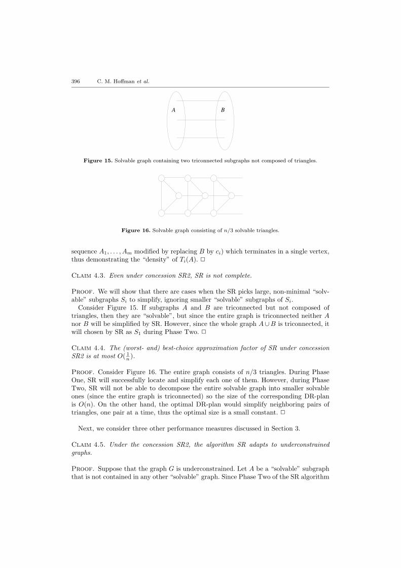
396 C. M. Hoffman et al.
A B
Figure 15. Solvable graph containing two triconnected subgraphs not composed of triangles.
Figure 16. Solvable graph consisting of n/3 solvable triangles.
sequence A1, . . . , Am modified by replacing B by ci) which terminates in a single vertex,thus demonstrating the “density” of Ti(A). 2
Claim 4.3. Even under concession SR2, SR is not complete.
Proof. We will show that there are cases when the SR picks large, non-minimal “solv-able” subgraphs Si to simplify, ignoring smaller “solvable” subgraphs of Si.
Consider Figure 15. If subgraphs A and B are triconnected but not composed oftriangles, then they are “solvable”, but since the entire graph is triconnected neither Anor B will be simplified by SR. However, since the whole graph A∪B is triconnected, itwill chosen by SR as S1 during Phase Two. 2
Claim 4.4. The (worst- and) best-choice approximation factor of SR under concessionSR2 is at most O( 1
n ).
Proof. Consider Figure 16. The entire graph consists of n/3 triangles. During PhaseOne, SR will successfully locate and simplify each one of them. However, during PhaseTwo, SR will not be able to decompose the entire solvable graph into smaller solvableones (since the entire graph is triconnected) so the size of the corresponding DR-planis O(n). On the other hand, the optimal DR-plan would simplify neighboring pairs oftriangles, one pair at a time, thus the optimal size is a small constant. 2
Next, we consider three other performance measures discussed in Section 3.
Claim 4.5. Under the concession SR2, the algorithm SR adapts to underconstrainedgraphs.
Proof. Suppose that the graph G is underconstrained. Let A be a “solvable” subgraphthat is not contained in any other “solvable” graph. Since Phase Two of the SR algorithm

Decomposition of Geometric Constraints I 397
is top–down, either SR will find A and simplify it as one of the Si’s, or A ∩ Si 6= ∅ forone of the Si. In either case, SR adapts to G. 2
Observation 4.6. Under the concession SR2, the SR algorithm has the Church–Rosserproperty, since the new graph Gi+1 remains “solvable” if Gi is “solvable”, regardless ofthe choice of the “solvable” Si that is simplified at the ith stage.
Claim 4.7. Under the concession SR2, the SR algorithm can incorporate design decom-positions P if and only if P fulfills the following requirement: any pair of “solvable”subgraphs Pk and Pt in P satisfy Pk ⊆ Pt or Pt ⊆ Pk or Pk ∩ Pt contains no edges.
Proof. For the “if” part we consider the most natural modification of the original SRalgorithm, and find a topological ordering O of the given design decomposition P—which is a set of “solvable” subgraphs of the input graph G, partially ordered under thesubgraph relation—such that O is embedded as a subplan of the final DR-plan generatedby this modified SR algorithm; i.e. O forms a subsequence of the sequence of “solvable”subgraphs Si, whose (sequential) simplification gives the DR-plan.
We take any topological ordering O of the given design decomposition P and createa DR-plan for the first “solvable” subgraph P1 in P . That is, while constructing theindividual DR-plan for P1, we “ignore” the rest of the graph. This individual DR-planinduces the first part of the DR-plan for the whole graph G. In particular, the last graphin this partial DR-plan is obtained by simplifying P1 using the simplifier described in thesection Defining the Simplifier Map (and treating P1 exactly as SR would treat a clusterSj found at some stage j). Let Gi be the last graph in the DR-plan for G created thusfar. Now, we consider the next subgraph P2 in the ordering O, and find an individualDR-plan for it, treating it not as a subgraph of the original graph G, but as subgraphsof the simplified graph Gi. This individual DR-plan is added on as the next part of theDR-plan of the whole graph G.
The crucial point is that the simplification of any subgraph, say Pk, will not affect anyof the unrelated subgraphs Pt, t ≥ k, unless Pk ⊆ Pt. This is because, by the requirementon P , Pk and Pt share no edges. Therefore, when the cluster vertex for Pk is created,none of the clusters inside Pt are removed.
The process—of constructing individual DR-plans for subgraphs in the decompositionP and concatenating them to the current partial DR-plan—is continued until a partialDR-plan for the input graph G has been produced, which completely includes topologicalordering O of the decomposition P as a subplan. Let Gp be the last graph in this partialDR-plan. The rest of the DR-plan of G is found by running the original SR algorithmon Gp and the corresponding cluster graph Cp.
For the “only if” part, consider Figure 17. Let P={P0, P1, P2}, where P0 = ABD,P1 =BCD,P2 = ABCD. Then SR cannot produce any DR-plan that would incorporate P assubplan. 2
4.2. generalized maximum matching (MM)
Consider the algorithms of Ait-Aoudia et al. (1993), Pabon (1993), Kramer (1992), Ser-rano and Gossard (1986) and Serrano (1990) as well as graph rigidity- and matroid-basedmethods for distance constraints in two dimensions (Imai, 1985; Gabow and Westermann,

398 C. M. Hoffman et al.
A
C
DB P0
P2
P1
A B D B C D
P2
P0
A B D C
Figure 17. Constraint graph, intended and actual decompositions.
1988; Hendrickson, 1992) as well as more general constraints (Sugihara, 1985) all of whichmore or less use (generalized) maximum matching (or equivalent maximum network flow)for finding solvable subgraphs in specialized geometric constraint graphs. These methodseither assume that the constraint graph has zero density or they reduce the weight of anarbitrarily selected set of vertices in order to turn the graph into one of zero density.
In this paper we will analyze what we consider to be the most general algorithm ofthis kind (Pabon, 1993) (it generalizes the algorithm of Ait-Aoudia et al., 1993, althoughthe latter provides a more complete analysis), supplemented (by us, as suggested by areviewer) with a method from Hendrickson (1992).
Note that while the algorithm of Pabon (1993) both locates solvable subgraphs and de-scribes how to construct a corresponding DR-plan, Sugihara (1985), Hendrickson (1992)and Gabow and Westermann (1988) only describe algorithms that allow one to verifywhether a given graph is solvable, but do not explicitly state how to use these algo-rithms for successively decomposing into small solvable subgraphs, i.e. for constructingDR-plans.
While neither of the algorithms analyzed in this paper perform well according to ourpreviously defined set of criteria, later, in Part II of this paper, we will describe ournetwork flow-based algorithm MFA that improves the performance in several key areas.
description of the algorithm
As in the case of SR, we give a terse description of the MM algorithm—the readeris referred to Ait-Aoudia et al. (1993) and Pabon (1993) for details. Our descriptionis meant only to put the algorithm into an appropriate DR-planner framework that issuited for the performance analysis.
By using maximum flow, the input constraint graph is decomposed into a collection ofsubgraphs that are strongly connected. The flow information also provides a partial order-ing of the strongly connected subgraphs representing the order in which these subgraphsshould be simplified. This ordering in turn specifies the DR-plan. It is important to notethat these strongly connected components represent a sequence of solvable subgraphs ofthe original constraint graph, only if the input constraint graph is well-constrained.
Consider Figure 18. All the vertices have weight 2, all the edges have weight 1, andthe geometry is assumed to be in two dimensions (i.e. the geometry-dependent constantD = 3). The output of the MM algorithm is:
• a set of vertices whose total weight is reduced by 3 units, say weight of vertices

Decomposition of Geometric Constraints I 399
A
B
C
D A
B
C
D
Figure 18. Original constraint graph and its decomposition into strongly connected components.
AC
AB
BC
CD
BD
A
B
C
D
Sink
1
1
1
1
12
1
1
1
AC
AB
BC
CD
BD
A
B
C
D
Sink
1
1
1
1
1
1
1
1
2
Figure 19. Modified bipartite graph and maximum flow in this graph.
A, B and C to be reduced by 1 unit each, (this corresponds to fixing 3 degrees offreedom—the number of degrees of freedom of a rigid body in two dimensions);
• two strongly connected components ABC and D;• the DR-plan, i.e. the information that the subsystem represented by ABC should
be simplified/solved first and then its union with D should be simplified/solved.
In order to produce such an output, the MM algorithm first constructs the networkX = (V X,EX) corresponding to the original weighted constraint graph G = (V,E)(after the weights of A,B,C were reduced by 1 unit each). The set of vertices V X isthe union of V X1 and V X2 where the vertices in V X1 correspond to the vertices inV , vertices in V X2 correspond to the edges in E. An edge ex ∈ EX would be createdbetween vx1 ∈ V X1 and vx2 ∈ V X2 if the vertex in V corresponding to the vx1 isan endpoint of an edge in E corresponding to vx2. The edge ex has infinite capacity.All the vertices in V X1 are connected to the special vertex called Sink. The capacity ofconnecting edges is equal to the weight of the corresponding vertices in V . For example,the left half of Figure 19 shows the bipartite graph corresponding to the constraint graphof Figure 18. Next the maximum flow in the network X is found, with vertices in V X2
being source vertices of capacity equal to the weights of the corresponding edges in E.See the right half of Figure 19 (thick edges have non-zero flow).
The maximum flow found in X induces a partition of the original graph G into apartially ordered set of strongly connected components—giving a sequence of solvablesubgraphs of G, provided G is well-constrained—as in Figure 18, according to the fol-lowing rules: if the flow in X from the vertex z ∈ V X2 that is connected to the verticesx, y ∈ V X1 is sent toward x, then in the graph G, the edge corresponding to z (betweenvertices x and y) becomes an oriented edge directed from y to x. If the flow from z issent toward both x and y, then the edge is bidirected toward both x and y. (Recall that

400 C. M. Hoffman et al.
a strongly connected component S in this directed graph is a subgraph such that forany two vertices a, b ∈ S, there is an oriented path from a to b.) The partial ordering ofcomponents is induced as follows. Let K and L be two strongly connected componentsin the oriented version of G. If all the edges between vertices of K and L are pointingtoward L, then L should be simplified after K.
defining the simplifier map
We capture the transformations performed by the MM DR-planner described above,by describing its simplifier maps (recall the definitions in Section 3).
Let G = (V,E) be the geometric constraint graph. Denote by G1 = (V1, E1 = E)the directed graph after weights of some vertices have been reduced as described aboveand a partial ordering of strongly connected components has been found. First S1 ⊆ G1
is located such that S1 is strongly connected. Then S1 is simplified into the vertex v1
of weight 0. The other vertices of G1 remain unchanged. Edges of G1 that had bothendpoints outside of S1 are unchanged, edges that had both endpoints in S1 are removed,edges that had exactly one endpoint in S1 have this endpoint replaced by v1. In thenext step, C2—the next strongly connected component in a topological ordering of thecomponents in G2 = T1(G1)—is located. The subgraph S2 is set to be {v1} ∪ C2. ThenS2 is simplified into the vertex v2 of weight 0. This process is continued until Gk consistsof one vertex. The simplifier maps are formally defined as follows.
• Ti(Si) = vi where vi is the vertex in Gi+1 of weight 0.• If B ⊆ Gi, B ∩ Si = ∅, then Ti(B) = B.• If B ⊆ Gi, B ∩ Si 6= ∅, then the image of B, Ti(B) = {vi} ∪ (B \ Si).
redefining solvability
Claim 4.8. The MM algorithm is a not a general DR-planner.
Proof. While the MM algorithm can correctly classify as solvable and decomposewell-constrained and well-overconstrained graphs and correctly classify underconstrainedgraphs that have no overconstrained subgraphs as being unsolvable, it is unable to cor-rectly classify an underconstrained graph that has an overconstrained subgraph. Con-sider Figure 21, the weight of all the edges is 1, of the vertices as indicated. GraphABCDE has density −3, it contains overconstrained subgraphs AC,BC,CD,CE, andremoval of say edge AC will result in ABCDE becoming non-dense, hence ABCDEis not well-overconstrained and not solvable. The MM algorithm may or may not de-tect this, depending on the initial choice of vertices whose weights are to be reduced.Suppose that the weight of the vertex E was reduced by 1 and the weight of the ver-tex D by 2. Then the corresponding maximum possible flow f and the correspond-ing decomposition into strongly connected components are shown in Figure 22. Notethat it is impossible to simplify the strongly connected component A, and thus therecan be no DR-plan for this initial choice of vertices for reducing weights. On the otherhand, if the weight of A had been reduced by 2 and weight of D by 1, then the max-imum flow is larger than f (in fact, no choice of vertices for weight reduction can givea larger flow) and it can be checked that MM would yield a DR-plan, see Figure 23(S1 = A,S2 = AC,S3 = ABC,S4 = ABCD,S5 = ABCDE). 2

Decomposition of Geometric Constraints I 401
A
C
DB
1*
Sink
1
1
1
1
2
2
A
D
B
C2
2
4AB
AD
BD
BC
DC
*
*
2*
Figure 20. Constraint graph and network flow with three extra flow units at AB.
2
2
1
2A
B
C
E
D2
Figure 21. The existence of a DR-plan depends on the initial choice of vertices whose weights are
reduced.
Thus MM runs into problems in the presence of overconstrained subgraphs, unlessG happens to be well-overconstrained, which cannot be a priori checked without re-lying on an algorithm for detecting overconstrained subgraphs and replacing them bywell-constrained ones. Therefore it is necessary and sufficient to locate overconstrainedsubgraphs and replace them by well-constrained ones, in order to guarantee that MMwill work.
The author of Pabon (1993) does not specify how to do this. The following modificationsimilar to that of Hendrickson (1992) could be used, as was suggested by a reviewer, andcompleted here.
First a maximum flow in the unmodified network X (i.e. where vertex weights are notreduced) is found. After that, for every source vertex v ∈ V X2, except one vertex vm,the following two steps are repeated.
• Three extra units of flow are sent from v, possibly rearranging existing flows in X.• These 3 units of flow are removed, without restoring original flows.• For vertex vm, 3 units of flow are sent but not removed.
For example, consider Figure 20. The constraint graph is shown on the left, the weightsof all vertices are 2, the weights of all edges are 1. The resulting network flow is shownon the right, assuming that AB was the last vertex vm. The extra three units of flow andtheir destination vertices A and B are marked by asterisks. This particular flow inducesa weight reduction of A by 1 unit and of B by 2 units.
This modification identifies overconstrained subgraphs since it is impossible to sendall three extra units from at least one edge of an overconstrained graph. These overcon-

402 C. M. Hoffman et al.
AC
AB
BC
A
B
C
D
Sink
1
1
1
1
1
1
CD
CE
EDE
1
2
2
1
0
1
0
2
1
A
B
C
D
E
2
Figure 22. Maximum flow and decomposition given the bad initial choice.
0 2
1
A
B
C
D
E
2 1
Figure 23. Decomposition given the good initial choice.
strained graphs have to be modified by the designer to become well-constrained, and theflow algorithm is run again.
This is important because otherwise the DR-algorithm cannot proceed, since in un-derconstrained graphs with overconstrained subgraphs, strongly connected componentsdo not necessarily correspond to a sequence of solvable subgraphs.
To reflect the modification above, we make the following concession for MM, (MM1):the input constraint graph G has no overconstrained subgraphs in G. A subgraph A ⊆ Gis “solvable” if it has zero density, after the vertices for weight reduction by D are chosen(these can be chosen arbitrarily, provided there are no overconstrained subgraphs).
performance analysis
In this section, we analyze the MM algorithm with respect to the various performancemeasures defined in Section 3.
Note that despite the concession MM1, the MM algorithm has the following drawbacks:the DR-plan is uniquely determined, once vertices whose weights are reduced are chosen.For example, in Figure 20 after the weight of A is reduced by 1 and the weight of Bby 2 units, solvable subgraphs to be simplified are S1 = {A,B}, S2 = {T1(S1), D}, S3 ={T2(S2), C}. While the subgraph BCD is also solvable (if say initially weights of verticesB and C were reduced instead of A and B), it cannot be chosen as one of the Si afterthe weights of A and B are reduced.
This causes MM to have bad worst-choice and best-choice approximation factors andto be unable to incorporate general designer decomposition.
The following is straightforward from the description of the simplifiers.

Decomposition of Geometric Constraints I 403
Ln/2
Ln/2 – 1
L3
3
3
3
3
2
3
3
3
3
2
L2
L1
Rn/2
Rn/2 – 1
R3
R2
R1
2C
Figure 24. Bad best-choice approximation.
Claim 4.9. Under the concession MM1, the MM algorithm is a valid DR-planner.
Claim 4.10. Under the concession MM1, the MM algorithm is strictly solvability pre-serving (and therefore solvability preserving).
Proof. Suppose that a subgraph A of the input graph G is “solvable”, i.e. d(A) = 0. LetSi be the “solvable” subgraph to be simplified at the current stage. Let B = A∩Si, C =A\B. Since we assume that G does not contain any overconstrained subgraphs, d(B) ≤ 0and d(A∪Si) ≤ 0⇒ d(A∪Si) = d(A)+d(Si)−d(B) ≤ 0⇒ 0+0−d(B) ≤ 0⇒ d(B) = 0.Thus d(Ti(A)) = d(Ti(C)) + d(Ti(B)) = d(C) + 0 = d(A)− d(B) = 0, therefore Ti(A) isalso solvable. 2
Claim 4.11. Under the concession MM1, the MM algorithm is complete.
Proof. Let A be a proper solvable subgraph of the Si, i ≥ 2. Since A is solvable,there cannot be any edges outside of A pointing toward A (this is because there is noroom for flows of “outside” edges toward the vertices of A). Recall that Si is the unionof Ci ∪ {vi−1}, where Ci is the first strongly connected component in the topologicalordering of the components at the stage i, and vi−1 is the simplification of Si−1. However,unless A = vi−1, the first strongly connected component at this stage would have beenA \ {vi−1}, not Ci, which contradicts the choice of Ci at stage i. 2
Claim 4.12. Under the concession MM1, the best-choice (and worst-choice) approxima-tion factor of MM is at most O( 1
n ).
Proof. To prove the bound on the best-choice approximation factor consider Figure 24.The left and right columns contain n/2 vertices each. The weights of all the vertical edgesare 2, the weights of all other edges are 1, the weights of the vertices are as indicated,and the geometry-dependent constant D = 3.
Note that all solvable subgraphs in Figure 24 could be divided into three classes. The

404 C. M. Hoffman et al.
first class consists of the subgraphs CL1L2;CL1L2L3; . . . ;CL1L2 . . . Ln/2−1Ln/2. Thesecond class consists of the subgraphs CR1R2;CR1R2R3; . . . ;CR1R2 . . . Rn/2−1Rn/2.The third class contains the solvable subgraphs that contain both L and R vertices. Thereis only one element in this class—the entire graph CL1L2 . . . Ln/2R1R2 . . . Rn/2. There isan optimal DR-plan of constant size that takes S1 = CL1L2, S2 = S1 ∪L3, . . . , Sn/2−1 =Sn/2−2 ∪ Ln/2. After that it takes Sn/2 = CR1R2, Sn/2+1 = Sn/2 ∪ R3, . . . , Sn =Sn−1 ∪Rn/2. Finally it takes Sn+1 = Sn/2−1 ∪ Sn.
However all DR-plans found by MM will have size O(n). The reason for this is that MMis unable to simplify solvable subgraphs on the left of the Figure 24 independently fromthe solvable subgraphs on the right. More formally, let S1 be the first subgraph simplifiedby MM under some DR-plan Q. If S1 belongs to the third class of solvable subgraphs,then the size of Q is O(n). Otherwise, without loss of generality we can assume that S1
belongs to the first class. According to the definition of MM, the simplification of S1 isa vertex v1 of weight 0. After this simplification any strongly connected component thatcontains some Ri should also contain all of the R1 . . . Rn/2. Hence there is an Si in Qsuch that R1R2 . . . Rn/2 ⊂ Si. Hence the size of Q is O(n). 2
Next, we consider three other performance measures discussed in Section 3.
Claim 4.13. Under the concession MM1, a simple modification of the MM algorithmis able to adapt to underconstrained graphs. This modification, however, increases thecomplexity by a factor of n.
Proof. Suppose that the graph G is underconstrained. Consider the maximum flowfound by MM in the network X corresponding to G, as described in the section RedefiningSolubility. There are two cases.
The first case is when the last vertex vm in X corresponds to an edge of some solv-able subgraph A1. Then all vertices vi in X corresponding to vertices of A1 have theircapacities completely filled, since A1 is solvable. On the other hand, at least one vertexv of G will not have its capacity filled completely, since G is underconstrained. Let W bethe set of such vertices v. The new modification of MM would proceed by removing allvertices of X corresponding to vertices of W and edges adjacent to W , as well as flowsoriginating at such edges. Once this is done, a new set W is recomputed and removed,until all remaining vertices of X that represent vertices of G have their capacities filledcompletely. These vertices comprise a solvable subgraph A1 such that no supergraph ofA1 is solvable. Once the subgraph A1 (and its DR-plan Q1) is found, it could be removedfrom G and the process applied recursively to G \A1 to find a solvable subgraph A2, itsDR-plan Q2, etc.
The second case is when the last vertex vm in X is not contained in any solvablesubgraph. Then constructing and removing sets W as described above will completelyexhaust G, without finding any solvable graphs. The new modification of MM wouldproceed by finding another maximum flow in network X corresponding to G such thatthe last vertex vim is different from vm. Again two cases are considered for vertex vim.If all vim ∈ G are not contained in any solvable subgraph, then G does not contain anysolvable subgraph and the process terminates.
Note that this modification offhand increases the complexity of MM by a factor of n,and there does not seem to be any obvious way to prevent this factor.
This modification of MM outputs a DR-plan Q = Q1, . . . , Qk for a set of solvable

Decomposition of Geometric Constraints I 405
subgraphs A1, . . . , Ak such for any i no supergraph of Ai is solvable and there are nosolvable subgraphs B ⊆ G such that B ∩ Aj = ∅, ∀j. Thus this modification of MM isable to adapt to underconstrained graphs. 2
Observation 4.14. (i) Under the concession MM1, MM has the Church–Rosser prop-erty since simplifying any Si that is solvable at the current stage preserves the density ofthe whole graph Gi+1 (i.e. Gi+1 is solvable if and only if Gi is).
(ii) Under the concession MM1, MM is able to incorporate a design decomposition Pspecified by the designer if and only if for every Pk, Pt ∈ P such that Pk ∩ Pt 6= ∅ eitherPk ⊆ Pt or Pt ⊆ Pk.
Proof is similar to the corresponding proof for the SR algorithm in Claim 4.7.
4.3. comparison of performance
Next, we give a table comparing the SR and MM DR-planners with respect to theperformance measures of Section 3. “Underconstr.” refers to the ability to deal withunderconstrained graphs, “Design decomposition” refers to the ability to incorporatedesign decompositions specified by the designer.
Performance measure SR MM
Generality No Yes†
Underconstr. No(Yes∗) Yes†,♦
Design decomposition No(Yes∗,◦) No(Yes†,◦)
Validity No(Yes∗) Yes†
Solvability No(Yes∗) Yes†
Strict solvability No(Yes∗) Yes†
Complete No(No∗) Yes†
Worst approximation factor 0 (O( 1n
)∗) O( 1n
)†
Best approximation factor 0 (O( 1n
)∗) O( 1n
)†
Church–Rosser No(Yes∗) Yes†
Complexity O((m+ n)2) O(n(m+ n))†
The superscript “*” refers to a narrow class of DR-plans: those that require the solvablesubsystems Si to be based on triangles or a fixed repertoire of patterns. The superscript“†” refers to results that were not true for the original MM algorithm developed by Ait-Aoudia et al. (1993) and Pabon (1993) and proved in this paper through a modificationof MM described in Section 4.2. The superscript ♦ refers to a restricted class of graphsin which there are no overconstrained subgraphs. It also refers to a further modificationof MM described in Claim 4.13, which however, increases the complexity by a factor ofn. The superscript “◦” refers to strong restrictions on the design decompositions thatcan be incorporated into DR-plans by SR and MM.
Acknowledgements
We thank two anonymous reviewers for their careful reading of the paper, and oneof them for suggesting the modification which we completed and which significantlyimproves the MM algorithm, as described in Section 4.2.

406 C. M. Hoffman et al.
ReferencesAit-Aoudia, S., Jegou, R., Michelucci, D. (1993). Reduction of constraint systems. In Compugraphics, pp.
83–92. Alvor, Portugal.Blum, L., Shub, M., Smale, S. (1989). On a theory of computation and complexity over the real numbers:
NP-completeness, recursive functions and universal machines. Bull. Am. Math. Soc., 21, 1–46.Bouma, W., Fudos, I., Hoffmann, C., Cai, J., Paige, R. (1995). A geometric constraint solver. Comput.
Aided Des., 27, 487–501.Bronsvoort, W. F., Jansen, F. W. (1994). Multiview feature modeling for design and assembly. In Shah,
J., Mantyla, M., Nau, D. S. eds, Advances in Feature Based Modeling, pp. 315–330. Amsterdam,Elsevier Science.
Canny, J. (1993). Improved algorithms for sign determination and existential quantifier elimination.Comput. J., 36, 409–418.
Canny, J., Emiris, I. (1993). An efficient algorithm for the sparse mixed resultant. In Cohen, G., Mora, T.,Moreno, O. eds, Proceedings of the 10th International Symposium on Applied Algebra, Algebraic Al-gorithms, and Error Correcting Codes, LNCS 263, pp. 89–104. Berlin, Springer-Verlag.
Chou, S. C., Gao, X. S., Zhang, J. Z. (1996). A method of solving geometric constraints. TechnicalReport, Wichita State University, Department of Computer Science.
Collins, G. (1975). Quantifier elimination for real closed fields by cylindrical algebraic decomposi-tion, LNCS 33, pp. 134–183. Berlin, Springer-Verlag.
Cox, D., Little, J., O’Shea, D. (1998). Using Algebraic Geometry. New York, Springer-Verlag.Crippen, G., Havel, T. (1988). Distance Geometry and Molecular Conformation. New York, John Wiley
& Sons.Durand, C. (1998). Symbolic and numerical techniques for constraint solving. Ph.D. Thesis, Purdue
University, Computer Science Department.Fang, S. (1992). Robustness in geometric modeling. Ph.D. Thesis, University of Utah.Fudos, I. (1995). Geometric constraint solving. Ph.D. Thesis, Purdue University, Department of Com-
puter Science.Fudos, I., Hoffmann, C. M. (1996a). Constraint-based parametric conics for CAD. Comput. Aided Des.,
28, 91–100.Fudos, I., Hoffmann, C. M. (1996b). Correctness proof of a geometric constraint solver. Int. J. Comput.
Geom. Appl., 6, 405–420.Fudos, I., Hoffmann, C. M. (1997). A Graph-Constructive Approach to Solving Systems of Geometric
Constraints. ACM Trans. Graph., 16, 179–216.Gabow, H., Westermann, H. (1988). Forests, frames and games: Algorithms for matroid sums and ap-
plications. In Proceedings of the Twentieth Annual ACM Symposium on the Theory of Computing,Chicago, Illinois, U.S.A., 2–4 May 1998, pp. 407–421. New York, ACM Press.
Gao, X. S., Chou, S. C. (1998a). Solving geometric constraint systems. I. A global propagation approach.Comput. Aided Des., 30, 47–54.
Gao, X. S., Chou, S. C. (1998b). Solving geometric constraint systems. II. A symbolic approach anddecision of RC-constructibility. Comput. Aided Des., 30, 115–122.
Graver, J., Servatius, B., Servatius, H. (1993). Combinatorial Rigidity, Graduate Studies in Mathematics.Grigor’ev, D. Y., Vorobjov, N. N. (1988). Solving systems of polynomial inequalities in subexponential
time. J. Symb. Comput., 5, 37–64.Hastad, J. (1996). Clique is hard to approximate within n1−ε. In Proceedings of the 37th IEEE Sympo-
sium on Foundations of Computer Science, pp. 627–636. Burlington, IEEE press.Havel, T. (1991). Some examples of the use of distances as coordinates for Euclidean geometry. J. Symb.
Comput., 11, 579–594.Hendrickson, B. (1992). Conditions for unique graph realizations. SIAM J. Comput., 21, 65–84.Hoffmann, C. M. (1997). Solid modeling. In Goodman, J. E., O’Rourke, J. eds, CRC Handbook on
Discrete and Computational Geometry. Boca Raton, FL, CRC Press.Hoffmann, C. M., Joan-Arinyo, R. (1998). CAD and the product master model. Comput. Aided Des.,
30, 905–919.Hoffmann, C. M., Lomonosov, A., Sitharam, M. (1997). Finding solvable subsets of constraint graphs. In
Proceedings of Principles and Practice of Constraint Programming ’97, Linz, Austria, LNCS 1330,pp. 463–477. Berlin, Springer-Verlag.
Hoffmann, C. M., Lomonosov, A., Sitharam, M. (1998). Geometric constraint decomposition. In Brud-erlin, Roller eds, Geometric Constraint Solving. Berlin, Springer-Verlag.
Hoffmann, C. M., Peters, J. (1995). Geometric constraints for CAGD. In Daehlen, M., Lyche, T., Schu-maker, L. eds, Mathematical Methods for Curves and Surfaces, pp. 237–254. Vanderbilt UniversityPress.
Hoffmann, C. M., Rossignac, J. (1996). A road map to solid modeling. IEEE Trans. Vis. Comput.Graphics, 2, 3–10.
Hoffmann, C. M., Vermeer, P. J. (1994). Geometric constraint solving in R2 and R3. In Du, D. Z.,Hwang, F. eds, Computing in Euclidean Geometry, 2nd edn. Singapore, World Scientific Publishing.

Decomposition of Geometric Constraints I 407
Hoffmann, C. M., Vermeer, P. J. (1995). A spatial constraint problem. In Workshop on ComputationalKinematics, France. Sophia-Antipolis, INRIA.
Hopcroft, J. E., Tarjan, R. E. (1973). Dividing a graph into triconnected components. SIAM J. Comput.,2, 135–158.
Hsu, C. (1996). Graph-based approach for solving geometric constraint problems. Ph.D. Thesis, Univer-sity of Utah, Department of Computer Science.
Imai, H. (1985). On combinatorial structures of line drawings of polyhedra. Discrete Appl. Math., 10,79–92.
Itai, A., Rodeh, M. (1978). Finding a minimum circuit in a graph. SIAM J. Comput., 4, 413–423.Khovanskii, A. G. (1978). Newton polyhedra and the genus of complete intersections. Funktsional’nyi
Analiz i Ego Prilozheniya, 12, 51–61.Klein, R. (1996). Geometry and feature representation for an integration with knowledge based systems.
In Geometric Modeling and CAD. Florida, U.S.A., Chapman-Hall.Klein, R. (1998). The role of constraints in geometric modeling. In Bruderlin, Roller eds, Geometric
Constraint Solving and Applications. Berlin, Springer-Verlag.Kraker, K. J., Dohmen, M., Bronsvoort, W. F. (1997). Maintaining multiple views in feature modeling.
In ACM/SIGGRAPH Symposium on Solid Modeling Foundations and CAD/CAM Applications, pp.123–130. New York, ACM press.
Kramer, G. (1992). Solving Geometric Constraint Systems. Cambridge, MA, U.S.A., MIT Press.Laman, G. (1970). On graphs and rigidity of plane skeletal structures. J. Eng. Math., 4, 331–340.Latham, R., Middleditch, A. (1996). Connectivity analysis: a tool for processing geometric constraints.
Comput. Aided Des., 28, 917–928.Lazard, D. (1981). Resolution des systemes d’equations algebriques. Theor. Comput. Sci., 15, 77–110.Lazard, D. (1991). A new method for solving algebraic systems of positive dimension. Discrete Appl.
Math., 33, 147–160.Mantyla, M., Opas, J., Puhakka, J. (1989). Generative process planning of prismatic parts by feature
relaxation. In Advances in Design Automation, Computer Aided and Computational Design, pp.49–60. Sacramento, CA, U.S.A., ASME.
Middleditch, A., Reade, C. (1997). A kernel for geometric features. In ACM/SIGGRAPH Symposiumon Solid Modeling Foundations and CAD/CAM Applications. New York, ACM press.
Newell, M. E., Evans, D. C. (1976). Modeling by computer. In IFIP Working Conference on CADSystems, Austin, TX, pp. 291–297. Amsterdam, North-Holland.
Owen, J. (1991). Algebraic solution for geometry from dimensional constraints. In ACM SymposiumFound. of Solid Modeling, Austin, TX, pp. 397–407. ACM.
Owen, J. (1996). Constraints on simple geometry in two and three dimensions. Int. J. Comput. Geom.Appl., 6, 421–434.
Pabon, J. A. (1993). Modeling method for sorting dependencies among geometric entities. United StatesPatent 5,251,290.
Renegar, J. (1992). On the computational complexity and the first order theory of the reals, Part I. J.Symb. Comput., 13, 255–299.
Ruiz, O. E., Ferreira, P. M. (1996). Algebraic geometry and group theory in geometric constraint satis-faction for computer-aided design and assembly planning. IIE Trans. Des. Manuf., 28, 281–294.
Saliola, F., Whiteley, W. (1999). Constraint configurations in CAD: circles, lines and angles in the plane.Preprint, York University.
Semenkov, O. I. (1976). An experimental CAD/CM system. In 3rd International IFIP/IFAC Conferenceon Programming Languages for Machine Tools, Stirling, Scotland, pp. 397–403. Amsterdam, North-Holland.
Serrano, D. (1990). Managing constraints in concurrent design: first steps. In Proceedings of Computersin Engineering, Boston, MA, 1990, pp. 159–164.
Serrano, D., Gossard, D. C. (1986). Combining mathematical models with geometric models in CAEsystems. Computers in Engineering, Chicago, IL. ASME, 1, 277–284.
Sridhar, N., Aggarwal, R., Kinzel, G. L. (1993). Active occurence matrix based approach to designdecomposition. Comput. Aided Des., 25, 500–512.
Sridhar, N., Aggarwal, R., Kinzel, G. L. (1996). Algorithms for the structural diagnosis and decomposi-tion of sparse, underconstrained, systems. Comput. Aided Des., 28, 237–249.
Sturmfels, B. (1993). Sparse elimination theory. In Proceedings of the Computational Algebraic Geometryand Commutative Algebra, pp. 377–396. Cambridge, Cambridge University Press.
Sugihara, K. (1985). Detection of structural inconsistency in systems of equations with degrees of freedomand its applications. Discrete Appl. Math., 10, 297–312.
Tay, T. (1999). On the generic rigidity of bar frameworks. Adv. Appl. Math., 23, 14–28.Tay, T., Whiteley, W. (1985). Generating isostatic frameworks. Topologie Structurale, 11, 21–69.Wang, D. (1993). An elimination method for polynomial systems. J. Symb. Comput., 16, 83–114.Whiteley, W. (1992). Matroids and rigid structures. In Matroid Applications, volume 40 of Encyclopedia
Math. Appl., pp. 1–53. Cambridge, Cambridge University Press.

408 C. M. Hoffman et al.
Whiteley, W. (1997). Rigidity and scene analysis. In Handbook of Discrete and Computational Geome-try, pp. 893–916. Florida, U.S.A., CRC Press.
Originally Received 17 February 1998Accepted 11 June 2000