Decomposition methods in the social sciences - Bamberg … · Decompositionmethodsinthesocialsciences BambergGraduateSchoolofSocialSciences,June7–8,2018 BenJann University of Bern,

Decomposition methods in the social sciencesBamberg Graduate School of Social Sciences, June 7–8, 2018

Ben Jann

University of Bern, Institut of Sociology

Reweighting and RIF regression

Ben Jann ([email protected]) Decomposition methods Reweighting and RIF regression 1

Beyond the mean

The discussed Oaxaca-Blinder procedures and their extensions tonon-linear models focus on the decomposition of differences in theexpected value (mean) of an outcome variable.

In many cases, however, on is interested in other distributionalstatistics, say the Gini coefficient or a the D9/D1 quantile ratio, oreven in whole distributions (density curves, Lorenz curves).

The basic setup is the same; an estimate of FY g |G 6=g is needed to beable to compute a decomposition such as

∆ν = ν(FY |G=0

)− ν(FY |G=1

)={ν(FY |G=0

)− ν(FY 0|G=1

)}+{ν(FY 0|G=1

)− ν(FY |G=1

)}= ∆ν

X + ∆νS

where

FY g |G 6=g(y) =

∫FY |X ,G=g(y |x)fX |G 6=g(x) dx


Beyond the mean

Several approaches have been proposed in the literature:I Estimating FY g |G 6=g by reweighting (DiNardo et al. 1996).I Imputing values for Y g in group G 6= g

F based on regression residuals (Juhn et al. 1993)F based on quantile regression (Machado and Mata 2005, Melly 2005,

2006)I Estimating FY g |G 6=g by distribution regression (Chernozhukov et al.2013)

I Estimating ν(FY g |G 6=g) via recentered influence function regression(Firpo et al. 2007, 2009)

Today, we will only look at reweighting and RIF regression.


Contents

1 ReweightingHow to estimate the weightsExample analysisDetailed decompositionExample analysis continuedExercise 7

2 RIF regression


Basic procedureDiNardo, Fortin, and Lemieux (DFL) (1996) proposed a simplereweighting procedure to obtain an estimate of FY g |G 6=g or anyfunctional ν() of FY g |G 6=g.Let FY |X g stand for FY |X ,G=g and FX g for FX |G=1. Multiplying

FY 0|G=1(y) =

∫FY |X 0(y |x) dFX 1(x)

by dFX 0/ dFX 0 leads to

FY 0|G=1(y) =

∫FY |X 0(y |x)

dFX 1(x)

dFX 0(x)dFX 0(x)

=

∫FY |X 0(y |x)Ψ(x) dFX 0(x)

where

Ψ(x) =dFX 1(x)

dFX 0(x)=

Pr(x |G = 1)

Pr(x |G = 0)


Basic procedureBased on Bayes’ rule Pr(A|B) = Pr(B|A) Pr(A)/Pr(B) we canrewrite Pr(X |G = g) as

Pr(X |G = g) =Pr(G = g|X ) Pr(X )

Pr(G = g)

such that

Ψ(X ) =Pr(X |G = 1)

Pr(X |G = 0)=

Pr(G = 1|X ) Pr(x)/Pr(G = 1)

Pr(G = 0|X ) Pr(X )/Pr(G = 0)

=Pr(G = 1|X )/Pr(G = 1)

Pr(G = 0|X )/Pr(G = 0)

Ψ(X ) is easy to estimate.An estimate for Pr(G = 1) = 1− Pr(G = 0) is simply the proportionof group 1 in the sample.Pr(G = 1|X ) = 1− Pr(G = 0|X ), the “propensity score”, can beestimated by regressing G on X using logit or similar.


Basic procedure

As soon as we have Ψ̂(X ), the counterfactual distribution FY 0|G=1,or any functional of the distribution, can be estimated from theG = 0 sample by weighting the observations by Ψ̂(X ).In this way we can easily getI a counterfactual kernel density estimateI an estimate of the counterfactual meanI an estimate of the counterfactual varianceI estimates of counterfactual quantilesI an estimate of the counterfactual D9/D1 ratioI an estimate of the counterfactual GiniI . . .

A commands called dfl exists for Stata, but is limited to comparingkernel density estimates.

In practice, therefore, one has to compute Ψ̂(X ) and the resultingdecomposition manually (which fairly easy to do).



2 RIF regression


How to estimate the weights

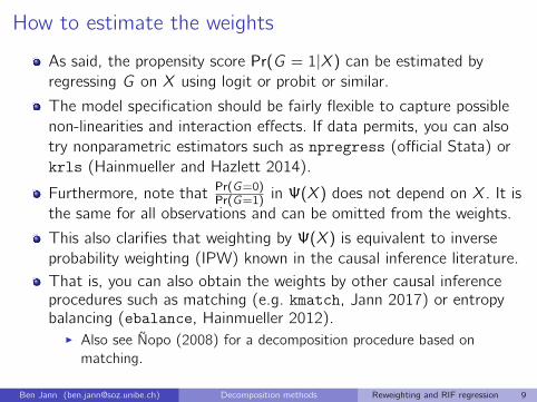
As said, the propensity score Pr(G = 1|X ) can be estimated byregressing G on X using logit or probit or similar.

The model specification should be fairly flexible to capture possiblenon-linearities and interaction effects. If data permits, you can alsotry nonparametric estimators such as npregress (official Stata) orkrls (Hainmueller and Hazlett 2014).

Furthermore, note that Pr(G=0)Pr(G=1) in Ψ(X ) does not depend on X . It is

the same for all observations and can be omitted from the weights.

This also clarifies that weighting by Ψ(X ) is equivalent to inverseprobability weighting (IPW) known in the causal inference literature.That is, you can also obtain the weights by other causal inferenceprocedures such as matching (e.g. kmatch, Jann 2017) or entropybalancing (ebalance, Hainmueller 2012).I Also see Ñopo (2008) for a decomposition procedure based onmatching.


LimitationsIf the sample is small, flexible estimation of the propensity score willnot be possible and the performance of the reweighting proceduremay be poor.A related problem is that in small samples common supportproblems are likely (observations for which the estimated propensityscore is close to zero or one); this can make the estimates unreliably(large variance in the weights).The effect of the weights is that they balance X between thegroups, i.e. the distribution of X in one group is adjusted to thedistribution of X in the other group. If the groups are very differentwith respect to X , this is hard to achieve. One consequence is againthat the weights will have a large variance (making estimatesimprecise). Furthermore, the desired balancing of X may be verypoor in such cases.It is thus always a good idea to check the balancing, like you woulddo in a matching analysis.



2 RIF regression


Example analysis. use gsoep29, clear(BCPGEN: Nov 12, 2013 17:15:52-251 DBV29). // selection. generate age = 2012 - bcgeburt. keep if inrange(age, 25, 55)(10,780 observations deleted). // compute gross wages and ln(wage). generate wage = labgro12 / (bctatzeit * 4.3) if labgro12>0 & bctatzeit>0(1,936 missing values generated). generate lnwage = ln(wage)(1,936 missing values generated). // X variables. generate schooling = bcbilzeit if bcbilzeit>0(318 missing values generated). generate ft_experience = expft12 if expft12>=0(15 missing values generated). generate ft_experience2 = expft12^2 if expft12>=0(15 missing values generated). generate public = oeffd12==1 if oeffd12>0(2,274 missing values generated). // summarize. summarize wage lnwage schooling ft_experience ft_experience2 public

Variable Obs Mean Std. Dev. Min Max

wage 8,090 16.26903 15.21083 .3624283 914.7287lnwage 8,090 2.615219 .5944705 -1.014929 6.818627

schooling 9,708 12.76118 2.73677 7 18ft_experie~e 10,011 13.41052 10.03473 0 39ft_experie~2 10,011 280.5277 324.8873 0 1521

public 7,752 .2582559 .4377037 0 1. marktouse touse lnwage schooling ft_experience ft_experience2 public(7388 observations marked)


Example analysis. sum lnwage if public==0 & touse, detail

lnwage

Percentiles Smallest1% .8439701 -1.0149295% 1.621675 -.447014110% 1.881213 -.3600028 Obs 5,47625% 2.230264 -.2954642 Sum of Wgt. 5,47650% 2.594971 Mean 2.5881

Largest Std. Dev. .607900575% 2.964234 5.22599690% 3.304779 5.42561 Variance .36954395% 3.50323 5.660272 Skewness -.280825999% 4.038553 6.818627 Kurtosis 5.460504. local prAVG = r(mean). local prD9D1 = r(p90)-r(p10). local prD9D5 = r(p90)-r(p50). local prD5D1 = r(p50)-r(p10). local prVar = r(Var). display exp(`prAVG')13.304465. display exp(`prD9D1')4.1518992. display exp(`prD9D5')2.033601. display exp(`prD5D1')2.0416489. display `prVar'.36954301


Example analysis. sum lnwage if public==1 & touse, detail

lnwage

Percentiles Smallest1% 1.472579 -.63763455% 1.989102 -.360002810% 2.219793 -.1856493 Obs 1,91225% 2.548718 .1803817 Sum of Wgt. 1,91250% 2.78988 Mean 2.749522

Largest Std. Dev. .451929675% 3.018445 4.06284690% 3.23959 4.067734 Variance .204240495% 3.394793 4.370919 Skewness -1.141899% 3.685552 5.287405 Kurtosis 9.000465. local puAVG = r(mean). local puD9D1 = r(p90)-r(p10). local puD9D5 = r(p90)-r(p50). local puD5D1 = r(p50)-r(p10). local puVar = r(Var). display exp(`puAVG')15.635162. display exp(`puD9D1')2.7726314. display exp(`puD9D5')1.5678569. display exp(`puD5D1')1.7684212. display `puVar'.20424037


Example analysis

. display exp(`prAVG' - `puAVG' )

.85093231

. display exp(`prD9D1' - `puD9D1')1.497458. display exp(`prD9D5' - `puD9D5')1.2970578. display exp(`prD5D1' - `puD5D1')1.1545037. display `prVar' - `puVar'.16530265


Example analysis. logit public c.schooling##c.ft_experience##c.ft_experience2 if touse, vsquishIteration 0: log likelihood = -4224.4285Iteration 1: log likelihood = -4096.5329Iteration 2: log likelihood = -4094.8721Iteration 3: log likelihood = -4094.8719Logistic regression Number of obs = 7,388

LR chi2(7) = 259.11Prob > chi2 = 0.0000

Log likelihood = -4094.8719 Pseudo R2 = 0.0307

public Coef. Std. Err. z P>|z| [95% Conf. Interval]

schooling .2096272 .0276666 7.58 0.000 .1554017 .2638528ft_experience .1109149 .1066695 1.04 0.298 -.0981534 .3199833c.schooling#

c.ft_experience -.009321 .0077856 -1.20 0.231 -.0245806 .0059385ft_experience2 -.0016162 .0075363 -0.21 0.830 -.016387 .0131547

c.schooling#c.ft_experience2 .0001383 .0005697 0.24 0.808 -.0009782 .0012548c.ft_experience#c.ft_experience2 -.0000484 .0001506 -0.32 0.748 -.0003436 .0002468

c.schooling#c.ft_experience#c.ft_experience2 4.62e-06 .0000117 0.39 0.694 -.0000184 .0000276

_cons -3.801943 .3974551 -9.57 0.000 -4.58094 -3.022945

. predict PS if e(sample), pr(2,638 missing values generated)


Example analysis. quietly two (kdens PS if public==0) (kdens PS if public==1), ///> xti("propensity score") legend(order(1 "private" 2 "public"))

0

5

10

15kd

ensi

ty P

S

0 .2 .4 .6 .8propensity score

privatepublic


Example analysis. summarize public if touse


public 7,388 .2587981 .4380041 0 1. local P_public = r(mean). generate PSI = (PS / `P_public') / ((1-PS) / (1 - `P_public')) if public==0 & touse(4,550 missing values generated). replace PSI = 1 if public==1 & touse(1,912 real changes made). summarize PSI if public==0 & touse


PSI 5,476 .9999512 .4742042 .2555806 4.334548. kdens PSI if public==0 & touse(bandwidth = .11136615)

0

.5

1

1.5

2

2.5

Density

0 1 2 3 4 5PSI


Example analysis. // Raw mean differences in covariates. tabstat PS schooling ft_experience ft_experience2 if touse, by(public) nototal ///> stat(mean var p10 p50 p90) columns(statistics)Summary for variables: PS schooling ft_experience ft_experience2

by categories of: publicpublic mean variance p10 p50 p90

0 .249332 .0060701 .1765754 .2183861 .371641512.63705 6.828291 10.5 11.5 1814.94805 98.56863 2 14 29321.9947 113321 4 196 841

1 .285909 .0086856 .1928914 .2541142 .432167513.77641 8.355398 10.5 13 1814.52866 101.5415 2 13.3 29312.5704 112618.3 4 176.89 841

. // Mean differens in weighted sample

. tabstat PS schooling ft_experience ft_experience2 [aw=PSI] if touse, by(public) nototal> ///> stat(mean var p10 p50 p90) columns(statistics)Summary for variables: PS schooling ft_experience ft_experience2

by categories of: publicpublic mean variance p10 p50 p90

0 .2858741 .0087147 .1937293 .2543135 .428788713.7805 8.523594 10.5 13 1814.55628 101.4321 1.9 13.2 29313.2988 112554.4 3.61 174.24 841

1 .285909 .0086856 .1928914 .2541142 .432167513.77641 8.355398 10.5 13 1814.52866 101.5415 2 13.3 29312.5704 112618.3 4 176.89 841


Example analysis. sum lnwage [aw=PSI] if public==0 & touse, detail

lnwage

Percentiles Smallest1% .9273517 -1.0149295% 1.704171 -.447014110% 1.942582 -.3600028 Obs 5,47625% 2.317276 -.2954642 Sum of Wgt. 5,475.732950% 2.69457 Mean 2.684965

Largest Std. Dev. .621130475% 3.071832 5.22599690% 3.409304 5.42561 Variance .38580395% 3.616559 5.660272 Skewness -.225696299% 4.245167 6.818627 Kurtosis 5.072671. local cAVG = r(mean). local cD9D1 = r(p90)-r(p10). local cD9D5 = r(p90)-r(p50). local cD5D1 = r(p50)-r(p10). local cVar = r(Var). display exp(`cAVG')14.657694. display exp(`cD9D1')4.3349997. display exp(`cD9D5')2.0436427. display exp(`cD5D1')2.1212122. display `c_Var'


Example analysis

. foreach s in AVG D9D1 D9D5 D5D1 Var {2. display %6s "`s': " "total difference = " %9.0g `pr`s'' - `pu`s'' ///

> " explained = " %9.0g `pr`s'' - `c`s''3. }

AVG: total difference = -.1614227 explained = -.0968657D9D1: total difference = .403769 explained = -.0431557D9D5: total difference = .2600985 explained = -.0049257D5D1: total difference = .1436706 explained = -.0382299Var: total difference = .1653026 explained = -.01626.. oaxaca lnwage schooling ft_experience ft_experience2, by(public) weight(1) nodetailBlinder-Oaxaca decomposition Number of obs = 7,388

Model = linearGroup 1: public = 0 N of obs 1 = 5476Group 2: public = 1 N of obs 2 = 1912

lnwage Coef. Std. Err. z P>|z| [95% Conf. Interval]

overallgroup_1 2.5881 .0082165 314.99 0.000 2.571996 2.604204group_2 2.749522 .0103413 265.88 0.000 2.729254 2.769791

difference -.1614227 .0132081 -12.22 0.000 -.18731 -.1355354explained -.0982116 .0089312 -11.00 0.000 -.1157164 -.0807068

unexplained -.0632111 .0118564 -5.33 0.000 -.0864493 -.0399729


Example analysis

. foreach s in AVG D9D1 D9D5 D5D1 Var {2. display %6s "`s': " "total difference = " %9.0g `pr`s'' - `pu`s'' ///

> " explained = " %9.0g `pr`s'' - `c`s''3. }

AVG: total difference = -.1614227 explained = -.0968657D9D1: total difference = .403769 explained = -.0431557D9D5: total difference = .2600985 explained = -.0049257D5D1: total difference = .1436706 explained = -.0382299Var: total difference = .1653026 explained = -.01626.. oaxaca lnwage schooling ft_experience ft_experience2, by(public) weight(1) nodetailBlinder-Oaxaca decomposition Number of obs = 7,388





unexplained -.0632111 .0118564 -5.33 0.000 -.0864493 -.0399729

Example analysis

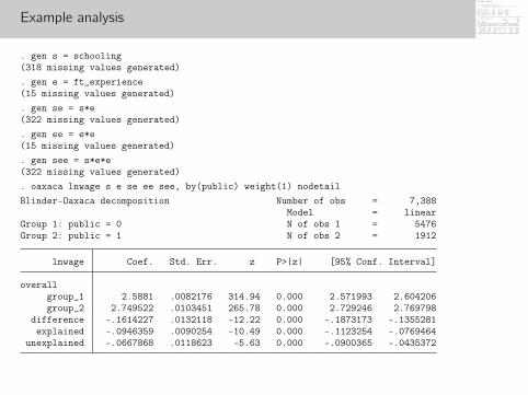
. gen s = schooling(318 missing values generated). gen e = ft_experience(15 missing values generated). gen se = s*e(322 missing values generated). gen ee = e*e(15 missing values generated). gen see = s*e*e(322 missing values generated). oaxaca lnwage s e se ee see, by(public) weight(1) nodetailBlinder-Oaxaca decomposition Number of obs = 7,388





unexplained -.0667868 .0118623 -5.63 0.000 -.0900365 -.0435372

. quietly two (kdens lnwage if public==0 & touse) ///> (kdens lnwage [aw=PSI] if public==0 & touse) ///> (kdens lnwage if public==1 & touse) ///> , legend(order(1 "private" 2 "adjusted private" 3 "public")) xti(lnwage)

0

.5

1

kden

sity

lnw

age

-2 0 2 4 6 8lnwage

privateadjusted privatepublic



2 RIF regression


Detailed decompositionFor binary covariates, a detailed decomposition of the contributionto the quantity effect can be obtained as follows.Let X1 be a binary and X2 be the vector of all other covariates. Acounterfactual distribution of Y in group 0, where the conditionaldistribution of X1 given the other covariate is changed to theconditional distribution of X1 in group 1, can be written as

FY 0|X 11(y) =

∫ ∫FY |X 0(y |X1,X2) dFX 1(X1|X2) dFX 0(X2)

=

∫ ∫FY |X 0(y |X1,X2)Ψ1(X1,X2) dFX 0(X1|X2) dFX 0(X2)

=

∫ ∫FY |X 0(y |X1,X2)Ψ1(X1,X2) dFX 0(X1,X2)

where

Ψ1(X1,X2) =dFX 1(X1|X2)

dFX 0(X1|X2)= X1

Pr1(X1 = 1|X2)

Pr0(X1 = 1|X2)+(1−X1)

Pr1(X1 = 0|X2)

Pr0(X1 = 0|X2)


Detailed decomposition

To compute Ψ1(X1,X2), regress X1 on X2 in separately group 0 andin group 1 using logistic regression or similar. Then replacePr0(X1 = 1|X2), Pr0(X1 = 0|X2), Pr1(X1 = 1|X2) andPr1(X1 = 0|X2) by predictions from these models.

A similar approach can also be used to determine the contribution ofa binary covariate to the structure component (see Fortin et al.2011).

For continuous covariates, things are less clear. One approachfollowed in the literature is to compute a series of reweightingdecompositions where the covariates are introduced one after theother. The problem with this approach is that results will be pathdependent.

A better approach is, for each covariate, to compute the contributionof the covariate while controlling for all other covariates.


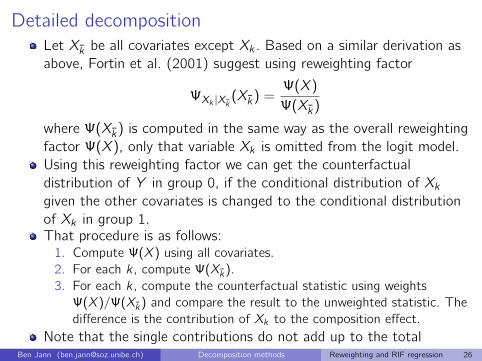
Detailed decompositionLet Xk̄ be all covariates except Xk . Based on a similar derivation asabove, Fortin et al. (2001) suggest using reweighting factor

ΨXk |Xk̄(Xk̄) =

Ψ(X )

Ψ(Xk̄)

where Ψ(Xk̄) is computed in the same way as the overall reweightingfactor Ψ(X ), only that variable Xk is omitted from the logit model.Using this reweighting factor we can get the counterfactualdistribution of Y in group 0, if the conditional distribution of Xkgiven the other covariates is changed to the conditional distributionof Xk in group 1.That procedure is as follows:1. Compute Ψ(X ) using all covariates.2. For each k , compute Ψ(Xk̄).3. For each k , compute the counterfactual statistic using weights

Ψ(X )/Ψ(Xk̄) and compare the result to the unweighted statistic. Thedifference is the contribution of Xk to the composition effect.

Note that the single contributions do not add up to the totalcomposition effect.Ben Jann ([email protected]) Decomposition methods Reweighting and RIF regression 26


2 RIF regression


Example analysis

. // schooling

. drop PS

. quietly logit public c.ft_experience##c.ft_experience2 if touse, vsquish

. predict PS if e(sample), pr(2,638 missing values generated). generate PSI_schooling = (PS / `P_public') / ((1-PS) / (1 - `P_public')) if public==0 &> touse(4,550 missing values generated). quietly sum lnwage [aw=PSI/PSI_schooling] if public==0 & touse, detail. local cAVGx = r(mean). local cD9D1x = r(p90)-r(p10). local cD9D5x = r(p90)-r(p50). local cD5D1x = r(p50)-r(p10). local cVarx = r(Var). foreach s in AVG D9D1 D9D5 D5D1 Var {

2. display %6s "`s': " "explained by schooling = " %9.0g `pr`s'' - `c`s'x'3. }

AVG: explained by schooling = -.1058771D9D1: explained by schooling = -.037792D9D5: explained by schooling = -.0082781D5D1: explained by schooling = -.0295138Var: explained by schooling = -.0123014


Example analysis

. // experience

. drop PS

. quietly logit public schooling if touse, vsquish

. predict PS if e(sample), pr(2,638 missing values generated). generate PSI_experience = (PS / `P_public') / ((1-PS) / (1 - `P_public')) if public==0 &> touse(4,550 missing values generated). quietly sum lnwage [aw=PSI/PSI_experience] if public==0 & touse, detail. local cAVGx = r(mean). local cD9D1x = r(p90)-r(p10). local cD9D5x = r(p90)-r(p50). local cD5D1x = r(p50)-r(p10). local cVarx = r(Var). foreach s in AVG D9D1 D9D5 D5D1 Var {

2. display %6s "`s': " "explained by experience = " %9.0g `pr`s'' - `c`s'x'3. }

AVG: explained by experience = -.0051177D9D1: explained by experience = .0166521D9D5: explained by experience = .01406D5D1: explained by experience = .0025921Var: explained by experience = .0081723


Example analysis

. oaxaca lnwage schooling (experience: ft_experience ft_experience2), by(public) weight(1)Blinder-Oaxaca decomposition Number of obs = 7,388





unexplained -.0632111 .0118564 -5.33 0.000 -.0864493 -.0399729

explainedschooling -.1100746 .0078852 -13.96 0.000 -.1255293 -.0946199experience .011863 .0059652 1.99 0.047 .0001714 .0235545

unexplainedschooling .3844041 .0573983 6.70 0.000 .2719055 .4969026experience .0522172 .0253538 2.06 0.039 .0025247 .1019097

_cons -.4998323 .0645484 -7.74 0.000 -.6263449 -.3733197

experience: ft_experience ft_experience2



2 RIF regression


Exercise 7

Rerun the above analysis (without the detailed decomposition tosave time), but use a different counterfactual (distribution of publicsector wages if X is adjusted to the private sector).

Furthermore, wrap the analysis into a program and apply thebootstrap to compute standard errors and confidence intervals.



2 RIF regression


Influence functionsA very nice approach to compute Oaxaca-Blinder typedecompositions for almost any distributional statistic of interest isbased on influence functions.An influence functions is a function that quantifies how a targetstatistic changes in response to small changes in the data. That is,for each value y , the influence function IF(y ; ν,FY ) provides anapproximation of how the functional ν(FY ) changes if a smallprobability mass is added at point y .Influence functions are used in robust statistics to describe therobustness properties of various statistic (a robust statistic has abounded influence function).There is also a close connection to the sampling variance of astatistic. The asymptotic sampling variance of a statistic is equal tothe sampling variance of the mean of the influence function.Therefore, influence functions provide an easy way to estimatestandard errors for many statistics (e.g. inequality measured).


RIF regressionFor example, the influence function of quantile Qp is simply

IF(y ; Qp,FY ) =p − I (y ≤ Qp)

fY (Qp)

Influence functions are centered around zero (that is, have anexpected value of zero). To center an influence function around thestatistic of interest, we can simply add the statistic to the influencefunction. This is called a recentered influence function

RIF(y ; ν,FY ) = ν(FY ) + IF(y ; ν,FY )

The idea now is to model the conditional expectation ofRIF(y ; ν,FY ) using regression models, e.g. using a linear model

E(RIF(Y ; ν,FY )|X ) = Xγ

Coefficient γ thus provides an approximation of how ν(FY ) reacts tochanges in X .


RIF regression decomposition

In practice, taking the example of a quantile, we would first computethe sample quantile Q̂p and then use kernel density estimation to getf̂ (Q̂p), the density of Y at point Q̂p.

RIF(Yi ; Qp,FY ) is then computed for each observation by pluggingthese estimates in to the above formula.

Finally, we regress RIF(Yi ; Qp,FY ) on X to get an estimate of γ.

Using the coefficients from RIF regression in two groups, we canperform an Oaxaca-Blinder type decomposition for Qp. For example:

∆̂Qp = ∆̂QpX + ∆̂

QpS = (X̄ 0 − X̄ 1)γ̂0 + X̄ 1(γ̂0 − γ̂1)

A similar procedure can be followed for any other statistic ν(FY ). Allyou have to know is the influence function, which is usually easy tofind in the statistical literature.


RIF regression decomposition

Command rifreg provides RIF regression for quantiles, the Ginicoefficient, and the variance. It can be obtained fromhttps://economics.ubc.ca/faculty-and-staff/nicole-fortin/.

The RIF variables stored by rifreg can then be used in oaxaca.


https://economics.ubc.ca/faculty-and-staff/nicole-fortin/

Example analysis

. rifreg lnwage schooling ft_experience ft_experience2 if public==0 & touse, variance reta> in(RIF)(4,550 missing values generated)

Source SS df MS Number of obs = 5476F( 3, 5472) = 21.01

Model 37.9668705 3 12.6556235 Prob > F = 0.0000Residual 3296.44132 5472 .602419832 R-squared = 0.0114

Adj R-squared = 0.0108Total 3334.40819 5475 .609024327 Root MSE = .77616

RIF Coef. Std. Err. t P>|t| [95% Conf. Interval]

schooling .0226022 .0040773 5.54 0.000 .014609 .0305954ft_experience -.014324 .0038439 -3.73 0.000 -.0218596 -.0067885ft_experience2 .0002986 .0001136 2.63 0.009 .0000758 .0005214

_cons .201826 .0589913 3.42 0.001 .0861797 .3174723

. regress RIF schooling ft_experience ft_experience2, noheader

RIF Coef. Std. Err. t P>|t| [95% Conf. Interval]

schooling .0226022 .0040773 5.54 0.000 .014609 .0305954ft_experience -.014324 .0038439 -3.73 0.000 -.0218596 -.0067885ft_experience2 .0002986 .0001136 2.63 0.009 .0000758 .0005214

_cons .201826 .0589913 3.42 0.001 .0861797 .3174723


Example analysis. scatter RIF lnwage. drop RIF

0

5

10

15

20

RIF

-2 0 2 4 6lnwage


Example analysis. quietly rifreg lnwage if public==0 & touse, variance retain(RIFprivate). quietly rifreg lnwage if public==1 & touse, variance retain(RIFpublic). gen RIF = cond(public==1, RIFpublic, RIFprivate)(2,638 missing values generated). oaxaca RIF schooling (experience: ft_experience ft_experience2), by(public) weight(1)Blinder-Oaxaca decomposition Number of obs = 7,388


RIF Coef. Std. Err. z P>|z| [95% Conf. Interval]

overallgroup_1 .3694755 .0105488 35.03 0.000 .3488003 .3901508group_2 .2041335 .0132183 15.44 0.000 .1782262 .2300409

difference .165342 .0169115 9.78 0.000 .132196 .198488explained -.0289454 .0052513 -5.51 0.000 -.0392378 -.0186531

unexplained .1942874 .0174656 11.12 0.000 .1600555 .2285194

explainedschooling -.025752 .0049448 -5.21 0.000 -.0354436 -.0160605experience -.0031934 .0015953 -2.00 0.045 -.0063201 -.0000667

unexplainedschooling .34344 .0852943 4.03 0.000 .1762663 .5106137experience .0831629 .0376505 2.21 0.027 .0093693 .1569565

_cons -.2323155 .0959429 -2.42 0.015 -.4203601 -.0442708

experience: ft_experience ft_experience2


Limitations

Effects on the RIF of statistics such as inequality measures are likelyto be highly nonlinear. Interaction effects are also likely.

It is therefore important to use a flexible model specification.

In case of interaction effects this again limits the usefulness of theprocedure for obtaining detailed decompositions.


References

Chernozhukov, Victor, Iván Fernández-Val, Blaise Melly (2013). Inference onCounterfactual Distributions. Econometrica 81(6):2205–2268.

DiNardo, John E., Nicole Fortin, Thomas Lemieux (1996). Labour MarketInstitutions and the Distribution of Wages, 1973-1992: A SemiparametricApproach. Econometrica 64(5):1001–1046.

Firpo, Sergio, Nicole Fortin, Thomas Lemieux (2007). Decomposing WageDistributions using Recentered Influence Function Regressions. Working paper.

Firpo, Sergio, Nicole M. Fortin, Thomas Lemieux (2009). Unconditional QuantileRegressions. Econometrica 77:953–973.

Hainmueller, Jens (2012). Entropy Balancing: A Multivariate ReweightingMethod to Produce Balanced Samples in Observational Studies. Political Analysis20(1):25–46.

Hainmueller, Jens, Chad Hazlett (2014). Kernel Regularized Least Squares:Reducing Misspecification Bias with a Flexible and Interpretable MachineLearning Approach. Political Analysis 22(2):143–168.


References

Jann, Ben (2017). kmatch: Stata module for multivariate-distance andpropensity-score matching. Available fromhttp://ideas.repec.org/c/boc/bocode/s458346.html.

Juhn, Chinhui, Kevin M. Murphy, Brooks Pierce (1993). Wage Inequality and theRise in Returns to Skill. Journal of Political Economy 101(3):410–442.

Machado, José A. F., José Mata (2005). Counterfactual decomposition ofchanges in wage distributions using quantile regression. Journal of AppliedEconometrics 20(4):445–465.

Melly, Blaise (2005). Decomposition of differences in distribution using quantileregression. Labour Economics 12(4):577–590.

Melly, Blaise, 2006. Estimation of counterfactual distributions using quantileregression. University of St. Gallen, Discussion Paper.

Ñopo, Hugo (2008). Matching as a Tool to Decompose Wage Gaps. The Reviewof Economics and Statistics 90:290–299.


http://ideas.repec.org/c/boc/bocode/s458346.html

Documents

Decomposition methods in the social sciences - Bamberg … · Decompositionmethodsinthesocialsciences BambergGraduateSchoolofSocialSciences,June7–8,2018 BenJann University of Bern,