Embed Size (px)
Citation preview

HAL Id: hal-00585717https://hal.archives-ouvertes.fr/hal-00585717
Preprint submitted on 13 Apr 2011
HAL is a multi-disciplinary open accessarchive for the deposit and dissemination of sci-entific research documents, whether they are pub-lished or not. The documents may come fromteaching and research institutions in France orabroad, or from public or private research centers.
L’archive ouverte pluridisciplinaire HAL, estdestinée au dépôt et à la diffusion de documentsscientifiques de niveau recherche, publiés ou non,émanant des établissements d’enseignement et derecherche français ou étrangers, des laboratoirespublics ou privés.
Decomposing Logical Relations with ForcingGuilhem Jaber, Nicolas Tabareau
To cite this version:
Guilhem Jaber, Nicolas Tabareau. Decomposing Logical Relations with Forcing. 2011. hal-00585717

Decomposing Logical Relations with Forcing
Guilhem Jaber
ENS Cachan
Nicolas Tabareau
INRIA
Abstract
Logical relations have now the maturity to deal with pro-gram equivalence for realistic programming languages withfeatures likes recursive types, higher-order references andfirst-class continuations. However, such advanced logicalrelations—which are defined with technical developmentslike step-indexing or heap abstractions using recursively de-fined worlds—can make a proof tedious. A lot of work hasbeen done to hide step-indexing in proofs, using Godel-Lob logic. But to date, step-indexes have still to appearexplicitely in particular constructions, for instance whenbuilding recursive worlds in a stratified way. In this paper,we go one step further, proposing an extension of Abadi-Plotkin logic with forcing construction which enables to en-capsulate reasoning about step-indexing or heap in differentlayers. Moreover, it gives a uniform and abstract manage-ment of step-indexing for recursive terms or types and forhigher-order references.
1. Introduction
1.1 Logical relations
Logical relations appear in the last decade to be a power-ful technique for proving program equivalence, able to dealwith concrete non-trivial equivalence of programs makinguse of complex features like recursive types, control opera-tors and higher-order references. For instance, it is now wellknown that fix point operators or recursive types [1] canbe handled by logical relations using step indexing, a tech-nique introduced in [3]. To avoid the apparent circularity inthe definition of logical relations for recursive types, step-indexes are used to stratify logical relations with a naturalnumber representing roughly the number of steps for whichthe programs in question behave similarly. In this way, it be-comes possible to prove the equivalence of many programsthat makes use of recursive types by performing a simpleinduction on step-indexes. But the management of step in-dexes during a proof appears to be—borrowing a word fromN. Benton—”ugly”. That’s why many authors, starting fromthe work of A. Appel et al. [4], have proposed to hide step-indexing using Godel-Lob logic.
[Copyright notice will appear here once ’preprint’ option is removed.]
More recently, D. Dreyer et al. [2, 12] have defined step-indexed Kripke logical relations with the ability to establishproperties about local state that evolve during computationin some controlled fashion. Basically, instead of using localinvariants as in the seminal work of A. Pitts and I. Stark [17],the evolution of the heap is constrained by a state transitionsystem (STS).
To encompass higher-order references, D. Dreyer et al.have to extend their notion of heap relations that are usedin each node of the STSs of a world to heap relations takinga world as a parameter. While all those ideas appear to beintuitively very elegant, their precise definitions still requiresto make an explicit use of step-indexing and stratificationwhere people just would like to use Godel-Lob logic andrecursively defined set of worlds.
This paper proposes a logical setting where all thosedifferent notions can be defined modularly and combineduniformly.
1.2 Forcing for set theory
Forcing is a method originally designed by P. Cohen in the60s to prove the independence of the Continuum Hypothesisfrom the axiomatic set theory ZFC [8]. The main idea is toextend a ground model M to a new model M [G] by addinga new generic element G to M . As M [G] is in general re-ally complicated, P. Cohen has proposed to control the truepropositions in M [G] by translating them into M . To do so,he has used forcing conditions, which have to be seen as ap-proximations of G. Such forcing conditions live in M whileit is not the case for the generic element G. Thus, from a for-mula ϕ of M [G], the idea is to build syntactically a formulap ϕ—pronounced “p forces ϕ”—that lives in M , and suchthat ϕ will be true when there is a“correct”approximation pof G such that p ϕ in M . One key property of forcing con-ditions is that they are ordered. Intuitively, p ≤ q when p isa more precise approximation of G than q, i.e. contains moreinformation, so the relation has to be monotonous for thisorder. In a similar manner, J.-L. Krivine has used forcingto transform into a program any proof using the dependentchoice axiom and the existence of a non-trivial ultrafilteron N [14]. This approach has recently been clarified by A.Miquel [16], who tries to understand proof transformationinduced by forcing translation through Curry-Howard iso-morphism. Finally, in [9], forcing is used to prove construc-tively the uniform continuity of some functionals defined inintuitionistic type theory. In this article, we do not pretendto follow precisely the line drawn by those works, but ratheran alternative line promoting the general slogan:
”Forcing can be used to add logical principles modularly.”
This slogan will be illustrated by defining logical relations indifferent logic layers having more and more logical principles.
1 2011/3/30

1.3 Approximating logical relations with forcingconditions
In analogy to Cohen’s forcing, we advocate that forcing con-ditions in the setting of logical relations can be used to ap-proximate the notion of observation. This follows the well-known fact that step-indexing can be seen as an approxima-tion of the equitermination observation O(t1, t2) which saysthat the term t1 terminates if and only if t2 terminates.
More precisely, suppose given a logic in which logicalrelations can be expressed and consider the formula
E JUnit → UnitK (t1, t2)
that says that the two terms t1 and t2 are related at typeUnit → Unit. In presence of complex features in the lan-guage, we sometimes want to be able to relate terms thatare not absolutely equivalent but only under some conditionp, written
p E JUnit → UnitK (t1, t2).
Technically, the formula above is translated into a formula ofthe ground logic where the forcing condition p goes throughthe formula monotonically until the observation
p O(t1, t2)
which approximates the original observation. For instance,when the forcing condition is a world w, the approximatedobservation says that t1 and t2 behave the same for all heapsrelated by w. When the forcing condition is a step-index n,the approximated observation says that t1 and t2 behave thesame for n steps.
1.4 Step-indexing as forcing conditions
As indicated above, step-indexes can be rephrased as forcingconditions over integers (with the usual order) that approx-imate the observation. In this way, it is possible to recoveruniformly many definitions given in previous works. But thereally interesting part is that we can formalize the logicalprinciples that step-indexing validate in the forcing layer.
Forcing conditions can be used to approximate existingformulas but also to give some meaning to new connector inthe logic. Namely, in the step-indexed (SI) layer, one candefine the so-called “later” operator as
n ⊲ϕdef= ∀m < n, m ϕ
and show that the Lob rule is valid under forcing. To bemore abstract about step-indexes, let us make explicit thelogic associated to the forcing layer
ψ1, . . . , ψk ⊢SI ϕdef= ∀n, (n ψ1, . . . , n ψk) ⊢ (n ϕ)
that is, ϕ is true in the SI layer if and only if it is forcedby any step-index. This formalizes the intuition that step-indexing provides approximations of logical relations whoselimits are logical relation themselves. In the SI layer, theLob rule is also valid and can simply be expressed by
⊲P ⊢SI P
⊢SI P
This means that working in the SI layer equipped theground logic with an induction principle for free. But we willsee in Section 4 that the SI layer has much more logical prin-ciples, for instance the ability to define logical relations orworlds recursively without making any explicit use of strat-ification. But the fact that each new formula is translatedin the previous layer using the forcing relation enables to
validate the new reasoning principles in the previous layer,which means that:
”The consistency of the logic defined in a forcing layerensues from the consistency of the ground logic.”
The idea of using forcing to prove relative consistency resultsin proof theory is not new, see for example [5], but here, weapply it to type theory.
While step-indexing is fitted to reason on contextualapproximations, it is harder to design step-indexed logicalrelations to reason on contextual equivalences. In [11], thenrefined in [13], a method based on a direction variable isgiven, which corresponds in our framework to a simpleforcing with only two conditions l, r.
1.5 Kripke worlds as forcing conditions
Turning back to the seminal work of A. Pitts and I.Stark [17], let us consider forcing conditions over a set ofworlds defined by
Worlddef= Heap×Heap → Prop
A world is thus a relation that states which heaps are inrelation in this world. A world w′ is in the future of a worldw (noted w′ ⊒ w) when w′ extends w on new locations.Then, defining the relation Ow as t1 and t2 behave the samefor all heaps related by w, we can recover the usual definitionof Kripke logical relations (see Section 5 for details). Notethat the judgement
w ϕ
was already present in the work of A. Appel et al. [4], as thedefinition of Kripke model, for which truth is not absolutebut relative to some appropriate notion of world.
As far as higher order references are concerned, we can nolonger define worlds in this simple manner since referencescan point to other references whose relation depends on theworld. So one would like to define world recursively as
Worlddef= (Heap×Heap) → World → Prop
However, by a cardinality argument, there is no solution tothis equation in Set. This has lead many authors (see [4]or [12], for instance) to work with a stratified approximatedsolution to this equation. But it seems that step-indexingis coming into the picture again. Indeed, in [4] or [12],worlds are indexed by an integer that decreases when timeadvances.
One of the main contributions of this paper is to showthat this stratified construction can be recovered by definingworlds in the step-indexed (SI) layer, using directly thepossibility to define recursive kinds.
2. The Logic FLR
2.1 The language Fµ!
We consider the language Fµ!; a standard call-by-value λ-calculus with a fixpoint construction, recursive types, uni-versal polymorphism, and ML-like references. For simplicity,we do not have products, sums or existential types, but theycould be added easily following [13]. The syntax and the op-erational semantics are given in in Figure 1, while the typingrules can be found in Appendix.
2.2 Contextual equivalence
Let ∆ be a context for the free type variables, Υ for thelocations used by the term, and Γ for the free term variables.
2 2011/3/30

τ, σdef= Unit | Nat | α | τ → σ | ∀α.τ | µα.τ | ref τ
vdef= () | n | l | λx.M | fix f(x).M | Λα.M | roll v
(where n ∈ Nat, l ∈ Loc)
M,Ndef= v | x | τ | MN | rollM | unrollM | refM |
!M | M := N
Kdef= | KM | Kτ | vK | rollK | unrollK |
refK | !K | K :=M | v := K
hdef= emp | h[l 7→ v] | h • [l 7→ v]
((λx.M)v, h) 7→ (M v/x , h)(fix f(x).M)v, h) 7→ (M v/x fix f(x).M/f , h)
((Λα.M)τ, h) 7→ (M τ/α , h)(unroll (rollM), h) 7→ (M,h)
(!l, h) 7→ (v, h) when h(l) = v(ref v, h) 7→ (l, h • [l 7→ v]) with l /∈ dom(h)
(l := v, h) 7→ ((), h[l 7→ v]) when l ∈ dom(h)
(M1, h1) 7→ (M1, h2)
(K[M1], h1) 7→ (K[M2], h2)
Figure 1. Definitions of Fµ!
Contexts C are defined as terms with a hole [.] anywherein the term, and have a type ⊢ C : (∆;Υ; Γ ⊢ τ) →(∆′; Υ′; Γ′ ⊢ σ) saying that for any M with ∆;Υ; Γ ⊢M : τ ,we have ∆′; Υ′; Γ′ ⊢ C[M ] : σ. The typing rules of contextare usual and can be found for example in the additionaldetails of [11]. The contextual equivalence M1 ≃ctx M2 : τis then defined over arbitrary context C with a hole:
M1 ≃∆;Υ;Γctx M2 : τ
means that ∆;Υ; Γ ⊢ M1,M2 : τ and for all contexts C(such that ⊢ C : (∆;Υ; Γ ⊢ τ) → (∆′; Υ′; Γ′ ⊢ σ)), C[M1]and C[M2] equiterminate.
2.3 Syntax of FLR
Unlike Abadi-Plotkin logic [18] and all the successive de-velopments like LSLR and LADR, which are based onsecond-order logic, we use higher-order logic. The resultinglogic, called FLR, constitutes a language in which logicalrelations—and their extension using a forcing condition—can be defined.
FLR is an extension of (Curry style) Fω with implicit de-pendent types and a constructor for finite partial functions.We call kinds the types of the logic, to be differentiated fromtypes of Fµ!. Kinds are defined as :
T, U := Natp | Loc | Term | Val | Cont | Type | Prop | τ |⊤ | ⊥ | T × U | T → U | T →fin U | ∀x : T.U
where p ∈ N. Cont will be the kind of contexts, while Typewill be the kind of types of Fµ!.
The atomic propositions are: (1) M = N : syntacti-cal equality on terms, locations and heaps; (2) (M,h1) →(N,h2): reduction relation on pairs of term and heap; (3)abstract notion of observation O on pairs of term and heap;(4) left and right approximations of the observation Ol
n,Orn.
The idea is that Oln,O
rn are approximations of O, controlled
by the forcing conditions. Dealing with equitermination, Oln
will represent the left approximation for at most n steps, i.e.
“Oln((t1, h1), (t2, h2)) iff for all k ≤ n, if (t1, h1) can be
reduced k times then (t2, h2) terminates.”
It is axiomatized by the logical rules given in Section 2.4.Formulas are defined by :
P,Q := n | l | M | K | τ | O | Oln | Or
n | M = N |(M,h1) → (N,h2) | P ∧Q | P ∨Q |P ⇒ Q | ∀x : T.P | ∃x : T.P | (x).P |π1P | π1Q | 〈P,Q〉 | P ∈ Q
In the following, C denotes a logical context P , i.e. a listof propositions used as hypothesis, while Γ will be a typingcontext. We abbreviateQ ∈ P as P (Q). The well-formednessof propositions is ensured by standard typing rules given inFigure 2.
2.4 Inference rules of FLR
Our logic comes with a congruence ∼= on formulas, whichtake into account β and η equality. It is defined as thesmallest congruence satisfying the following axioms :
t ∈ x.P ∼= P t/xx.(x ∈ P ) ∼= P when x /∈ FV (P )π1 〈P,Q〉 ∼= Pπ2 〈P,Q〉 ∼= Q
There are also inference rules describing the reduction ofFµ!, mimicking the operational semantics of Figure 1.
FLR is equipped with standard inference rules given inFigure 3. Approximated observation relations Ol
n and Orn
satisfy specific inference rules (we only present the rules forl):
Γ; C ⊢ Olk((M1, h1), (M2, h2) Γ; C ⊢ k < n
Γ; C ⊢ Oln((M1, h1), (M2, h2))
Γ; C ⊢ (M1, h1) → (M ′
1, h′
1)
Γ; C ⊢ ∀k < n.Olk((M
′
1, h′
1), (M2, h2))
Γ; C ⊢ Oln((M1, h1), (M2, h2))
Note that in the ground logic, there is no need for inferencerules for O. The expected inference rules will appear whenworking in the step-indexed forcing layer.
The coherence of FLR can be ensured by constructing amodel adapted from the coherent space model of Miquel [15].Our logic is just a fragment of its logic (without universesand dependent types) with the additional presence of ⊤, ‚and Natp base sorts.
2.5 Partial finite function
To model heaps and world, we will need partial functionswith finite support as we must guarantee to have free spacein the heap1. That is Heap must be defined as Loc →fin Val.
We use the kind A→fin B of partial finite functions fromA to B, a predicate dom on them, plus the empty functionemp and two constructors f • g and [u 7→ v]. We also havea constructor f [u 7→ v] which enables to change the value ofa partial function f .
The usual typing rules are given in Annexe and the logicalrules are:
Γ; C ⊢ u /∈ dom(f)
Γ; C ⊢ (f • [u 7→ v])(u) = v
Γ; C ⊢ u ∈ dom(f)
Γ; C ⊢ (f [u 7→ v])(u) = v
1 It seems to be possible to encode them in our logic, like in [19],but we prefer to define them directly in our system.
3 2011/3/30

q ≤ p
Γ ⊢ q : Natp Γ ⊢M : Term Γ ⊢ v : Val Γ ⊢ K : Cont Γ ⊢ l : Loc Γ ⊢ τ : Type Γ ⊢ P : ⊤
Γ, x : ⊥ ⊢ P : T for any P
(x : T ) ∈ Γ
Γ ⊢ x : T
Γ, x : T ⊢ P : U
Γ ⊢ x.P : T → U
Γ ⊢ P : T → U Γ ⊢ Q : T
Γ ⊢ Q ∈ P : U
Γ ⊢ P : T × U
Γ ⊢ π1P : T
Γ ⊢ P : T × U
Γ ⊢ π2P : U
Γ ⊢ P : T Γ ⊢ Q : U
Γ ⊢ 〈P,Q〉 : T × U
Γ ⊢ P : T Γ ⊢ T <: U
Γ ⊢ P : U
Γ, x : T ⊢ P : U
Γ ⊢ P : ∀x : T.U
Γ ⊢ P : Prop Γ ⊢ Q : Prop
Γ ⊢ P ⇒ Q : Prop
Γ ⊢ P : Prop Γ ⊢ Q : Prop
Γ ⊢ P ∧Q : Prop
Γ ⊢ P : Prop Γ ⊢ Q : Prop
Γ ⊢ P ∨Q : Prop
Γ, x : T ⊢ P : Prop
Γ ⊢ ∀x : T.P : Prop
Γ, x : T ⊢ P : Prop
Γ ⊢ ∃x : T.P : Prop
Γ ⊢M1,M2 : Term Γ ⊢ h1, h2 : Heap
Γ ⊢ O((M1, h1), (M2, h2)) : Prop
Γ ⊢M1,M2 : Term Γ ⊢ h1, h2 : Heap
Γ ⊢ (M1, h1) 7→ (M2, h2) : Prop
Γ ⊢M1,M2
Γ ⊢M1 =M2 : Prop
Γ ⊢ h1, h2 : Heap
Γ ⊢ h1 = h2 : Prop
Figure 2. Typing rules of FLR
P ∈ C
Γ; C ⊢ P
Γ; C ⊢ P ⇒ Q Γ; C ⊢ P
Γ; C ⊢ Q
Γ; C, P ⊢ Q
Γ; C ⊢ P ⇒ Q
Γ; C ⊢ P P ∼= P ′
Γ; C ⊢ P ′ Γ, q : Natp; C ⊢ q ≤ p
Γ; C ⊢ P Γ; C ⊢ Q
Γ; C ⊢ P ∧Q
Γ; C ⊢ P ∧Q
Γ; C ⊢ P
Γ; C ⊢ P ∧Q
Γ; C ⊢ Q
Γ; C ⊢ P
Γ; C ⊢ P ∨Q
Γ; C ⊢ Q
Γ; C ⊢ P ∨Q
Γ; C ⊢ P ∨Q Γ; C, P ⊢ R Γ; C, Q ⊢ R
Γ; C ⊢ R
Γ, x : T ; C ⊢ P x /∈ C
Γ; C ⊢ ∀x : T.P
Γ; C ⊢ ∀x : T.P Γ ⊢ t : T
Γ; C ⊢ P t/x
Γ; C ⊢ P t/x
Γ; C ⊢ ∃x : T.P
Γ; C ⊢ ∃x : T.P Γ, t : T ; C, P t/x ⊢ Q
Γ; C ⊢ Q
Figure 3. Basic Logical rules of FLR
plus the usual commutativity and associativity equality onthe two constructors • and [u 7→ v], extending the congru-ence ∼=.
2.6 Subtyping
To eliminate implicit dependent types, we use a standardsubtyping relation that is a preorder, is covariant in botharguments of the product types and validates the inferencerules of Figure 4. Even if a rule like ⊤ → ⊤ <: ⊤ couldappear to be non-standard, one can check that it is satisfiedin the slightly adapted model of [15].
2.7 Logical relations
We can already build a logical relation in this logic for thepure, polymorphic fragment of Fµ!. Logical relations, builtby induction on types and defined on the following kinds
Reldef= (Term×Term) → Prop , Relτ,σ
def= (τ × σ) → Prop
are given in Figure 5. The definition of logical relations forpolymorphic types uses an environment η which maps freetypes to relations. It is important to notice that the defini-tion of E JτK is made by biorthogonality, which is central inour work since it is the only place where the observation Oappears. Note that for the definitions of S JΥK and ≃log, we
Γ ⊢ T <: ⊤ Γ ⊢ ⊤ → ⊤ <: ⊤
q ≤ p
Γ ⊢ Natq <: Natp
Γ ⊢ Natp <: Nat
Γ ⊢ T <: T ′ Γ ⊢ U <: U ′
Γ ⊢ T × U <: T ′ × U ′
Γ ⊢ T ′ <: T Γ ⊢ U <: U ′
Γ ⊢ T → U <: T ′ → U ′
Γ ⊢ t : T
Γ ⊢ ∀x : T.U <: U t/x
Γ ⊢ T ′ <: T Γ, x : T ′ ⊢ U <: U ′
Γ ⊢ ∀x : T.U <: ∀x : T ′.U ′
Figure 4. Subtyping rules
anticipate Section 5 and use the logical relation on referencetypes.
3. Forcing layers
To increase the power of our logic, we will extend it with newconstructions, and new reasoning principles (e.g. the Lob
4 2011/3/30
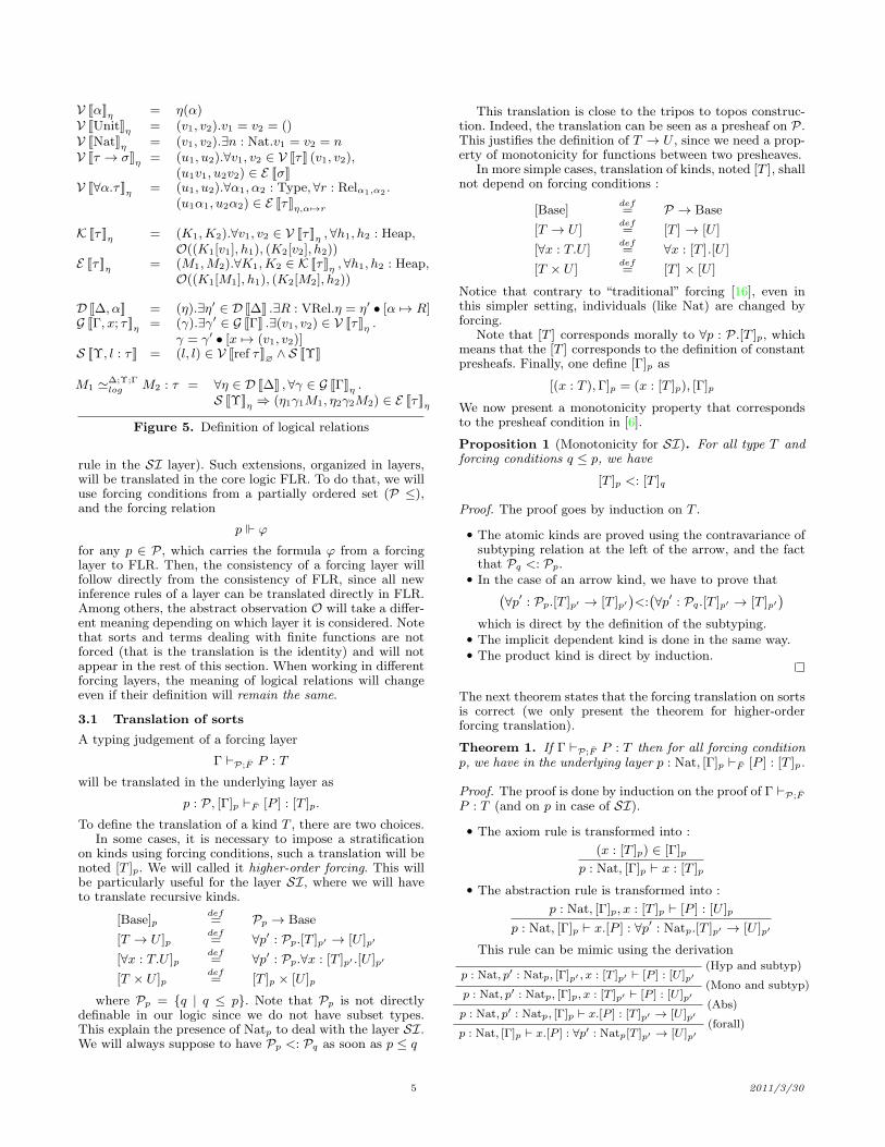
V JαKη = η(α)V JUnitKη = (v1, v2).v1 = v2 = ()V JNatKη = (v1, v2).∃n : Nat.v1 = v2 = nV Jτ → σKη = (u1, u2).∀v1, v2 ∈ V JτK (v1, v2),
(u1v1, u2v2) ∈ E JσKV J∀α.τKη = (u1, u2).∀α1, α2 : Type, ∀r : Relα1,α2
.(u1α1, u2α2) ∈ E JτKη,α 7→r
K JτKη = (K1,K2).∀v1, v2 ∈ V JτKη , ∀h1, h2 : Heap,O((K1[v1], h1), (K2[v2], h2))
E JτKη = (M1,M2).∀K1,K2 ∈ K JτKη , ∀h1, h2 : Heap,O((K1[M1], h1), (K2[M2], h2))
D J∆, αK = (η).∃η′ ∈ D J∆K .∃R : VRel.η = η′ • [α 7→ R]G JΓ, x; τKη = (γ).∃γ′ ∈ G JΓK .∃(v1, v2) ∈ V JτKη .
γ = γ′ • [x 7→ (v1, v2)]S JΥ, l : τK = (l, l) ∈ V Jref τK
∅∧ S JΥK
M1 ≃∆;Υ;Γ
log M2 : τ = ∀η ∈ D J∆K , ∀γ ∈ G JΓKη .S JΥKη ⇒ (η1γ1M1, η2γ2M2) ∈ E JτKη
Figure 5. Definition of logical relations
rule in the SI layer). Such extensions, organized in layers,will be translated in the core logic FLR. To do that, we willuse forcing conditions from a partially ordered set (P ≤),and the forcing relation
p ϕ
for any p ∈ P, which carries the formula ϕ from a forcinglayer to FLR. Then, the consistency of a forcing layer willfollow directly from the consistency of FLR, since all newinference rules of a layer can be translated directly in FLR.Among others, the abstract observation O will take a differ-ent meaning depending on which layer it is considered. Notethat sorts and terms dealing with finite functions are notforced (that is the translation is the identity) and will notappear in the rest of this section. When working in differentforcing layers, the meaning of logical relations will changeeven if their definition will remain the same.
3.1 Translation of sorts
A typing judgement of a forcing layer
Γ ⊢P;F P : T
will be translated in the underlying layer as
p : P, [Γ]p ⊢F [P ] : [T ]p.
To define the translation of a kind T , there are two choices.In some cases, it is necessary to impose a stratification
on kinds using forcing conditions, such a translation will benoted [T ]p. We will called it higher-order forcing. This willbe particularly useful for the layer SI, where we will haveto translate recursive kinds.
[Base]pdef= Pp → Base
[T → U ]pdef= ∀p′ : Pp.[T ]p′ → [U ]p′
[∀x : T.U ]pdef= ∀p′ : Pp.∀x : [T ]p′ .[U ]p′
[T × U ]pdef= [T ]p × [U ]p
where Pp = q | q ≤ p. Note that Pp is not directlydefinable in our logic since we do not have subset types.This explain the presence of Natp to deal with the layer SI.We will always suppose to have Pp <: Pq as soon as p ≤ q
This translation is close to the tripos to topos construc-tion. Indeed, the translation can be seen as a presheaf on P.This justifies the definition of T → U , since we need a prop-erty of monotonicity for functions between two presheaves.
In more simple cases, translation of kinds, noted [T ], shallnot depend on forcing conditions :
[Base]def= P → Base
[T → U ]def= [T ] → [U ]
[∀x : T.U ]def= ∀x : [T ].[U ]
[T × U ]def= [T ] × [U ]
Notice that contrary to “traditional” forcing [16], even inthis simpler setting, individuals (like Nat) are changed byforcing.
Note that [T ] corresponds morally to ∀p : P.[T ]p, whichmeans that the [T ] corresponds to the definition of constantpresheafs. Finally, one define [Γ]p as
[(x : T ),Γ]p = (x : [T ]p), [Γ]p
We now present a monotonicity property that correspondsto the presheaf condition in [6].
Proposition 1 (Monotonicity for SI). For all type T andforcing conditions q ≤ p, we have
[T ]p <: [T ]q
Proof. The proof goes by induction on T .
• The atomic kinds are proved using the contravariance ofsubtyping relation at the left of the arrow, and the factthat Pq <: Pp.
• In the case of an arrow kind, we have to prove that(∀p′ : Pp.[T ]p′ → [T ]p′
)<:
(∀p′ : Pq.[T ]p′ → [T ]p′
)
which is direct by the definition of the subtyping.• The implicit dependent kind is done in the same way.• The product kind is direct by induction.
The next theorem states that the forcing translation on sortsis correct (we only present the theorem for higher-orderforcing translation).
Theorem 1. If Γ ⊢P;F P : T then for all forcing conditionp, we have in the underlying layer p : Nat, [Γ]p ⊢F [P ] : [T ]p.
Proof. The proof is done by induction on the proof of Γ ⊢P;F
P : T (and on p in case of SI).
• The axiom rule is transformed into :
(x : [T ]p) ∈ [Γ]p
p : Nat, [Γ]p ⊢ x : [T ]p
• The abstraction rule is transformed into :
p : Nat, [Γ]p, x : [T ]p ⊢ [P ] : [U ]p
p : Nat, [Γ]p ⊢ x.[P ] : ∀p′ : Natp.[T ]p′ → [U ]p′
This rule can be mimic using the derivation(Hyp and subtyp)
p : Nat, p′ : Natp, [Γ]p′ , x : [T ]p′ ⊢ [P ] : [U ]p′(Mono and subtyp)
p : Nat, p′ : Natp, [Γ]p, x : [T ]p′ ⊢ [P ] : [U ]p′(Abs)
p : Nat, p′ : Natp, [Γ]p ⊢ x.[P ] : [T ]p′ → [U ]p′(forall)
p : Nat, [Γ]p ⊢ x.[P ] : ∀p′ : Natp[T ]p′ → [U ]p′
5 2011/3/30
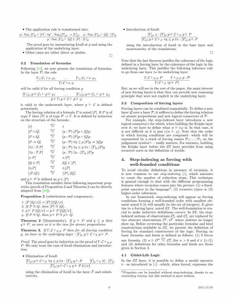
• The application rule is transformed into:
p : Nat, [Γ]p ⊢ [P ] : ∀p′ : Natp[T ]p′ → [U ]p′ p : Nat, [Γ]p ⊢ [Q] : [T ]p
p : Nat, [Γ]p ⊢ [Q] ∈ [P ] : [U ]p
The proof goes by instantiating forall at p and using theapplication of the underlying layer.
• Other cases are either direct or similar.
3.2 Translation of formulas
Following [16], we now present the translation of formulas.In the layer P, the rule
Γ1; C1 ⊢P ϕ1 . . . Γn; Cn ⊢P ϕn
Γ; C ⊢P ϕ
will be valid if for all forcing condition p
[Γ1]p; p C1 ⊢ p ϕ1 . . . [Γn]p; p Cn ⊢ p ϕn
p Γ; p C ⊢ p ϕ
is valid in the underneath layer, where p C is definedpointwisely.
The forcing relation of a formula P is noted [P ]. If P is oftype T then [P ] is of type P → T . It is defined by inductionon the structure of the formula :
[x]def= x
[P ∧Q]def= (p : P).[P ]p ∧ [Q]p
[P ∨Q]def= (p : P).[P ]p ∨ [Q]p
[P ⇒ Q]def= (p : P).∀q ≤ p.[P ]q ⇒ [Q]p
[∀x : T.P ]def= (p : P).∀q ≤ p.∀x : [T ]q.[P ]q
[∃x : T.P ]def= (p : P).∃x : [T ]q.[P ]p
[x.P ]def= x.[P ]
[Q ∈ P ]def= [Q] ∈ [P ]
[πiP ]def= πi[P ]
[〈P,Q〉]def= 〈[P ], [Q]〉
and p P is defined as p ∈ [P ].This translation satisfies these following important prop-
erties (proofs of Proposition 2 and Theorem 2 can be directlyadapted from [16]).
Proposition 2 (substitution and congruence).
1. [P Q/x] = [P ] [Q]/x.2. If P ∼= Q, then [P ] ∼= [Q].3. p P Q/x = p P [Q]/x.4. If P ∼= Q, then p P ∼= p Q.
Theorem 2 (Monotonicity). If p P and q ≤ p thenq P , as soon as it is the case for atomic propositions.
Theorem 3. If Γ, C ⊢P;F P then for all forcing conditionp, we have in the underlying layer : [Γ]p, p C ⊢F p P .
Proof. The proof goes by induction on the proof of Γ, C ⊢P;F
P . We only treat the case of forall elimination and introduc-tion.
• Elimination of forall:
[Γ]p; p C ⊢F ∀q ≤ p.∀x : [T ]q.q P [Γ]p ⊢F [t] : [T ]p
[Γ]p; p C ⊢F p P t/x
using the elimination of forall in the layer F and substi-tutivity.
• Introduction of forall:
[Γ]p, x : [T ]p; p C ⊢F p P
[Γ]p; p C ⊢F ∀q ≤ p.∀x : [T ]q.q P
using the introduction of forall in the base layer andmonotonicity of the translations.
Note that the last theorem justifies the coherence of the logicdefined in a forcing layer by the coherence of the logic in theunderlying layer. This justifies the following inference ruleto go from one layer to its underlying layer
Γ; C ⊢F;P P Γ ⊢F;P p : P
Γ; C ⊢F (p P )
But, as we will see in the rest of the paper, the main interestof new forcing layers is that they can provide new reasoningprinciple that were not explicit in the underlying layer.
3.3 Composition of forcing layers
Forcing layers can be combined sequentially. To define a newlayerQ over a layer P, it suffices to define the forcing relationon atomic propositions and new logical connectors of P.
For example, the step-indexed layer introduces a newlogical connector ⊲ for which, when building the Kripke layerover it, we have to define what w ⊲ϕ is. In that case, itis not difficult as it is just ⊲(w ϕ). Note that the orderin which forcing conditions are composed—which will berepresented by a stack of forcing names P1; . . . ;Pn on thejudgement symbol ⊢—really matters. For instance, buildingthe Kripke layer before the SI layer provides from usingrecursive sorts in the definition of worlds.
4. Step-indexing as forcing with
well-founded conditions
To avoid circular definitions in presence of recursion, itis now common to use step-indexing [3], which amountsto count the number of reduction steps. This techniqueis general enough to deal with the different programmingfeatures where recursion comes into the picture: (1) a fixed-point operator in the language2, (2) recursive types or (3)higher-order references.
In our framework, step-indexing will appear as forcingconditions forming a well-founded order with smallest ele-ment noted 0 (it will usually be the set of integers). It givesrise to a forcing layer, noted SI. The well-foundation is cru-cial to make inductive definitions correct. In SI, the step-indexed notions of observations Ol
n and Orn are replaced by
two abstract observations Ol, Or where indexes no longershow up. Before reviewing the particular formulas and kindconstructions available in SI, we present the definition offorcing for standard constructors of the logic. Forcing onbasic formulas and kinds is defined as follows: (1) 0 forces
any formula, (2) n Od def= Od
n (for n > 0 and d ∈ r, l)and (3) definitions for other formulas and kinds are thosegiven in Section 3.
4.1 Godel-Lob Logic
In the SI layer, it is possible to define a modal operator⊲—as introduced in [4]—which, when forced, expresses the
2Fixpoints can be handled without step-indexing, thanks to anunwinding lemma, but this method is more tedious.
6 2011/3/30

fact that a property has to be true in the (strict) future:
p ⊲Pdef= ∀q : Predp. q P
where Predp is the sort of predecessors of an integer p,defined as
Pred0 = ⊥ and Predp+1 = Natp.
This new connector satisfies two principles stating that theSI layer forms a Godel-Lob logic:
⊲-MonoΓ; C1, C2 ⊢SI P
Γ; ⊲C1, C2 ⊢SI ⊲PLob
Γ; C, ⊲P ⊢SI P
Γ; C ⊢SI P
Proof. We will just prove the validity of the Lob rule, theother one is direct. Using the elimination rule of the impli-cation before going down to the underneath layer , the rulebecomes:
[Γ]n;n C ⊢ ∀m ≤ n. (∀k : Predm. k ϕ) ⇒ m ϕ
[Γ]n;n C ⊢ n ϕ
We prove this inference rule by proving m ≤ n ⇒ m ϕby induction on m, the case m = 0 being direct as 0 ϕ isalways true.
Note that the well-foundation of step-indexes is central tobe able to make an induction on forcing conditions.
There are also the usual distributivity rules of ⊲ over thelogical connectives (the symbol l indicates that the rule canbe used in both directions):
l ⊲-⇒Γ; C ⊢SI ⊲(P ⇒ Q)
Γ; C ⊢SI ⊲P ⇒ ⊲Ql ⊲-∧
Γ; C ⊢SI ⊲(P ∧Q)
Γ; C ⊢SI ⊲P ∧ ⊲Q
l ⊲-∨Γ; C ⊢SI ⊲(P ∨Q)
Γ; C ⊢SI ⊲P ∨ ⊲Q
⊲-∃Γ; C ⊢SI ⊲(∃x : T.P )
Γ; C ⊢SI ∃x : T. ⊲ P⊲-∀
Γ; C ⊢SI ⊲(∀x : T.P )
Γ; C ⊢SI ∀x : T. ⊲ P
Proof. Let’s prove the rule ⊲-∀. Leaving the layer SI, wehave to prove that
[Γ]n;n C ⊢SI ∀k : Predn.∀i : Natk.∀x : [T ]i.i P (x)
[Γ]n;n C ⊢SI ∀k : Natn.x : [T ]k.∀i : Predk.i P (x)
So let k : Natn, x : [T ]k and i : Predk. By monotonicity weknow that x : [T ]i and instantiating the premise with k = i,we know that i P (x) (as xi < n).
Using this modality, it is possible to reason about recursionabstractly as shown in [4]. To be able to reason about logicalrelations, we exhibit derived inference rules on observation,valid in SI, such as the following rule
Γ; C ⊢ (M1, h1) → (M ′
1, h′
1) Γ; C ⊢SI ⊲Ol((M ′
1, h′
1), (M2, h2))
Γ; C ⊢SI Ol((M1, h1), (M2, h2))
4.2 Recursive relations
Step-indexed forcing conditions enables to define recursiverelations in SI as
n µr.R(M1,M2)def= ∀k : Predn. k R µr.R/r (M1,M2)
The forcing definition is well-defined thanks to the decreas-ing of the index. Such recursive relations satisfy the following
inference rules:
RRel-TypeΓ, r : Rel ⊢SI R : Rel
Γ ⊢SI µr.R : Rel
RRel-InfΓ; C ⊢SI ⊲R µr.R/r (M1,M2)
Γ; C ⊢SI µr.R(M1,M2)
Note that compared to other works, we do not require thatrecursive relations are contractive, i.e. have a ⊲ in front ofeach occurrence of r. But to prove the membership of twoterms in a recursive relation, we have to reason in the future,as the Rule RRel-Inf indicates.
As explained in the introduction, using a recursive rela-tion, logical relations can be extended to recursive types:
V Jµα.τKηdef= µr.
(
(v1, v2).∃u1, u2 : Val.v1 = rollu1
∧v2 = rollu2 ∧ ⊲V JτKη,α 7→r (u1, u2))
4.3 Recursive kinds
In a recent study of step-indexing in the topos of trees [6],Birkedal et al. have introduced the notion of a later operatoron presheaves, which indicates that we could define suchan operator3 T (together with recursive kinds µT.U) atthe level of kinds in the SI layer. Indeed, the followingtranslation of kinds under step-indexed forcing conditions
[ T ]0def= ⊤
[ T ]p+1def= [T ]p
[µT.U ]0def= ⊤
[µT.U ]p+1def= [U [µ.T/T ]]p
gives rise to a stratified construction of kinds. The subtypingrelation is defined as the identity on the new kinds. Fromthose definitions, one can deduce the validity of the followingtyping rules
lRec-KindΓ ⊢SI P : U µT.U/T
Γ ⊢SI P : µT.U
lSwitch- ⊲Γ ⊢SI P : Prop
Γ ⊢SI ⊲P : Prop
lCommut-Γ ⊢SI P : (T → U)
Γ ⊢SI P : T → U
Mono-Γ ⊢SI P : T
Γ ⊢SI P : T
together with rules that say that vanishes in front of theatomic kinds (but Prop of course).
Proof. • Rec-Kind : [ U µT.U/T]n = [µT.U ]n.• Switch- ⊲ : For non null integer p, we have toequiderive
[Γ]p ⊢ [P ] : Predp → Prop
[Γ]p ⊢ n.∀q : Predn.q P : Natp → Prop
which comes from
[Γ]p, n : Predp ⊢ p P : Prop
[Γ]p, n : Natp, q : Predn ⊢ q P : Prop .
3We borrow this notation from [6], to differentiate it from ⊲ whichis used on propositions.
7 2011/3/30

The case p = 0 is direct using the canonical typing rulesof ⊥ and ⊤.
• Commut- :Case p = 0:[ (T → U)]0 = ⊤ <: ⊤ → ⊤ = [ T → U ]0Case p+ 1:[ T → U ]p+1 <: [ T → U ]p = [T → U ]p−1
(induction hypothesis) and [ T → U ]p+1 <:[T ]p → [U ]p. So [ T → U ]p+1 <: [T → U ]p.The same holds for the other direction.
• Mono- : We use the fact that [T ]n <: [ T ]n.
Such recursive kinds will be used to build recursive worlds(Section 5.2), and will explain the presence of ⊲ in thedifferent definitions of logical relations involving recursiveworlds.
4.4 Equational reasoning
One of the main problem of step-indexing is that it is inher-ently asymmetric in the sense that going from inequationalto equational logical reasoning is not automatic. Indeed,from a step-indexed order logical relation 4
τn which links
two terms at level n, the induced equivalence M1 ≃τn M2
does not satisfy the following extensional property:
If ∀(u1, u2), u1 ≃τn u2 ⇒M1 u1 ≃σ
n M2 u2 then M1 ≃τ→σn M2
To avoid this problem, the idea—which first appears in[11]—is to use a parameter indicating what direction of theproof is to be proved.
To embody this parametric technique in our logic, weintroduce a new layer D, whose forcing conditions is the setl, r, flat-ordered by equality. In this layer, there is onlyone notion of observation, which is O. The forcing conditionis then defined by:
l Odef= Ol and r O
def= Or
and is transparent for the other formulas and kinds of SI.A reasoning in the SI;D layer has to be true for l and rindifferently, so it corresponds to an equational reasoning.Some derivable rules valid in the layer SI,D are shown inthe Figures 6 and 7.
5. Kripke Logical Relation
We now express another use of forcing conditions—the con-struction of worlds for Kripke logical relations. It is well-known that Kripke model can be seen as forcing, so thisshould not appear as a surprise. What is interesting here isthe interaction between the Kripke layer and other alreadydefined forcing layers.
Note that compared to step-indexing, it is not possibleto hide the reasoning on worlds, since there is a crucialinteraction between worlds and terms. So in this layer (whichwill be called the K layer), we do not really get new logicalprinciples as it was the case for the SI layer, but we ratherget a new symbol W in the logic which enables to talk aboutthe heap in formulas. Using this new symbol, the definitionof the logical relation at type ref τ is given by
V Jref τKη (l1, l2)def= ∀v1, v2 : τ. W(l1, l2)(v1, v2)
⇐⇒ (v1, v2) ∈ ⊲V JτKη
It says that two locations are related at type ref τ if thevalues v1, v2 related in the current world at those locationsare exactly the values that are related at type τ (in thefuture).
This means that to define Kripke logical relations over aset of worlds, we simply have to define
w W and w O
where O means any notion of observation. The rest of thedefinitions for formulas and kinds is straightforward. Forcingan observation with a world w is independent of the verynature of the observation, since w O((M1, h1), (M2, h2))ise defined as
(h1, h2) : w ⇒ O((M1, h1)(M2, h2)).
It is just a restriction of the observation to heaps related inthe world w, where the formula (h1, h2) : w in the definitionabove is a short-hand for
∀l1, l2 ∈ dom(w). w W(l1, l2)(h1(l1), h2(l2)).
This explains why the layer K can be defined above SI orD indifferently, where the new logical connectors introducedin SI are forced transparently as in the rule
w ⊲ϕdef= ⊲(w ϕ).
Those transparent definitions ensure that the new reasoningprinciples available in SI are still valid in the layer K.
As it is the case for Kripke models, an important factis that the set of worlds has to be ordered (usually notedw′ ⊒ w and pronounced w′ future of w) in order to providea good notion of forcing conditions. Note that we require thedefinition of forcing for the observation to be monotonous,which is the case in this paper but would not be the case forcomplex notion of worlds using STSs [12]. Nevertheless, it ispossible to relax monotony conditions by the use of modalforcing which makes explicit any need of monotonicity (seeSection 9).
5.1 First-order References
For first-order references, worlds (i.e. forcing conditions)have the kind
Worlddef= (Loc× Loc) →fin Rel
and the meaning of W is simply given by
w W(l1, l2)(v1, v2)def= w(l1, l2)(v1, v2)
This reconstructs logical relations defined by Pitts andStark [17]. Note that in that case, we make no use of thenew logical principles available in the SI layer.
5.2 Higher-order references in SI
Dealing with higher-order references requires to defineworlds recursively. This means that we must make use ofrecursive kinds available In the SI layer. For higher-orderreferences, worlds (i.e. forcing conditions) have the kind
Worlddef= µW.(Loc× Loc →fin W → Rel),
which corresponds to the one used in the semantics model4
of [7]. Using the typing rule of SI, one can see that the only“typable” definition of W is the following (used for instancein [12]):
w W(l1, l2)(v1, v2)def= ⊲w(l1, l2)(w)(v1, v2)
4 In [7] and previous works, the authors needs a monotonic func-tions space between W and Rel. It appears that—through forcingconstruction—any arrow in the K layer is monotonic so we haveit for free in our framework.
8 2011/3/30

Indeed, the typing derivation is
Ax
↑Rec-KindΓ ⊢ w : World
↓Commut-Γ ⊢ w : (Loc× Loc →fin World → Rel)
AppΓ ⊢ w : T Γ ⊢ l1, l2 : Loc · · ·
↓Switch ⊲Γ ⊢ w(l1, l2)(w)(v1, v2) : Prop
Γ ⊢ ⊲w(l1, l2)(w)(v1, v2) : Prop
where Γ and T are respectively
w : World, l1, l2 : Loc, v1, v2 : Term
and
Loc× Loc →fin World → (Term× Term) → Prop
5.3 Reasoning in the K layer
Let C′ = C, (h1, h2) : w and Ow = w O. Figure 6 presentsthe derived rules on Ow. As said before, those rules arenot expressible in the layer K as a precise knowledge of thecurrent world is required. Nevertheless, when the heap is notmodified by the reduction, we can reason directly in the layerK. Indeed, the previous inference rules can be written in thelayers ⊢K;SI and ⊢D;K;SI , forgetting any hypothesis aboutheaps hi. Hence, inference rules on E JτK can be deduced(see Figure 7, the proof of Step-D;K;SI-⊲E is given inAppendix).
Finally, due to the definition of forcing in D and K, wecan show that their forcing relations commute, which issometime useful when we want to exit one of the two layer.
6. Properties of Logical Relations
Now that logical relations are defined for the whole language,let us look at its soundness with respect to observationalequivalence. The proof of soundness for the pure fragmentcan be done in the SI;D;K layer as it can be completelyabstracted with respect to worlds. Indeed, pure terms doesnot change heap. Such a proof can then be instantiated byany world, going down to the SI;D layer. When dealing withthe impure fragment, we have to leave the K layer since weneed to know the world under consideration precisely. Andin the same way, when making an asymmetric reasoning,we will leave the layer D in order to work with a concretedirection (left or right).
6.1 Compatibility lemmas
To establish the correctness of our logical relation E JτK, wefirst prove the so-called compatibility lemmas of Figure 8.We just give the prove the compatibility for Fix, Roll andAssign. The rest of the proof can be found in appendix.
Proof. • Rule Fix :Using the rule V-to-E , we just have to prove thatΓ; C ⊢D,K,SI V Jτ → σK (fix f(x).M1, fix f(x).M2). To doso, we use the Lob rule, so we have to prove
Γ; C, ⊲(V Jτ → σK (fix f(x).M1, fix f(x).M2))︸ ︷︷ ︸
C′
⊢D,K,SI V Jτ → σK (fix f(x).M1, fix f(x).M2)
Unwinding the definition, we will prove that
Γ, v1 : τ, v2 : τ ; C′,V JτK (v1, v2)
⊢D,K,SI E Jτ → σK ((fix f(x).M1)v1, (fix f(x).M2)v2)
Using the rule Step-D;K;SI-⊲E , we just have to provethat
Γ′; C′ ⊢D,K,SI ⊲(E JσK (M1 v1/x f1/f ,M2 v2/x f1/f))
and using the rule ⊲-Mono we can conclude using thepremise.
• Rule Roll :Let K1,K2 two contexts s.t. K Jµα.τKη (K1,K2), we willprove that K Jτ µα.τ/αKη (K1[roll ],K2[roll ]).Let v1, v2 two values s.t. V Jτ µα.τ/αKη (v1, v2), thenwe have to prove that
∀h1, h2.O((K1[roll v1], h1), (K2[roll v2], h2))
which is direct since, by monotony and substitution wehave
⊲(V JτKη,α 7→VJµα.τKη
(v1, v2))
so
V Jµα.τKη (roll v1, roll v2).
• Rule Assign :Let K1,K2 two contexts s.t. K JUnitKη (K1,K2), we willprove that K Jref τKη (K1[ := M1],K2[ := M2]). So letl1, l2 two values s.t. V Jref τKη (l1, l2) we have to prove
∀h1, h2.O((K1[l1 :=M1], h1), (K2[l2 :=M2], h2))
To do so, we will prove that K JτKη (K1[l1 := ],K2[l2 :=]). Let v1, v2 two values s.t. V JτKη (v1, v2) we have toprove
∀h1, h2.O((K1[l1 := v1], h1), (K2[l2 := v2], h2))
Leaving the layer K, suppose h1, h2 : w then from w
V Jref τKη (l1, l2) we get that li ∈ dom(hi).Then we conclude, using the rules StepL-K;SI-E andStepR-K;SI-E , by showing that
w O((K1[()], h1[l1 7→ v1]), (K2[()], h2[l2 7→ v2]))
using the fact that w K JUnitKη (K1,K2) and (h1[l1 7→v1), h2[l2 7→ v2]) : w.
An other crucial derived rule is the adequacy between V JτKand E JτK over values :
V-to-EΓ; C ⊢D,K,SI V JτK (M1,M2)
Γ; C ⊢D,K,SI E JτK (M1,M2)
6.2 Soundness of logical relations
Now we prove the soundness of our logical relation withrespect to the contextual equivalence, following the usualschema of [13].
Theorem 4. Fundamental property If ∆;Υ; Γ ⊢ t : τ then
⊢D,K,SI t ≃∆;Υ;Γ
log t : τ .
By induction on the typing rule, in each case using theprevious compatibility lemmas.
Theorem 5. Congruence If ⊢ M1 ≃∆;Υ;Γ
log M2 : τ and
⊢ C : (∆;Υ; Γ ⊢ τ) → (∆′; Υ′; Γ′ ⊢ σ) then ∆;Υ; Γ ⊢C[M1] ≃log C[M2] : τ .
The proof is done by induction on the context C, usingagain compatibility lemmas.
Theorem 6. Adequacy If M1 ≃·,·,Υlog M2 : τ then for all heap
h satisfying Υ, O((M1, h), (M2, h)).
9 2011/3/30

Step-Olw
Γ; C′ ⊢ (M1, h1) → (M ′1, h
′1) Γ; C′ ⊢SI (h′
1, h2) : w′ Γ; C′ ⊢SI Ol
w′ ((M′1, h
′1), (M2, h2))
Γ; C ⊢SI Olw((M1, h1), (M2, h2))
and the dual rule for r
Step-⊲Olw
Γ; C′ ⊢ (M1, h1) → (M ′1, h
′1) Γ; C′ ⊢SI (h′
1, h2) : w′ Γ; C′ ⊢SI ⊲Ol
w′ ((M′1, h
′1), (M2, h2))
Γ; C ⊢SI Olw((M1, h1), (M2, h2))
and the dual rule for r
Step-⊲Ow
Γ; C′ ⊢ (Mi, hi) → (M ′i , h
′i) i ∈ 1, 2 Γ; C′ ⊢D;SI (h′
1, h′2) : w
′ Γ; C′ ⊢D;SI ⊲Ow′ ((M ′1, h
′1), (M
′2, h
′2))
Γ; C ⊢D;SI Ow((M1, h1), (M2, h2))
Figure 6. Derived rules on Ow
StepL-K;SI-EΓ; C ⊢ (M1, h1) → (M ′
1, h1) Γ; C ⊢K;SI l E JτK ((M ′
1, h1), (M2, h2))
Γ; C ⊢K;SI l E JτK ((M1, h1), (M2, h2))and the dual rule for r
StepL-K;SI-⊲EΓ; C ⊢ (M1, h1) → (M ′
1, h′
1) Γ; C ⊢K;SI l ⊲E JτK ((M ′
1, h′
1), (M2, h2))
Γ; C ⊢K;SI l E JτK ((M1, h1), (M2, h2))and the dual rule for r
Step-D;K;SI-⊲EΓ; C ⊢ (Mi, hi) → (M ′
i , hi) (i = 1, 2) Γ; C ⊢D;K;SI ⊲E JτK (M ′
1,M′
2)
Γ; C ⊢D;K;SI E JτK (M1,M2)
Figure 7. Derived rules on E JτK for the layer K;SI
To prove it, we just have to show that the empty contextis in K JτK.
Theorem 7. Soundness If ⊢D,K,SI M1 ≃∆;Υ;Γ
log M2 : τ then
⊢D,K,SI M1 ≃∆;Υ;Γctx M2 : τ .
Direct by combining adequacy and congruence lemmas.
7. An example : the Landin Knot
To illustrate our work, we are going to show that the well-known Landin knot is logically equivalent to the usual fix-point operator. Following [13], we consider
M1 = let y = ref (λx.⊥) in y:= (λ x.let f = !y ine);!y
and
M2 = fix λ f(x).e
and we will prove that ⊢D,K,SI (M1,M2) ∈ E Jτ → σK.Unwinding the definition of E Jτ → σK, we have to prove that
(K1,K2) ∈ K Jτ → σK ⊢D,K,SI
((K1[M1], h1), (K2[M2], h2)) ∈ O
Leaving the layer K, we have to prove that those two termsare in Ow for every world w. Then, we use the rule Step-Ol
w
with the fact that (K1[M1], h1) reduce to
(λx.let f = !l in e︸ ︷︷ ︸
M′
1
, h1 • [l 7→ λx.let f = !l in e]︸ ︷︷ ︸
h′
1
)
So we build a world w′ ⊒ w which restrains l to always pointin h1 to λx.let f = !l in e :
w′ = w • [(l, l) 7→ R]
where R is the relation (t1, t2).t1 = λx.let f = !l in e.So we just have to prove that w′
(M ′1,M2) ∈ E Jτ → σK.
To do so, we use the rule V-to-E and the Lob rule, and thus
prove that
⊲(w′ (M ′
1,M2) ∈ V Jτ → σK︸ ︷︷ ︸
C1
) ⊢D;SI
w′ (M ′
1,M2) ∈ V Jτ → σK
Using the rule Abstr in the layer D;SI, then the rule Step-D;K;SI-⊲E , this amount to prove
Γ; ⊲C1; C2 ⊢D;SI
w′ ⊲(e v1/x M
′1/f , e v2/x M2/f) ∈ E JσK
where Γ is l : Loc, v1, v2 : τ and C2 is (v1, v2) ∈ V JτK. Then,using the rule Mono-⊲, we make the ⊲ disappear and weconclude using the rule App with the hypothesis C1, C2.
8. Related works
8.1 Syntactic models
The difficulties encountered to build logical relations forFµ! also appear at the semantic model level. Indeed, thosemodels—associating to each type a set of terms—can some-how be seen as unary version of logical relations.
The very modal model [4] introduces the stratification ofworlds and the ⊲ operator, following the idea that derefer-encing will always take at least one step of reduction. In thisway properties about the value stocked there only have tobe proved in the strict future.
In [19], F. Pottier gives a typed store-passing transla-tion for higher-order references. This syntactic constructionis based on Nakano’s system, introducing co-inductively de-fined kinds with well-formation defined thanks to a “later”modality on those kinds. As it is the case for [7], there areclear connections between this syntactic presentation andthe logical principles available in the SI layer.
8.2 Topos of trees
In [6], Birkedal et al. define a semantic model of a languagesimilar to Fµ!, built over the topos of trees (i.e. of presheavesover ω). It appears that this topos constitutes a model of
10 2011/3/30

Abstr
Γ, v1 : τ, v2 : τ ; C,V JτKη (v1, v2) ⊢D,K,SI E JσKη (M1 v1/x ,M2 v2/x)
Γ; C ⊢D,K,SI E Jτ → σKη (λx.M1, λx.M2)
App
Γ; C ⊢D,K,SI E Jτ → σKη (M1,M2) Γ; C ⊢D,K,SI E JτKη (N1, N2)
Γ; C ⊢D,K,SI E JσKη (M1N1,M2N2)
FixΓ, v1 : τ, v2 : τ ; C,V JτKη (v1, v2),V Jτ → σKη (f2, f1) ⊢D,K,SI E JσKη (M1 v1/x f1/f ,M2 v2/x f1/f)
Γ; C ⊢D,K,SI E Jτ → σKη (fix f(x).M1︸ ︷︷ ︸
f1
, fix f(x).M2)︸ ︷︷ ︸
f2
Gen
Γ, α1 : Type, α2 : Type, r : Relα1,α2; C ⊢D,K,SI E JτKη,α 7→r (M1 α1/α ,M2 α1/α)
Γ; C ⊢D,K,SI E J∀α.τKη (Λα.M1,Λα.M2)
Inst
Γ; C ⊢D,K,SI E J∀α.τKη (M1,M2) Γ ⊢D,K,SI σ : Type
Γ; C ⊢D,K,SI E Jτ σ/τKη (M1σ,M2σ)
Roll
Γ; C ⊢D,K,SI E Jτ µα.τ/αKη (M1,M2)
Γ; C ⊢D,K,SI E Jµα.τKη (rollM1, rollM2)Unroll
Γ; C ⊢D,K,SI E Jµα.τKη (M1,M2)
Γ; C ⊢D,K,SI E Jτ µα.τ/αKη (unrollM1, unrollM2)
Alloc
Γ; C ⊢D,K,SI E JτKη (M1,M2)
Γ; C ⊢D,K,SI E Jref τKη (refM1, refM2)Deref
Γ; C ⊢D,K,SI E Jref τKη (M1,M2)
Γ; C ⊢D,K,SI E JτKη (!M1, !M2)
Assign
Γ; C ⊢D,K,SI E Jref τKη (M1,M2) Γ; C ⊢D,K,SI E JτKη (N1, N2)
Γ; C ⊢D,K,SI E JτKη (M1 := N1,M2 := N2)
Figure 8. Compatibility lemmas
our SI layer—even so we don’t need models to testimonythe consistency of our logic as we just translate it intoFLR using forcing definitions. This should not appear as asurprise as Cohen forcing can be rephrased in topos theory,following the work of Lawvere and Thierney [20].
More precisely, a predicate ϕ in the layer SI is seen as anω-valued function, mapping to the set of indexes which forceit. The stratification of sorts appearing in the SI layer corre-sponds to the construction of presheaves. The stratificationof Prop induced by forcing conditions corresponds exactly tothe definition of the subobject classifier Ω of the topos. Thefact that the translation of sorts is constant but for Prop andµT.U follows from the idea that constant presheaves (i.e. thelogic of the tripos over ω) are enough to model LSLR.
8.3 LSLR and LADR
LSLR [11] is an extension of Abadi-Plotkin logic to reasonabout equivalence of λ-terms with polymorphism and re-cursive types. LADR [13] is an extension of LSLR to proveequivalence of λ-terms with higher-order states, e.g. usingKripke logical relations. Both logics make step-indexing ab-stract using Godel-Lob logic and a ⊲ operator. But to buildrecursive worlds in LADR, the authors use an explicit strat-ification which makes step-indexes apparent. It should bepossible to integrate their construction in our system, justlike the refinement of [12], without making any step-indexvisible in the layer SI, using recursive kinds.
Our approach is really different from LSLR and LADR:we do not rely on any particular model to prove the co-herence of our logic. Indeed, the coherence of the differentforcing layers comes directly from the translation of propo-sitions in the core logic.
Definitions of recursive relations µr.R in LSLR must sat-isfy a syntactic criterion of contractivity, which enforces thepresence of ⊲ in front of each occurrence of the variable r.This criterion is crucial to build their model. Our approachis different since the ⊲ operator is not in the definition of re-cursive relations but appears through a particular inferencerule that unfolds the definition of µr.R only in the future.
Compared to LSLR, we do not count only roll and unrollreductions in step-indexes, but decides that every reductionmatters. Then, using the rule ⊲-Mono, it is possible to eraseoccurrences of ⊲ that will not be relevant in the proof. Doingso, step-indexing can be used to deal with fixpoint operator,but it is no longer guided by the inference rules, as it is thecase with the ⊳ in LSLR.
Finally, the idea of a direction parameter d to deal withthe problem of equational reasoning in presence of step-indexing appeared first in LSLR, where it is simply a termvariable of type bool, which always appear in the typingcontext Γ. This idea is then refined in LADR where theparameter appears in the definition of worlds. Here, we goone step further and define a proper forcing layer D wherewe can deal with equational reasoning.
9. Future work
Monotonicity and modal forcing What we have pre-sented here correspond to intuitionnistic forcing, since themonotonicity is imposed by the definition of p P ⇒ Qand p ∀x : T.P . This is enough to deal with worlds seenas invariants on heap. But recent works in [2] and [12] havedeveloped notions of worlds which described the evolutionof the heap. To deal with such works in our framework, we
11 2011/3/30

would need to relax the monotonicity of our forcing relation,and rather add a modality just as in [13]
p Pdef= ∀q ≤ p.q P.
Using this modality, we can explicitly state were monotonic-ity has to be enforced and where it is not relevant. In thesame way we could deal with public and private transitionof [12] by splitting the order of forcing condition into twoparts.
Finer description of the heap It would be interesting tosee if relational separation logic can be used to link abstractworlds and heaps, as in [12]. Then, temporal logic could beused to reason about STSs, which are used to restrict thepossible futures of worlds. The problem with this methodis that the order on worlds is eminently not linear, so wehave to keep track of each choice made while moving in thefuture. This is done in LADR using island contexts. Withsuch an extension of our framework we would be able toexpress useful derived rules for programs modifying theirheap, without leaving the layer K.
Implicit Complexity A recent work of Hofmann and DalLago on a realizability model for implicit complexity typesystem [10] uses a notion of resource monoid which fitswell in our framework, when working with a predicative(as opposed to relational) notion of termination for theobservation. This would be an example where the order onforcing conditions in the SI layer is not linear.
Subset types Some of the properties of our logic, like thekinds Natp and T →fin U , could be defined using usualsubset types. However, adding them in our framework is noteasy, since we would then have to define the forcing transla-tion of such sorts. This seems anyway possible following thetranslation of proofs induced by forcing given in [16].
Formalization in Coq Formalizing this work in Coqwould not be totally easy due to the lack of implicit de-pendent types in CIC. So this requires a deep embedding ofthe logic. An other possibility would be to avoid the use ofimplicit depend types by constraining the monotonicity of[T → U ] directly in the definition (using record types).
10. Conclusion
In this paper, we decompose the construction of logical re-lations for a language with recursive types and higher-orderreferences. This is achieved by reunderstanding Cohen’s forc-ing as a way to increase step-by-step the power of a logicalsetting. The first step is to extend the logic with the Lobrule, recursive relations and recursive kinds by means of forc-ing with step indexes which stratify formulas and kinds. Thesecond step is to encompass the asymmetric nature of proofsof equivalence by means of forcing with two elements repre-senting the left and right orientation. Finally, the last step isto extend the model with a notion of recursive worlds (basedon recursive kinds provided by step-indexes), which—whenseeing as forcing conditions—defines directly the usual no-tion of Kripke logical relations. One of the main achievementof this paper is to build complex notion of worlds directlyinside the logic. We believe that the use of forcing conditionsopens the door to the definition of richer logical relations todeal with concurrent or design specific languages.
Acknowledgments
The authors want to thank Lars Birkedal and AlexandreMiquel for valuable discussions.
References
[1] A. Ahmed. Step-indexed syntactic logical relations for re-cursive and quantified types. Programming Languages andSystems, pages 69–83, 2006.
[2] A.W. Ahmed, D. Dreyer, and A. Rossberg. State-dependentrepresentation independence. In Proceedings of the 36thACM Symposium on Principles of Programming Languages,2009.
[3] A.W. Appel and D. McAllester. An indexed modelof recursive types for foundational proof-carrying code.ACM Transactions on Programming Languages and Systems(TOPLAS), 23(5):657–683, 2001.
[4] A.W. Appel, P.-A. Mellies, C.D. Richards, and J. Vouillon. Avery modal model of a modern, major, general type system.In Proceedings of the 34th ACM Symposium on Principlesof Programming Languages, 2007.
[5] J. Avigad. Forcing in proof theory. The Bulletin of SymbolicLogic, 10(3):305–333, 2004.
[6] L. Birkedal, R. Møgelberg, J. Schwinghammer, andK. Støvring. First steps in synthetic guarded domain theory:step-indexing in the topos of trees. In Logic in ComputerScience (to appear), 2011.
[7] L. Birkedal, B. Reus, J. Schwinghammer, K. Støvring,J. Thamsborg, and H. Yang. Step-indexed Kripke modelsover recursive worlds. In Proceedings of the 38th ACM Sym-posium on Principles of Programming Languages, 2011.
[8] P.J. Cohen and M. Davis. Set theory and the continuumhypothesis. WA Benjamin New York, 1966.
[9] T. Coquand and G. Jaber. A Note on Forcing and TypeTheory. Fundamenta Informaticae, 100(1):43–52, 2010.
[10] Ugo Dal Lago and Martin Hofmann. A semantic proof ofpolytime soundness for light affine logic. Theory of Comput-ing Systems, 2009. to appear.
[11] D. Dreyer, A. Ahmed, and L. Birkedal. Logical step-indexedlogical relations. In Proceedings of the 24th Annual IEEESymposium on Logic In Computer Science, 2009.
[12] D. Dreyer, G. Neis, and L. Birkedal. The impact of higher-order state and control effects on local relational reasoning.In Proceedings of the 15th ACM International Conferenceon Functional programming, 2010.
[13] D. Dreyer, G. Neis, A. Rossberg, and L. Birkedal. A relationalmodal logic for higher-order stateful ADTs. In Proceedingsof the 38th ACM Symposium on Principles of ProgrammingLanguages, 2010.
[14] Jean-Louis Krivine. Structures de realisabilite, RAM etultrafiltre sur N.
[15] A. Miquel. A model for impredicative type systems, uni-verses, intersection types and subtyping. In Logic in Com-puter Science, pages 18–29. IEEE, 2002.
[16] A. Miquel. Forcing as a program transformation. In Logic inComputer Science (to appear), 2011.
[17] A. M. Pitts and I. D. B. Stark. Operational reasoning forfunctions with local state. In Higher Order OperationalTechniques in Semantics. CUP, 1998.
[18] G. Plotkin and M. Abadi. A logic for parametric polymor-phism. In Typed Lambda Calculi and Applications, 1993.
[19] F. Pottier. A typed store-passing translation for generalreferences. In Proceedings of the 38th ACM Symposium onPrinciples of Programming Languages, 2011.
[20] M. Tierney. Sheaf theory and the continuum hypothesis.LNM 274, pages 13–42, 1972.
12 2011/3/30

Appendix
Typing rules for partial finite functions.
(x : τ) ∈ Γ
∆;Υ; Γ ⊢ x : τ ∆;Υ; Γ ⊢ () : Unit ∆;Υ; Γ ⊢ n : Nat
∆;Υ; Γ ⊢M : τ → σ ∆;Υ; Γ ⊢ N : τ
∆;Υ; Γ ⊢MN : σ
∆;Υ; Γ, x : τ ⊢M : σ
∆;Υ; Γ ⊢ λx.M : τ → σ
∆;Υ; Γ, x : τ, f : τ → σ ⊢M : σ
∆;Υ; Γ ⊢ fix f(x).M : τ → σ
∆;Υ; Γ ⊢M : ∀α.τ FV (σ) ⊆ ∆
∆;Υ; Γ ⊢Mσ : τ σ/α
∆, α; Υ; Γ ⊢M : τ
∆;Υ; Γ ⊢ Λα.M : ∀α.τ
∆;Υ; Γ ⊢M : µα.τ
∆;Υ; Γ ⊢ unrollM : τ µα.τ/α
∆, α; Υ; Γ ⊢M : τ µα.τ/α FV (τ) ⊆ ∆ ∪ α
∆;Υ; Γ ⊢ rollM : µα.τ
∆;Υ; Γ ⊢ l : ref Υ(l)
∆;Υ; Γ ⊢ M : ref τ
∆;Υ; Γ ⊢!M : τ
∆;Υ; Γ ⊢ M : ref τ ∆;Υ; Γ ⊢ N : τ
∆;Υ; Γ ⊢ M := N : Unit
Typing rules for partial finite functions.
Γ ⊢ f : A→fin B
Γ ⊢ dom(f) : A→ Prop
Γ ⊢ f : A→fin B
Γ ⊢ f : A→ B Γ ⊢ emp : A→fin B
Γ ⊢ f : A→fin B Γ ⊢ u : A Γ ⊢ v : B
Γ ⊢ f • [u 7→ v] : A→fin B
Γ ⊢ f : A→fin B Γ ⊢ u : A Γ ⊢ v : B
Γ ⊢ f [u 7→ v] : A→fin B
Compatibily lemmas.
• Rule Abstr :
Using the rule V-to-E , we just have to prove that Γ; C ⊢D,K,SI V Jτ → σK (λx.M1, λx.M2). Unwinding the definition, wewill prove that
Γ, v1 : τ, v2 : τ ; C,V JτK (v1, v2) ⊢D,K,SI E Jτ → σK ((λx.M1)v1, (λx.M2)v2)
and we conclude using the rule StepS-E .
• Rule App :
LetK1,K2 s.t.K JσK (K1,K2), we will prove thatK Jτ → σK (K1[N1],K2[N2]). So letM′1,M
′2 s.t. V Jτ → σK (λx.M ′
1, λx.M′2),
then we must show
∀h1, h2.O((K1[(λx.M′
1)N1], h1),K2[(λx.M′
2)N2], h2)
Using the fact that E JτK (N1, N2), we just have to prove that K JτK (K1[(λx.M′1)],K2[(λx.M
′2)]). so taking v1, v2 s.t.
V JτK (v1, v2) and we can conclude showing
∀h1, h2.O((K1[(λx.M′
1)v1], h1),K2[(λx.M′
2)v2], h2)
which comes from the fact that E JσK ((λx.M ′1)v1, (λx.M
′2)v2) and K JσK (K1,K2).
• Rule Fix :
Using the rule V-to-E , we just have to prove that Γ; C ⊢D,K,SI V Jτ → σK (fix f(x).M1, fix f(x).M2). To do so, we use theLob rule, so we have to prove
Γ; C, ⊲(V Jτ → σK (fix f(x).M1, fix f(x).M2))︸ ︷︷ ︸
C′
⊢D,K,SI V Jτ → σK (fix f(x).M1, fix f(x).M2)
Unwinding the definition, we will prove that
Γ, v1 : τ, v2 : τ ; C′,V JτK (v1, v2) ⊢D,K,SI E Jτ → σK ((fix f(x).M1)v1, (fix f(x).M2)v2)
13 2011/3/30

Using the rule Step-D;K;SI-⊲E , we just have to prove that
Γ′; C′ ⊢D,K,SI ⊲(E JσK (M1 v1/x f1/f ,M2 v2/x f1/f))
and using the rule ⊲-Mono we can conclude using the premiss.
• Rule Gen :
Using the rule V-to-E , we just have to prove Γ; C ⊢D,K,SI V J∀α.τKη (Λα.M1,Λα.M2). So let α1, α2 two types andr : Relα1,α2
and we prove that
Γ, α1 : Type, α2 : Type, r : Relα1,α2; C ⊢D,K,SI E JτKη,α 7→r (((Λα.M1)α1, (Λα.M2)α2)
using the rule Step-D;K;SI-⊲E .
• Rule Inst :
Let K1,K2 two contexts s.t. K Jτ σ/αK (K1,K2), we will prove that
K J∀α.τK (K1[σ],K2[σ])
Indeed, let v1, v2 two values s.t. V J∀α.τK (v1, v2), we must show :
∀h1, h2.O((K1[v1σ], h1), (K2[v2σ], h2))
To do so, we use the fact that E JτKη,α 7→r (v1σ, v2σ) for all r : Relσ, that K Jτ σ/αKη (K1,K2) and the equality betweenE JτKη,α 7→VJσK
η
and E Jτ τ/αKη.
• Rule Unroll :
Let K1,K2 s.t. K Jτ µα.τ/αK (K1,K2), we just have to prove that K Jµα.τK (K1[unroll ],K2[unroll ]). So let v1, v2 s.t.V Jµα.τK (roll v1, roll v2), we will show that∀(h1, h2),O((K1[unroll roll v1], h1), (K2[unroll roll v2], h2)).
To do so, we know that ⊲E Jτ µα.τ/αK (v1, v2), i.e. ⊲O((K1[v1], h1), (K2[v2], h2)).
Then we conclude using the rule StepS-⊲O with the fact that (K[unroll roll vi], hi) → (K[vi], hi) with i ∈ 1, 2.
• Rule Roll :
Let K1,K2 two contexts s.t. K Jµα.τKη (K1,K2), we will prove that K Jτ µα.τ/αKη (K1[roll ],K2[roll ]).
Let v1, v2 two values s.t. V Jτ µα.τ/αKη (v1, v2), then we have to prove that
∀h1, h2.O((K1[roll v1], h1), (K2[roll v2], h2))
which is direct since, by monotony and substitution we have ⊲(V JτKη,α 7→VJµα.τKη
(v1, v2)) so V Jµα.τKη (roll v1, roll v2).
• Rule Alloc :
The proof takes place out of the layer K, so let w a world, we have to prove
Γ; C ⊢D;SI ∀w′ ⊒ w.w′ K JτKη (K
′
1,K′
2) ⇒ ∀(h1, h2).Ow′((K′
1[M1], h1), (K′
2[M2], h2))
Γ; C ⊢D;SI ∀w′ ⊒ w.w′ K Jref τKη (K1,K2) ⇒ ∀(h1, h2).Ow′((K1[refM1], h1), (K2[refM2], h2))
So let K1,K2 two contexts s.t. w′ K Jref τKη (K1,K2). We will prove that w′
K JτKη (K1[ref ],K2[ref ]). Taking
w′′ ⊒ w′ and v1, v2 two values s.t. w′′ V JτKη (v1, v2), we have to prove :
∀h1, h2.Ow′′((K1[ref v1], h1), (K2[ref v2], h2))
Let h1, h2 two heaps then (Ki[ref vi], hi) → (Ki[li], hi • [li 7→ vi]) with li /∈ dom(hi).
If (h1, h2) : w′′ then (l1, l2) /∈ dom(w′′), and we can build a new world
w0 = w′′ • [(l1, l2) 7→ (w).w V JτKη]
and using the rules StepL-K;SI-E and StepR-K;SI-E we just have to prove that
Ow0((K1[l1], h1 • [l1 7→ v1]), (K2[l2], h2 • [l2 7→ v2]))
which comes from the fact that (h1 • [l1 7→ v1], h2 • [l2 7→ v2]) : w0 and that w0 V Jref τKη (l1, l2), true by definition of w0.
14 2011/3/30

• Rule Deref :
The proof takes place out of the layer K, so let w a world, we have to prove
Γ; C ⊢D;SI ∀w′ ⊒ w.w′ K Jref τKη (K
′
1,K′
2) ⇒ ∀(h1, h2).Ow′((K′
1[M1], h1), (K′
2[M2], h2))
Γ; C ⊢D;SI ∀w′ ⊒ w.w′ K JτKη (K1,K2) ⇒ ∀(h1, h2).Ow′((K1[!M1], h1), (K2[!M2], h2))
LetK1,K2 two contexts s.t. w′ K JτKη (K1,K2), we will prove that w
′ K Jref τKη (K1[!],K2[!]). So let a world w′′ ⊒ w′
and two values l1, l2 s.t. w′′ V Jref τKη (l1, l2), we have to prove :
w′′ ∀h1, h2.O((K1[!l1], h1), (K2[!l2], h2))
Suppose h1, h2 : w′′ then using the fact that w′′ V Jref τKη (l1, l2), we know that (l1, l2) ∈ dom(w′′) because W(l1, l2) has
to be defined since V JτKη is not the empty relation. Then we can deduce that li ∈ dom(hi).
So using the rule Step-D;K;SI-⊲E with the same world, we just have to prove that
w′′ ⊲O((K1[h1(l1)], h1), (K2[h2(l2)], h2))
which come from the fact that w′′ ⊲V JτKη (h(l1), h(l2)). Indeed, h1, h2 : w′′ means w′′
W(l1, l2)(h1(l1), h2(l2)) and weconclude using the definition of V Jref τK.
• Rule Assign :
Let K1,K2 two contexts s.t. K JUnitKη (K1,K2), we will prove that K Jref τKη (K1[ :=M1],K2[ :=M2]). So let l1, l2 twovalues s.t. V Jref τKη (l1, l2) we have to prove :
∀h1, h2.O((K1[l1 :=M1], h1), (K2[l2 :=M2], h2))
To do so, we will prove that K JτKη (K1[l1 := ],K2[l2 := ]). Let v1, v2 two values s.t. V JτKη (v1, v2) we have to prove :
∀h1, h2.O((K1[l1 := v1], h1), (K2[l2 := v2], h2))
Leaving the layer K, suppose h1, h2 : w then from w V Jref τKη (l1, l2) we get that li ∈ dom(hi)
Then we conclude, using the rules StepL-K;SI-E and StepR-K;SI-E , by showing that :
w O((K1[()], h1[l1 7→ v1]), (K2[()], h2[l2 7→ v2]))
using the fact that w K JUnitKη (K1,K2) and (h1[l1 7→ v1), h2[l2 7→ v2]) : w
Proof tree for rule Step-D;K;SI-⊲E.
Γ′; C′ ⊢F (Mi, hi) → (M ′i , hi)
Γ′; C′ ⊢F (K1[Mi], hi) → (K2[M′i ], hi)
Γ′; C′ ⊢F K JτKη (K1,K2)
Γ′; C′ ⊢F ⊲K JτKη (K1,K2)
Γ′; C′ ⊢F ⊲E JτK (M ′1,M
′2)
Γ′; C′ ⊢F ⊲K JτKη (K1,K2) ⇒ ⊲O((K1[M1], h1), (K2[M2], h2))
Γ′; C′ ⊢F ⊲O((K1[M1], h1), (K2[M2], h2))
Γ,K1,K2 : Cont, h1, h2 : Heap; C,K JτKη (K1,K2) ⊢F O((K1[M1], h1), (K2[M2], h2))
Γ; C ⊢F ∀(K1,K2),K JτKη (K1,K2) ⇒ ∀h1, h2.O((K1[M1], h1), (K2[M2], h2))
where F = D;K;SI and Γ′; C′ = Γ,K1,K2 : Cont, h1, h2 : Heap; C,K JτKη (K1,K2).
15 2011/3/30