Embed Size (px)
Citation preview


DECLARATION
Stud.techn. Pia Glæserud
Institute of Industrial Economics and Technology Management
I hereby declare that I have written the above mentioned thesis without any kind of illegal assistance
___________________________ _________________________ Place Date
_____________________________________________ Signature
In accordance with Examination regulations § 20, this thesis, together with its figures etc., remains the property of the Norwegian University of Science and Technology (NTNU). Its contents, or results of them, may not be used for other purpose without the consent of the interested parties.


DECLARATION
Stud.techn. Jannicke Aschjem Syrdalen
Institute of Industrial Economics and Technology Management
I hereby declare that I have written the above mentioned thesis without any kind of illegal assistance
___________________________ _________________________ Place Date
_____________________________________________ Signature
In accordance with Examination regulations § 20, this thesis, together with its figures etc., remains the property of the Norwegian University of Science and Technology (NTNU). Its contents, or results of them, may not be used for other purpose without the consent of the interested parties.


Master Thesis
Optimization of Petroleum Production under
Uncertainty
-
Applied to the Troll C Field
Pia Glæserud and Jannicke Aschjem Syrdalen
Norwegian University of Science and Technology
Faculty of Social Sciences and Technology Management
Department of Industrial Economics and Technology Management
June 10, 2009


Preface
This Master thesis is the result of the �nal work accomplished to achieve a Masterof Science degree with specialization in Applied Economics and Optimization at theDepartment of Industrial Economics and Technology Management at the NorwegianUniversity of Science and Technology (NTNU).
The motivation for the thesis is the work by Gunnerud and Langvik (2007) and VestbøandWalberg (2008), presenting petroleum production optimization models for the Troll C�eld, initiated by the IO Center at NTNU and StatoilHydro. There has been a growinginterest in evaluating the e�ects of uncertainties related to the petroleum productionproblem, resulting in this thesis treating optimization under uncertainty applied to theTroll C �eld.
We have enjoyed working with the thesis, and acquiring knowledge about the petroleumindustry and optimization under uncertainty. A wide variety of theory on stochasticoptimization has been studied, which at times has been challenging, but also very inter-esting.
We would like to thank our supervisor, associate professor Asgeir Tomasgard, for con-structive discussions and guidance. Professor Bjarne Anton Foss at the Department ofEngineering Cybernetics has provided valuable input to the thesis. We are particularlygrateful for the time PhD candidate Vidar Gunnerud has devoted to us, giving insightto the problem and answering all types of questions. Additionally, we appreciate theinformation provided by former employee at StatoilHydro, Dr.Eng. Marta Dueñas Díez,and her belief in the project. We also thank PhD candidate Peter Schütz for his con-tributions on stochastic programming, and Dr. Andrew R. Conn at IBM T.J. WatsonResearch Center for his counseling on nonlinear solution methods.
Trondheim, June 10, 2009
Pia Glæserud Jannicke Aschjem Syrdalen
i


Abstract
The petroleum industry is a complex and capital-intensive sector, which implies a needfor extensive planning in order to obtain e�cient development and production. In thisthesis, optimization of the operational production planning problem at the Troll C �eld isconsidered. The operations are exposed to various risks and uncertainties, which shouldbe incorporated when developing productions plans.
Modeling the production system at Troll C is a challenging task, where �ow predictionsare essential. Due to the thin oil layer in the reservoir, estimating the wellstreams is dif-�cult, and the actual �ow may deviate from the predicted values. Moreover, the capacitylimit at the platform is varying, depending on external factors. If these uncertainties arenot accounted for in an optimization model, the capacity limit may be exceeded as aresult of the deviating model parameters.
Various methods of incorporating uncertainty in stochastic optimization models are pro-posed. The uncertainties at Troll C are treated at di�erent levels of the productionsystem, and both chance constrained and recourse models are presented for the planningproblem. These stochastic models are based on the deterministic formulation developedin the master thesis by Gunnerud and Langvik (2007).
The chance constrained model gives rise to a mixed integer nonlinear problem, whichis implemented in GAMS/BARON, whereas the recourse models are large scale mixedinteger linear problems solved in XpressMP. The results obtained indicate similar e�ectsof uncertainty in all the models. In general, higher uncertainty levels reduce the objectivevalue, and shifts the production from uncertain to less uncertain parts of the system.
A recourse model treating the uncertainties related to the �ow predictions at well levelproves to be the most appropriate formulation. Well-speci�c information is accountedfor, providing a representative description of the uncertainties arising in the productionsystem. Evaluation of the results indicates large pro�t potentials from applying thisstochastic recourse model compared to a deterministic model in an uncertain environ-ment, and further studies are recommended.
iii


Contents
List of Figures ix
List of Tables ix
Nomenclature x
1 Introduction 1
1.1 Background . . . . . . . . . . . . . . . . . . . . . . . . . . . . . . . . . . . 1
1.2 Planning in the Petroleum Industry . . . . . . . . . . . . . . . . . . . . . . 2
1.2.1 Uncertainties Related to Planning in the Petroleum Industry . . . 3
1.3 The Troll Field . . . . . . . . . . . . . . . . . . . . . . . . . . . . . . . . . 4
1.3.1 System Description . . . . . . . . . . . . . . . . . . . . . . . . . . . 4
1.3.2 Production Planning at the Troll C Field Today . . . . . . . . . . 6
1.4 Problem Description . . . . . . . . . . . . . . . . . . . . . . . . . . . . . . 7
1.5 Method . . . . . . . . . . . . . . . . . . . . . . . . . . . . . . . . . . . . . 7
2 Literature Study 9
2.1 Petroleum Production Optimization . . . . . . . . . . . . . . . . . . . . . 9
2.2 Optimization under Uncertainty . . . . . . . . . . . . . . . . . . . . . . . . 10
2.3 Uncertainty within Petroleum Optimization . . . . . . . . . . . . . . . . . 12
3 Theory 15
3.1 Uncertainty within Optimization Models . . . . . . . . . . . . . . . . . . . 15
3.2 Recourse Models . . . . . . . . . . . . . . . . . . . . . . . . . . . . . . . . 17
3.2.1 Properties of Recourse Models . . . . . . . . . . . . . . . . . . . . 19
3.3 Chance Constrained Programming . . . . . . . . . . . . . . . . . . . . . . 22
3.3.1 Convexity of Chance Constrained Models . . . . . . . . . . . . . . 23
3.4 Solution Metods . . . . . . . . . . . . . . . . . . . . . . . . . . . . . . . . 26
3.5 Evaluation of Stochastic Models . . . . . . . . . . . . . . . . . . . . . . . . 32
4 Deterministic Model 37
4.1 Assumptions and Simpli�cations . . . . . . . . . . . . . . . . . . . . . . . 37
4.2 Formulation of the Deterministic Model . . . . . . . . . . . . . . . . . . . 39
v

5 Uncertainties at Troll C 45
5.1 Sources of Uncertainty . . . . . . . . . . . . . . . . . . . . . . . . . . . . . 45
5.1.1 Varying Gas Capacity Limit . . . . . . . . . . . . . . . . . . . . . . 46
5.1.2 Estimation of Production Rates . . . . . . . . . . . . . . . . . . . . 46
5.2 Modeling Uncertainties . . . . . . . . . . . . . . . . . . . . . . . . . . . . . 48
5.2.1 Uncertain Flow at Accumulated Level . . . . . . . . . . . . . . . . 49
5.2.2 Uncertain Flow at Well Level . . . . . . . . . . . . . . . . . . . . . 50
5.3 Stochastic Formulations . . . . . . . . . . . . . . . . . . . . . . . . . . . . 52
5.3.1 Recourse Models with Penalties for Constraint Violations . . . . . 52
5.3.2 Chance Constrained Models Ensuring Safety . . . . . . . . . . . . 54
6 Stochastic Models 57
6.1 Additional Assumptions and Simpli�cations . . . . . . . . . . . . . . . . . 57
6.2 Formulation of the Recourse Models . . . . . . . . . . . . . . . . . . . . . 58
6.2.1 Recourse Accumulated Model . . . . . . . . . . . . . . . . . . . . . 58
6.2.2 Recourse Well Model . . . . . . . . . . . . . . . . . . . . . . . . . . 62
6.3 Formulation of the Chance Constrained Model . . . . . . . . . . . . . . . 66
6.3.1 Chance Constrained Accumulated Model . . . . . . . . . . . . . . . 67
7 Implementation 71
7.1 Computational Requirements . . . . . . . . . . . . . . . . . . . . . . . . . 71
7.2 Choice of Software . . . . . . . . . . . . . . . . . . . . . . . . . . . . . . . 72
7.2.1 Mixed Integer Linear Program Solvers . . . . . . . . . . . . . . . . 72
7.2.2 Mixed Integer Non-Linear Program Solvers . . . . . . . . . . . . . 72
7.3 Implementation of the Models . . . . . . . . . . . . . . . . . . . . . . . . . 74
7.4 Processing of Results and Computational Remarks . . . . . . . . . . . . . 77
8 Data Sets 79
8.1 Base Case and Parameter Settings . . . . . . . . . . . . . . . . . . . . . . 79
8.2 Problem Instances . . . . . . . . . . . . . . . . . . . . . . . . . . . . . . . 81
8.2.1 Recourse Accumulated Model (RA) . . . . . . . . . . . . . . . . . . 82
8.2.2 Chance Constrained Accumulated Model (CA) . . . . . . . . . . . 82
8.2.3 Recourse Well Model (RW) . . . . . . . . . . . . . . . . . . . . . . 83
8.3 Data Generation . . . . . . . . . . . . . . . . . . . . . . . . . . . . . . . . 83
8.3.1 WPC and Pressure Drop Data . . . . . . . . . . . . . . . . . . . . 84
8.3.2 Scenario Construction . . . . . . . . . . . . . . . . . . . . . . . . . 84
9 Results 87
9.1 Presentation of Results . . . . . . . . . . . . . . . . . . . . . . . . . . . . . 87
9.1.1 Recourse Accumulated Model Results . . . . . . . . . . . . . . . . 89
9.1.2 Chance Constrained Accumulated Model Results . . . . . . . . . . 90
9.1.3 Recourse Well Model Results . . . . . . . . . . . . . . . . . . . . . 90
9.2 Comparison of Models . . . . . . . . . . . . . . . . . . . . . . . . . . . . . 92
9.2.1 Comparison of the Accumulated Models . . . . . . . . . . . . . . . 92

9.2.2 Comparison of the Recourse Models . . . . . . . . . . . . . . . . . 939.3 Valuation of the Recourse Model Solutions . . . . . . . . . . . . . . . . . . 93
10 Discussion 103
10.1 E�ects of the Stochastic Model Parameters . . . . . . . . . . . . . . . . . 10310.1.1 E�ects of Uncertainty . . . . . . . . . . . . . . . . . . . . . . . . . 10310.1.2 E�ects of Safety Level and Recourse Costs . . . . . . . . . . . . . . 105
10.2 Evaluation of Models . . . . . . . . . . . . . . . . . . . . . . . . . . . . . . 10710.3 Practical Considerations . . . . . . . . . . . . . . . . . . . . . . . . . . . . 109
11 Conclusion 111
12 Further Work 113
A Discretization of the Normal Distribution 123
B The Empirical Rule 125
C Electronic Documentation 127

List of Figures
1.1 Planning in the petroleum industry . . . . . . . . . . . . . . . . . . . . . . 2
1.2 The Troll West �eld . . . . . . . . . . . . . . . . . . . . . . . . . . . . . . 5
1.3 The Troll C petroleum production system . . . . . . . . . . . . . . . . . . 5
1.4 StatoilHydro planning tools . . . . . . . . . . . . . . . . . . . . . . . . . . 6
3.1 Illustration of the decision process in a recourse model . . . . . . . . . . . 17
3.2 Structure of a recourse model . . . . . . . . . . . . . . . . . . . . . . . . . 20
3.3 Discrete approximation of the normal distribution . . . . . . . . . . . . . . 28
3.4 Relation between VSS and EVPI . . . . . . . . . . . . . . . . . . . . . . . 33
4.1 Piecewise linearization of WPC . . . . . . . . . . . . . . . . . . . . . . . . 38
5.1 Well performance curves obtained from simulation software . . . . . . . . 47
5.2 Piecewise linear approximate WPCs . . . . . . . . . . . . . . . . . . . . . 48
5.3 Levels of uncertainty . . . . . . . . . . . . . . . . . . . . . . . . . . . . . . 49
5.4 E�ect of uncertain WPCs . . . . . . . . . . . . . . . . . . . . . . . . . . . 51
7.1 Xpress-MP product suite . . . . . . . . . . . . . . . . . . . . . . . . . . . . 73
7.2 GAMS/BARON interface . . . . . . . . . . . . . . . . . . . . . . . . . . . 74
7.3 File structure of the stochastic models . . . . . . . . . . . . . . . . . . . . 75
7.4 Structure of the recourse models . . . . . . . . . . . . . . . . . . . . . . . 76
8.1 Two manifolds in a cluster . . . . . . . . . . . . . . . . . . . . . . . . . . . 80
8.2 Topology of base case . . . . . . . . . . . . . . . . . . . . . . . . . . . . . 80
9.1 WPCs for the wells in base case . . . . . . . . . . . . . . . . . . . . . . . . 88
9.2 Illustration of WPC relations . . . . . . . . . . . . . . . . . . . . . . . . . 91
10.1 Relation between objective value and safety level . . . . . . . . . . . . . . 105
10.2 Relation between objective value and recourse costs . . . . . . . . . . . . . 106
10.3 Relation between safety level and recourse costs . . . . . . . . . . . . . . . 106
A.1 Discretization of the normal distribution . . . . . . . . . . . . . . . . . . . 123
B.1 The empirical rule . . . . . . . . . . . . . . . . . . . . . . . . . . . . . . . 126
viii

List of Tables
8.1 Parameter settings in base cases . . . . . . . . . . . . . . . . . . . . . . . . 818.2 Recourse costs for pressure requirement deviations . . . . . . . . . . . . . 818.3 Instances for the recourse accumulated model . . . . . . . . . . . . . . . . 828.4 Instances for the chance constrained accumulated model . . . . . . . . . . 828.5 Instances for the recourse well model . . . . . . . . . . . . . . . . . . . . . 83
9.1 SAA bounds . . . . . . . . . . . . . . . . . . . . . . . . . . . . . . . . . . . 909.2 VSS calculations . . . . . . . . . . . . . . . . . . . . . . . . . . . . . . . . 949.3 Bounds on the optimal solutions . . . . . . . . . . . . . . . . . . . . . . . 949.4 EVPI calculations . . . . . . . . . . . . . . . . . . . . . . . . . . . . . . . 959.5 Results from the recourse accumulated model (1 of 2) . . . . . . . . . . . 969.6 Results from the recourse accumulated model (2 of 2) . . . . . . . . . . . 979.7 Results from the chance constrained accumulated model (1 of 2) . . . . . 989.8 Results from the chance constrained accumulated model (2 of 2) . . . . . 999.9 Results from the recourse well model (1 of 2) . . . . . . . . . . . . . . . . 1009.10 Results from the recourse well model (2 of 2) . . . . . . . . . . . . . . . . 101
ix

Nomenclature
B&B - Branch and boundBC - Base caseEEV - Expected value of expected value solutionEV - Expected value solutionEVPI - Expected value of perfect informationGAMS - General algebraic modeling systemGOR - Gas/oil-ratioGORM - Gas/oil-ratio modelIO Center - Center for Integrated Operations in the Petroleum IndustryIPR - In�ow performance curveLB - Lower boundLP - Linear programMILP - Mixed integer linear programMINLP - Mixed integer nonlinear programNCS - Norwegian continental shelfRP - Recourse problem solutionSAA - Sample average approximation methodSOCP - Second order cone programSOS2 - Special ordered sets of type 2SQP - Sequential quadratic programmingUB - Upper boundVLP - Vertical lift performance curveVSS - Value of the stochastic solutionWPC - Well performance curveWS - Wait-and-see solution
x

Chapter 1
Introduction
This chapter provides an introduction to the production planning problem at the Troll Cpetroleum �eld. The background for the work of this thesis is given in Section 1.1, whileproduction planning and uncertainties in the petroleum industry are shortly describedin Section 1.2. In Section 1.3, a system description of the Troll �eld is provided, andthe production planning at Troll C today is outlined. The problem addressed in thisthesis is introduced in Section 1.4, while the methods applied are presented in Section1.5. Sections 1.1 to 1.3 are to a large extent taken from Glæserud and Syrdalen (2008).
1.1 Background
Optimization techniques have been applied in the upstream petroleum industry for sev-eral decades, and the methods have advanced rapidly along with technological and algo-rithmic developments. Petroleum products generate a considerable part of the Norwegianexport revenue, and it is important to ensure the best possible utilization of these re-sources. Optimization is thus an important tool to achieve e�cient development andproduction.
StatoilHydro is the largest operator on the Norwegian continental shelf (NCS), producing80% of the total volume of petroleum products (StatoilHydro, 2009). The Troll �eld isone of the most important regions, contributing with a major part of the production.Di�cult operating conditions at the �eld have imposed the development of advancedsimulation and optimization tools. Two master theses are previously written on thistopic by Gunnerud and Langvik (2007) and Vestbø and Walberg (2008). The work ofthis thesis provides a new approach, but is based on the optimization model developedby Gunnerud and Langvik (2007).
Thus far the optimization problem has been treated as deterministic, while in reality theproduction optimization is subject to several uncertainties. The purpose of this work
1

2 CHAPTER 1. INTRODUCTION
is to consider the various uncertainties arising in the production system, and to explorehow the problem can be solved by applying stochastic optimization models.
1.2 Planning in the Petroleum Industry
Petroleum production is a highly capital-intensive industry. Costly exploration and de-velopment, and use of high technology equipment, make comprehensive planning essentialin order to control costs and increase pro�t. Planning is often divided into three phasesdetermined by their time horizon; strategic, tactical, and operational, see Figure 1.1 (Ul-stein et al., 2007). A fourth phase involving real-time optimization can also be included.
Strategic PlanningStrategic Planning(1 year – field lifetime)
Tactical Reservoir Planning(1 month – 1 year)
Operational Production Planning(Days – 1 month)
Real Time Optimization (Seconds – Days)
Figure 1.1: Planning in the petroleum industry
The strategic planning has a long time horizon, and ensures long-term pro�tability byconsidering factors as market conditions and �eld properties. Decisions taken on this levelin�uence the other phases of planning through, for example, reservoir recovery plans anddecisions regarding capacity levels (Gunnerud and Langvik, 2007). Tactical reservoirplanning has one month to a year's perspective and includes allocation of resources,maintenance scheduling, and choosing production patterns that will be maintained forsome time (Ulstein et al., 2007). The operational production planning involves prepa-ration of production plans for each well in a reservoir. The time horizon is short, andplanning is often done on a weekly basis. Optimal plans are designed to reach a certaingoal depending on the �eld properties; either maximizing production rates, or minimizingproduction costs (Wang, 2003). On a very short time horizon, real-time measurementsand information about physical properties from the reservoir are used to operate thecontrol settings for the wells (Bieker et al., 2007a).
To achieve an overall production plan and avoid sub-optimization, planning at the di�er-ent levels must be coordinated. An optimal plan at the operational level may not be theoptimal solution in a long-term, sustainable perspective. As an example, emptying thebest wells in a reservoir today may lead to poor recovery of other wells in the reservoir

1.2. PLANNING IN THE PETROLEUM INDUSTRY 3
in a long-time perspective. Additionally, the world is not deterministic; uncertaintiesshould also be taken into account when developing plans at the above mentioned levels.
1.2.1 Uncertainties Related to Planning in the Petroleum Industry
The importance of extensive planning in the petroleum industry induces the need fore�cient planning tools and decision support systems. The large pro�t potentials havebrought considerable interest in developing optimization models for petroleum opera-tions. A great challenge related to the modeling is the amount of uncertainty associatedwith the industry (Goel and Grossmann, 2004). Taking the total petroleum value chaininto account, uncertainties propagate through the system, from supply uncertainty up-stream, via processing capabilities, to market demand and varying prices downstream(Al-Othman et al., 2007).
System reliability is an important issue within the petroleum industry which is in�uencedby uncertainty. Using high technology equipment in harsh conditions, the petroleum sec-tor is exposed to several risks. The risks and uncertainties must be emphasized whendeveloping production plans, and should be considered when optimization models areformulated. Risk assessment of o�shore installations and decision making under uncer-tainty are today key issues in the management of Safety, Health, and Environment (SHE)in the North Sea (Vinnem, 1999).
There are various sources of uncertainty related to the daily planning of petroleum pro-duction, and methodologies for quantifying the impact of uncertainties are still not wellestablished, as the number of variables involved is large (Schiozer et al., 2004). For ex-ample, reservoir models are subject to uncertainties as they are based on historical data,simulation, and well testing, and cannot be continuously updated due to high costs.These uncertainties are often compensated for by over-designing process equipment, re-sulting in conservative decisions (Arellano-Garcia, 2006).
Uncertainty can be divided in external uncertainty, including factors as customer de-mand and environmental conditions, and internal uncertainty, related to modeling andknowledge about the system to be modeled (Arellano-Garcia, 2006). External uncer-tainty cannot be controlled, but should be evaluated in order to describe it properly.Internal uncertainty can in theory be eliminated, or at least reduced, by obtaining moreinformation regarding the uncertain elements (Wallace, 2000a).
The value of information is an important concept when it comes to reducing uncertainty.Information is not always reliable, and generally does not totally eliminate uncertainties.The value of information depends on the amount of uncertainty present, the extent ofwhich uncertainties can be reduced by obtaining the information, and the gains involvedby reducing the uncertainty. If the value of information is low, it may not be pro�tableto seek for the additional knowledge (Suslick and Schiozer, 2004).
Optimization models for production planning can be complex, containing many variables

4 CHAPTER 1. INTRODUCTION
and constraints, if modeled realistically. In order to solve the problem within reasonabletime, simpli�cations are often made to obtain computational tractability, but unfortu-nately at the cost of a more uncertain model (Nygreen et al., 1998). These are referredto as modeling uncertainties, and are included in the category of internal uncertainties.
Uncertainties arising in the operational planning problem at Troll C are further discussedin Chapter 5, along with approaches for incorporating the uncertainties in mathematicalmodels.
1.3 The Troll Field
The Troll �eld is operated by StatoilHydro and is located in the northern part of theNorth Sea, about 80 kilometers west of Bergen. Containing 60% of the total gas reserveson the NCS, it represents the very cornerstone of the Norwegian o�shore gas production(StatoilHydro, 2009). The Troll �eld is also one of the largest oil �elds on the NCS,producing about 8.17 million Sm3 (standard cubic meters) of oil per year (NorwegianPetroleum Directorate, 2009). Consisting of more than one hundred wells, the Trollsystem is one of the world's largest subsea developments (Hauge and Horn, 2005).
The �eld consists of two main structures, the Troll East and West provinces, producingto the three platforms Troll A, B, and C. The oil layer in the Troll East province is verythin, and only gas is produced from this area. Troll West is divided into one oil regionand one gas region, see Figure 1.2. Despite the names, oil is produced from both regions.The oil layer in the gas region is between 12 and 24 meters thick and must be producedby using horizontal wells (Mjaavatten et al., 2006). The water depths vary from 315 to340 m, and the wells can be up to 3200 meters long, reaching 1600 meters under theseabed. In this thesis the Troll C platform, producing oil from the gas region in thewestern province, is in focus because of the challenging operating conditions.
1.3.1 System Description
The Troll �eld is an oil-rim �eld, which means it consists of a thin oil layer betweena large gas cap and an aquifer1. When producing from such �elds, the local gas/oilcontact will be lowered towards the well bore; a phenomenon called gas coning. If gasbreaks through into the well, the gas/oil-ratio (GOR) from the well will increase strongly(Mjaavatten et al., 2006).
The total Troll C production system comprises about 50 wells, attached to the platformthrough a set of manifolds, forming clusters. Each of the wells is connected to a chokevalve, which can be tuned separately. The choke regulates the wellhead pressure, andcan reduce the �ow to control gas coning, and avoid exceeding the �ow capacity limit
1An aquifer is a permeable rock containing water.

1.3. THE TROLL FIELD 512 CHAPTER 3. PROBLEM FORMULATION TROLL
Figure 3.1: Troll West layout
reservoir lies approximately 1.600 meters beneath the sea bed. Troll B operates in theTWOP and extracts oil from the 22 to 26m thick zones in the reservoirs. Troll C operatesin the TWGP where the zones are only 11 to 13m thick. This characteristic amongothers makes it di�cult to produce oil, and advanced technology has to be used, mostprominently horizontal wells. The layout of the �eld is shown in Figure 3.1 above1. Thismaster thesis studies only the production at Troll C.
According to Hauge and Horn [21] one can divide the production optimization on Trollinto short-term (1-2 weeks) and long-term (months) optimization. When optimizing ona short term, individual well gas rates are adjusted to achieve an optimal use of thegas-handling capacity on the platform. On long term, well routing will be optimizedwith respect to �ow line capacities. This master thesis considers production planningoptimization on a weekly basis, however the routing of wells are still a part of the problem.
1http://www.o�shore-technology.com
Figure 1.2: The Troll West �eld (Gunnerud and Langvik, 2007)
at the platform. The �ow lines from the wells are connected to a manifold merging theproduction before it is directed to the platform, see Figure 1.3. For each manifold, thereare two �ow lines and the wellstreams can be routed to either one of them.
2.3. OPERATIONAL PRODUCTION PLANNING 7
tasks associated with optimization of oil production, including optimization of productionrates, lift gas rates and routing of wells, so-called well connections.
2.3.1 Structure of an operational production planning problem
This master thesis considers an operational oil production planning problem on a plat-form. It is typically solved on a weekly basis and possesses a variety of challenges. Thisoptimization problem is large and complicated and usually solved by sophisticated soft-ware, often with a long solution time. A production system often consists of severalclusters. A cluster is the name of a collection of wells that are connected to the platformthrough the same pipelines. An illustration of a typical cluster in an oil production sys-tem is shown in Figure 2.2. Each cluster may consist of di�erent numbers of wells andmanifolds.
Figure 2.2: Layout of a typical cluster in an oil production system
To model this problem, the in�ow from the reservoir into the wellbore for each well hasto be modeled �rst. This relation is called In�ow Performance Relationship (IPR), andis typically dependent of reservoir pressure, a productivity index and pressure in thewellbore. Further, there is the Vertical Lift Performance curve (VLP) which is used todescribe the pressure drop within the vertical part of a well. This relation is dependentof the �uid composition and the wellhead pressure. Wellhead pressure is measured beforethe choke valve. Next the manifold mixes the �uids from the connected wells. From eachmanifold a decision has to be made about where the oil is to be routed, since there oftenare more than one pipeline leaving each manifold. The oil is transported through thesepipelines to the platform, and the pressure drop along these lines has to be computedby modeling multiphase �ow. All this have to be done for each cluster in the productionnetwork.
As mentioned above the constraints given by reservoir characteristics, well capacity,
Figure 1.3: The Troll C petroleum production system (Gunnerud and Langvik, 2007)
Gas, oil, and water are separated in the �rst stage separator. Oil is processed at the TrollC platform and transported via pipelines to Mongstad, while gas is sent through pipelinesto the Troll A platform for further processing and transportation to Kollsnes2. The Fram�eld is another production system consisting of two subsea installations attached to theTroll C platform. The oil from Fram is processed at Troll C, while the gas is transported toTroll A through the same pipeline as the gas from Troll C. This limits the gas productionat the Troll C �eld.
2Mongstad and Kollsnes are onshore re�neries and processing plants.

6 CHAPTER 1. INTRODUCTION
1.3.2 Production Planning at the Troll C Field Today
According to Hauge and Horn (2005), the production planning at Troll C can be dividedin two phases; short-term planning carried out every one to two weeks, and longer termplanning executed for some months at a time. The long-term planning comprises routingof the wells with respect to capacities in the �ow lines and pressure levels in the manifolds,while the short-term planning involves adjusting gas well rates to achieve optimal use ofthe gas handling capacity at the platform. The short-term operational planning is thesubject of matter in this thesis.
Various tools and software are used by StatoilHydro to optimize petroleum production atTroll C. The most important programs are described below, and an overall representationof the systems is given in Figure 1.4.
Figure 1.4: StatoilHydro Planning tools (Dueñas Díez, 2007)
At the well and network level, GORM, PROSPER, and GAP are coordinated to developwell performance curves (WPC), providing the relationship between pressure and �owfrom the wells. These are essential for production optimization, as pressure is the onlydecision variable controlling the production.
GAP is a multiphase optimizer developed by Petroleum Experts. With data input fromGORM and PROSPER, GAP models the entire reservoir and production system. Thetotal optimization problem is too large for GAP to handle, thus each cluster must beoptimized separately. The total gas capacity at the platform is manually allocated toseparate clusters, which results in a solution that is not truly optimal. Additionally, thecombinatorial problem of �nding the optimal routing of wellstreams to separate pipelinescannot be treated by GAP. Today, StatoilHydro must consider every combination ofrouting alternatives to obtain the best solution (Gunnerud and Langvik, 2007).
Gunnerud and Langvik (2007) propose a new approach to the optimization problem

1.4. PROBLEM DESCRIPTION 7
at Troll C. By applying Lagrangian decomposition, they develop a model that can besolved to global optimality, incorporating both routing issues and e�cient gas capacityallocation. Vestbø and Walberg (2008) extend this model by considering alternativedecomposition schemes.
In the optimization model developed by Gunnerud and Langvik (2007), both the wellperformance curves and the pressure drop through the pipelines are approximated bypiecewise linear functions. The original problem is thus transformed from a mixed integernonlinear to a mixed integer linear model. This allows for e�cient solution methodsincluding the well-known branch and bound and simplex algorithms.
1.4 Problem Description
Extracting hydrocarbons from horizontal wells 1600 meters under the seabed, StatoilHy-dro faces uncertainties when optimizing production. Any model used in either reservoirmanagement or production optimization must be �tted to production data and histor-ical measurements, and simpli�cations are needed to obtain computationally tractablemodels. In addition to modeling uncertainties, there is uncertainty related to the gashandling capacity at Troll C.
The models developed by Gunnerud and Langvik (2007) and Vestbø and Walberg (2008),do not account for uncertainties arising during the petroleum production. If the param-eters in the model turn out di�erently than anticipated, the given solution might nolonger be optimal, and constraints could be violated. These problems can be reduced byintroducing stochastic optimization models.
The task of incorporating uncertainty in an optimization model is, however, not straight-forward. Many formulations result in problems which are very hard to solve, either be-cause of their size, or as a result of the structure of the problem. Nonlinear, non-convexproblems can arise, where no global optimum is guaranteed to be found. Models shouldtherefore be formulated with care to ensure tractability.
The problem considered in this thesis is to develop solution strategies incorporating un-certainty to the production planning problem at Troll C. Uncertainties arising in theproduction system are studied and suitable stochastic optimization methods are applied.The models are implemented in software appropriate for the structure of the problems.The model developed by Gunnerud and Langvik serves as a basis for the model formu-lations presented.
1.5 Method
The readers of this thesis are assumed to be unfamiliar with optimization under un-certainty, thus a thorough description of the theory behind stochastic optimization is

8 CHAPTER 1. INTRODUCTION
provided. Not all the methods presented are eventually applied to the problem, butare included for completeness and discussion purposes. Alternative methods to incorpo-rate various sources of uncertainty in mathematical models are considered, and modelformulations are proposed.
The derived mathematical formulations are implemented in software appropriate for thestructure and properties of the models. Various stochastic optimization software is eval-uated, and both XpressMP and GAMS are applied to solve the proposed formulations.The algorithms of this software are complex, and a detailed description is outside thescope of this thesis. However, a brief description of the principles is provided to explainthe logic behind the solvers.
The contents of this thesis are summarized in the following. Chapter 2 gives a review ofthe literature related to the problem considered, including general theory and relevantapplications. The theory of stochastic optimization is further described in Chapter 3 andforms the basis for the subsequent chapters. In Chapter 4, the mathematical formulationof the deterministic problem is presented. Uncertainties related to the Troll C �eld areidenti�ed and discussed in Chapter 5, while Chapter 6 contains the formulations of thestochastic models. In Chapter 7, software applied for solving the models is evaluated anda description of the implementation of the models is provided. The data sets and instancestested for the models are presented in Chapter 8, while Chapter 9 summarizes the mainresults. In Chapter 10 the results are interpreted and discussed, and the conclusion ispresented in Chapter 11. Suggestions for further work are found in Chapter 12.

Chapter 2
Literature Study
In this chapter, an overview of relevant literature treating petroleum production opti-mization and optimization under uncertainty is provided. A variety of articles is studiedto conceive the complexity of the petroleum production at the Troll �eld, and petroleumproduction in general. Section 2.1 gives a description of the most relevant literaturewithin this area. Further, literature on optimization under uncertainty is described inSection 2.2. Literature treating petroleum production planning under uncertainty is lim-ited, particularly at the operational level. Some of the existing articles are presented inSection 2.3. The contents of Sections 2.1 and 2.3 are mainly obtained from Glæserudand Syrdalen (2008).
2.1 Petroleum Production Optimization
In the early 1950's, the �rst applications of optimization techniques in the upstreampetroleum industry appeared, and this research area has been growing since (Wang,2003). Optimization methods have been applied to all aspects of the petroleum indus-try; from recovery processes and reservoir planning, to drilling and operations. Nygreenet al. (1998) introduce a paper concerning Norwegian petroleum production and trans-portation, which describes a MIP model for investment and infrastructure planning usedby the Norwegian Petroleum Directorate for more than �fteen years. Other authorstreating planning in the petroleum industry are Ulstein et al. (2007), presenting a modelfor tactical planning of the total Norwegian petroleum production.
Most of the papers related to petroleum production optimization depend on signi�cantsimpli�cations and assumptions, or have proved ine�cient in terms of computation time.Wang (2003) gives a thorough description of optimization methods applied within thepetroleum industry in his PhD thesis. He develops a rate allocation algorithm solved bysequential quadratic programming (SQP). The solution procedures derived in the thesis
9

10 CHAPTER 2. LITERATURE STUDY
are tested with data from the �elds in Prudhoe Bay, Alaska, and the Gulf of Mexico,which have similar topologies as the Troll �eld.
The use of SQP is also analyzed in the paper by Dueñas Díez et al. (2006), considering theproblem of optimizing the instantaneous production rate from a petroleum productionnetwork. A paper presented by Urbanczyk and Wattenbarger (1994), treats optimizationof well rates when the wells have gas coning and the �eld rates are restricted. The problemdescribed in this paper is similar to the Prudhoe Bay Field, and could thus be appliedto the Troll �eld.
While Urbanczyk and Wattenbarger describe a quite simple method for optimizing wellrates under gas coning conditions, Kosmidis et al. (2005) present a mixed integer non-linear (MINLP) model for daily well scheduling. Kosmidis et al. state that the openliterature published before their paper does not provide optimization models or solutionstrategies that systematically take into account the interactions of an integrated oil andgas production system and simultaneously optimize the well and gas lift rates.
A master thesis by Gunnerud and Langvik (2007) describes production planning op-timization for the Troll C �eld, initiated by the Center for Integrated Operations inthe Petroleum Industry (IO Center) and former Norsk Hydro ASA (now StatoilHydroASA). Their approach to the problem is based on Kosmidis et al. (2005) and Biekeret al. (2006a). While Kosmidis et al. present a strategy involving logic constraints andan outer approximation algorithm, Gunnerud and Langvik develop a mixed integer lin-ear programming (MILP) model based on linear programming (LP) methods, piecewiselinear functions, second order sets of type 2 (SOS2), branch and bound (B&B), andLagrangian decomposition.
The thesis by Gunnerud and Langvik was positively received by Norsk Hydro and the IOCenter, resulting in another master thesis written by Vestbø and Walberg (2008). Vestbøand Walberg investigate the possibility of improving the solution method of Gunnerudand Langvik (2007), implementing di�erent decomposition algorithms. They report ro-bust solutions and good solution times using Dantzig-Wolfe decomposition, and recom-mend further research on the area. The articles by Foss et al. (2009) and Gunnerud et al.(2009) are based on the work by Gunnerud and Langvik and Vestbø and Walberg.
2.2 Optimization under Uncertainty
The need to consider uncertainties when making decisions arose early in the history ofmathematical programming. Motivated by earlier work of Beale, Dantzig (1955) was the�rst to propose a mathematical model for recourse actions, which was the introduction torecourse programming or two-stage optimization. A di�erent approach within stochasticprogramming was developed by Charnes et al. (1958) and Charnes and Cooper (1959),introducing chance constrained or probabilistic programming.

2.2. OPTIMIZATION UNDER UNCERTAINTY 11
The �eld of optimization under uncertainty has experienced rapid development of theoryand algorithms. Recourse programming is the most widely used stochastic optimizationmethod, and Wets is a major contributor within this area. He presents work on modelclasses and convexity properties, and the reader is referred to Wets (1966) and Walkupand Wets (1967) for his early work. Moreover, Wets has developed several algorithms forsolving recourse models, of which the L-shaped decomposition method is the best known(van Slyke and Wets, 1969).
In addition to the L-shaped method, several solution approaches for recourse problemshave been presented in the literature. Rockafellar and Wets (1991) develop a scenarioaggregation scheme for the multi-stage problem, while Higle and Sen (1991) present analgorithm based on stochastic decomposition for the two-stage stochastic linear programwith recourse. The sample average approximation (SAA) method was �rst introducedby Kleywegt et al. (2001), and an application of the method can be found in Schütz et al.(2009).
Simple recourse is a special case of the general recourse problem, which has advantageousproperties. This model type has been studied elaborately in the literature, for an earlysurvey see Ziemba (1970). Wets (1983) presents an algorithm to solve the discrete case,and an approximate method for the continuous case.
In recent years, the �eld of stochastic integer programming has evolved. Klein Haneveldet al. (1996) present a solution scheme for the simple integer recourse problem, basedon construction of the convex hull. A thorough study of stochastic programming withinteger recourse is given in van der Vlerk (1995), while recent publications on the �eldcan be found on the website maintained by van der Vlerk (Mally's Homepage, 2009).
Prékopa is another pioneer within the �eld of stochastic programming, and has pub-lished numerous papers and books on both recourse and chance constrained program-ming. Prékopa (1970) presents theory and key convexity properties of probabilistic pro-gramming, while in Prékopa (1973), both recourse and probabilistic programming arecombined in one model.
A recent PhD thesis by Arellano-Garcia (2006) presents chance constrained optimizationof process systems under uncertainty. The processing industry is in many ways similarto the petroleum industry, and the PhD thesis is thus relevant for the optimization prob-lem under uncertainty at Troll C. Nevertheless, Arellano-Garcia has a control theoreticapproach to the problem, which is similar, but not the same as optimization.
Recourse and probabilistic programming are usually treated as two di�erent types ofmodels. However, some authors have studied the similarities between the simple recourseand the chance constrained models. Garstka and Wets (1974) discuss the mathematicalequivalence of the models, which is also presented in Birge and Louveaux (1997). Discus-sions of the appropriateness of the distinct models are published, see for example Blau(1974), Hogan et al. (1981, 1984), and Charnes and Cooper (1983).
Theoretical properties such as convexity and continuity are essential in research within

12 CHAPTER 2. LITERATURE STUDY
stochastic programming (Birge, 1997). A recent publication by Boyd and Vandenberghe(2003) treats the subject of convex optimization, including semide�nite programmingand second-order cone programs (SOCP). In special cases, chance constrained modelsresult in SOCPs, which is computationally advantageous. A tutorial based on the bookis given by Hindi (2004).
Theory on stochastic programming is often both comprehensive and complex, however,numerous tutorials exist. Sen and Higle (1999) and Higle (2005) give introductions to re-course models and methodology, while Henrion (2004) presents a tutorial containing boththeory and applications of chance constrained programming. In the tutorial by Shapiroand Philpott (2007), basic ideas of stochastic programming are introduced, and an ex-tensive reference list is presented. The informative Stochastic Programming CommunityHome Page (2009) is also recommended.
For additional insight, the reader is referred to the book by Prékopa (1995) which in-cludes theory, solution methods, convexity properties, and applications. Furthermore,the following books cover a great range of the theory within stochastic programming:Kall (1976), Kall and Wallace (1994), Birge and Louveaux (1997), and Kall and Mayer(2005).
2.3 Uncertainty within Petroleum Optimization
Most of the literature published before the 1990's treating petroleum planning have adeterministic approach to the problem. Nevertheless, the research area within planningunder uncertainty has expanded the last couple of decades. Jørnsten (1992) describes amathematical model for sequencing investments on the continental shelf, based on uncer-tain demand for natural gas. A single parameter representation for resource uncertaintyis given in Haugen (1996) and incorporated in a stochastic dynamic programming modelfor scheduling of o�shore petroleum �elds.
While Jørnsten and Haugen describe models for uncertainties in demand and resources,Jonsbråten (1998) presents a MILP model for optimal development of a petroleum �eldunder uncertain oil prices. The paper by Goel and Grossmann (2004) is to some extentbased on the work done by Jonsbråten, Haugen, and Jørnsten, and presents a modeland solution approach for a more comprehensive problem which treats investment andoperational decisions for a multi-�eld site. A novel stochastic programming model isdeveloped, incorporating a decision-dependent scenario tree.
Khor et al. (2008) present a two-stage stochastic program with �xed recourse for petroleumre�nery planning under uncertainty. The model simultaneously accounts for uncertaintiesin commodity prices, product demands and production yields. Another paper applyingrecourse stochastic programming is presented by Al-Othman et al. (2007). A multi-periodstochastic planning model is developed and implemented for a petroleum supply chainnetwork operating under uncertain market demand and prices.

2.3. UNCERTAINTY WITHIN PETROLEUM OPTIMIZATION 13
The papers presented above illustrate that literature on petroleum production planningunder uncertainty does exist, considering increasingly comprehensive stochastic models.Most of the papers treat uncertainties in market demand and prices, often in a long termperspective, as opposed to considering operational uncertainties. Nevertheless, Biekeret al. (2007b) develop a method for handling well management under uncertain gas, oilor water ratios. The same authors present a paper explicitly treating uncertainty inproduction optimization after well testing, through a Monte Carlo simulation approach(Bieker et al., 2006b). Elgsaeter (2008) present a related PhD thesis addressing opti-mization and modeling of o�shore production under uncertainty. However, the work ofBieker et al. and Elgsaeter has a control theoretic perspective, which is outside the scopeof this thesis.

14 CHAPTER 2. LITERATURE STUDY

Chapter 3
Theory
This chapter describes relevant theory related to stochastic optimization. It serves as aframework for discussions on how to incorporate uncertainty when modeling petroleumproduction at the Troll C �eld in the subsequent chapters. Section 3.1 gives a generalintroduction to the topic, and selected models are described more thoroughly in Sections3.2 and 3.3. In Section 3.4, selected solution methods are introduced, while the presentedmodels are evaluated and compared in Section 3.5.
3.1 Uncertainty within Optimization Models
Optimization models are widely used as tools for decision making in complex environ-ments. These models describe real problems within a mathematical framework, giving asimpli�ed representation of the system to be analyzed. A general optimization model isgiven by:
min cTx (3.1a)
s.t. Ax ≤ b (3.1b)
x ∈ S, (3.1c)
where x is the decision variable, the constraints (3.1b) and (3.1c) de�ne the feasible setof decisions, and (3.1a) is the objective function to be minimized. The set of parametersA, b, and c in problem (3.1) are often di�cult to estimate, and are frequently representedby their expected values. This is a deterministic model, implying all data are assumed tobe known with certainty. In practical situations, however, the parameters may deviatefrom these measures, which bring uncertainty into the model.
Deterministic optimization methods fail to take the impact of uncertainty in the problemformulation into account, which may seriously a�ect the validity of the solutions obtained.If the model parameters in reality di�er just slightly from the anticipated values, the
15

16 CHAPTER 3. THEORY
original solution may no longer be optimal, or even critical; it may be infeasible. Furtherstudies are necessary to evaluate the quality of the solution with respect to uncertainty.
Sensitivity analysis is a common approach to addressing uncertainty in optimizationmodels. The robustness of a deterministic solution is analyzed with respect to varyingparameters. By altering the parameter values in the model, the resulting changes in theoptimal solution can be analyzed. When there are only minor deviations, it is reasonableto believe that the solution is reliable. If, however, the solution is sensitive to variations,additional investigations are necessary (Wallace, 2000b).
When uncertainty is present, another popular strategy is to create a number of scenariosbased on possible parameter realizations. Each of the scenarios is represented by aseparate deterministic problem, which is then solved to optimality. The various solutionsare studied, and a new solution is obtained by combining the results from the scenarios.This method is called scenario analysis. Uncertainty is taken into consideration, butnevertheless, for most parameter realizations the solution will not be optimal (Rockafellarand Wets, 1991).
There is always a chance that constraints are violated when applying scenario analysis.In many practical situations, constraint violations are not acceptable, for example whenthe consequences of violations are severe. In robust optimization, this is taken care ofby ensuring a solution which is feasible for all possible parameter realizations. This is aconservative approach, always accounting for the worst case. The technique may be safe,but it is often overly pessimistic as the chance of having a worst case outcome is usuallysmall (van der Vlerk, 2009).
Chance constrained programming is an alternative method of incorporating uncertaintydirectly in an optimization model. It is related to robust optimization, but instead ofdemanding absolute feasibility, the constraints are required to be satis�ed with at leasta given probability. Chance constrained programming is particularly appropriate whenreliability is an important aspect (Prékopa, 1995).
In reality, it is often possible to adapt to the environment as time goes by and uncer-tainties are revealed. Recourse models explicitly include this opportunity in the problemformulation by introducing stages where new information becomes available. This al-lows for corrective actions following the new information, often at a cost. The objectiveis to optimize the expected value of present and future actions. In recourse models,constraint violations are accepted, but must be compensated for through the recourseactions (van der Vlerk, 1995).
The two latter methods are referred to as stochastic optimization models. The uncer-tain parameters are treated as random variables, with distribution functions representingpossible outcomes and their respective probabilities. The parameters can be either con-tinuously or discretely distributed, resulting in problems of varying degrees of complex-ity. The ability to solve the problems relies on the properties of the model formulations,where convexity is a relevant issue. An important assumption in both approaches is that

3.2. RECOURSE MODELS 17
the probability distributions of the uncertain elements are known. Chance constrainedprogramming and recourse models are further discussed in the following sections.
3.2 Recourse Models
Recourse models are characterized by the introduction of stages in an optimization prob-lem. This allows for a more realistic representation of real planning problems, where inmany cases, not all decisions have to be made at the same time. In an uncertain environ-ment, the �exibility to postpone decisions until some of the stochastic model parametersare revealed adds extra value to the optimization model (Sen and Higle, 1999).
A recourse model is in general a dynamic optimization problem, consisting of subsequentdecisions and realizations of uncertain elements. The decision process is illustrated inFigure 3.1, where the symbol ω is introduced to represent uncertainties in the optimiza-tion problem. The decision variables x and y symbolize distinct stages of the problem.
ωDecision on
xDecision on
y
t
Figure 3.1: Illustration of the decision process in a recourse model (van der Vlerk, 2009)
The decision variables x in Figure 3.1 are called �rst stage variables, representing thedecisions which cannot be postponed. These decisions must be taken without knowledgeof any of the uncertain elements. After the realization of ω, uncertainties are revealed,and the second stage variables y, also called recourse variables, are determined. The�gure demonstrates the important concept of nonanticipativity, implying the decisions xare implemented before ω is observed, and can only depend on information available atthat point of time (Higle, 2005).
The sequence of parameter realizations and recourse actions in Figure 3.1 may be re-peated, giving rise to a multistage recourse model. Uncertainty is then gradually re-vealed, implying all but the last stage variables must be determined without completeknowledge of the parameter realizations. This more general formulation is a complexoptimization problem which is outside the scope of this thesis, only two-stage recoursemodels will be treated in the following.

18 CHAPTER 3. THEORY
Consider again the optimization problem (3.1) introduced in the previous section:
min cTx (3.2a)
s.t. A(ω)x ≤ b(ω) (3.2b)
x ∈ S (3.2c)
The uncertain parameters A and b are replaced by A(ω) and b(ω) to emphasize the co-e�cients are dependent on the stochastic vector ω. Other restrictions, not subject touncertainty, is given by (3.2c), including non-negativity requirements. Uncertain coe�-cients in the objective are replaced by their expected value, as minimizing the expectedobjective is usually the target (van der Vlerk, 1995). In this model formulation, all deci-sions x must be made before the outcome of ω is known, which means there is a chancethat the constraints (3.2b) will be violated after the solution is implemented. Infeasibilitycan be avoided by formulating a recourse model for the optimization problem. Splittingthe decision variables x in separate �rst and second stage variables, the mathematicalformulation of the decision process of Figure 3.1 is given by:
min cTx+ E[Q(x, ω)]x ∈ S (3.3a)
where
Q(x, ω) = min q(ω)T ys.t. A(ω)x−W (ω)y ≤ b(ω) (3.3b)
y ≥ 0
This is known as a general recourse model, where E[Q(x, ω)] is the recourse function orexpected value function. The deterministic constraints x ∈ S remain in the so-called�rst stage problem (3.3a). Formulation (3.3b) is often referred to as the second stageproblem or subproblem1. The second stage variables y allow the decision maker toadapt to the outcome of the uncertain parameters, and thus hopefully avoid constraintviolations. However, there is a cost q(ω) related to these recourse actions. When solvingrecourse models, the idea is to minimize the total objective, including the expectedvalue of possible future scenarios and their associated recourse solutions and costs. Thedecisions x will then be chosen so as to hedge against di�erent outcomes of the uncertainparameters (Higle, 2005).
1The standard notation in most literature on stochastic recourse models is T (ω) and h(ω) instead ofA(ω) and b(ω). In this thesis, the notation in (3.3) is chosen to simplify comparison with the deterministicand chance constrained models.

3.2. RECOURSE MODELS 19
The general recourse model (3.3) is said to have random recourse, implying the recoursematrix W is dependent on ω. There are several special cases of this general formula-tion, resulting in models with speci�c properties of importance for potential solution ap-proaches. Fixed recourse models arise when the recourse matrix is given, i.e. W (ω) = W ,which is a common assumption (Birge, 1997).
Recourse models can further be distinguished by the existence of feasible solutions to theproblem. Generally, there is no guarantee that such a solution can be found. The desiredproperty to ensure feasibility is called complete recourse, implying there exists a feasiblerecourse decision for every combination of x and ω. This property can be di�cult toprove. A less restrictive characteristic is the relatively complete recourse, demanding afeasible second stage solution to the problem only for decisions on x that are feasible inthe �rst stage problem (3.3a). Relatively complete recourse can always be enforced, byallowing constraint violations at a cost (Sen and Higle, 1999).
A special case of �xed recourse, where complete recourse is actually guaranteed, is thesimple recourse model. The recourse matrix is then given by the identity matrix, W =(I,−I). In the simple recourse model, the recourse actions are limited; the solution tothe second stage problem is trivially determined once x and ω are given. The �rst stagevariables of a simple recourse problem are the same as for the corresponding deterministicproblem. The recourse variables serve solely to compensate if constraint violations wouldoccur as a result of the �rst stage decisions and the following realization of ω (Kall, 1976).The only real decision is thus to determine x, which implies that the simple recoursemodel is static, and the �exibility within the model is restricted compared to the generalrecourse model.
3.2.1 Properties of Recourse Models
The ability to solve a recourse problem depends on the properties of the expected valuefunction E[Q(x, ω)]. The problem has been proved to be convex, without any restrictionon the distribution of ω (Wets, 1974). However, it is di�cult to solve the problemwith standard nonlinear methods, as they often require repeated calculation of functionvalues and gradients. For the recourse formulation with continuously distributed randomparameters, this involves evaluating multidimensional integrals, which quickly becomesimpractical when the dimension of the stochastic variable ω increases (van der Vlerk,1995).
The di�culties applying direct nonlinear methods imply a need for approximations whensolving general recourse models. Very often, such approximations involve discretizationof the underlying probability distribution of the uncertain parameters (Birge, 1997). Theresulting problem will then have a piecewise linear expected value function E[Q(x, ω)],which is obviously true also for problems where the uncertain parameters are originallydiscretely distributed (Sen and Higle, 1999). The problem can thus be solved by standardlinear methods. However, the problem size is signi�cantly increased compared with the

20 CHAPTER 3. THEORY
corresponding deterministic model, as all scenarios of parameter realizations must bemodeled explicitly. This is called the extensive form of the problem.
The extensive form model has a convenient block structure, where each block corre-sponds to a scenario, as illustrated below (Williams, 1999). The block structure allowsfor decomposition of the optimization problem, which can reduce the solution time signif-icantly. Figure 3.2 illustrates the structure of a recourse problem. The common columnsare the scenario dependent matrices A(ω), and the blocks on the diagonal are associatedwith the recourse variable for each scenario.
A1 b1W1
Am Wm bm
Objective function
Figure 3.2: Structure of a recourse model (Williams, 1999)
Few results except for convexity (or piecewise linearity) exist for the general recoursemodel. In order to obtain other important properties, special cases of the problemneeds to be studied (van der Vlerk, 1995). In the following, focus will be on the simplerecourse model, which has certain bene�cial characteristics. Under given assumptions,the problem gives rise to formulations where nonlinear methods are applicable, whereasdiscretization of any continuously distributed parameters is otherwise necessary.
Simple Recourse
The special case of simple recourse possesses several convenient properties, allowing for asimpler representation of the model. Replacing the inequality with equality constraints,the second stage problem of the simple recourse model can be formulated as follows:
Q(x, ω) = min q+T y+ + q−T y− (3.4a)
s.t. A(ω)x+ Iy+ − Iy− = b(ω) (3.4b)
y+, y− ≥ 0, (3.4c)
where the recourse costs, q+ and q−, are now �xed, and the symbols + and � can beinterpreted as indices. An optimal solution to the problem is trivially given by (van der

3.2. RECOURSE MODELS 21
Vlerk, 1995):
y+i = max{0, bi(ω)−Ai(ω)x} (3.5a)
y−i = max{0,−(bi(ω)−Ai(ω)x)}, (3.5b)
for q+i + q−i ≥ 0, i ∈ 1, ...m, where m is the number of rows in (3.4b). Problem (3.4)is separable by rows, as each (y+
i , y−i ) only appear in one constraint i. Introducing the
notation (s)+ = max{0, s} and (s)− = max{0,−s}, the expected value function can beexpressed in closed form:
E[Q(x, ω)] =m∑i=1
{q+i E [bi(ω)−Ai(ω)x]+ + q−i E [bi(ω)−Ai(ω)x]−
}(3.6)
where Ai(ω) and bi(ω) are the i'th row and element of the matrix A(ω) and vector b(ω),respectively. The term E [bi(ω)−Ai(ω)x]+ is often called the expected surplus function,as it is interpreted as the gap between bi(ω) and Ai(ω). Similarly, E [bi(ω)−Ai(ω)x]− isreferred to as the expected shortage function (Birge and Louveaux, 1997).
Uncertain Right Hand Side The mathematically most convenient form of simplerecourse arise when only the right hand side (RHS) of (3.4b) is uncertain. In the following,the parameter b(ω) is replaced by b to indicate b itself is the stochastic variable, not afunction of the stochastic variable ω. In this case, equation (3.6) with �xed left handside (LHS), Ai, can be expressed by (Prékopa, 1995):
E[Q(x, bi)] =m∑i=1
{q+i
∫ ∞Aix
[1− F (u)]du+ q−i
∫ Aix
−∞F (u)du
}, (3.7)
where F (·) is the distribution function of the random parameter bi. The expression is bothcontinuous and convex, given that q+i + q−i ≥ 0. Formulation (3.7) of the expected valuefunction involves only one-dimensional integrals, which allows for solving the recourseproblem with standard nonlinear methods. The derivation of (3.7) can be found inPrékopa (1995) and van der Vlerk (1995).
Wets (1983) proposes an alternative formulation for simple recourse problems with dis-cretely distributed random RHS. The recourse model is transformed into an equivalentlinear program with upper bounded variables. The new formulation has signi�cant com-putational advantages, and a solution time comparable to the corresponding determin-istic model where the uncertainties are ignored (Wets, 1983). See for example Birge andLouveaux (1997) for proofs of the equivalence of the two models.
Uncertain Left and Right Hand Side Obtaining an explicit representation of thesimple recourse problem with both uncertain LHS and RHS is more complicated thanhaving uncertainty only in the RHS. The joint distribution functions of Ai(ω) and bi(ω)

22 CHAPTER 3. THEORY
must be evaluated, and the resulting expected value function is given by conditional,multidimensional integrals. See van der Vlerk (1995) for details and derivation of theexpected value function with uncertain LHS and RHS. The problem is still convex andcontinuous, but its evaluation can be burdensome.
Only a few theoretical results and solution methods have been described in the literaturefor the case of simple recourse with uncertainties in both sides of the constraints, ac-cording to van der Vlerk (1995) and Klein Haneveld and van der Vlerk (2006). However,Klein Haneveld and van der Vlerk (2006) develop a special purpose algorithm for thisproblem, for the case when the uncertain parameters are discretely distributed. Thisimplies it can be necessary to rely on approximation methods to obtain a solution tothe simple recourse problem with uncertain LHS and RHS. General solution methods,not exploiting the simple recourse structure are also applicable, and these methods arefurther discussed in section 3.4.
3.3 Chance Constrained Programming
In recourse models, constraint violations can be avoided by appropriate recourse actions.This �exibility is not always present, and all decisions have to be �xed before knowledgeof the uncertain outcomes is obtained. No corrective action is allowed; consequentlyrandom variations in the model coe�cients make it di�cult to avoid constraint violations.Chance constrained programming addresses the problem by demanding the restrictions tobe satis�ed with a certain, usually high, probability. The resulting solution will then befeasible for most realizations of the uncertain parameters. A general chance constrainedprogram corresponding to the deterministic model (3.1) can be formulated as follows:
min cTx (3.8a)
s.t. Pr(A(ω)x ≤ b(ω)) ≥ η (3.8b)
x ∈ S, (3.8c)
where the matrix A(ω) and vector b(ω) are dependent on the uncertain vector ω. Therestriction (3.8b) is called a chance constraint or probabilistic constraint, where theprobability level specifying the chance of not having constraint violations is given by η.
In a physical system or engineering problem, the probability limit η can be interpreted asthe reliability of the system. There are parallels to other �elds where safety is importantas well, such as �nance and inventory planning. The probability requirement is oftenchosen arbitrarily, and can be adjusted to �nd a reasonable trade-o� between safety andpro�tability (Prékopa, 1995). The value of the objective function will worsen as thedemanded probability of a feasible solution is increased.
In the chance constrained model (3.8), the set of constraints A(ω)x ≤ b(ω) must besatis�ed simultaneously with the speci�ed probability η. This is referred to as joint

3.3. CHANCE CONSTRAINED PROGRAMMING 23
chance constraints, as opposed to separate or individual chance constraints presentedbelow:
min cTx (3.9a)
s.t. Pr(Ai(ω)Tx ≤ bi(ω)) ≥ ηi i = 1, ...,m (3.9b)
x ∈ S (3.9c)
In this case, the m constraints (3.9b) are evaluated separately, each having a distinctprobability of not being violated. Individual chance constraints are less restrictive, asthe chance of satisfying all the restrictions simultaneously is lower than the probability ofsatisfying any one of them. The approach with separate restrictions is only appropriatewhen the proper working of the system to be modeled is not dependent on satisfying allthe constraints collectively (Henrion, 2004). However, it is possible to choose individualprobability levels for the separate constraints in model (3.9), which also satisfy model(3.8). The requirement on the probability levels ηi is then given by:
m∑i=1
(1− ηi) ≤ 1− η, (3.10)
which follows from Boole's inequality (Prékopa, 1995).
3.3.1 Convexity of Chance Constrained Models
Chance constrained problems generally result in nonlinear optimization models, whereconvexity is an essential property in order to �nd globally optimal solutions. The abilityto solve the problems depends heavily on the structure of the original problem, theprobability distribution of the random data, and the probability level η. As opposed torecourse models, treating chance constraints with discrete random parameters is morecomplicated than handling the continuously distributed parameters.
In the following sections, several forms of chance constrained models are discussed, andprerequisites for convexity are presented. All the models assume the uncertain coe�cientsA(ω) and b(ω) are given directly as stochastic variables, the general formulation withdependence on an uncertain vector ω is thus omitted. The stochastic coe�cients arerepresented by a tilde, ∼, and the original deterministic problem is assumed to be linearin the subsequent discussion.
Joint Chance Constraints
In most real problems, the joint version of the chance constrained models is the mostappropriate. Unfortunately, this is also by far the most di�cult to solve, and convexityis only guaranteed in special circumstances. For the general problem presented in (3.8),without any knowledge concerning the distribution of the uncertain parameters, convexityis ensured only when:

24 CHAPTER 3. THEORY
1. η = 0 or
2. η = 1
When the probability level is set to zero, the constraint will always be satis�ed, and is thusobviously redundant. On the other extreme, when η equals one, the problem has becomeone of robust optimization, enforcing a solution which is feasible for all possible parameterrealizations. Consequently, these convexity statements are not of much interest whenmodeling chance constraints (Kall and Mayer, 2005). Additional assumptions regardingthe model are needed in order to obtain valuable convexity properties of the chanceconstrained formulations.
Uncertain Right Hand Side The simplest type of chance constraints arise whenuncertainty is present only in the RHS of the constraint (3.8b):
Pr(Ax ≤ b) ≥ η (3.11)
However, the case of joint constraints is still complicated. Multidimensional probabilitydistributions must be evaluated, giving convex optimization problems only for speci�cdistributions of the RHS-vector b. The required property is for the probability distribu-tion to be log-concave, i.e. the logarithm of the distribution function is concave. Thisis the case, amongst others, for the multivariate normal distribution (Kall and Mayer,2005).
Uncertain Left Hand Side Very few guarantees of convexity are available for thecase when the matrix A is uncertain (A = A) and the probabilistic constraints are joint.The only known result is due to Prékopa, who proves convexity when the elements of Aare normally distributed and the covariance and cross-variance matrices of the columnsor rows are proportional to each other (Henrion and Strugarek, 2006). The reader isreferred to Prékopa (1995) for further proofs.
Separate Chance Constraints
Applying separate chance constraints is mathematically more convenient than the jointcase. Although the individual constraints are less applicable, there are situations whentheir use is appropriate. The obvious example is when only one restriction contains uncer-tain parameters. As for the joint constraints, the complexity increases when uncertaintyis shifted from the RHS-vector b to the matrix A on the LHS of the restriction.
Uncertain Right Hand Side Individual chance constraints with uncertain right handside contain only one isolated stochastic variable bi in each restriction. The calculations

3.3. CHANCE CONSTRAINED PROGRAMMING 25
are straightforward as the distribution functions involved are univariate and addressedseparately for each constraint. The probabilistic constraints are transformed as follows:
Pr(Aix ≤ bi) ≥ ηi1− Pr(bi ≤ Aix) ≥ ηi (3.12)
1− F (Aix) ≥ ηiAix ≤ F−1(1− ηi),
where F−1(1−ηi) is the (1−ηi)-quantile of the distribution function of bi. As can be seenfrom (3.12), the resulting formulation inherits the structure of the original constraint,which in this case is linear. This implies separate chance constraints with uncertainty onlyin the RHS give rise to convex optimization problems whenever the original deterministicproblem is convex (Henrion, 2004).
Uncertain Left Hand Side The model where uncertainty is present in the LHS-vector is again a problem of treating multivariate distribution functions, as more thanone element of Ai may be stochastic. Consider the case when the uncertain parametersare normally distributed, represented by a vector of stochastic elements Ai:
Pr(Aix ≤ bi) ≥ ηi (3.13)
The mean and variance of the linear combination Aix is then given by:
E(ATi x) = ATi x (3.14)
Var(ATi x) = xTΣix, (3.15)
where Ai is a vector comprised of the individual mean values of the elements of Ai, and Σi
is the covariance between the elements. The stochastic variable ATi x can be transformedinto the standard normal distribution, and the probabilistic constraint is expressed as(Boyd and Vandenberghe, 2003):
Pr
(ATi x− ATi x√
xTΣix≤ bi − ATi x√
xTΣix
)≥ ηi
Φ
(bi − ATi x√xTΣix
)≥ ηi (3.16)

26 CHAPTER 3. THEORY
(bi − ATi x√xTΣix
)≥ Φ−1(ηi)
ATi x+ Φ−1(ηi)√xTΣix ≤ bi
ATi x+ Φ−1(ηi)‖Σ1/2i x‖2 ≤ bi,
where Φ(·) is the distribution function of the standard normal distribution. The re-sulting constraint is very similar to the corresponding deterministic restriction, the only
di�erence is the extra term Φ−1(ηi)‖Σ1/2i x‖2. This can be interpreted as a safety term,
adding a barrier to the problem to avoid constraint violations. The safety term is posi-tive whenever the probability limit η is greater than 0.5, giving rise to a more restrictiveproblem.
Problems involving the Euclidean norm, as the constraint resulting from (3.17), are calledsecond order cone programs (SOCP). These are nonlinear optimization problems, andare convex whenever the safety term is positive (η ≥ 0.5). E�cient solution methodsexist for SOCPs (Boyd and Vandenberghe, 2003).
Uncertain Parameters on Both Sides The model above can easily be extended toincorporate uncertainty in both the LHS matrixAi, and the RHS vector bi simultaneously.This is done by rewriting the restrictions (3.9b) to:
Pr(ATi x− bi ≤ 0) ≥ ηi ∀i = 1, ...,m (3.17)
which can be expressed as (Prékopa, 1995):
Pr
([ATi ,−bi
] [ xxn+1
]≤ 0)≥ ηi ∀i = 1, ...,m (3.18)
with the extra constraint xn+1 = 1. The dummy-variable xn+1 is included to incorporatebi in the left hand side Aix. The new vector [ATi , bi] can thus be treated in the same wayas Ai in the previous derivation (Prékopa, 1995). Uncertainty in either the RHS or theLHS only are special cases of the formulation in (3.18).
3.4 Solution Metods
In this chapter several stochastic models are presented, giving rise to problems of varioussize and complexity. The required solution methods depend on the structure of theproblems to be solved. Solution methods for both recourse and chance constrained modelsare presented in the following, with emphasis on the algorithms implemented in thesoftware selected for the problems presented in Chapter 6 of this thesis.

3.4. SOLUTION METODS 27
Solving Recourse Problems
Recourse models can give rise to both nonlinear and large scale linear optimization prob-lems. Direct solution methods may sometimes be appropriate; otherwise it is necessaryto apply some form of approximation techniques in order to solve the problems.
Direct Solution Recourse models with continuously distributed random variables arenonlinear optimization problems, which are convex under mild assumptions. However,as described in section 3.2.1, only the simple recourse model with uncertain parameterson the right hand side may be solved directly with nonlinear methods. If the randomvariables are uniformly distributed, the resulting model will be linear with a quadraticobjective function. Primal-dual interior point methods are among several options for solv-ing nonlinear problems, and are particularly e�cient for quadratic problems (Prékopa,1995).
Problems containing discretely distributed random variables give rise to linear optimiza-tion problems, where the second stage problem comprises every combination of parameterrealizations. When the number of random parameters is relatively small or the numberof realizations of each parameter is limited, this problem may be solved directly withstandard o�-the-shelf linear solvers (Higle, 2005). It is also possible to exploit the struc-ture of the problem by applying factorization techniques to enhance the performance ofcertain algorithms for linear problems (Birge, 1997). In practice, however, the size ofthese problems often become too large to be solved directly, and alternative approachesmay be necessary.
Discretization Continuous random variables within a recourse model are di�cult totreat, as evaluation of multidimensional integrals is required. A common approach isto discretize the continuous distributions to obtain an approximation of the problem(Birge, 1997). The model is thus transformed into a large scale linear problem. Thequality of the approximated model is dependent on the accuracy of the discretization; alarge number of intervals improves the solution quality, see Figure 3.3. However, the sizeof the problem grows signi�cantly when the precision is increased, indicating a substantialtrade-o� between solution time and quality.
Decomposition Recourse problems with discrete or discretized random variables fre-quently give rise to linear optimization problems of considerable size, where the numberof possible scenarios for the second stage problem is vast. Direct solution is often inap-propriate, as the solution time may be long. As described in section 3.2.1, these problemshave a speci�c block structure, where each second stage scenario is given by a distinctblock. The dual of such model can be formulated to obtain a di�erent form, calledthe block angular structure. The models are both separable, in stages and scenarios,respectively (Carøe and Schultz, 1999).

28 CHAPTER 3. THEORY
DiscreteContinuous
Figure 3.3: Discrete approximation of the normal distribution
The L-shaped method was the �rst decomposition method developed for stochastic re-course problems. It is based on the Benders decomposition algorithm, and separatesthe problem by stages. The objective function of the recourse problem is approximatedin a master problem, represented by cutting planes. These cutting planes are obtainedfrom solving the second stage sub-problems, and are iteratively updated and improvedduring the solution process (Higle, 2005). Additional cuts are added to ensure feasibilityof the solution (Birge and Louveaux, 1997). The L-shaped method has been frequentlydeveloped to improve its computational e�ciency.
An alternative approach is to apply Lagrangian methods to decompose the problem. Theidea is to split the problem by scenario, where copies of the �rst stage variables areintroduced in each scenario sub-problem, resulting in a new model structure. Nonantic-ipativity constraints are added to ensure the �rst stage variables are independent of anyscenario, and these are relaxed to obtain the Lagrangian problem (Carøe and Schultz,1999), which can then be solved by subgradient methods.
Statistical Methods The solution methods described above aim at solving the fullsize recourse problem, directly or by decomposition. Another approach is to reduce thenumber of scenarios by randomly generating a subset of the possible outcomes. Thesemethods are called Monte Carlo simulation techniques and are statistically based.
Consider the optimization problem given by:
minx{g(x) = cx+ E [Q(x, ω)]} (3.19)
where Q(x, ω) represents the second stage problem as before, and relatively completerecourse is assumed. The optimal value of this problem is denoted v∗. Rather thansolving (3.19) considering all realizations of ω, the sample average function
gN (x) = cx+1N
N∑j=1
Q(x, ωj) (3.20)
can be minimized to obtain an approximate optimal solution to the problem (3.19),denoted vN . This is called the sample average approximation (SAA) method. Each ωj is

3.4. SOLUTION METODS 29
a simulated scenario for the second stage problem of (3.19) and N is the total number ofsimulated outcomes. The estimate gN (x) will converge to the true optimal value g(x) asN → ∞, which is proved by Kleywegt et al. (2001). The convergence is slow (Shapiro,2001), and again there is a trade-o� between solution time and quality.
Consider an optimal solution x to the SAA problem (3.20). The solution is feasible, butnot optimal for the true problem (3.19), thus g(x) ≥ v∗. The optimality gap betweenthe approximate SAA solution and the true optimal solution is accordingly given byg(x)− v∗. In order to verify whether the approximate solution is satisfactory, con�dencelevels can be calculated for the optimality gap (Shapiro and Philpott, 2007). An unbiasedestimator of g(x) is given by (Kleywegt et al., 2001):
gN ′(x) = cx+1N ′
N ′∑j=1
Q(x, ωj) (3.21)
where N ′ is allowed to be larger than N , as the �rst stage variable x is now �xed to x,and less calculations are needed to minimize gN ′(x) compared to gN ′(x). The varianceof gN ′(x) is needed to obtain a con�dence level for the estimate:
σ2N ′ =
1N ′(N ′ − 1)
N ′∑j=1
[Q(x, ωj)− qN ′(x)
]2, (3.22)
where qN ′(x) = gN ′(x)− cx. An (1−α) con�dence upper bound for g(x) is expressed by(Shapiro and Philpott, 2007):
UBN ′(x) = gN ′(x) + zασN ′(x) (3.23)
where zα is the (1− α)-quantile of the standard normal distribution.
The optimal value of the SAA function vN is obtained by considering only a subset of thetotal second stage scenarios, and is thus less restricted than the true problem. It givesa biased estimate of g(x), and accordingly provides a lower bound for the true optimalsolution (Kleywegt et al., 2001). This has been proved by Mak et al. (1999), leading tothe following inequality:
E[vN ] ≤ v∗ (3.24)
A lower bound estimate for v∗ can thus be obtained by solving M individual SAA-problems, based on independently generated sets of scenarios (Kleywegt et al., 2001):
vN,M =1M
M∑j=1
vjN , (3.25)
where vN,M is an estimate for E[vN ]. The variance of the lower bound estimate is obtainedas for the upper bound:
σ2N,M =
1M(M − 1)
M∑j=1
(vjN − vN,M
)2(3.26)

30 CHAPTER 3. THEORY
The (1−α) con�dence lower bound for v∗ is accordingly given by (Shapiro and Philpott,2007):
LBN,M (x) = vN,M − tα,ν σN,M , (3.27)
where ν = (M − 1) and tα,ν is the (1 − α)-quantile of the t-distribution with ν degreesof freedom. The quantile of the t-distribution is larger than the quantile of the standardnormal distribution, but tα,ν will approach zα when M increases.
Finally, a (1 − 2α) con�dence interval for the optimality gap is expressed by (Shapiroand Philpott, 2007):
ˆgap(x) = UBN ′ − LBN,M (3.28)
The gap can be applied to investigate whether the choice of N is large enough to providea satisfactory solution quality. It is also possible to directly estimate the theoreticallyrequired sample size for a given optimality gap, but the resulting N is too conservativefor practical purposes (Kleywegt et al., 2001).
The SAA method has several advantages. It is easy to implement, and it can be applied toboth problems with discrete and continuous random variables. However, it is necessary tohave a problem with complete or relatively complete recourse to ensure the approximatesolutions are feasible for the true problem. The sample average method reduces theproblem size, but the required sample size may nonetheless be too large to solve the SAAproblem directly, and decomposition can be necessary.
Statistical Decomposition Higle and Sen (1991) propose a solution method, Statis-tical Decomposition, which combines decomposition and statistical approximation tech-niques. It is based on the Benders decomposition, where the objective function is ap-proximated by cuts obtained from the solutions of problems generated by simulated out-comes of the stochastic parameters (Birge, 1997). The sample size of generated scenariosis increased during the iterations of the algorithm, and the cuts are updated, therebyaccounting for the new information (Higle and Sen, 1991).
Solving Chance Constrained Models
Optimization models containing chance constraints generally result in nonlinear prob-lems, as described in section 3.3.1. Linear problems only arise for the special case whereuncertainty is present solely in the RHS, and the constraints can be treated separately.The focus in this thesis is accordingly on nonlinear solution methods. The class of non-linear optimization problems is wide, comprising problems with various properties andstructure. Thus, the solution methods are equally varied.
Among the most common approaches for solving nonlinear optimization problems aresequential linear and quadratic programming, reduced gradient methods, augmented

3.4. SOLUTION METODS 31
Lagrangian techniques, and interior point methods (Nocedal and Wright, 2006). Theseare iterative procedures searching for optimal solutions, and are described brie�y in thefollowing.
Sequential Quadratic Programming (SQP) is a search method where the improving di-rection and step length is calculated based on a quadratic approximation of the problemnear the current solution. Various procedures to �nd the next iterate can be applied, forexample line search or trust region methods. For more about these and SQP, the readeris referred to Nocedal and Wright (2006).
The augmented Lagrangian method combines the Lagrangian function of an optimizationproblem and a penalty term to de�ne a problem with desirable properties. For equalityconstrained problems the augmented Lagrangian function can be expressed as follows(Nocedal and Wright, 2006):
L(x, λ, µ) = f(x)−∑i∈E
λici(x) +µi2
∑i∈E
c2i (x), (3.29)
where f(x) is the original objective function, λi are the Lagrangian multipliers, and µi arepenalty parameters for constraint violations. The original nonlinear constraints given byci(x) = 0, i ∈ E , are transferred to the objective function, removing nonlinearities fromthe set of constraints. In the presence of additional linear constraints, these can beleft unchanged. During a given iteration of the solution procedure, the multipliers λiand the penalties µi are �xed, and the corresponding augmented Lagrangian function isminimized with respect to x (subject to any linear constraints and variable bounds). Theparameters λi and µi are updated based on characteristics of the current solution, andthe process is repeated until the optimal solution is found (Nocedal and Wright, 2006).
The reduced gradient method is related to the SQP methods already mentioned and is anextension of the simplex method to nonlinear problems with linear constraints. Whilenonbasic variables are required to equal zero in the simplex method, these are allowedto have a value in the reduced gradient method, as the solution may lie in the interiorof the feasible region. Improving directions are obtained by considering the impact ofincluding the nonbasic variables in the basis, giving rise to the reduced gradient. The newsolution is obtained from this reduced gradient, adjusting the basic variables to maintainfeasibility. The optimal step length can be obtained by applying line search methods.The reduced gradient approach is one of several methods which can be used to solve theiterative minimization problems of the augmented Lagrangian method with any explicitlinear constraints (Rardin, 1998).
Interior Point Methods are often called barrier methods, where the solutions are pre-vented from coming too close to the boundary of the feasible region. The primal-dualinterior point method has proved to be the most e�ective, some versions allowing forcontrolled infeasibility during the search (Nocedal and Wright, 2006).
The nonlinear models resulting from the chance constrained problems presented in sec-tion 3.3.1 are second order cone programs, which are convex optimization problems. This

32 CHAPTER 3. THEORY
implies the solutions obtained from local search algorithms, including the methods out-lined above, are globally optimal solutions. The choice of solution method is dependenton the structure of the problem at hand and practical considerations regarding ease ofimplementation.
3.5 Evaluation of Stochastic Models
Uncertainty is present in most planning problems, and the decision maker can choosewhether to account for it in an optimization model or not. The most common methodis to simply replace the uncertain parameters by their expected value, giving rise to adeterministic model, also called the expected value problem. Such models will not give aproper picture of the uncertainty aspect. However, applying a stochastic model often addmore complexity to the problem. In this section, the value of implementing a stochasticmodel is discussed, and the recourse and chance constrained formulations are compared.
One of the basic requirements for a stochastic problem formulation is to know the prob-ability distribution of the uncertain parameters. The task of estimating these distribu-tions is often di�cult, especially if the model describes a one-time event (Shapiro andPhilpott, 2007). Critics claim this to be a considerable disadvantage of stochastic opti-mization methods. However, it should be emphasized that �nding the expected values ofthe parameters for a deterministic formulation also requires some knowledge of the possi-ble outcomes. The additional e�ort to de�ne a distribution is thus not always signi�cant(van der Vlerk, 1995).
Once the stochastic model is formulated, solving the problem can be demanding comparedto a standard deterministic model. As described in the previous sections, the stochasticformulations can result in large-scale models, or give rise to nonlinear problems. Bothrecourse and chance constrained models may require other solution techniques than thedeterministic formulation.
Despite the challenges arising from a stochastic problem formulation, the gains fromapplying it may be substantial. Consider a deterministic model, where some of theparameters are in reality uncertain and normally distributed. If these parameters appearin binding constraints, violations will occur 50% of the time. If a chance constrainedmodel is applied, the probability of having constraint violations can be controlled bythe decision maker. This ability to improve safety will increase the objective value, butmay be justi�ed in many situations. The bene�ts from a chance constrained model arequalitative, measured by the increased safety.
The decisions resulting from a stochastic model with recourse can be evaluated on a quan-titative basis, and compared to solutions obtained from the corresponding deterministicmodel. The idea is to observe how well the deterministic solution would behave in anuncertain environment. In practice, the expected value solution (EV), obtained from thedeterministic problem, is included in the recourse model as the �rst stage decision, and

3.5. EVALUATION OF STOCHASTIC MODELS 33
the associated recourse variables and costs are calculated. This is called the expectedvalue of the expected value solution (EEV). The objective value of the recourse problem(RP) is compared to the EEV to �nd the value of the stochastic solution (VSS) (Birgeand Louveaux, 1997):
V SS = EEV −RP, (3.30)
where VSS ≥ 0 for a minimization problem. This must be true, or the objective valueRP is not optimal in the recourse problem, as the expected value solution could havebeen chosen to obtain a better solution.
A term related to the VSS is the expected value of perfect information (EVPI), whichmeasures the possible gains from eliminating all the uncertainties from the stochasticmodel. The EVPI can be found by solving a scenario problem for each possible outcomeof the uncertain parameters, and calculating the expected objective value based on theprobability of each outcome. This is referred to as the wait-and-see solution (WS). TheEVPI is then obtained by:
EV PI = RP −WS (3.31)
Both EVPI and VSS measure the impact of uncertainty in di�erent ways. The EVPIindicates how much it is worth paying to obtain additional information, removing theuncertainties altogether. Likewise, the VSS evaluates the gains from accounting for theexisting uncertainties in an optimization problem, compared to applying a deterministicmodel. Figure 3.4 illustrates the relation between VSS and EVPI.
1 2 3 4 5
Expected value usingexpected value model (EEV)
Expected value with perfectinformation (WS)
Expected value usingstochastic model (RP)
EVPI VSSObjectivevalue
Figure 3.4: Relation between VSS and EVPI (Birge, 1997)
The usefulness of VSS is limited as it requires solving the stochastic problem in order tocompute the term. It is thus impossible to evaluate in advance the gains from formulatinga stochastic model. However, if the model will be used repeatedly and the computationalburden is high, the VSS can be calculated to signal whether it is worth applying thestochastic model at all (Wallace, 2000a).

34 CHAPTER 3. THEORY
In order to verify beforehand whether it is su�ciently pro�table to develop a recoursemodel, bounds for the objective value of the stochastic solution can be calculated. For arecourse model, the following holds:
WS ≤ RP ≤ EEV (3.32)
The optimal scenario solution of one particular outcome of the uncertain parameters isalways superior or equal to the stochastic solution for the same outcome. By takingthe expectation over all uncertain outcomes, the �rst inequality WS ≤ RP is obtained.This operation preserves the inequality, which proves the �rst part of statement (3.32).As already remarked in (3.30), the stochastic solution must be better than the expectedvalue of the expected value solution, thus RP ≤ EEV (Birge and Louveaux, 1997). Fromthese bounds it is possible to evaluate the potential gains from applying a recourse model,and decide whether it is worth the e�ort to develop and solve the stochastic formulationof the problem.
The quantitative bounds derived for the recourse solution are not applicable for a chanceconstrained problem formulation. The expected value solution will indeed be lower thanthe chance constrained solution, as for the recourse model. However, obtaining an upperbound by inserting the expected value solution into the chance constrained model isnot possible; it will only render the solution infeasible if the probabilistic constraints arebinding. The missing quantitative measures are due to the lack of economic interpretationof constraint violations. For the same reason, the concept of EVPI is not appropriatein a chance constrained model, according to Blau (1974) and Prékopa (1995). There isno distinction between large and small constraint violations, further demonstrating thequalitative foundation of the chance constrained formulation.
The absence of penalties for constraint violations is one of the advantages of a chanceconstrained model (Birge and Louveaux, 1997), despite the resulting di�culties to ob-tain a quantitative measure of the solution quality. The corresponding recourse cost ina recourse model may be di�cult to estimate, as the consequences of constraint viola-tions are not always clear, particularly in terms of the objective function. This problemis avoided in a chance constrained formulation, where the probability level is the soleadditional parameter to determine.
The probability level can be set in accordance with given safety requirements, speci�ed bycompany targets or other interests. However, the solution obtained will only be optimalfor that speci�c level, thus the problem is not well de�ned (Prékopa, 1995). Since thereis no connection between bene�ts from a higher safety level and the objective value, itis di�cult to evaluate the trade-o�s from adjusting the probability level (Hogan et al.,1981).
Probabilistic constraints are not applicable when the constraints are expressed by equal-ities. When some of the parameters are uncertain and continuously distributed, theprobability of obtaining exact equality is zero per de�nition (Walpole et al., 1998), and

3.5. EVALUATION OF STOCHASTIC MODELS 35
the problem will be infeasible. In this respect, the recourse formulation is more �exible,allowing for all types of constraints.
Despite the di�erences between the recourse and chance constrained models, the solutionsobtained from both models can be similar or even exactly the same. For stochasticmodels with uncertain right hand side only, the mathematical equivalence between simplerecourse and chance constrained models has been proved, see for example Birge andLouveaux (1997). The relationship is obtained through connecting the recourse cost andthe probability level, and requires the optimal solution of one of the problems to �ndthe parameters of the other. This implies no model is better than the other from amathematical point of view, and the preference of one over the other may be due tomodeling issues or risk attitudes (Birge and Louveaux, 1997).

36 CHAPTER 3. THEORY

Chapter 4
Deterministic Model
In this chapter, the deterministic model for the petroleum production planning problemat Troll C is presented. Section 4.1 provides the assumptions and simpli�cations madewith the purpose of developing a computationally tractable model, while the completemodel formulation is given in Section 4.2.
4.1 Assumptions and Simpli�cations
The production planning problem at Troll C is complex, as multiphase �ow must bemodeled, and nonlinear relations between pressure and �ow established. In order to derivecomputationally tractable models, several assumptions and simpli�cations have to bemade. The operational planning horizon is considered to be one week, and the daily �ne-tuning of the control settings for the wells is discarded. Despite the continuously changingreservoir conditions during petroleum production, steady state conditions are assumedfor the wells. This steady-state assumption is reasonable according to StatoilHydro.
The two �ow lines linking the manifolds to the Troll C platform give the �exibility to routethe wellstream to either one, which allows for producing from low and high performancewells at the same time (Hauge and Horn, 2005). This results in a combinatorial problem,which brings binary variables into the model. To simplify the model, only one productionline is assumed to be present in this thesis. Moreover, no gas lift wells or gas lift risersare modeled.
The wells are assumed to be closed down whenever preferable, which can allow for a higherproducing pressure in the manifold compared to when all the wells are producing. Whenthis opportunity is included in the model, it is possible to obtain a higher productionrate. In practice, however, it is not common to close down wells completely, as it can bedi�cult or impossible to re-open the wells.
One of the greatest challenges when optimizing petroleum production at Troll C is the
37

38 CHAPTER 4. DETERMINISTIC MODEL
nonlinear relations between pressure and �ow from the wells. In this thesis, the nonlinearwell performance curves (WPCs) are approximated by piecewise linear functions, intro-ducing modal formulation and special ordered sets of type two (SOS2). The idea is toselect a given number of breakpoints and corresponding weighting variables to describethe nonlinear function. The desired value is chosen by interpolating between the break-points, where the weighting variables specify the position on the preferred line segment.At most two of these variables are allowed to be non-zero and must be adjacent in anSOS2. When the original nonlinear problem is known to be convex, the requirement ofadjacent non-zero weighting variables is automatically ful�lled (Williams, 1999).
Special purpose algorithms have been developed to treat SOS2 variables e�ciently in abranch and bound framework, which provides signi�cant computational advantages. Ifthis algorithm is not applied, SOS2 restrictions can be explicitly enforced by adding a setof binary variables, each representing a line segment between two adjacent breakpoints.When one of the lines is selected, its binary variable equals one, and one or both of itsendpoints are allowed to be used for the interpolation (Williams, 1999). However, thisimposes additional binary variables to the model, resulting in a computationally moreexpensive problem.
Figure 4.1 illustrates a WPC linearized by three points. Introducing more breakpointsgives a better approximation of the real WPCs, but will also increase the computationalburden of solving the problem. This should be considered when choosing the appropriatenumber of breakpoints.
1200
1600
2000
Flow
Piecewize Linearization
Real Gas Flow
Linearized Gas
Flow
0
400
800
1200
1600
2000
20 40 60 80 100
Flow
Pressure
Piecewize Linearization
Real Gas Flow
Linearized Gas
Flow
Figure 4.1: Piecewise linearization of WPC
Pressure drop curves describe the pressure drop through the pipelines between the mani-folds and the platform. These are nonlinear relations, modeling multiphase �ow of �uids,which is a�ected by gravity, friction, and acceleration. Gunnerud and Langvik (2007)

4.2. FORMULATION OF THE DETERMINISTIC MODEL 39
and Vestbø and Walberg (2008) approximate these curves by piecewise linear functions.To reduce the complexity of the model, linear approximations are applied in this the-sis, which give a coarse simpli�cation of the reality. Furthermore, the pressure drop isassumed to be independent of the absolute pressure in the manifolds.
4.2 Formulation of the Deterministic Model
The purpose of this thesis is to present alternative models for optimization under un-certainty at the Troll C �eld. A deterministic formulation is given as a basis for themodels incorporating uncertainty, and will serve as a benchmark for comparisons. Thedeterministic model is mainly based on previous work by Gunnerud and Langvik (2007)and to some extent Vestbø and Walberg (2008), but is adjusted and simpli�ed to �t intoreformulations including uncertainty.
Declarations
In this section, the declarations of indices, sets, data, and variables for the deterministicmodel are presented, along with explanations of all parameters in the model.
Indices
i Clusterm Manifoldj Wellp Phasek Breakpoint
Sets
I Set of clustersM(i) Set of manifolds in cluster iJ (i,m) Set of wells connected to manifold m in cluster iP Set of phases (g for gas, o for oil, and w for water)K(i,m, j) Set of breakpoints for the piecewise linear WPC for
well j, manifold m, cluster i
Data
Kp Capacity limit for �ow of phase p in the �rst stage separator at platformlevel

40 CHAPTER 4. DETERMINISTIC MODEL
PWimjk Breakpoint k of the piecewise linear WPC for pressure in well j,
manifold m, cluster i
QWimjpk Breakpoint k of the piecewise linear WPC for �ow rate of phase p from
well j, manifold m, cluster i
DFimp Estimated slope of pressure drop curve for phase p from manifold m
to manifold (m− 1) or separator in cluster i
DCim Constant term of pressure drop curve from manifold m to manifold
(m− 1) or separator in cluster i
PS Pressure in the �rst stage separator at platform level
PWMXimj Maximum pressure in well j, manifold m, cluster i
PMAXi Maximum pressure in cluster i (max
mj{PWMX
imj })
QMAXimjp Maximum �ow of phase p from well j, manifold m, cluster i
PMIN Minimum pressure requirement for all wells
Variables
qPimp Flow rate of phase p from manifold m to manifold (m− 1) or theseparator in cluster i
pWimj Pressure in well j, manifold m, cluster i
qWimjp Flow rate of phase p from well j, manifold m, cluster i
γimjk Weighting variable associated with breakpoint k in thepiecewise linear WPC for well j, manifold m, cluster i
pDim Pressure drop for �ow from manifold m to manifold(m− 1) or the separator in cluster i
pMim Pressure at manifold level for �ow from manifold m in cluster i
ximj Binary variable. Equals 0 if well j, manifold m, cluster i, isclosed to avoid pressure requirements; 1 otherwise1
The units are given in bara (bar absolute) for the pressure in the wells and manifolds,and in bar for the pressure drop. Gas �ow is measured in 103Sm3/d (standard cubicmeters per day), while oil and water �ow are measured in Sm3/d.
1ximj does not need to equal 0 even if well j in manifold m, cluster i is not producing. If the pressureof the given well does not restrict the problem, it is not necessary to relax the pressure requirementconstraint, and ximj can take the value 1 (see constraint (4.12)).

4.2. FORMULATION OF THE DETERMINISTIC MODEL 41
The complete mathematical formulation of the deterministic model is given in the fol-lowing, where each of the constraints is explained. The main decision variables of theoptimization problem are the pressure variables for the wells, pWimjk. The pressure levelsare regulated by the choke valve settings of the wells, and are the only variables de-termined directly by the operators at the platform. In the model, these are given bythe weighting variables, γimjk, and the corresponding breakpoints PWimjk. Many of thevariables declared above are auxiliary variables introduced to give a readable model.
Objective Function
The objective of the planning problem is to maximize the oil �ow from the wells. Thisis represented by the sum of the �ow in the pipelines leading from the �rst manifold tothe platform.
max Z =∑i∈I
qPimp , m = {1}, p = {o} (4.1)
Constraints
Flow Capacity The total �ow of gas and water must stay within the handling capacitylimit at the platform. The oil �ow is not restricted, as the objective is to maximizethe oil produced. Currently, only the gas capacity constraint is binding, however, thewater capacity restriction is included in the deterministic model for completeness, andto account for a potential future increase in the water cut2.
∑i∈I
qPimp ≤ Kp , m = {1}, p = {g, w} (4.2)
Well Performance Curves The relation between pressure in the wells and the corre-sponding �ow is given by the WPCs, which are represented by piecewise linear functions.Once γimjk are determined, the corresponding pressure and �ow levels are given. Thepressure is strictly increasing, which provides a natural ordering of the SOS2 variables.
pWimj =∑
k∈K(i,m,j)
PWimjkγimjk , i ∈ I, m ∈M(i), j ∈ J (i,m) (4.3)
2The water cut is de�ned as the ratio of water to the total volume of liquids produced.

42 CHAPTER 4. DETERMINISTIC MODEL
qWimjp =∑
k∈K(i,m,j)
QWimjpkγimjk , i ∈ I, m ∈M(i), j ∈ J (i,m), p ∈ P (4.4)
∑k∈K(i,m,j)
γimjk = 1 , i ∈ I, m ∈M(i), j ∈ J (i,m) (4.5)
γimjk is SOS2 , i ∈ I, m ∈M(i), j ∈ J (i,m) (4.6)
Material Balances The �ow of gas, oil, and water must be maintained throughoutthe system, implying the sum of �ow from the wells is equal to the total �ow in thepipelines. If there is more than one manifold in a cluster, the �ow is directed via othermanifolds closer to the platform in the same cluster.
qPimp =∑
j∈J (i,m)
qWimjp + qPi(m+1)p , i ∈ I, m 6∈ max{M(i)}, p ∈ P (4.7)
qPimp =∑
j∈J (i,m)
qWimjp , i ∈ I, m ∈ max{M(i)}, p ∈ P (4.8)
Pressure Drop Curves The pressure drop curves are approximated by linear func-tions of the �ow of all phases.
pDim =∑p∈P
DFimpq
Pimp +DC
im , i ∈ I, m ∈M(i) (4.9)
Pressure Balances The pressure in each manifold, or in the �rst stage separator, mustequal the pressure in the previous manifold subtracted for the pressure drop between themanifolds, or manifold and separator, respectively.
pMi(m−1) = pMim − pDim , i ∈ I, m 6= {1} (4.10)
PS = pMim − pDim , i ∈ I, m = {1} (4.11)

4.2. FORMULATION OF THE DETERMINISTIC MODEL 43
Pressure Requirement The pressure in a manifold must be lower or equal to thepressure in all the producing wells connected to that manifold, and is modeled by the�rst term of (4.12). If a well is closed, its pressure should not restrict the productionfrom other wells in the same manifold, which is ensured by the last term of (4.12).
pMim ≤ pWimj +(PMAXi − PWMX
imj
)(1− ximj) , i ∈ I, m ∈M(i), j ∈ J (i,m) (4.12)
Closing Wells Restrictions (4.13) reduce the �ow from a well to zero if it is closed toavoid the pressure requirements, see (4.12). If the well is open, it is allowed to produceup to the maximum �ow from that well, represented by QMAX
imjp .
qWimjp ≤ QMAXimjp ximj , i ∈ I, m ∈M(i), j ∈ J (i,m), p ∈ P (4.13)
Variable Requirements All the variables must be nonnegative, while ximj are binary.In addition, the well pressure, pWimj , cannot be less than a minimum level PMIN . Thefollowing constraints state the variable requirements.
qPimp ≥ 0 , i ∈ I, m ∈M(i), p ∈ P (4.14)
pWimj ≥ PMIN , i ∈ I, m ∈M(i), j ∈ J (i,m) (4.15)
qWimjp ≥ 0 , i ∈ I, m ∈M(i), j ∈ J (i,m), p ∈ P (4.16)
γimjk ≥ 0 , i ∈ I, m ∈M(i), j ∈ J (i,m), k ∈ K(i,m, j) (4.17)
pDim ≥ 0 , i ∈ I, m ∈M(i) (4.18)
pMim ≥ 0 , i ∈ I, m ∈M(i) (4.19)
ximj ∈ {0, 1} , i ∈ I, m ∈M(i), j ∈ J (i,m) (4.20)
The deterministic model is a mixed integer linear program (MILP), and forms the basisfor the models presented in Chapter 6.

44 CHAPTER 4. DETERMINISTIC MODEL

Chapter 5
Uncertainties at Troll C
This chapter discusses uncertainties related to the planning problem at Troll C. Section5.1 presents the most important sources of uncertainties associated with the productionand production planning at Troll C. Alternative approaches for incorporating these uncer-tainties in optimization models are proposed in Section 5.2, while appropriate stochasticformulations are given in Section 5.3.
5.1 Sources of Uncertainty
Petroleum recovery is an activity exposed to various uncertainties throughout the lifetimeof a �eld. In this thesis, focus is on the operational level, addressing uncertainty arisingin various parts of the production system and a�ecting the weekly production planning.
Modeling the gas, oil, and water �ow from the wells at given pressure levels is a com-plex task, inducing the need for advanced software and simulation tools. The resultingestimates are not exact, and the actual �ow may deviate from the predicted values. Asthe gas capacity limit is binding, it can be critical if the gas production is higher thanexpected. Additionally, the gas capacity limit varies, depending on deliveries from other�elds, which further complicates the problem.
Simpli�cations introduced in the previous chapter are necessary to obtain computation-ally tractable models describing the production system. Piecewise linear WPCs and linearpressure drop functions are clearly approximations, introducing model uncertainties tothe optimization problem. In the following sections, two main sources of uncertainty arefurther discussed.
45

46 CHAPTER 5. UNCERTAINTIES AT TROLL C
5.1.1 Varying Gas Capacity Limit
Production of gas from Troll C is limited by the handling capacity at the Troll A platform.Gas from both Troll C and Fram is sent to Troll A for further processing, where the totalcapacity is varying due to factors as customer demand and pipeline capacities to themarket. Fram is allowed to deliver a �xed contracted amount of gas to Troll A, whereasTroll C must adjust the production to stay within the remaining capacity. It is thusnot possible to share the risk of variations between the production units, and Troll C isaccordingly exposed to deviations from the expected gas capacity limit of up to 5%. Inthe deterministic model, the gas capacity constraint is given by:
∑i∈I
qPimp ≤ Kp , m = {1} , p = {g} , (5.1)
where the capacity Kp is treated as a �xed constant. This is clearly not the case inthe real planning problem, as the available capacity is continuously changing. Today,StatoilHydro closely monitors the production level and the available gas capacity to avoidoverproduction and to ensure that the capacity is fully utilized at all times. Withoutany re-optimization, prede�ned wells are adjusted to obtain the correct production levelwhen the available capacity varies. The gas capacity constraint is active most of thetime at Troll C (Mjaavatten et al., 2006), indicating there is a chance that the maximumproduction level may be exceeded if the wellstream is not reduced in time.
The consequences of capacity constraint violations can be severe. The separator splittingthe distinct phases of �ow from the wells will be damaged if the total volume of gasexceeds the capacity limit, resulting in costly repairs and possibly downtime for theproduction system. To avoid this, the production must be reduced before the maximumproduction level is reached. It is often di�cult to attain the ideal production level in thisoperation, as it takes some time until the wellstreams are stabilized. Production losseswill thus occur every time the production must be adjusted.
Today, there are no other binding capacity restrictions related to the production problemat Troll C; most of the �ow lines transporting the wellstreams to the platform have excesscapacity (Mjaavatten et al., 2006).
5.1.2 Estimation of Production Rates
The varying gas capacity is a result of external uncertainties, which cannot be in�uencedat Troll C. There are also uncertainties related to the modeling of production, referredto as internal uncertainties. The WPCs describing the relation between pressure in thewells and the corresponding �uid �ow are essential for the production model presented inthe previous chapter. Due to the thin oil layer in the reservoir, the gas/oil-ratio (GOR) of

5.1. SOURCES OF UNCERTAINTY 47
the wellstreams is highly rate dependent, which complicates the estimation of the WPCs.These WPCs are obtained by combining several advanced computer programs, some ofwhich are developed speci�cally to describe the behavior of the reservoir and the wellsat the Troll �eld.
The simulation tool GORM is developed by StatoilHydro to model the GOR for thehorizontal wells at Troll C. GORM generates in�ow performance curves (IPR) describingthe �ow from the reservoir into the wells at di�erent pressure levels (Mjaavatten et al.,2006). Based on the IPR curves from GORM, the software PROSPER estimates thepressure drop from the wells in the reservoir to the manifolds at the seabed, representedby vertical lift performance curves (VLP). The IPR and VLP curves are �nally combinedto obtain the WPCs needed for production optimization, see Figure 5.1.
0
400
800
1200
1600
2000
20 30 40 50 60 70 80 90 100
Flow
Pressure
WPCs
Gas
Oil
Water
Figure 5.1: Well performance curves obtained from simulation software
The software presented above is developed to describe complex physical processes, andhave performed satisfactorily predicting the �ow for many wells. However, the simulatedmodels are only approximations of the real system. The operating conditions are changingover time, and continuous updating of the models is thus necessary. At Troll C, theseupdates are mainly based on simulations. The actual �ow from each of the wells can beobtained by testing the well, directly measuring the wellstream at various pressures. Thetesting a�ects the total production, and is only performed a few times every year (Haugeand Horn, 2005). These factors bring uncertainty into the models applied to optimizethe production at Troll C.
The WPCs in this thesis are simpli�cations of approximate models, further increasingthe level of uncertainty related to the model. This implies the actual �ow from thewells may deviate from the wellstream predicted by the model. Figure 5.2 illustratesthe approximated WPCs. These are modeled in the previous chapter by introducingbreakpoints and weighting variables with SOS2 requirements.

48 CHAPTER 5. UNCERTAINTIES AT TROLL C
1200
1600
2000
low
Simplified WPCs
Gas
Oil
0
400
800
1200
1600
2000
20 30 40 50 60 70 80 90 100
Flow
Simplified WPCs
Gas
Oil
Water
0
400
800
1200
1600
2000
20 30 40 50 60 70 80 90 100
Flow
Pressure
Simplified WPCs
Gas
Oil
Water
Figure 5.2: Piecewise linear approximate WPCs
pWimj =∑
k∈K(i,m,j)
PWimjkγimjk , i ∈ I, m ∈M(i), j ∈ J (i,m) (5.2)
qWimjp =∑
k∈K(i,m,j)
QWimjpkγimjk , i ∈ I, m ∈M(i), j ∈ J (i,m), p ∈ P (5.3)
∑k∈K(i,m,j)
γimjk = 1 , i ∈ I, m ∈M(i), j ∈ J (i,m) (5.4)
γimjk is SOS2 , i ∈ I, m ∈M(i), j ∈ J (i,m) (5.5)
As for the capacity constraint, all parameters are assumed to be known in this deter-ministic formulation. Once the pressure is determined, by �xing γimjk, the �ow is givenwith certainty. In reality, there is a good chance that the actual �ow will be di�erentthan predicted by the model.
5.2 Modeling Uncertainties
The gas capacity constraint is binding at Troll C today, implying any increase in pro-duction or decrease in capacity will lead to constraint violations. Deviations from theexpected �ow and capacity levels arise as a result of uncertain �ow predictions andvarying gas capacity limit. Accordingly, the gas capacity constraint may be violated.
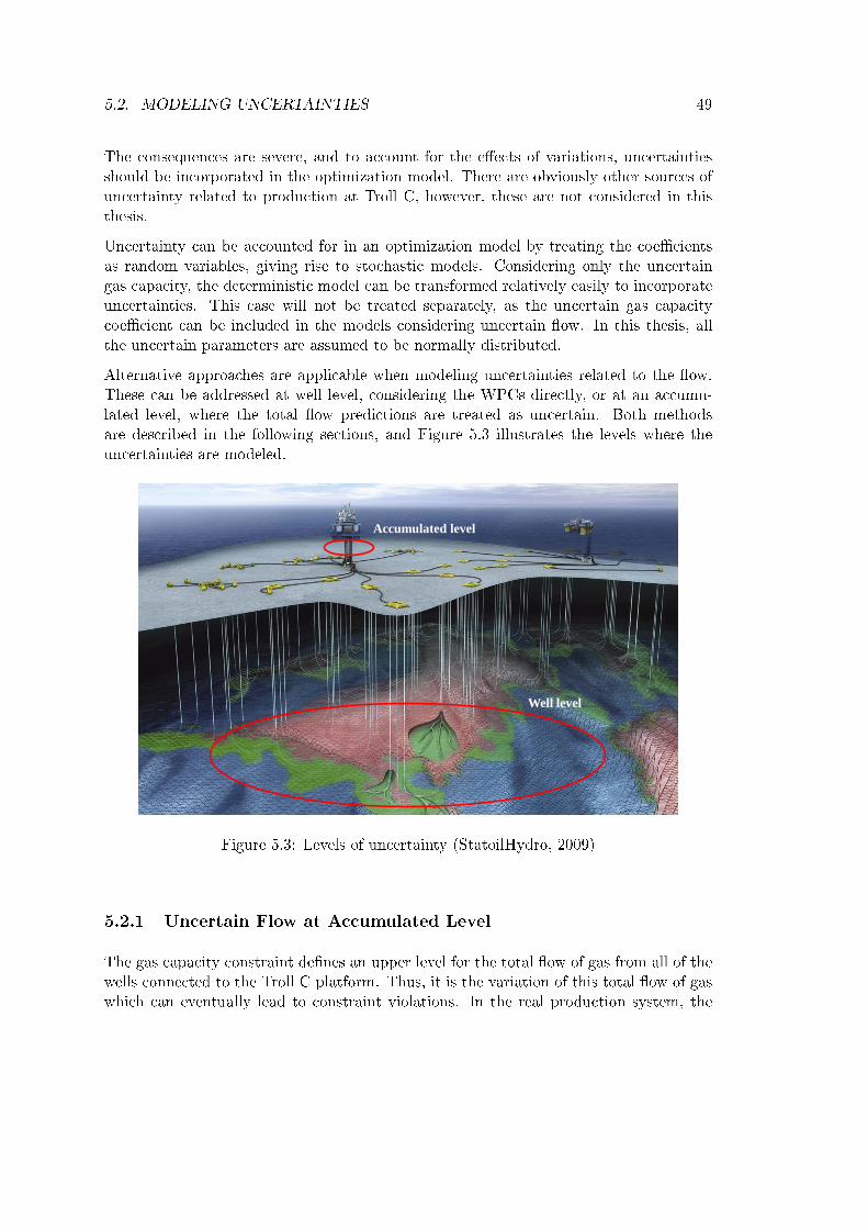
5.2. MODELING UNCERTAINTIES 49
The consequences are severe, and to account for the e�ects of variations, uncertaintiesshould be incorporated in the optimization model. There are obviously other sources ofuncertainty related to production at Troll C, however, these are not considered in thisthesis.
Uncertainty can be accounted for in an optimization model by treating the coe�cientsas random variables, giving rise to stochastic models. Considering only the uncertaingas capacity, the deterministic model can be transformed relatively easily to incorporateuncertainties. This case will not be treated separately, as the uncertain gas capacitycoe�cient can be included in the models considering uncertain �ow. In this thesis, allthe uncertain parameters are assumed to be normally distributed.
Alternative approaches are applicable when modeling uncertainties related to the �ow.These can be addressed at well level, considering the WPCs directly, or at an accumu-lated level, where the total �ow predictions are treated as uncertain. Both methodsare described in the following sections, and Figure 5.3 illustrates the levels where theuncertainties are modeled.
Accumulated level
Well level
Figure 5.3: Levels of uncertainty (StatoilHydro, 2009)
5.2.1 Uncertain Flow at Accumulated Level
The gas capacity constraint de�nes an upper level for the total �ow of gas from all of thewells connected to the Troll C platform. Thus, it is the variation of this total �ow of gaswhich can eventually lead to constraint violations. In the real production system, the

50 CHAPTER 5. UNCERTAINTIES AT TROLL C
wellstreams will adjust to ful�ll the pressure requirements, and the material balances willalways be satis�ed. Anything else is physically impossible. This implies it is possible toassume that all constraints de�ning the physical relations are ful�lled, and consider onlythe resulting total �ow to be uncertain. The gas capacity constraint is accordingly thesole constraint which in reality can be violated as a result of uncertainties. As none ofthe other capacity limits are binding, these will not be a�ected if the production variesslightly. Thus only the deviations in gas �ow need to be considered at this accumulatedlevel.
The varying total gas �ow can be incorporated in the gas capacity constraint presentedbelow:
∑i∈I
AiqPimp ≤ Kp , m = {1} , p = {g} (5.6)
In the deterministic formulation, the coe�cients Ai of the �ow in the pipelines are ob-viously equal to one, as the exact calculated �ow must be included in the constraint.However, treating these coe�cients as random will have the same e�ect as if the �owitself was varying compared to the modeled �ow.
This approach is motivated by Ben-Tal and Nemirovski (1998), arguing that even whensome data of a model is known with certainty, and the corresponding decision variablescan be computed exactly, it is not always possible to implement the solution exactly. Asan example, actual production is often known in advance to deviate from the calculatedvalues of a mathematical model. This is equivalent to having no inaccuracies in theproduction variables, but uncertainties being present in the corresponding parameters(Ben-Tal and Nemirovski, 1998).
The normally distributed random parameters Ai of (5.6) de�ne the uncertainty relatedto the accumulated �ow from each cluster. The mean value is equal to one, implying theexpected production is the same as the calculated �ow, and the degree of uncertainty isspeci�ed by the standard deviation. The uncertainties related to the production fromthe separate clusters are considered to be independent, but this is not a prerequisite inorder to formulate the problem.
5.2.2 Uncertain Flow at Well Level
Treating uncertainty at well level directly in the WPCs results in a more complex model,where the uncertainty must be incorporated in the breakpoints de�ning the piecewiselinear functions. The e�ect is illustrated in Figure 5.4.
The pressure is determined by the operators, but the corresponding �ow may vary aboutthe expected value given by the WPC. Accordingly, only the breakpoints representing

5.2. MODELING UNCERTAINTIES 51
0
400
800
1200
1600
2000
20 30 40 50 60 70 80 90 100
Flow
Pressure
Uncertain WPC
Figure 5.4: E�ect of uncertain WPCs
�ow, QWimjpk, are treated as random variables, not the pressure. As a result, the �owfrom each of the wells is random. This will a�ect the total model, as opposed to in theaccumulated formulation, where only the gas capacity constraint is concerned.
Addressing the WPCs directly gives a more detailed description of the uncertaintiesrelated to the �ow. It is no longer possible to assume that the physical relations areautomatically satis�ed; the required adjustments must be modeled explicitly to observethe e�ects of uncertainty. The �ow of oil and water a�ects the pressure drop, andaccordingly the �ow of all phases. In order to account for the full e�ects of variations onthe gas �ow and the gas capacity constraint, all phases should be treated as uncertainat this level.
The uncertain parameters can be modeled in various ways. As already mentioned, therandom parameters are assumed to be normally distributed, where the degree of un-certainty is measured by the standard deviation. For each of the breakpoints, this canbe given in relative or absolute terms. In this thesis, it is assumed that the standarddeviations are given as a percentage of the mean value for the breakpoint of interest.
It is possible to introduce covariance between the breakpoints of a WPC. If one of thebreakpoints in reality is higher than expected, it may be reasonable to assume that theneighboring points are higher as well. These e�ects can be included when modeling theuncertainty.
The breakpoint for maximum pressure is not considered to be uncertain. This pointde�nes the pressure where the gas, oil, and water �ow equals zero. For modeling purposes,the �ow of all phases must equal zero at the same pressure, thus it is di�cult to includestochasticity in the maximum pressure point. This is evidently a shortcoming, as it ishardly possible to estimate the maximum pressure with certainty.

52 CHAPTER 5. UNCERTAINTIES AT TROLL C
5.3 Stochastic Formulations
The stochastic optimization methods presented in Chapter 3 are both applicable whenmodeling production optimization under uncertainty at Troll C. Recourse and chanceconstrained models have di�erent properties, and the advantages or disadvantages variesdepending on how uncertainties are accounted for. In the following, both methods areapplied to the planning problem, treating uncertain �ow predictions at accumulated andwell level in separate models. The uncertain capacity is also incorporated in the models.In this section, only parts of the problem subject to uncertainty are presented, the totalmodels are given in the next chapter.
5.3.1 Recourse Models with Penalties for Constraint Violations
To avoid damaged equipment, it is essential to keep the gas production level below themaximum limit. In a general recourse model, it is possible to compensate for constraintviolations through the recourse actions at a cost. In the production planning problem,it will be too late to correct potential overproduction in a second stage. Accordingly,there is no recourse action as such, and the recourse variables are merely a measure ofconstraint violations. This is similar to the interpretation of a simple recourse model.By penalizing the recourse variables su�ciently in the objective function, the optimalsolution will be well positioned with respect to avoiding constraint violations.
As described in Chapter 3, recourse problems consist of two stages, where the determin-istic part of the model occurs in the �rst stage problem. The parts of the productionplanning problem subject to uncertainty appear in the second stage of the total model.
Recourse Accumulated Model
When uncertain �ow predictions are treated in the capacity constraint, all the uncertainparameters arise in the same restriction. Both the �ow coe�cients Ai and the capacitylimit Kp are treated as random variables. The resulting constraints are expressed by:
∑i∈I
AiqPimp + y+ − y− ≤ Kp , m = {1}, p = {g} (5.7)
y+, y− ≥ 0 (5.8)
The recourse variable y− measures the constraint violations and should be penalizedin the objective function. In this model, the y+ variable will not have a value whenpenalized, and is only included for completeness. Constraints (5.7) and (5.8) representthe second stage problem of the recourse model. All possible realizations of the uncertain

5.3. STOCHASTIC FORMULATIONS 53
parameters Ai and Kp must be accounted for to obtain the optimal solution to the totalproblem.
This formulation is denoted the recourse accumulated model and incorporates the ac-cumulated uncertainties arising from the total optimization problem. Considerationsregarding pressure and �ow relations through the system when the �ow is uncertain isavoided, which is a major advantage. However, it fails to address the uncertainty atwell level where it arises. The solution obtained will not account for the e�ect of wellswith di�erent uncertainty levels, which may a�ect the production from each well. Theformulation presented in the next section allow for such considerations.
Recourse Well Model
In the following formulation, the uncertain parameters arise both in the WPCs and in thecapacity constraint, which are presented below. This model is referred to as the recoursewell model.
∑i∈I
qPimp + y+ − y− ≤ Kp , m = {1}, p = {g} (5.9)
qWimjp =∑
k∈K(i,m,j)
QWimjpkγimjk , i ∈ I, m ∈M(i), j ∈ J (i,m), p ∈ P (5.10)
y+, y− ≥ 0 (5.11)
The coe�cients Kp and QWimjpk are now the random variables. The recourse variableshave the same interpretation as for the accumulated model. Accounting for the varying�ow directly in the WPCs results in a larger second stage problem, as the pressure dropand material balances must be recalculated for all parameter realizations. In addition tothe recourse variables introduced in the gas capacity restriction, recourse variables mustbe added to the pressure requirement constraints in order to ensure relatively completerecourse. These constraints are presented in the next chapter.
The pipeline �ow in (5.9) is the sum of the �ow from the wells in (5.10), and will varycorresponding to the variations in the WPCs. The e�ect on the capacity constraintwill thus be similar as for the accumulated model presented above. However, treatinguncertainty directly at well level will represent the real system more realistically. Inthis case, it is possible to obtain an optimal solution accounting for di�erent levels ofuncertainty related to the �ow from di�erent wells.
54 CHAPTER 5. UNCERTAINTIES AT TROLL C
5.3.2 Chance Constrained Models Ensuring Safety
In a chance constrained model formulation, constraint violations are avoided applyinga di�erent technique than the recourse models. By demanding the constraints to besatis�ed with at least a given probability, violations are largely prevented.
Chance Constrained Accumulated Model
Treating all uncertainties through the capacity constraint, and applying a chance con-strained model, was proposed for a simpli�ed model by Glæserud and Syrdalen (2008).When modeling uncertain accumulated �ow and capacity limit in a probabilistic con-straint, the following expression is obtained:
Pr
(∑i∈I
AiqPimp ≤ Kp
)≥ η , m = {1}, p = {g} (5.12)
Restating formulation (5.12), the recourse variables of formulation (5.7) are now replacedby a barrier term to prevent the �ow of gas to reach the maximum limit:
∑i∈I
AiqPimp + Φ−1(η)
√∑i∈I
(σAi q
Pimp
)2+ (σK)2 ≤ Kp , m = {1}, p = {g} (5.13)
The parameters Ai, Kp, σAi , and σ
K represent the mean values and standard deviationsof the �ow coe�cients and the capacity limit, respectively. The standard deviationsare the elements of the covariance matrix for the model with uncertain RHS and LHSpresented in Section 3.3.1. In this formulation, the random parameters are assumed tobe independent. The covariance matrix is thus reduced to a diagonal matrix, its elementsrepresenting the variance of the separate parameters. The probability level is given by η,and Φ−1(η) represent the η-quantile of the standard normal distribution. The size of thesecond term, or the barrier term, is dependent on all of these parameters. The dummyvariable introduced in Chapter 3 is omitted in the formulation as it equals one.
The penalized recourse variables of the previously presented models have a similar e�ecton the solution as the barrier term in (5.13). Both elements will reduce the productionto avoid constraint violations. As for the recourse accumulated model, this chance con-strained formulation does not account for well-speci�c uncertainties. The model is calledthe chance constrained accumulated model in the following.

5.3. STOCHASTIC FORMULATIONS 55
Chance Constrained Well Model
Treating uncertain �ow predictions at well level in a chance constrained model is notstraightforward. The resulting formulation, denoted the chance constrained well model,appears to be inappropriate, which is illustrated in the following.
Probabilistic constraints can only be applied to inequality restrictions. As the WPCsin the deterministic model are given by equality relations, these must be transformed inorder to formulate the chance constrained well model. A natural suggestion would beto replace the equality constraint by upper and lower bounds, demanding the estimated�ow to stay within these limits. However, as the gas capacity is binding, it is likelythat the gas �ow will always end up at its lower bound. In this case, the lower boundconstraint will be binding, and the �ow will be the same as with an equality constraint.This suggests the upper bound is redundant, and the original equality constraint can bereplaced with a lower bound inequality constraint.
When solving such reformulated problem, the solution must be investigated to ensurethat the assumption of a binding WPC stated as an inequality constraint holds. Ex-perience indicates that the inequality constraint will indeed be satis�ed with equality.However, other challenges arise when modeling the WPCs as probabilistic constraints.Consider again the WPC relations for gas, where the breakpoints QWimjpk are assumed tobe uncertain:
qWimjp =∑
k∈K(i,m,j)
QWimjpkγimjk , i ∈ I, m ∈M(i), j ∈ J (i,m), p = {g} (5.14)
Transforming (5.14) into inequality constraints, the following is obtained:
qWimjp ≥∑
k∈K(i,m,j)
QWimjpkγimjk , i ∈ I, m ∈M(i), j ∈ J (i,m), p = {g} (5.15)
By stating (5.15) as separate probabilistic constraints, it is demanded with a speci�edprobability that the predicted �ow, qWimjp, must not be underestimated:
Pr
qWimjp ≥ ∑k∈K(i,m,j)
QWimjpkγimjpk
≥ ηimj , i ∈ I, m ∈M(i), j ∈ J (i,m), p = {g}
(5.16)
Transforming (5.16), the following constraint is obtained:

56 CHAPTER 5. UNCERTAINTIES AT TROLL C
qWimjp ≥∑
k∈K(i,m,j)
QWimjpkγimjk + Φ−1(ηimj)
√√√√ ∑k∈K(i,m,j)
(σWimjpkγimjk
)2,
i ∈ I, m ∈M(i), j ∈ J (i,m), p = {g}, (5.17)
where σWimjpk is the standard deviation of breakpoint QWimjpk. The probability of not
underestimating the �ow, qWimjp, is given by ηimj . The barrier term ensures that a highergas �ow than expected is applied in the model, which provides safety with respect toful�lling the gas capacity constraint. However, as the �ow in most cases will be lower thanthe overestimated qWimjp, the pressure drop calculations are in reality no longer correct.Modi�cations are thus necessary to obtain valid pressure relations. Including uncertain�ow of oil and water will further complicate these adjustments.
The constraints in (5.16) are imposed for every well, giving rise to a conservative model.As all of the wells are required to overestimate the �ow most of the time, the total actual�ow will be lower than necessary with respect to the capacity constraint.
The di�culties arising when developing the chance constrained well model indicate thatthis formulation is inappropriate for the production planning problem at Troll C. Accord-ingly, only the recourse and chance constrained accumulated models and the recourse wellmodel are presented in the next chapter.

Chapter 6
Stochastic Models
The previous chapter investigates and presents several alternatives for incorporating un-certainty in the production optimization problem at the Troll C �eld. In this chapter,the complete models of the suggested formulations are given. Section 6.1 provides ad-ditional assumptions and simpli�cations required for the stochastic models, whereas therecourse models and the chance constrained model are presented in Sections 6.2 and 6.3,respectively.
6.1 Additional Assumptions and Simpli�cations
In stochastic optimization models, uncertainties are incorporated by treating some of theparameters as random variables. At Troll C, there is currently no information availabledescribing the distribution of uncertain coe�cients, thus normally distributed param-eters are assumed. This is a better approximation compared to �xed parameters, asStatoilHydro con�rms uncertainty related to both estimated production levels and thegas capacity limit.
Uncertain �ow predictions, resulting from complex WPC modeling, and varying gascapacity, are the sole uncertainties incorporated in the models presented in this chapter.There are obviously other sources of uncertainty related to the production at Troll C, forexample the approximate pressure drop models. However, in order to obtain optimizationproblems of reasonable size, these uncertainties are not considered any further.
All the assumptions and simpli�cations presented for the deterministic problem in Chap-ter 4 apply to the stochastic models as well.
57
58 CHAPTER 6. STOCHASTIC MODELS
6.2 Formulation of the Recourse Models
In the following sections, the two recourse formulations introduced in Chapter 5 are pre-sented in detail. The models incorporate uncertainties related to both the �ow estimatesand the gas capacity limit. As there are multiple uncertain parameters in some of theconstraints, nonlinear solution methods are not appropriate. Discretization and samplingare applied to solve the problems; accordingly the second stage of the models presentedconsists of scenarios representing the outcomes of the uncertain parameters.
6.2.1 Recourse Accumulated Model
In the previous chapter it is argued that both the gas capacity limit and the �ow of gasfrom the clusters are uncertain. The following model incorporates all these uncertaintiesin the gas �ow capacity restriction, as proposed in Section 5.3.1. This model containsonly three random parameters, which implies it is possible to discretize the distributionfunctions with a satisfactorily accuracy, without ending up with a too large problem.
Additional Declarations for the Recourse Accumulated Formulation
The recourse models are extensions of the deterministic model presented in Chapter 4,thus only the additional declarations needed to incorporate uncertainties are presentedin the following. The random parameters and variables are denoted by a superscript Rto separate the random and the deterministic parameters, and the additional index s torepresent the scenario. All the �rst stage variables and parameters are already declaredin the deterministic model, see Chapter 4.
Indices
s Scenario
Sets
S Set of scenarios
Data
CK+ Unit cost of gas capacity surplus
CK− Unit cost of gas capacity shortage
ARis Coe�cient representing uncertain accumulated �owfrom cluster i in scenario s

6.2. FORMULATION OF THE RECOURSE MODELS 59
KRs Uncertain gas capacity limit in the �rst stage separator at platform level in
scenario s
Variables
y+s Surplus variable for gas capacity constraint in scenario s
y−s Shortage variable for gas capacity constraint in scenario s
In the recourse accumulated model, the only second stage parameters and decision vari-ables occur in the gas capacity restriction, which forms the second stage problem. Allthe other constraints and decisions belong to the �rst stage, and are identical to the de-terministic restrictions. These constraints and corresponding parameters are presentedin the following without explanations, and the reader is referred to Chapter 4 for thecomplete description.
Objective Function
The objective in the recourse accumulated model is the same as in the deterministicformulation; to maximize oil produced. In addition, the recourse shortage and surplusvariables must be included along with the corresponding costs. The expected value ofthe costs of the recourse actions are calculated based on all scenario realizations, and isgiven by the two last terms of (6.1).
max Z =∑i∈I
qPimp −1|S|∑s∈S
CK+y+s −
1|S|∑s∈S
CK−y−s , m = {1}, p = {o} (6.1)
First Stage Constraints
The constraints of the �rst stage problem are not subject to uncertainty, and are thesame as in the deterministic problem. As discussed in the previous chapter, the watercapacity constraint is not binding, and will not be a�ected by uncertain �ow estimates.For simplicity, it is thus omitted from this formulation.
Well Performance Curves
pWimj =∑
k∈K(i,m,j)
PWimjkγimjk , i ∈ I, m ∈M(i), j ∈ J (i,m) (6.2)

60 CHAPTER 6. STOCHASTIC MODELS
qWimjp =∑
k∈K(i,m,j)
QWimjpkγimjk , i ∈ I, m ∈M(i), j ∈ J (i,m), p ∈ P (6.3)
∑k∈K(i,m,j)
γimjk = 1 , i ∈ I, m ∈M(i), j ∈ J (i,m) (6.4)
γimjk is SOS2 , i ∈ I, m ∈M(i), j ∈ J (i,m) (6.5)
Material Balances
qPimp =∑
j∈J (i,m)
qWimjp + qPi(m+1)p , i ∈ I, m 6∈ max{M(i)} , p ∈ P (6.6)
qPimp =∑
j∈J (i,m)
qWimjp , i ∈ I, m ∈ max{M(i)} , p ∈ P (6.7)
Pressure Drop Curves
pDim =∑p∈P
DFimpq
Pimp +DC
im , i ∈ I, m ∈M(i) (6.8)
Pressure Balances
pMi(m−1) = pMim − pDim , i ∈ I, m 6= {1} (6.9)
PS = pMim − pDim , i ∈ I , m = {1} (6.10)
Pressure Requirement
pMim ≤ pWimj +(PMAXi − PWMX
imj
)(1− ximj) , i ∈ I, m ∈M(i), j ∈ J (i,m) (6.11)
Closing Wells
qWimjp ≤ QMAXimjp ximj , i ∈ I, m ∈M(i), j ∈ J (i,m), p ∈ P (6.12)

6.2. FORMULATION OF THE RECOURSE MODELS 61
Variable Requirements
qPimp ≥ 0 , i ∈ I, m ∈M(i), p ∈ P (6.13)
pWimj ≥ PMIN , i ∈ I, m ∈M(i), j ∈ J (i,m) (6.14)
qWimjp ≥ 0 , i ∈ I, m ∈M(i), j ∈ J (i,m), p ∈ P (6.15)
γimjk ≥ 0 , i ∈ I, m ∈M(i), j ∈ J (i,m), k ∈ K(i,m, j) (6.16)
pDim ≥ 0 , i ∈ I, m ∈M(i) (6.17)
pMim ≥ 0 , i ∈ I, m ∈M(i) (6.18)
ximj ∈ {0, 1} , i ∈ I, m ∈M(i), j ∈ J (i,m) (6.19)
Second Stage Constraints
The uncertain parameters and the recourse variables are scenario-dependent, and occurin the second stage problem. The constraints representing the second stage problem aregiven in the following.
Gas Flow Capacity The gas �ow capacity limit is considered to be uncertain, denotedby the scenario-dependent KR
s . In order to incorporate the e�ect of uncertain gas �ow,the coe�cients ARis of the �ow variables from the clusters are treated as random. Thesecond stage variable y−s is incorporated to ensure feasibility, and to capture the amountof possible deviations from the capacity limit. For completeness, y+
s is included, but willnot take a value when penalized in the objective function.
∑i∈I
ARisqPimp + y+
s − y−s ≤ KRs , m = {1}, p = {g}, s ∈ S (6.20)
Variable Requirements The recourse variables must be positive, and the non-negativityrequirements are given by (6.21).
y+s , y
−s ≥ 0 , s ∈ S (6.21)
The recourse accumulated model represents the uncertainties in the model parametersby a large number of scenarios, where all possible combinations of parameter realizationsare included in the second stage problem. The resulting problem is thus a large scaleextension of the deterministic MILP model.

62 CHAPTER 6. STOCHASTIC MODELS
6.2.2 Recourse Well Model
As described in Chapter 5, the uncertainties related to the predicted �ow can either becompensated for in the capacity constraint, or directly in the well models. The latterformulation is presented in the following, introducing stochastic breakpoints for the �owdescribed by the WPCs.
Modeling uncertain breakpoints gives a more complex model compared to the accu-mulated formulation presented above, as more constraints and variables are scenario-dependent. The number of random parameters is increased, resulting in a large scaleproblem. To reduce the problem size, the sample average approximation solution methodis applied, and the second stage is thus represented by scenarios.
Additional Declarations for the Recourse Well Formulation
The scenario-dependent parameters and variables are represented by the superscript Rand the additional index s, as for the recourse accumulated model. The additionaldeclarations needed to present the recourse well model are given in the following.
Indices
s Scenario
Sets
S Set of scenarios
Data
CK+ Unit cost of gas capacity surplus
CK− Unit cost of gas capacity shortage
CP+imj Unit cost of pressure requirement surplus
CP−imj Unit cost of pressure requirement shortage
KRs Uncertain gas capacity limit in the �rst stage separator at platform level in
scenario s
QWRimjpks Breakpoint k of the uncertain piecewise linear WPC for �ow rate of phase p
from well j, manifold m, cluster i, in scenario s
QMAXRimjps Maximum �ow of phase p from well j, manifold m,
cluster i, in scenario s

6.2. FORMULATION OF THE RECOURSE MODELS 63
Variables
qPRimps Flow rate of phase p from manifold m to manifold
(m− 1) or separator in cluster i, scenario s
y+s Surplus variable for gas capacity constraint in scenario s
y−s Shortage variable for gas capacity constraint in scenario s
w+imjs Surplus variable for pressure requirement constraint for well j,
manifold m, cluster i, in scenario s
w−imjs Shortage variable for pressure requirement constraint for well j,
manifold m, cluster i, in scenario s
qWRimjps Flow rate of phase p from well j, manifold m, cluster i, in scenario s
pDRims Pressure drop for �ow from manifold m to manifold (m− 1) or theseparator in cluster i, scenario s
pMRims Pressure at manifold level for �ow from manifold m in
cluster i, scenario s
The only �rst stage decisions are the pressure levels in each well, and the correspondingwell closing decision. The �ow of gas, oil, and water from the wells is random, thus allvariables and constraints related to this �ow are scenario-dependent, and form the secondstage problem.
Objective Function
Maximization of oil production is again the objective of the model. In this formulation,the total objective function is scenario-dependent, and represented by expected values.The recourse costs capturing pressure requirement deviations are included, in additionto the costs of the capacity constraint deviations.
max Z =1|S|∑i∈I
∑s∈S
qPRimps −1|S|∑s∈S
CK+y+s −
1|S|∑s∈S
CK−y−s
− 1|S|∑s∈S
CP+imjw
+imjs −
1|S|∑s∈S
CP−imjw−imjs , m = {1}, p = {o} (6.22)
First Stage Constraints
The �rst stage constraints represent the deterministic part of the problem, and are givenin the following.
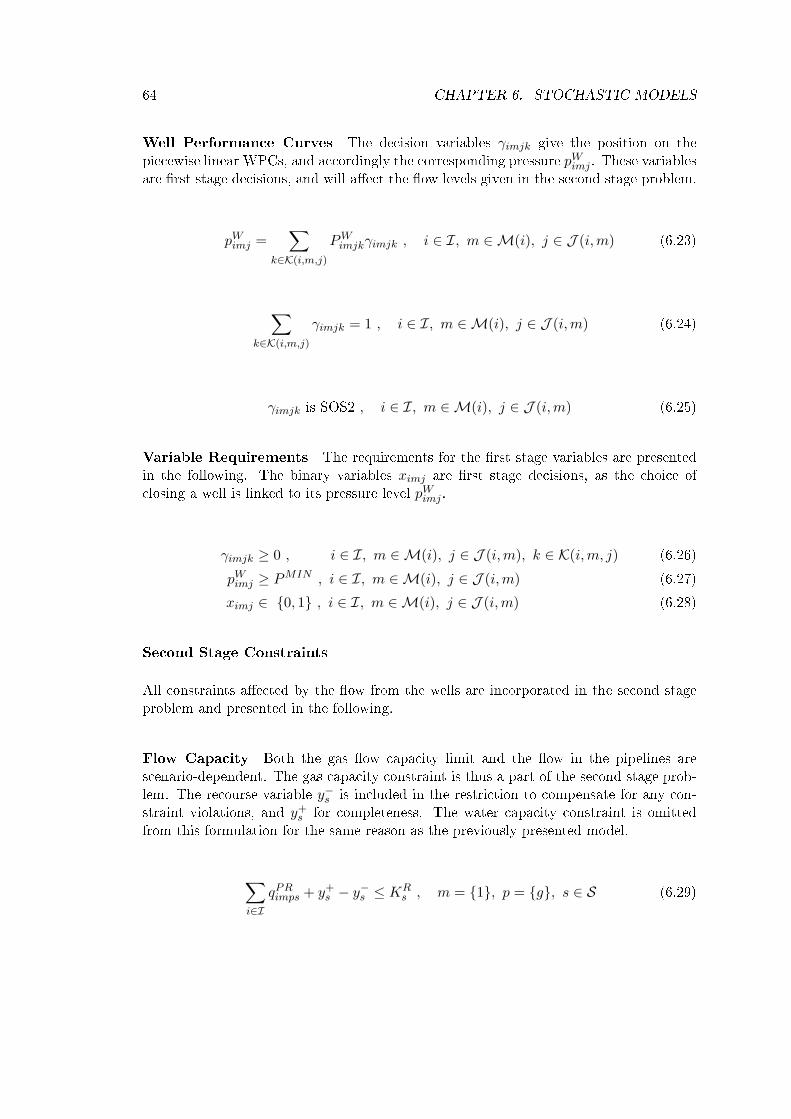
64 CHAPTER 6. STOCHASTIC MODELS
Well Performance Curves The decision variables γimjk give the position on thepiecewise linear WPCs, and accordingly the corresponding pressure pWimj . These variablesare �rst stage decisions, and will a�ect the �ow levels given in the second stage problem.
pWimj =∑
k∈K(i,m,j)
PWimjkγimjk , i ∈ I, m ∈M(i), j ∈ J (i,m) (6.23)
∑k∈K(i,m,j)
γimjk = 1 , i ∈ I, m ∈M(i), j ∈ J (i,m) (6.24)
γimjk is SOS2 , i ∈ I, m ∈M(i), j ∈ J (i,m) (6.25)
Variable Requirements The requirements for the �rst stage variables are presentedin the following. The binary variables ximj are �rst stage decisions, as the choice ofclosing a well is linked to its pressure level pWimj .
γimjk ≥ 0 , i ∈ I, m ∈M(i), j ∈ J (i,m), k ∈ K(i,m, j) (6.26)
pWimj ≥ PMIN , i ∈ I, m ∈M(i), j ∈ J (i,m) (6.27)
ximj ∈ {0, 1} , i ∈ I, m ∈M(i), j ∈ J (i,m) (6.28)
Second Stage Constraints
All constraints a�ected by the �ow from the wells are incorporated in the second stageproblem and presented in the following.
Flow Capacity Both the gas �ow capacity limit and the �ow in the pipelines arescenario-dependent. The gas capacity constraint is thus a part of the second stage prob-lem. The recourse variable y−s is included in the restriction to compensate for any con-straint violations, and y+
s for completeness. The water capacity constraint is omittedfrom this formulation for the same reason as the previously presented model.
∑i∈I
qPRimps + y+s − y−s ≤ KR
s , m = {1}, p = {g}, s ∈ S (6.29)

6.2. FORMULATION OF THE RECOURSE MODELS 65
Well Performance Curves The breakpoints of the WPCs are scenario-dependent,while γimjk are �rst stage variables, and have the same values in all scenarios. Theresulting �ow will vary depending on the given scenario, and qWR
imjps are thus second stagevariables.
qWRimjps =
∑k∈K(i,m,j)
QWRimjpksγimjk , i ∈ I, m ∈M(i), j ∈ J (i,m), p ∈ P, s ∈ S
(6.30)
Material Balances The accumulated production level is the sum of the scenario-dependent �ow from the wells. Accordingly, the material balance constraints are alsoscenario-dependent, given by (6.31) and (6.32).
qPRimps =∑
j∈J (i,m)
qWRimjps + qPRi(m+1)ps , i ∈ I, m 6∈ max{M(i)}, p ∈ P, s ∈ S (6.31)
qPRimps =∑
j∈J (i,m)
qWRimjps , i ∈ I, m ∈ max{M(i)}, p ∈ P, s ∈ S (6.32)
Pressure Drop Curves The pressure drop through the pipelines is dependent on the�ow of all phases, and is uncertain due to the scenario-dependent qPRimps. It is thus a partof the second stage problem.
pDRims =∑p∈P
DFimpq
PRimps +DC
im , i ∈ I, m ∈M(i), s ∈ S (6.33)
Pressure Balances In all scenarios, the pressure balances must be ful�lled. Theseconstraints are scenario-dependent as the pressure drop in (6.33) varies.
pMRi(m−1)s = pMR
ims − pDRims , i ∈ I, m 6= {1}, s ∈ S (6.34)
PS = pMRims − pDRims , i ∈ I, m = {1}, s ∈ S (6.35)

66 CHAPTER 6. STOCHASTIC MODELS
Pressure Requirement The possibility to close down a well to avoid pressure require-ments is a �rst stage decision. However, as the pressure levels involved are dependent onscenario, the pressure requirement constraint is incorporated in the second stage prob-lem. Note the additional recourse variables w+
imjs and w−imjs, where w
−imjs are included
in (6.36) to ensure relatively complete recourse, and w+imjs for completeness.
pMRims + w+
imjs − w−imjs ≤ p
Wimj +
(PMAXi − PWMX
imj
)(1− ximj) ,
i ∈ I, m ∈M(i), j ∈ J (i,m), s ∈ S (6.36)
Closing Wells A well is allowed to produce up to its maximum �ow level, if it is notclosed to avoid the pressure requirements of (6.36). The maximum �ow level is dependenton the WPC of a given scenario, and the following constraints are parts of the secondstage problem.
qWRimjps ≤ QMAXR
imjps ximj , i ∈ I, m ∈M(i), j ∈ J (i,m), p ∈ P, s ∈ S (6.37)
Variable Requirements The variable requirements for the second stage variables arepresented below.
y+s , y
−s ≥ 0 , s ∈ S (6.38)
w+imjs, w
−imjs ≥ 0 , i ∈ I, m ∈M(i), j ∈ J (i,m), s ∈ S (6.39)
qPRimps ≥ 0 , i ∈ I, m ∈M(i), p ∈ P, s ∈ S (6.40)
qWRimjps ≥ 0 , i ∈ I, m ∈M(i), j ∈ J (i,m), p ∈ P, s ∈ S (6.41)
pDRims ≥ 0 , i ∈ I, m ∈M(i), s ∈ S (6.42)
pMRims ≥ 0 , i ∈ I, m ∈M(i), s ∈ S (6.43)
The recourse well model is a large scale MILP as the recourse accumulated model. Thereare more uncertain parameters in the well model, however, these are represented bysampling rather than discretization of the uncertain parameters, to control the problemsize.
6.3 Formulation of the Chance Constrained Model
Chance constrained programming is appropriate when uncertainty related to the �owpredictions is treated at an accumulated level. The resulting model accounts for both

6.3. FORMULATION OF THE CHANCE CONSTRAINED MODEL 67
varying �ow and uncertain gas capacity limit and is presented in the following sections.
6.3.1 Chance Constrained Accumulated Model
In Chapter 5, the importance of not violating the gas capacity constraint is empha-sized. When the accumulated �ow is known to deviate from the modeled value, thesevariations must be taken into account to avoid exceeding the capacity limit. The sameapproach as for the recourse accumulated model is applied in the following, treating the�ow coe�cients of the gas capacity constraint as random parameters. By introducing aprobabilistic gas capacity constraint, the chance of having overproduction of gas can becontrolled.
Additional Declarations for the Chance Constrained Formulation
The uncertain coe�cients are assumed to be normally distributed, and the parameters ofthe distribution function appear in the probabilistic constraints. The following additionaldeclarations are thus necessary to present the chance constrained model.
Data
Ai Mean value of the random �ow coe�cient ARi for cluster i
σAi Standard deviation of the random �ow coe�cient ARi for cluster i
K Mean value of the random capacity limit KR
σK Standard deviation of the gas capacity limit KR
η Probability level de�ning the minimum probability of not violatingthe gas capacity constraint
The only di�erence between the chance constrained and the deterministic model is theprobabilistic gas capacity constraint. However, the total problem formulation is providedfor completeness. The constraints and parameters familiar from the deterministic prob-lem are not commented, and the reader is referred to Chapter 4 for the full description.
Objective Function
max Z =∑i∈I
qPimp , m = {1}, p = {o} (6.44)

68 CHAPTER 6. STOCHASTIC MODELS
Gas Flow Capacity The gas �ow coe�cients and the gas capacity limit are consideredto be uncertain, and are incorporated in a chance constraint. Imposing the probabilisticconstraint results in a more restrictive problem compared to the deterministic formula-tion. The second term of (6.45) can be interpreted as a barrier, reducing the chance ofconstraint violations.
∑i∈I
AiqPimp + Φ−1(η)
√∑i∈I
(σAi q
Pimp
)2+ (σK)2 ≤ K , m = {1}, p = {g} (6.45)
The parameter Φ−1(η) is the η-quantile of standard normal distribution. The barrierterm is dependent on the standard deviations σAi and σK of the uncertain coe�cients,and the selected probability η of not exceeding the capacity limit. When the uncertaintylevel grows, or the minimum probability of avoiding constraint violations is increased,constraint (6.45) will be more restrictive, reducing the objective value. The water capac-ity is not included in equation (6.45), as it is not binding today. A barrier term wouldthus not a�ect the solution, and the water capacity constraint can be omitted.
Well Performance Curves
pWimj =∑
k∈K(i,m,j)
PWimjkγimjk , i ∈ I, m ∈M(i), j ∈ J (i,m) (6.46)
qWimjp =∑
k∈K(i,m,j)
QWimjpkγimjk , i ∈ I, m ∈M(i), j ∈ J (i,m), p ∈ P (6.47)
∑k∈K(i,m,j)
γimjk = 1 , i ∈ I, m ∈M(i), j ∈ J (i,m) (6.48)
γimjk is SOS2 , i ∈ I, m ∈M(i), j ∈ J (i,m) (6.49)
Material Balances
qPimp =∑
j∈J (i,m)
qWimjp + qPi(m+1)p , i ∈ I, m 6∈ max{M(i)} , p ∈ P (6.50)
qPimp =∑
j∈J (i,m)
qWimjp , i ∈ I, m ∈ max{M(i)} , p ∈ P (6.51)

6.3. FORMULATION OF THE CHANCE CONSTRAINED MODEL 69
Pressure Drop Curves
pDim =∑p∈P
DFimpq
Pimp +DC
im , i ∈ I, m ∈M(i) (6.52)
Pressure Balances
pMi(m−1) = pMim − pDim , i ∈ I, m 6= {1} (6.53)
PS = pMim − pDim , i ∈ I , m = {1} (6.54)
Pressure Requirement
pMim ≤ pWimj +(PMAXi − PWMX
imj
)(1− ximj) , i ∈ I, m ∈M(i), j ∈ J (i,m) (6.55)
Closing Wells
qWimjp ≤ QMAXimjp ximj , i ∈ I, m ∈M(i), j ∈ J (i,m), p ∈ P (6.56)
Variable Requirements
qPimp ≥ 0 , i ∈ I, m ∈M(i), p ∈ P (6.57)
pWimj ≥ PMIN , i ∈ I, m ∈M(i), j ∈ J (i,m) (6.58)
qWimjp ≥ 0 , i ∈ I, m ∈M(i), j ∈ J (i,m), p ∈ P (6.59)
γimjk ≥ 0 , i ∈ I, m ∈M(i), j ∈ J (i,m), k ∈ K(i,m, j) (6.60)
pDim ≥ 0 , i ∈ I, m ∈M(i) (6.61)
pMim ≥ 0 , i ∈ I, m ∈M(i) (6.62)
ximj ∈ {0, 1} , i ∈ I, m ∈M(i), j ∈ J (i,m) (6.63)
The problem size of the chance constrained problem will be smaller than the correspond-ing recourse accumulated formulation, where the random elements are represented bya large number of scenarios. The chance constrained model is a mixed integer nonlin-ear problem (MINLP), which in general can be di�cult to solve to global optimality.However, as described in Chapter 3, the nonlinear probabilistic constraint is convex fornormally distributed parameters. The MINLP is thus convex if the binary variables arerelaxed, which can be exploited when solving the problem.

70 CHAPTER 6. STOCHASTIC MODELS

Chapter 7
Implementation
The previous chapters indicate solving recourse and chance constrained models can bedemanding. The computational requirements of the proposed models are discussed inSection 7.1, while a presentation of appropriate software is given in Section 7.2, withemphasis on the solvers selected for the problems presented. The implementation of themodels is described in Section 7.3, while the processing of results is presented in Section7.4.
7.1 Computational Requirements
The deterministic model for the optimization problem at Troll C is a mixed integer linearprogram (MILP). The binary variables for well closing, and possibly the SOS2 formula-tions, require solvers with algorithms for integer problems. The branch and bound (B&B)method is the most successful algorithm so far, and is implemented in almost all com-mercial solvers for mixed integer problems (Williams, 1999). The structure of the SOS2sets can also be exploited within the B&B algorithm to gain computational advantages.The reader is referred to Rardin (1998) for a description of the B&B algorithm.
For the recourse models presented in Chapter 6, discretization and sampling are consid-ered to be the most appropriate solution methods. When applying these approximations,the MILP structure of the deterministic formulation remains. However, as the number ofoutcomes for each parameter in the discretization grows, the number of variables in themodel increases exponentially. The sample average approximation (SAA) method alsorequires a large number of scenarios to converge to the true optimal solution. Large-scalemixed integer linear optimization tools are thus required to solve the models, of whichthere exist several o�-the-shelf products.
Reformulating the deterministic model into a chance constrained model, a mixed integernonlinear program (MINLP) results. As described in Chapter 3, the barrier term of
71

72 CHAPTER 7. IMPLEMENTATION
the probabilistic constraints gives rise to a second order cone program (SOCP). This is anonlinear problem, thus MILP solvers can no longer be applied, and the set of appropriatesoftware is reduced. The problem is convex when the integrality requirements are relaxed,a property which can be exploited in a B&B framework. Accordingly, the problem canbe solved to global optimality. The chance constrained model proposed in the previouschapter thus require solvers combining nonlinear methods and B&B techniques.
7.2 Choice of Software
The models presented in Chapter 6 require both MILP and MINLP solvers. Various soft-ware packages exist, and a motivation for the choice of software is given in the following.
7.2.1 Mixed Integer Linear Program Solvers
XpressMP from Dash Optimization is a software system solving linear, continuous, inte-ger, and mixed-integer programs by applying a sophisticated B&B algorithm with linearrelaxations (Ashford, 2007). For the deterministic and recourse problems, XpressMP isfound the most suitable software. The models contain special ordered sets, which canbe treated e�ciently by XpressMP. When declaring the variables to be of SOS2 type,XpressMP recognizes the SOS2 structure during the presolve procedure (Ashford, 2007),and branches on sets of variables instead of variables in the B&B tree (Guéret et al.,2007).
The XpressMP product suite is presented in Figure 7.1. The mathematical problems areformulated in the Mosel language, which is a high-level language allowing for formulationsclose to the algebraic notation (Dash Optimization, 2007). Xpress-IVE provides a visualuser interface, enabling for example graphical displays of solutions and runtime statistics.In this thesis, the MILP solver Xpress-Optimizer is applied, using the mmxprs library.The complete version of XpressMP is needed to solve the recourse problems, due to thelarge number of variables and constraints.
The e�cient treatment of SOS2 variables is the main reason for selecting XpressMP asthe solver for the MILPs. The complete version is available at the Norwegian Universityof Science and Technology (NTNU) where this thesis is written, further encouraging thischoice of software.
7.2.2 Mixed Integer Non-Linear Program Solvers
Prior to the work of this master thesis, no MINLP solvers were easily available at NTNU,necessitating a more thorough evaluation of appropriate software. A short presentationof some of the relevant software is given in the following.

7.2. CHOICE OF SOFTWARE 73
Figure 1.2: Xpress-MP product suite
This facility may be useful for embedding the Optimizer into applications that possesstheir own, dedicated matrix generation routines.Advanced Xpress users may wish to employ special features of the Optimizer that arenot available through the different interfaces, possibly using a matrix that has previouslybeen generated by Mosel or BCL.
Of the three above mentioned approaches, a high-level language certainly provides the easiest-to-understand access to Mathematical Programming. So in the first and largest part of thisbook we show how to define and solve problems with the Xpress-Mosel language, and alsohow the resulting models may be embedded into applications using the Mosel libraries. Wework with Mosel models in the graphical user interface Xpress-IVE, exploiting its facilities fordebugging and solution analysis and display.
In the reminder of this book we show how to formulate and solve Mathematical Programmingproblems directly in a programming language environment. This may be done with modelingsupport from BCL or directly using the Xpress-Optimizer library. With BCL, models can beimplemented in a form that is relatively close to their algebraic formulation and so are quiteeasy to understand and to maintain. We discuss BCL implementations of the same exampleproblems as used with Mosel.
The last part of this book explains how problems may be input directly into the Optimizer, ei-ther in the form of matrices (possibly generated by another tool such as Mosel or BCL) that areread from file, or by specifying the problem matrix coefficient-wise directly in the applicationprogram. The facility of working directly with the Optimizer library is destinated at embeddersand advanced Xpress-MP users. It is not recommendable as a starting point for the novice inMathematical Programming.
1.2.1 Note on product versions
All examples in this book have been developed using the Xpress-MP Release 2007A (Mosel2.0.0, IVE 1.17.2, BCL 3.0.1, Optimizer 17.0.2). If they are run with other product versions theoutput obtained may look different. In particular, improvements to the algorithms or modifi-cations to the default settings in Xpress-Optimizer may influence the behavior of the LP searchor the shape of the MIP branching trees. The IVE interface may also undergo slight changes infuture releases as new features are added, but this will not affect the actions described in thisbook.
Introduction 6 Getting started
Figure 7.1: Xpress-MP product suite (Dash Optimization, 2007)
The NEOS server is an on-line server which gives free access to state-of-the-art optimiza-tion solvers (NEOS server, 2009). The user chooses an appropriate solver and submitsoptimization problems and data to the server. The NEOS server links the submittedmodel with the solver, and returns the solution and runtime statistics (Czyzyk et al.,1998). For the purpose of testing various solvers on optimization problems, the NEOSserver can be a useful tool.
In Glæserud and Syrdalen (2008), a chance constrained model for the optimizationproblem at Troll C is solved by using the open-source toolbox, YALMIP, run throughMATLAB R©. YALMIP provides both a modeling language and simple solvers for ad-vanced optimization problems, where additional external open-source solvers can be in-stalled to increase the performance of the toolbox (Löfberg, 2004). One of these is theSDPT3 solver, which applies interior point methods for solving conic problems. Glæserudand Syrdalen (2008) present a small problem compared to the model proposed in thisthesis, and argue that YALMIP is only suitable for small size problems. YALMIP is thusnot considered appropriate in this thesis.
Bonmin (Basic Open- Source Nonlinear Mixed Integer programming) is a special purposesolver for MINLPs, developed by researchers at IBM and Carnegie Mellon University,and distributed through COIN-OR (COmputational INfrastructure for Operations Re-search). COIN-OR is an open-source community aiming to speed up the computationaldevelopment within mathematical programming (Lougee-Heimer, 2003). For further in-formation about Bonmin and COIN-OR, the reader is referred to Bonami and Lee (2007)and COIN-OR (2009).
The Branch-and-Reduce Optimization Navigator (BARON) solves MINLPs to global op-timality. In a recent computational study of global solvers by Neumaier et al. (2005),BARON is stated as the fastest and most robust solver among the available solvers. It isthus chosen as the MINLP solver in this thesis. BARON implements the B&B algorithmenhanced with several techniques for increasing its e�ciency (Sahinidis and Tawarmalani,2005). However, there is no special treatment of SOS2 sets, and these requirements mustbe formulated explicitly.

74 CHAPTER 7. IMPLEMENTATION
BARON is available under the programming languages AIMMS or GAMS, where GAMSis preferred in this thesis. GAMS, or General Algebraic Modeling System, is a high-levelmodeling system for optimization and mathematical programming. GAMS is designedto solve large and complex linear, nonlinear, and mixed integer problems. A graphicalinterface which allows for editing, developing, debugging, and running GAMS models isprovided by GAMS IDE (Integrated Development Environment) (McCarl, 2008).
The GAMS/BARON system requires access to both linear and nonlinear programmingsolvers. It is possible to choose among the linear solvers CPLEX, MINOS, SNOPT,XA, and Xpress, and the nonlinear solvers MINOS and SNOPT. MINOS is preferred inthis thesis as it is chosen by default as the nonlinear solver in BARON. MINOS solvesnonlinear problems with the augmented Lagrangian method and the reduced gradientmethod described in Chapter 3. The interface between GAMS, BARON, and othersolvers is shown in Figure 7.2.
GAMS ModelsGAMS Models
NLP, DNLP, MINLP
ModelInput
GlobalSolution
BARON
PreprocessorPreprocessorBranch and Reduce
Heuristics
Convex Relaxations / Local Search
GAMS/CPLEX
GAMS/MINOS
GAMS/SNOPT
Figure 7.2: GAMS/BARON interface (GAMS Home Page, 2009)
The optimization model is implemented in GAMS IDE, linking the problem to the solver.The preprocessor is started, and the branch and reduce algorithm is run while MINOSsolves the linear and/or nonlinear problems. For more information about GAMS andBARON, the reader is referred to Sahinidis and Tawarmalani (2005) and McCarl (2008).
7.3 Implementation of the Models
One of the advantages of programming in high-level modeling languages as Mosel andGAMS is the similarities between the syntax and the mathematical structure of optimiza-

7.3. IMPLEMENTATION OF THE MODELS 75
tion problems. In this thesis, all the data for the various models are given in separate �les.The complete implementation of the models are presented in the electronic Appendix C.
The deterministic model presented in Chapter 4 is implemented as a benchmark in bothXpressMP and GAMS. The SOS2 must be modeled explicitly in GAMS/BARON, whilethe makesos2 procedure can be used in XpressMP, which simpli�es the model formulation.
The recourse accumulated model and the well model presented in Chapter 6 are imple-mented in XpressMP. Parameter input is given by various data-�les (.dat), as illustratedin Figure 7.3. For the recourse accumulated model, the normally distributed randomparameters are discretized. The probability density function is divided into an appropri-ate number of intervals, where the expected value of each interval represents a discreteoutcome for the given parameter. The intervals are chosen so as the probabilities of alloutcomes are the same. The expected values of the intervals are calculated by numericalintegration in MATLAB R©. All combinations of outcomes for the random parametersrepresent the scenarios of the problem, and are provided as input to XpressMP in .datformat. The extensive form of the resulting problem is then solved directly. The fulldescription of the discretization procedure is given in Appendix A.
Stochastic Models
Chance Constrained Recourse ModelsData Files (.dat) Data Files (.xls)Model
(GAMS)
Recourse Models(XpressMP)
WellAccumulated AccumulatedWell
SAA(Matlab .dat)
Discretize(Matlab .dat)
Direct(Excel .xls)
Processing f
( )( )
ofResults
Excel(.xls)
Figure 7.3: File structure of the stochastic models
The recourse well model contains a larger number of uncertain parameters than theaccumulated model. It is solved by the sample average approximation method (SAA),presented in Chapter 3. SAA is a statistical method, where the scenarios representing theoutcomes of the uncertain parameters are randomly generated. The simulated scenariosare generated in MATLAB R©, and exported to a .dat-�le, which is provided as input toXpressMP.
The solution of the SAA-problem is based on N scenarios for the uncertain parametersof the recourse well model. The lower limit for the optimality gap of this SAA solution

76 CHAPTER 7. IMPLEMENTATION
is obtained by inserting and �xing the optimal �rst stage variables in the same recoursemodel, with a larger number of scenarios, N ′. The upper limit of the gap is calculated asthe average of M solutions with N scenarios, obtained by solving the M SAA problemsin a loop. The variances and con�dence levels for the upper and lower limits of theoptimality gap are calculated in Excel.
In order to calculate the value of the stochastic solution, the the expected value of theexpected value solution (EEV) is needed for both recourse models. This is obtainedby inserting the expected value (EV) solution into the stochastic XpressMP model as a�rst stage decision, where the resulting second stage problem is optimized. The VSS iscalculated in Excel as the di�erence between EEV and the optimal objective value fromthe stochastic solution.
The expected value of perfect information can be found by calculating the wait-and-see(WS) solution for the scenarios of the recourse models. The individual scenarios aresolved in a loop, and the average value calculated. The EVPI is given by the di�erencebetween WS and the stochastic solution, and is calculated in Excel for both recoursemodels. Figure 7.4 summarizes the models, while the implementation is provided in theelectronic Appendix C.
Recourse Accumulated Model
Recourse Well Model
SAA BoundsValuation ModelsValuation Models
EEV WS EEV WS LB UB
Input:•Base Case
Input:•Base Case
Input:•Base Case
Input:•Base Case
Input:•N’scen
Input:•M samples•Base Case
•Det.sol•Base Case •Base Case
•EV sol.•Base Case •N scen.
•BC sol.•M samples of N scen.
Figure 7.4: Structure of the recourse models
The chance constrained model presented in Chapter 6 is implemented in GAMS. GAMSlinks with Excel through the xls2gms conversion tool, and all the data are extracted fromthe Excel �le. When providing the probability level, mean, and standard deviation ofthe random parameters as input, the quantiles for the normal distribution are calculateddirectly by the NORMINV function in Excel. As already discussed, the SOS2 require-ments needed for the piecewise linear WPCs must be modeled explicitly in GAMS. Thisimplies introducing additional restrictions and binary variables, and the reader is referredto Williams (1999) for further details.
Both the XpressMP and GAMS models comprise sets which are dependent on other sets,such as J (i,m), where the number of wells connected to a manifold can vary depending

7.4. PROCESSING OF RESULTS AND COMPUTATIONAL REMARKS 77
on the given cluster i and manifold m. To avoid declaring non-existing variables, EXIST-matrices are created based on the given data sets. As an example, EXIST_MF(i,m)
equals one if manifoldm exists in cluster i, and zero otherwise. This formulation providesdynamic models with respect to the number of clusters, manifolds, wells, and breakpoints,and is motivated by the work of Vestbø and Walberg (2008).
7.4 Processing of Results and Computational Remarks
Several di�erent instances of the models are run, distinguished by varying uncertainparameters, recourse costs, and safety levels. The solutions from the recourse models inXpressMP are documented manually in Excel, while the GAMS procedure xldump printsthe chance constrained solutions to Excel. All the data from the model instances aredocumented in Excel-sheets, while the most important variables are consolidated in aseparate �le for comparison. The main results are presented in Chapter 9, while theExcel-�les with the extended solutions are provided in the electronic Appendix C.
All the models are run on a Hewlett Packard PC with an Intel Core 2 Duo E6700, 2x2.6GHz Processor and 4GB RAM memory, except for the calculations of the SAA boundsfor the recourse well model, and the wait-and-see solution for both the recourse models.The latter models are solved on a node of a cluster environment, where the node is aHewlett Packard dl160G5 PC, with 2x Intel QuadCore E5472, 3.0 GHz Processor and16GB RAM memory. To obtain the results, a script is created for writing the objectivevalues to data �les.

78 CHAPTER 7. IMPLEMENTATION

Chapter 8
Data Sets
The previous chapter presents the software applied for solving the models formulatedin Chapter 4 and 6. This chapter provides reasoning for the choices of data sets andparameter settings when solving the various model instances. Section 8.1 describes thereference case and parameter settings in the models. In Section 8.2 the problem instancesare presented, while a description of the data generation is given in Section 8.3.
8.1 Base Case and Parameter Settings
Four models for the production optimization problem at Troll C are proposed in thisthesis. In order to compare the results obtained from the di�erent models, a referencecase describing the production system and the related uncertainties is developed. Themodels are tested on a subsystem of the Troll C �eld, and the instance used as referencefor each model is called base case (BC). The real production system at Troll C consistsof eight clusters, whereas only two are incorporated in the BC. This is to reduce theproblem size, which can be signi�cant, particularly for the recourse models. Each of theclusters comprises two manifolds, with three wells connected to each manifold. Figure8.1 illustrates two manifolds in a cluster, and a schematic representation of the topologyof BC is provided in Figure 8.2. The topology is representative for the real system.The deterministic model, the recourse accumulated and well models, and the chanceconstrained accumulated model are abbreviated Det., RA, RW, and CA, respectively.
The uncertain parameters a�ecting the solutions of both the recourse and chance con-strained accumulated models are the standard deviations of the �ow coe�cients at clusterlevel, σAi , and the standard deviation of the gas handling capacity, σK . Based on infor-mation from StatoilHydro, the standard deviation σAi is set to 3% for each cluster. Inreality, StatoilHydro observes a lower variation during operation, but the number is cho-sen to account for additional uncertainties arising from the simpli�ed models presentedin this thesis.
79

80 CHAPTER 8. DATA SETS
Figure 8.1: Two manifolds in a cluster (Norwegian Petroleum Directorate, 2009)
Platform
Figure 8.2: Topology of base case
The uncertainty level related to the gas capacity limit is the same for all the stochasticmodels. StatoilHydro reports variations up to 5% of the nominal value of 3000·103Sm3/d.This maximum variation is assumed to represent three standard deviations of the normaldistribution due to the empirical rule, see Appendix B. The standard deviation σK isthus set to 50, or 1.67%, one third of the maximum variation of 150. The probability, η,of not having constraint violations in the chance constrained model is set to 95% in theBC.
In the recourse well model, the WPCs for each separate well are considered to be un-certain. Perfectly correlated breakpoints are assumed, and the standard deviations arethe same for all breakpoints in a well. Other correlations can be modeled, however, thiscomplicates the scenario generation. The standard deviations for all phases of the �owfor a speci�c well are considered to have the same value, but the model also allows fordi�erent standard deviations among the phases. StatoilHydro mainly observes deviationsof 1-2% between simulated and real well �ow, while the �ow from some wells can varyup to 20%. An approximate value for the average standard deviation of the well models,σWimjpk, is accordingly set to 3%.
The recourse costs for gas capacity constraint deviations, CK− and CK+, in the recoursemodels, are not provided by StatoilHydro. These costs are di�cult to obtain, as theconsequences of capacity constraint violations must be given in terms of the objective.An appropriate cost of 5 Sm3/103Sm3 (oil �ow/gas �ow) is found based on testing of

8.2. PROBLEM INSTANCES 81
various parameter input, and is thus selected as the recourse cost in the BCs for therecourse accumulated and well models. As described in Chapter 6, the surplus variablesy+ will not deviate from zero if penalized in the objective function, and the correspondingcost CK+ can be set to any positive value. For simplicity, the same value as for CK− ischosen. The parameter settings in the base cases of the various models are presented inTable 8.1.
Base Case (BC) σAi (%) σWimjpk(%) σK(%) η(%) CK+ CK− CP+imj CP−imj
RABC 3 � 1.67 � 5 5 � �
CABC 3 � 1.67 95 � � � �
RWBC � 3 1.67 � 5 5 Tab. 8.2 Tab. 8.2
Table 8.1: Parameter settings in base cases
The recourse costs for pressure requirement deviations, CP+imj and C
P−imj , can be determined
by investigating the relation between pressure and oil �ow in the WPCs. Violation ofthe pressure constraint allows for a higher oil production, which should be penalizedaccording to the actual loss of increasing the pressure to a feasible level. At each linesegment of the piecewise linear WPC, the change in oil �ow for a given change of pressureis constant. The costs of pressure requirement deviations are thus given as the worst caseloss from increasing the pressure in each well, and are presented in Table 8.2. Again, thesurplus costs, CP+
imj , can be set to any positive value, and thus equal CP−imj . The pressure
requirement recourse costs are measured in Sm3/bara.
RWBC Well(imj)
imj 111 112 113 121 122 123 211 212 213 221 222 223
CP+imj 9.62 58.85 2.36 50.00 13.64 17.67 15.93 2.36 50.00 58.85 51.00 9.11
CP−imj 9.62 58.85 2.36 50.00 13.64 17.67 15.93 2.36 50.00 58.85 51.00 9.11
Table 8.2: Recourse costs for pressure requirement deviations
8.2 Problem Instances
In order to test the stability of the models and their response to input changes, theparameters characterizing the stochastic models are altered, and the resulting changesstudied. The parameters are varied one by one to observe the e�ects on the decision vari-ables and the objective value. The selected problem instances are presented in the tablesof the following sections, where the altered parameters are emphasized in bold. Thestandard deviations are given in percent of the mean value of the uncertain parameters.

82 CHAPTER 8. DATA SETS
8.2.1 Recourse Accumulated Model (RA)
The various problem instances for the recourse accumulated model are presented in Table8.3. In instances RA1 to RA4, the standard deviations for the uncertain accumulated�ow coe�cients are raised and lowered compared to RABC. The same rate of changeis applied when varying the standard deviations for gas capacity limit in instances RA5and RA6. Uncertainty is eliminated from the �ow coe�cients and the gas capacity limitin instances R7 and R8, respectively. In instances RA9 to RA12, the unit recourse costsare varied, while the uncertainty levels of the parameters are the same as in RABC.
Instance
RA
Det. BC 1 2 3 4 5 6 7 8 9 10 11 12
σA1 (%) - 3 1 5 1 5 3 3 0 3 3 3 3 3
σA2 (%) - 3 1 5 5 1 3 3 0 3 3 3 3 3
σK(%) - 1.67 1.67 1.67 1.67 1.67 0.56 2.78 1.67 0.00 1.67 1.67 1.67 1.67
CK+ - 5 5 5 5 5 5 5 5 5 1 3 7 9
CK− - 5 5 5 5 5 5 5 5 5 1 3 7 9
Table 8.3: Instances for the recourse accumulated model
8.2.2 Chance Constrained Accumulated Model (CA)
The safety level, η, of the chance constrained model directly controls the probability ofnot having constraint violations, while the recourse costs and variables have a similare�ect in the recourse models. These are the only parameters distinguishing the accu-mulated recourse and chance constrained models. The instances presented in Table 8.4for the accumulated chance constrained model are thus similar to the instances for theaccumulated recourse model presented in Table 8.3. In CA1 to CA8 the uncertaintylevels are varied, both for the �ow coe�cients and the capacity limit. The instances CA9to CA12 are included to observe the e�ects of changes in the safety level.
Instance
CA
Det. BC 1 2 3 4 5 6 7 8 9 10 11 12
σA1 (%) - 3 1 5 1 5 3 3 0 3 3 3 3 3
σA2 (%) - 3 1 5 5 1 3 3 0 3 3 3 3 3
σK(%) - 1.67 1.67 1.67 1.67 1.67 0.56 2.78 1.67 0.00 1.67 1.67 1.67 1.67
η(%) - 95 95 95 95 95 95 95 95 95 90 92.5 97.5 99
Table 8.4: Instances for the chance constrained accumulated model

8.3. DATA GENERATION 83
8.2.3 Recourse Well Model (RW)
In the recourse well model, the WPCs for each well are considered to be uncertain, andthe problem instances are presented in Table 8.5. Increasing the uncertainty level relatedto the �ow from non-producing wells in the BC will not a�ect the solution. The RWBC isthus solved to identify the producing wells before the instances are created. In instancesRW1 to RW12, the uncertain parameters of the WPCs for the producing wells are varied.In instance RW13, the uncertainty levels are set to zero for all wells, while in RW14 thegas capacity is considered deterministic. The uncertainty related to �ow from the non-producing wells is removed in instance RW15. The recourse costs CK+, CK−, CP+
imj , and
CP−imj presented in Tables 8.1 and 8.2 are equal in all instances.
Instance
RW
imj Det. BC 1 2 3 4 5 6 7 8 9 10 11 12 13 14 15
σWimjpk(%)
111 - 3 1 5 10 15 3 3 3 3 3 3 3 3 0 3 3
112 - 3 3 3 3 3 3 3 3 3 3 3 3 3 0 3 0
113 - 3 3 3 3 3 3 3 3 3 3 3 3 3 0 3 0
121 - 3 3 3 3 3 3 3 3 3 3 3 3 3 0 3 0
122 - 3 3 3 3 3 1 5 10 15 3 3 3 3 0 3 3
123 - 3 3 3 3 3 3 3 3 3 3 3 3 3 0 3 0
211 - 3 3 3 3 3 3 3 3 3 3 3 3 3 0 3 0
212 - 3 3 3 3 3 3 3 3 3 3 3 3 3 0 3 0
213 - 3 3 3 3 3 3 3 3 3 3 3 3 3 0 3 0
221 - 3 3 3 3 3 3 3 3 3 3 3 3 3 0 3 0
222 - 3 3 3 3 3 3 3 3 3 1 5 10 15 0 3 3
223 - 3 3 3 3 3 3 3 3 3 3 3 3 3 0 3 0
σK(%) - 1.67 1.67 1.67 1.67 1.67 1.67 1.67 1.67 1.67 1.67 1.67 1.67 1.67 1.67 0.00 1.67
Table 8.5: Instances for the recourse well model
8.3 Data Generation
Data input is necessary to describe both the physical relations of the production, and torepresent the uncertainties of the production system. The construction of this data isdescribed in the following sections.

84 CHAPTER 8. DATA SETS
8.3.1 WPC and Pressure Drop Data
The data set for the WPCs and the pressure drop curves applied in this thesis originatesfrom real well and pipe �ow data generated by StatoilHydro's simulation tool GAP. Asthe data provided by GAP is highly nonlinear, Gunnerud and Langvik (2007) developsimpli�ed analytical functions based on the GAP data to describe the WPCs. The dataapplied in this thesis is based on the functions created by Gunnerud and Langvik. TheWPCs are approximated by piecewise linear functions, where the number of breakpointsde�ne the accuracy of the approximation. The problem size will increase as the numberof breakpoints grows, thus a relatively low number of �ve breakpoints is considered tobe su�cient. Regression analysis and the method of least squares are applied to �ndappropriate linear functions representing the nonlinear pressure drop curves, where theoriginal functions are obtained from Gunnerud and Langvik (2007).
8.3.2 Scenario Construction
There are three uncertain parameters in the recourse accumulated model; the �ow coef-�cients for the clusters, and the gas capacity limit. The model is solved directly, withdiscrete approximations of the normally distributed parameters. Enumeration of all pos-sible combinations of outcomes for the uncertain parameters gives a total number of n3
scenarios, where n is the number of intervals in the discretized normal distribution, seeSection 7.3 and Appendix A. The recourse accumulated model is tested with 20 and 40intervals, and the discrepancy between the solutions is marginal. However, the solutiontime di�ers signi�cantly, and an interval of 20, and thus 203 scenarios, is considered tobe su�cient for the recourse accumulated model.
In the recourse well model, there is one uncertain parameter for each breakpoint of theWPCs. However, as the uncertainty levels of all breakpoints for a given well are equal andperfectly correlated, only three parameters are needed to describe the uncertainties foreach well, one for each phase. This results in a total number of 37 uncertain parameters, describing the �ow of all phases from the wells and the gas capacity limit. This wouldresult in 2037 scenarios by discretizing the distribution functions with the same accuracyas for the accumulated model. Discretization is thus not appropriate, and the SAAmethod is applied to solve these instances.
An appropriate number of scenarios is determined by testing the solution quality. It isfound that 5000 scenarios is the maximum number of scenarios to be solved with thecomplete version of XpressMP and 4GB RAM memory. The solution from the well modelwith 1000 scenarios is close to the solution with 5000 scenarios, and the solution timeincreases signi�cantly when solving 5000 scenarios. It is thus assumed that N = 1000scenarios are su�cient to obtain good quality solutions. The SAA scenarios for eachinstance are generated independently.
Bounds are calculated to indicate the quality of the SAA solution with 1000 scenarios.

8.3. DATA GENERATION 85
For the upper bound estimate of the SAA bounds, a sample size of M = 10 is consideredto be su�cient, while N ′ = 10000 scenarios is chosen to estimate the lower bound with�xed �rst stage decision. Solving these models is computationally too expensive for the4GB RAM computer, and the cluster node described in the previous chapter must beused to solve the problem.
The results from all the instances and the SAA calculations are presented in the nextchapter, along with valuations of the stochastic models.

86 CHAPTER 8. DATA SETS

Chapter 9
Results
In this chapter, the results obtained from solving the problem instances introduced inChapter 8 are presented and commented. Solutions from the chance constrained andrecourse accumulated models, and the recourse well model, are summarized in Section9.1, while in Section 9.2, the results from the distinct models are compared. The value ofinformation and the bene�ts from applying the recourse models are presented in Section9.3.
9.1 Presentation of Results
The results obtained from the recourse and chance constrained models presented in Chap-ter 6 are reported in Tables 9.5 to 9.10, provided at the end of this chapter. Both theobjective value and the total �ow of gas, oil, and water are given1. For the chance con-strained model, the oil �ow is the same as the objective value. The objective value of therecourse models includes the recourse costs, and is thus lower than the oil production.The total recourse costs for the recourse models are given as Cap. Cost for the capacityconstraint, and Press. Cost for the pressure requirement constraint.
The safety level reported for the recourse models is the percentage of the scenarios wherethe capacity constraint is satis�ed, without compensation from the recourse variables.For the chance constrained model, the safety limit is part of the parameter settings, andnot a result of the solution obtained. These are primarily reported to compare the resultsobtained from the recourse and chance constrained models.
The solutions reported for the accumulated models are the �ow of gas, oil, and water,qWimjp, from each of the wells. In the recourse well model, the wellstreams are second stagevariables, which are scenario-dependent, and thus not appropriate to report. The �rst
1For the recourse well model, the expected total �ow is presented, as the �ow is scenario-dependent.
87

88 CHAPTER 9. RESULTS
stage weighting variables, γimjk, which represent the �ow from the wells in this model,are given in the tables of results.
The solutions presented in this chapter are limited to the wells which are producing inthe optimal solutions. These wells are the same for the base cases of all the models; onlythe wells 111, 122, and 222 2 are producing with the reference parameter settings. In thedeterministic solution, there is also production from well 112. Figure 9.1 presents theWPCs for all the wells, where the producing wells are marked.
Well 1.1.1 Well 1.1.2 Well 1.1.3
2
3
4
ow (1
03 )
23
4ow
(103 )
2
3
4
ow(1
03 )
0
1
20 30 40 50 60 70 80 90 100 110
Flo
0
1
20 30 40 50 60 70 80 90 100 110
Flo
0
1
20 30 40 50 60 70 80 90 100 110
Flo
Pressure Pressure Pressure
4
Well 1.2.1
4
Well 1.2.2
4
Well 1.2.3
1
2
3
4
Flow
(103 )
1
2
3
4
Flow
(103 )
1
2
3
4
Flow
(103 )
020 30 40 50 60 70 80 90 100 110
Pressure
020 30 40 50 60 70 80 90 100 110
Pressure
020 30 40 50 60 70 80 90 100 110
Pressure
4
3 )
Well 2.1.1
4
3 )
Well 2.1.2
34
03 )
Well 2.1.3
0
1
2
3
Flow
(103
0
1
2
3
Flow
(10
0
1
2
3
Flow
(10
020 30 40 50 60 70 80 90 100 110
Pressure
020 30 40 50 60 70 80 90 100 110
Pressure
20 30 40 50 60 70 80 90 100 110
Pressure
Well 2 2 1 Well 2 2 2 Well 2 2 3
3
4
103 )
Well 2.2.1
34
103 )
Well 2.2.2
3
4
103 )
Well 2.2.3
0
1
2
Flow
(1
012
Flow
(1
0
1
2
Flow
(1
20 30 40 50 60 70 80 90 100 110
Pressure
20 30 40 50 60 70 80 90 100 110
Pressure
20 30 40 50 60 70 80 90 100 110
Pressure
Figure 9.1: WPCs for the wells in Base Case. The red, green, and blue curves representthe �ow of gas, oil, and water, respectively
By studying the results from Tables 9.5 to 9.10, it is clear that the e�ects of uncertaintyare similar for all the models. In general, when the uncertainty level is increased, the oilproduction and the objective values are reduced. The same e�ects result from increasingthe unit recourse costs of the recourse models and the safety level of the chance con-strained model. The objective value of the deterministic model is always superior to the
2The notation well abc is shorthand for well c in manifold b of cluster a.

9.1. PRESENTATION OF RESULTS 89
stochastic solutions, but does not account for uncertainties.
In the following sections, the results from the individual models are described. A moredetailed representation of the results from all test instances, including pressure levels, aregiven in the electronic Appendix C, while the results are further discussed in the nextchapter.
9.1.1 Recourse Accumulated Model Results
The recourse accumulated model (RA) considers uncertainty related to the total �ow ofgas, accounted for in the capacity constraint. The uncertainty is represented by randomvariables for the �ow coe�cients and the capacity limit. Tables 9.5 and 9.6 present theresults obtained from this model.
RABC is the reference case with standard uncertainty levels and recourse costs, presentedin the previous chapter. In RA1 to RA4, the uncertainty levels for the �ow coe�cients ofthe distinct clusters are varied. Instances RA5 and RA6 illustrate the e�ects of changingthe uncertainty level of the gas capacity limit, while in RA7 and RA8 the uncertaintyis totally eliminated from the �ow coe�cients and capacity limit, respectively. RA9 toRA12 present the results from adjusting the recourse costs.
In RA1, the uncertainty related to the �ow from both clusters is reduced. The total oilproduction and objective value is thus increased compared to RABC, see Table 9.5. RA2represents the opposite instance, where the uncertainty levels of the �ow from the twoclusters are increased. The resulting e�ect is a decrease in both oil production and theobjective value. All changes in production levels result from variation of the �ow fromwell 122.
In the test instances RA3 and RA4, there are di�erent uncertainty levels for the �owestimates of the separate clusters. The uncertainty levels, represented by the standarddeviations of the �ow coe�cients, are changed to 1% for cluster one and 5% for clustertwo in RA3. Again, only the �ow of well 122 changes. The �ow and objective areraised compared to the base case, as the �ow from well 122 in cluster one increases.The opposite is true for RA4, where the uncertainty levels are switched, and the totalproduction lowered. In this instance, the uncertainty level of cluster one is increased,and accordingly the �ow from well 122 is reduced.
The e�ects from adjusting the uncertainty level of the capacity limit are similar, but notas signi�cant as from altering the �ow coe�cients. When the uncertainty level of thecapacity coe�cient is reduced in RA5, the objective value grows. The opposite e�ect isobserved in RA6, where the same uncertainty level is raised.
In instance RA7, the uncertainty is totally eliminated from the �ow coe�cients. Thisincreases the objective value compared to RABC. The same is true when the uncertaintyof the capacity limit is eliminated in RA8. Again, the changes of uncertainty related tothe �ow coe�cients are of most signi�cance.

90 CHAPTER 9. RESULTS
The objective value and oil �ow are monotonically reduced when the recourse cost isincreased from instances RA9 to RA12. It is interesting to note that the total recoursecosts from penalizing constraint violations are lowered as the unit costs for the recoursevariables are raised. This implies the total production is lowered to avoid exceeding thecapacity constraint, resulting in an increased safety level.
9.1.2 Chance Constrained Accumulated Model Results
The chance constrained and recourse accumulated problem formulations are similar withrespect to how uncertainties are modeled. Thus, the instances for the chance constrainedmodel are analogous to those of the recourse model. In instances CA9 to CA12, however,the parameter altered is the probability level of not having constraint violations, asopposed to changing the recourse costs in RA9 to RA12.
The same e�ects from varying the uncertainty levels are reported in Table 9.7 for thechance constrained model, as for the recourse accumulated model in Table 9.5. Increaseduncertainty results in lower objective value, and lowered uncertainty gives a higher pro-duction, which can be concluded by studying the results from instances CA1 to CA8.Again, changes in production levels stem from well 122 in all the instances.
Increasing the safety level of the chance constrained model results in a lower total pro-duction and objective value, which can be seen from instances CA9 to CA12 in Table9.8. This e�ect is analogous to raising the recourse costs in the corresponding instancesfor the recourse models.
9.1.3 Recourse Well Model Results
The sample average approximation (SAA) method applied to solve the recourse wellmodel is based on statistical methods, where the scenarios are randomly generated. Ac-cordingly, there is a chance of experiencing inconsistencies in the results obtained fromthis model. However, the estimated optimality gap calculated for the solutions obtainedfrom the SAA method indicates low variability and thus generally reliable results. Table9.1 presents the estimated bounds and con�dence intervals for the optimality gap of therecourse well model solutions.
Lower Bound Upper Bound
Estimate 1383.12 1383.32
Variance 0.23 0.08
90% Con�dence Interval [ 1382.33 , 1383.84 ]
98% Con�dence Interval [ 1382.00 , 1384.12 ]
Table 9.1: SAA bounds
In the recourse well model, production is reported in terms of the γimjk variables, indi-cating the position on the WPCs rather than the �ow. Figure 9.2 illustrates the relation

9.1. PRESENTATION OF RESULTS 91
between breakpoint k, �ow qWimj , and pressure pWimj . A high weight on the breakpointswith the lower k -values indicates a higher �ow and lower pressure, compared to a higherweight on the points with the higher k -value.
0
400
800
1200
1600
2000
20 30 40 50 60 70 80 90 100
Flow
Pressure
Breakpoint Curve
1 23
5
4
k = breakpoint number
Figure 9.2: Illustration of WPC relations
The recourse well model allows for solutions accounting for di�erent uncertainty levelsrelated to each well. Tables 9.9 and 9.10 summarize the results from the instances for therecourse well model. There is a larger number of uncertain parameters in this formulationcompared to the accumulated models, and more instances are needed to test the e�ectsof altering the parameters.
RW1 to RW12 represent variations in the standard deviation of the breakpoints in theWPCs for each of the producing wells. In instances RW13 and RW14, the uncertaintyrelated to the �ow and capacity limit, respectively, is eliminated. The uncertainties ofthe �ow predictions for the non-producing wells are eliminated in RW15. The e�ectof uncertainty on the individual wells, the objective value, and the total recourse costsdepends on the given uncertainty distribution among the wells, and is presented brie�yin the following.
In the �rst four instances, the standard deviations of the WPCs for well 111 are alteredfrom 3% in RWBC, to 1, 5, 10, and 15% in instances RW1, RW2, RW3, and RW4respectively. RW1 represents a reduction in the uncertainty level compared to the basecase, and the objective value is thus higher. However, the increased production is not aresult of higher production from well 111, but from 122. A similar e�ect can be observedin RW2, where the total production is now reduced. The reduction stems from well 122and 222, not 111 where the uncertainty is increased. In RW3 and RW4, the uncertainproduction from 111 is reduced, transferring production to the other producing wells,and starting production from a new well in RW4. The objective is further reduced inthese instances.

92 CHAPTER 9. RESULTS
In RW5 to RW8, the same percentage values for the standard deviations as in RW1 toRW4 are applied to well 122. The e�ects of altering the uncertainty level are clearer forthis well, where production from 122 is reduced monotonically as the uncertainty levelgrows. Most of the production is transferred to a less uncertain well (112 ), but the totalproduction is also reduced.
Well 222 is the last to be considered, altering the standard deviations as for the twoprevious wells. The instances RW9 to RW12 illustrate another response to the uncer-tainty changes. The production is still shifted from the uncertain well 222, but not tothe same extent as for the previous instances. However, the e�ect in the objective valueis signi�cant, as a result of increased total recourse costs.
In instance RW13, the uncertainties related to the �ow from all the wells are eliminated,and the objective value and oil �ow is thus increased. The same is true for RW14 whereuncertainty is removed from the capacity limit, allowing for a higher production. Inthe last instance, RW15, uncertainty is eliminated from all the non-producing wells.Compared to RWBC, one additional well is now producing.
9.2 Comparison of Models
The results presented in this chapter are obtained from the deterministic and the threeseparate stochastic models. Despite the di�erent problem formulations, comparison ofthe results may provide useful insight. The chance constrained and recourse accumulatedmodels incorporate all uncertainties in the gas capacity constraint, and the results arecorrelated. The two recourse formulations have the same structure, but the di�erencesregarding how uncertainty is accounted for give rise to di�erent solutions.
9.2.1 Comparison of the Accumulated Models
In the recourse models, constraint violations are avoided or reduced by introducing re-course variables and costs. Whenever the �rst stage decisions would have imposed con-straint violations, a cost incurs, which reduces the objective value. In the chance con-strained model, however, constraint violations are actually allowed if the probability islow enough. In the long run, constraint violations will occasionally occur, which are notpenalized in the objective function of a chance constrained model. In order to comparethe solution values obtained from the di�erent models, the objective value is thus notappropriate. The costs of constraint violations in the recourse models must be subtractedfrom the optimal objective value, and the remaining oil �ow can be compared with theobjective value of the chance constrained model.
In Chapter 3, the theoretical properties of recourse models and chance constrained modelsare compared, and it is stated that in special cases, the two models provide the exactsame results. By choosing appropriate recourse costs and safety levels, the solutions

9.3. VALUATION OF THE RECOURSE MODEL SOLUTIONS 93
can be equal. This is di�cult to prove with the models presented in this thesis, as therecourse models operate with an approximate discrete normal distribution, whereas thechance constrained model applies a continuous distribution. However, for some of theinstances presented for the recourse and chance constrained accumulated models, thesimilarities of the results are remarkable.
Consider the instances RA2 and CA2 in Tables 9.5 and 9.7. The oil production from thetwo models is exactly the same. However, the resulting safety level of the recourse modelis slightly lower than for the chance constrained model, indicating the models are nottruly equal. In RA4 and CA4 the opposite similarities occur. The safety levels providedby each of the models are the same, but the production is marginally higher in the chanceconstrained model.
The instances RA9 to RA12 and CA9 to CA12 indicate the relation between the recoursecost of the recourse model and the safety limit of the chance constrained model. Anincrease in these parameters results in reductions of the oil �ow in the respective models.The calculated safety level of the recourse model also increases when the recourse costsincrease. These relations are further discussed in the next chapter.
The solution time of the chance constrained and recourse accumulated models deviatesigni�cantly, as the models are implemented in di�erent software. However, all solutiontimes are low, and are not of importance for the evaluation of the models.
9.2.2 Comparison of the Recourse Models
Comparing the recourse accumulated model and well model directly is not straightfor-ward, as the connection between the uncertainty at the accumulated level and at welllevel is di�cult to assess. However, the di�erent responses to changes in uncertainty levelare obvious. From Tables 9.9 and 9.10 it is clear that the well-speci�c uncertainties a�ectthe solutions obtained for the recourse well model. These e�ects are not obtained whenthe uncertainties are modeled at an accumulated level, as the origin of the uncertaintieswithin a cluster is not addressed in the recourse accumulated model.
The recourse well model is more complex than the recourse accumulated model, whichis re�ected by the solution time. The number of scenarios is larger for the accumulatedmodel; however, as a result of the considerable number of constraints and variables, therecourse well model is the computationally most expensive.
9.3 Valuation of the Recourse Model Solutions
As described in Chapter 3, the bene�ts from applying a recourse model can be evaluatedquantitatively. The value of the stochastic solution (VSS) for the production planningproblem at Troll C is given in Table 9.2 for both recourse models.

94 CHAPTER 9. RESULTS
Recourse Accumulated Model Recourse Well Model
RP 1393.00 1382.56
EV 1438.26 1437.79
EEV 1263.04 1244.23
VSS=RP−EEV 129.96 138.33
VSS/EEV 10.3% 11.1%
Table 9.2: VSS calculations
The expected value of the expected value solution (EEV) illustrates the consequencesof applying the expected value (EV) solutions in an uncertain environment. For therecourse accumulated model, the EV solution is the same as the deterministic solution,as the expected value of the discrete scenarios correspond to the deterministic model.The recourse well model is solved by randomly generating a set of scenarios, based on theprobability density functions of the uncertain parameters. The expected value of all thesescenarios does not necessarily equal the deterministic parameters, but as the number ofscenarios is large, the di�erence between the expected value model and the deterministicmodel is insigni�cant. The EV solution is very close to the deterministic solution andthe EEV is thus a good indicator for the behavior of the deterministic solution in anuncertain environment. The EEVs for both the recourse models are low compared to thestochastic solutions (RP), indicating the bene�ts from applying these models, given byVSS, is substantial.
The potential of the stochastic models could also have been calculated before solving thefull recourse models. Bounds on the optimal solution are given by
EEV ≤ RP ≤WS (9.1)
for the maximization problem of this thesis. The results obtained con�rm large possiblegains for both recourse models, as shown in Table 9.3.
Recourse Accumulated Model 1263.04 ≤ RP ≤ 1437.61
Recourse Well Model 1244.23 ≤ RP ≤ 1439.34
Table 9.3: Bounds on the optimal solutions
Calculation of EEV and WS can be less computationally demanding compared to solvingthe full stochastic model. The large gap indicates it is worth the e�ort to solve therecourse problems.
The expected value of perfect information (EVPI) is a measure of how much it is worthto eliminate all the uncertainties of the stochastic optimization model. For the planningproblem at Troll C, this information is given in Table 9.4.
The WS is the expected value of the best solutions to every scenario, and RP representsthe stochastic solution. From the EVPI, it is clear that it is bene�cial to reduce the

9.3. VALUATION OF THE RECOURSE MODEL SOLUTIONS 95
Recourse Accumulated Model Recourse Well Model
WS 1437.61 1439.34
RP 1393.00 1382.56
EVPI=WS−RP 44.62 56.78
EVPI/RP 3.2% 4.1%
Table 9.4: EVPI calculations
uncertainty of the optimization model. However, the e�ort needed to accomplish thismust be weighed against the potential gains.
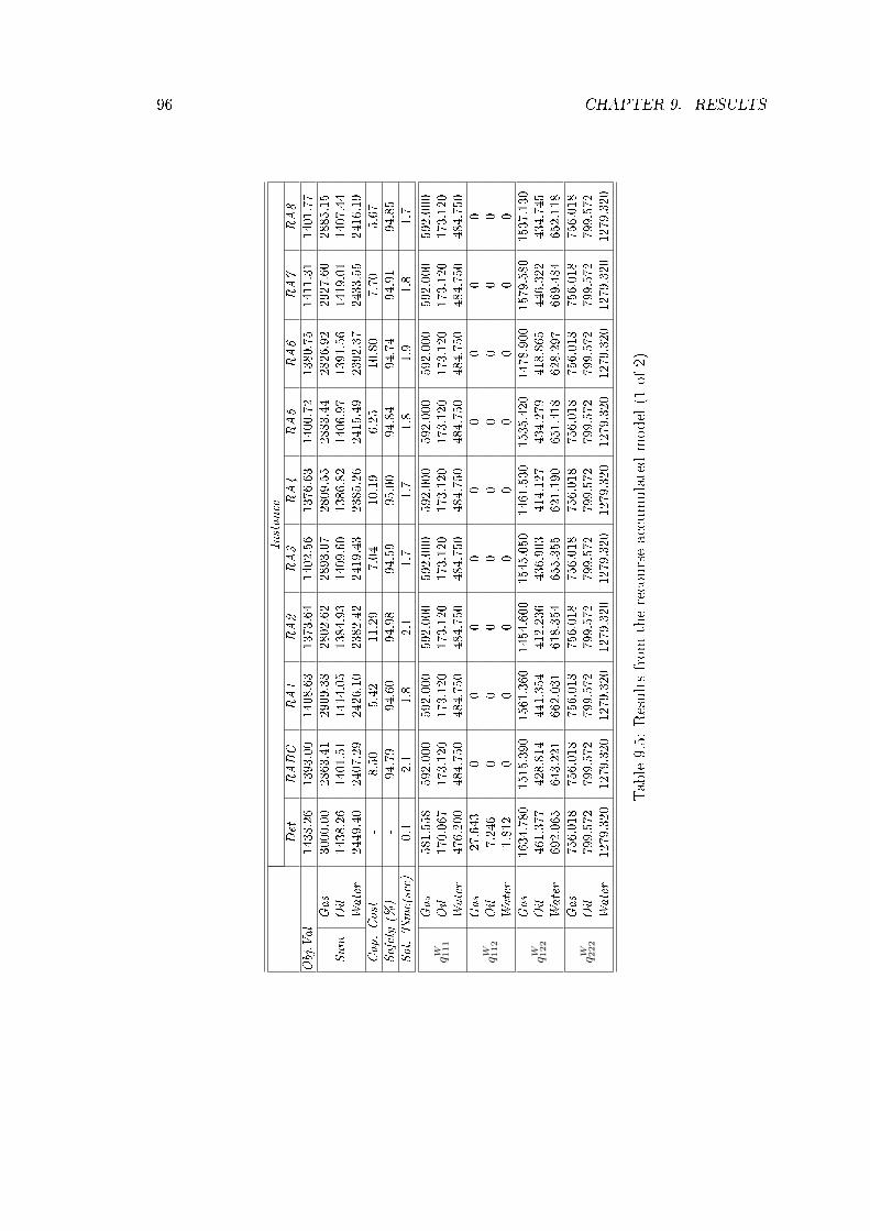
96 CHAPTER 9. RESULTS
Instance
Det
RABC
RA1
RA2
RA3
RA4
RA5
RA6
RA7
RA8
Obj.Val
1438.26
1393.00
1408.63
1373.64
1402.56
1376.63
1400.72
1380.75
1411.31
1401.77
Sum
Gas
3000.00
2863.41
2909.38
2802.62
2893.07
2809.55
2883.44
2826.92
2927.60
2885.15
Oil
1438.26
1401.51
1414.05
1384.93
1409.60
1386.82
1406.97
1391.56
1419.01
1407.44
Water
2449.40
2407.29
2426.10
2382.42
2419.43
2385.26
2415.49
2392.37
2433.55
2416.19
Cap.Cost
-8.50
5.42
11.29
7.04
10.19
6.25
10.80
7.70
5.67
Safety
(%)
-94.79
94.60
94.98
94.59
95.00
94.84
94.74
94.91
94.85
Sol.Tim
e(sec)
0.1
2.1
1.8
2.1
1.7
1.7
1.8
1.9
1.8
1.7
qW 111
Gas
581.558
592.000
592.000
592.000
592.000
592.000
592.000
592.000
592.000
592.000
Oil
170.067
173.120
173.120
173.120
173.120
173.120
173.120
173.120
173.120
173.120
Water
476.200
484.750
484.750
484.750
484.750
484.750
484.750
484.750
484.750
484.750
qW 112
Gas
27.643
00
00
00
00
0Oil
7.246
00
00
00
00
0Water
1.812
00
00
00
00
0
qW 122
Gas
1634.780
1515.390
1561.360
1454.600
1545.050
1461.530
1535.420
1478.900
1579.580
1537.130
Oil
461.377
428.814
441.354
412.236
436.903
414.127
434.279
418.865
446.322
434.745
Water
692.065
643.221
662.031
618.354
655.355
621.190
651.418
628.297
669.484
652.118
qW 222
Gas
756.018
756.018
756.018
756.018
756.018
756.018
756.018
756.018
756.018
756.018
Oil
799.572
799.572
799.572
799.572
799.572
799.572
799.572
799.572
799.572
799.572
Water
1279.320
1279.320
1279.320
1279.320
1279.320
1279.320
1279.320
1279.320
1279.320
1279.320
Table9.5:
Resultsfrom
therecourseaccumulatedmodel(1
of2)

9.3. VALUATION OF THE RECOURSE MODEL SOLUTIONS 97
Instance
RA9
RA10
RA11
RA12
Obj.Val
1410.12
1397.60
1390.27
1388.36
Sum
Gas
2945.17
2884.32
2850.80
2842.67
Oil
1423.81
1407.21
1398.07
1395.85
Water
2440.74
2415.85
2402.14
2398.81
Cap.Cost
13.69
9.61
7.80
7.49
Safety
(%)
73.50
91.28
96.29
97.11
Sol.Tim
e(sec)
1.8
2.3
1.7
1.6
qW 111
Gas
592.000
592.000
592.000
592.000
Oil
173.120
173.120
173.120
173.120
Water
484.750
484.750
484.750
484.750
qW 112
Gas
00
00
Oil
00
00
Water
00
00
qW 111
Gas
1597.150
1536.300
1502.780
1494.650
Oil
451.113
434.519
425.377
423.159
Water
676.670
651.778
638.066
634.739
qW 222
Gas
756.018
756.018
756.018
756.018
Oil
799.572
799.572
799.572
799.572
Water
1279.320
1279.320
1279.320
1279.320
Table9.6:
Resultsfrom
therecourseaccumulatedmodel(2
of2)
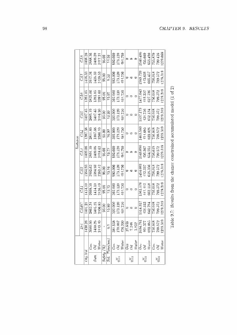
98 CHAPTER 9. RESULTS
Instance
Det
CABC
CA1
CA2
CA3
CA4
CA5
CA6
CA7
CA8
Obj.Val
1438.26
1401.21
1414.10
1384.93
1409.06
1387.38
1407.45
1391.05
1416.33
1408.20
Sum
Gas
3000.00
2862.34
2909.59
2802.62
2891.10
2811.60
2885.19
2825.06
2917.76
2888.36
Oil
1438.26
1401.21
1414.10
1384.93
1409.06
1387.38
1407.45
1391.05
1416.33
1408.20
Water
2449.40
2406.85
2426.19
2382.42
2418.62
2386.10
2416.20
2391.60
2429.53
2417.31
Safety
(%)
-95.00
95.00
95.00
95.00
95.00
95.00
95.00
95.00
95.00
Sol.Tim
e(sec)
0.1
15.89
13.25
13.16
13.72
16.92
13.39
15.97
8.53
14.50
qW 111
Gas
581.558
592.000
592.000
592.000
592.000
592.000
592.000
592.000
592.000
592.000
Oil
170.067
173.120
173.120
173.120
173.120
173.120
173.120
173.120
173.120
173.120
Water
476.200
484.750
484.750
484.750
484.750
484.750
484.750
484.750
484.750
484.750
qW 112
Gas
27.643
00
00
00
00
0Oil
7.246
00
00
00
00
0Water
1.812
00
00
00
00
0
qW 122
Gas
1634.781
1514.317
1561.576
1454.603
1543.080
1463.580
1537.173
1477.043
1569.739
1540.486
Oil
461.377
428.523
441.412
412.237
436.367
414.685
434.756
418.357
443.638
435.660
Water
692.065
642.784
662.118
618.356
654.551
622.028
652.134
627.536
665.457
653.490
qW 222
Gas
756.018
756.018
756.018
756.018
756.018
756.018
756.018
756.018
756.018
755.870
Oil
799.572
799.572
799.572
799.572
799.572
799.572
799.572
799.572
799.572
799.416
Water
1279.319
1279.319
1279.319
1279.319
1279.319
1279.319
1279.319
1279.319
1279.319
1279.069
Table9.7:
Resultsfrom
thechance
constrained
accumulatedmodel(1
of2)

9.3. VALUATION OF THE RECOURSE MODEL SOLUTIONS 99
Instance
CA9
CA10
CA11
CA12
Obj.Val
1409.27
1405.75
1394.33
1386.42
Sum
Gas
2891.87
2878.96
2837.07
2808.11
Oil
1409.27
1405.75
1394.33
1386.42
Water
2418.93
2413.65
2396.52
2384.67
Safety
(%)
90.00
92.50
97.50
99.00
Sol.Tim
e(sec)
17.45
16.66
14.80
17.19
qW 111
Gas
592.000
592.000
592.000
592.000
Oil
173.120
173.120
173.120
173.120
Water
484.750
484.750
484.750
484.750
qW 112
Gas
00
00
Oil
00
00
Water
00
00
qW 122
Gas
1543.851
1530.939
1489.056
1460.088
Oil
436.578
433.056
421.634
413.733
Water
654.866
649.584
632.450
620.599
qW 222
Gas
756.018
756.018
756.018
756.018
Oil
799.572
799.572
799.572
799.572
Water
1279.319
1279.319
1279.319
1279.319
Table9.8:
Resultsfrom
thechance
constrained
accumulatedmodel(2
of2)

100 CHAPTER 9. RESULTS
Instance
Det
RWBC
RW1
RW2
RW3
RW4
RW5
RW6
RW7
RW8
Obj.Val
1438.26
1382.56
1383.00
1378.18
1370.61
1370.35
1391.06
1373.72
1359.47
1357.62
Expected
Sum
Gas
3000.00
2877.32
2882.43
2870.77
2844.84
2873.34
2907.14
2871.37
2869.12
2881.05
Oil
1438.26
1395.06
1396.05
1392.08
1384.48
1383.71
1402.83
1387.71
1372.34
1371.29
Water
2449.40
2396.29
2398.11
2393.72
2349.35
2111.86
2408.83
2209.38
2014.26
1921.69
Cap.Cost
-7.10
8.17
8.59
8.10
8.21
6.22
8.39
7.75
8.35
Press.Cost
-5.40
4.89
5.31
5.76
5.14
5.55
5.60
5.12
5.32
Safety
(%)
-94.80
94.80
94.80
94.80
95.00
94.70
94.90
94.90
95.00
Sol.Tim
e(sec)
0.1
38.6
38.1
40.9
38.8
40.1
39.4
38.9
36.0
40.3
γ111
k
10
00
00
00
00
02
00
00
00
00
00
30
00
00
00
00
04
0.9824
11
10.8525
0.2279
11
11
50.0176
00
00.1475
0.7721
00
00
γ112
k
10
00
00
00
00
02
00
00
00
00
00
30
00
00
00
00
04
0.0154
00
00
0.1536
00.3020
0.5909
0.7439
50.9846
11
11
0.8464
10.6980
0.4091
0.2561
γ122
k
10
00
00
00
00
02
00
00
00
00
00
30.8837
0.7567
0.7602
0.7471
0.8335
10.7959
00
04
0.1163
0.2433
0.2398
0.2529
0.1665
00.2041
10.4758
0.2124
50
00
00
00
00.5242
0.7876
γ222
k
10
00
00
00
00
02
00
00
00
00
00
30
00
00
00
00
04
0.8711
0.8565
0.8562
0.8557
0.8562
0.8566
0.8555
0.8572
0.8566
0.8570
50.1289
0.1435
0.1438
0.1443
0.1438
0.1434
0.1445
0.1428
0.1434
0.1430
Table9.9:
Resultsfrom
therecoursewellmodel(1
of2)

9.3. VALUATION OF THE RECOURSE MODEL SOLUTIONS 101
Instance
RW9
RW10
RW11
RW12
RW13
RW14
RW15
Obj.Val
1396.83
1369.64
1338.52
1291.94
1410.41
1394.50
1383.12
Expected
Sum
Gas
2889.10
2863.58
2841.90
2793.15
2922.07
2912.33
2896.51
Oil
1405.88
1386.24
1363.52
1325.67
1417.51
1404.87
1395.78
Water
2412.94
2377.20
2337.43
2291.59
2431.29
2413.42
2257.99
Cap.Cost
7.23
8.19
9.57
14.96
7.10
5.01
8.07
Press.Cost
1.82
8.41
15.42
18.77
05.36
4.59
Safety
(%)
94.80
94.80
94.70
94.70
94.60
94.90
94.90
Sol.Tim
e(sec)
44.0
38.5
35.4
62.3
4.4
38.7
29.8
γ111
k
10
00
00
00
20
00
00
00
30
00
00
00
41
11
11
11
50
00
00
00
γ112
k
10
00
00
00
20
00
00
00
30
00
00
00
40
00
00
00.2389
51
11
11
10.7611
γ122
k
10
00
00
00
20
00
00
00
30.7614
0.7482
0.7513
0.7147
0.8001
0.8034
0.1914
40.2386
0.2518
0.2487
0.2853
0.1999
0.1966
0.8086
50
00
00
00
γ222
k
10
00
00
00
20
00
00
00
30
00
00
00
40.8663
0.8473
0.8194
0.7915
0.8711
0.8565
0.8557
50.1337
0.1527
0.1806
0.2085
0.1289
0.1435
0.1443
Table9.10:Resultsfrom
therecoursewellmodel(2
of2)

102 CHAPTER 9. RESULTS

Chapter 10
Discussion
In this chapter, the results reported in the previous chapter are further discussed. Section10.1 evaluates the e�ects of uncertainties on the solutions obtained from the stochasticmodels, and the safety level and recourse costs are addressed. The advantages of applyingstochastic models are discussed in Section 10.2, and additional remarks are summarizedin Section 10.3.
10.1 E�ects of the Stochastic Model Parameters
The two main elements a�ecting the results obtained from the stochastic models arethe standard deviations of the uncertain parameters and the unit recourse cost or safetylevel. The e�ects of varying these parameters are discussed in the following.
10.1.1 E�ects of Uncertainty
The results presented in the previous chapter illustrate a strong relation between the un-certainty level of the Troll C production system, and the objective value of the stochasticmodels. When uncertainty is increased, the production is lowered. The same observa-tions apply to both approaches of incorporating the uncertainties of the �ow estimates.Disregarding whether it is modeled at an accumulated level or at well level, uncertaintyreduces the objective value of the stochastic models.
In the chance constrained accumulated model, the reduced production is a result of alarger barrier term, preventing the gas capacity constraint from being violated. As thestandard deviations of the uncertain parameters are increased, the size of the barrier termgrows, implying the gas production is increasingly restricted. As the �ow of all phases iscorrelated, this leads to a reduced oil production, and thus lower objective value.
103
104 CHAPTER 10. DISCUSSION
When the standard deviation of the uncertain parameters grows, the possible deviationsbetween the estimated and the true �ow increase. In the recourse models, larger �owvariations imply a need for increased compensations from the recourse variables, to avoidconstraint violations. Both the frequency and the size of the required compensationsdecrease when the production is lowered. Production is thus reduced to avoid high totalrecourse costs.
The results presented in the previous chapter illustrate shifts in the production rateswhen uncertainties are unevenly distributed among the clusters or wells. Productionis transferred from uncertain to less uncertain parts of the system. For the chance con-strained model, the reasons for these shifts can be explained by studying the probabilisticgas capacity constraint:
∑i∈I
AiqPimp + Φ−1(η)
√∑i∈I
(σAi q
Pimp
)2+ (σK)2 ≤ K , m = {1}, p = {g}, (10.1)
The terms σAi qPimp increase when the uncertainty level grows. To compensate for an
increase in the standard deviations σAi , the production qPimp must be reduced, and possibly
transferred to other clusters where the uncertainty level is lower.
In the recourse models, the chance of high recourse costs increases when the uncertaintylevel grows. To avoid this, when the uncertainty of the system is evenly distributed,the only alternative is to reduce the total production. If a cluster or well has a higheruncertainty level compared to the other parts of the system, production can be transferredto the less uncertain wells or clusters. The variation in the total �ow will thus decrease,and accordingly the total expected recourse costs are reduced.
By studying the instances RW5 to RW8 of the recourse well model, the e�ects of pro-duction shifts are evident. When the uncertainty levels of the �ow predictions for well122 increase, production is transferred to other less uncertain wells. As the total levelof uncertainty in the system is increased, the objective value is reduced.
The tendency of prioritizing the least uncertain wells or clusters is inevitably pro�tablein the short run. However, if all the wells will eventually be fully recovered, the gainsare more ambiguous. When producing from a well, new production data may improvethe estimates for the future production rates, which is a good argument for producingfrom the wells that are uncertain today. Nevertheless, uncertainties may be revealed overtime, as new technology can improve the production estimates in the future, encouragingdelayed production from uncertain wells and clusters.
Shifts in production can be observed in all the instances of the well model testing thee�ects of di�erent uncertainty levels for the various wells. However, the impact is not ofthe same magnitude for all the wells. Consider the instances RW9 to RW12 of Table 9.10

10.1. EFFECTS OF THE STOCHASTIC MODEL PARAMETERS 105
in the previous chapter, where the uncertainty level of well 222 is varied. The gas/oil-ratio (GOR) of this well is low, which can be concluded from studying Figure 9.1. Alarge amount of oil can thus be produced without consuming too much of the availablegas capacity at the platform, which suggests 222 is a pro�table well. High total recoursecosts are thus accepted to maintain production from this well. It is clear that the shifts inproduction from well 222 are less signi�cant compared to well 122 in instances RW5 toRW8, implying changes in the uncertainty levels have less impact on the most pro�tablewells.
10.1.2 E�ects of Safety Level and Recourse Costs
The safety level of the chance constrained model controls the probability of not exceedingthe gas capacity constraint. From Table 9.8 in the previous chapter, it is evident thatthe objective value decreases when the safety level is increased. Again, this is a result ofa larger barrier term, enforcing a lower production. Figure 10.1 illustrates the relationbetween objective value and safety level of the chance constrained accumulated model.The marginal change of the objective is increasing as the safety level grows.
Safety Obj.Val90 % 1409
92.50 % 140695 % 1401
97.50 % 139499 % 1386
99.90 % 137099.90 % 1370
1400
1410
1420
Val
ue
1370
1380
1390
1400
1410
1420
90 % 92 % 94 % 96 % 98 % 100 %
Obj
ectiv
e V
alue
1370
1380
1390
1400
1410
1420
90 % 92 % 94 % 96 % 98 % 100 %
Obj
ectiv
e V
alue
Safety Level
Sigma (%) Obj.val1 14143 14013 14015 13857 13689 1352
11 133715 130820 1275
Figure 10.1: Relation between objective value and safety level for the chance constrainedaccumulated model
When the safety level approaches 100%, there is a substantial reduction in the objectivevalue. There is always a chance that an extreme outcome for one of the uncertainparameters will lead to constraint violations. It is theoretically impossible to reach asafety level of 100%, because of the in�nitely long tails of the normal distribution.
In the recourse models, the recourse costs penalize compensations for constraint viola-tions through the recourse variables. When the recourse costs are increased, the objectivevalue is lowered, as illustrated by the instances RA9 to RA12 of Table 9.6 in the previ-ous chapter. It is pro�table to reduce production to avoid recourse costs. Figure 10.2illustrates the �ndings.

106 CHAPTER 10. DISCUSSION
1370
1380
1390
1400
1410
1420
0 5 10 15 20 25 30 35
Obj
ectiv
e Val
ue
Recourse Cost
Figure 10.2: Relation between objective value and recourse costs for the recourse accu-mulated model
High recourse costs give rise to solutions where compensations to a large extent areavoided. This implies the recourse variables are close to zero, and the e�ects of furtherincreasing the recourse unit costs are less signi�cant, see Figure 10.2. Accordingly, theobjective value is a�ected to a lower extent when the costs are high in the �rst place.This is in line with the total recourse costs reported for RA9 to RA12 in Table 9.6, whichdecrease when the unit recourse costs are increased.
The safety level obtained by the recourse models increases when the unit recourse costsare increased, which is illustrated in Figure 10.3. As for the chance constrained model,it is di�cult to obtain a safety level approaching 100%. To accomplish this, a recoursecost approaching in�nity is required.
Safety Cost74 % 187 % 291 % 393 % 495 % 596 % 696 % 797 % 897 % 997 % 1098 % 1599 % 2099 % 30
05
101520253035
70 % 75 % 80 % 85 % 90 % 95 % 100 %
Rec
ours
e C
ost
Safety Level
Cost Obj.Val1 14102 14023 13984 13955 13936 13927 13908 13899 1388
10 138815 138520 138330 1380
05
101520253035
70 % 75 % 80 % 85 % 90 % 95 % 100 %
Rec
ours
e C
ost
Safety Level
1400
1410
1420
ve V
alue
Figure 10.3: Relation between safety level and recourse costs for the recourse accumulatedmodel

10.2. EVALUATION OF MODELS 107
When comparing the recourse and chance constrained models, similar consequences ofuncertainties are observed. The main di�erences between the recourse and chance con-strained accumulated models are the mechanisms for avoiding constraint violations. Inthe chance constrained model, the safety level speci�es the desired probability of notexceeding the capacity constraint. The chance constrained problem is underdetermined,implying it is not possible to calculate the optimal probability level. The optimal solutionto the problem can only be given for a pre-speci�ed safety level, and the decision makeris left with a trade-o� between safety and pro�tability. In many practical problems, thereare external requirements for the safety level of a system, due to for example contractualagreements or company policies. This implies a suitable safety level is given.
In the recourse model, an appropriate recourse cost must be determined to ensure thatcompensations for constraint violations are penalized su�ciently. For a given cost ofconstraint violations, the optimal safety level can be calculated from the solution of therecourse model. It is a challenge to evaluate the e�ects of exceeding the gas capacitylimit in terms of the objective, which is given by the total oil production. In the modelsdeveloped in this thesis, the recourse cost is obtained through testing, where the resultingsafety level is considered important. Emphasizing the safety level obtained from a speci�crecourse cost, gives rise to the same challenges as when determining the safety level of achance constrained model.
There is a strong relation between the recourse cost and safety level. If the correctcost of constraint violations can be assessed, the corresponding optimal safety level canbe determined, and vice versa. In this thesis, the safety level forms the basis for theparameter settings, as the the cost of exceeding the capacity constraint is di�cult toobtain. It is assumed that an appropriate safety level can be determined, due to reliabilityrequirements at the platform.
10.2 Evaluation of Models
From the results presented in the previous chapter, it is clear that deterministic objectivevalue is superior to the stochastic solutions. However, the deterministic model does notaccount for uncertainties, and constraint violations are likely to occur as a result ofdeviating model parameters. In an uncertain environment, the deterministic solutionwill no longer be optimal.
The uncertain parameters of the stochastic models are assumed to be normally dis-tributed. If this had been an exact representation of the real production system, im-plementing the deterministic solution would result in constraint violations in 50% of thetime. In the chance constrained model, a safety level of 50% eliminates the barrier term,as Φ−1(0.5) = 0, and the resulting problem is deterministic. The deterministic solutionis thus the same as a chance constrained solution with a low safety level.
As discussed in Chapter 3, it is not possible to evaluate the solutions obtained from a

108 CHAPTER 10. DISCUSSION
chance constrained model quantitatively. In order to obtain a measure for the value ofapplying stochastic problem formulations, the recourse models must be studied. Thevalue of the stochastic solution (VSS) is presented in Table 9.2 in the previous chapter.It is obvious that the expected value solutions1 perform poorly when implemented in anuncertain environment. The objective value is low, as compensation is needed to avoidconstraint violations. Again, the safety level of applying a deterministic or EV solutionis close to 50%, analogous to the �ndings from the chance constrained model.
The values of the stochastic solutions presented in the previous chapter are signi�cant.Applying recourse models as an alternative to the deterministic model will increase thepro�tability by more than 10% for both the recourse well and the recourse accumulatedmodels. These results indicate it is worth the e�ort to develop and solve stochasticmodels for the production planning problem at Troll C.
The possibility to quantitatively evaluate the stochastic solution is one of the majoradvantages of the recourse models. Without the VSS, it is di�cult to assess the bene�tsfrom developing a stochastic model for the production planning problem.
Some of the uncertainties arising in optimization models can be reduced by studying thesources of uncertainties more thoroughly. In the production planning problem presentedin this thesis, uncertainties related to the �ow predictions and the capacity limit aretreated. Possibly, the uncertainties related to the �ow predictions may be reduced byinvesting in more advanced technology, and better forecasting techniques could haveimproved the predictions of the gas capacity limit. It is di�cult to determine which ofthese e�orts are the most pro�table. In theory, it is possible to eliminate the internaluncertainties arising from modeling of the �ow. The variations in the capacity limit aredetermined by external factors, which cannot be controlled. Nevertheless, the variationscan be described more accurately. Results presented in the previous chapter indicate thatreducing the uncertainty of the �ow predictions improve the objective value the most,which is expected as the uncertainty level is higher for the �ow estimates than for thecapacity limit. However, the costs of uncertainty reductions should also be considered.
The expected value of perfect information (EVPI) is a measure of the possible gainsfrom eliminating all the uncertainties arising in the production optimization problem.The EVPIs for the planning problems at Troll C are given in Table 9.4, and indicatethat the potential from totally removing the uncertainties is smaller than the gains fromapplying a stochastic model. The objective value can only be improved by 3%, whichshould be taken into account when considering alternatives for reducing uncertainty. Ifthe costs of obtaining better �ow estimates or gas capacity forecasts are higher than theEVPI, it is not pro�table to implement the improvements.
1The EV in the recourse well model is assumed to be representative for the deterministic solution.

10.3. PRACTICAL CONSIDERATIONS 109
10.3 Practical Considerations
The models presented in this thesis are simpli�ed representations of the real productionsystem at Troll C. The problem considered is small compared to the total structure;only two out of eight clusters are incorporated in the models. In reality, there are two�ow lines from each manifold, whereas one is included in this thesis. Furthermore, toreduce the complexity of the models, the nonlinear pressure drop curves are representedby linear functions. These simpli�cations limit the practical use of the models.
The stochastic models assume normally distributed parameters, which is probably not thetrue distribution of these coe�cients. It is not possible to incorporate all eventualitiesin a stochastic model, thus the solutions obtained are not optimal in the real world.However, it is better to base decisions on the assumption that the parameters can takeon di�erent values, compared to one �xed value, as in a deterministic model (Wets, 1996).

110 CHAPTER 10. DISCUSSION

Chapter 11
Conclusion
Optimizing petroleum production at the Troll C platform is a challenging task, where�ow predictions are crucial in order to model the production system. Predicting themultiphase wellstreams is involved, due to the thin oil layer in the reservoir. Furthercomplicating the problem is the varying gas capacity limit at the platform. These factorsbring uncertainty into an optimization model for the production planning problem atTroll C.
A deterministic model fails to account for the uncertainties related to the production op-timization problem. Implementing a deterministic solution in the uncertain environmentmay lead to constraint violations and suboptimal solutions. In the planning problemat Troll C, the gas capacity constraint can be violated, as it is exposed to variations inthe predicted gas �ow and capacity limit. Stochastic models should thus be developed,incorporating these uncertainties.
In this thesis, both chance constrained and recourse models are applied to the productionoptimization problem, treating uncertain �ow predictions and capacity limit. Despite thedi�erent structure of the formulations, the models provide practically equivalent resultswhen tested on identical instances, and there is a close link between the recourse cost ofthe recourse formulations and the probability level of the chance constrained formulation.
Specifying the recourse cost is troublesome, as measuring the consequences of exceedingthe capacity constraint in terms of the objective value is di�cult. It is less complicatedto specify a probability level, as needed for the chance constrained model. However, aprobability level can be calculated for the recourse models as the percentage of time thecapacity constraint is satis�ed without compensation from the recourse variables. Therecourse cost can thus be set in accordance with a desired probability level.
The models proposed in this thesis represent alternative approaches for incorporatinguncertainty related to the �ow. The aggregated uncertainties, arising from the total�ow estimates for a cluster of wells, are considered in the accumulated models, while thewell model treats well-speci�c uncertainties resulting from the �ow predictions of the
111

112 CHAPTER 11. CONCLUSION
separate wells. Only the recourse method proves to be applicable at well level, whereasboth chance constrained and recourse models are appropriate at the accumulated level.
When the uncertainty level grows, the objective value obtained from the stochastic modelsis lowered, and production is shifted from uncertain to less uncertain parts of the system.Production is also reduced as the safety level or recourse costs are increased. These resultsapply to all the proposed models.
The recourse models allow for a quantitative assessment of the gains from implementing astochastic solution. Evaluating the recourse models for the production planning problemat Troll C, it is obvious that the solutions obtained are superior to the deterministic orexpected value solutions exposed to uncertainties. The objective value is increased bymore than 10% when implementing the stochastic solutions. This proves that the gainsfrom developing and solving the recourse models are substantial.
Comparing the models treating uncertainty at an accumulated level and at well level, itis clear that the well model provides valuable additional information. Although similare�ects from uncertainty are observed, the recourse well model incorporates more detailsregarding the uncertainties of the production system, and thus o�ers solutions accountingfor well-speci�c information. This insight is not obtained from the accumulated mod-els, thus the recourse well model is considered the most appropriate for the productionplanning problem.
The models presented in this thesis are simpli�ed representations of the real productionsystem at Troll C. Further research should be conducted to assess more accurate repre-sentations of the uncertainties related to the production system, and the models shouldbe re�ned in order to implement the solutions in practice. However, the results providedindicate signi�cant potentials from applying stochastic models to the planning problem,encouraging further studies.

Chapter 12
Further Work
The models proposed in this thesis are subject to several assumptions and simpli�cations.The main purpose is to study the e�ects of uncertainty in a mathematical model, andto compare alternative approaches of incorporating uncertainty in stochastic models.Further development and re�nements are recommended in order to apply the models tothe real planning problem at Troll C.
The deterministic model, which serves as the basis for the stochastic models in this thesis,is simpli�ed to ensure computational tractability of the corresponding chance constrainedand recourse models. The real production system at Troll C consists of two pipelinesfrom each manifold, which allows for production from both high and low pressure wellssimultaneously. Some of the wells at the Troll C �eld have gas lift risers, which enhancethe recovery. These system properties are not incorporated in the models presented, andshould be included in a more realistic model.
The pressure drop curves describing the pressure drop through the pipelines from themanifolds to the platform are highly simpli�ed, represented by linear functions. In reality,these are nonlinear relations, and should at least be modeled as piecewise linear functionsas the WPCs. This will increase the complexity of the model signi�cantly. Moreover,the pressure drop is modeled to be independent of the absolute pressure, which is notthe case in reality.
Representing the WPCs by �ve breakpoints is considered to be su�cient for the problemssolved in this thesis. However, the number can be increased to improve the accuracy of theresults. Additionally, the underlying nonlinear functions are approximations of the realWPC relations. The piecewise linear representation allows for applying real productionsimulation data, however, this requires higher resolution, obtained by introducing morebreakpoints.
Varying gas capacity limit and �ow estimates are the sole sources of uncertainty consid-ered in this thesis. Other parts of the production system may also be treated as uncertain,
113

114 CHAPTER 12. FURTHER WORK
for example the pressure drop curves, which are di�cult to express mathematically. Thiswould provide a more complete model of the situation at Troll C.
In the recourse models, the recourse costs for the gas capacity surplus variables are set inorder to obtain an appropriate safety level, as the reliability of the system is consideredimportant. The consequences of violating the gas capacity constraint should be furtherstudied in order to give a realistic estimate for the true costs of violations. If it is possibleto de�ne these costs, the safety level need not be considered when solving the model, butcan be calculated from the solutions obtained.
The uncertain parameters of the proposed models are assumed to be normally distributed,as no speci�c information of the distributions are available today. Further investigationsshould be conducted to obtain more accurate information regarding the possible out-comes of the uncertain coe�cients. Other distribution functions can be considered forthe recourse models, as long as discretization or sampling is possible. For the chanceconstrained formulation, the alternative distributions are limited when convexity of themodel is a requirement. Closer cooperation with StatoilHydro is needed in order toobtain a better picture of the uncertainty at the �eld.
The suggested improvements will increase the size and complexity of the models proposed,which results in less tractable formulations. This is a challenge, particularly for therecourse models, where the uncertainties are represented by a large number of scenarios.If more uncertainties are introduced, the number of scenarios must be further increasedto provide the same accuracy of the representation. Although the SAA method reducesthe problem size, other solution methods, such as decomposition, might be necessary inorder to solve the problems.

Bibliography
Al-Othman, W. B., Lababidi, H. M., Alatiqi, I. M. and Al-Shayji, K. (2007), `Supplychain optimization of petroleum organization under uncertainty in market demandsand prices', European Journal of Operational Research 189, 822�840.
Arellano-Garcia, H. (2006), Chance Constrained Optimization of Process Systems underUncertainty, PhD thesis, Technischen Universität Berlin.
Ashford, R. (2007), `Mixed integer programming: A historical perspective with Xpress-MP', Annals of Operations Research 145, 5�17.
Ben-Tal, A. and Nemirovski, A. (1998), `Robust convex optimization', Mathematics ofOperations Research 23, 769�805.
Bieker, H. P., Slupphaug, O. and Johansen, T. A. (2006a), Global Optimization of Multi-phase Flow Networks in Oil and Gas Production Systems, in `Computers & ChemicalEngineering Journal, presented at 2006 AIChE Annual Meeting', San Fransisco, Cali-fornia, USA.
Bieker, H. P., Slupphaug, O. and Johansen, T. A. (2006b), Optimal well-testing strategyfor production optimization: A monte carlo simulation approach, in `SPE EasternRegional Meeting', Canton, Ohio, SPE 104535.
Bieker, H. P., Slupphaug, O. and Johansen, T. A. (2007a), `Real�time production op-timization of o�shore oil and gas production systems: A technology survey', SPEProduction and Operations 22(4), 382�391. SPE 99446.
Bieker, H. P., Slupphaug, O. and Johansen, T. A. (2007b), Well Management underUncertain Gas or Water Oil ratios, in `SPE Digital Energy Conference and Exhibtion',Houston, Texas. SPE 106959.
Birge, J. R. (1997), `Stochastic Programming Computation and Applications:', IN-FORMS Journal on Computing 9(2), 111�133.
Birge, J. R. and Louveaux, F. (1997), Introduction to Stochastic Programming, SpringerSeries in Operations Research.
115

116 BIBLIOGRAPHY
Blau, R. A. (1974), `Stochastic Programming and Decision Analysis: An ApparentDilemma', Management Science 21(3), 271�276.
Bonami, P. and Lee, J. (2007), BONMIN Users' Manual, COIN-OR. Downloaded Jan-uary 8, 2009.URL: http://www.coin-or.org/Bonmin/index.html
Boyd, S. P. and Vandenberghe, L. (2003), Convex Optimization, Cambridge UniversityPress. Material available at:.URL: http://www.stanford.edu/-boyd
Carøe, C. C. and Schultz, R. (1999), `Dual decomposition in stochastic integer program-ming', Operations Research Letters 24, 37�45.
Charnes, A. and Cooper, W. (1959), `Chance-Constrained Programming', ManagementScience 6(1), 73�79.
Charnes, A. and Cooper, W. (1983), `Response to "Decision Problems under Risk andChance Constrained Programming: Dilemmas in the Transition"', Management Sci-ence 29(6), 750�753.
Charnes, A., Cooper, W. W. and Symonds, G. H. (1958), `Cost Horizons and CertaintyEquivalents: An Approach to Stochastic Programming of Heating Oil', ManagementScience 4(3), 235�263.
COIN-OR (2009), `COIN-OR homepage'. Accessed March 14, 2009.URL: http:// www.coin-or.org
Czyzyk, J., Mesnier, M. P. and Moré, J. J. (1998), `The NEOS server', IEEE Computa-tional Science & Engineering 5(3), 68�75.
Dantzig, G. B. (1955), `Linear Programming under Uncertainty', Management Science1(3/4), 197�206.
Dash Optimization (2007), Xpress-MP Getting Started, Dash Optimization Ltd. Down-loaded May 7, 2009.URL: http://www.artelys.com/fr/composants/xpress-mp-documentation.html
Dueñas Díez, M. (2007), `How to optimize a petroleum �eld with 54 wells? What can bedone and what cannot', Presented at the IO Conference 2007.
Dueñas Díez, M., Brusdal, K., Evensen, G., Barkve, T. and Mjaavatten, A. (2006), Op-portunities and challenges of using sequential quadratic programming (SQP) for op-timization of petroleum production networks, in `European Symposium on ComputerAided Process Engineering - 15'.
Elgsaeter, S. M. (2008), Modeling and Optimizing the O�shore Production of Oil andGas under Uncertainty, PhD thesis, Norwegian University of Science and Technology,Trondheim, Norway.

BIBLIOGRAPHY 117
Foss, B., Gunnerud, V. and Dueñas Díez, M. (2009), Lagrangian decomposition of oilproduction optimization - applied to the Troll west oil rim. Accepted for the SPEJournal. SPE 118299.
GAMS Home Page (2009). Accessed January 17,2009.URL: http://www.gams.com
Garstka, S. J. and Wets, R. J.-B. (1974), `Decision Rules in Stochastic Programming',Mathematical Programming 7, 117�143.
Glæserud, P. and Syrdalen, J. A. (2008), `Production Optimization under Uncertainty- Applied to the Troll C Field', Project thesis, Norwegian University of Science andTechnology, Trondheim, Norway.
Goel, V. and Grossmann, I. E. (2004), `A stochastic programming approach to planning ofo�shore gas �eld developments under uncertainty in reserves', Computers and ChemicalEngineering 28, 1409�1429.
Gunnerud, V., Foss, B., Nygren, B., Vestbø, R. and Walberg, N. C. (2009), Dantzig-Wolfe decomposition for real-time optimization - applied to the Troll west oil rim, in`ADCHEM 2009', Istanbul, Turkey.
Gunnerud, V. and Langvik, E. (2007), Production Planning Optimization for the TrollC Field, Master's thesis, Norwegian University of Science and Technology, Trondheim,Norway.
Guéret, C., Prins, C. and Sevaux, M. (2007), Applications of optimization with Xpress-MP, Dash Optimization Ltd. Downloaded May 7, 2009.URL: http://www.dashoptimization.com
Hauge, J. and Horn, T. (2005), The challenge of operating and maintaining 115 subseawells on the Troll �eld, in `O�shore Technology Conference', Houston, TX, USA. OTC17111.
Haugen, K. K. (1996), `A Stochastic Dynamic Programming model for scheduling ofo�shore petroleum �elds with resource uncertainty', European Journal of OperationalResearch 88, 88�100.
Henrion, R. (2004), Introduction to Chance Constrained Programming, in `Tutorial paperfor the Stochastic Community Home Page', pp. 1�17. Downloaded January 16, 2009.URL: http://stoprog.org/
Henrion, R. and Strugarek, C. (2006), `Convexity of chance constraints with independentrandom variables', Computational Optimization and Applications 41, 263�276.
Higle, J. L. (2005), Stochastic Programming: Optimization When Uncertainty Matters,in `Tutorials in Operations Research Informs 2005'.

118 BIBLIOGRAPHY
Higle, J. L. and Sen, S. (1991), `Stochastic Decomposition: An Algorithm for Two-Stage Stochastic Linear Programs with Rrecourse', Mathematics of Operations Re-search 16(3), 650�669.
Hindi, H. (2004), A Tutorial on Convex Optimization, in `Proceeding of the 2004 Amer-ican Control Conference', Boston, Massachusetts.
Hogan, A. J., Morris, J. and Thompson, H. (1981), `Decision Problems under Risk andChance Constrained Programming: Dilemmas in the Transition', Management Science27(6), 698�716.
Hogan, A. J., Morris, J. and Thompson, H. (1984), `Reply to Professors Charnesand Cooper Concerning Their Response to "Decision Problems under Risk andChance Constrained Programming: Dilemmas in the Transition"', Management Sci-ence 30(2), 258�259.
Jonsbråten, T. W. (1998), `Oil �eld optimization under price uncertainty', Journal of theOperational Research Society 49, 811�818.
Jørnsten, K. O. (1992), `Sequencing o�shore oil and gas �elds under uncertainty', Euro-pean Journal of Operational Research 58, 191�201.
Kall, P. (1976), Stochastic Linear Programming, Springer-Verlag Berlin Heidelberg NewYork.
Kall, P. and Mayer, J. (2005), Stochastic Linear Programming � Models, Theory, andComputation, Springer's International Series in Operations Research & ManagementScience.
Kall, P. and Wallace, S. W. (1994), Stochastic Programming, Wiley�Interscience Seriesin Systems and Optimization.
Khor, C. S., Elkamel, A., Ponnambalam, K. and Douglas, P. L. (2008), `Two-stagestochastic programming with �xed recourse via scenario planning with economicand operational risk management for petroleum re�nery planning under uncertainty',Chemical Engineering and Processing 47, 1744�1764.
Klein Haneveld, W. K., Stougie, L. and van der Vlerk, M. H. (1996), `An algorithm forthe construction of convex hulls in simple integer recourse programming', Annals ofOperations Research 64, 67�81.
Klein Haneveld, W. K. and van der Vlerk, M. H. (2006), `Integrated chance constraints:reduced form and an algorithm', Computational Management Science 3(4), 245�269.
Kleywegt, A. J., Shapiro, A. and de Mello, T. H. (2001), `The Sample Average Approxi-mation Method for Stochastic Discrete Optimization', SIAM Journal of Optimization12(2), 479�502.

BIBLIOGRAPHY 119
Kosmidis, V. D., Perkins, J. D. and Pistikopoulos, E. N. (2005), `A Mixed integer opti-mization formulation for the well scheduling problem on petroleum �elds', Computersand Chemical Engineering 29, 1523�1541.
Löfberg, J. (2004), Yalmip : A toolbox for modeling and optimization in MATLAB, in`Proceedings of the CACSD Conference', Taipei, Taiwan.URL: http://control.ee.ethz.ch/ joloef/yalmip.php
Lougee-Heimer, R. (2003), `The Common Optimization INterface for Operations Re-search: Promoting open-source software in the operations research community', IBMJournal of Research & Development 42(1), 57�66.
Mak, W.-K., Morton, D. P. and Wood, R. K. (1999), `Monte Carlo bounding teqniquesfor determining solution quality in stochastic programs', Operations Research Letters24, 47�56.
Mally's Homepage (2009), `Homepage by Maarten H. van der Vlerk'. Accessed February28, 2009.URL: http://mally.eco.rug.nl/
McCarl, B. A. (2008), McCarl GAMS User Guide Version 22.9. Downloaded February10, 2009.URL: http://www.gams.com/docs/document.htm
Mjaavatten, A., Aasheim, R., Saelid, S. and Gronning, O. (2006), A Model for Gas Con-ing and Rate-Dependent Gas/Oil Ratio in an Oil-Rim Reservoir, in `The 2006 RussianOil and Gas Technical Conference and Exhibtion', Moscow, Russia. SPE 102390.
NEOS server (2009), `Homepage'. Accessed January 9, 2009.URL: http://neos.mcs.anl.gov/
Neumaier, A., Shcherbina, O., Huyer, W. and Tamás, V. (2005), `A comparison of com-plete global optimization solvers', Mathematical Programming 103, 335�356.
Nocedal, J. and Wright, S. J. (2006), Numerical Optimization, Springer Series in Opera-tions Research.
Norwegian Petroleum Directorate (2009), `Homepage'. Accessed January 24, 2009.URL: http://www.npd.no
Nygreen, B., Christiansen, M., Haugen, K., Bjørkvoll, T. and Kristiansen, O. (1998),`Modeling Norwegian petroleum production and transportation', Annals of OperationsResearch 82, 251�267.
Prékopa, A. (1970), On Probabilistic Constrained Programming, in `Proceedings of thePrinceton Symposium on Mathematical Programming', pp. 113�138.
Prékopa, A. (1973), `Contributions to the Theory of Stochastic Programming', Mathe-matical Programming 4, 202�221.
120 BIBLIOGRAPHY
Prékopa, A. (1995), Stochastic Programming, Kluwer Academic Publishers.
Rardin, R. L. (1998), Optimization in Operations Research, Prentice Hall Inc.
Rockafellar, R. and Wets, R. J.-B. (1991), `Scenarios and Policy Aggregation in Opti-mization under Uncertainty', Mathematics of Operations Research 16, 119�147.
Sahinidis, N. and Tawarmalani, M. (2005), BARON 7.2.5: Global Optimization of Mixed-Integer Nonlinear Programs, User's Manual. Downloaded January 9, 2009.URL: http://www.gams.com/dd/docs/solvers/baron.pdf
Schiozer, D. J., Ligero, E. L. and Santos, J. A. M. (2004), `Risk Assessment for Reser-voir Development Under Uncertainty', J. of the Braz. Soc. of Mech. Sci. & Eng.XXVI(2), 213�217.
Schütz, P., Tomasgard, A. and Shabbir, A. (2009), `Supply Chain Design under Un-certainty using Sample Average Approximation and Dual Decomposition', EuropeanJournal of Operational Research 199, 409�419.
Sen, S. and Higle, J. (1999), `An Introductory Tutorial on Stochastic Linear ProgrammingModels', Interfaces 29(2), 33�61.
Shapiro, A. (2001), Monte Carlo Simulation Approach to Stochastic Programming, in`Proceedings of the 2001 Winter Simulation Conference'.
Shapiro, A. and Philpott, A. (2007), `A tutorial on Stochastic Programming'. Down-loaded October 15, 2008.URL: http://www.stoprog.org/
StatoilHydro (2009), `Homepage'. Accessed May 28, 2009.URL: http://www.statoilhydro.com
Stochastic Programming Community Home Page (2009), `Homepage'. Accessed March6, 2009.URL: http://stoprog.org
Suslick, S. B. and Schiozer, D. J. (2004), `Risk Analysis Applied to Petroleum Explorationand Production: An Overview', Journal of Petroleum Science and Engineering 44, 1�9.
The Mathworks (2009), `Homepage MATLAB'. Accessed January 19, 2009.URL: www.mathworks.com
Ulstein, N. L., Nygreen, B. and Sagli, J. R. (2007), `Tactical planning of o�shorepetroleum production', European Journal of Operations Research 176, 550�564.
Urbanczyk, C. H. and Wattenbarger, R. (1994), `Optimization of Well Rates under GasConing Conditions', SPE Advanced Technology Series. SPE 21677 2(2).
BIBLIOGRAPHY 121
van der Vlerk, M. (1995), Stochastic Programming with Integer Recourse, PhD thesis,University of Groningen, The Netherlands.
van der Vlerk, M. (2009), `Stochastic Programming Lecture Notes'. Downloaded January30, 2009.URL: http://stoprog.org/
van Slyke, R. and Wets, R. (1969), `L-Shaped Linear Programs with Applications toOptimal Control and Stochastic Programming', SIAM Journal on Applied Mathematics17(4), 638�663.
Vestbø, R. andWalberg, N. (2008), Decomposition of optimization problems in petroleumproduction � applied to the Troll C��eld, Master's thesis, Norwegian University ofScience and Technology, Trondheim, Norway.
Vinnem, J. E. (1999), O�shore Risk Assessment- Principles, Modelling and Applicatica-tions of QRA Studies, Kluwer Academic Publishers.
Walkup, D. W. and Wets, R. J.-B. (1967), `Stochastic Programs with Recourse', SIAMJournal on Applied Mathematics 15(5), 1299�1314.
Wallace, S. W. (2000a), Decision making under uncertainty: The art of modelling, MoldeUniversity College.
Wallace, S. W. (2000b), `Decision making under uncertainty: Is sensitivity analysis ofany use?', Operations Research 48(1), 20�25.
Walpole, R. E., Myers, R. H. and Myers, S. L. (1998), Probability and Statistics forEngineers and Scientists, Prentice Hall.
Wang, P. (2003), Development and Applications of Production Optimization Techniquesfor Petroleum Fields, PhD thesis, Stanford University.
Wets, R. J.-B. (1966), `Programming Under Uncertainty: The Complete Problem', Z.Wahrscheinliehkeitstheorie 4, 316�339.
Wets, R. J.-B. (1974), `Stochastic Programs with Fixed Recourse: The Equivalent De-terministic Program', SIAM Review 16(3), 309�339.
Wets, R. J.-B. (1983), `Solving Stochastic Programs with Simple Recourse', Stochastics10, 219�242.
Wets, R. J.-B. (1996), `Challenges in Stochastic Programming', Mathematical Program-ming 75, 115�135.
Williams, H. P. (1999), Model Building in Mathematical Programming, Fourth edn, JohnWiley & Sons.
Ziemba, W. T. (1970), `Computational Algorithms for Convex Stochastic Programs withSimple Recourse', Operations Research 18(3), 414�431.

122 BIBLIOGRAPHY

Appendix A
Discretization of the Normal
Distribution
The following procedure describes how the normal probability function is discretized inthis thesis, and applies for independent and uncorrelated stochastic variables. Figure A.1illustrates a discretized normal distribution.
Discrete
Continuous
a b
Figure A.1: Discretization of the normal distribution
1. An appropriate number of 20 intervals is chosen, where each of the intervals has aprobability of 1
20 = 0.05.
2. The following equation is solved to �nd the �rst interval boundary, a1:∫ a
−∞f(x)dx = 0.05 (A.1)
where f(x) is the normal probability function, given by:
f(x) =1
σ√
2πe−(
(x−µ)2
2σ2
)(A.2)
1As the normal probability distribution has in�nitely long tails, the minimum and maximum limitsare given by about 5 standard deviations from the mean in this thesis.
123
124 APPENDIX A. DISCRETIZATION OF THE NORMAL DISTRIBUTION
The boundary a is found by applying the inverse cumulative distribution function(NORMINV) in Excel for a given µ and σ.
3. The next boundary b is found by solving the same integral with a as the lowerbound, as shown below. The procedure is repeated for all the intervals, where thelast boundary is ∞. ∫ b
af(x)dx = 0.05 (A.3)
4. The expected value for a given interval is calculated:∫ ba xf(x)dx
0.05(A.4)
This integral is calculated numerically in MATLAB R© by applying the functionquad. This function approximates the integral of a scalar-valued function y froma to b to within an error of 1e−6, using a recursive adaptive Simpson's rule (TheMathworks, 2009). The MATLAB R© procedure is shown below:
y = @(x)normpdf(x, µ, σ). ∗ x;Q = quad(y, a, b);
where µ and σ are the mean and standard deviation of the normal probabilitydensity function, while a and b are the integration limits. The function y is thenominator in (A.4).
5. The conditional expected values are calculated for each interval and represent thediscrete outcomes of the random parameters in the recourse accumulated model.The datasets are found in the electronic Appendix C.

Appendix B
The Empirical Rule
Below the empirical rule is derived.
Pr(X ≤ µ+ nσ)− Pr(X ≤ µ− nσ) = p
Φ(
(µ+ nσ)− µσ
)− Φ
((µ− nσ)− µ
σ
)= p
Φ(n)− Φ(−n) = Φ(n)− (1− Φ(n)) = p
2Φ(n)− 1 = p
Φ(n) =1 + p
2
n = Φ−1
(1 + p
2
)
It is assumed that a worst case value can be approximated by the 99.7% quantile of thenormal distribution. The number of standard deviations is given by:
n = Φ−1
(1 + 0.997
2
)n ≈ 3
Equivalently, the standard deviation is given by 1/3 of the worst case outcome. FigureB.1 illustrates the empirical rule.
125

126 APPENDIX B. THE EMPIRICAL RULE
Chance-Constrained Optimization under Uncertainty 68
Figure 4.19: Probabilities associated with the normal distribution. The selection of the number of intervals and the number of collocation points defines a trade-off between accuracy and computational time. A large number of intervals and collocation points will result in high accuracy, but the computation time will considerably increase. Simulation results have demonstrated that four intervals with 3-point-collocation or two intervals with 5-point-collocation can reach a probability error of less than 1%. Table 4.3 shows the results corresponding to the normal distribution.
number of collocation points number of intervals total number of points error 3 4 12 0.5% 5 2 10 0.1% 5 1 5 1%
Table 4.3: Integration of the standard normal distribution with orthogonal collocation To implement the numerical approach, it is necessary to determine the standardized value
(1)Sz for each integration step. The corresponding real value true L
S Sξ = ξ is then calculated from (4.74) based on the model equations so that:
true(1) S SS
S
z ξ − µ=
σ (4.88)
Besides, the real values of the other remaining uncertain variables true
k kξ = ξ (with k=1,..,S-1) are also required for the computation of true L
S Sξ = ξ in every integration step. This results from (4.85), being the starting point the collocation points NK which are distributed on the corresponding integral for each uncertain variable and, thus, they are set as fixed values ( j)
j,wξ with j 1,...,S 1= − and w 1,..., NK= . The relationship (4.85), based on which the transformation of the integration limits is described, can also be used for any other points within the integral such that
2( j) ( j 1) ( j) ( j) ( j)
k k k, j k, j jˆ ˆ ˆ1 r r , j 1, ,S 1; k j 1, ,S 1+ξ = ξ ⋅ − + ⋅ξ = − = + − (4.89)
Under the assumption of a normal distribution, the computation of the gradients (4.79) can be carried out similarly to the previously described procedure. However, from (4.74) and the fact
Figure B.1: The empirical rule (Arellano-Garcia, 2006)

Appendix C
Electronic Documentation
The attached CD contains the following documentation:
1. PDF-version of this Master thesis (PDF folder)
2. LATEX-version of this Master thesis (Latex folder)
3. Deterministic model implementation (Deterministic Model folder)
4. Recourse accumulated model implementation (Recourse Accumulated Model folder)
5. Chance constrained model implementation (Chance Constrained Model folder)
6. Recourse well model implementation (Recourse Well Model folder)
7. Results (Results folder)
127