Decision Trees and more!

Learning OR with few attributes

• Target function: OR of k literals

• Goal: learn in time– polynomial in k and log n and constants

• ELIM makes “slow” progress – might disqualifies only one literal per round– Might remain with O(n) candidate literals

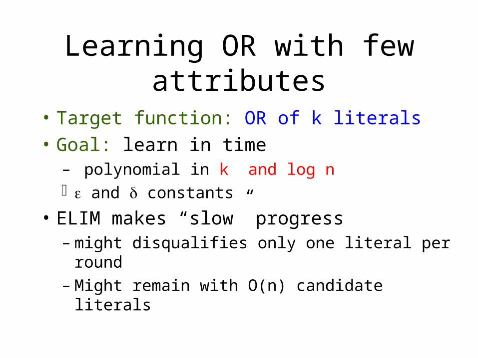
ELIM: Algorithm for learning OR

• Keep a list of all candidate literals• For every example whose classification is 0:

– Erase all the literals that are 1.

• Correctness:– Our hypothesis h: An OR of our set of literals.– Our set of literals includes the target OR literals.– Every time h predicts zero: we are correct.

• Sample size: – m > (1/) ln (3n/)= O (n/ +1/ ln (1/)

Set Cover - Definition

• Input: S1 , … , St and Si U

• Output: Si1, … , Sik and j Sjk=U

• Question: Are there k sets that cover U?

• NP-complete

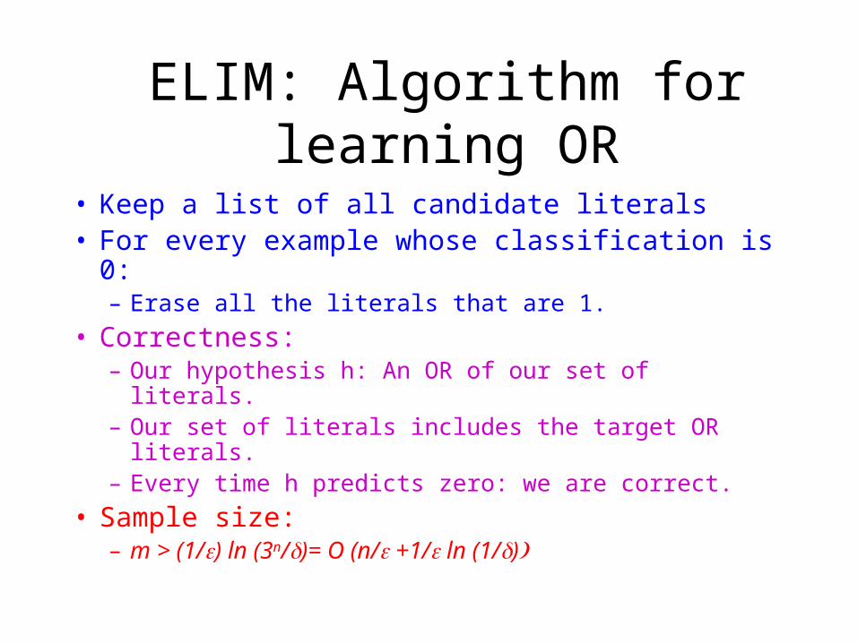
Set Cover: Greedy algorithm

• j=0 ; Uj=U; C=• While Uj

– Let Si be arg max |Si Uj|

– Add Si to C

– Let Uj+1 = Uj – Si

– j = j+1

Set Cover: Greedy Analysis

• At termination, C is a cover.

• Assume there is a cover C* of size k.

• C* is a cover for every Uj

• Some S in C* covers Uj/k elements of Uj

• Analysis of Uj: |Uj+1| |Uj| - |Uj|/k

• Solving the recursion.

• Number of sets j k ln ( |U|+1)

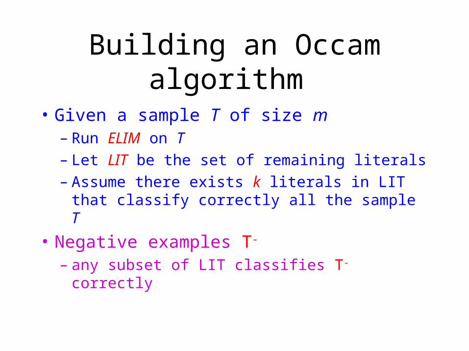
Building an Occam algorithm

• Given a sample T of size m– Run ELIM on T – Let LIT be the set of remaining literals– Assume there exists k literals in LIT that

classify correctly all the sample T

• Negative examples T-

– any subset of LIT classifies T- correctly

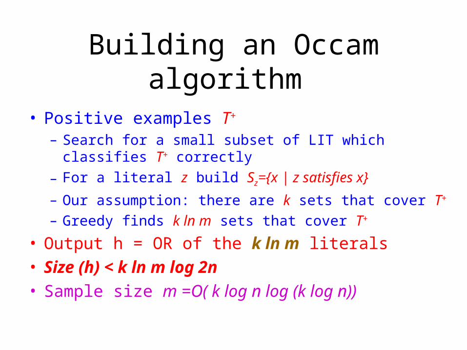
Building an Occam algorithm

• Positive examples T+ – Search for a small subset of LIT which classifies T+ correctly

– For a literal z build Sz={x | z satisfies x}

– Our assumption: there are k sets that cover T+

– Greedy finds k ln m sets that cover T+

• Output h = OR of the k ln m literals • Size (h) < k ln m log 2n• Sample size m =O( k log n log (k log n))

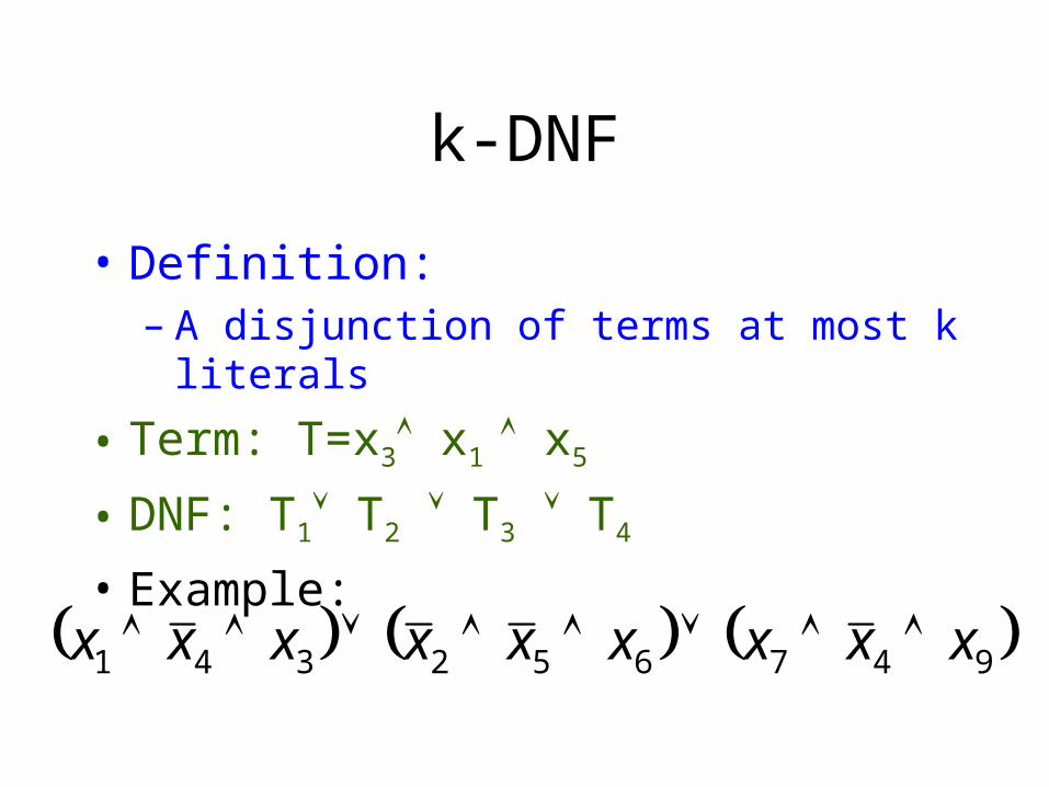
k-DNF

• Definition:– A disjunction of terms at most k literals

• Term: T=x3 x1 x5

• DNF: T1 T2 T3 T4

• Example:

947652341 xxxxxxxxx

Learning k-DNF

• Extended input:– For each AND of k literals define a “new” input T– Example: T=x3 x1 x5

– Number of new inputs at most (2n)k

– Can compute the new input easily in time k(2n)k

– The k-DNF is an OR over the new inputs.– Run the ELIM algorithm over the new inputs.

• Sample size O ((2n)k/ +1/ ln (1/) • Running time: same.

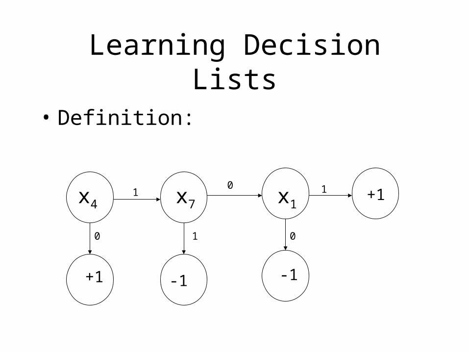
Learning Decision Lists

• Definition:

x4 x7 x1

+1 -1 -1

+11

1

1

0

0

0

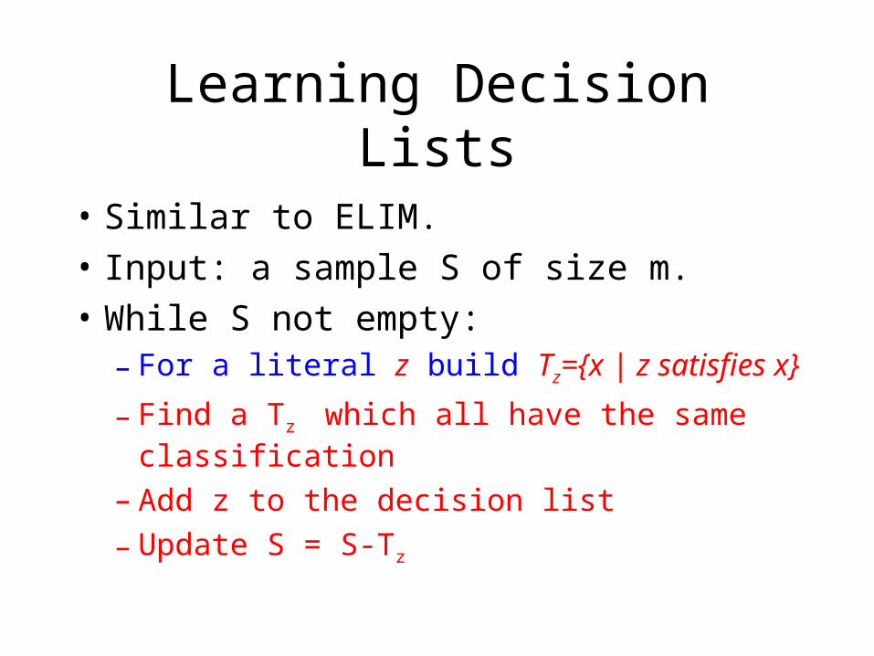
Learning Decision Lists

• Similar to ELIM.

• Input: a sample S of size m.

• While S not empty:– For a literal z build Tz={x | z satisfies x}

– Find a Tz which all have the same classification

– Add z to the decision list

– Update S = S-Tz

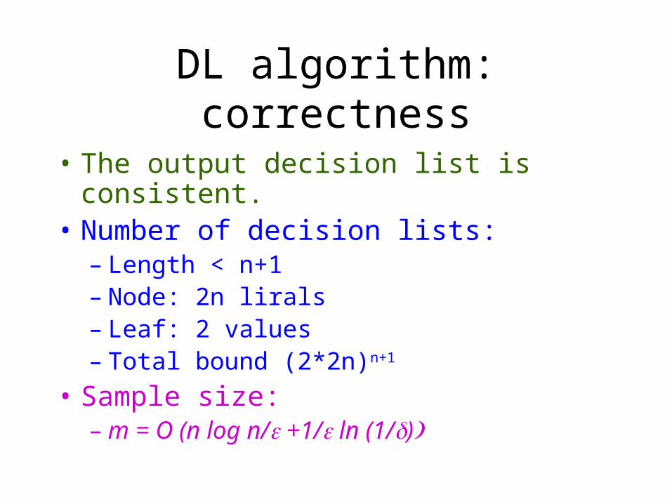
DL algorithm: correctness

• The output decision list is consistent.• Number of decision lists:

– Length < n+1– Node: 2n lirals– Leaf: 2 values– Total bound (2*2n)n+1

• Sample size:– m = O (n log n/ +1/ ln (1/)

k-DL

• Each node is a conjunction of k literals

• Includes k-DNF (and k-CNF)

x4 x2

+1 -1 -1

+11 1 1

0 0 0

x3 x1 x5 x7

Learning k-DL

• Extended input:– For each AND of k literals define a “new” input– Example: T=x3 x1 x5

– Number of new inputs at most (2n)k

– Can compute the new input easily in time k(2n)k

– The k-DL is a DL over the new inputs.– Run the DL algorithm over the new inputs.

• Sample size • Running time

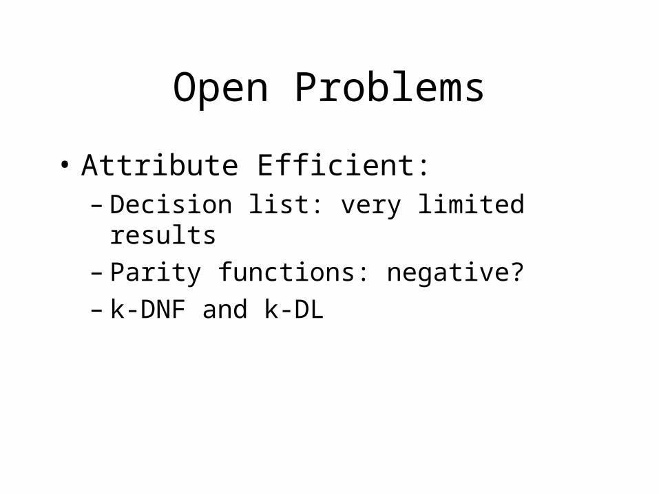
Open Problems

• Attribute Efficient:– Decision list: very limited results– Parity functions: negative?– k-DNF and k-DL

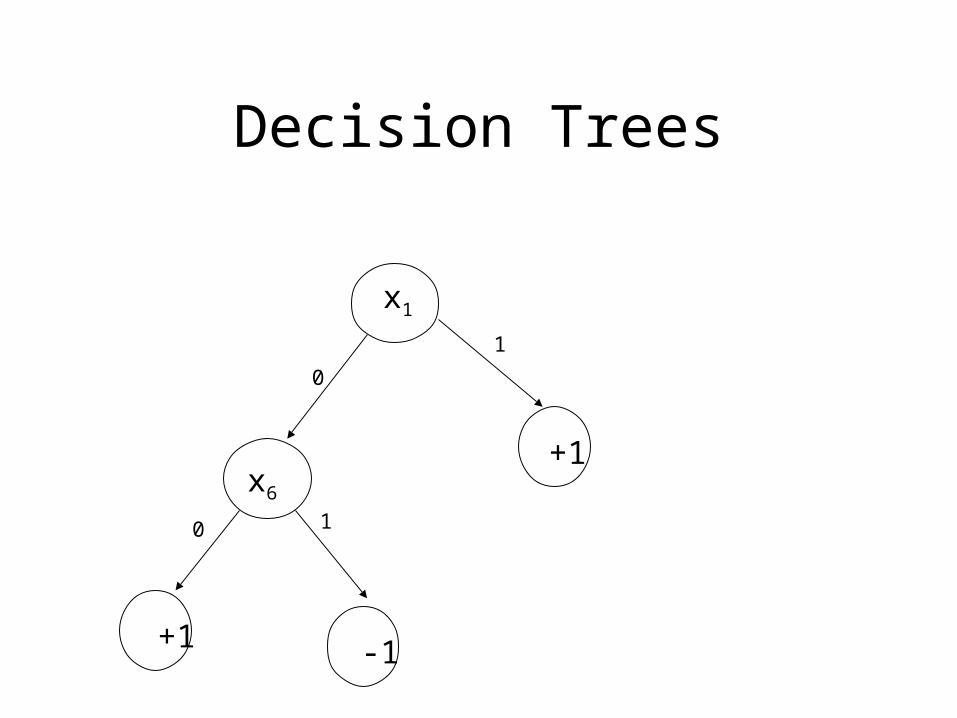
Decision Trees

x1

x6

+1 -1

+1

1

1

0

0

Learning Decision Trees Using DL

• Consider a decision tree T of size r.• Theorem:

– There exists a log (r+1)-DL L that computes T.

• Claim: There exists a leaf in T of depth log (r+1).• Learn a Decision Tree using a Decision List• Running time: nlog s

– n number of attributes– S Tree Size.

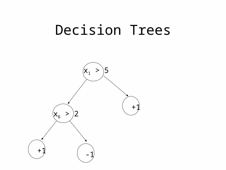
Decision Trees

x1 > 5

x6 > 2

+1 -1

+1

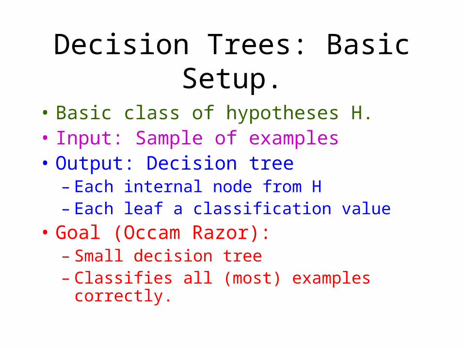
Decision Trees: Basic Setup.

• Basic class of hypotheses H.• Input: Sample of examples• Output: Decision tree

– Each internal node from H– Each leaf a classification value

• Goal (Occam Razor):– Small decision tree– Classifies all (most) examples correctly.

Decision Tree: Why?

• Efficient algorithms:– Construction.– Classification

• Performance: Comparable to other methods

• Software packages:– CART– C4.5 and C5

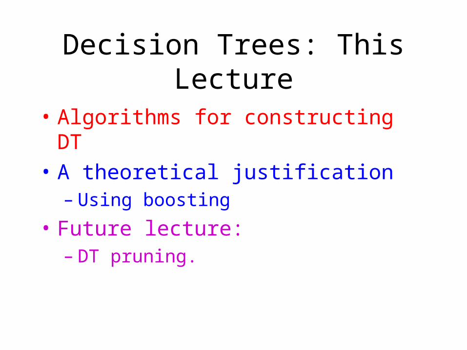
Decision Trees: This Lecture

• Algorithms for constructing DT

• A theoretical justification– Using boosting

• Future lecture:– DT pruning.

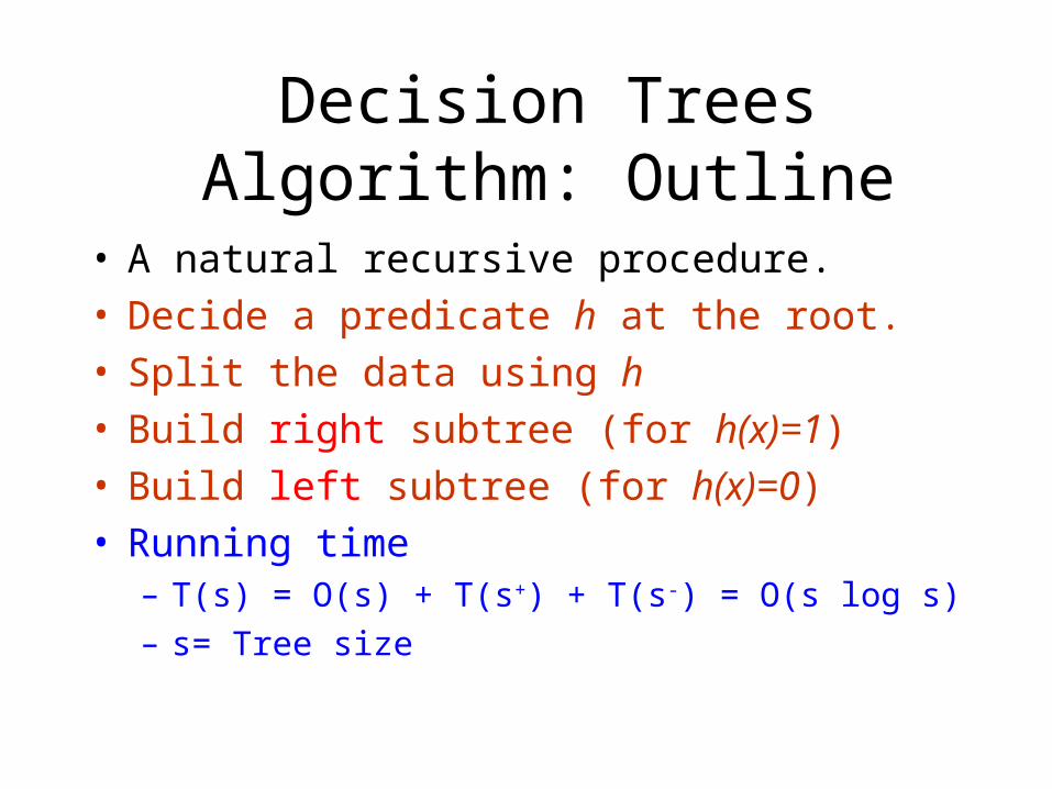
Decision Trees Algorithm: Outline

• A natural recursive procedure.• Decide a predicate h at the root.• Split the data using h• Build right subtree (for h(x)=1)• Build left subtree (for h(x)=0)• Running time

– T(s) = O(s) + T(s+) + T(s-) = O(s log s)

– s= Tree size

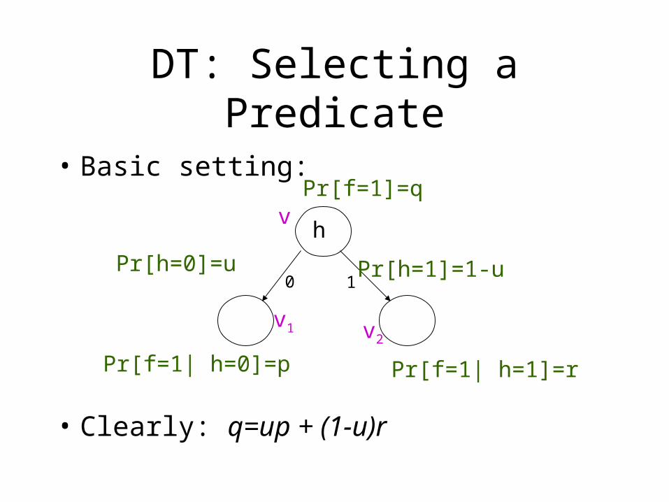
DT: Selecting a Predicate

• Basic setting:

• Clearly: q=up + (1-u)r

h

Pr[f=1]=q

Pr[f=1| h=0]=p Pr[f=1| h=1]=r

0 1Pr[h=0]=u Pr[h=1]=1-u

v

v1 v2

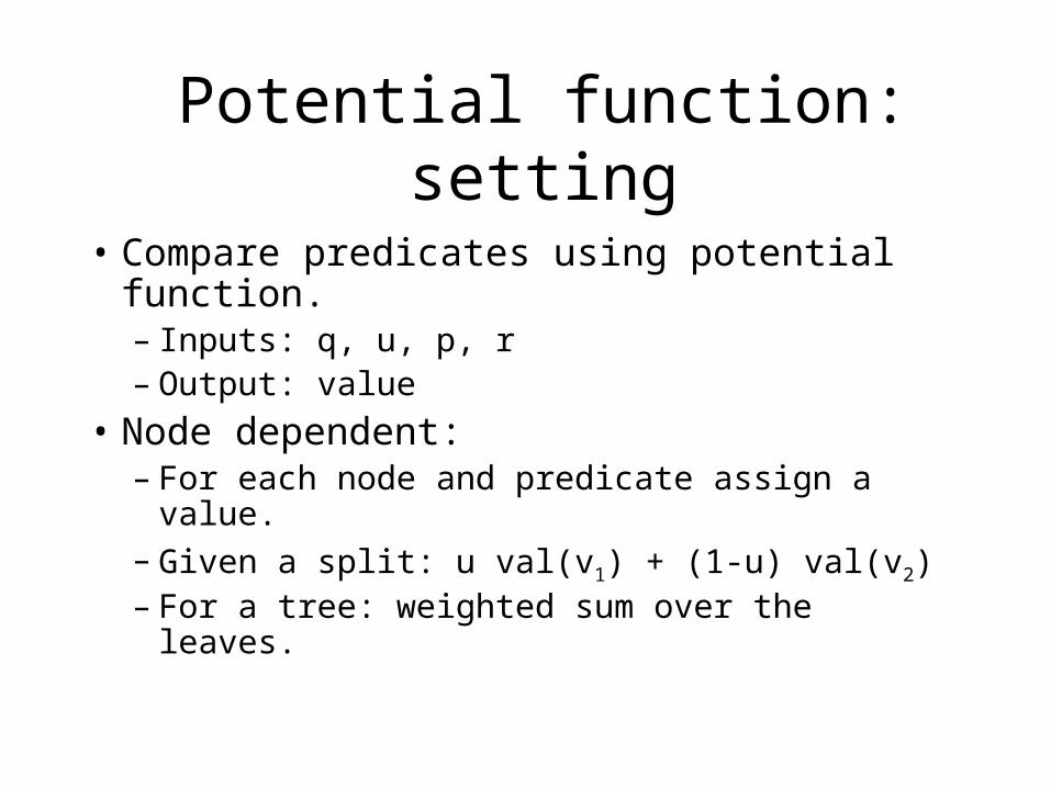
Potential function: setting

• Compare predicates using potential function.– Inputs: q, u, p, r– Output: value

• Node dependent:– For each node and predicate assign a value.– Given a split: u val(v1) + (1-u) val(v2)– For a tree: weighted sum over the leaves.

PF: classification error

• Let val(v)=min{q,1-q}– Classification error.

• The average potential only drops

• Termination:– When the average is zero– Perfect Classification

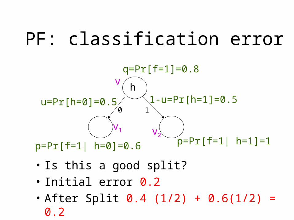
PF: classification error

• Is this a good split?

• Initial error 0.2

• After Split 0.4 (1/2) + 0.6(1/2) = 0.2

h

q=Pr[f=1]=0.8

p=Pr[f=1| h=0]=0.6

0 1u=Pr[h=0]=0.5

v

v1 v2

1-u=Pr[h=1]=0.5

p=Pr[f=1| h=1]=1

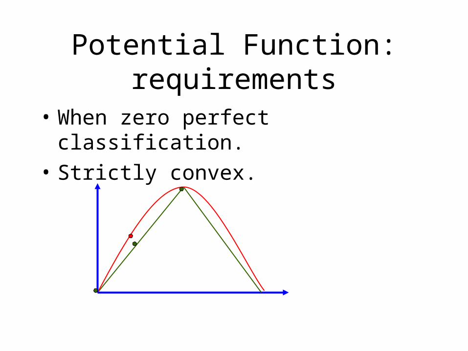
Potential Function: requirements

• When zero perfect classification.

• Strictly convex.

Potential Function: requirements

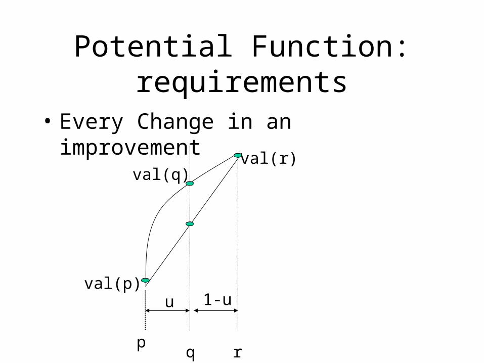
• Every Change in an improvement

pq r

u 1-u

val(q)

val(p)

val(r)

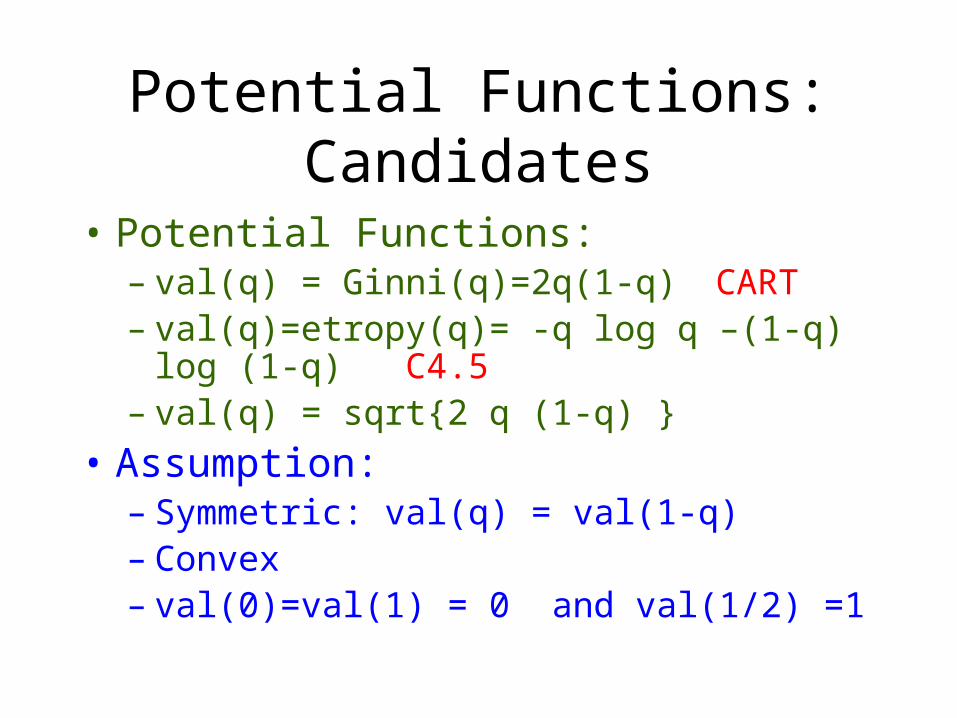
Potential Functions: Candidates

• Potential Functions:– val(q) = Ginni(q)=2q(1-q) CART– val(q)=etropy(q)= -q log q –(1-q) log (1-q) C4.5– val(q) = sqrt{2 q (1-q) }

• Assumption:– Symmetric: val(q) = val(1-q)– Convex– val(0)=val(1) = 0 and val(1/2) =1

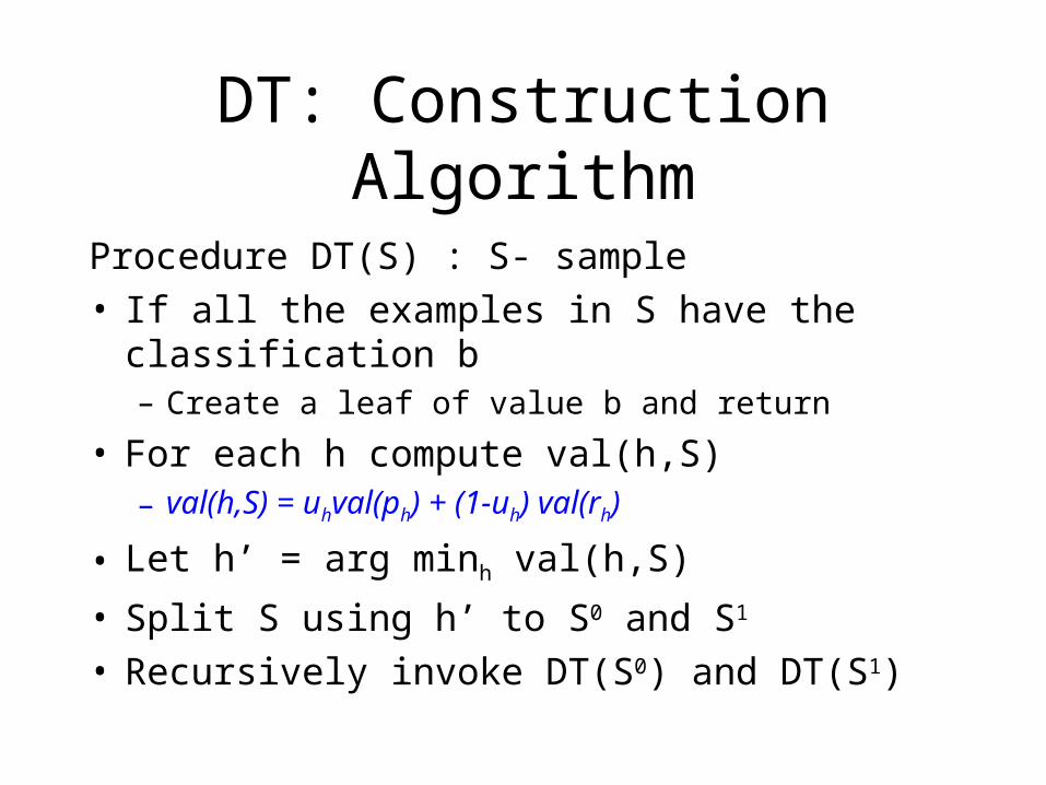
DT: Construction Algorithm

Procedure DT(S) : S- sample• If all the examples in S have the classification b

– Create a leaf of value b and return

• For each h compute val(h,S)– val(h,S) = uhval(ph) + (1-uh) val(rh)

• Let h’ = arg minh val(h,S)

• Split S using h’ to S0 and S1

• Recursively invoke DT(S0) and DT(S1)

DT: Analysis

• Potential function:– val(T) = v leaf of T Pr[v] val(qv)

• For simplicity: use true probability• Bounding the classification error

– error(T) val(T)– study how fast val(T) drops

• Given a tree T define T(l,h) where – h predicate– l leaf.

T

h

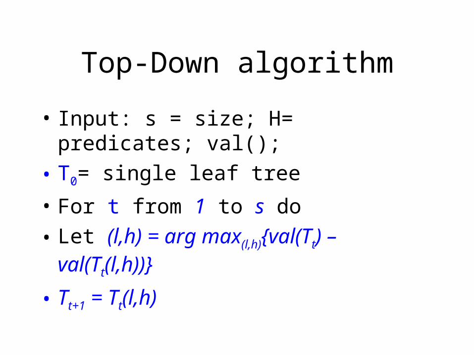
Top-Down algorithm

• Input: s = size; H= predicates; val();

• T0= single leaf tree

• For t from 1 to s do

• Let (l,h) = arg max(l,h){val(Tt) – val(Tt(l,h))}

• Tt+1 = Tt(l,h)

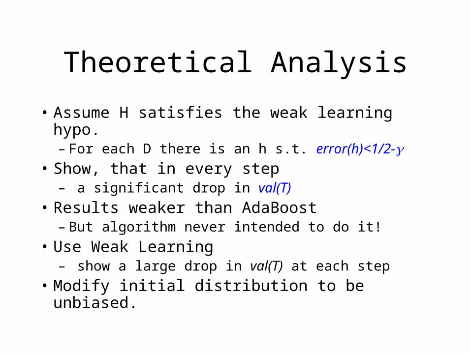
Theoretical Analysis

• Assume H satisfies the weak learning hypo.– For each D there is an h s.t. error(h)<1/2-

• Show, that in every step– a significant drop in val(T)

• Results weaker than AdaBoost– But algorithm never intended to do it!

• Use Weak Learning – show a large drop in val(T) at each step

• Modify initial distribution to be unbiased.

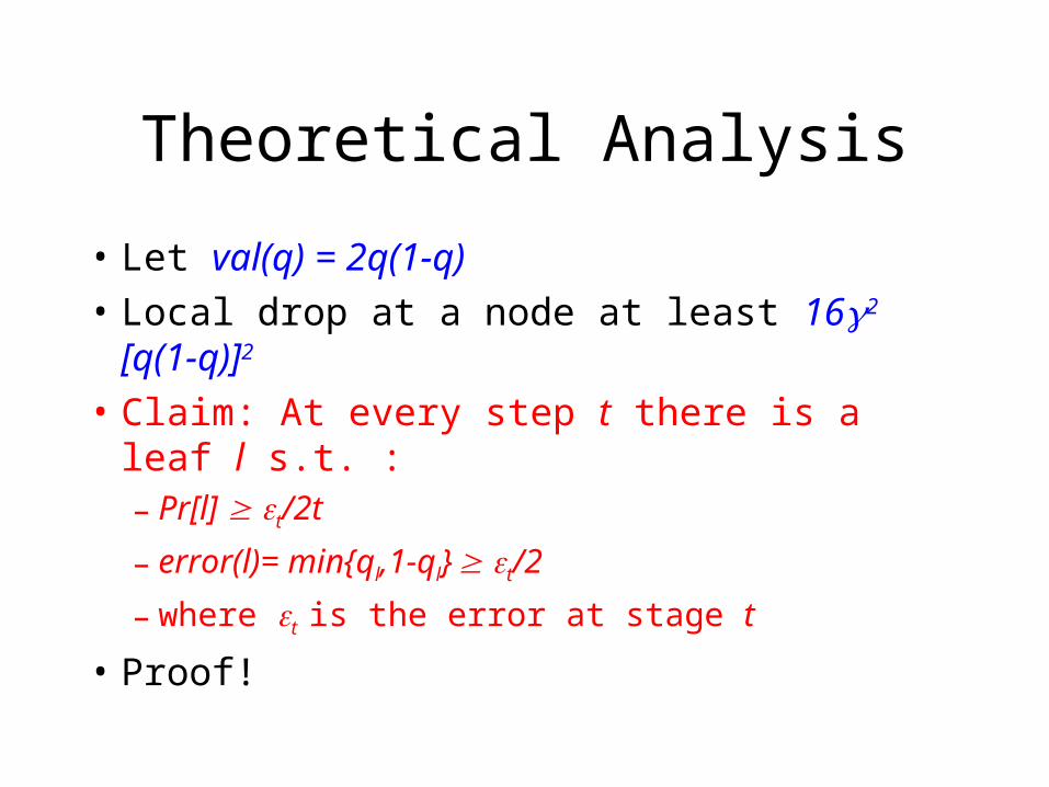
Theoretical Analysis

• Let val(q) = 2q(1-q)

• Local drop at a node at least 162 [q(1-q)]2

• Claim: At every step t there is a leaf l s.t. :– Pr[l] t/2t

– error(l)= min{ql,1-ql} t/2

– where t is the error at stage t

• Proof!

Theoretical Analysis

• Drop at time t at least:– Pr[l] 2 [ql (1-ql)]2 2 t

3 / t

• For Ginni index– val(q)=2q(1-q)– q q(1-q) val(q)/2

• Drop at least O(2 [val(qt)]3/ t )

Theoretical Analysis

• Need to solve when val(Tk) < • Bound k.

• Time exp{O(1/2 1/ 2)}

Something to think about

• AdaBoost: very good bounds

• DT Ginni Index : exponential

• Comparable results in practice

• How can it be?