Embed Size (px)
Citation preview
TITLE PAGE
Decision Support System of Coal Mine Planning
Using System Dynamics Model
To the Faculty of Geosciences, Geoengineering and Mining
of the Technische Universität Bergakademie Freiberg
approved
THESIS
to attain the academic degree of
Doktor-Ingenieur
(Dr.-Ing.)
submitted
by M.Sc. Phongpat Sontamino
born on the 03.11.1978 in Nakhon Si Thammarat/ Thailand
Reviewers: Prof. Dr. Carsten Drebenstedt, Germany
Prof. Dr. Pitsanu Bunnaul, Thailand
Prof. Dr. Horst Brezinski, Germany
Date of the award 05.12.2014


III
ABSTRACT
Coal is a fossil fuel mineral, which is presently a major source of electricity and energy
to industries. From past to present, there are many coal reserves around the world and
large scale coal mining operates in various areas such as the USA, Russia, China,
Australia, India, and Germany, etc [1, 2]. Thailand’s coal resources can be found in
many areas; there are lignite mining in the north of Thailand, the currently operational
Mae Moh Lignite Mine [3, 4], and also coal reserves in the south of Thailand, such as
Krabi and Songkhla [5], where mines are not yet operating. The main consumption of
coal is in electricity production, which increases annually. In 2019, the Thai
Government and Electricity Generating Authority of Thailand (EGAT) plans to run a
800 MW coal power plant at Krabi [6], which may run on imported coal, despite there
being reserves of lignite at Krabi [5]; the use of domestic coal is a last option because of
social and environmental concerns about the effects of coal mining. There is a modern
trend in mining projects, the responsibility of mining should cover not only the mining
activity, but the social and environmental protection and mine closure activities which
follow [6]. Thus, the costs and decisions taken on by the mining company are
increasingly complicated.
To reach a decision on investment in a mining project is not easy; it is a complex
process in which all variables are connected [7]. Particularly, the responsibility of coal
mining companies to society and the environment is a new topic. Thus, a tool to help to
recognize and generate information for decision making is in demand and very
important. In this thesis, the system dynamics model of coal mine planning is made by
using Vensim Software [8] and specifically designed to encompass many variables
during the period of mining activity until the mine closure period. The decisions use
economic criteria such as Net Present Value (NPV) [9], Net Cash Flow (NCF), Payback
Period (PP) [10], and Internal Rate of Return (IRR), etc.
Consequently, the development of the decision support system of coal mine planning as
a tool is proposed. The model structure covers the coal mining area from mine reserves
to mine closure. It is a fast and flexible tool to perform sensitivity analysis, and to
determine an optimum solution. The model results are clear and easily understandable
on whether to accept or reject the coal mine project, which helps coal mining companies

IV
make the right decisions on their policies, economics, and the planning of new coal
mining projects.
Furthermore, the model is used to analyse the case study of the Krabi coal-fired power
plant in Thailand, which may possibly use the domestic lignite at Krabi. The scenario
simulations clearly show some potential for the use of the domestic lignite. However,
the detailed analysis of the Krabi Lignite Mine Project case shows the high possible
risks of this project, and that this project is currently not feasible. Thus, the model helps
to understand and confirm that the use of domestic lignite in Krabi for the Krabi Coal
Power Plant Project is not suitable at this time. Therefore, the best choice is imported
coal from other countries for supporting the Krabi Coal Power Plant Project.
Finally, this tool successfully is a portable application software, which does not need to
be installed on a computer, but can run directly in a folder of the existing application.
Furthermore, it supports all versions of Windows OS.

V
ACKNOWLEDGEMENTS
I would like to express my deepest and warmest thanks and gratitude to my supervisor
Prof. Dr. Carsten Drebenstedt for his kind supervision, valuable advice, guidance, for
reviewing this thesis, and his support throughout my study in the Federal Republic of
Germany. In addition, special thanks to my reviewers and all PhD committees, Prof. Dr.
Horst Brezinski, Prof. Dr. Pitsanu Bunnaul, Prof. Dr. Mohamed Amro, Prof. Dr.
Bernhard Jung, and Prof. Dr. Carsten Felden, for all recommendations in this thesis.
I address my hearty and special thanks and gratitude to my home country (Thailand) for
granting me the scholarship to do a doctorate at the TU Bergakademie Freiberg. I thank
all of the staff of the Thai embassy in Berlin, and all of the scholarship staff in Thailand
for their aid in providing support during the time I have spent in Freiberg, Germany.
Many thanks are directed to my colleagues in the Department of Mining and Materials
Engineering, Faculty of Engineering, Prince of Songkla University; and especially to
Asst. Prof. Dr. Manoon Masniyom for their advice and support of everything during my
study.
I am also greatly thankful to all the colleagues and staff of the Institute of Mining and
Special Civil Engineering; Dr. Günter Lippmann, Dr. Pham Van Hoa, Mr. Richard A.
Eichler, Mr. Martin Pfütze, Mr. Inthanongsone Inthavongsa and others, for their
kindness and encouragement during my studies.
Many thanks must go to the Mae Moh Lignite Mine in Thailand, especially to Mr.
Ampon Kitichotkul, Mr. Titipun Phongramon, and others for support data and allowing
me to use all of the information to form the case study in this thesis.
I address my sincere thanks to my parents and all my family members for their
continued support, education, and tolerance.
Finally, special thanks to my wife Mrs. Chutikarn Sontamino, for her great love,
forbearance, tolerance, and encouragement. I owe my wife a debt of gratitude for her
patience, understanding, and for taking care of me for the years I studied here. She also
gives me a special gift, my adorable and healthy boy, Mr. Porranat Sontamino.

VI
TABLE OF CONTENTS
Title Page .......................................................................................................................... I
Abstract ......................................................................................................................... III
Acknowledgements ......................................................................................................... V
Table of Contents ......................................................................................................... VI
List of Figures ............................................................................................................ VIII
List of Tables ................................................................................................................ XI
List of Abbreviatio ...................................................................................................... XII
1 Introduction ......................................................................................................... 1
1.1 Stage of Coal Mining System ..................................................................... 1
1.2 Thailand Coal Mining and Problems .......................................................... 5
1.3 Objectives .................................................................................................... 8
1.4 Remarks ....................................................................................................... 8
1.5 Thesis Outlines ............................................................................................ 9
2 Literature Reviews ............................................................................................ 11
2.1 Multi-method Simulation Approach ......................................................... 11
2.2 System Dynamics Theory and Modelling ................................................. 12
2.2.1 Overview ................................................................................................... 12 2.2.2 The System Dynamics Approach .............................................................. 13 2.2.3 SD Modelling and Simulation ................................................................... 14 2.2.4 Feedback Thinking .................................................................................... 15 2.2.5 System Structure ....................................................................................... 17
2.3 System Dynamics Modelling Software Selection ..................................... 19
2.4 System Dynamics Model and Decision Making in Mining ...................... 21
2.5 Chapter Conclusion ................................................................................... 25
3 Research Methodology and Model Development ............................................... 27
3.1 Research Approach ................................................................................... 27
3.2 Develop SD Model .................................................................................... 29
3.2.1 Causal Loop Diagram ............................................................................... 29 3.2.2 System Dynamics Model .......................................................................... 32
3.3 Chapter Conclusion ................................................................................... 42
4 Case Study Krabi Lignite Mine ....................................................................... 43
4.1 Coal Mining in Thailand ........................................................................... 43
4.2 Analysed Variables ................................................................................... 46
4.2.1 Mining Variables ....................................................................................... 46 4.2.2 Economic Decision Variables ................................................................... 51 4.2.3 Exogenous Variables ................................................................................. 52
VII
4.3 Model Verification .................................................................................... 59
4.3.1 Logical checking ....................................................................................... 60 4.3.2 Model structure checking ......................................................................... 60 4.3.3 Model unit checking ................................................................................. 61 4.3.4 Compared calculation result with real data .............................................. 61
4.4 Simulation Conditions Setup .................................................................... 66
4.4.1 Sensitivity Analysis Conditions ................................................................ 67 4.4.2 Scenario Simulation Conditions ............................................................... 67 4.4.3 Optimum Funding Conditions .................................................................. 69
5 Case Study Simulation Results and Discussion ............................................. 70
5.1 Simulation Results of Krabi Lignite Mine Project ................................... 70
5.1.1 Sensitivity Analysis Results ..................................................................... 70 5.1.2 Scenario Simulation Results ..................................................................... 81 5.1.3 Optimum Funding Result ......................................................................... 91
5.2 Discussion of Krabi Lignite Mine Project ................................................ 94
5.2.1 The Comparison of Scenarios Simulation ................................................ 94 5.2.1 Electricity Price Effect on Krabi Lignite Mine Project ............................ 98 5.2.2 Economic Value of Krabi Lignite Mine Project ..................................... 100 5.2.3 The Alternative of Krabi Coal Power Plant Project ............................... 102
6 Development of Application Interface .......................................................... 105
6.1 Application Interface Result ................................................................... 106
6.1.1 Scenario Simulation Menu ..................................................................... 108 6.1.2 Sensitivity Analysis Simulation Menu ................................................... 111
6.2 Application Installation and Usage ......................................................... 114
7 Summary and Recommendation ................................................................... 116
7.1 Summary ................................................................................................. 116
7.2 Recommendations for Further Research ................................................ 117
References .................................................................................................................... 119
I. Appendix 1: Background Information ......................................................... 124
World Coal Status and Coal Mining ................................................................. 124
Social and Environmental Problems of Coal Mining ....................................... 139
Mine Economic Valuation ................................................................................ 143
II. Appendix 2: Additional Information Table ................................................. 166
III. Appendix 3: Model Equations Code ............................................................. 173
IV. Appendix 4: Application Code ...................................................................... 195

VIII
LIST OF FIGURES
Figure 1.1: Top 10 world coal reserves (2008) [1] ................................................................ 1
Figure 1.2: World energy consumption by sources (1987-2012) [13] .................................... 2
Figure 1.3: Resources to production ratio (R/P ratio) [13] ..................................................... 2
Figure 1.4: World energy source of electricity [14] ................................................................ 3
Figure 1.5: Environmental impact of mining (example) [6] ................................................. 4
Figure 1.6: Mae Moh Lignite Mine and Power Plant [4] ...................................................... 5
Figure 1.7: The simple process of surface coal mining in Thailand (modified) [18].............. 6
Figure 1.8: Sources of electricity in Thailand and the world [14] .......................................... 7
Figure 2.1: Forrester’s organizing framework for the system structure .......................... 17
Figure 2.2: The conceptual model of C. Roumpos, et.al. [7] .............................................. 21
Figure 2.3: Fan’s flow diagram of coal production and supply [62] ..................................... 22
Figure 2.4: Concept of the Caselles-Moncho’s model [63] .................................................. 23
Figure 2.5: Principle of the O’Regan model diagram [64] ................................................... 24
Figure 3.1: Research approach and SDM development procedure ................................. 27
Figure 3.2: Causal loop diagram of mine planning system ............................................. 29
Figure 3.3: The conceptual diagram for mine planning decision (Narrow Sense) ......... 30
Figure 3.4: The conceptual diagram for mine planning decision (Wider Sense) ............ 31
Figure 3.5: The conceptual diagram for mine planning decision (Widest Sense) .......... 31
Figure 3.6: SDM Structure of Mining System ................................................................ 34
Figure 3.7: SDM Structure of Economic Decision ......................................................... 36
Figure 3.8: SDM Structure of Total Cost and Worker Estimation ................................. 37
Figure 3.9: SDM Structure of Operating Cost Estimation .............................................. 38
Figure 3.10: SDM Structure of Capital Cost Estimation ................................................ 40
Figure 3.11: SDM Structure of Power Plant Economic Value ....................................... 41
Figure 4.1: Coal potential resources and reserves of Thailand (Modified) [65] ................... 43
Figure 4.2: Coal Production in Thailand (1987-2012) (Revised) [66, 67] ................................. 45
Figure 4.3: Coal Consumption in Thailand (1987-2012) (Revised) [66, 67] ............................. 46
Figure 4.4: Position map of Krabi coal reserves (Modified) [70] ......................................... 47
Figure 4.5: Lignite Price (1949-2011) [36] ........................................................................... 52
Figure 4.6: Histogram of Lignite Price [36] .......................................................................... 53
Figure 4.7: Interest Rate Policy of Thailand (2005-2014) [81] ............................................. 57
Figure 4.8: Annual Inflation Rate of Thailand (1990-2013) [83] ......................................... 58
Figure 4.9: Lending Interest Rate of Thailand (2000-2012) [84] ......................................... 58

IX
Figure 4.10: Model Structure Checking Result .............................................................. 60
Figure 4.11: Model Unit Checking Result ...................................................................... 61
Figure 4.12: Mae Moh Lignite Mine (Modified) [68] .......................................................... 62
Figure 4.13: Comparison of Mae Moh Production by Real Data and Simulation ......... 65
Figure 4.14: Procedure of Simulation Result Making .................................................... 66
Figure 4.15: Lignite Price Trend Forecasting (Modified) [88] ............................................. 69
Figure 5.1: Sensitivity Analysis Result of Lignite Price ................................................ 71
Figure 5.2: Sensitivity Analysis Result of Stripping Ratio............................................. 72
Figure 5.3: Sensitivity Analysis Result of Coal Heating Value ..................................... 73
Figure 5.4: Sensitivity Analysis Result of Tax Rate ....................................................... 75
Figure 5.5: Sensitivity Analysis Result of Discount Rate .............................................. 76
Figure 5.6: Sensitivity Analysis Result of Unit S&EP Cost ........................................... 77
Figure 5.7: Sensitivity Analysis Result of Unit Mine Closure Cost ................................. 78
Figure 5.8: Sensitivity Analysis Result of Deposit Interest Rate ................................... 79
Figure 5.9: Summary sensitivity analysis of each variable to NPV Balance ................. 80
Figure 5.10: The decision criteria result of the Constant Price Scenario ....................... 82
Figure 5.11: The decision criteria result of the Normal Forecasting Price Scenario ...... 85
Figure 5.12: The decision criteria result of the Worst Forecasting Price Scenario ........ 88
Figure 5.13: The decision criteria result of the Best Forecasting Price Scenario ........... 90
Figure 5.14: Cumulative mining fund a long period of mine life ................................... 92
Figure 5.15: Mining fund cash flow comparison............................................................ 92
Figure 5.16: The optimum mining fund on the Normal Forecasting Price Scenario ..... 93
Figure 5.17: The comparison of scenario simulation graph results I ............................. 95
Figure 5.18: The comparison of scenario simulation graph results II ............................ 96
Figure 5.19: The comparison of scenario simulation graph results III ........................... 97
Figure 5.20: Krabi power plant decision condition ...................................................... 100
Figure 5.21: Economic value of society by royalties and corporate tax ....................... 101
Figure 5.22: Unit of power plant fuel cost and profit comparison ............................... 103
Figure 6.1: Interface Diagram of DSS-CMPv1.0 .............................................................. 106
Figure 6.2: Cover Interface of DSS-CMPv1.0 .................................................................. 107
Figure 6.3: Acknowledgements Interface of DSS-CMPv1.0 ............................................. 107
Figure 6.4: Main Menu Interface of DSS-CMPv1.0 ......................................................... 108
Figure 6.5: Scenario Simulation Conditions Setup Interface of DSS-CMPv1.0 .................. 109
Figure 6.6: Scenario Result I Interface of DSS-CMPv1.0 ................................................. 109

X
Figure 6.7: Scenario Result II Interface of DSS-CMPv1.0 ................................................ 110
Figure 6.8: Scenario Result III Interface of DSS-CMPv1.0 ............................................... 110
Figure 6.9: Sensitivity Analysis Condition Setup Interface of DSS-CMPv1.0..................... 111
Figure 6.10: DSS-CMPv1.0 Sensitivity Graph of Net Cash Balance (example) .................. 112
Figure 6.11: DSS-CMPv1.0 Sensitivity Graph of NPV Balance (example) ........................ 113
Figure 6.12: DSS-CMPv1.0 Sensitivity Graph of Cumulative Mining Fund (example) ...... 113
Figure 6.13: Application password protection .............................................................. 115
Figure I.1: Pyramid of the USA coal resources and reserves [22] ...................................... 124
Figure I.2: Resource to production ratio 2013 [12] ............................................................. 127
Figure I.3: Coal potential and occurrence around the world [24] ....................................... 127
Figure I.4: Distribution of proved reserves in 1992, 2002, and 2012 [13] .......................... 128
Figure I.5: Surface coal mining method (example) [27] ..................................................... 129
Figure I.6: Longwall mining method [32] ........................................................................... 130
Figure I.7: Coal production and consumption by region [13] ............................................. 131
Figure I.8: Coal consumption per capita 2012 [13] ............................................................ 133
Figure I.9: The global coal price 1949 - 2011 (Modified) [36] ........................................... 135
Figure I.10: Cost of fossil-fuel receipts at electric generating plants 1973-2012 [35] ........ 136
Figure I.11: Coal production, consumption, import, and export in USA. [38] ................... 138
Figure I.12: Bian’s conceptual framework for solving the environmental issues [11] ....... 140
XI
LIST OF TABLES
Table 2.1: List of system dynamics modelling software (Modified) [60] ............................ 19
Table 2.2: The analytical comparison of the top 5 of system dynamics software [60] ........ 20
Table 4.1: Analytical coal quality of Krabi [5] ................................................................... 48
Table 4.2: Analytical coal resources in Krabi [5] ............................................................... 49
Table 4.3: Statistical analysis of the coal price in US$/t [36] ............................................... 53
Table 4.4: Energy plan of Thailand 2012-2030 [74] ............................................................ 54
Table 4.5: Statistical analysis of the discount rate [80, 82 , 84] ....................................................... 59
Table 4.6: Mechanical properties of coal and overburden in Mae Moh Mine [69] .............. 64
Table 4.7: List of input variable values used for sensitivity analysis ............................. 67
Table 4.8: List of highlight input variable for Constant Price Scenario ......................... 68
Table 4.9: Criteria of the optimum condition ................................................................. 69
Table 5.1: Summary critical point in each scenario ....................................................... 98
Table 5.2: Summary alternative of Krabi Coal Power Plant Project ............................ 104
Table I.1: Top 5 world hydrocarbon energy reserves by country (2011) [22] ................... 128
Table I.2: Top 5 world coal reserves by countries (2013) [12] .......................................... 128
Table I.3: Top 5 world coal producers (2004-2012) [33, 34] .................................................. 132
Table I.4: Top 5 world coal consumers (2008-2013) [12] .................................................. 132
Table I.5: Coal average sales prices (2011) [35] ................................................................ 134
Table I.6: Top 5 world coal importing countries (2006-2012) [37] ................................... 137
Table I.7: Top 5 world coal exporting countries (2006-2012) [39] .................................... 138
Table I.8: Mining costs for ore and waste [43] ................................................................... 145
Table II.1: The lignite production of Thailand (1987-2012) [66, 67] ...................................... 166
Table II.2: The lignite consumption of Thailand (1987-2012) [66, 67] ................................... 167
Table II.3: List of input parameter values in Constant Price Scenario ......................... 168
Table II.4: List of input parameters of the model ......................................................... 169
Table II.5: List of auxiliary input parameter unit converters ........................................ 169
Table II.6: List of auxiliary input parameters of unit cost (k.xi) and power (n.xi) ....... 170
Table II.7: List of the output parameters in the model ................................................. 170
XII
LIST OF ABBREVIATIONS
Ac Required Area for Milling Plant PV Present Value
ADJTIM Adjustment Time DSS Decision Support System
Ap Required Area for Soil Dumping Oc Operating Costs
Ars Required Area of Maintenance Shop t Tonne/Tonnes/Metric ton
Ave. Average kcal Kilo Calories
BBOE Billion Barrels of Oil Equivalent Cpcp Cost of Primary Crusher Plant
BTU British Thermal Unit Nat Number of Administrative and Technical
Staffs
Cal Calories m3 Cubic Meters
Cc Clearing Costs S.D. Standard Deviation
Cce Communication and Electrical Distribution
Costs
kWh Kilowatt Hour
Cde Drilling Equipment Cost Gcpd General Service Cost Per Day
CFA Cash Flow Analysis q Imputed Interest
Cle Cost of Shovel Supplemented Scpd Surface Service Cost
Cpmf Constructing and Equipping Shop Costs At (0) Periodic Amount of The Cash-layout Costs
Crs Fuelling System Costs DCF Discount Cash Flow
Css Soil Stripping Cost Dcpd Drilling Cost Per Day
Cws Waste Stripping Cost Bcpd Blasting Cost Per Day
DSSN Dry Small Steam Nuts Cgc Cost of Gyratory Crushers
EGAT Electricity Generating Authority of
Thailand
Aof Administrative Office Area Required
EHIA Environmental Health Impact Assessment S&EP Social and Environmental Protection
FV Future Value N/A Not Available
G&A General and Administrative Cof Cost of Office Building
Hec Haulage Equipment Costs t Time
i Discount Rate GWh Gigawatt Hour
IPP Independent Power Producers SPP Small Power Producers
IRR Internal Rate of Return Ar Access Road Costs of Milling Plant
J Joules WACC The Weighted Average Cost of Capital
kg Kilogram g Gramm
Max. Maximum Gcal Giga Calories
MEP Materials, Expenses, and Power Csh Cost of Maintenance Shop
MFR Mining Fund Rate NCF Net Cash Flow
Min. Minimum US$ United States Dollars ($)
MIT Massachusetts Institute of Technology DYNAMO Dynamics Model Software
MJ Mega joules kJ Kilojoules
MTOE Million Tonnes of Oil Equivalent s Second
MW Megawatt Cu Volume of Rock Required Excavation for
Milling Plant Construction
Nd Number of Drilling Machine Hcpd Haulage Cost Per Day
Nml Number of Mill Personnel Psc Project Supervision Costs
Nop Number of Mine Personnel Gc General Site Costs

XIII
NPV Net Present Value Ccm Clearing Costs of Milling Plant
Construction
Ns Number of Shovels Ecpd Electrical Power Cost
Nsv Number of Service Personnel Adc Administration Costs
Nt Number of Trucks AW Expense Parameter
PP Payback Period Cssm Costs of Stripping Soil Overburden
R/P Resources to Production Do Depth of Soil Overburden
Rt Net Cash Flow CLD Causal Loop Diagram
S Optimum Shovel Size Ccpd Primary Crushing Cost
SD System Dynamics Cme Costs of Mass Excavation for Milling Plant
SDM System Dynamics Model A Area of Soil Overburden
St Optimum Truck Size Acpd Administrative and Technical Staff Cost
Sum. Summation CIF Cost, Insurance, and Freight
T Milling Rate Csw Cost of Surface Warehouse
Tc Ore Passing the Primary Crusher Rate Ec Engineering Costs
Td Ore/Waste is drilled off per day Lcpd Loading Cost Per Day
To Ore Mining Rate Chc Cost of Mine Changehouse
Tp Total Materials Mined Rate D Total Direct Costs
Tw Waste Mine Rate Cmsf Cost of Miscellaneous Surface Facilities
TOE Tonnes of Oil Equivalent BOE Barrel of Oil Equivalent
FGD Flue Gas Desulphurization Equipment bbl Barrel of Oil
/a Per Year, Annual, Yearly SR Stripping Ratio
CHV Coal Heating Value DIR Deposit Interest Rate
P Coal Price DR Discount Rate
TR Tax Rate UMCC Unit Mine Closure Cost
USEC Unit S&EP Cost Dmnl Dimensionless of Unit
AB Agent Based DE Discrete Event


1
1 INTRODUCTION
1.1 Stage of Coal Mining System
Coal is one of the world’s most plentiful energy resources [11], and in 2013, it was
estimated that there are roughly 892 Bt reserves around the world, which should be last
approximately 113 years, compared with oil and gas which offer 53.3 years and 55.1
years respectively [12]. Therefore, it is today, and will be in the future, the most
important global supplier of electricity, both for people and industries. Nowadays, there
are still many coal resources around the world, some of which can provide an economic
reserve when coal prices increase. Moreover, there are large coal mining industries
operating in several countries; the top 10 world coal reserves are shown in Figure 1.1.
Figure 1.1: Top 10 world coal reserves (2008) [1]
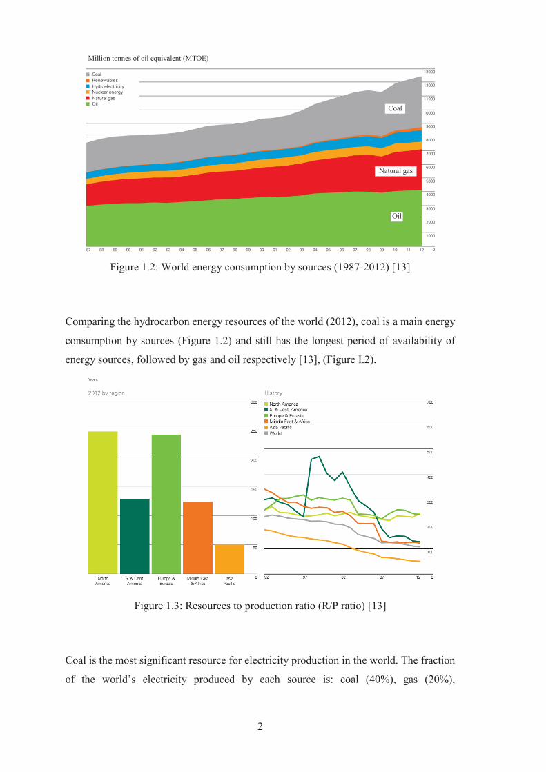
The world’s energy consumption is increasing each year. In 2012, the world’s second
most commonly used energy source was coal, consuming approximately 3,730 MTOE,
compared with oil and gas, which consumed 4,130 and 3,314 MTOE respectively [13].
2
Figure 1.2: World energy consumption by sources (1987-2012) [13]
Comparing the hydrocarbon energy resources of the world (2012), coal is a main energy
consumption by sources (Figure 1.2) and still has the longest period of availability of
energy sources, followed by gas and oil respectively [13], (Figure I.2).
Figure 1.3: Resources to production ratio (R/P ratio) [13]
Coal is the most significant resource for electricity production in the world. The fraction
of the world’s electricity produced by each source is: coal (40%), gas (20%),
Coal
Natural gas
Oil
Million tonnes of oil equivalent (MTOE)

3
hydropower (14%), nuclear (12%), heavy oil and diesel (10%), and renewable energy
(4%) [14], (Figure 1.4).
Figure 1.4: World energy source of electricity [14]
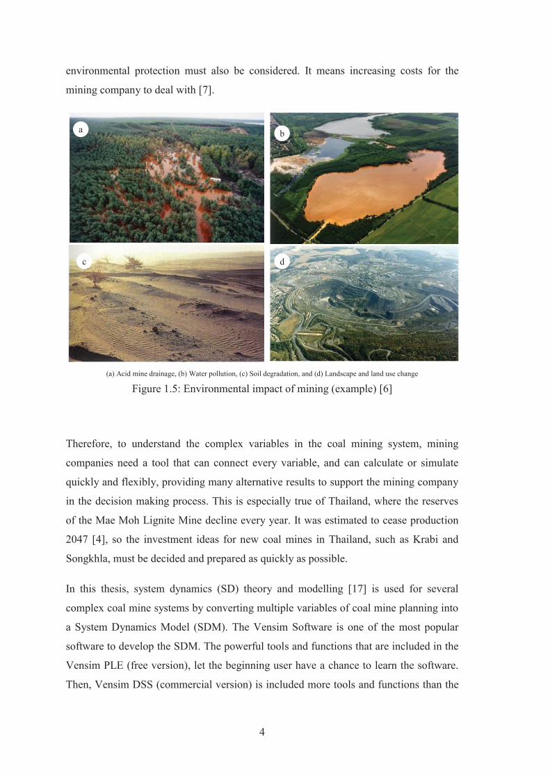
Although current coal mining processes are well managed in some countries by the use
of advanced technologies, some environmental impacts are inevitable to the larger area
and nearby communities; there are also long term effects of the mine closure period.
Possible environmental impacts of mining include; waste water, heavy metal
contamination of water and soil, acid mine drainage, soil degradation, noise, and
vibrations, etc. [15] (Figure 1.5).
Currently, society is concerned about the environmental problems of mining, this means
that mining companies must adhere to stricter rules and try to better control the social
and environmental effects and mine closure management [6, 16]. Therefore, coal
mining companies must more carefully consider investment in a new coal mining
project, than in the past, as there are more associated costs and risks. Moreover, in some
countries, mining companies must provide care and recuperation after the mining
operation, as part of the mine closure period.
The decision to invest in a coal mining project is a complex system and requires a huge
amount of money. Furthermore, it becomes more complicated to decide when the post-
mining period is also included, as mine closure and the activities surrounding social and
40%
20%
12%
10%
14%
4%
Coal
Gas
Nuclear
Heavy Oil & Desel
Hydro
Renewable
Coal
Gas
Hydro
4
environmental protection must also be considered. It means increasing costs for the
mining company to deal with [7].
(a) Acid mine drainage, (b) Water pollution, (c) Soil degradation, and (d) Landscape and land use change
Figure 1.5: Environmental impact of mining (example) [6]
Therefore, to understand the complex variables in the coal mining system, mining
companies need a tool that can connect every variable, and can calculate or simulate
quickly and flexibly, providing many alternative results to support the mining company
in the decision making process. This is especially true of Thailand, where the reserves
of the Mae Moh Lignite Mine decline every year. It was estimated to cease production
2047 [4], so the investment ideas for new coal mines in Thailand, such as Krabi and
Songkhla, must be decided and prepared as quickly as possible.
In this thesis, system dynamics (SD) theory and modelling [17] is used for several
complex coal mine systems by converting multiple variables of coal mine planning into
a System Dynamics Model (SDM). The Vensim Software is one of the most popular
software to develop the SDM. The powerful tools and functions that are included in the
Vensim PLE (free version), let the beginning user have a chance to learn the software.
Then, Vensim DSS (commercial version) is included more tools and functions than the
a b
c d

5
free version, which is needed in this thesis, such as the sensitivity analysis and
optimization tools, is chosen. The Vensim DSS version also included the tool to make a
user interface and package application, which made it comfortable to publish to other
users; the detailed comparisons of the SDM software are shown in the section 2.3 (p.
19). Therefore, propose the development of an application SDM, as a fast and flexible
computer application tool to support the decision making, and to help coal mine
planning. The structure of the model will cover not only the coal mining period, but also
the social and environmental protection, and mine closure. From the results of this
model, possible scenarios with both positive and negative impacts of the coal mining
system can be identified; thus helping the coal mining industry to make the right
decision on their investment. The real data used in the model mainly uses data from the
Mae Moh Lignite Mine and older data from the Krabi Lignite Mine in Thailand for
validating and simulating the alternatives of re-operation of Krabi Lignite Mine in the
future.
1.2 Thailand Coal Mining and Problems
There are 2 general methods of coal mining, (1) surface mining and (2) underground
mining. However, coal mining in Thailand is dominated by surface mining, and the
biggest operational lignite mine in Thailand is the Mae Moh Lignite Mine, (Figure 1.6).
Figure 1.6: Mae Moh Lignite Mine and Power Plant [4]

6
Usually, surface coal mining entails many activities from prospecting, exploration, and
operation, until reclamation after mine closure; thus, it results in a long period for social
and environmental impacts, and needs to be well managed. Nowadays, mines in
Thailand and many countries are required by the government to rehabilitate the mined
area. This means the decision to invest in new coal mines is more complicated and
costly as there are more activities to be managed, and a longer required commitment.
Coal resources are found in many areas from the north to the south of Thailand, most of
them are lignite deposits and small-scale lignite reserves. However, some coal deposits
in Thailand hold more than 100 Mt, and as such can be economically operated,
examples include Mae Moh reserve, Krabi reserve, and Songkhla reserve [5].
Figure 1.7: The simple process of surface coal mining in Thailand (modified) [18]
At the end of 2012, Thailand had proven reserves of about 1,239 Mt, which can be used
for 68 years [13]; and the Mae Moh Lignite Mine is the biggest of these reserves still
running. It has economical reserves of 825 Mt, of which 364 Mt has been used and 461
Mt is still remaining (2011) [4]. All of the produced lignite from the Mae Moh Lignite
Mine is used for electricity generation, producing around 15-17 Mt/y. It is used to feed
7
13 electrical generators that have a total capacity of approximately 2,625 MW, and
cover about 20% of the electricity demand in Thailand [19].
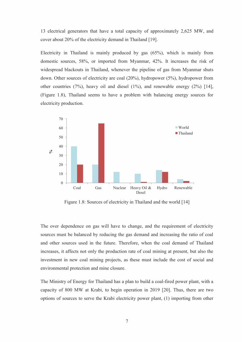
Electricity in Thailand is mainly produced by gas (65%), which is mainly from
domestic sources, 58%, or imported from Myanmar, 42%. It increases the risk of
widespread blackouts in Thailand, whenever the pipeline of gas from Myanmar shuts
down. Other sources of electricity are coal (20%), hydropower (5%), hydropower from
other countries (7%), heavy oil and diesel (1%), and renewable energy (2%) [14],
(Figure 1.8), Thailand seems to have a problem with balancing energy sources for
electricity production.
Figure 1.8: Sources of electricity in Thailand and the world [14]
The over dependence on gas will have to change, and the requirement of electricity
sources must be balanced by reducing the gas demand and increasing the ratio of coal
and other sources used in the future. Therefore, when the coal demand of Thailand
increases, it affects not only the production rate of coal mining at present, but also the
investment in new coal mining projects, as these must include the cost of social and
environmental protection and mine closure.
The Ministry of Energy for Thailand has a plan to build a coal-fired power plant, with a
capacity of 800 MW at Krabi, to begin operation in 2019 [20]. Thus, there are two
options of sources to serve the Krabi electricity power plant, (1) importing from other
0
10
20
30
40
50
60
70
Coal Gas Nuclear Heavy Oil & Desel
Hydro Renewable
%
World Thailand
8
countries, such as Indonesia and Australia etc., or (2) using the domestic lignite
reserves.
Consequently, a tool to support decision-making based upon complex variables, such as
those in coal mining, is very important. This is especially important in Thailand, which
seems to have a problem balancing energy sources, and needs to re-balance by
increasing coal consumption together with other sources in the future. Also, the
domestic coal reserves in Krabi, which could be used for the Krabi Coal Power Plant
Project, should be checked for feasibility and suitability.
1.3 Objectives
This thesis has 2 main objectives. Firstly, to develop a system dynamics model of
surface coal mine planning to act as a decision making tool, to help understand the
behaviour of variables in a surface coal mining system, and to help find the optimum
conditions of a coal project.
Secondly, to use the developed decision making tool for an analysis of the situation of
coal mining in Thailand, especially concerning the possibility of opening a new coal
mine in Krabi to serve the 800 MW Krabi Coal Power Plant Project, and to advise on
the future situation of coal mining in Thailand.
1.4 Remarks
As above mentioned, the importances of coal resources are, firstly as the main energy
source for electricity in the world, and it holds the second place as a source of other
energies [13]. The demand of coal increases every year, despite the limited proven coal
reserves. Therefore, coal reserves have to be managed and sustainability of use planned.
Thailand seems to have a problem balancing energy sources for electricity generation;
gas reserves in Thailand reduce drastically every year due to the high consumption rate,
however Thailand’s coal reserves remain. So, when the decision is made to increase
coal consumption or to invest in new coal mining, all of the advantages and
disadvantages of the mining system should be clear. Then the good management of the
9
coal mining system should start right away from the moment the decision to invest is
made. Hence, in general, the decision support system for coal mine planning is a very
useful tool to provide information and clarify understanding of mining projects; it
enables good decision making, both globally and for the situation in Thailand.
This thesis aims to develop an alternative decision making tool for solving complex
variable problems in coal mine planning. Furthermore, the tool help to understand the
relationship of all relevant variables in the coal mining system. The tool is developed by
using Vensim DSS Software, which is supported by system dynamics theory and
modelling. It is performed and displayed under the various simulated scenarios for
optimizing the most suitable planning conditions for the case study of the Krabi Lignite
Mine Project in Thailand. Successful development of this tool will lead to better
decisions for proper planning and suitable management policy in general coal mining
system and also in the Thai coal mining system.
1.5 Thesis Outlines
The next parts of this thesis are organised into the following chapters:
Chapter 2: the literature reviews, focus on reviewing the problem solving
methodologies and why choose system dynamic modelling to solve this problem. Then
an understanding of system dynamics theory and modelling is made. The software
selection is reviewed and analysed for making a system dynamics model of coal mine
planning, and also the previous research related to decision support systems in mining
or coal mining, are reviewed. Finally, the conclusion of the gap of previous researches
and potential to do this thesis, are included in this chapter.
Chapter 3: the research methodology and model development concentrates on the
system dynamics methodology to develop the system dynamics model of coal mine
planning in this thesis. First, the causal loop diagram of this thesis is made. After that,
the system dynamics model of this thesis is proposed in this chapter.
Chapter 4: the case study Krabi Lignite Mine is proposed, which are the details of coal
mining variables and all other important data of Thailand are collected and analysed to

10
support case study in this thesis. The prototype model is verified by real data of Mae
Moh Lignite Mine. After that, decision criteria and sensitivity analysis conditions, also
the simulation scenario and optimum funding conditions are discussed and selected for
simulating results of case study Krabi Lignite Mine Project.
Chapter 5: The case study simulation results and discussion are proposed. The
modelling and simulation result is made. It is one of the core chapters of the research
which deals with the case study of Krabi Lignite Mine Project, such as result of
sensitivity analysis, the scenario simulation results, the optimum funding results.
Finally, the discussion of the case study which including, scenario simulation
comparison, electricity price effects, economic value of the project and alternatives, are
proposed in this chapter.
Chapter 6: the development of the application interface is presented. The application
software is one of the targets of this thesis. First, the application interface is made.
Then, the application installation and usage are explained in this chapter.
Chapter 7: the summary and recommendation are presented in this chapter. It is a
summary of the big picture of this thesis, and also including some suggestions and ideas
for further research, are provided.
Appendix 1: the background information is covered a general information on coal and
coal mining, and also providing information on Thailand’s coal resources and coal
mining. The information also includes the mining theory, espectically surface mining,
mine planning and coal mining; focusing on understanding of parameters in the coal
mining system and how they are connected. Moreover, the reviewing theories of an
economic analysis and mining cost estimation of the mining project are included.
Appendix 2: additional information tables are presented to support details of parameter
boundary and initial value of variables for all scenarios simulations in this thesis.
Appendix 3: the model equations code is proposed.
Appendix 4: the application code is proposed.
11
2 LITERATURE REVIEWS
A method of solving problems is modelling, which the system under study is replaced
by a simple object. It uses to describe the real system and/or its behavior [94].
Modelling and simulation is commonly used when conducting experiments on a real
system would be impossible or impractical, for example, (1) the high cost of
prototyping and testing, (2) the fragility of the system will not support extensive tests,
and (3) the duration of the experiment in real time is impractical, etc [94].
2.1 Multi-method Simulation Approach
Solving problems by modelling are based on abstraction, simplification, quantification,
and analysis. Each of the different modelling methodologies assumes different levels of
each of these factors [93].
Nowadays, there are 3 modelling methodologies used to solve problems, including, (1)
System Dynamics (SD) modelling, (2) Discrete Event (DE) modelling, and (3) Agent
Based (AB) modelling. The first two methodologies were developed by Jay Forrester in
1950s, and by Geoffrey Gordon in 1960s, respectively. Both methods employ a top-
down view of things. Finally, the AB approach, a more recent development, is a
bottom-up approach where the modeler focuses on the behavior of the individual
objects [93].
The SD method assumes a high abstraction level, a big picture level, and is primarily
used for strategic/policy level problems. While the DE model is commonly used for
operational and tactical levels, and AB model is flexibly used at all levels, such as
competing companies, consumers, projects, ideas, vehicles, pedestrians, or robots. The
methodology modelling selection is shown below [93].
When a system is individual data, then use an AB approach.
When a system is complex continuous variables, then use an SD approach.
When a system can be described as a process, then use a DE approach.
12
Therefore, whenever the system or problem is complex variables and continuous
changing along the time, SD approach is probably be a first choice to solve the problem.
2.2 System Dynamics Theory and Modelling
2.2.1 Overview
System dynamics is an academic discipline created by Prof. Jay W. Forrester of the
Massachusetts Institute of Technology (MIT). System dynamics is originally rooted in
the management and engineering sciences, but has gradually developed into a tool
useful in the analysis of social, economic, physical, chemical, biological, and ecological
systems [55].
System Dynamics [17] is generally used in the field of social science, business,
management, economic, and environment [56, 57]. Then, Meadow et al., Is the first
team to publish the well-known books that referred to the system dynamics theory by
name “Limit to Growth” (1972), “Beyond the Limit” (1993), and “Limits to Growth:
The 30-Year Update” (2004) [58]. Even now, the system dynamics theory is applied to
use in many fields of research.
System dynamics is a computer-aided approach to policy analysis and design. It applies
to dynamic problems arising in complex social, managerial, economic, or ecological
systems – literally any dynamic systems characterised by interdependence, mutual
interaction, information feedback, and circular causality [59].
The field developed initially from the work of Jay W. Forrester [57]. His seminal book
Industrial Dynamics (Forrester, 1961) is still a significant statement of philosophy and
methodology in the field. Within 10 years of its publication, the span of applications
grew from corporate and industrial problems to include the management of research and
development, urban stagnation and decay, commodity cycles, and the dynamics of
growth in a finite world. It is now applied in economics, public policy, environmental
studies, and theory building in social science, and other areas, as well as its home field,
management. The name industrial dynamics no longer does justice to the breadth of the
field, so it has become generalised to system dynamics. The modern name suggests
links to other systems methodologies, but the links are weak and misleading. System

13
dynamics emerge out of servomechanisms engineering, not general systems theory or
cybernetics (Richardson, 1991) [59].
2.2.2 The System Dynamics Approach
In the field of system dynamics, a system is defined as a collection of elements that
continually interact over time to form a unified whole. The underlying relationships and
connections between the components of a system are called the structure of the system.
One familiar example of a system is an ecosystem. The structure of an ecosystem is
defined by the interactions between animal populations, birth and death rates, quantities
of food, and other variables specific to a particular ecosystem. The structure of the
ecosystem includes the variables important in influencing the system [55].
The term dynamics refers to change over time. If something is dynamic, it is constantly
changing. A dynamic system is therefore a system in which the variables interact to
stimulate changes over time. System dynamics is a methodology used to understand
how systems change over time. The way in which the elements or variables composing
a system vary over time is referred as the behaviour of the system. In the ecosystem
example, the behaviour is described by the dynamics of population growth and decline.
The behaviour is due to the influences of food supply, predators, and environment,
which are all elements of the system [55].
One feature that is common to all systems is that a system’s structure determines the
system’s behaviour. System dynamics links the behaviour of a system to its underlying
structure. System dynamics can be used to analyse how the structure of a physical,
biological, or literary system can lead to the behaviour that the system exhibits. By
defining the structure of an ecosystem, it is possible to use system dynamics analysis to
trace out the behaviour over time of the ecosystem based upon its structure [55].
The system dynamics approach involves [59]:
Defining problems dynamically, in terms of graphs over time.
Striving for an endogenous, behavioural view of the significant dynamics of a
system, a focus inward on the characteristics of a system that themselves
generate or exacerbate the perceived problem.

14
Thinking of all concepts in the real system as continuous quantities
interconnected in loops of information feedback and circular causality.
Identifying independent stocks or accumulations (Levels or Stock) in the system
and their inflows and outflows (Rates or Flow).
Formulating a behavioural model capable of reproducing, by itself, the dynamic
problem of concern. The model is usually a computer simulation model
expressed in nonlinear equations, but is occasionally left un-quantified as a
diagram capturing the stock-and-flow/causal feedback structure of the system.
Deriving understandings and applicable policy insights from the resulting
model.
Implementing changes resulting from model-based understandings and insights.
2.2.3 SD Modelling and Simulation
Mathematically, the basic structure of a formal system dynamics computer simulation
model is a system of coupled, nonlinear, first-order differential equations or integral
equations, [59]
ddt
X t =f(X, P) (2.1)
where X is a vector of levels (stocks or state variables),
P is a set of parameters,
f is a nonlinear vector-valued function.
Simulation of such systems is easily accomplished by partitioning simulated time into
discrete intervals of length, (dt), and stepping the system through time, one (dt) at a
time. Each state variable is computed from its previous value and its net rate of change
x' t : x t =x(t-dt)+dt×x'(t-dt). In the earliest simulation language in the field
(DYNAMO), this equation is written with time scripts, K is the current moment, J is the
previous moment, and JK is the interval between time J and K:
X.K=X.J+[(dt)×(X_rate.JK)], (Richardson and Pugh, 1981). The computation interval
“dt” is selected small enough to have no discernible effect on the patterns of dynamic
behaviour exhibited by the model. In more recent simulation environments, more
15
sophisticated integration schemes are available (although the equation written by the
user may look like this simple Euler integration scheme), and time scripts may not be
evidenced.
Forrester's original work stressed a continuous approach, but increasingly modern
applications of system dynamics contain a mix of discrete differential equations and
continuous differential or integral equations. Some users associated with the field of
system dynamics work on the mathematics of such structures, study the theory and
mechanics of computer simulation, analysis, and simplification of dynamic systems,
policy optimization, dynamical systems theory, and complex nonlinear dynamics and
deterministic chaos.
The main applied work in the field, however, focuses on understanding the dynamics of
complex systems for the purpose of policy analysis and design. The conceptual tools
and concepts of the field – including feedback thinking, stocks and flows, the concept of
feedback loop dominance, and an endogenous point of view – are as important to the
field as its simulation methods.
2.2.4 Feedback Thinking
Conceptually, the feedback concept is at the heart of the system dynamics approach.
Diagrams of loops of information feedback and circular causality are tools for
conceptualising the structure of a complex system and for communicating model-based
insights. Intuitively, a feedback loop exists when information resulting from some
action travels through a system and eventually returns in some form to its point of
origin, potentially influencing future action. If the tendency in the loop is to reinforce
the initial action, the loop is called a positive or reinforcing feedback loop; if the
tendency is to oppose the initial action, the loop is called a negative or balancing
feedback loop. The sign of the loop is called its polarity. Balancing loops can be
variously characterised as goal-seeking, equilibrating, or stabilising processes. They can
sometimes generate oscillations, as when a pendulum seeking its equilibrium goal
gathers momentum and overshoots it. Reinforcing loops are sources of growth or the
accelerating collapse; they are disequilibrating and destabilizing. Combined, reinforcing
16
and balancing circular causal feedback processes can generate all manner of dynamic
patterns [59].
Loop dominance and nonlinearity
The loop concept underlying feedback and circular causality by itself is not enough.
However, the explanatory power and insights of feedback understandings also rest on
the notions of active structure and loop dominance. Complex systems change over time.
A crucial requirement for a powerful view of a dynamic system is the ability of a mental
or formal model to change the strengths of influences as conditions change, that is to
say, the ability to shift the active or dominant structure [59].
In a system of equations, this ability to shift-loop dominance comes about endogenously
from nonlinearities in the system. For example, the S-shaped dynamic behaviour of the
classic logistic growth model can be seen as the consequence of a shift in
loop dominance from a positive, self-reinforcing feedback loop (aP) producing
exponential-like growth to a negative balancing feedback loop (-bP2) that brings the
system to its eventual goal. Only nonlinear models can endogenously alter their active
or dominant structure and shift loop dominance. From a feedback perspective, the
ability of nonlinearities to generate shifts in loop dominance and capture the shifting
nature of reality is the fundamental reason for advocating nonlinear models of social
system behaviour [59].
The endogenous point of view
The concept of endogenous change is fundamental to the system dynamics approach. It
dictates aspects of model formulation: exogenous disturbances are seen at most as
triggers of system behaviour, like displacing a pendulum; the causes are contained
within the structure of the system itself like the interaction of a pendulum’s position and
momentum that produces oscillations. Correct responses are also not modelled as
17
functions of time, but are dependent on conditions within the system. Time by itself is
not seen as a cause [59].
More importantly, theory building and policy analysis are significantly affected by this
endogenous perspective. Taking an endogenous view exposes the natural compensating
tendencies in social systems that conspire to defeat many policy initiatives. Feedback
and circular causality are delayed, devious, and deceptive. For understanding, system
dynamics practitioners strive for an endogenous point of view. The effort is to uncover
the sources of system behaviour that exist within the structure of the system itself [59].
2.2.5 System Structure
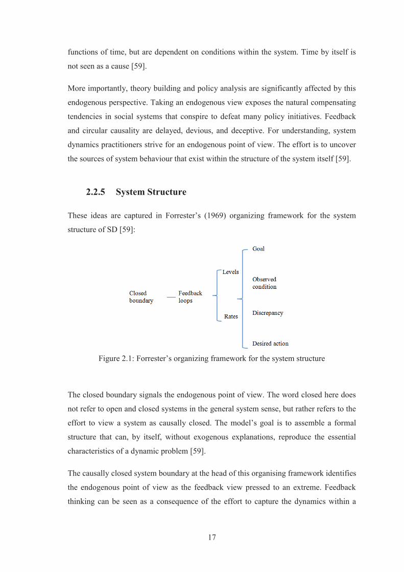
These ideas are captured in Forrester’s (1969) organizing framework for the system
structure of SD [59]:
Figure 2.1: Forrester’s organizing framework for the system structure
The closed boundary signals the endogenous point of view. The word closed here does
not refer to open and closed systems in the general system sense, but rather refers to the
effort to view a system as causally closed. The model’s goal is to assemble a formal
structure that can, by itself, without exogenous explanations, reproduce the essential
characteristics of a dynamic problem [59].
The causally closed system boundary at the head of this organising framework identifies
the endogenous point of view as the feedback view pressed to an extreme. Feedback
thinking can be seen as a consequence of the effort to capture the dynamics within a

18
closed causal boundary. Without causal loops, all variables must trace the sources of
their variation ultimately outside a system. Assuming instead that the causes of all
significant behaviour in the system are contained within some closed causal boundary
forces causal influences to feed back upon themselves, forming causal loops. Feedback
loops enable the endogenous point of view and give it structure [59].
Levels and rates
Stocks (levels) and the flows (rates) that affect other parameters are essential
components of system structure. A map of causal influences and feedback loops is not
sufficient to determine the dynamic behaviour of a system. A constant inflow yields a
linearly rising stock; a linearly rising inflow yields a stock rising along a parabolic path,
and so on. Stocks (accumulations, state variables) are the memory of a dynamic system
and are the sources of its disequilibrium and dynamic behaviour [59].
J. W. Forrester (1961) placed the operating policies of a system among its rates (flows),
many of which assume the classic structure of a balancing feedback loop striving to take
action to reduce the discrepancy between the observed condition of the system and a
goal. The simplest rate structure results in an equation of the form [59]:
Netflow=(Goal-Stock)
ADJTIM (2.2)
where ADJTIM is the period of time over which the level adjusts to reach the goal [59].
Behaviour is a consequence of system structure
The importance of levels and rates appears clearer, when one takes a continuous view of
structure and dynamics. Although a discrete view, focusing on separate events and
decisions, is entirely compatible with an endogenous feedback perspective, the system
dynamics approach emphasises a continuous view. The continuous view strives to look
beyond events to see the dynamic patterns underlying them. Moreover, the continuous
view focuses not on discrete decisions, but on the policy structure underlying decisions.
19
Events and decisions are seen as surface phenomena that ride on an underlying tide of
system structure and behaviour. It is that the underlying tide of policy structure and
continuous behaviour that is the system dynamicity’s focus [59].
There is thus a distancing inherent in the system dynamics approach – not so close as to
be confused with discrete decisions and myriad operational details, but not so far away
as to miss the critical elements of policy structure and behaviour. Events are
deliberately blurred into dynamic behaviour. Decisions are deliberately blurred into
perceived policy structures. Insights into the connections between system structure and
dynamic behaviour, which are the goal of the system dynamics approach, come from
this particular perspective of distance [59].
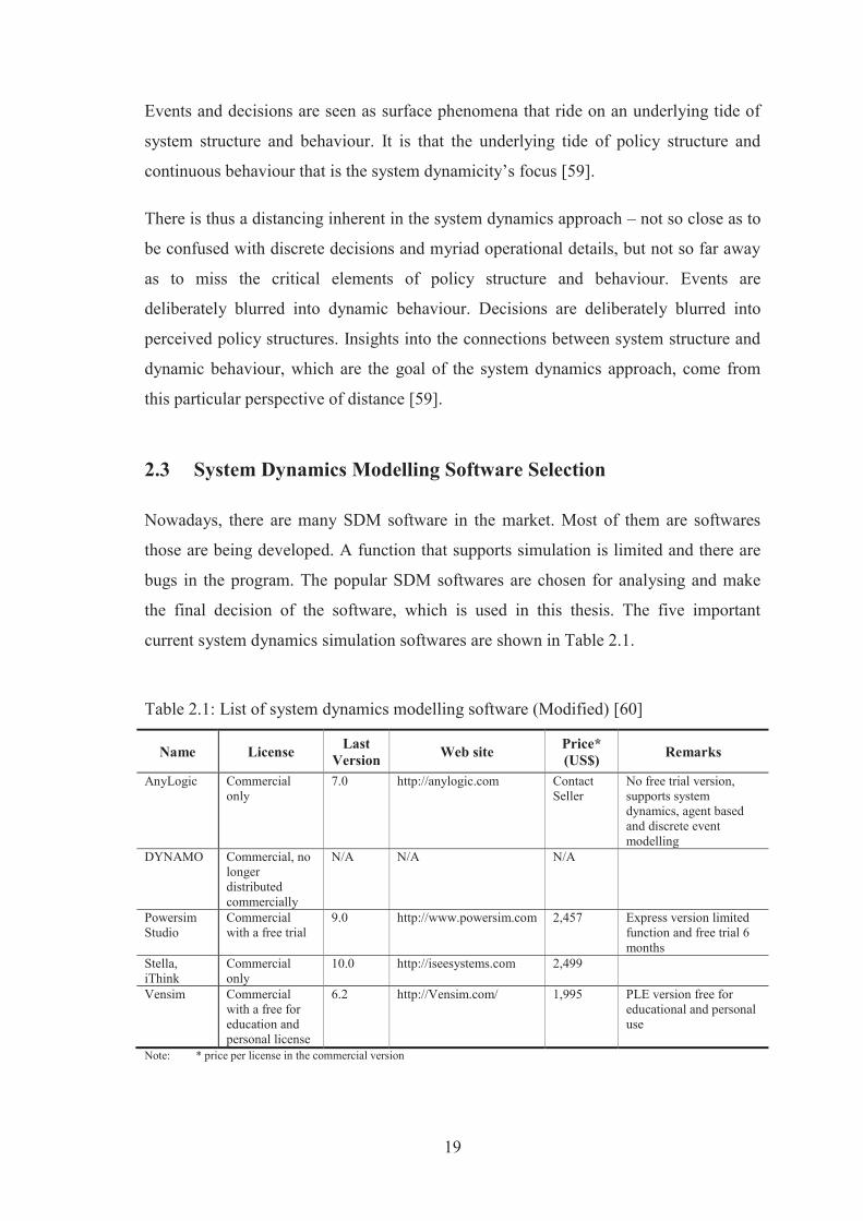
2.3 System Dynamics Modelling Software Selection
Nowadays, there are many SDM software in the market. Most of them are softwares
those are being developed. A function that supports simulation is limited and there are
bugs in the program. The popular SDM softwares are chosen for analysing and make
the final decision of the software, which is used in this thesis. The five important
current system dynamics simulation softwares are shown in Table 2.1.
Table 2.1: List of system dynamics modelling software (Modified) [60]
Name License Last Version Web site Price*
(US$) Remarks
AnyLogic Commercial only
7.0 http://anylogic.com Contact Seller
No free trial version, supports system dynamics, agent based and discrete event modelling
DYNAMO Commercial, no longer distributed commercially
N/A N/A N/A
Powersim Studio
Commercial with a free trial
9.0 http://www.powersim.com 2,457 Express version limited function and free trial 6 months
Stella, iThink
Commercial only
10.0 http://iseesystems.com 2,499
Vensim Commercial with a free for education and personal license
6.2 http://Vensim.com/ 1,995 PLE version free for educational and personal use
Note: * price per license in the commercial version
20
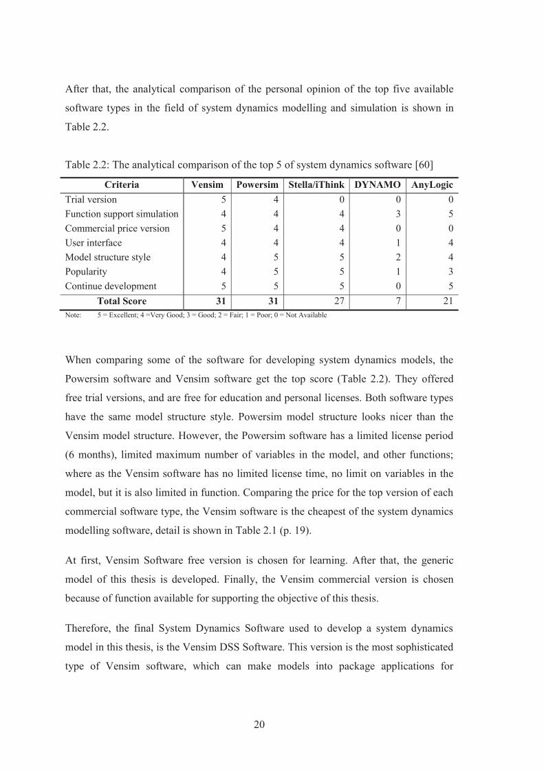
After that, the analytical comparison of the personal opinion of the top five available
software types in the field of system dynamics modelling and simulation is shown in
Table 2.2.
Table 2.2: The analytical comparison of the top 5 of system dynamics software [60]
Criteria Vensim Powersim Stella/iThink DYNAMO AnyLogic Trial version 5 4 0 0 0 Function support simulation 4 4 4 3 5 Commercial price version 5 4 4 0 0 User interface 4 4 4 1 4 Model structure style 4 5 5 2 4 Popularity 4 5 5 1 3 Continue development 5 5 5 0 5
Total Score 31 31 27 7 21 Note: 5 = Excellent; 4 =Very Good; 3 = Good; 2 = Fair; 1 = Poor; 0 = Not Available
When comparing some of the software for developing system dynamics models, the
Powersim software and Vensim software get the top score (Table 2.2). They offered
free trial versions, and are free for education and personal licenses. Both software types
have the same model structure style. Powersim model structure looks nicer than the
Vensim model structure. However, the Powersim software has a limited license period
(6 months), limited maximum number of variables in the model, and other functions;
where as the Vensim software has no limited license time, no limit on variables in the
model, but it is also limited in function. Comparing the price for the top version of each
commercial software type, the Vensim software is the cheapest of the system dynamics
modelling software, detail is shown in Table 2.1 (p. 19).
At first, Vensim Software free version is chosen for learning. After that, the generic
model of this thesis is developed. Finally, the Vensim commercial version is chosen
because of function available for supporting the objective of this thesis.
Therefore, the final System Dynamics Software used to develop a system dynamics
model in this thesis, is the Vensim DSS Software. This version is the most sophisticated
type of Vensim software, which can make models into package applications for

21
publishing to other users. The details of how to use the Vensim can be found in the
Vensim User Manual [87].
2.4 System Dynamics Model and Decision Making in Mining
System dynamics theory, modelling, and the development of a decision making tool has
been applied in the field of mining for a long time. Focusing on mining and coal mining
fields, some researchers have used this conceptual theory to solve their problems in the
mining fields. This is discussed in this section:
It began with Budzik, et.al., (1976) [61] developing an energy model, called FOSSIL1,
by using the system dynamics theory. The purpose of the development was to
understand energy balancing, to manage the USA reserves of coal, oil, and gas. Later,
model updates of FOSSIL2 and FOSSIL3, etc., were published.
C. Roumpos, et.al., (2004) proposed the development of a decision making model for
lignite deposit exploitability. The model was developed in the form of mathematical
equations modelling, which included parameters in four sub models, (1) the deposit
condition and the mine characteristics, (2) environmental and socioeconomic
parameters, (3) competition, and (4) market [7]. The conceptual model of C. Roumpos,
et.al., is shown in Figure 2.2.
Figure 2.2: The conceptual model of C. Roumpos, et.al. [7]

22
The C. Roumpos mathematical model result of annual cash flow (Ai) in € is shown in
equation (2.3) [7]:
(2.3)
Where, Pα = Capacity of the power plant (MW), Tα = Operating hour of the power plant (h/y),
Iα = Investment cost for power plant construction (€), Hα = Calorific Value (kcal/m3),
cpα = Production cost in power plant (€/kWh), ceα = Environmental cost (€/t), cf = Fuel
cost (€/m3), k = Construction time (y), N = Depreciation time or project life time (y),
pα = Selling price of electricity (€/kWh), n = Power plant efficiency (%), ε = Discount
rate (%), and t = Tax rate (%).
Fan, et al. (2007) developed a system dynamics base model for coal investment in
China. In this paper, a system dynamics model was developed taking the investment in
the coal industry, available reserves, mine construction and coal supply capability into
account [62].
Figure 2.3: Fan’s flow diagram of coal production and supply [62]
PCsmNPCsm SPCsm
Cmc
MERS
ARS
ICGP
GPI
NARS
MRSERsm
MERsm
Psm
CD
ERtvMERtv
Ptv
Ism
ICmw
ERS

23
where: ARS Available reserves for constructing mines MERsm Mining-employed reserves by stale-owned mines CD Coal demand MRS Mining reserves Cmc Coefficient of mine construction MERtv Mining-employed reserves by town or village mines ERS Explored reserves NARS New available reserves for mine construction ERsm Extraction in state-owned mines NPCsm New production capacity of state-owned mines ERtv Extraction in town or village owned mines PCcm Production capacity of constructing mines GPI Geological prospecting investment PCnsp Production capacity of newly started project ICGP Investment coefficient in geological prospecting PCsm Production capacity of state-owned mines ICmw Investment coefficient of mining and washing of coal Psm Production of state-owned mine Ism Investment in state-owned mine construction Ptv Production of town or village owned mines MERS Mining-employed reserves SPCsm Scrapped production capacity of state-owned mines
The results of Fan’s research showed many scenarios. The simulation of the model
helped to find the economic scenario, where the available reserves would approximately
reach 8.6 Bt/y, to meet the requirements of China’s expectation.
Caselles-Moncho, et al. (2006) studied the dynamic simulation model of a coal thermo-
electric plant with a flue gas desulphurization system (FGD). This research developed a
dynamic simulation model that had been used to present the likely responses of the
electricity industries’ latest perturbations such as changes in environmental regulations,
international fuel market evolution, restriction on fuel supply and increase on fuel
prices, liberalisation of the European Electricity Market, and the results of applying
energy policies and official tools such as taxes and emission allowances [63].
Figure 2.4: Concept of the Caselles-Moncho’s model [63]
24
The results of Caselles-Moncho’s research showed the optimal strategy, including: (a)
minimum energy production (b) specific net consumption of 2,207,000 t/GWh (the
consumption curve means), (c) theoretical participation of the different fuels, (d)
desulphurization running at 100% and (e) minimum commercialization of ashes, scoria,
and gypsum [63].
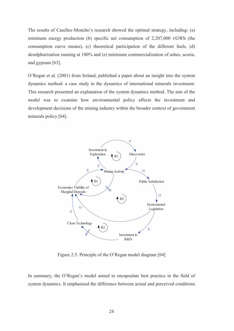
O’Regan et al. (2001) from Ireland, published a paper about an insight into the system
dynamics method: a case study in the dynamics of international minerals investment.
This research presented an explanation of the system dynamics method. The aim of the
model was to examine how environmental policy affects the investment and
development decisions of the mining industry within the broader context of government
minerals policy [64].
Figure 2.5: Principle of the O’Regan model diagram [64]
In summary, the O’Regan’s model aimed to encapsulate best practice in the field of
system dynamics. It emphasised the difference between actual and perceived conditions
Investment inExploration Discoveries
Mining Activity
Economics Viability ofMarginal Deposits
Clean Technology
Investment inR&D
EnviromentalLegislation
Public Satisfaction
S
S
S
S
O
S
SS
O
O
O
R1
B1
B2
R2

25
as a basis for action. It made explicit the underlying assumptions as a basis for further
expansion. It highlighted system structure as a catalyst for change. It did not by itself
provide objective answers. Instead, it was a learning device and an aid to understanding.
It was not a replacement for analytical thinking, but rather complementary to it [64].
Therefore, the decision support system of coal mine planning by using system dynamics
model is a new and efficient tool to support making a decision on complex variables of
new coal mining project. It can be fulfilled objectives of this thesis, which included the
additional cost of social and environmental protection cost and mine closure cost.
The system dynamics modelling is the most suitable methodology in this purposed
because it can deal with:
complex relationship of variables,
flexibility of changing value of input variables,
fast and no limit of calculation in a long period of mining project, and
easy to find sensitivity of variables and optimum solutions.
After reviewed and analysed, Vensim DSS software is chosen to develop the model
because it has a free version for beginner to learn and the commercial version covers all
functions that need to use in this thesis. Finally, it is also be the cheapest one of the
popular software in this field.
2.5 Chapter Conclusion
The literature review of this thesis starts with the background information in Appendix
1 (p. 124), and it gives ideas to develop this thesis.
The mining cost estimation technique by O'Hara (1980), referred to in Hustrulid, et.al,
(1998, 2006) [43, 44] is mainly used in this thesis. This technique is also used or
developed in many other works. It proposed the mining cost estimation in the form of
the mathematical equations. The O'Hara cost estimation covers (1) capital cost, (2)
general and administrative cost, and (3) operating cost. However, it does not cover
26
prospecting and exploration cost, mine closure cost, and also a part of social and
environmental protection cost. The use of O’Hara’s cost estimation, which is mainly
used for mining cost estimation in this thesis, is also confirmed in initial mining projects
by M. Osanloo, et.al. (2004) [86]. It is noticed that the O’Hara’s technique normally
gave a higher estimated result when compared with the real result.
The economic decision in business, especially in mining, still popularly uses multiple
criteria like Net Cash Flow (NCF), Net Present Value (NPV), Internal Rate of Return
(IRR), Payback Period (PP), Cash Flow Analysis (CFA), etc [9-10, 51, 79, 85].
Furthermore, NPV is a main criterion for decision making on investment and project
planning. Therefore, the “NPV Balance” is the summation of the mining fund and NPV,
and is the final economic criteria for accepting or rejecting a coal mining project.
The review of the literature also found some research in mining and coal mining that
used the concept and theory of system dynamics, such as Caselles-Moncho, et.al.’s
research (2006) [63], which used economic decision criteria as Cash Flow Analysis
(CFA) and developed a system dynamics model of coal-gas power plant management in
Spain. Moreover, the research of Fan, et.al. (2007) [62], also developed a system
dynamics model of coal mining investment in China, which looked for suitable strategy
and policy control of coal mining in China.
Furthermore, some research focused on the decision making tool in lignite deposit like
C. Roumpos (2004) [7], which also gave the idea and some important parameters for
developing the SDM of this thesis. The idea of social and environmental protection and
post-mining management and evaluation should be the responsibility of a mining
company, is shared by many researchers, such as C. Drebenstedt, et.al. (2004, 2006,
2010, and 2011) [6, 16, 40, 53-54], L. Wilde (2007) [46], A. H. Watson (2006) [45],
and A. Peralta-Romero and K. Dagdelen (2007) [47], etc. This literature review also
proposed the idea that environmental protection costs are always cheaper than the costs
associated with the correction of environmental problem when they arise.
Therefore, the gap in previous researches can be filled by the development of system
dynamics model as a decision support system of coal mine planning in this thesis.
27
3 RESEARCH METHODOLOGY AND MODEL DEVELOPMENT
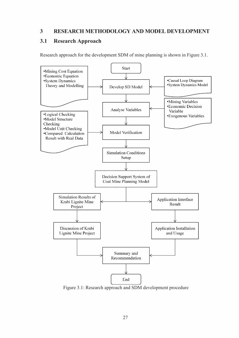
3.1 Research Approach
Research approach for the development SDM of mine planning is shown in Figure 3.1.
Figure 3.1: Research approach and SDM development procedure
28
Research approach starts with the development of SD model. The boundary of this SD
model development is supported by mining cost equations, economic equations, and
others, which explained in Appendix 1: Background Information (p. 124). The system
dynamics theory and modelling and Vensim Software (Chapter 2) are used to develop
SDM of coal mine planning. First, the causal loop diagram, and then system dynamics
model, are developed in this part, see details in Section 3.2.1 and Section 3.2.2.
After the prototype model is made, the step of analyse variables in the case study of
Krabi Lignite Mine is made, see details in Chapter 4 (p. 46). The variables are separated
into 3 groups, (1) mining variables (p. 46), (2) economic decision variables (p. 51), and
(3) exogenous variables (p. 52).
After that, the model is verified in 4 steps, including, (1) logical checking (p. 60), (2)
model structure checking (p. 60), (3) model unit checking (p. 61), and (4) compared
calculation result with real data (p. 61). When the model passed step of model
verification, it goes to the simulation conditions setup (p. 66). After that, the decision
support system of coal mine planning model is used to simulate the case study result,
see in chapter 5 (p. 70) and develop the application interface, see chapter 6 (p. 105).
The simulation results of Krabi Lignite Mine Project are included, (1) sensitivity
analysis results (p. 70), (2) scenario simulation results (p. 81), and (3) optimum funding
result (p. 91). Then, it comes to the discussion of Krabi Lignite Mine Project in the big
picture with Krabi Coal Power Plant is shown in Section 5.2 (p. 94).
Moreover, to support general end users, the application interface for the model is
developed. It helps much to reduce the confusing how to use the model. The application
interface result is shown in Section 6.1 (p. 106), and then the application installation
and usage is done, see in Section 6.2 (p. 114).
Finally, the summary of this research and recommendation for future research
development is proposed in Chapter 7 (p. 116).
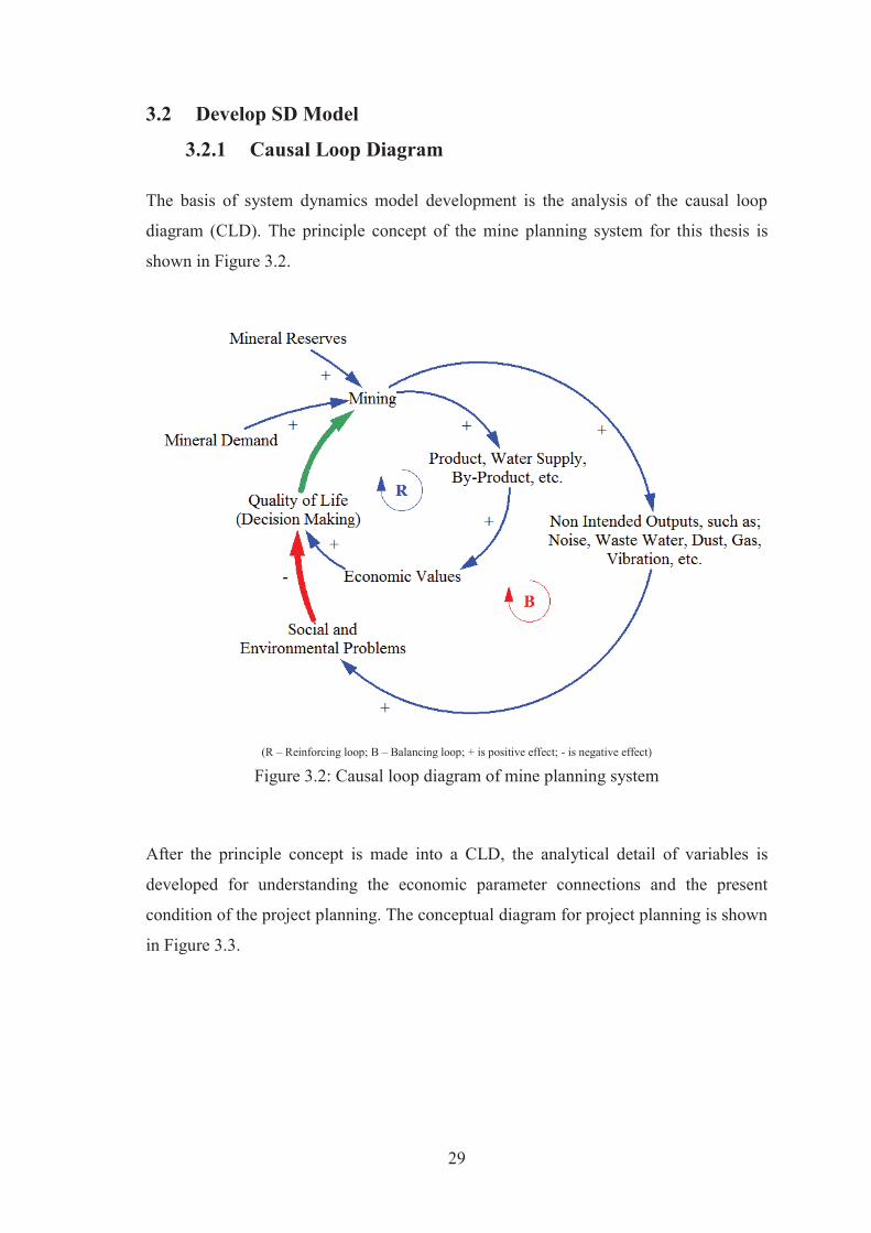
29
3.2 Develop SD Model
3.2.1 Causal Loop Diagram
The basis of system dynamics model development is the analysis of the causal loop
diagram (CLD). The principle concept of the mine planning system for this thesis is
shown in Figure 3.2.
(R – Reinforcing loop; B – Balancing loop; + is positive effect; - is negative effect)
Figure 3.2: Causal loop diagram of mine planning system
After the principle concept is made into a CLD, the analytical detail of variables is
developed for understanding the economic parameter connections and the present
condition of the project planning. The conceptual diagram for project planning is shown
in Figure 3.3.

30
Figure 3.3: The conceptual diagram for mine planning decision (Narrow Sense)
Because of the recent importance placed on social and environmental problems caused
by mining and mine closure, the newly modified conceptual diagram (Wider Sense) for
mine planning is made, (Figure 3.4).
The concept of social and environmental protection (S&EP) cost could be anything to
protect the community nearby mining from effects of mine, which are affected directly.
In addition, it should make the better quality of life of the community, such as, health
care insurance, scholarships, public infrastructure, etc. The mine closure cost is also
important because after the end of mine operation many mining tries to stop every
activity and do not have mine closure period because it is costly without income.
Therefore, a solution which would be a key to sustainability of mining and social and
community nearby is mining fund. The mining fund should be managed by the
committee, which including mining company, community, government, etc. It is a
better guarantee to protect the environment and quality of life after the end of mining,
the conceptual diagram for mine planning decision (Widest Sense), (Figure 3.5).
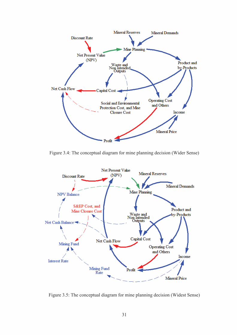
31
Figure 3.4: The conceptual diagram for mine planning decision (Wider Sense)
Figure 3.5: The conceptual diagram for mine planning decision (Widest Sense)
32
3.2.2 System Dynamics Model
Boundary of Parameters in the Model Development
Parameters in the model can be arranged in many ways as mentioned in the section
2.2.5 (p. 17), but in this case, the parameters are arranged into two groups:
Input parameters
The input parameters are, in other words, exogenous parameters. These parameters are
not influenced by any other parameters in the model, but are controlled by the source of
data and information outside of the model boundary. The user can change the value of
each input parameter freely, to see the effect of the output parameters. The input
parameters can be divided into two groups, (1) the main input parameters and (2) the
auxiliary input parameters.
There are 48 main input parameters. There are highlighted in the bold text style for
some important input parameters, which are used to simulate scenarios in the model.
The list of the input parameters is shown on the Table II.4 (p. 169).
Generally, the auxiliary input parameters, of which there are two groups, support model
calculation. The first group is the unit converter; these do not have to change value
because the value is specific for converting units. The list of auxiliary input parameters
for unit conversion is shown on the Table II.5 (p. 169).
The second group of the auxiliary input parameters is the group for unit cost estimation
(k.xi) and the powers for the pattern graph (n.xi), which have a certain number of values
from the theory of cost estimation by O'Hara (1980) [43, 44]. However, the value of
these auxiliary input parameters can be adjusted, if the users know the unit cost specific
to their own mine. A list of auxiliary input parameters for the unit cost estimation (k.xi)
and the powers for the pattern graph (n.xi) is shown on the Table II.6 (p. 170).
33
Output parameters
The output parameters are endogenous parameters. These parameters are always
influenced by others parameters in the model, or in some cases by the end point
parameter of the model. There are 138 output parameters that are calculated by the
model. The main output parameters are highlighted in the bold text style. The list of
output parameters is shown on the Table II.7 (p. 170).
SD Model Structure
Introduction
The developed result of the system dynamics model structure of the decision support
system of coal mine planning can be separated into six sub-model including:
Mining System
Economic Decision
Total Cost and Worker Estimation
Operating Cost Estimation
Capital Cost Estimation
Power Plant Economic Value
All sub-models are connected by other parameters such as, mining production rate,
operating cost, and capital cost, etc. The SDM equations are shown in Appendix 3:
Model Equations Code (p. 173).
Model structure of mining system
The mining system sub-model structure began with the stock or amount of coal
reserves; this may refer to potential reserves or economical reserves from the geological
analysis of the ore body. In this development, the coal production rate directly affected
the coal reserves, causing them to reduce, and is controlled by the demand of electricity
consumption and the capacity of the coal-fired power plant. This model structure
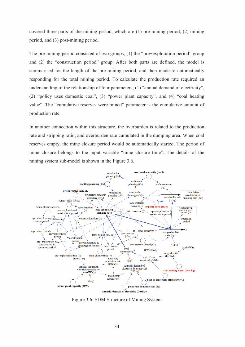
34
covered three parts of the mining period, which are (1) pre-mining period, (2) mining
period, and (3) post-mining period.
The pre-mining period consisted of two groups, (1) the “pre+exploration period” group
and (2) the “construction period” group. After both parts are defined, the model is
summarised for the length of the pre-mining period, and then made to automatically
responding for the total mining period. To calculate the production rate required an
understanding of the relationship of four parameters; (1) “annual demand of electricity”,
(2) “policy uses domestic coal”, (3) “power plant capacity”, and (4) “coal heating
value”. The “cumulative reserves were mined” parameter is the cumulative amount of
production rate.
In another connection within this structure, the overburden is related to the production
rate and stripping ratio; and overburden rate cumulated in the dumping area. When coal
reserves empty, the mine closure period would be automatically started. The period of
mine closure belongs to the input variable “mine closure time”. The details of the
mining system sub-model is shown in the Figure 3.6.
Figure 3.6: SDM Structure of Mining System
35
Model structure of economic decision
The economic decision sub-model structure starts with the connection of production
rate from the mining system sub-model, and the cost estimation sub-model, which
included the capital cost estimation and the operating cost estimation.
The unit cost estimations, which are estimated by the model, were multiplied by the
production rate to provide cost of the mining project. The capital cost is controlled by
the pre-mining period, which is the main time for investment in the project outside of
re-investment in the “equipment life cycle”.
The operating cost is controlled by the mining period, which is the main part earning
revenue. Generally, “gross revenue” is a function of coal production rate and prices of
coal, from which the “royalties rate” is removed to become “net revenue”. Then, the
“operating cost” is removed from the net revenue. In this thesis, the additional part of
the “mining fund cost” is cut from the cash flow of the company when the mining
company made a profit, and it is deposited in the bank, this extra stock is referred to as
the “mining fund”. The mining fund has two purposes; (1) for social and environmental
protection cost, to be used in the mine operation period, and (2) for mine closure costs,
which would be used in the post-mining period.
The “gross profit” had the “non-cash deduction” cut from it, which included the
“depreciation” and “depletion”. After that, the gross profit became “taxable income” for
calculating the corporation tax with the tax rate. Then, the “net profit” is calculated by
cutting the corporate tax and adding the non-cash deduction value; thus generating
“cash flow after tax”. The cash flow after tax is used to calculate the “Net Cash Flow”
and the “Net Present Value”.
Finally, the Net Cash Flow and the Net Present Value are balanced with the mining
fund, in the “Net Cash Balance” and the “NPV Balance” respectively, to check the
money status for supporting the social and environmental protection costs, and mine
closure costs. Detail is shown in Figure 3.7.

36
Figure 3.7: SDM Structure of Economic Decision
Model structure of total cost and worker estimation
The total costs, the amount of workers, and production rate of mining, which connect
from the structure of the mining system sub-model and the model of cost estimation,
can be estimated. Detail is shown in Figure 3.8.
The “total mining cost estimation” comprised two main parts, (1) capital cost estimation
and (2) operating cost estimation. The “total number of people in mine” is estimated
from three groups including; (1) the “number of mine personnel”, (2) the “number of
service personnel”, and (3) the “number of administrative and technical personnel”,
which are the function of “production planning” and “overburden planning”.

37
Figure 3.8: SDM Structure of Total Cost and Worker Estimation
Model structure of operating cost estimation
The operating cost estimation sub-model is the final part of the model structure group.
This part also connects with other parts of the model by the “total materials mined”,
“coal passed the primary crusher”, and others. The “operating costs” generally consists
of two parts, (1) the “total daily operating costs”, and (2) the “other operating costs”.
The theory of total daily operating costs includes, the “total pit operating costs”, which
is the function of “drilling cost per day”, “blasting cost per day”, “loading cost per day”,
“haulage cost per day”, and the “general services cost per day”. In addition, the second
group of the total daily operating costs is a total “concentrator operating cost”, which
includes only the “crushing cost per day” in the case of coal mining.
The other operating costs consist of three groups, (1) the “electrical power cost”, (2) the
“administrative cost”, and (3) the “services cost per day”.

38
Finally, all details variable of operating cost estimation are summarised to be the
“operating cost (US$/d)”, which affect to the “gross profit (US$/y)” in the economic
decision sub-model. Detail is shown in Figure 3.9.
Figure 3.9: SDM Structure of Operating Cost Estimation
Model structure of capital cost estimation
The capital cost estimation of sub-model included six parts; (1) the “total mill
associated capital costs”, (2) the “total mine equipment costs”, (3) the “total general
plan capital costs”, (4) the “total pit service cost”, (5) the “total mine associated capital
cost”, and (6) the “G&A cost”.
In general mining projects, the “total mill associated capital cost” is the main capital
cost; because the mining project requires paying for the investment in this group of
costs, processing plant cost, especially if the process of crushing, grinding, and other
39
processing of ore has to be setup. In metal mining, this group will be included metal
extraction and metallurgy.
However, in the case of surface coal mining, the processing plant does not partake in
much activity. Because the coal processing uses the basic processing like crushing,
cleaning and separating. The important part of the capital cost in coal mining is the
“total mine equipment cost”, which is influenced by the “total material mined”. They
are three groups of equipment to be calculated in this cost, including, (1) “drilling
equipment cost”, (2) “loading equipment cost”, and (3) “haulage equipment cost”.
The “total general plan capital cost” is calculated, much like the “cost of maintenance
shop”, the “change house cost”, and the “cost of office”. The next group, which is the
“total pit service cost”, consists of the “cost of communications and electrical”, the
“cost of pit maintenance facilities”, and the “cost of refuelling systems”. In addition, the
“total mine associated capital costs” is influenced with the “waste stripping costs”, the
“soil stripping cost”, and the “total clearing cost”.
The final group is the general and administrative costs, “G&A costs”, which are the
“total mine project overhead costs” including, the “project supervision costs”, the
“administration costs”, the “general site costs”, and the “engineering costs”.
The calculation of capital cost estimation, generally estimates the total amount of
money needed for investment in the mining project; in general cases, the pre-mining
period takes longer than 1 year. Therefore, the total capital cost must be divided by the
period of pre-mining, based upon the real design.
Finally, the capital cost estimation model is influenced the sub-model of economic
decision. It means, when the “coal production rate (t/y)” variable in the mining system
sub-model changes, the “capital cost (US$)” will change follow; then the “cash flow
rate (US$/y)” of the project, in the sub-model of economic decision also changes. The
connections of each sub-model structure help the calculation result effect each other
automatically. Detail is shown in Figure 3.10.

40
Figure 3.10: SDM Structure of Capital Cost Estimation
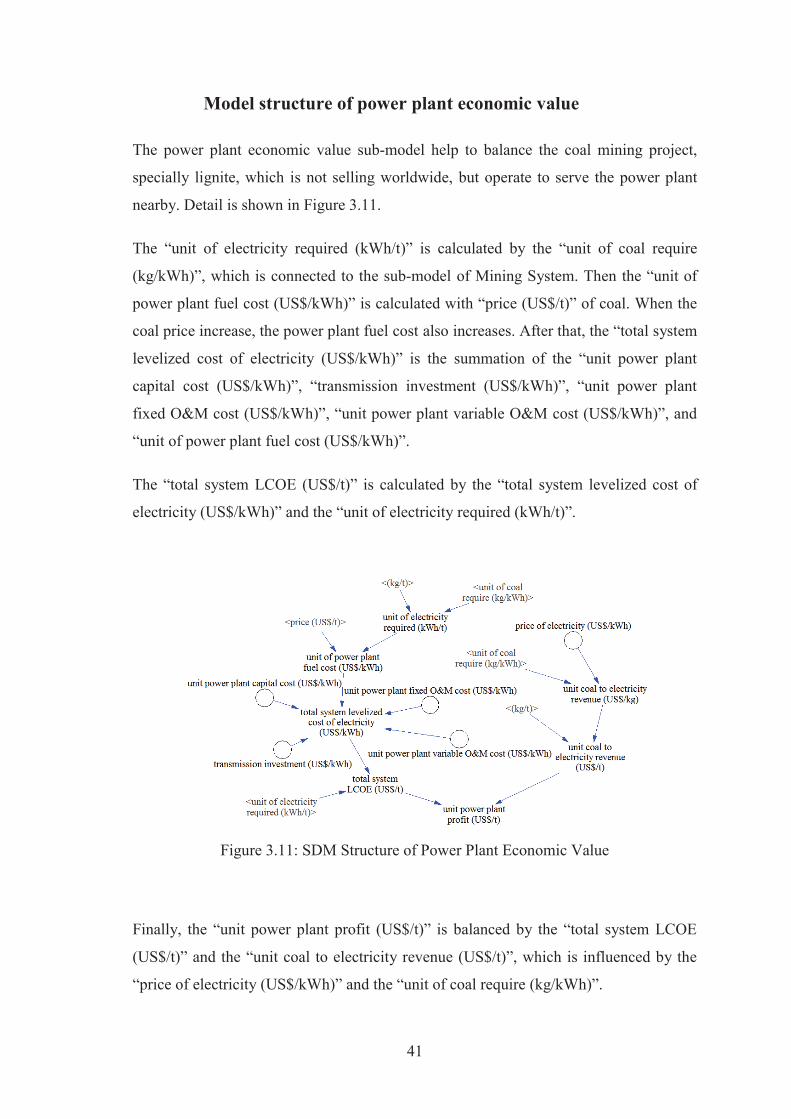
41
Model structure of power plant economic value
The power plant economic value sub-model help to balance the coal mining project,
specially lignite, which is not selling worldwide, but operate to serve the power plant
nearby. Detail is shown in Figure 3.11.
The “unit of electricity required (kWh/t)” is calculated by the “unit of coal require
(kg/kWh)”, which is connected to the sub-model of Mining System. Then the “unit of
power plant fuel cost (US$/kWh)” is calculated with “price (US$/t)” of coal. When the
coal price increase, the power plant fuel cost also increases. After that, the “total system
levelized cost of electricity (US$/kWh)” is the summation of the “unit power plant
capital cost (US$/kWh)”, “transmission investment (US$/kWh)”, “unit power plant
fixed O&M cost (US$/kWh)”, “unit power plant variable O&M cost (US$/kWh)”, and
“unit of power plant fuel cost (US$/kWh)”.
The “total system LCOE (US$/t)” is calculated by the “total system levelized cost of
electricity (US$/kWh)” and the “unit of electricity required (kWh/t)”.
Figure 3.11: SDM Structure of Power Plant Economic Value
Finally, the “unit power plant profit (US$/t)” is balanced by the “total system LCOE
(US$/t)” and the “unit coal to electricity revenue (US$/t)”, which is influenced by the
“price of electricity (US$/kWh)” and the “unit of coal require (kg/kWh)”.
42
3.3 Chapter Conclusion
The system dynamics model is a tool or methodology to understand the behaviour of a
system and solve problems, by using computer simulation software. In this thesis, the
system dynamics theory and methodology is used to analyse the complex system of coal
mining, which has many interconnected variables. The development of the model is
summarised in the following sections.
Firstly, the analytical information of general mining and coal mining is collected, and
then the variables and relationships, or equations between them are found. Secondly, the
knowledge is transferred into either a mental model or a causal loop diagram. After that,
the details are analysed of the relationships of the variables, which were connected in
the flow diagram or conceptual diagram. The research approach and SD model
development of the thesis is proposed, (Figure 3.1). Then, the analytical mapping of a
causal loop diagram (CLD) for a mining system, shown in Figure 3.2 (p. 29). Then, the
CLD is used to analyse the parameters and relationship of each parameter, to become
the economic conceptual diagram; see Figure 3.3 (p. 30) and Figure 3.4 (p. 31).
Then, the conceptual diagram is converted to a system dynamics structure, making it
more complex. The SDM structure can be developed manually by drawing on paper,
and later transferred to computer software, or be directly developed within the software.
In this research, Vensim Software is used to develop the SDM structure and to connect
all of the variables from general theory and literature reviews. Vensim Software has
many tools and functions to support the simulation behaviour of the variable, and also a
verifying tool to check model structure and mathematical analysis of the variable units.
Finally, all of the conceptual diagrams for project planning, in Figure 3.3 - Figure 3.5,
are analysed and the variable extended before converting to the SDM structure, see
details in Figure 3.6 - Figure 3.11. This is then put into the equations, and underwent
some other steps to become a prototype model.
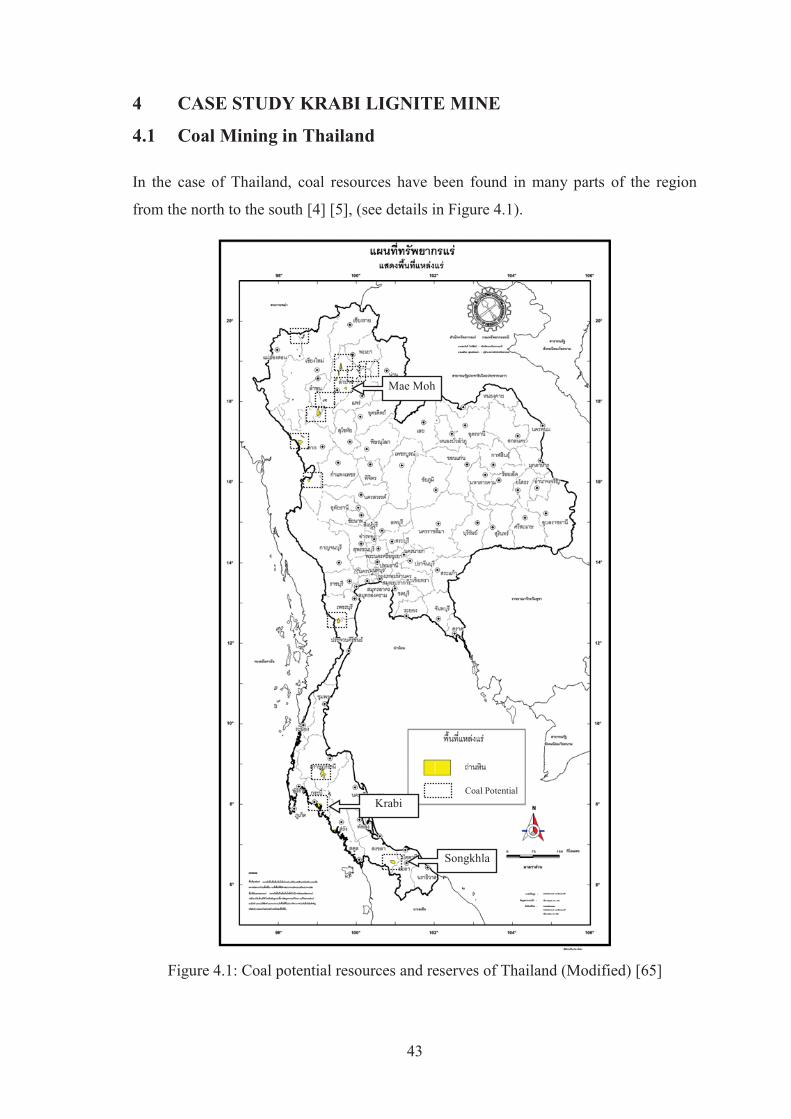
43
4 CASE STUDY KRABI LIGNITE MINE
4.1 Coal Mining in Thailand
In the case of Thailand, coal resources have been found in many parts of the region
from the north to the south [4] [5], (see details in Figure 4.1).
Figure 4.1: Coal potential resources and reserves of Thailand (Modified) [65]
Mae Moh
Krabi Coal Potential
Songkhla

44
Information on coal and electricity of Thailand
Thailand’s installed electricity capacity in 2011 was 31,447 MW, an increase of 527
MW from 30,920 MW in 2010. The Electricity Generating Authority of Thailand
(EGAT) provides the largest share at 48%. Next to this are Independent Power
Producers (IPP), providing a share of 38%; then Small Power Producers (SPP), 7%; and
power purchased from foreign sources, 7% [66].
The electricity peak load in 2011 occurred on the 24th May, reaching 24,518 MW; this
was 112 MW lower than the 2010 peak load of 24,630 MW, or a decrease of 0.5%. In
early 2011 the weather was still cold, coupled with early rainfall in the summer, this
made the temperature in the summer lower than that in the previous year [66], thus
people used less electricity.
Domestic lignite production of Thailand.
Domestic lignite production came previously from two major sources – one is the mines
belonging to the Electricity Generating Authority of Thailand (EGAT), and the other is
mines belonging to private producers. The EGAT’s sources comprised production from
the Mae Moh mine in the Lampang province (in northern Thailand), (Figure 4.1, p. 43),
and from the Krabi mine in the Krabi province (in southern Thailand). Lignite produced
from the Mae Moh mine is entirely used as fuel for power generation at the Mae Moh
Power Plant, while that from Krabi served the demand in the industrial sector. However,
production at the Krabi mine diminished substantially in output and was eventually
discontinued in 2008 [66, 67], detail is shown in Table II.1 (p. 166).
As for lignite production from the mines of private producers, the production volume
gradually dropped off because major domestic lignite concessions expired one after
another. Most of the lignite produced from the private sector mines is used in such
industries as cement, paper, food, and textile [66]. The trend of lignite production in
Thailand is shown in the Figure 4.2.
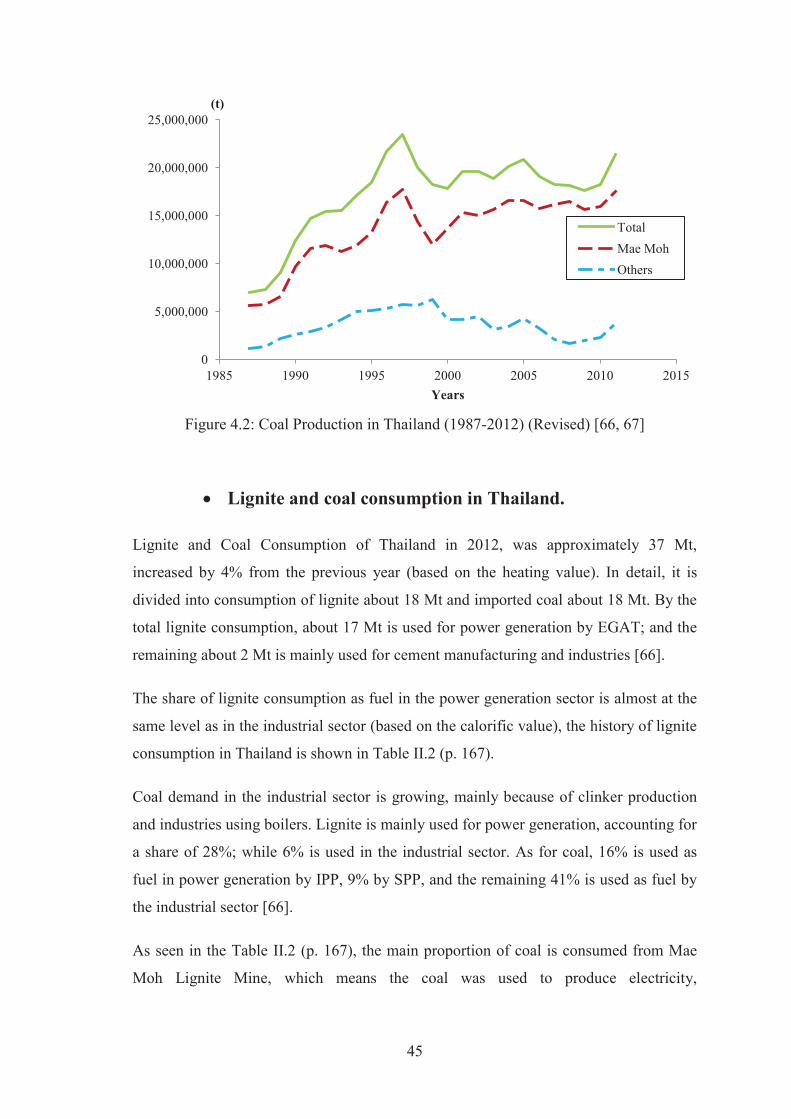
45
Figure 4.2: Coal Production in Thailand (1987-2012) (Revised) [66, 67]
Lignite and coal consumption in Thailand.
Lignite and Coal Consumption of Thailand in 2012, was approximately 37 Mt,
increased by 4% from the previous year (based on the heating value). In detail, it is
divided into consumption of lignite about 18 Mt and imported coal about 18 Mt. By the
total lignite consumption, about 17 Mt is used for power generation by EGAT; and the
remaining about 2 Mt is mainly used for cement manufacturing and industries [66].
The share of lignite consumption as fuel in the power generation sector is almost at the
same level as in the industrial sector (based on the calorific value), the history of lignite
consumption in Thailand is shown in Table II.2 (p. 167).
Coal demand in the industrial sector is growing, mainly because of clinker production
and industries using boilers. Lignite is mainly used for power generation, accounting for
a share of 28%; while 6% is used in the industrial sector. As for coal, 16% is used as
fuel in power generation by IPP, 9% by SPP, and the remaining 41% is used as fuel by
the industrial sector [66].
As seen in the Table II.2 (p. 167), the main proportion of coal is consumed from Mae
Moh Lignite Mine, which means the coal was used to produce electricity,
0
5,000,000
10,000,000
15,000,000
20,000,000
25,000,000
1985 1990 1995 2000 2005 2010 2015
(t)
Years
Total Mae Moh Others
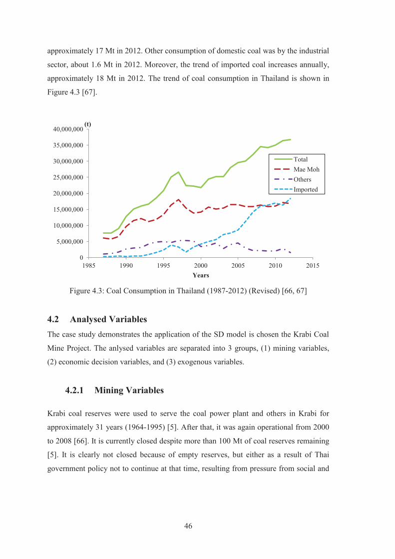
46
approximately 17 Mt in 2012. Other consumption of domestic coal was by the industrial
sector, about 1.6 Mt in 2012. Moreover, the trend of imported coal increases annually,
approximately 18 Mt in 2012. The trend of coal consumption in Thailand is shown in
Figure 4.3 [67].
Figure 4.3: Coal Consumption in Thailand (1987-2012) (Revised) [66, 67]
4.2 Analysed Variables The case study demonstrates the application of the SD model is chosen the Krabi Coal
Mine Project. The anlysed variables are separated into 3 groups, (1) mining variables,
(2) economic decision variables, and (3) exogenous variables.
4.2.1 Mining Variables
Krabi coal reserves were used to serve the coal power plant and others in Krabi for
approximately 31 years (1964-1995) [5]. After that, it was again operational from 2000
to 2008 [66]. It is currently closed despite more than 100 Mt of coal reserves remaining
[5]. It is clearly not closed because of empty reserves, but either as a result of Thai
government policy not to continue at that time, resulting from pressure from social and
0
5,000,000
10,000,000
15,000,000
20,000,000
25,000,000
30,000,000
35,000,000
40,000,000
1985 1990 1995 2000 2005 2010 2015
(t)
Years
Total Mae Moh Others Imported
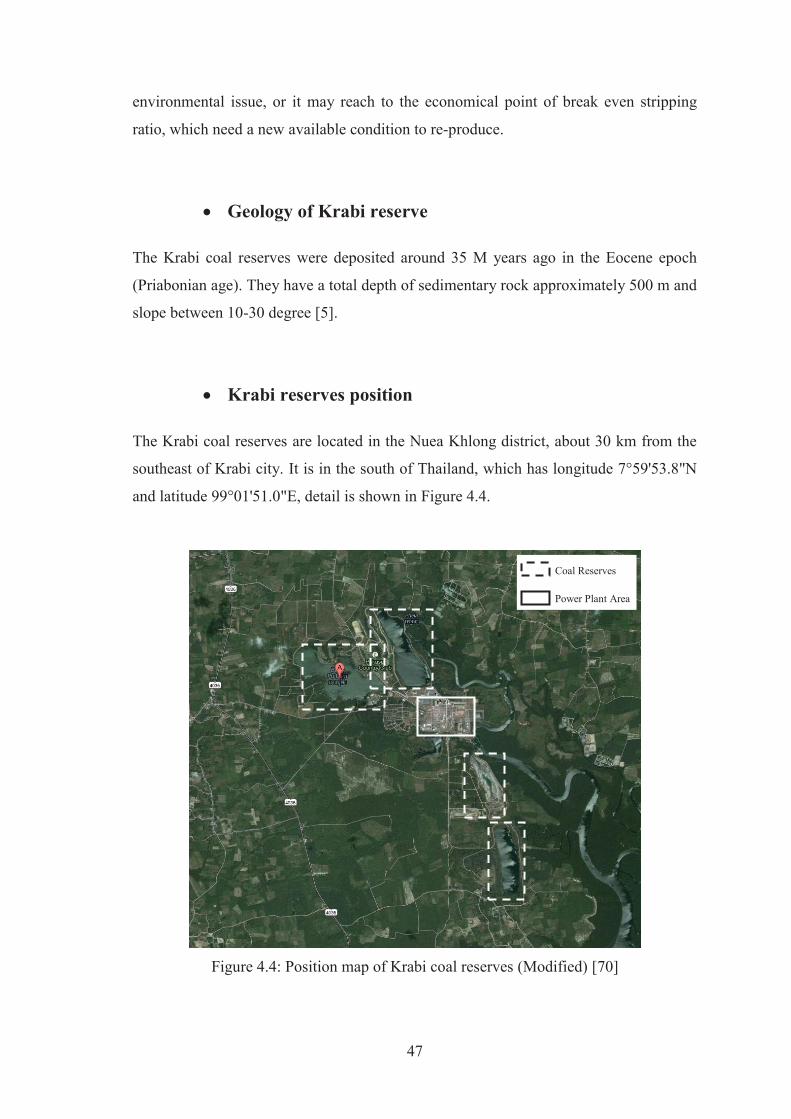
47
environmental issue, or it may reach to the economical point of break even stripping
ratio, which need a new available condition to re-produce.
Geology of Krabi reserve
The Krabi coal reserves were deposited around 35 M years ago in the Eocene epoch
(Priabonian age). They have a total depth of sedimentary rock approximately 500 m and
slope between 10-30 degree [5].
Krabi reserves position
The Krabi coal reserves are located in the Nuea Khlong district, about 30 km from the
southeast of Krabi city. It is in the south of Thailand, which has longitude 7°59'53.8"N
and latitude 99°01'51.0"E, detail is shown in Figure 4.4.
Figure 4.4: Position map of Krabi coal reserves (Modified) [70]
Power Plant Area
Coal Reserves
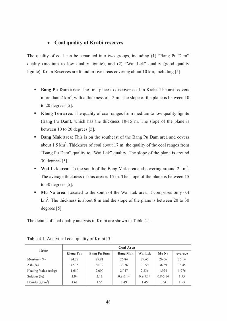
48
Coal quality of Krabi reserves
The quality of coal can be separated into two groups, including (1) “Bang Pu Dam”
quality (medium to low quality lignite), and (2) “Wai Lek” quality (good quality
lignite). Krabi Reserves are found in five areas covering about 10 km, including [5]:
Bang Pu Dam area: The first place to discover coal in Krabi. The area covers
more than 2 km2, with a thickness of 12 m. The slope of the plane is between 10
to 20 degrees [5].
Klong Ton area: The quality of coal ranges from medium to low quality lignite
(Bang Pu Dam), which has the thickness 10-15 m. The slope of the plane is
between 10 to 20 degrees [5].
Bang Mak area: This is on the southeast of the Bang Pu Dam area and covers
about 1.5 km2. Thickness of coal about 17 m; the quality of the coal ranges from
“Bang Pu Dam” quality to “Wai Lek” quality. The slope of the plane is around
30 degrees [5].
Wai Lek area: To the south of the Bang Mak area and covering around 2 km2.
The average thickness of this area is 15 m. The slope of the plane is between 15
to 30 degrees [5].
Mu Na area: Located to the south of the Wai Lek area, it comprises only 0.4
km2. The thickness is about 8 m and the slope of the plane is between 20 to 30
degrees [5].
The details of coal quality analysis in Krabi are shown in Table 4.1.
Table 4.1: Analytical coal quality of Krabi [5]
Items Coal Area
Klong Ton Bang Pu Dam Bang Mak Wai Lek Mu Na Average
Moisture (%) 24.22 25.91 26.84 27.65 26.66 26.14
Ash (%) 42.75 36.32 33.76 30.59 36.39 36.45
Heating Value (cal/g) 1,610 2,000 2,047 2,236 1,924 1,976
Sulphur (%) 1.94 2.11 0.8-5.14 0.8-5.14 0.8-5.14 1.95
Density (g/cm3) 1.61 1.55 1.49 1.45 1.54 1.53

49
Coal resources in Krabi
The calculation of coal resources in Krabi uses a cut off ash grade of 60% and heating
value of 1 kcal/g, details are shown in Table 4.2 [5].
Table 4.2: Analytical coal resources in Krabi [5]
Area Resources of Krabi (Mt)
Measured Indicated Total Klong Ton 13.50 8.97 32.47 Bang Pu Dam 27.06 27.06 Bang Mak 14.93 7.65 22.58 Wai Lek 24.62 18.21 42.83 Mu Na 3.50 3.50
Sum 83.61 44.83 128.45
Previous Krabi Lignite Mine activities
Krabi mining became operational in 1964, the steps of the operation can divide into 3
phases [5];
1st Phase: from June 1964, Krabi Lignite Mine had a stripping ratio 0.5-1.0:1
m3/t, used draglines with a bucket capacity of 1.912 m3, and trucks with a 12 t
loading capacity. Then, because the lignite seam was harder than the
overburden, the equipment was changed to a rope shovel with a bucket capacity
of 1.15 m3 [5]
2nd Phase: When the Krabi power plant had completed construction, the demand
of lignite increased to support the power plant, and the stripping ratio changed to
2.5-3.0:1 m3/t. The equipment was modified to a new rope shovel with a bucket
capacity of 2-2.5 m3, and the truck “EUCLID” with a 13.6 t loading capacity. In
this phase (since 1968), because of increased production planning requirements,
a subcontractor has helped in the achievement of production targets [5].
3rd Phase: The working site had 2 extensions, the “Wai Lek” site, which opened
in 1978 and had a stripping ratio of 6:1 m3/t; and the “Klong Bang Mak” site,
which opened in 1992 and had a stripping ratio of 2.68:1 m3/t. Although mining
50
ceased in 1995 [5], the mine was again operational between 2000 to 2008,
during that time it produced approximately 734,750 t [66].
Reclamation activity of Krabi Lignite Mine
The Krabi Lignite Mine is a surface mine, thus having a significant impact on the area.
EGAT prepared a master plan for the reclamation of the area, which assessed and
analysed the condition of the area prior to mining activity, so as to recover this
condition after mining. Therefore, the final design of the Krabi Lignite Mine stated that
after the closure the area be reclaimed by forests and reservoirs in the ratio of 72% and
28% respectively [5].
To support the sustainability of the reclamation and the closure activities in Krabi,
EGAT created a fund, depositing approximately 0.13 US$/t of Lignite produced [5].
Summary of previous Krabi Lignite Mine activity
There were originally estimated to be 128.45 Mt of lignite resources. Between 1964 to
1995, approximately 29.49 Mm3 of topsoil and overburden were moved, and 7.73 Mt of
lignite operated [5] Between 2000 to 2008, approximately 0.74 Mt of lignite were
produced [66]. Hence, in the Krabi Lignite reserves there remains about 120 Mt of
lignite.
Krabi coal power plant
The Krabi Lignite Power Plant is the only power plant in southern Thailand, which uses
lignite as a raw material. The total capacity of this power plant is 60 MW, coming from
three generating units. The Krabi Lignite Power Plant stopped operating in 1995
because of 31 years of use and also strong social and environmental concern [71]. At
that time, the south of Thailand had a sufficient electricity supply for the demand.
51
However, at the present status, the demand for electricity in southern Thailand is around
2,200-2,300 MW, while the electricity supply is only 1,600-1,800 MW [20]. Therefore,
the Thai Government, with EGAT, has proposed a project to create a new Krabi Coal
Power Plant on the previous site, and using clean coal technology. It is planned to being
operated in 2019 with a capacity of 800 MW [72].
4.2.2 Economic Decision Variables
The decision to investment in terms of economic criteria normally uses Net Present
Value (NPV). The main target of this simulation is to find the conditions, which
maximize the NPV of the mining project. It also supports more informed for decision
by Net Cash Flow of the project. The Net Cash Flow focuses the money in term of
amount of money flow into the project and flow out of the project. While, NPV focuses
the money in terms of value of money in a whole period of the project, and calculated
back to a present value. Therefore, two basis decision criteria, which are Net Cash Flow
and NPV, are chosen.
However, in this thesis when mining project has expansion cost as social and
environmental protection cost, and mine closure cost, which are separated and managed
by mining fund. The mining company cannot get any profit from mining fund, but it is
the responsibility of the mining company to pay enough money into a mining fund.
Therefore, the two new criteria are created, which are Net Cash Balance and NPV
Balance. The summary of the decision criteria variable definition is:
Net Cash Flow is the Summation of Cash Flow of The Mining Project,
Net Present Value is the Summation of DCF of The Mining Project,
Net Cash Balance is NCF with Summation of Cash Flow of Mining Fund,
NPV Balance is NPV with Summation of DCF of Mining Fund.
Finally, the NPV Balance is the new main decision criteria of the mining project,
because of covering time value of money and mining fund for a better social and
environmental protection and mine closure management.
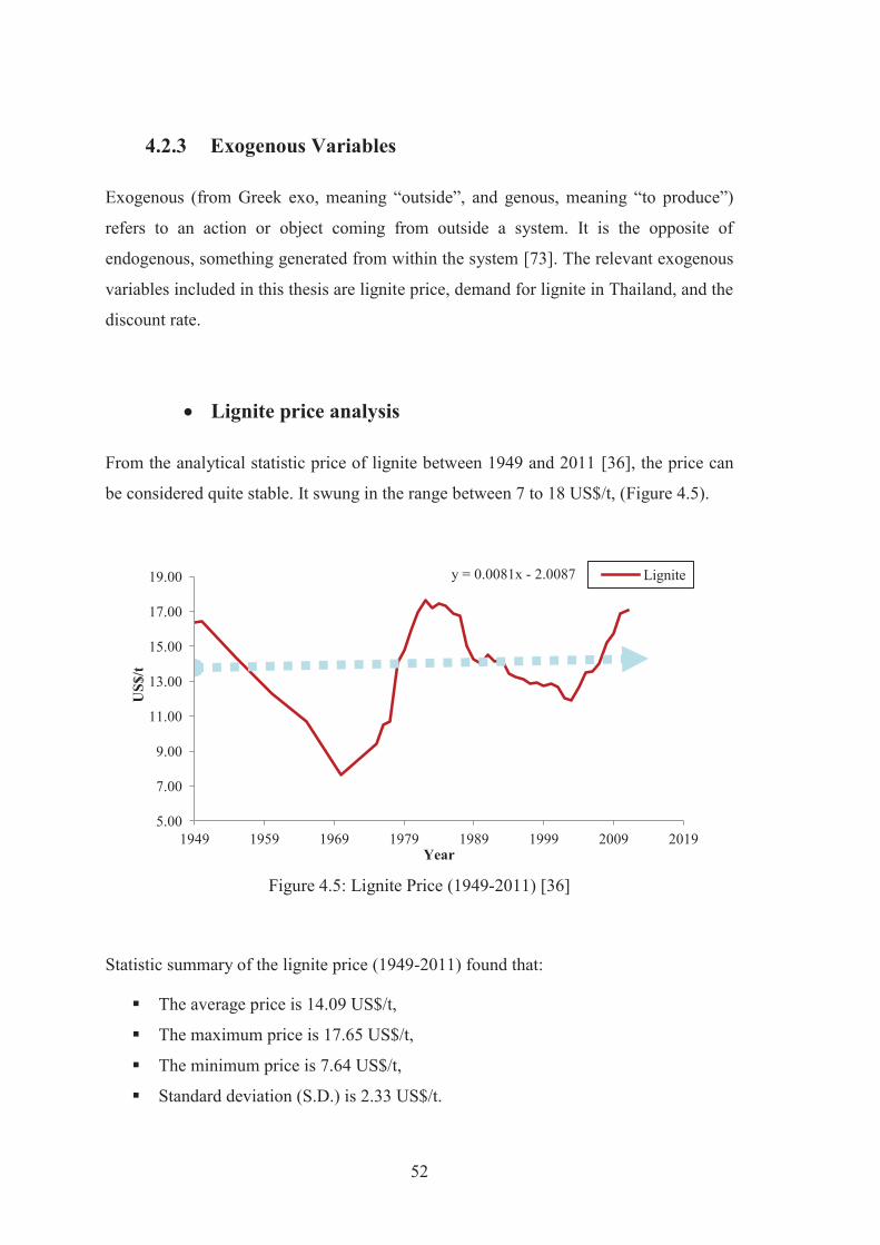
52
4.2.3 Exogenous Variables
Exogenous (from Greek exo, meaning “outside”, and genous, meaning “to produce”)
refers to an action or object coming from outside a system. It is the opposite of
endogenous, something generated from within the system [73]. The relevant exogenous
variables included in this thesis are lignite price, demand for lignite in Thailand, and the
discount rate.
Lignite price analysis
From the analytical statistic price of lignite between 1949 and 2011 [36], the price can
be considered quite stable. It swung in the range between 7 to 18 US$/t, (Figure 4.5).
Figure 4.5: Lignite Price (1949-2011) [36]
Statistic summary of the lignite price (1949-2011) found that:
The average price is 14.09 US$/t,
The maximum price is 17.65 US$/t,
The minimum price is 7.64 US$/t,
Standard deviation (S.D.) is 2.33 US$/t.
y = 0.0081x - 2.0087
5.00
7.00
9.00
11.00
13.00
15.00
17.00
19.00
1949 1959 1969 1979 1989 1999 2009 2019
US$
/t
Year
Lignite
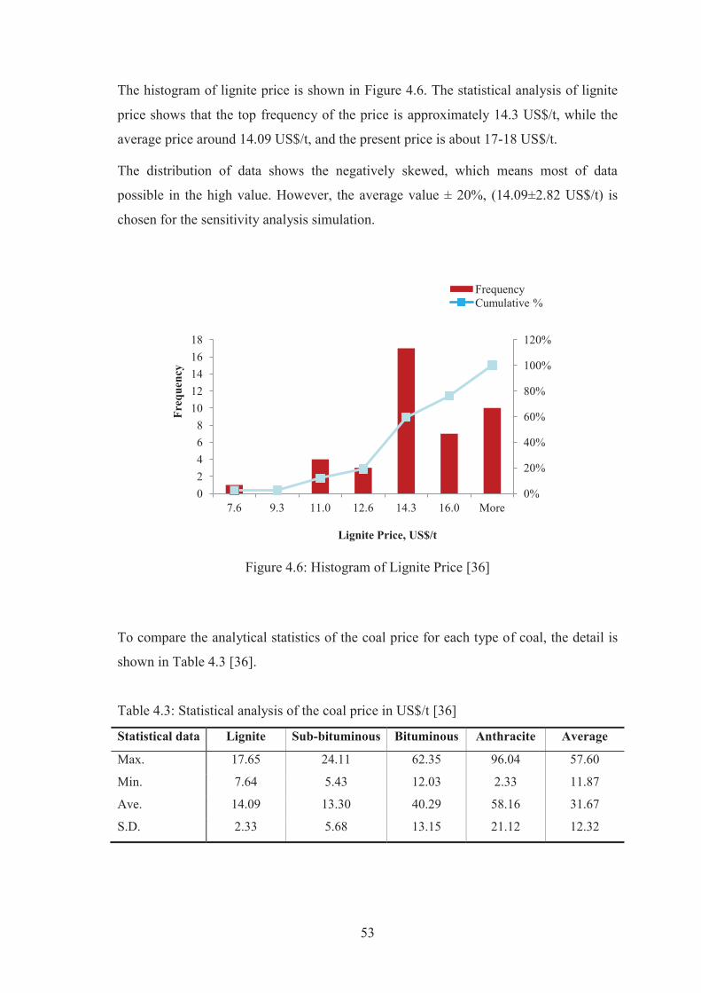
53
The histogram of lignite price is shown in Figure 4.6. The statistical analysis of lignite
price shows that the top frequency of the price is approximately 14.3 US$/t, while the
average price around 14.09 US$/t, and the present price is about 17-18 US$/t.
The distribution of data shows the negatively skewed, which means most of data
possible in the high value. However, the average value ± 20%, (14.09±2.82 US$/t) is
chosen for the sensitivity analysis simulation.
Figure 4.6: Histogram of Lignite Price [36]
To compare the analytical statistics of the coal price for each type of coal, the detail is
shown in Table 4.3 [36].
Table 4.3: Statistical analysis of the coal price in US$/t [36]
Statistical data Lignite Sub-bituminous Bituminous Anthracite Average
Max. 17.65 24.11 62.35 96.04 57.60
Min. 7.64 5.43 12.03 2.33 11.87
Ave. 14.09 13.30 40.29 58.16 31.67
S.D. 2.33 5.68 13.15 21.12 12.32
0%
20%
40%
60%
80%
100%
120%
0 2 4 6 8
10 12 14 16 18
7.6 9.3 11.0 12.6 14.3 16.0 More
Freq
uenc
y
Lignite Price, US$/t
Frequency Cumulative %

54
Demand of lignite in Thailand
In Thailand, the demand of lignite relies on two things: (1) demand of electricity, and
(2) policy of the Thai Government towards the use of lignite for producing electricity.
Nowadays, Mae Moh Lignite Mine produces approximately 17 Mt/y of lignite to
support the production of electricity; that creates approximately 18,000M units/y or
2,400 MW for a power plant (~12% of the electricity demand of Thailand, 2011) [4].
The electricity plan for Thailand is created by the Energy Policy and Planning Office, at
the Ministry of Energy. Due to increasing demand for electricity every year, so the
added capacity had to be planned. The added requirement during 2012 - 2030 of
approximately 55,130 MW could be fulfilled by power plant types as the Table 4.4 [74]:
Table 4.4: Energy plan of Thailand 2012-2030 [74]
Types Planning
Capacity Unit
1. Renewable energy power plants
- Power purchase from domestic
- Power purchase from neighbouring countries
14,580
9,481
5,099
MW
MW
MW
2. Cogeneration 6,476 MW
3. Combined cycle power plants 25,451 MW
4. Thermal power plants
- Coal-fired power plants
- Nuclear power plants
- Gas turbine power plants
- Power purchase from neighbouring countries
8,623
4,400
2,000
750
1,473
MW
MW
MW
MW
MW
Total 55,130 MW
Coal-fired power plants will be constructed to provide 4,400 MW between 2012 to
2030. The source of coal for the coal-fired power plant comes from two sources; firstly
from the domestic lignite of Thailand, and secondly, by importing from other countries.

55
The project planning phase of the Krabi Lignite Power Plant is currently in the process
of public hearings after completing a pre-study of environmental health impact
assessment (EHIA) [72].
The demand of coal can be estimated by energy consumption, which is related to the coal
heating value and the efficiency of the power plant technology. The sample calculation of
coal demand related to the coal condition of the Krabi reserves, shows below.
Coal demand calculation
Electrical energy is normally measured in “units” (1 unit is 1 kilowatt-hour or kWh).
However, energy is measured in the Joules (J), and a watt (W) is 1 joule per second
(J/s). So, 1 kWh is 1,000x60x60 joules = 3.6 MJ [75]. Now, to release 3.6 MJ from coal
at an average 40% efficiency of heat to electricity [76], and the average heating value of
the Krabi reserves as 1,976 kcal/kg [5], while 1 cal = 4.18 J, then 1,976x4.18 = 8,259.68
kJ/kg (~8.26 MJ/kg).
Thus, the production of 1 kWh of electricity by using lignite from the Krabi reserves
requires (3.6/(8.26x0.4)) = 1.09 kg of lignite. Moreover, in the case of Mae Moh Lignite
Mine, where there is an average heating value of lignite of 2,502 kcal/kg, approximately
0.86 kg/kWh is required.
Thailand discount rate analysis
Discount rate is a parameter, which represents the risk of investment decisions. The
discount rate has to be chosen to calculate NPV. On one hand, when selecting a low
value for the discount rate, this gradually reduces the value of money over time, which
may make Net Present Value (NPV) higher than zero. The decision to invest in a project
is “Accepted” when the NPV is higher than zero [9].
However, the project may fail and lose money when put into action, if the real risk is
higher than the chosen discount rate. On the other hand, when selecting a high value for
the discount rate, this significantly reduces the value of money over time, which will
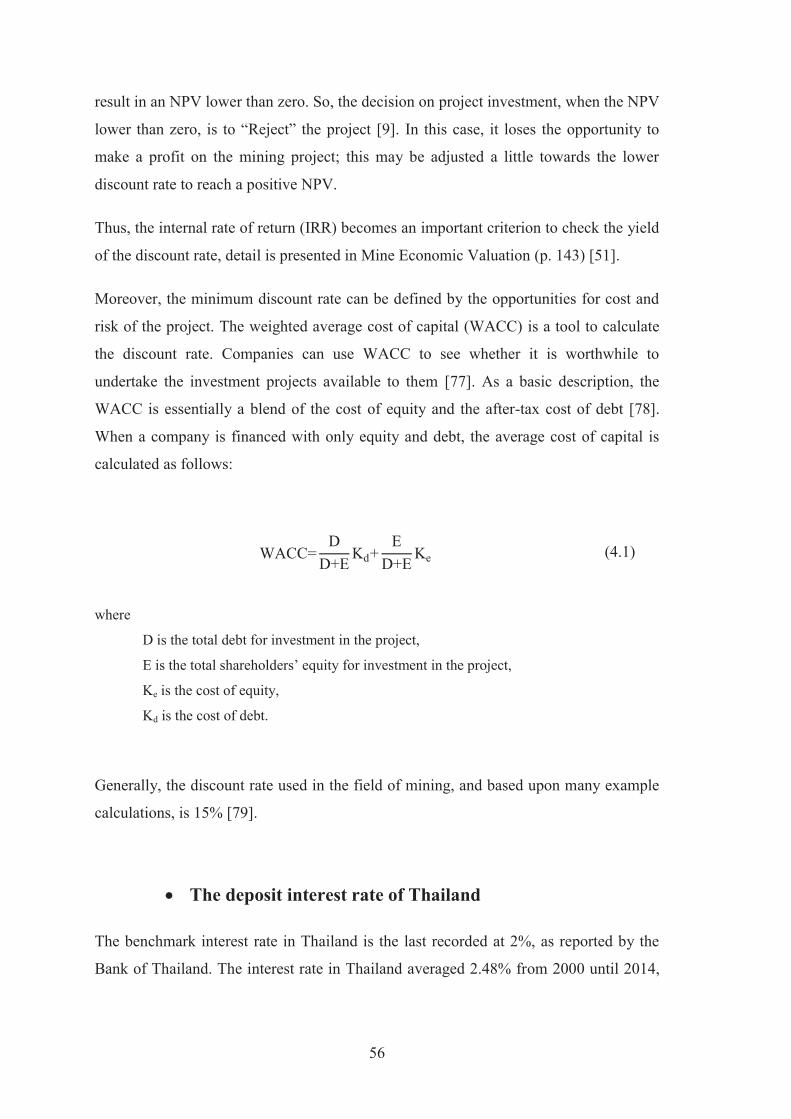
56
result in an NPV lower than zero. So, the decision on project investment, when the NPV
lower than zero, is to “Reject” the project [9]. In this case, it loses the opportunity to
make a profit on the mining project; this may be adjusted a little towards the lower
discount rate to reach a positive NPV.
Thus, the internal rate of return (IRR) becomes an important criterion to check the yield
of the discount rate, detail is presented in Mine Economic Valuation (p. 143) [51].
Moreover, the minimum discount rate can be defined by the opportunities for cost and
risk of the project. The weighted average cost of capital (WACC) is a tool to calculate
the discount rate. Companies can use WACC to see whether it is worthwhile to
undertake the investment projects available to them [77]. As a basic description, the
WACC is essentially a blend of the cost of equity and the after-tax cost of debt [78].
When a company is financed with only equity and debt, the average cost of capital is
calculated as follows:
WACC=D
D+EKd+
ED+E
Ke (4.1)
where
D is the total debt for investment in the project,
E is the total shareholders’ equity for investment in the project,
Ke is the cost of equity,
Kd is the cost of debt.
Generally, the discount rate used in the field of mining, and based upon many example
calculations, is 15% [79].
The deposit interest rate of Thailand
The benchmark interest rate in Thailand is the last recorded at 2%, as reported by the
Bank of Thailand. The interest rate in Thailand averaged 2.48% from 2000 until 2014,
57
reaching an all time high of 5% in June of 2006 and a record low of 1.25% in June of
2003. In Thailand, interest rate decisions are taken by The Bank of Thailand’s Monetary
Policy Committee [80]. Detail is shown in Figure 4.7.
Figure 4.7: Interest Rate Policy of Thailand (2005-2014) [81]
The inflation rate of Thailand
The inflation rate in Thailand was recorded at 1.96% in February of 2014, as presented
by the Bureau of Trade and Economic Indices, Ministry of Commerce, Thailand.
Inflation rate in Thailand averaged 4.59% from 1977 until 2014, reaching an all time the
highest of 24.56% in June 1980 and a record the lowest of -4.38% in July 2009.
In Thailand, the most important categories in the consumer price index are; food, which
is 33% of total index; transportation and communication, 27%; housing and furnishing,
23.5%; health care, 7%; recreation and education, 5%, electricity, fuel and water supply
5%; and apparel and footwear 3% [82]. Detail is shown in Figure 4.8.
y = -0.1544x + 313.13
-
1.00
2.00
3.00
4.00
5.00
6.00
2005 2007 2009 2011 2013 2015 2017
Inte
rest
rat
e (%
)
Years
Annual average rate …
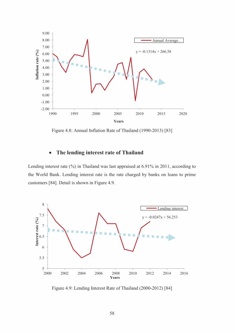
58
Figure 4.8: Annual Inflation Rate of Thailand (1990-2013) [83]
The lending interest rate of Thailand
Lending interest rate (%) in Thailand was last appraised at 6.91% in 2011, according to
the World Bank. Lending interest rate is the rate charged by banks on loans to prime
customers [84]. Detail is shown in Figure 4.9.
Figure 4.9: Lending Interest Rate of Thailand (2000-2012) [84]
y = -0.1314x + 266.58
-2.00
-1.00
0.00
1.00
2.00
3.00
4.00
5.00
6.00
7.00
8.00
9.00
1990 1995 2000 2005 2010 2015 2020
Infla
tion
rate
(%)
Years
Annual Average …
y = -0.0247x + 56.253
5
5.5
6
6.5
7
7.5
8
2000 2002 2004 2006 2008 2010 2012 2014 2016
Inte
rest
rat
e (%
)
Years
Lending interest …

59
Summary the suitable project discount rate of Thailand
The minimum project discount rate is estimated from the WACC, which depends upon
the economic condition of the nation. In this example, the metric calculation of the
deposit interest rate, the lending interest rate, and the inflation rate of Thailand was
analysed. The upper limit value is utilised in the simulation scenario and sensitivity
analysis of this thesis. The summary of the Thai discount rate analysis is shown in the
Table 4.5.
Table 4.5: Statistical analysis of the discount rate [80, 82, 84]
Statistical
Items
Lending Interest Rate (A)
Deposit Interest Rate (B)
Inflation Rate (C)
Discount Rate 1st
(B+C) 2nd
(A+B) 3rd
(A+C) Mean 6.65 2.82 3.61 6.43 9.47 10.26 S.D. 0.78 1.02 2.16 3.18 1.80 2.94 Min. 5.50 1.35 -0.80 0.55 6.85 4.70 Max. 7.80 4.79 8.10 12.89 12.59 15.90
Therefore, a 3rd discount rate, as 10.26%, is chosen for the simulation scenarios and
sensitivity analysis of this thesis. This is selected as it provides the maximum value,
which best covers the risk and opportunity cost of investment, at a minimum acceptable
value of the project.
4.3 Model Verification
During the development of the SD model and before using in the case study, the
verification of the SD model is important. There are four steps to verify and validate the
model, including, (1) logical checking, (2) model structure checking, (3) model unit
checking, and finally, (4) compared calculation result with real data.
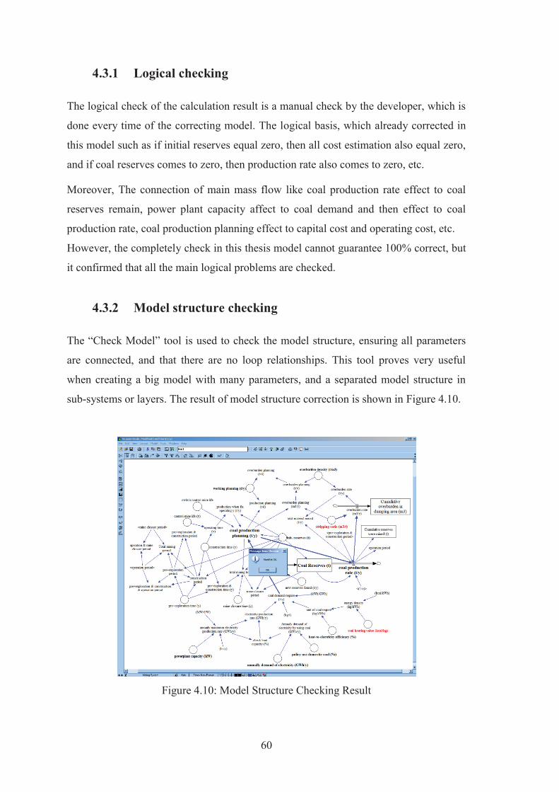
60
4.3.1 Logical checking
The logical check of the calculation result is a manual check by the developer, which is
done every time of the correcting model. The logical basis, which already corrected in
this model such as if initial reserves equal zero, then all cost estimation also equal zero,
and if coal reserves comes to zero, then production rate also comes to zero, etc.
Moreover, The connection of main mass flow like coal production rate effect to coal
reserves remain, power plant capacity affect to coal demand and then effect to coal
production rate, coal production planning effect to capital cost and operating cost, etc.
However, the completely check in this thesis model cannot guarantee 100% correct, but
it confirmed that all the main logical problems are checked.
4.3.2 Model structure checking
The “Check Model” tool is used to check the model structure, ensuring all parameters
are connected, and that there are no loop relationships. This tool proves very useful
when creating a big model with many parameters, and a separated model structure in
sub-systems or layers. The result of model structure correction is shown in Figure 4.10.
Figure 4.10: Model Structure Checking Result
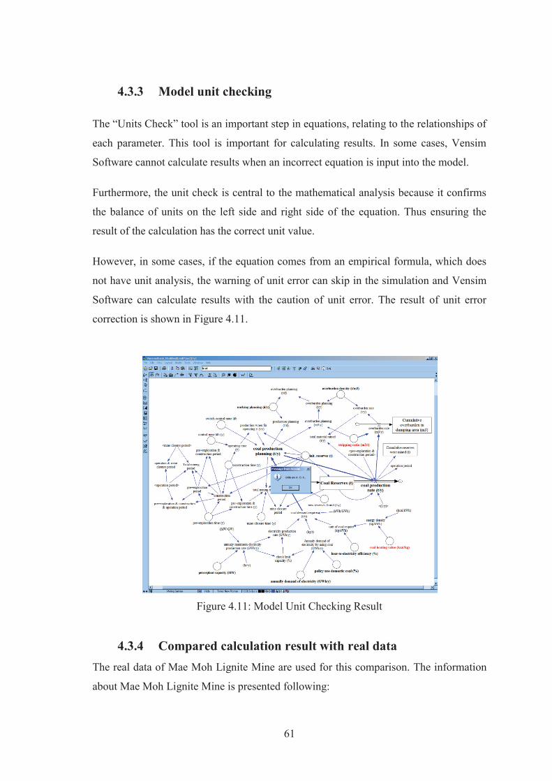
61
4.3.3 Model unit checking
The “Units Check” tool is an important step in equations, relating to the relationships of
each parameter. This tool is important for calculating results. In some cases, Vensim
Software cannot calculate results when an incorrect equation is input into the model.
Furthermore, the unit check is central to the mathematical analysis because it confirms
the balance of units on the left side and right side of the equation. Thus ensuring the
result of the calculation has the correct unit value.
However, in some cases, if the equation comes from an empirical formula, which does
not have unit analysis, the warning of unit error can skip in the simulation and Vensim
Software can calculate results with the caution of unit error. The result of unit error
correction is shown in Figure 4.11.
Figure 4.11: Model Unit Checking Result
4.3.4 Compared calculation result with real data The real data of Mae Moh Lignite Mine are used for this comparison. The information
about Mae Moh Lignite Mine is presented following:
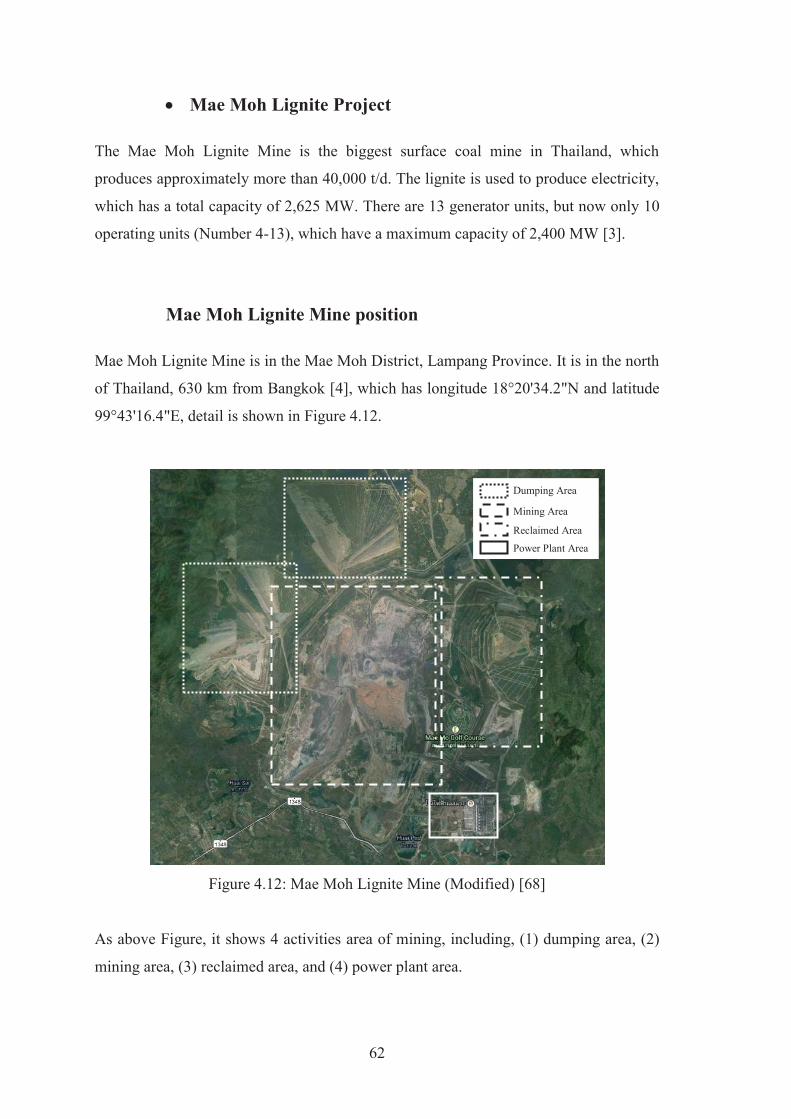
62
Mae Moh Lignite Project
The Mae Moh Lignite Mine is the biggest surface coal mine in Thailand, which
produces approximately more than 40,000 t/d. The lignite is used to produce electricity,
which has a total capacity of 2,625 MW. There are 13 generator units, but now only 10
operating units (Number 4-13), which have a maximum capacity of 2,400 MW [3].
Mae Moh Lignite Mine position
Mae Moh Lignite Mine is in the Mae Moh District, Lampang Province. It is in the north
of Thailand, 630 km from Bangkok [4], which has longitude 18°20'34.2"N and latitude
99°43'16.4"E, detail is shown in Figure 4.12.
Figure 4.12: Mae Moh Lignite Mine (Modified) [68]
As above Figure, it shows 4 activities area of mining, including, (1) dumping area, (2)
mining area, (3) reclaimed area, and (4) power plant area.
Dumping Area
Mining Area
Reclaimed Area
Power Plant Area
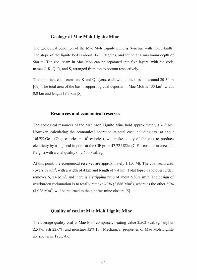
63
Geology of Mae Moh Lignite Mine
The geological condition of the Mae Moh Lignite mine is Syncline with many faults.
The slope of the lignite bed is about 10-30 degrees, and found at a maximum depth of
580 m. The coal seam in Mae Moh can be separated into five layers, with the code
names J, K, Q, R, and S, arranged from top to bottom respectively.
The important coal seams are K and Q layers, each with a thickness of around 20-30 m
[69]. The total area of the basin supporting coal deposits in Mae Moh is 135 km2, width
8.8 km and length 18.3 km [5].
Resources and economical reserves
The geological resources of the Mae Moh Lignite Mine hold approximately 1,468 Mt.
However, calculating the economical operation at total cost including tax, at about
10US$/Gcal (Giga calories = 109 calories), will make equity of the cost to produce
electricity by using coal imports at the CIF price 47.72 US$/t (CIF = cost, insurance and
freight) with a coal quality of 2,600 kcal/kg.
At this point, the economical reserves are approximately 1,150 Mt. The coal seam area
covers 38 km2, with a width of 4 km and length of 9.4 km. Total topsoil and overburden
removes 6,714 Mm3, and there is a stripping ratio of about 5.83:1 m3/t. The design of
overburden reclamation is to totally remove 40% (2,686 Mm3), where as the other 60%
(4,028 Mm3) will be returned to the pit after mine closure [5].
Quality of coal at Mae Moh Lignite Mine
The average quality coal at Mae Moh comprises, heating value 2,502 kcal/kg, sulphur
2.54%, ash 22.6%, and moisture 32% [5]. Mechanical properties of Mae Moh Lignite
are shown in Table 4.6.
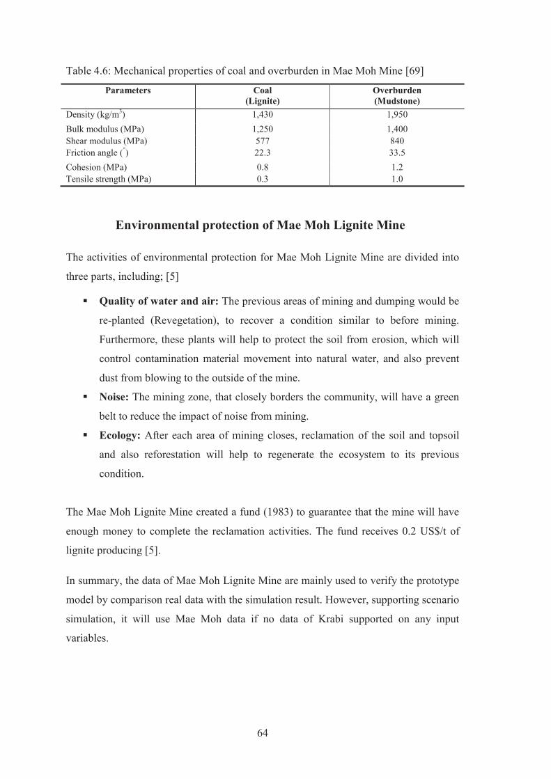
64
Table 4.6: Mechanical properties of coal and overburden in Mae Moh Mine [69]
Parameters Coal (Lignite)
Overburden (Mudstone)
Density (kg/m3) 1,430 1,950 Bulk modulus (MPa) 1,250 1,400 Shear modulus (MPa) 577 840 Friction angle (°) 22.3 33.5 Cohesion (MPa) 0.8 1.2 Tensile strength (MPa) 0.3 1.0
Environmental protection of Mae Moh Lignite Mine
The activities of environmental protection for Mae Moh Lignite Mine are divided into
three parts, including; [5]
Quality of water and air: The previous areas of mining and dumping would be
re-planted (Revegetation), to recover a condition similar to before mining.
Furthermore, these plants will help to protect the soil from erosion, which will
control contamination material movement into natural water, and also prevent
dust from blowing to the outside of the mine.
Noise: The mining zone, that closely borders the community, will have a green
belt to reduce the impact of noise from mining.
Ecology: After each area of mining closes, reclamation of the soil and topsoil
and also reforestation will help to regenerate the ecosystem to its previous
condition.
The Mae Moh Lignite Mine created a fund (1983) to guarantee that the mine will have
enough money to complete the reclamation activities. The fund receives 0.2 US$/t of
lignite producing [5].
In summary, the data of Mae Moh Lignite Mine are mainly used to verify the prototype
model by comparison real data with the simulation result. However, supporting scenario
simulation, it will use Mae Moh data if no data of Krabi supported on any input
variables.

65
Result of the comparison
The last step of model verification is checking the calculations of the model against real
data. In this research, the real data used to validate the results are historical data on the
production rate of Mae Moh Lignite Mine. The coal production rate results can be
calculated using input parameters including, electricity consumption, and policy of
using domestic coal in the model.
Then, from comparing the simulation result with the real data, it shows a significant of
the same trend of real data and simulation result. Detail of the comparison graph result
is shown in Figure 4.13.
Figure 4.13: Comparison of Mae Moh Production by Real Data and Simulation
When the comparison result shows a good significant of the model calculation
compared with the real data. Then, the model can go to the next step, which is
conditions setup for case study simulation.
4,000,000
6,000,000
8,000,000
10,000,000
12,000,000
14,000,000
16,000,000
18,000,000
20,000,000
1985 1990 1995 2000 2005 2010 2015 2020 2025
(t)
Years
Simulation (t) Mae Moh Production (t)

66
4.4 Simulation Conditions Setup
After the prototype model has been completely validated, the information about the case
study and all associated assumptions are put in as the input variables for sensitivity
analysis, scenario simulation, and optimum funding. The basic procedure of this
calculation step is shown in Figure 4.14.
Figure 4.14: Procedure of Simulation Result Making
The simulation is started by selecting input variables and assigning data to those
variables. The simulation is run to get results, which are then checked against the
criteria. If the criteria are not met, then the value or the variable must be changed. If the
results are logical, they can be used result values for decision making.

67
4.4.1 Sensitivity Analysis Conditions
The sensitivity analysis is used to analyse the input variables, which cannot be
controlled by a mining company, and their effect on the target variables. In this case, the
uncontrolled input variables are, price, stripping ratio, taxes, etc. The sensitivity of each
single variable will be analysed and performed the understanding of the combined effect
in the decision criteria variables, which are (1) Net Cash Flow, (2) Net Cash Balance,
(3) NPV, and (4) NPV Balance.
The Table 4.7 shows the list of input variables, which are used to perform the sensitivity
analysis of economic decision criteria on the Krabi Lignite Mine Project.
Table 4.7: List of input variable values used for sensitivity analysis
No. Input Parameters Average ±20% uncertainty 1 stripping ratio (m3/t) 3.38 2.23 - 4.53 2 coal heating value (kcal/kg) 1,976 1,320 – 2,632 3 deposit interest rate (%/y) 2.48 1.98 – 2.98 4 price (US$/t) 14.09 9.78 – 18.40 5 unit mine closure cost (US$/t) 0.52 0.42 – 0.62 6 unit S&EP cost (US$/t) 0.05 0.04 – 0.06 7 corporate tax rate (%) 25 16.47 – 33.53 8 discount rate (%) 10.26 8.21 – 12.31
The top four input variables of Table 4.7, which affect to the decision criterion
variables, are used to make the scenario simulation result.
4.4.2 Scenario Simulation Conditions
The case study simulation scenario focused on the new project Krabi Power Plant, with
a capacity of 800 MW, and operational in 2019 [72]. The preparation and construction
period takes around 5 years [20]. In this case study, it is assumed, that the Krabi Coal
Power Plant Project will use 100% domestic lignite; which approximately 120 Mt
lignite remain in Krabi [5].
The case study simulation is separated into four scenarios:

68
Constant Price Scenario: a scenario that uses the value at the present time or
the newest reference, which is found in the case study area or a general mining
information and theory. It is a base scenario, which always use in classical
assumption for a project evaluation and decision-making.
In Constant Price Scenario, it is assumed that the value of each variable remains
constant and steady for the entire period of the simulation, (Table 4.8).
Table 4.8: List of highlight input variable for Constant Price Scenario
No. Input Parameters Value 1 stripping ratio (m3/t) 6 2 coal heating value (kcal/kg) 1,976 3 deposit interest rate (%/y) 2.25 4 price (US$/t) 17.10 5 unit mine closure cost (US$/t) 0.52 6 unit S&EP cost (US$/t) 0.05 7 tax rate (%) 20 8 discount rate (%) 10.26 9 mining fund rate (US$/t) 0.13
Moreover, details of the full list of input variable values in Constant Price Scenario are
shown in Table II.3 (p. 168).
Normal Forecasting Price Scenario: a scenario that assumes the coal price
variable are going with the trend of the forecasting price data from the EIA,
which is increasing 1.4%/y [88], (F_Price_Norm).
Worst Forecasting Price Scenario: a scenario where the trend of price dropped
down 20% from a normal price forecasting data, (F_Price_Norm-20%).
Best Forecasting Price Scenario: a scenario, opposite to the worst case
scenario, in which the trend of price variable high up 20% from a normal price
forecasting data, (F_Price_Norm+20%).
In summary, the scenario simulation can make the situation of Krabi Lignite Mine
Project clearly. The constant price scenario is used for referencing the baseline situation
of this project. The forecasting price trend options are estimated from the coal price

69
forecasting by EIA (2014), which in the Normal Forecasting, the Worst Forecasting,
and the Best Forecasting, are clearly an alternative situation. Detail is shown in Figure
4.15.
Figure 4.15: Lignite Price Trend Forecasting (Modified) [88]
4.4.3 Optimum Funding Conditions
The optimum condition is where the target result reaches a maximum, minimum, or
specific value, with the changing of controllable input variables. The controllable
variables, such as production rate, working time, etc., are those variables, which the
mining company can adjust. The criteria of optimum condition are shown in Table 4.9.
Table 4.9: Criteria of the optimum condition
Objective: ; US$
Parameters Condition
Mining fund rate (MFR); US$/t 0 <= MFR <=Coal price; US$/t
In this research, the optimum condition of the “mining fund rate (US$/t)” is ascertained.
The mining company is to pay a small amount of money into the “mining fund” from
the “net revenue” generated to support the social and environmental protection and
mine closure period activities.
0.00
5.00
10.00
15.00
20.00
25.00
30.00
35.00
2000 2010 2020 2030 2040 2050
US$
/t
y
History Constant Normal Worst Best
History Forecasting
Present

70
5 CASE STUDY SIMULATION RESULTS AND DISCUSSION
5.1 Simulation Results of Krabi Lignite Mine Project
5.1.1 Sensitivity Analysis Results
The case study of Krabi Lignite Mine Project starts with the sensitivity analysis of the
input parameter for finding the significant input parameter for using in the scenario
simulation in the section 5.1.2, (p. 81). From the model structural development, the
eight input variables, which the mining company cannot control, are chosen to test the
sensitivity analysis including; (1) Price, (2) Stripping Ratio, (3) Coal Heating Value, (4)
Tax Rate, (5) Discount Rate, (6) Unit of Social and Environmental Cost, (7) Unit Mine
Closure Cost, and (8) Deposit Interest Rate.
The sensitivity analysis starts with an understanding of each input variable, which
already mention above, affect to the decision criteria variables of this thesis, which
including (1) Net Cash Flow, (2) Net Cash Balance, (3) NPV, and (4) NPV Balance.
The sensitivity analysis results of an input variable are following;
Coal price
Firstly, the coal price is chosen to check the sensitivity to the decision criteria, because
of the price in economic theory, its effects on demand and supply of the goods, and also
effects on the income of the project. In this case, it is focused on the direct effect of
price on the income of the mining project.
Actually, when the price increases, the revenue of the project also increases. Then, if the
costs are constant, the project will get more profit. Therefore, its effect on the Net Cash
Flow and NPV in the same direction.
From the historical data of lignite price, the average price is about 14.09 US$/t. To
understand how the lignite price effect on the decision criteria, it is assumed that there is
an uncertainty at ±20% of the average price. So it is varied from 11.27 to 16.91 US$/t.
The effects of price on each decision criteria are shown in Figure 5.1.
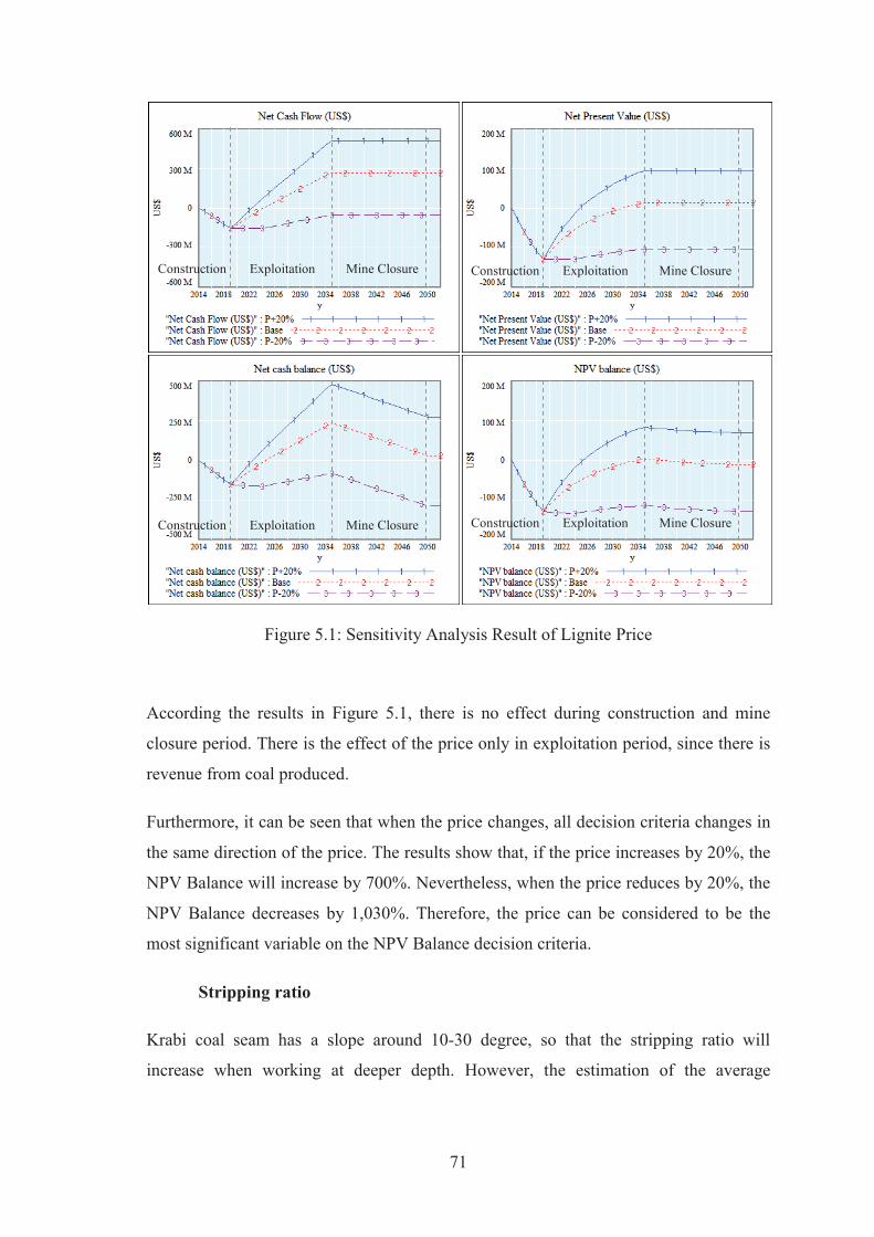
71
Figure 5.1: Sensitivity Analysis Result of Lignite Price
According the results in Figure 5.1, there is no effect during construction and mine
closure period. There is the effect of the price only in exploitation period, since there is
revenue from coal produced.
Furthermore, it can be seen that when the price changes, all decision criteria changes in
the same direction of the price. The results show that, if the price increases by 20%, the
NPV Balance will increase by 700%. Nevertheless, when the price reduces by 20%, the
NPV Balance decreases by 1,030%. Therefore, the price can be considered to be the
most significant variable on the NPV Balance decision criteria.
Stripping ratio
Krabi coal seam has a slope around 10-30 degree, so that the stripping ratio will
increase when working at deeper depth. However, the estimation of the average
Exploitation Mine Closure Construction
Exploitation Mine Closure Construction
Exploitation Mine Closure Construction
Exploitation Mine Closure Construction
72
stripping ratio is around 3.38 m3/t. Thus, if it is assumed the uncertainty at ±20% of
average value and at the same ratio of price variations, the stripping ratio will be varied
between 2.70 – 4.06 m3/t. The effects of stripping ratio on the decision criteria are
shown in Figure 5.2.
Figure 5.2: Sensitivity Analysis Result of Stripping Ratio
It can be seen from Figure 5.2 that there is an effect of stripping ratio variation at all the
three periods. Larger stripping ratio results on more overburden removed. It is obvious
that when the stripping ratio changes, all decision criteria change in the opposite
direction of the stripping ratio. When the stripping ratio increases, the amount of
overburden per unit of coal produced increases and so does the overburden removal
expenditure. It also affects mine closure cost and social and environmental protection
cost. Which affects the optimum mining fund rate.
Exploitation Mine Closure Construction
Exploitation Mine Closure Construction
Exploitation Mine Closure Construction
Exploitation Mine Closure Construction

73
In summary, if the stripping ratio increases 20%, the NPV Balance will decrease 397%.
On another hand, when the stripping ratio decreases by 20%, the NPV Balance will
increase by 371%. Therefore, stripping ratio can be considered to be the 2nd significant
variation in the NPV Balance decision criteria.
Coal heating value
The average heating value of Krabi lignite reserves is about 1,976 kcal/kg. If it has an
uncertainty of ±20% of average value, it would vary between 1,581 – 2,371 kcal/kg.
The effects of coal heating value to the decision criteria show in Figure 5.3.
Figure 5.3: Sensitivity Analysis Result of Coal Heating Value
There is an effect of coal heating value variation at all 3 periods. Coal heating value
affects on the amount of coal required for coal-fired power plant. It is found that when
the coal heating value changes, all decision criteria change in the opposite direction of
Exploitation Mine Closure Construction
Exploitation Mine Closure Construction
Exploitation Mine Closure Construction
Exploitation Mine Closure Construction
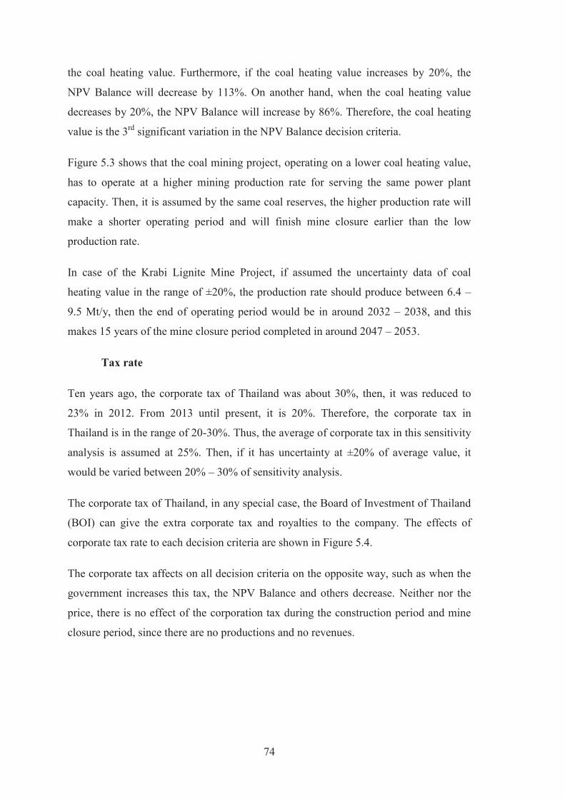
74
the coal heating value. Furthermore, if the coal heating value increases by 20%, the
NPV Balance will decrease by 113%. On another hand, when the coal heating value
decreases by 20%, the NPV Balance will increase by 86%. Therefore, the coal heating
value is the 3rd significant variation in the NPV Balance decision criteria.
Figure 5.3 shows that the coal mining project, operating on a lower coal heating value,
has to operate at a higher mining production rate for serving the same power plant
capacity. Then, it is assumed by the same coal reserves, the higher production rate will
make a shorter operating period and will finish mine closure earlier than the low
production rate.
In case of the Krabi Lignite Mine Project, if assumed the uncertainty data of coal
heating value in the range of ±20%, the production rate should produce between 6.4 –
9.5 Mt/y, then the end of operating period would be in around 2032 – 2038, and this
makes 15 years of the mine closure period completed in around 2047 – 2053.
Tax rate
Ten years ago, the corporate tax of Thailand was about 30%, then, it was reduced to
23% in 2012. From 2013 until present, it is 20%. Therefore, the corporate tax in
Thailand is in the range of 20-30%. Thus, the average of corporate tax in this sensitivity
analysis is assumed at 25%. Then, if it has uncertainty at ±20% of average value, it
would be varied between 20% – 30% of sensitivity analysis.
The corporate tax of Thailand, in any special case, the Board of Investment of Thailand
(BOI) can give the extra corporate tax and royalties to the company. The effects of
corporate tax rate to each decision criteria are shown in Figure 5.4.
The corporate tax affects on all decision criteria on the opposite way, such as when the
government increases this tax, the NPV Balance and others decrease. Neither nor the
price, there is no effect of the corporation tax during the construction period and mine
closure period, since there are no productions and no revenues.
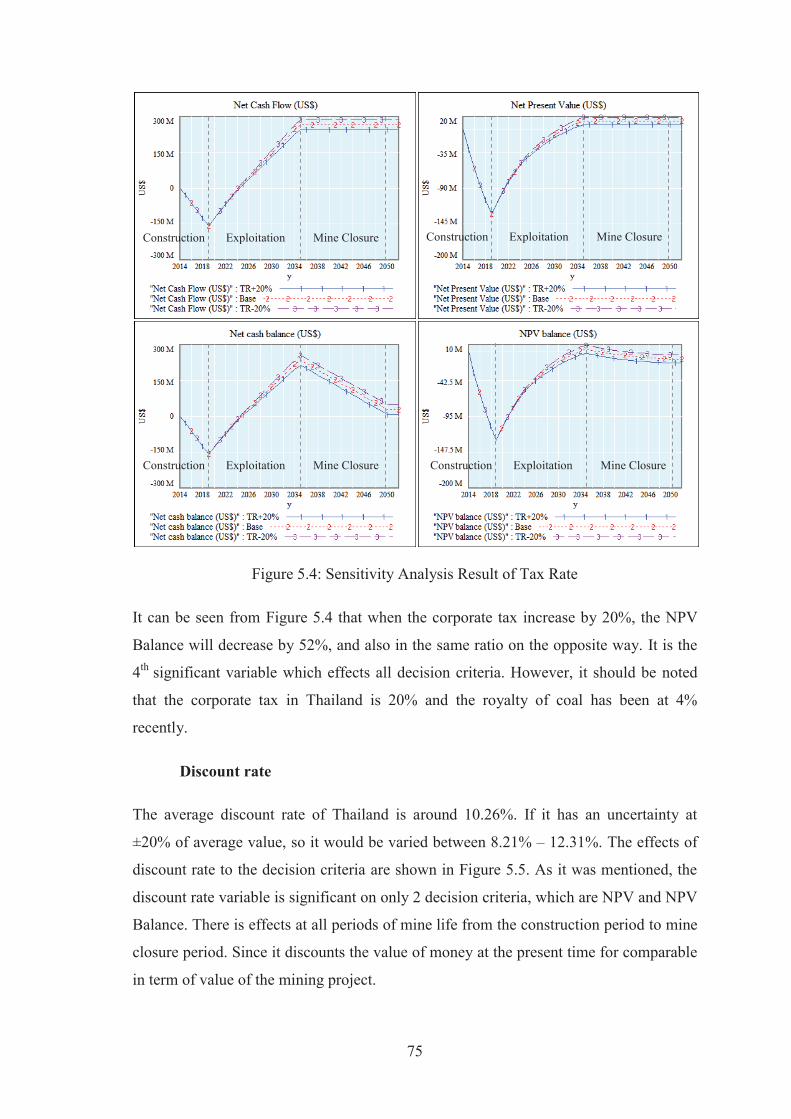
75
Figure 5.4: Sensitivity Analysis Result of Tax Rate
It can be seen from Figure 5.4 that when the corporate tax increase by 20%, the NPV
Balance will decrease by 52%, and also in the same ratio on the opposite way. It is the
4th significant variable which effects all decision criteria. However, it should be noted
that the corporate tax in Thailand is 20% and the royalty of coal has been at 4%
recently.
Discount rate
The average discount rate of Thailand is around 10.26%. If it has an uncertainty at
±20% of average value, so it would be varied between 8.21% – 12.31%. The effects of
discount rate to the decision criteria are shown in Figure 5.5. As it was mentioned, the
discount rate variable is significant on only 2 decision criteria, which are NPV and NPV
Balance. There is effects at all periods of mine life from the construction period to mine
closure period. Since it discounts the value of money at the present time for comparable
in term of value of the mining project.
Exploitation Mine Closure Construction
Exploitation Mine Closure Construction
Exploitation Mine Closure Construction
Exploitation Mine Closure Construction

76
Figure 5.5: Sensitivity Analysis Result of Discount Rate
The discount rate affects on NPV and NPV Balance in the opposite way, when the
discount rate increases by 20%, the NPV Balance will decrease by 109%. On another
hand, if the discount rate decreases by 20%, the NPV Balance will increase by 125%.
The discount rate could be the 3rd significant variable, if it is focused only two economic
decision criteria, NPV and NPV Balance.
Unit S&EP cost
Social and environmental protection cost can vary widely depending on the condition
such as, the degree of environmental effect, the activities to support social and
environmental protection, and etc. Assuming the average unit S&EP cost of Thailand is
about 0.05 US$/t. If it has an uncertainty at ±20% of average value, so it would be
varied between 0.04 – 0.06 US$/t. The effects of unit S&EP cost to the decision criteria
are shown in Figure 5.6.
Exploitation Mine Closure Construction
Exploitation Mine Closure Construction
Exploitation Mine Closure Construction
Exploitation Mine Closure Construction
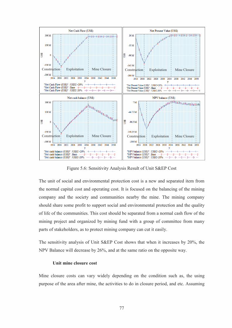
77
Figure 5.6: Sensitivity Analysis Result of Unit S&EP Cost
The unit of social and environmental protection cost is a new and separated item from
the normal capital cost and operating cost. It is focused on the balancing of the mining
company and the society and communities nearby the mine. The mining company
should share some profit to support social and environmental protection and the quality
of life of the communities. This cost should be separated from a normal cash flow of the
mining project and organized by mining fund with a group of committee from many
parts of stakeholders, as to protect mining company can cut it easily.
The sensitivity analysis of Unit S&EP Cost shows that when it increases by 20%, the
NPV Balance will decrease by 26%, and at the same ratio on the opposite way.
Unit mine closure cost
Mine closure costs can vary widely depending on the condition such as, the using
purpose of the area after mine, the activities to do in closure period, and etc. Assuming
Exploitation Mine Closure Construction
Exploitation Mine Closure Construction
Exploitation Mine Closure Construction
Exploitation Mine Closure Construction
78
the average unit mine closure cost in Thailand is about 0.52 US$/t. If it has uncertainty
at ±20% of average value, so it would be varied between 0.42 – 0.62 US$/t. The effects
of unit mine closure cost to the decision criteria are shown in Figure 5.7.
Figure 5.7: Sensitivity Analysis Result of Unit Mine Closure Cost
Nowadays, mine closure is an important activity after the end of mine operation,
because it is a final process before returning the land after mined to other activities in
the future. Activities in mine closure period need money for motivation. Nevertheless,
in mine closure period, mining company does not have income, so that some mining
company does not want to expend in this period. The mining fund is proposed to
guarantee the activities in mine closure period will be completely done.
Unit mine closure cost is one of the parameters related to the mining fund expenditure
activities. It would be multiplied by the ratio of overburden backfill to rehabilitate.
However, there is an effect of the unit mine closure cost only in the mine closure period.
Exploitation Mine Closure Construction
Exploitation Mine Closure Construction
Exploitation Mine Closure Construction
Exploitation Mine Closure Construction

79
When it increases by 20%, the NPV Balance will decrease by 25%, and on the opposite
way with the same ratio.
Deposit interest rate
The deposit interest rate of Thailand is about 2.48%. If it has an uncertainty at ±20% of
average value, so it would be varied between 1.98% to 2.98%. The effects of the deposit
interest rate to the decision criteria are shown in Figure 5.8.
Figure 5.8: Sensitivity Analysis Result of Deposit Interest Rate
The deposit interest rate affects on the mining fund directly. Whenever the mining fund
balance is in the positive part, the deposit interest rate will give an interest to the mining
fund balance. Otherwise, the deposit interest rate will not give any extra amount. In this
case, the mining fund rate of 0.13 US$/t is not enough for mining fund balance stays in
positive part, thus the deposit interest rate does not affect the mining fund. That is the
Exploitation Mine Closure Construction
Exploitation Mine Closure Construction
Exploitation Mine Closure Construction
Exploitation Mine Closure Construction
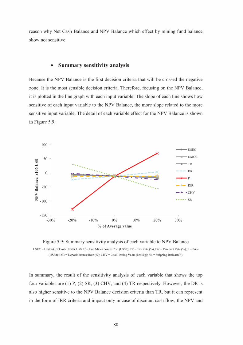
80
reason why Net Cash Balance and NPV Balance which effect by mining fund balance
show not sensitive.
Summary sensitivity analysis
Because the NPV Balance is the first decision criteria that will be crossed the negative
zone. It is the most sensible decision criteria. Therefore, focusing on the NPV Balance,
it is plotted in the line graph with each input variable. The slope of each line shows how
sensitive of each input variable to the NPV Balance, the more slope related to the more
sensitive input variable. The detail of each variable effect for the NPV Balance is shown
in Figure 5.9.
Figure 5.9: Summary sensitivity analysis of each variable to NPV Balance USEC = Unit S&EP Cost (US$/t); UMCC = Unit Mine Closure Cost (US$/t); TR = Tax Rate (%); DR = Discount Rate (%); P = Price
(US$/t); DIR = Deposit Interest Rate (%); CHV = Coal Heating Value (kcal/kg); SR = Stripping Ratio (m3/t).
In summary, the result of the sensitivity analysis of each variable that shows the top
four variables are (1) P, (2) SR, (3) CHV, and (4) TR respectively. However, the DR is
also higher sensitive to the NPV Balance decision criteria than TR, but it can represent
in the form of IRR criteria and impact only in case of discount cash flow, the NPV and
-150
-100
-50
0
50
100
-30% -20% -10% 0% 10% 20% 30%
NPV
Bal
ance
, x10
6 U
S$
% of Average value
USEC
UMCC
TR
DR
P
DIR
CHV
SR

81
the NPV Balance. Thus, the DR is arranged at 5th of sensitivity result, and IRR will be
found in each simulation scenario. The result of the analytical effects of the top four
variables is shown in the section 5.1.2.
5.1.2 Scenario Simulation Results
By using the top four sensitive variables of the mining project decision, the simulation
result can be separated into four scenarios; (1) the Constant Price Scenario, (2) the
Normal Forecasting Price Scenario, (3) the Worst Forecasting Price Scenario, and (4)
the Best Forecasting Price Scenario. Details of each scenario condition are shown in the
Table 4.8 in Chapter 3 (p. 68).
The constant price scenario
The Constant Price Scenario for the Krabi Lignite Mine Project starts with the
assumption that the price is constant at 17.1 US$/t, the stripping ratio at 6.0 m3/t, coal
heating value at 1,976 kcal/kg, tax at 20%, etc. Details of base simulation show in the
graph line number three (Figure 5.10).
As mention before, the NPV Balance is the first decision criteria, which will move to
the negative zone when input variable condition change. Base condition result,
(F_Price_Fix) in Figure 5.10 shows that the most criteria is in the negative zone. The
Net Cash Balance is -231.13 M US$, NPV is -39.51 M US$, and NPV Balance is -
85.30 M US$. An exception is for Net Cash Flow, which is still in the positive zone,
194.51 M US$. In this case, IRR of the NPV Balance cannot be estimated because the
Net Cash Balance is in the negative zone when balancing with the mining fund.
The tool is very helpful to find the critical condition. It is found that the critical price is
20 US$/t (F_Price_Fix CP), which makes the project feasible. In this condition, the Net
Cash Flow will be 458.33 M US$, the Net Cash Balance 32.69 M US$, and the Net
Present Value returns 46 M US$. The NPV Balance returns a positive value of 0.19 M
US$ (the graph line number two in Figure 5.10). In this case, mining operation will be
finished in 2035 and mine closure will be completed in 2050.
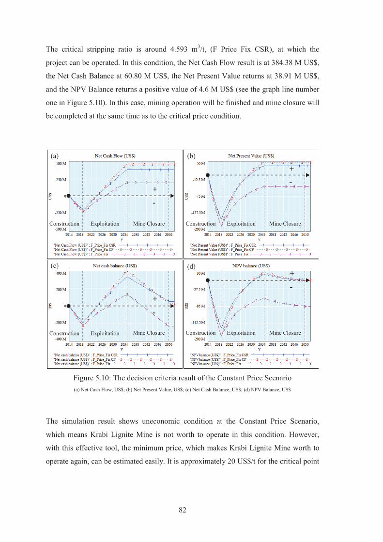
82
The critical stripping ratio is around 4.593 m3/t, (F_Price_Fix CSR), at which the
project can be operated. In this condition, the Net Cash Flow result is at 384.38 M US$,
the Net Cash Balance at 60.80 M US$, the Net Present Value returns at 38.91 M US$,
and the NPV Balance returns a positive value of 4.6 M US$ (see the graph line number
one in Figure 5.10). In this case, mining operation will be finished and mine closure will
be completed at the same time as to the critical price condition.
Figure 5.10: The decision criteria result of the Constant Price Scenario (a) Net Cash Flow, US$; (b) Net Present Value, US$; (c) Net Cash Balance, US$; (d) NPV Balance, US$
The simulation result shows uneconomic condition at the Constant Price Scenario,
which means Krabi Lignite Mine is not worth to operate in this condition. However,
with this effective tool, the minimum price, which makes Krabi Lignite Mine worth to
operate again, can be estimated easily. It is approximately 20 US$/t for the critical point
+
-
+
-
+
-
+
-
(a) (b)
(c) (d)
Exploitation Mine Closure Construction Exploitation Mine Closure Construction
Exploitation Mine Closure Construction Exploitation Mine Closure Construction

83
of lignite price, which will make Krabi Lignite Mine Project back to be profitable at the
end of mine life.
On the other hand, at the price 17.1 US$/t, the break even stripping ratio would be 4.593
m3/t. Therefore, in this condition, it is not recommended to operate Krabi Lignite Mine
Project for serving Krabi Coal Power Plant Project at this moment. Because the data of
Krabi lignite operation (2008) indicates the stripping ratio at 6.0 m3/t. Otherwise,
selective mining should be employed at the only zone which break even stripping ratio
is not higher than 4.593 m3/t.
Alternatively, underground coal mining method may be brought into consideration.In
this case, it is found that no critical point of corporation tax and the heating value,
which makes the situation of the project on profit. Therefore, the project should be
delayed until the lignite price goes more than 20 US$/t. This may be the most possible
way to make Krabi Lignite Mine Project on profit.
Therefore, the Krabi Lignite Mine Project would not be started based upon this
condition. Because of the negative value of the main decision criteria. Moreover, when
looking at the details of the mining fund, the mining fund rate of 0.13 US$/t for
reclamation is not suitable to cover the additional cost of social and environmental
protection and the mine closure cost. When looking at the Net Cash Balance, it also
confirms that the mining project does not have enough cash flow to pay for the extra
cost of social and environmental protection cost and mine closure cost.
The normal forecasting price scenario
Coal price was forecasted by EIA (2014) between 2012 – 2040 to rise 1.4% annually
[88]. At the same ratio, lignite price will be increased from 17.1 US$/t in 2014 to 29
US$/t in 2052. Other significant input variables include, the stripping ratio at 6.0 m3/t,
coal heating value at 1,976 kcal/kg, tax at 20%, etc. Details of base simulation are
shown in the graph line number four (Figure 5.11).
The base condition result, (F_Price_Norm), shows that most decision criteria is in the
positive zone. Net Cash Flow is 486.87 M US$, Net Cash Balance is 61.23 M US$, and
84
NPV is 38.87 M US$, but the NPV Balance is still in negative zone, -6.93 M US$. In
this case, IRR could be 9.63% for making NPV Balance at zero.
It is found that the critical coal heating value is 1,662.4 kcal/kg, (F_Price_Norm
CCHV), which makes the project possible to be operated in maximum profit with the
normal trend of price, constant stripping ratio and corporate tax. The coal heating value
is a complicated effect to the decision criteria variable, due to the fact that it does not
affect the NPV Balance and others directly. The effect comes from the effect on the
mining production rate. Then the mining production rate refers to mining size, which
affects on the capital cost and operating cost estimation. In the cost theory, the bigger
the mining production is, the cheaper unit cost per tonnes. On another hand, higher
production rate makes a higher amount of overburden and also environmental effects.
Therefore, the increasing in coal heating value can possibly increase or decrease NPV
Balance and other decision criteria depending on a specific situation.
The optimum coal heating value shows the Net Cash Flow result at 497.95 M US$, the
Net Cash Balance at 96.65 M US$, the Net Present Value returns at 59.96 M US$, and
the NPV Balance returns a positive value of 7.59 M US$ (see details in the graph line
number three in Figure 5.11). In this case, the mining operation will be finished in 2033
and mine closure will be completed in 2047.
The critical stripping ratio is about 5.86 m3/t, (F_Price_Norm CSR), which indicates
that the project can be operated. This condition shows the Net Cash Flow result at
504.93 M US$, the Net Cash Balance at 89.44 M US$, the Net Present Value returns at
45.53 M US$, and the NPV Balance returns a positive value of 0.88 M US$ (see the
graph line number two in Figure 5.11). In this case, the mining operation will be
finished in 2035 and mine closure will be completed in 2050.
In case of Thai Government needs to support Krabi Lignite Mine Project by special
corporate tax, the critical corporate tax should be around 16%, (F_Price_Norm CTR),
for which the Thai Government should not charge tax more than that value and the
project can be operated. This condition shows the Net Cash Flow result at 513.83 M
US$, the Net Cash Balance at 88.19 M US$, the Net Present Value returns at 45.80 M
US$, and the NPV Balance returns a positive value of 0.04 M US$ (see details in the

85
graph line number one in Figure 5.11). In this case, the mining operation will also be
finished in 2035 and mine closure will be completed in 2050.
Figure 5.11: The decision criteria result of the Normal Forecasting Price Scenario
(a) Net Cash Flow, US$; (b) Net Present Value, US$; (c) Net Cash Balance, US$; (d) NPV Balance, US$
The Normal Forecasting Price Scenario shows the alternative results of the critical value
in each significant input variable, when the price follows the EIA (2014) forecasting.
The idea of reducing an average coal heating value to 1,662.4 kcal/kg for feeding the
power plant, which makes a bigger mining production rate and reduces the cost per
tonne, should be checked with the minimum acceptable coal heating value of the power
plant. The break even stripping ratio found is at 5.86 m3/t. However, by the information
of Krabi Lignite Mine, the stripping ratio was done at 6.0 m3/t. Thus, the possible way
to do in this case is to make the selective mining only in the zone that the stripping ratio
is not greater than 5.86 m3/t, so that it can be operated economically. On another way,
+
-
+
-
+
- +
-
(a) (b)
(c) (d)
Exploitation Mine Closure Construction Exploitation Mine Closure Construction
Exploitation Mine Closure Construction Exploitation Mine Closure Construction
86
the idea of underground mining may be considered for the possibilities of technique,
technology, and mining cost.
The last critical point, which is not in the hands of any mining company, is the
corporate tax. It should not be more than 16%, which Thai Government can charge from
this project, while it is at 20% corporate tax recently.
Besides, this scenario is quite a good case example, which shows the difference
decision result between using NPV criteria and NPV Balance criteria. If the final
decision criterion is NPV, this project is feasible to operate, which mining company
does not have to pay any mining fund, or pay any amount of money without balancing
at the end of mine life (see graph (b) in Figure 5.11).
However, the most important economic criterion, which balancing the Mining Fund
with the Net Present Value of the Krabi Lignite Mine Project, is shown to result in an
NPV Balance variable with a negative amount, -6.93 M US$. Hence, the funding rate
that the Krabi Lignite Mine Project, which would have paid the expenditure of the
mining fund in this scenario, is not enough. At the end of the mine closure period, the
cumulative present value for the balancing of the mining fund is still bigger than the Net
Present Value of the Krabi Lignite Mine Project earnings, so it makes the summary
result in a negative amount. The NPV Balance is the most important criteria as it
includes time value of money and balancing of the mining fund.
Therefore, the Krabi Lignite Mine Project in the Normal Forecasting Price Scenario
condition is not feasible, which means rejecting this project scenario at this moment.
The worst forecasting price scenario
The Worst Forecasting Price Scenario of the Krabi Lignite Mine Project, which means a
20 % reduction of normal trend of price forecasting, is proposed. The Worst Forecasting
Price for the Krabi Lignite Mine Project helps to understand the possible worst situation
for the project on the forecasting price trend. This situation can happen if the demand of
coal reduces by using others alternative energy supply such as; natural gas, oil, or
renewable energy. Thus, in this case, coal price forecasting is 1.12%/y increasing,

87
which makes lignite price be increased in the lower rate of normal price trend
forecasting, from 17.1 US$/t in 2014 to 26.11 US$/t in 2052. By assuming other
significant input variables are constant (stripping ratio at 6.0 m3/t, coal heating value at
1,976 kcal/kg, tax at 20%, etc.). Details of base simulation are shown in the graph line
number three (Figure 5.12). The decision criteria base condition result, (F_Price_Norm-
20%), shows half of the decision criteria in positive zone, the Net Cash Flow is 422.51
M US$, NPV is 21.41 M US$, and in negative zone, Net Cash Balance is -3.13 M US$,
and the NPV Balance is -24.38 M US$.
In this case, the Net Cash Balance is lower than zero, which means that cash flow of the
project is not enough to support social and environmental protection and mine closure
cost. There is no IRR value, which makes NPV Balance equals zero. Therefore, in this
condition, the mining company should redesign land use after mine closure, reduce the
backfill ratio planning in order to make the Net Cash Balance of the project finish in the
positive zone.
The critical point of stripping ratio is about 5.69 m3/t, (F_Price_Norm-20% CSR),
which indicates that the project can be operated. This condition shows the Net Cash
Flow result at 469.87 M US$, the Net Cash Balance at 66.71 M US$, the Net Present
Value returns at 43.65 M US$, and the NPV Balance returns a positive value of 0.38 M
US$ (see the graph line number two in Figure 5.12). In this case, the mining operation
will be finished in 2035 and mine closure will be completed in 2050.
In case of Thai Government wants to support Krabi Lignite Mine Project by offering the
special corporate tax, it is about 4.22%, (F_Price_Norm-20% CTR) by which the
project can be operated. This condition shows the Net Cash Flow result at 518.06 M
US$, the Net Cash Balance at 92.42 M US$, the Net Present Value returns at 45.81 M
US$, and the NPV Balance returns a positive value of 0.02 M US$ (see the graph line
number one in Figure 5.12). In this case, the mining operation will also be finished
operating in 2035 and mine closure will be completed in 2050.
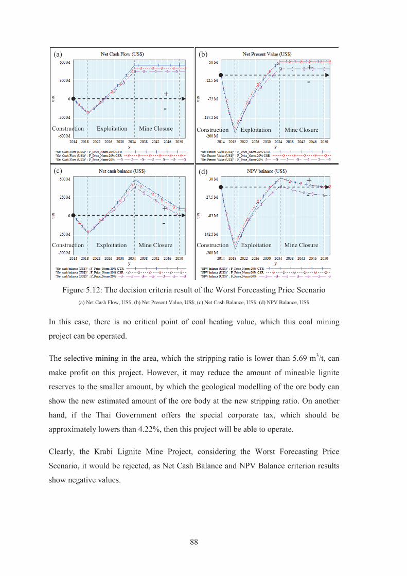
88
Figure 5.12: The decision criteria result of the Worst Forecasting Price Scenario
(a) Net Cash Flow, US$; (b) Net Present Value, US$; (c) Net Cash Balance, US$; (d) NPV Balance, US$
In this case, there is no critical point of coal heating value, which this coal mining
project can be operated.
The selective mining in the area, which the stripping ratio is lower than 5.69 m3/t, can
make profit on this project. However, it may reduce the amount of mineable lignite
reserves to the smaller amount, by which the geological modelling of the ore body can
show the new estimated amount of the ore body at the new stripping ratio. On another
hand, if the Thai Government offers the special corporate tax, which should be
approximately lowers than 4.22%, then this project will be able to operate.
Clearly, the Krabi Lignite Mine Project, considering the Worst Forecasting Price
Scenario, it would be rejected, as Net Cash Balance and NPV Balance criterion results
show negative values.
+
-
+
-
+
-
+
-
(a) (b)
(c) (d)
Exploitation Mine Closure Construction
Exploitation Mine Closure Construction Exploitation Mine Closure Construction
Exploitation Mine Closure Construction
89
The best forecasting price scenario
The Best Forecasting Price Scenario for the Krabi Lignite Mine Project used with the
assumption that demand of coal is increasing more than the normal price forecasting,
which can be happen in the following cases: the price of natural gas and oil increase
from a decline in supply, natural disaster, and etc. Furthermore, the clean coal
technology, policy, and the acceptance of the society to use coal can also make demands
of coal increasing, and then it will make the coal price increase in a higher rate than the
normal forecasting ratio. Assumed at 20% increases more than the normal trend
forecasting. Thus, in this case coal price forecasting is 1.68%/y, which makes the lignite
price rise from 17.1 US$/t in 2014 to 32.21 US$/t in 2052. Other significant input
variables constant include; the stripping ratio at 6.0 m3/t, coal heating value at 1,976
kcal/kg, tax at 20%, and etc. Details of base simulation show in the graph line number
four (Figure 5.13). The decision criteria base condition result, (F_Price_Norm+20%),
shows all of the decision criteria in positive zone, the Net Cash Flow is 553.64 M US$,
the NPV is 56.88 M US$, the Net Cash Balance is 128 M US$, and the NPV Balance is
11.08 M US$. In this condition, the IRR is found at 11.15%.
The optimum coal heating value, which can make the maximum value of NPV Balance,
is 1,683.24 kcal/kg, (F_Price_Norm+20% CCHV). In this condition, the Net Cash Flow
is 556.20 M US$, the NPV is 76.41 M US$, the Net Cash Balance is 154.90 M US$,
and the NPV Balance is 24.18 M US$. It is a special input parameter, because the coal
heating value makes mining production rate change, which affects on the operating
period and mine closure period. In this case, the mining operation will finish in 2033,
and mine closure in 2047. Detail is shown in the graph line number three, (Figure 5.13).
The critical stripping ratio is about 6.2 m3/t, (F_Price_Norm+20% CSR), which
indicates that the project can be operated. This condition shows the Net Cash Flow
result at 528.93 M US$, the Net Cash Balance as 88.78 M US$, the Net Present Value
returns at 47.73 M US$, and the NPV Balance returns a positive value of 0.30 M US$
(see the graph line number two in Figure 5.13). In this case, the mining operation will
be finished in 2035 and mine closure will be completed in 2050.
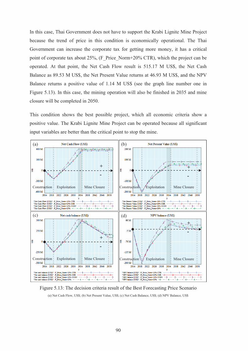
90
In this case, Thai Government does not have to support the Krabi Lignite Mine Project
because the trend of price in this condition is economically operational. The Thai
Government can increase the corporate tax for getting more money, it has a critical
point of corporate tax about 25%, (F_Price_Norm+20% CTR), which the project can be
operated. At that point, the Net Cash Flow result is 515.17 M US$, the Net Cash
Balance as 89.53 M US$, the Net Present Value returns at 46.93 M US$, and the NPV
Balance returns a positive value of 1.14 M US$ (see the graph line number one in
Figure 5.13). In this case, the mining operation will also be finished in 2035 and mine
closure will be completed in 2050.
This condition shows the best possible project, which all economic criteria show a
positive value. The Krabi Lignite Mine Project can be operated because all significant
input variables are better than the critical point to stop the mine.
Figure 5.13: The decision criteria result of the Best Forecasting Price Scenario
(a) Net Cash Flow, US$; (b) Net Present Value, US$; (c) Net Cash Balance, US$; (d) NPV Balance, US$
+
-
+
-
+
- +
-
(a) (b)
(c) (d)
Exploitation Mine Closure Construction Exploitation Mine Closure Construction
Exploitation Mine Closure Construction Exploitation Mine Closure Construction
91
Moreover, by using the tool, it is also found that the critical price trend in the case of
Krabi Lignite Mine Project condition is 1.51%/y. It means this project can start to
operate when the trend forecasting of coal price increasing at least 1.51%/y. Otherwise,
it should hold the project to operate until the suitable time.
Summary, the Krabi Lignite Mine Project in the Best Forecasting Price Scenario would
be completely accepted, because of the positive values on all economic criteria.
5.1.3 Optimum Funding Result
From the sensitivity analysis results and simulation scenarios by NPV Balance criteria,
almost scenarios simulations of the Krabi Lignite Mine Project are in the negative zone.
This means that if the Krabi Lignite Power Plant does wish to use the domestic lignite
in Krabi, it would not be feasible at this time. Only the Best Forecasting Price Scenario
shows the positive result, which can accept the project. However, the Normal
Forecasting Price Scenario is the most possibly condition by EIA (2014) forecasting the
price. Therefore, the Normal Forecasting Price Scenario is the best example, which is
chosen for finding optimum mining fund rate and IRR.
In the Normal Forecasting Price Scenario, the mining fund rate of 0.13 US$/t will be
deposited in the mining fund account. It is found that this mining fund not having
enough money for social and environmental protection and mine closure. However, it
may be possible to find the optimum result, which holds NPV positive and the mining
fund equal to zero at the end of mine life (detail is shown in Figure 5.14).
In case of the Normal Forecasting Price Scenario condition, the Mining Fund line
number three in Figure 5.14 moves to the negative zone, reaching a total debt of
approximately -425.6 M US$. While, the net cash flow of the mining company could be
486.87 M US$, so the Net Cash balance will still be at the positive, 61.23 M US$. It
means that if mining company has to pay for these costs directly, it is also possible to
pay, because the Net Cash Flow of the project still positive after balancing these cost.

92
Figure 5.14: Cumulative mining fund a long period of mine life
(a) Mining Fund Rate, US$/y; (b) Funding Balance, US$/y; (c) Income Fund Rate, US$/y; (d) Using Fund Rate, US$/y
Figure 5.15: Mining fund cash flow comparison
(a) (b)
(c) (d)
+
-
Exploitation Mine Closure Construction
Exploitation Mine Closure Construction Exploitation Mine Closure Construction
Exploitation Mine Closure Construction Exploitation Mine Closure Construction

93
However, if the mining company creates mining fund, and deposit money in that fund.
The mining fund can grow itself by deposit interest rate, which help the mining
company not need to pay in a total cost of social and environmental protection and mine
closure cost.
Therefore, this tool helped to find the minimum mining fund rate, 2.71 US$/t. It made
the cumulative mining fund growth reach the positive part, and ensure enough money to
cover until the end of the mine closure period. The detail of mining fund cash flow is
shown in Figure 5.15. Graph (a), the mining fund rate, which mining company pays
some amount of money only in the exploitation period annually. Graph (b), the annual
balancing of income of mining fund and expenditure of mining fund. Graph (c), the
annual income of mining fund, which grow by the deposit interest rate. Graph (d) the
annual cost of social and environmental protection and mine closure cost a long period
of exploitation and mine closure period.
(a) Net Cash Flow, US$; (b) Net Present Value, US$; (c) Net Cash Balance, US$; (d) NPV Balance, US$
Figure 5.16: The optimum mining fund on the Normal Forecasting Price Scenario
+
-
+
-
+
-
+
-
(a) (b)
(c) (d)
Exploitation Mine Closure Construction
Exploitation Mine Closure Construction Exploitation Mine Closure Construction
Exploitation Mine Closure Construction
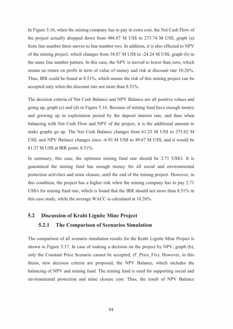
94
In Figure 5.16, when the mining company has to pay in extra cost, the Net Cash Flow of
the project actually dropped down from 486.87 M US$ to 273.74 M US$, graph (a)
from line number three moves to line number two. In addition, it is also effected to NPV
of the mining project, which changes from 38.87 M US$ to -24.24 M US$, graph (b) in
the same line number pattern. In this case, the NPV is moved to lower than zero, which
means no return on profit in term of value of money and risk at discount rate 10.26%.
Thus, IRR could be found at 8.51%, which means the risk of this mining project can be
accepted only when the discount rate not more than 8.51%.
The decision criteria of Net Cash Balance and NPV Balance are all positive values and
going up, graph (c) and (d) in Figure 5.16. Because of mining fund have enough money
and growing up in exploitation period by the deposit interest rate, and then when
balancing with Net Cash Flow and NPV of the project, it is the additional amount to
make graphs go up. The Net Cash Balance changes from 61.23 M US$ to 275.62 M
US$, and NPV Balance changes since -6.93 M US$ to 49.67 M US$, and it would be
81.37 M US$ at IRR point, 8.51%.
In summary, this case, the optimum mining fund rate should be 2.71 US$/t. It is
guaranteed the mining fund has enough money for all social and environmental
protection activities and mine closure, until the end of the mining project. However, in
this condition, the project has a higher risk when the mining company has to pay 2.71
US$/t for mining fund rate, which is found that the IRR should not more than 8.51% in
this case study, while the average WACC is calculated at 10.26%.
5.2 Discussion of Krabi Lignite Mine Project
5.2.1 The Comparison of Scenarios Simulation
The comparison of all scenario simulation results for the Krabi Lignite Mine Project is
shown in Figure 5.17. In case of making a decision on the project by NPV, graph (b),
only the Constant Price Scenario cannot be accepted, (F_Price_Fix). However, in this
thesis, new decision criteria are proposed, the NPV Balance, which includes the
balancing of NPV and mining fund. The mining fund is used for supporting social and
environmental protection and mine closure cost. Thus, the result of NPV Balance
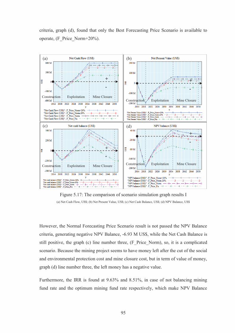
95
criteria, graph (d), found that only the Best Forecasting Price Scenario is available to
operate, (F_Price_Norm+20%).
Figure 5.17: The comparison of scenario simulation graph results I
(a) Net Cash Flow, US$; (b) Net Present Value, US$; (c) Net Cash Balance, US$; (d) NPV Balance, US$
However, the Normal Forecasting Price Scenario result is not passed the NPV Balance
criteria, generating negative NPV Balance, -6.93 M US$, while the Net Cash Balance is
still positive, the graph (c) line number three, (F_Price_Norm), so, it is a complicated
scenario. Because the mining project seems to have money left after the cut of the social
and environmental protection cost and mine closure cost, but in term of value of money,
graph (d) line number three, the left money has a negative value.
Furthermore, the IRR is found at 9.63% and 8.51%, in case of not balancing mining
fund rate and the optimum mining fund rate respectively, which make NPV Balance
(a) (b)
(c) (d)
Exploitation Mine Closure Construction
Exploitation Mine Closure Construction
Exploitation Mine Closure Construction
Exploitation Mine Closure Construction
+
- +
-
+
-
+
-
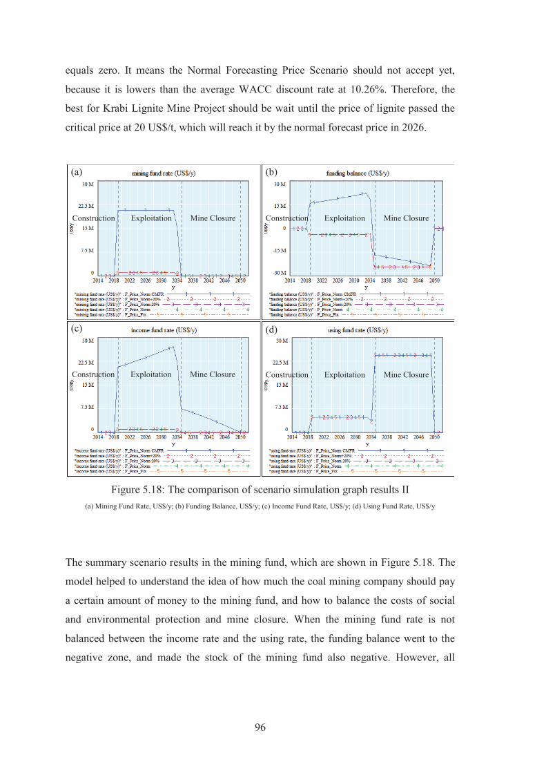
96
equals zero. It means the Normal Forecasting Price Scenario should not accept yet,
because it is lowers than the average WACC discount rate at 10.26%. Therefore, the
best for Krabi Lignite Mine Project should be wait until the price of lignite passed the
critical price at 20 US$/t, which will reach it by the normal forecast price in 2026.
Figure 5.18: The comparison of scenario simulation graph results II
(a) Mining Fund Rate, US$/y; (b) Funding Balance, US$/y; (c) Income Fund Rate, US$/y; (d) Using Fund Rate, US$/y
The summary scenario results in the mining fund, which are shown in Figure 5.18. The
model helped to understand the idea of how much the coal mining company should pay
a certain amount of money to the mining fund, and how to balance the costs of social
and environmental protection and mine closure. When the mining fund rate is not
balanced between the income rate and the using rate, the funding balance went to the
negative zone, and made the stock of the mining fund also negative. However, all
(a) (b)
(c) (d)
Exploitation Mine Closure Construction Exploitation Mine Closure Construction
Exploitation Mine Closure Construction Exploitation Mine Closure Construction
97
mining fund debt would be eventually balanced in the criterion variables of Net Cash
Balance and NPV Balance.
If the Krabi Lignite Mine Project pays only 0.13 US$/t, the mining fund will have an
income around 0.99 M US$/y, but the cost of social and environmental protection
should be 4.8 M US$/y, and mine closure costs should be 24.34 US$/y. It makes the
total debt of mining fund around -425.64 M US$. On the other hand, if the project is
decided to pay in an optimum rate, which is 2.71 US$/t, the fund will receive 20.67 M
US$ annually. Then, the cumulative mining fund will grow up to approximately 302 M
US$ in 2035, before, decreasing to zero (ideal) at the end of mine closure, which is
enough to pay for the closure period until the end of mine life.
Figure 5.19: The comparison of scenario simulation graph results III
(a) Coal Reserves, t; (b) Coal Production Rate, t/y; (c) Total Mining Period, dmnl; (d) Overburden Rate, m3/y
(a) (b)
(c) (d)
Exploitation Mine Closure Construction Exploitation Mine Closure Construction
Exploitation Mine Closure Construction Exploitation Mine Closure Construction
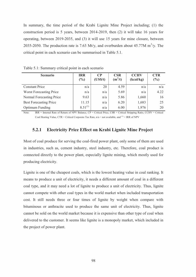
98
In summary, the time period of the Krabi Lignite Mine Project including; (1) the
construction period is 5 years, between 2014-2019, then (2) it will take 16 years for
operating, between 2019-2035, and (3) it will use 15 years for mine closure, between
2035-2050. The production rate is 7.63 Mt/y, and overburden about 45.77M m3/y. The
critical point in each scenario can be summarised in Table 5.1.
Table 5.1: Summary critical point in each scenario
Scenario IRR (%)
CP (US$/t)
CSR (m3/t)
CCHV (kcal/kg)
CTR (%)
Constant Price n/a 20 4.59 n/a n/a Worst Forecasting Price n/a n/a 5.69 n/a 4.22 Normal Forecasting Price 9.63 n/a 5.86 1,660 16 Best Forecasting Price 11.15 n/a 6.20 1,683 25 Optimum Funding 8.51(1) n/a 6.00 1,976 20 Note: IRR = Internal Rate of Return of NPV Balance, CP = Critical Price, CSR = Critical Stripping Ratio, CCHV = Critical
Coal Heating Value, CTR = Critical Corporate Tax Rate, n/a = not available, and (1) = IRR of NPV
5.2.1 Electricity Price Effect on Krabi Lignite Mine Project
Most of coal produce for serving the coal-fired power plant, only some of them are used
in industries, such as, cement industry, steel industry, etc. Therefore, coal product is
connected directly to the power plant, especially lignite mining, which mostly used for
producing electricity.
Lignite is one of the cheapest coals, which is the lowest heating value in coal ranking. It
means to produce a unit of electricity, it needs a different amount of coal in a different
coal type, and it may need a lot of lignite to produce a unit of electricity. Thus, lignite
cannot compete with other coal types in the world market when included transportation
cost. It still needs three or four times of lignite by weight when compare with
bituminous or anthracite used to produce the same unit of electricity. Thus, lignite
cannot be sold on the world market because it is expensive than other type of coal when
delivered to the customer. It seems like lignite is a monopoly market, which included in
the project of power plant.
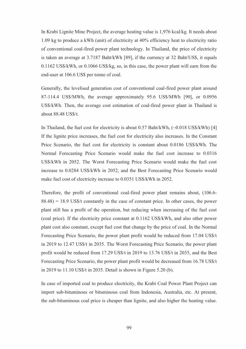
99
In Krabi Lignite Mine Project, the average heating value is 1,976 kcal/kg. It needs about
1.09 kg to produce a kWh (unit) of electricity at 40% efficiency heat to electricity ratio
of conventional coal-fired power plant technology. In Thailand, the price of electricity
is taken an average at 3.7187 Baht/kWh [89], if the currency at 32 Baht/US$, it equals
0.1162 US$/kWh, or 0.1066 US$/kg, so, in this case, the power plant will earn from the
end-user at 106.6 US$ per tonne of coal.
Generally, the levelised generation cost of conventional coal-fired power plant around
87-114.4 US$/MWh, the average approximately 95.6 US$/MWh [90], or 0.0956
US$/kWh. Then, the average cost estimation of coal-fired power plant in Thailand is
about 88.48 US$/t.
In Thailand, the fuel cost for electricity is about 0.57 Baht/kWh, (~0.018 US$/kWh) [4]
If the lignite price increases, the fuel cost for electricity also increases. In the Constant
Price Scenario, the fuel cost for electricity is constant about 0.0186 US$/kWh. The
Normal Forecasting Price Scenario would make the fuel cost increase to 0.0316
US$/kWh in 2052. The Worst Forecasting Price Scenario would make the fuel cost
increase to 0.0284 US$/kWh in 2052, and the Best Forecasting Price Scenario would
make fuel cost of electricity increase to 0.0351 US$/kWh in 2052.
Therefore, the profit of conventional coal-fired power plant remains about, (106.6-
88.48) = 18.9 US$/t constantly in the case of constant price. In other cases, the power
plant still has a profit of the operation, but reducing when increasing of the fuel cost
(coal price). If the electricity price constant at 0.1162 US$/kWh, and also other power
plant cost also constant, except fuel cost that change by the price of coal. In the Normal
Forecasting Price Scenario, the power plant profit would be reduced from 17.04 US$/t
in 2019 to 12.47 US$/t in 2035. The Worst Forecasting Price Scenario, the power plant
profit would be reduced from 17.29 US$/t in 2019 to 13.76 US$/t in 2035, and the Best
Forecasting Price Scenario, the power plant profit would be decreased from 16.78 US$/t
in 2019 to 11.10 US$/t in 2035. Detail is shown in Figure 5.20 (b).
In case of imported coal to produce electricity, the Krabi Coal Power Plant Project can
import sub-bituminous or bituminous coal from Indonesia, Australia, etc. At present,
the sub-bituminous coal price is cheaper than lignite, and also higher the heating value.

100
Sub-bituminous coal, export of Indonesia has a heating value around 4,100 – 5,200
kcal/kg, an average of 4,650 kcal/kg [91]. The FOB Kalimantan price of coal is 38.5
US$/t at 4,200 kcal/kg [92]. Therefore, in the constant imported coal price, the profit of
the power plant will reach 36.67 US$/t. It is still 17.77 US$/t higher than using
domestic coal at Krabi.
(a) Unit of Power Plant Fuel Cost, US$/kWh; (b) Unit Power Plant Profit, US$/t
Figure 5.20: Krabi power plant decision condition
In summary, the Krabi Coal Power Plant Project can get profit by importing coal rather
than using domestic coal. If the criterion of the Krabi Power Plant Project is a maximum
profit, the decision on imported coal is chosen. However, the Krabi Lignite Mine
Project can provide a lower risk of supply chain, the new jobs, and economics of the
country, which is discussed in the next section.
5.2.2 Economic Value of Krabi Lignite Mine Project
Mining project and other business always serve parts of economics, (1) economics of
the project, and (2) economics of the society. Firstly, the economics of the mining
project should be profitable. In case of the Krabi Lignite Mine Project, the completely
return to profit is only the Best Forecasting Price Scenario, which will not easily happen
in the condition, because of the lignite price growth higher 20% of the normal
forecasting price trend. In additions, the Normal Forecasting Price Scenario goes to
profit if IRR is 8.51% in optimum mining fund rate condition, while the average
(a) (b)
Exploitation Mine Closure Construction
Exploitation Mine Closure Construction
101
discount rate of Thailand estimated at 10.26%. That is a reason why this project should
not operate at this moment.
On the other hand, the indirect activity of the area, which happen by the mining project.
It is also the economic value of society. First is the job opportunity of the area. The
Krabi Lignite Mine Project can create 852 jobs, which including 613 miners, 155
service supporters, and 84 technicians and administrative staffs. The 852 jobs mean 852
families have direct money from the mine to serve their life, which they can pay for
goods and services in the area, and also taxes on everyday life. It creates more and more
indirect jobs to support the society.
Second is the Royalty and Corporate tax paid by the mining project. It is approximately
97.68 M US$ of royalties and 83.91 M US$ of corporate tax in the operating period.
This part of the money can also motivate the economics of community in the area and
the big picture of Thailand such as, infrastructure system, school, hospital, road, bridge,
etc. Detail of optimum mining fund rate scenario is shown in Figure 5.21.
(a) Royalties Received, US$; (b) Corporate Tax Received, US$
Figure 5.21: Economic value of society by royalties and corporate tax
Moreover, by the new decision criteria of NPV Balance with mining fund, which
support social and environmental protection and mine closure. It should be better that
the society and the community nearby the mine have more guaranteed to protect the
environment and quality of life. It gains approximately 302.03 M US$ along period of
(a) (b)
Exploitation Mine Closure Construction Exploitation Mine Closure Construction
102
mine life until mine closure completely. It creates direct jobs to support the activities,
and also indirect jobs of goods and services, and taxes.
Finally, the economic value of the Krabi Lignite Mine Project not only direct money
received from the mining project. Also indirect jobs, goods, and services provide for
supporting mining activities. Taxes and royalties also motivate the society in the area
and a bigger part. In addition, the mining fund support activities of social and
environmental protection and mine closure, which makes longer the economic value of
the area until the end of the mine closure period.
Therefore, if the Krabi Lignite Mine Project results in positive value, the Krabi Coal
Power Plant Project should be operated by using the domestic lignite in Krabi because
of the lower risk of supply chain and economic value of the society. However, it should
be done when the lignite price grows more than 20 US$/t which may reach this price in
2026. It also should think about the underground mining method or others in the
technical and cost of operation.
5.2.3 The Alternative of Krabi Coal Power Plant Project
As mentioned for the 800 MW coal power plant of Krabi. There are two possible fuel
sources. First is the lignite domestic reserves. The second choice is to use imported coal
from Indonesia, Australia, and etc. Because of the new decision criteria of the project
are proposed. Which is the NPV Balance and the Net Cash Balance, it makes mining
project in the future more secure, but also more costly for social and environmental
protection cost and mine closure cost. The mining fund helps to reduce the cost by
funding interest rate. It is one of the keys for sustainability of mining and society.
Using the domestic coal in Krabi in term of economics of the project is not suitable at
this moment. The simulation scenarios show the possible return to profit is only in the
Best Forecasting Price Scenario, while the Normal Forecasting Price Scenario can
succeed only if the IRR of the project is reduced to 8.51%, (average discount rate at
10.26%). The optimum funding rate is approximately 2.71 US$/t, which makes mining
fund enough money to use until the end of the mine closure period. This is the critical

103
point of the new decision criteria for accepting the project in the normal coal price
forecasting case.
In case of operating Krabi Lignite Mine with the optimum mining fund rate, the
economic value of the project has been mentioned before, such as the new jobs, it is
approximately 852 staffs and workers in the mine. The indirect jobs also created in the
community nearby the mine to support goods and services. The royalties and tax from
mine are estimated to be about 97.68 M US$ and 83.91 M US$ respectively, which can
support the infrastructure and the quality of life of the society. The activities are
supported by the mining fund about 302.03 M US$ also increases the economic value of
community nearby the mine and country.
When comparing with the importing coal, the price of importing coal always expensive
than domestic coal at the same type, because it includes the transportation cost. In case
of lignite, it cannot transport to compete with other types of coal because the lower
heating value makes more lignite required than other coal type at the same electricity
producing, detail is shown in Figure 5.22.
(a) Unit of Power Plant Fuel Cost, US$/kWh; (b) Unit Power Plant Profit, US$/t
Figure 5.22: Unit of power plant fuel cost and profit comparison
At the electricity price of 0.1162 US$/kWh in Thailand, using the domestic lignite can
make profit about 18.27 US$/t, while using the imported coal will make more profit
(36.67 US$/t). Therefore, if making a decision on the profit of the power plant project,
(a) (b)
Exploitation Mine Closure Construction Exploitation Mine Closure Construction

104
the Krabi Coal Power Plant Project should choose the imported coal, details are shown
in Table 5.2.
Table 5.2: Summary alternative of Krabi Coal Power Plant Project
Items Domestic coal Imported coal Power plant capacity (MW) 800 800 Coal heating value (kcal/kg) 1,976 4,200 Production required (Mt/y) 7.63 3.59 Coal price (US$/t) 17.1 38.5 (1)
Unit of coal required (kg/kWh) 1.089 0.512 Power plant fuel cost (US$/kWh) 0.0186 0.0197 Price of electricity (US$/kWh) 0.1162 0.1162 Power plant profit (US$/t) 18.27 36.67 (1) Price included transportation cost
Despite the price of coal importing increases at the normal forecasting rate, 1.4%, which
makes profit of power plant decrease faster than the domestic lignite. It is still higher
profit per tonne than using the domestic lignite; see graph (b) line number 1 and 3 in
Figure 5.22.
Therefore, the best choice of Krabi Coal Power Plant Project is the using of imported
coal for operating the power plant than the using domestic lignite in Krabi at this
moment. Furthermore, the best alternative of the Krabi Lignite Mine Project is the
lignite price over 20 US$/t, which may reach this value in 2026 by normal forecasting
price as mentioned above.

105
6 DEVELOPMENT OF APPLICATION INTERFACE
The development results in the form of the system dynamics model structure, see details
in Section 3.2.2 (p. 32) and relationship equations, see details in the Appendix 3 (p.
173), are hardly of use for the general end user. Therefore, the step of converting the
SDM to the application software for easier use and worldwide publishing is proposed.
However, the application in this version, (version 1.0), is the free trial version, so it is
not a full option connecting with the model's ability. It is developed to support two
types of simulation; (1) scenario simulation and (2) sensitivity analysis simulation. The
details of the application interface development are explained below.
Firstly, the user interface is developed. The user interface can be separated into three
groups, (1) general information forms, (2) the input forms, and (3) the result forms.
Then, the link between the user interface form and model structure is made by
connecting tool boxes in the form with the variables in the model. Finally, came
converting the user interface forms, the model structures, and other supported files, into
a Vensim package file.
Generally, the Vensim package file cannot be opened on the Vensim Reader Software,
which is free license software from Ventana System Inc. However, the end user must
download and install the Vensim Reader, on to their own computer, before it can open
the Vensim package file. This is still overly cumbersome for the general end user, who
may only have the Vensim package file and be unable to open it because the computer
does not have the Vensim Reader.
Therefore, in this thesis the Vensim Reader and The Vensim package file are converted
to a portable application by using free software for making portable applications. The
end result became the decision support system of coal mine planning version 1.0 (DSS-
CMPv1.0), which runs on Windows OS without the need for installation. The details of
the application interface result and how to use it, are explained in the next section.

106
6.1 Application Interface Result
Application Interface Diagram
The interface diagram for the application design for a simple and easy to understand
how to use the application is shown in the Figure 6.1.
Figure 6.1: Interface Diagram of DSS-CMPv1.0
Cover
Acknowledgements
Main Menu
Scenario Simulation Menu
Start
Sensitivity Analysis Simulation Menu
Scenario Simulation Condition Setup
Sensitivity Analysis Condition Setup
Scenario Results Sensitivity Analysis Results
ExitUser Manual

107
The decision support system of coal mine planning version 1.0 (DSS-CMPv1.0) is
developed to be a decision making tool for surface coal mine planning projects, which
specifically use the truck and shovel transportation system. The application starts with
the general information cover form (Figure 6.2), and then the acknowledgement form
(Figure 6.3), which holds information important to the developers.
For more information on how to use it, see the Application User Manual in the main
menu of the application.
Figure 6.2: Cover Interface of DSS-CMPv1.0
Figure 6.3: Acknowledgements Interface of DSS-CMPv1.0
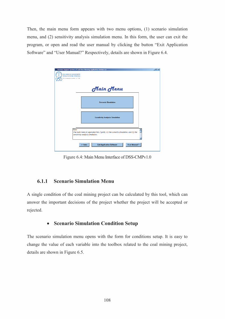
108
Then, the main menu form appears with two menu options, (1) scenario simulation
menu, and (2) sensitivity analysis simulation menu. In this form, the user can exit the
program, or open and read the user manual by clicking the button “Exit Application
Software” and “User Manual?” Respectively, details are shown in Figure 6.4.
Figure 6.4: Main Menu Interface of DSS-CMPv1.0
6.1.1 Scenario Simulation Menu
A single condition of the coal mining project can be calculated by this tool, which can
answer the important decisions of the project whether the project will be accepted or
rejected.
Scenario Simulation Condition Setup
The scenario simulation menu opens with the form for conditions setup. It is easy to
change the value of each variable into the toolbox related to the coal mining project,
details are shown in Figure 6.5.
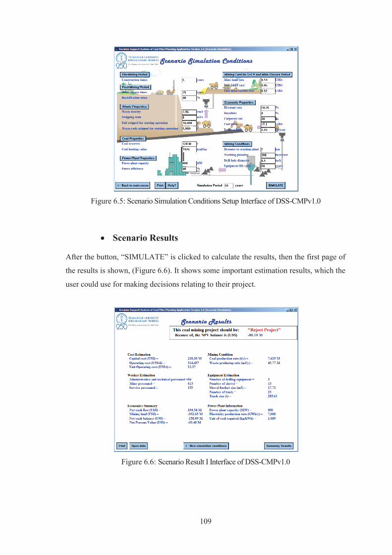
109
Figure 6.5: Scenario Simulation Conditions Setup Interface of DSS-CMPv1.0
Scenario Results
After the button, “SIMULATE” is clicked to calculate the results, then the first page of
the results is shown, (Figure 6.6). It shows some important estimation results, which the
user could use for making decisions relating to their project.
Figure 6.6: Scenario Result I Interface of DSS-CMPv1.0

110
Then, the end user can click “Summary Results” to review further details in comparison
graph, (Figure 6.7).
Figure 6.7: Scenario Result II Interface of DSS-CMPv1.0
Moreover, the application can also show the result in the form of table, see Figure 6.8.
Figure 6.8: Scenario Result III Interface of DSS-CMPv1.0
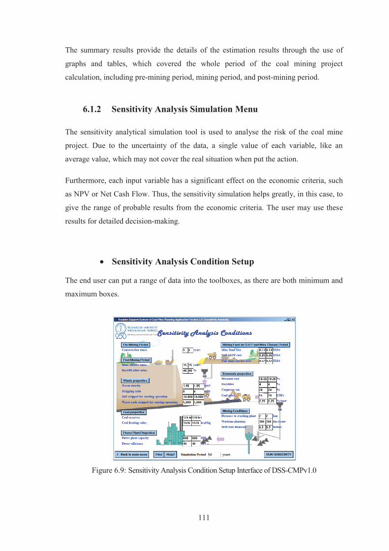
111
The summary results provide the details of the estimation results through the use of
graphs and tables, which covered the whole period of the coal mining project
calculation, including pre-mining period, mining period, and post-mining period.
6.1.2 Sensitivity Analysis Simulation Menu
The sensitivity analytical simulation tool is used to analyse the risk of the coal mine
project. Due to the uncertainty of the data, a single value of each variable, like an
average value, which may not cover the real situation when put the action.
Furthermore, each input variable has a significant effect on the economic criteria, such
as NPV or Net Cash Flow. Thus, the sensitivity simulation helps greatly, in this case, to
give the range of probable results from the economic criteria. The user may use these
results for detailed decision-making.
Sensitivity Analysis Condition Setup
The end user can put a range of data into the toolboxes, as there are both minimum and
maximum boxes.
Figure 6.9: Sensitivity Analysis Condition Setup Interface of DSS-CMPv1.0
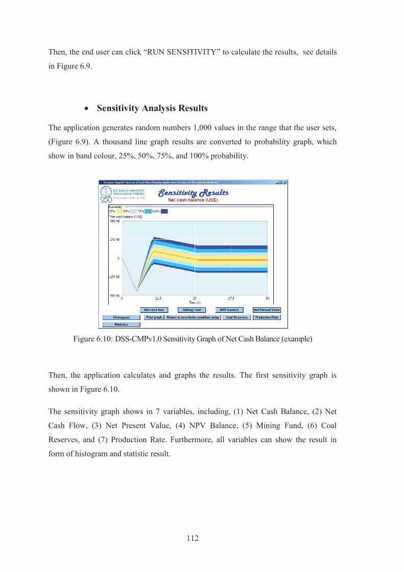
112
Then, the end user can click “RUN SENSITIVITY” to calculate the results, see details
in Figure 6.9.
Sensitivity Analysis Results
The application generates random numbers 1,000 values in the range that the user sets,
(Figure 6.9). A thousand line graph results are converted to probability graph, which
show in band colour, 25%, 50%, 75%, and 100% probability.
Figure 6.10: DSS-CMPv1.0 Sensitivity Graph of Net Cash Balance (example)
Then, the application calculates and graphs the results. The first sensitivity graph is
shown in Figure 6.10.
The sensitivity graph shows in 7 variables, including, (1) Net Cash Balance, (2) Net
Cash Flow, (3) Net Present Value, (4) NPV Balance, (5) Mining Fund, (6) Coal
Reserves, and (7) Production Rate. Furthermore, all variables can show the result in
form of histogram and statistic result.

113
Figure 6.11: DSS-CMPv1.0 Sensitivity Graph of NPV Balance (example)
Moreover, the use of the yellow band on the sensitivity graph to the end user is great.
They can see the black/red line graph as an average value of sensitivity result, which
helps them to understand the average result, and is crucial to the final decision on the
coal mining project, (Figure 6.11).
Figure 6.12: DSS-CMPv1.0 Sensitivity Graph of Cumulative Mining Fund (example)
114
The sensitivity of mining fund condition also can check with this application, which
means, in a constant mining fund rate, the uncertainty of other variables can make the
mining fund has widely value; detail is shown in Figure 6.12.
For more information such as, the detail of the results and the explanation of how to use
the application is shown in The Application User Manual, which can read in the
application main menu.
6.2 Application Installation and Usage
The decision support system of coal mine planning version 1.0 (DSS-CMPv1.0) is
developed by Vensim Software DSS version. The end user has 2 ways to use this
application. At first, the thesis model that developed in Vensim DSS, is made to be an
application package in “.vpa” extension, (DSS-CMPv1.0.vpa). This file can be run with
the Vensim Reader Software, which is free to download and install on a computer.
Thus, if the end user installs the Vensim Reader Software firstly, and then run the file
“DSS-CMPv1.0.vpa”, it is the first way to use this application.
However, in the second way, because of it still has two steps before the end user can use
the application including; (1) the end user must install the Vensim Reader Software on
their computer, and then, (2) runs the file “DSS-CMPv1.0.vpa”. This may constrain and
confuse the user, causing them to utilise the application only seldom.
Therefore, The “DSS-CMPv1.0_Portable.exe” is made by integrating the Vensim
Reader Software and the file model package “DSS-CMPv1.0.vpa”, which help the end
user can run the application without installation on a computer. It also has the
possibility to run the application directly on a handy drive. Finally, it is checked for
compatibility with Windows OS.
In addition, the application has a password protection. The password form is shown
when running the program, Figure 6.13.

115
Figure 6.13: Application password protection
The password for this version is “tufreiberg”, which can be accessed to the application.
If the wrong password is put, the blank application form will be shown, which the end
user cannot do anything.
Finally, this application version is a free trial version, which is published in order to
finish the PhD study and check the feedback of the application for further development.
The idea in the future is to make a commercial version and using the tool for consulting
of new mining project in Thailand.

116
7 SUMMARY AND RECOMMENDATION
7.1 Summary
The objectives of this thesis are, firstly is to develop the decision support system of a
coal mine planning tool by using the new modelling technique, calls system dynamics
model. Then, verify and validate with the real data of Mae Moh Lignite Mine. After
that, use the decision support system tool, which is developed in the first objective,
based upon the case study of the Krabi Lignite Mine Project for understanding situation
of this project.
Finally, the model that is developed in this thesis is converted to computer software,
which can be run on any version of Windows operating system. It is designed to be a
portable application that required no installation and could be run anywhere, no matter
from a hard disk or hard drive. The application is made to be user friendly in its
graphics and form. The confusing and complicating SDM structures and equations are
left out. It also included a user manual and hints for explanation. This application
software is the free trial version, which supported two important simulations. First is a
scenario simulation, which helps to analyse a single condition and give the details of
results, which included the suggestion to accept or reject the coal mining project,
graphs, and tables of the results. The second part is a sensitivity simulation, which is
helpful for deeper analysis and understanding of the probability results of the single or
combination of uncertain input data. It shows the result of calculation in a clear graphic
banding graph of probability result, and also in histograms and summary statistic values
at the end of the simulation period.
The decision-making on the case study in this thesis, Krabi Lignite Mine Project,
proposes two alternatives for Thailand; (1) to use domestic coal resources or (2)
imported coal from other countries. The developed SDM of this thesis helps clearly to
understand the situation of using the domestic coal resources in Krabi, which, despite
the approximate 120 Mt of lignite, is not suitable at this moment. Although, some
scenario simulation results, like the Best Forecasting Price positive results, may need
detailed analysis of the risk and likelihood. Furthermore, the optimum point of the
mining fund rate can also be found in the Normal Forecasting Price Scenario, which is
117
2.71 US$/t of production to maintain the mining fund in the positive value during mine
life at IRR 8.51%. However, the scenario results, which used the forecasting coal price
trend, the range of the real statistic data, such as data from the Mae Moh Lignite Mine,
Krabi Lignite Mine, and data on the Thai economics status, show significant results that
if the mining fund balance is included, the Krabi Lignite Mine Project may not suitable
at this time. The negative Net Cash Balance and NPV Balance mean it will not return a
profit on the investment at the end of mine life. The Krabi Lignite Mine Project should
wait until the lignite price goes up for more than 20 US$/t, which may already in 2026
by forecasting with normal trend of price.
7.2 Recommendations for Further Research
This work successfully reached the thesis objectives, which were developed the
decision support system of coal mine planning as an alternative user friendly application
software, and answering the case study of the Krabi Lignite Mine Project. However, the
boundary of the model structure, which focused on surface coal mining and specifically
the use of truck and shovel, can be extended to cover other equipment, such as
underground coal mining. Furthermore, the application of this example to other cases of
mining, such as metal mining, which bears specific processing requirements such as
grinding, chemical processing, and metallurgy, etc., or in quarrying, would also pose an
interesting challenge and can be continued hereafter. The underground mining also can
apply from this model by adjusting some variables; add some relationship and
equations, which can be done in the future development.
This example concentrates on the new coal mining project, to answer if the project
should be accepted or rejected, by using the criteria mining fund, which ensures
spending on social and environmental security and mine closure. However, on the
further development of the model, the detail of estimation of social and environmental
protection and mine closure cost, activity variables, and alternatives variables, which
did not have in this model, can be extended. Moreover, the development of each part of
the mine production planning, which are interconnected such as the blasting
management model [29-30], the transportation management model, the crushing and

118
processing management model, the equipment selection model, etc., can be continued in
the future.
The policy decision on the sustainability of mining and the environment in each area
and condition can explain and find the suitable solution and continue by extracting and
extending part of mining fund. In addition, a small-scale mining solution can be
continuing adapted and extended from the economic model of this thesis in the future.
Finally, further research could be focused on, the automatic or real-time, responding of
decision-making tools, by integrating the technology of measurement or sensor
detection. The data results from the measuring devices can be automatically transferred
the values into the model whilst continuing the process and making a decision.

119
REFERENCES [1] R. Heinberg and D. Fridley. (2011, The End of Cheap Coal. Available:
http://www.postcarbon.org/article/406162-the-end-of-cheap-coal [2] Wikipedia.org. (2012, 28 August). Coal. Available:
http://en.wikipedia.org/wiki/Coal [3] EGAT. (2014, 5 April). Mae Moh Power Plant. Available:
http://www.egat.co.th/images/information/plants-info/maemoh.pdf [4] A. Kittichotkul, "Mae Moh Lignite Mining 2011: PowerPoint Presentation,"
Electricity Generating Authority of Thailand (EGAT)2011. [5] P. Chumrum, et al., Coal Mining Technology: Electricity Generating Authority
of Thailand: EGAT, 1995. [6] C. Drebenstedt, "Responsible Mining - Approaches and Realization," in 22nd
World Mining Congress & Expo 2011, Istanbul, 2011, p. 135. [7] C. Roumpos, et al., "A Decision Making Model for Lignite Deposits
Exploitability," in Mine Planning and Equipment Selection 2004, Wroclaw, Poland, 2004, pp. 721-726.
[8] Ventana System Inc. (2011, 28 May). Vensim Software. Available: http://www.vensim.com/software.html
[9] Wikipedia.org. (2011, 28 February). Net present value. Available: http://en.wikipedia.org/wiki/Net_present_value
[10] Wikipedia.org. (2014, 5 March). Payback period. Available: http://en.wikipedia.org/wiki/Payback_period
[11] Z. Bian, et al., "Environmental issues from coal mining and their solutions," Mining Science and Technology (China), vol. 20, pp. 215-223, 2010.
[12] BP, "BP Statistical Review of World Energy," 2014. [13] BP, "BP Statistical Review of World Energy," 2013. [14] EGAT, "Thailand Electricity Energy Status," Electricity Generating Authority of
Thailand (EGAT)2012. [15] D. Katoria, et al., "Environment Impact Assessment of Coal Mining,"
International Journal of Environmental Engineering and Management, vol. 4, pp. 245-250, 2013.
[16] C. Drebenstedt, "Conditions for Mine Closure Strategy in Great European Coal Mine," in Mine Closure 2006: Proceeding of the First International Seminar on Mine Closure, Perth, Australia, 2006, pp. 117-129.
[17] Wikipedia.org. (2011, 15 February). System dynamics. Available: http://en.wikipedia.org/wiki/System_dynamics
[18] BEP, "Coal mining process," miningprocessnew-large.jpg, Ed., ed: PT. Bhakti Energi Persada, 2011.
[19] EGAT. (2013, 10 January). About us. Available: http://maemohmine.egat.co.th/aboutus/index.html
[20] PeopleVoice. (2013, 5 April). Krabi Power Plant. Available: http://www.ppvoice.org/?p=2873
[21] EIA. (2013, Use of coal. Available: http://www.eia.gov/energyexplained/index.cfm?page=coal_use
[22] EIA. (2013, How much coal is left. Available: http://www.eia.gov/energyexplained/index.cfm?page=coal_reserves

120
[23] E. Britannica. (2011, 22 February). Coal (fossil fuel). Available: http://www.britannica.com/EBchecked/topic/122863/coal
[24] E. Britannica. (2011, 31 May). coal: occurrences on Earth. Available: http://www.britannica.com/EBchecked/media/1625/Location-of-the-most-important-coal-occurrences-on-Earth
[25] E. Britannica. (2011, 22 February). Coal Mining. Available: http://www.britannica.com/EBchecked/topic/122975/coal-mining
[26] EIA. (2013, Coal Mining and Transportation. Available: http://www.eia.gov/energyexplained/index.cfm?page=coal_mining
[27] R. Mitra and S. Saydam. (2012, Surface Coal Mining Methods in Australia. 3-22. Available: http://cdn.intechopen.com/pdfs-wm/30795.pdf
[28] S. Bhandari, Engineering rock blasting operations. Rotterdam, Netherlands ; Brookfield, VT: A.A. Balkema, 1997.
[29] P. Sontamino and C. Drebenstedt, "A Prototype Dynamics Model of Bench Blasting Design," in The 10th International Conference on Mining, Materials and Petroleum Engineering, The 6th International Conference on Earth Resources Technology “Sciences and Technologies Towards 2012” : PSU-IC 2012, Songkhla, Thailand, 2012.
[30] P. Sontamino and C. Drebenstedt. (2012, A Dynamics Model of Surface Coal Blasting Design Pattern. Scientific Reports on Resource Issues 2012 1(2012), 98-107.
[31] J. P. Paul and M. Sengupta, "Computer aided blasting-round design in an arctic coal mine," Mining Science and Technology, vol. 5, pp. 299-308, 1987.
[32] B. Forbies, "Longwall Mining Method," vol. 692.9 kb, L. M. Actual.jpg, Ed., ed: flexsim.com, 2013.
[33] Wikipedia.org. (2014, 28 April). Coal. Available: http://en.wikipedia.org/wiki/Coal
[34] Wikipedia.org. (2014, 24 June). List of countries by coal production. Available: http://en.wikipedia.org/wiki/List_of_countries_by_coal_production
[35] EIA. (2013, Coal Prices and Outlook. Available: http://www.eia.gov/energyexplained/index.cfm?page=coal_prices
[36] EIA, "Annual Energy Review 2011," U.S. Energy Information Administration2011.
[37] EIA. (2014, International Energy Statistics: Coal Import. Available: http://www.eia.gov/cfapps/ipdbproject/iedindex3.cfm?tid=1&pid=1&aid=3&cid=regions&syid=2006&eyid=2012&unit=TST
[38] EIA. (2013, Coal Imports and Exports. Available: http://www.eia.gov/energyexplained/index.cfm?page=coal_imports
[39] EIA. (2014, International Energy Statistics: Coal Export. Available: http://www.eia.gov/cfapps/ipdbproject/iedindex3.cfm?tid=1&pid=1&aid=4&cid=regions&syid=2006&eyid=2012&unit=TST
[40] C. Drebenstedt, "Financial Valuation of Mine Closure Alternatives," in Mine Closure 2006: Proceeding of the First International Seminar on Mine Closure, Perth, Australia, 2006, pp. 499-508.
[41] EIA. (2013, Coal and the environment. Available: http://www.eia.gov/energyexplained/index.cfm?page=coal_environment
[42] P. Sontamino and C. Drebenstedt. (2013, A System Dynamics Model of Mining Cost Estimation. Scientific Reports on Resource Issues 2013 1(2013), 309-315.
121
[43] W. A. Hustrulid and M. Kuchta, Open pit mine planning & design. Rotterdam ; Brookfield, VT: A.A. Balkema, 1998.
[44] W. A. Hustrulid and M. Kuchta, Open pit mine planning & design, 2 ed.: Taylor & Francis, 2006.
[45] A. H. Watson, "Better Closure Cost Estimates," in Mine Closure 2006: Proceeding of the First International Seminar on Mine Closure, Perth, Australia, 2006, pp. 493-497.
[46] L. Wilde, "Costs of Mine Closure-Learning from the Past," in Mine Closure 2007: Proceeding of the Second International Seminar on Mine Closure, Santiago, Chile, 2007, pp. 383-391.
[47] A. Peralta-Romero and K. Dagdelen, "A New Model for Estimation of Mine Closure Costs," in Mine Closure 2007: Proceeding of the Second International Seminar on Mine Closure, Santiago, Chile, 2007, pp. 393-404.
[48] I. M. Weiersbye, "Global Review and Cost Comparison of Conventional and Phytotechnologies for Mine Closure," in Mine Closure 2007: Proceeding of the Second International Seminar on Mine Closure, Santiago, Chile, 2007, pp. 13-30.
[49] P. Sontamino and C. Drebenstedt, "A Prototype Dynamics Decision Making Model of Mining Feasibility Study on Investment," in International Forum-Competition of Young Researches, St.Petersburg, 2013, pp. 76-79.
[50] M. Heidari and F. Rashidinejad, "Evaluation of Sungun Copper Mine Design," in Mine Planning and Equipment Selection 2004, Wroclaw, Poland, 2004, pp. 31-36.
[51] Wikipedia.org. (2011, 28 February). Internal rate of return. Available: http://en.wikipedia.org/wiki/Internal_rate_of_return
[52] J. Cech and V. Bauer, "A Computerized Evaluation of Mining Project," in Mine Planning and Equipment Selection 2004, Wroclaw, Poland, 2004, pp. 643-646.
[53] C. Drebenstedt and D. Slaby, "Valuation of Long-term Post-mining Activities," in Mine Planning and Equipment Selection 2004, Wroclaw, Poland, 2004, pp. 659-665.
[54] C. Drebenstedt, "Financial Valuation of Mining Remediation Objectives," in International Mining Conference: Advance Mining for Sustainable Development, Ha Long, Vietnam, 2010, pp. 30-40.
[55] L. A. Martin. The First Step [Online]. Available: http://ocw.mit.edu/courses/sloan-school-of-management/15-988-system-dynamics-self-study-fall-1998-spring-1999/readings/step.pdf
[56] Wikipedia.org. (2011, 23 February). Jay Wright Forrester. Available: http://en.wikipedia.org/wiki/Jay_W._Forrester
[57] E. Britannica. (2011, 23 February). Jay Wright Forrester. Available: http://www.britannica.com/EBchecked/topic/213987/Jay-Wright-Forrester
[58] Wikipedia.org. (2011, 28 February). The Limits to Growth. Available: http://en.wikipedia.org/wiki/The_Limits_to_Growth
[59] T. S. D. Society. (2011, 24 February). What is System Dynamics? Available: http://www.systemdynamics.org/what_is_system_dynamics.html
[60] Wikipedia.org. (2014, 6 March). List of system dynamics software. Available: http://en.wikipedia.org/wiki/List_of_system_dynamics_software
[61] P. M. Budzik and R. F. Naill, "FOSSIL1: A policy analysis model of the U.S. energy transition," presented at the Proceedings of the 76 Bicentennial conference on Winter simulation, Gaithersburg, MD, 1976.

122
[62] Y. Fan, et al., "A system dynamics based model for coal investment," Energy, vol. 32, pp. 898-905, 2007.
[63] A. Caselles-Moncho, et al., "Dynamic simulation model of a coal thermoelectric plant with a flue gas desulphurisation system," Energy Policy, vol. 34, pp. 3812-3826, 2006.
[64] B. O'Regan and R. Moles, "An insight into the system dynamics method: a case study in the dynamics of international minerals investment," Environmental Modelling & Software, vol. 16, pp. 339-350, 2001.
[65] DMR, "Map of Coal Resources and Reserves in Thailand," ed: Department of Mineral Resources of Thailand, 2003.
[66] EPPO, "Energy Statistics of Thailand 2012," Thailand Ministry of Energy Annual Report: 2012.
[67] EPPO, "Energy Statistics of Thailand 2013," Thailand Ministry of Energy Annual Report: 2013.
[68] GoogleMap. (2014, Mae Moh Lignite Mining Position. Available: https://www.google.de/maps/@18.3425068,99.720318,16977m/data=!3m1!1e3?hl=en
[69] Nay Zarlin, et al., "Numerical Study on an Applicable Underground Mining Method for Soft Extra-Thick Coal Seams in Thailand," Engineering, vol. 4, pp. 739-745, 22 September 2012.
[70] GoogleMap. (2014, Krabi Lignite Reserve Position. Available: https://maps.google.de/maps?q=7.997527,99.033752&hl=de&ll=7.988348,99.041662&spn=0.074713,0.077162&num=1&t=h&z=14
[71] EGAT. (2014, 5 April). Krabi Power Plant. Available: http://www.egat.co.th/images/information/plants-info/krabee_powerplant.pdf
[72] Thaipost. (2014, 5 April). EGAT believed, the new Krabi Power Plant will finish in 2019. Available: http://www.thaipost.net/news/110314/87281
[73] Wikipedia.org. (2014, 19 March). Exogeny. Available: http://en.wikipedia.org/wiki/Exogeny
[74] EPPO, "Summary of Thailand Power Development Plan 2012-2030," Thailand Ministry of Energy 2012.
[75] Wikipedia.org. (2014, 27 March). Kilowatt hour. Available: http://en.wikipedia.org/wiki/Kilowatt_hour
[76] WCA. (2014, Improving Efficiencies. Available: http://www.worldcoal.org/coal-the-environment/coal-use-the-environment/improving-efficiencies/
[77] Wikipedia.org. (2014, 1 April). Weighted average cost of capital. Available: http://en.wikipedia.org/wiki/Weighted_average_cost_of_capital
[78] B. McClure. (2009, 25 February). DCF Analysis: Calculating The Discount Rate. Available: http://www.investopedia.com/university/dcf/dcf3.asp
[79] I. C. Runge, Mining economics and strategy. Littleton, CO: Society for Mining, Metallurgy, and Exploration, 1998.
[80] Trading_Economics. (2014, Thailand Interest Rate. Available: http://www.tradingeconomics.com/thailand/interest-rate
[81] BOT. Interest Rates in Financial Market (2005- present) [Online]. Available: http://www.bot.or.th/English/Statistics/FinancialMarkets/InterestRate/Pages/StatInterestRate.aspx
[82] Trading_Economics. (2014, Thailand Inflation Rate. Available: http://www.tradingeconomics.com/thailand/inflation-cpi

123
[83] GDP_Inflation. (2014, Inflation Rate in Thailand (from1990 to 2014). Available: http://www.gdpinflation.com/2013/07/inflation-rate-in-thailand-from1990-to.html
[84] Trading_Economics. (2014, 1 April). Lending Interest Rate (%) In Thailand. Available: http://www.tradingeconomics.com/thailand/lending-interest-rate-percent-wb-data.html
[85] E. Topal, "Evaluation of a mining project using Discounted Cash Flow analysis, Decision Tree analysis, Monte Carlo Simulation and Real Options using an example," International Journal of Mining and Mineral Engineering, vol. 1, pp. 62-76, 2008.
[86] M. Osanloo and H. Hamidian, "OPCE-Software Developed for Cost Estimation of Mined Material in Open Pit Mine Based on O'Hara's Detailed and Escalation Methods," in Mine Planning and Equipment Selection 2004, Wroclaw, Poland, 2004, pp. 697-702.
[87] Ventana System Inc. (2014, 10 May). Vensim Help. Available: http://www.vensim.com/documentation/index.html?vensim_help.htm
[88] EIA. (2014, Annual Energy Outlook 2014. Available: http://www.eia.gov/forecasts/aeo/er/pdf/0383er(2014).pdf
[89] P. Ruangrong. (2012, Power Tariff Structure in Thailand. Available: http://www.eria.org/events/Power%20Tariff%20Structure%20in%20Thailand.pdf
[90] Wikipedia.org. (2014, 20 July). Cost of electricity by source. Available: http://en.wikipedia.org/wiki/Cost_of_electricity_by_source
[91] D. L. Ewart and R. Vaughn. (2009, Indonesian Coal. Available: http://www.marston.com/portals/0/marston_review_of_indonesian_thermal_coal_industry.pdf
[92] PlattsCoal. (2013, October 31). Coal Trader International. Available: http://www.platts.com/IM.Platts.Content/ProductsServices/Products/coaltraderintl.pdf
[93] AnyLogic. (2014, 30 December). Multimethod Simulation Approach. Available: http://www.anylogic.com/multimethod-modeling
[94] AnyLogic. (2014, 31 December). Use of Simulation Modeling. Available: http://www.anylogic.com/use-of-simulation

124
I. APPENDIX 1: BACKGROUND INFORMATION
Energy is one important key for the development of a country. Everyone consumes
energy in direct and indirect ways. A pound of coal provides enough electricity to
power ten (100 W) light bulbs for about an hour [21]. No one can estimate the exact
amount of coal deposits that remain around the world; There is an idea of coal proved
reserves, coal resources, identified or discovered coal resources, and total coal resources
appearing like a shape of pyramid [22]. The example of the coal reserves and resources
pyramid from the USA is shown in the Figure I.1 below.
Figure I.1: Pyramid of the USA coal resources and reserves [22]
World Coal Status and Coal Mining
General Coal History and Classification
Coal classification can be separated into many system types. The different varieties of
coal arise because of differences in the kinds of formation plant material (coal type),
degree of coalification (coal ranking), or the range of impurities (coal grade) [23].
However, the ranking of degree of coalification and metamorphism is a traditional
125
classification of coal. This method separated coal types into two groups, (1) High rank
coal, and (2) Low rank coal [5]. As geological processes apply heat and pressure to the
deadly biotic material over time, and under the appropriate conditions, it is transformed
successively into [2]:
(1) Peat: considered to be a precursor of coal, it has industrial importance as a fuel
in some regions. In its dehydrated form, peat is a highly effective absorbent for
fuel and oil spills on land and water. It is also used as a conditioner for soil to
make it more able to retain and slowly release water [2].
(2) Lignite: or brown coal, it is the lowest rank of coal and used almost exclusively
as fuel for electric power generation. A compact form of lignite is sometimes
polished, and it has been used as an ornamental stone [2].
(3) Sub-bituminous coal: the properties range between lignite to bituminous coal,
it is used primarily as fuel for steam-electric power generation, and it is an
important source of light aromatic hydrocarbons for the chemical synthesis
industry [2].
(4) Bituminous coal: it is a dense sedimentary rock, usually black, but sometimes
dark brown, often with well-defined bands of bright and dull material; it is used
primarily as fuel in steam-electric power generation, with substantial quantities
used for heat and power applications in manufacturing and to make coke [2].
(5) Steam coal: it is a grade between bituminous coal and anthracite, once widely
used as a fuel for steam locomotives. In this specialized use, it is sometime
known as “sea-coal” in the US. Small steam coal (dry small steam nuts - DSSN)
is used as a fuel for domestic water heating [2].
(6) Anthracite: the highest rank of coal, it is a harder, glossy black coal used
primarily for residential and commercial space heating. It may be divided further
into metamorphically altered bituminous coal and “petrified oil”, as from the
deposits in Pennsylvania [2].
(7) Graphite: technically the highest rank, it is difficult to ignite, and is not
commonly used as fuel – it is mostly used in pencils and, when powdered, as a
lubricant [2].
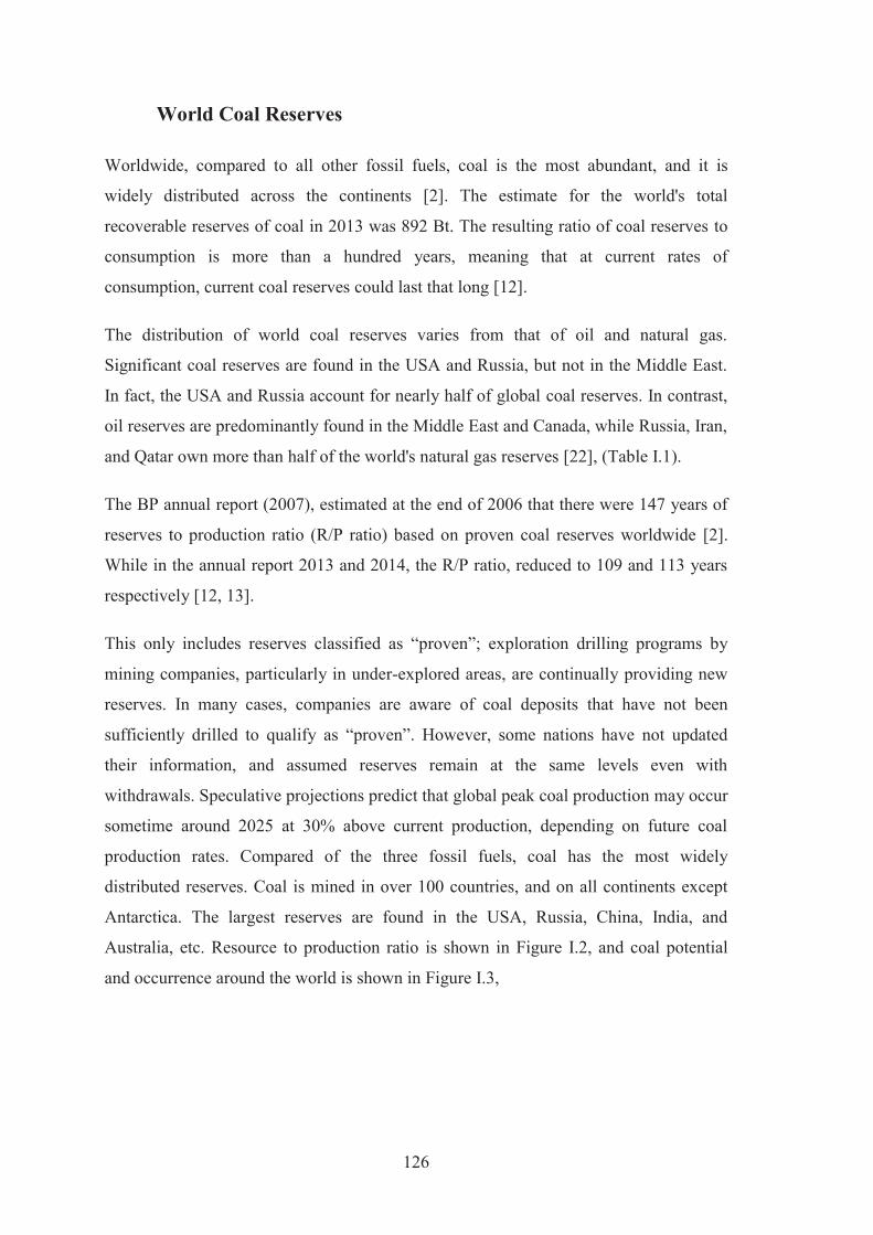
126
World Coal Reserves
Worldwide, compared to all other fossil fuels, coal is the most abundant, and it is
widely distributed across the continents [2]. The estimate for the world's total
recoverable reserves of coal in 2013 was 892 Bt. The resulting ratio of coal reserves to
consumption is more than a hundred years, meaning that at current rates of
consumption, current coal reserves could last that long [12].
The distribution of world coal reserves varies from that of oil and natural gas.
Significant coal reserves are found in the USA and Russia, but not in the Middle East.
In fact, the USA and Russia account for nearly half of global coal reserves. In contrast,
oil reserves are predominantly found in the Middle East and Canada, while Russia, Iran,
and Qatar own more than half of the world's natural gas reserves [22], (Table I.1).
The BP annual report (2007), estimated at the end of 2006 that there were 147 years of
reserves to production ratio (R/P ratio) based on proven coal reserves worldwide [2].
While in the annual report 2013 and 2014, the R/P ratio, reduced to 109 and 113 years
respectively [12, 13].
This only includes reserves classified as “proven”; exploration drilling programs by
mining companies, particularly in under-explored areas, are continually providing new
reserves. In many cases, companies are aware of coal deposits that have not been
sufficiently drilled to qualify as “proven”. However, some nations have not updated
their information, and assumed reserves remain at the same levels even with
withdrawals. Speculative projections predict that global peak coal production may occur
sometime around 2025 at 30% above current production, depending on future coal
production rates. Compared of the three fossil fuels, coal has the most widely
distributed reserves. Coal is mined in over 100 countries, and on all continents except
Antarctica. The largest reserves are found in the USA, Russia, China, India, and
Australia, etc. Resource to production ratio is shown in Figure I.2, and coal potential
and occurrence around the world is shown in Figure I.3,

127
Figure I.2: Resource to production ratio 2013 [12]
Moreover, the distribution of coal proved reserves is shown in Figure I.4.
Figure I.3: Coal potential and occurrence around the world [24]
53 years
55 years
113 years
Oil
Gas
Coal
Coal
Oil
Gas

128
Figure I.4: Distribution of proved reserves in 1992, 2002, and 2012 [13]
Table I.1: Top 5 world hydrocarbon energy reserves by country (2011) [22]
Coal Oil Natural Gas
USA 27.5% Saudi Arabia 17.7% Russia 25.2%
Russia 18.3% Venezuela 14.4% Iran 15.7%
China 13.3% Canada 11.9% Qatar 13.4%
Other Non-OECD
Europe and Eurasia
10.7% Iran 9.3% Saudi Arabia 4.1%
Others 30.2% Others 46.7% Others 41.6%
Total 100% Total 100% Total 100%
Source: The Energy Information Administration, International Energy Outlook, USA, September 2011.
Moreover, the top 5 of the world coal reserves (2013) is shown in the Table I.2.
Table I.2: Top 5 world coal reserves by countries (2013) [12]
Country Anthracite & Bituminous Sub-bituminous and Lignite Total % Share USA 108,501 128,794 237,295 26.6 Russia 49,088 107,922 157,010 17.6 China 62,200 52,300 114,500 12.8 Australia 37,100 39,300 76,400 8.6 India 56,100 4,500 60,600 6.8
World Total 403,199 488,332 891,531 100
Unit: Mt

129
Coal Mining System
Generally, Coal miners use giant machines to remove coal from the ground. They
actually use two methods: (1) surface mining, or (2) underground mining [25]. In the
USA, many coal beds are shallow, and about two-thirds of coal production come from
surface mines. Modern mining methods bring most coal reserves into easy reach. Due to
growth in surface mining and improved mining technology, the amount of coal
produced by a miner in an hour has more than tripled since 1978 [26].
Surface Coal Mining
Surface coal mining is used to produce most of the coal in the USA, and all around the
world, because it is cheaper than underground mining in terms of unit cost per tonne.
Usually, surface coal mining can be used when the coal is buried less than 60 m
underground [26], or when it is still economical to operate the surface mining method.
The most flexible method applied in surface coal mining is the truck and shovel
method, which can be utilised in different geological conditions [27].
Figure I.5: Surface coal mining method (example) [27]
In surface mining, giant machines, such as draglines and shovels, remove the topsoil
and layers of rock known as “overburden” to expose the coal seam below. Then, when
the mining is finished, the dirt and rock are returned to the pit, the topsoil is replaced,

130
and the area is replanted [26]. In some areas, which need blasting technique, such as
compact rock of overburden, bench blasting can be applied [28, 29]; specific coal
blasting can also be used for compact coal [30, 31].
Underground Coal Mining
Underground mining, sometimes called “deep mining”, is used when the coal is buried
several 30.5 m below the surface, and it is uneconomic to operate surface mining
methods. Some underground mines are 305 m deep. To remove coal in these
underground mines, miners ride lifts down deep mine shafts where they run machines
that dig out the coal [26]. The popular underground coal mining method is Longwall
Mining, which is suitable with horizontal coal seams.
Figure I.6: Longwall mining method [32]
Coal Processing
After coal comes out of the ground, it typically goes on a conveyor belt to a preparation
plant that is located at the mining site. The plant cleans and processes the coal to
remove other rocks, dirt, ash, sulphur, and unwanted materials, increasing the heating
value of the coal [26].
Coal Transportation
After the coal is mined and processed, it is ready to be shipped to market. The cost of
shipping coal can be more than the cost of mining it [26].
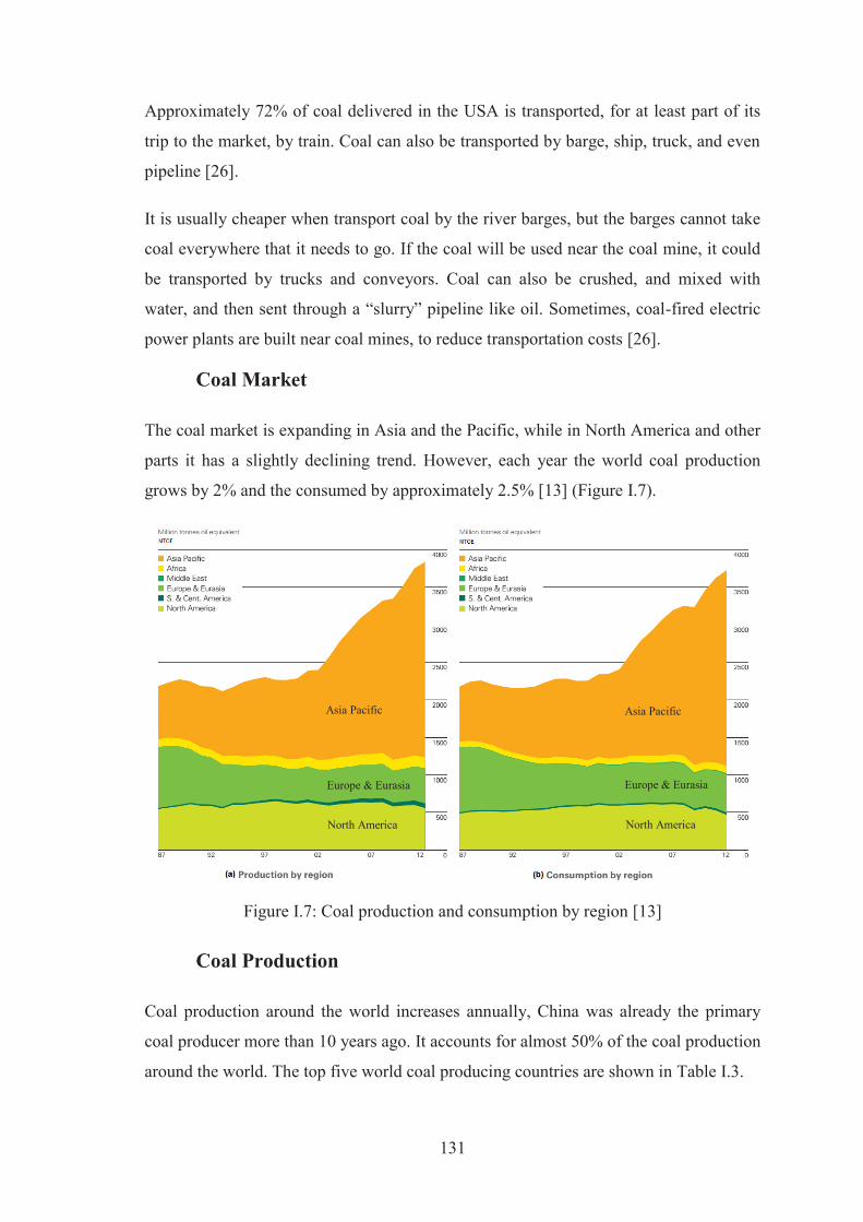
131
Approximately 72% of coal delivered in the USA is transported, for at least part of its
trip to the market, by train. Coal can also be transported by barge, ship, truck, and even
pipeline [26].
It is usually cheaper when transport coal by the river barges, but the barges cannot take
coal everywhere that it needs to go. If the coal will be used near the coal mine, it could
be transported by trucks and conveyors. Coal can also be crushed, and mixed with
water, and then sent through a “slurry” pipeline like oil. Sometimes, coal-fired electric
power plants are built near coal mines, to reduce transportation costs [26].
Coal Market
The coal market is expanding in Asia and the Pacific, while in North America and other
parts it has a slightly declining trend. However, each year the world coal production
grows by 2% and the consumed by approximately 2.5% [13] (Figure I.7).
Figure I.7: Coal production and consumption by region [13]
Coal Production
Coal production around the world increases annually, China was already the primary
coal producer more than 10 years ago. It accounts for almost 50% of the coal production
around the world. The top five world coal producing countries are shown in Table I.3.
Asia Pacific Asia Pacific
Europe & Eurasia Europe & Eurasia
North America North America

132
Table I.3: Top 5 world coal producers (2004-2012) [33, 34]
Country/Region 2004 2005 2006 2007 2008 2009 2010 2011 2012 China 2,123 2,350 2,529 2,692 2,802 2,973 3,235 3,520 3,650 USA 1,009 1,027 1,055 1,040 1,063 975 984 993 922 India 408 428 449 478 516 556 574 589 606 European Union 628 607 595 592 564 538 536 576 581 Australia 364 375 382 393 399 413 424 416 431
World Total 5,716 6,035 6,342 6,573 6,795 6,881 7,255 7,695 7,865 Unit: Mt
All of the coal production in China is used for domestic purposes, and China also
imports coal from other countries, which take the second position of the world coal
importing country, (Table I.6).
Coal Consumption
The trend of coal consumption is increasing, the main part which is consumed by the
Asia Pacific zone. China is not only the primary producer of the world; it still takes the
place of number one coal consumer. The top five world coal consuming countries are
presented in Table I.4 [12].
Table I.4: Top 5 world coal consumers (2008-2013) [12]
Country 2008 2009 2010 2011 2012 2013 China 1,369 1,471 1,610 1,761 1,856 1,925 USA 564 496 525 495 437 456 India 230 250 260 270 302 324 Japan 129 109 124 118 124 129 Russia 100 92 90 94 98 94
World Total 3,262 3,239 3,469 3,630 3,724 3,827 Unit: MTOE
However, when comparing coal consumption per capita, it is Kazakhstan, which ranks
highest and with a consumption of more than 1.5 TOE per person annually (2012),
(Figure I.8) [13].
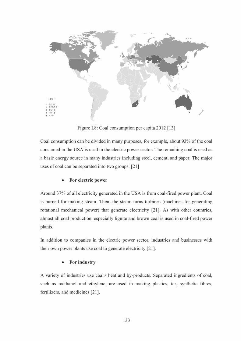
133
Figure I.8: Coal consumption per capita 2012 [13]
Coal consumption can be divided in many purposes, for example, about 93% of the coal
consumed in the USA is used in the electric power sector. The remaining coal is used as
a basic energy source in many industries including steel, cement, and paper. The major
uses of coal can be separated into two groups: [21]
For electric power
Around 37% of all electricity generated in the USA is from coal-fired power plant. Coal
is burned for making steam. Then, the steam turns turbines (machines for generating
rotational mechanical power) that generate electricity [21]. As with other countries,
almost all coal production, especially lignite and brown coal is used in coal-fired power
plants.
In addition to companies in the electric power sector, industries and businesses with
their own power plants use coal to generate electricity [21].
For industry
A variety of industries use coal's heat and by-products. Separated ingredients of coal,
such as methanol and ethylene, are used in making plastics, tar, synthetic fibres,
fertilizers, and medicines [21].
TOE

134
Coal is also used in the steel industry. At first, coal is baked in hot furnaces to make
coke. Then the coking coal is used to smelt iron ore into the iron, which needed for
making steel. It is the very high temperatures created from the use of coke that gives
steel the strength and flexibility for things like bridges, buildings, and cars.
Furthermore, the concrete and paper industries also use large amounts of coal [21].
Coal Prices
The price of coal varies by the coal ranking, mining method, geographic region, and
coal quality [35]. As previously stated, coal is generally classified into 4 main ranks
(lignite, sub-bituminous, bituminous, and anthracite), depending on the amounts and
types of carbon, which contains, and the amount of heat energy that can produce. Coals
with a high heating content are generally higher priced [35].
The average sales price, in 2011, of coal at mines producing, all of the four major ranks
of coal are shown in Table I.5 below [35],
Table I.5: Coal average sales prices (2011) [35]
Type Prices (US$/t)
Lignite 18.77
Sub-bituminous 14.07
Bituminous 68.50
Anthracite 75.70
Surface mined coal generally yields a lower price than underground coal mined. Where
coal beds are thick and near the surface, as in Wyoming (USA), mining costs and,
therefore, coal prices tend to be lower than where the beds are thinner and deeper, as in
Appalachia (USA). The higher cost of coal from underground mines reflects, in part, the
more difficult mining conditions and the need for more miners [35]. The history of
global coal price is shown in Figure I.9.
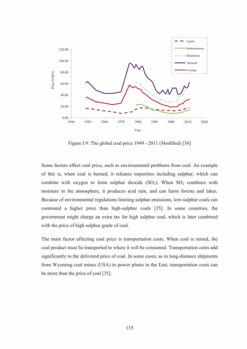
135
Figure I.9: The global coal price 1949 - 2011 (Modified) [36]
Some factors effect coal price, such as environmental problems from coal. An example
of this is, when coal is burned, it releases impurities including sulphur, which can
combine with oxygen to form sulphur dioxide (SO2). When SO2 combines with
moisture in the atmosphere, it produces acid rain, and can harm forests and lakes.
Because of environmental regulations limiting sulphur emissions, low-sulphur coals can
command a higher price than high-sulphur coals [35]. In some countries, the
government might charge an extra tax for high sulphur coal, which is later combined
with the price of high sulphur grade of coal.
The main factor affecting coal price is transportation costs. When coal is mined, the
coal product must be transported to where it will be consumed. Transportation costs add
significantly to the delivered price of coal. In some cases, as in long-distance shipments
from Wyoming coal mines (USA) to power plants in the East, transportation costs can
be more than the price of coal [35].
0.00
20.00
40.00
60.00
80.00
100.00
120.00
1940 1950 1960 1970 1980 1990 2000 2010 2020
Pric
e (U
S$/t)
Year
Lignite
Subbituminous
Bituminous
Antracite
Average
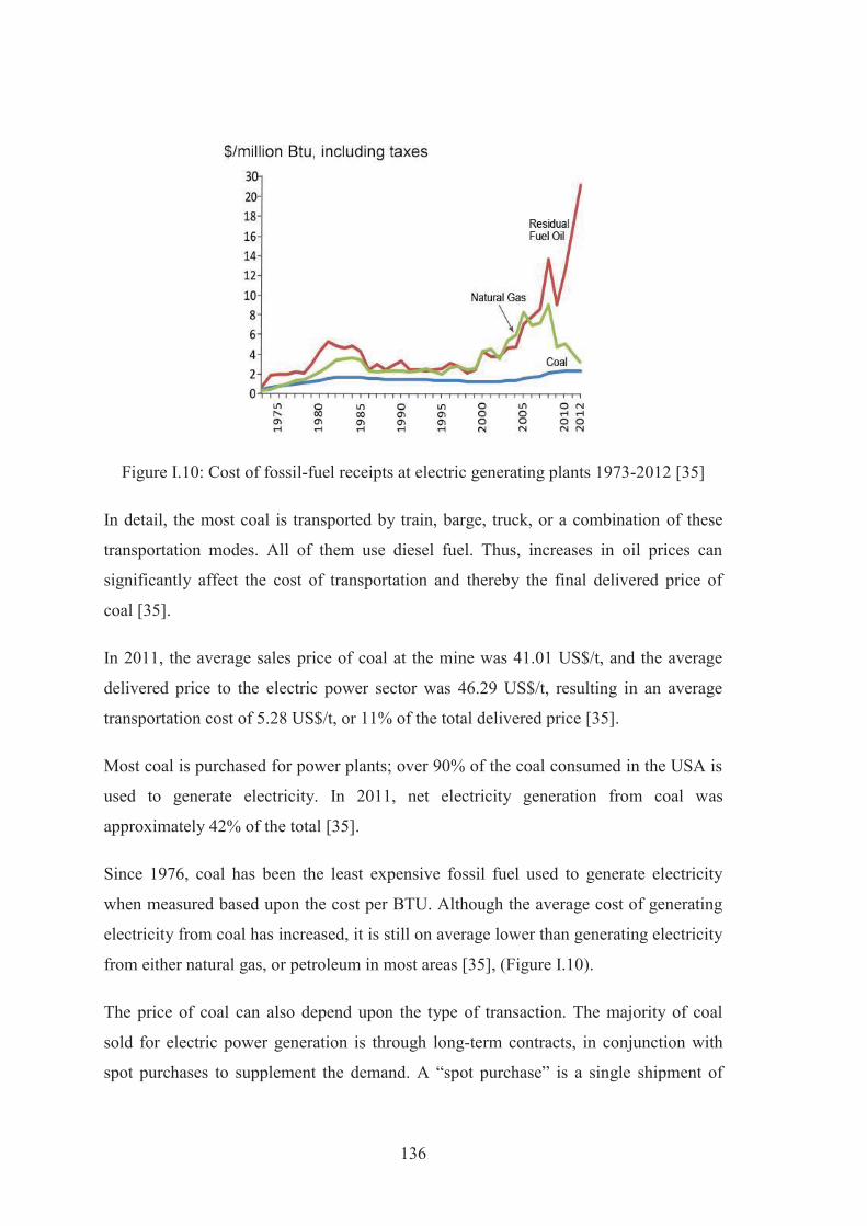
136
Figure I.10: Cost of fossil-fuel receipts at electric generating plants 1973-2012 [35]
In detail, the most coal is transported by train, barge, truck, or a combination of these
transportation modes. All of them use diesel fuel. Thus, increases in oil prices can
significantly affect the cost of transportation and thereby the final delivered price of
coal [35].
In 2011, the average sales price of coal at the mine was 41.01 US$/t, and the average
delivered price to the electric power sector was 46.29 US$/t, resulting in an average
transportation cost of 5.28 US$/t, or 11% of the total delivered price [35].
Most coal is purchased for power plants; over 90% of the coal consumed in the USA is
used to generate electricity. In 2011, net electricity generation from coal was
approximately 42% of the total [35].
Since 1976, coal has been the least expensive fossil fuel used to generate electricity
when measured based upon the cost per BTU. Although the average cost of generating
electricity from coal has increased, it is still on average lower than generating electricity
from either natural gas, or petroleum in most areas [35], (Figure I.10).
The price of coal can also depend upon the type of transaction. The majority of coal
sold for electric power generation is through long-term contracts, in conjunction with
spot purchases to supplement the demand. A “spot purchase” is a single shipment of
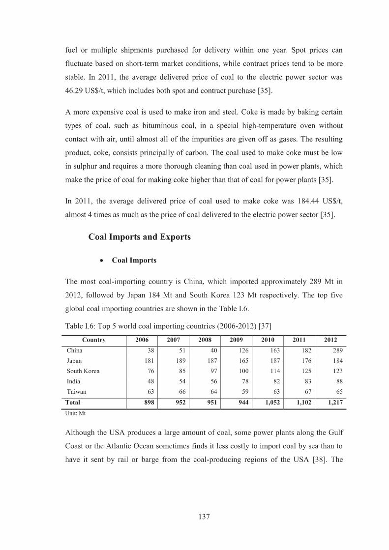
137
fuel or multiple shipments purchased for delivery within one year. Spot prices can
fluctuate based on short-term market conditions, while contract prices tend to be more
stable. In 2011, the average delivered price of coal to the electric power sector was
46.29 US$/t, which includes both spot and contract purchase [35].
A more expensive coal is used to make iron and steel. Coke is made by baking certain
types of coal, such as bituminous coal, in a special high-temperature oven without
contact with air, until almost all of the impurities are given off as gases. The resulting
product, coke, consists principally of carbon. The coal used to make coke must be low
in sulphur and requires a more thorough cleaning than coal used in power plants, which
make the price of coal for making coke higher than that of coal for power plants [35].
In 2011, the average delivered price of coal used to make coke was 184.44 US$/t,
almost 4 times as much as the price of coal delivered to the electric power sector [35].
Coal Imports and Exports
Coal Imports
The most coal-importing country is China, which imported approximately 289 Mt in
2012, followed by Japan 184 Mt and South Korea 123 Mt respectively. The top five
global coal importing countries are shown in the Table I.6.
Table I.6: Top 5 world coal importing countries (2006-2012) [37]
Country 2006 2007 2008 2009 2010 2011 2012 China 38 51 40 126 163 182 289 Japan 181 189 187 165 187 176 184 South Korea 76 85 97 100 114 125 123 India 48 54 56 78 82 83 88 Taiwan 63 66 64 59 63 67 65
Total 898 952 951 944 1,052 1,102 1,217 Unit: Mt
Although the USA produces a large amount of coal, some power plants along the Gulf
Coast or the Atlantic Ocean sometimes finds it less costly to import coal by sea than to
have it sent by rail or barge from the coal-producing regions of the USA [38]. The

138
history of coal export and import, and coal production and consumption in the USA are
shown in Figure I.11.
Figure I.11: Coal production, consumption, import, and export in USA. [38]
Of every billion tonnes of coal consumed in the USA in 2011, about 1% was imported,
mostly from South America. In 2011, the amount of coal imported into the USA was
about 12% of the amount exported to other countries [38].
Coal Exports
The first coal exporting country is Indonesia, which exported around 382 Mt in 2012,
followed by Australia with 301 Mt and Russia at 137 Mt respectively. The top five
world coal exporting countries are shown in Table I.7.
Table I.7: Top 5 world coal exporting countries (2006-2012) [39]
Country 2006 2007 2008 2009 2010 2011 2012 Indonesia 183 195 200 233 267 300 382 Australia 232 244 252 262 292 284 301 Russia 94 102 101 108 135 127 137 USA 46 55 46 55 75 98 115 Columbia 62 65 68 68 70 81 84
Total 926 962 968 947 1,098 1,166 1,282 Unit: Mt
The USA is a net exporter of coal, which means it exports more coal to other countries
than it imports. Between 2000 and 2010, about 5% of the coal produced in the USA, on

139
average, was exported to other countries. In 2011, the USA coal exports climbed to
10% (the highest level in two decades), partly because flooding disrupted coal mining in
Australia, which is normally the world's largest coal exporter. Coal exports come in two
forms: (1) metallurgical coal, which could be used for steel production, and (2) steam
coal, which can be used for electricity generation. Metallurgical coal dominated the
USA coal exports in 2011, with Europe the largest importer, followed by Asia [38].
Social and Environmental Problems of Coal Mining
There is much research focused on the social and environmental problems of mining
activities, some of which is specific in coal mining. The research presented in this
section, gives an overview of information for this thesis.
Slaby, (1992, 1998); Gerhardt and Slaby, (1994, 2000) referred to in Drebenstedt
(2006), and C. Roumpos et.al. (2004), [7, 40] said that “mining will always affect the
environment. Regions where raw materials are produced by surface mining are
particularly affected in this respect. The changes in nature caused by mining activities
are most varied. They include changes in agriculture and thus to the biosphere, the
temporary withdrawal of arable land and living space as well as their devastation, at
least for some time, infrastructural changes in the region and the interference in natural
and anthropogenic water systems. In order to secure the chances of future generations
for a sustainable development, the natural balance affected by mining activities will
therefore have to be redressed and the living space once given over to mining will have
to be revitalized”. Therefore, the mining companies have a responsibility to rehabilitate
to the area’s previous condition [6].
Bian, et al. (2010) studied the environmental issues from coal mining and their
solutions. This research showed that the environmental challenges of coal mining
include coal mine accidents, land subsidence, damage to the aquatic environment,
mining waste disposal, and air pollution. These are caused either by environmental
pollution or landscape change. A conceptual framework for solving mine environmental
issues was proposed. Clean processes, or remediation measures, are designed to address
environmental pollution [11], (Figure I.12).
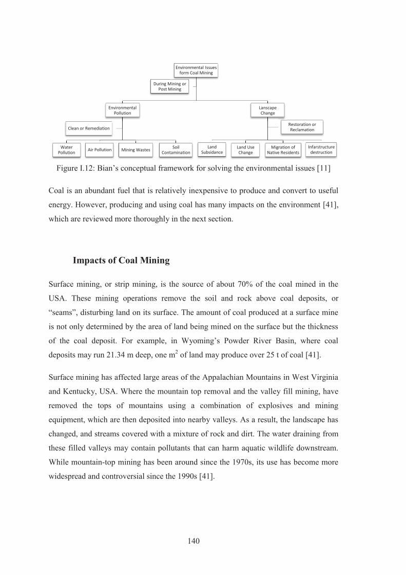
140
Figure I.12: Bian’s conceptual framework for solving the environmental issues [11]
Coal is an abundant fuel that is relatively inexpensive to produce and convert to useful
energy. However, producing and using coal has many impacts on the environment [41],
which are reviewed more thoroughly in the next section.
Impacts of Coal Mining
Surface mining, or strip mining, is the source of about 70% of the coal mined in the
USA. These mining operations remove the soil and rock above coal deposits, or
“seams”, disturbing land on its surface. The amount of coal produced at a surface mine
is not only determined by the area of land being mined on the surface but the thickness
of the coal deposit. For example, in Wyoming’s Powder River Basin, where coal
deposits may run 21.34 m deep, one m2 of land may produce over 25 t of coal [41].
Surface mining has affected large areas of the Appalachian Mountains in West Virginia
and Kentucky, USA. Where the mountain top removal and the valley fill mining, have
removed the tops of mountains using a combination of explosives and mining
equipment, which are then deposited into nearby valleys. As a result, the landscape has
changed, and streams covered with a mixture of rock and dirt. The water draining from
these filled valleys may contain pollutants that can harm aquatic wildlife downstream.
While mountain-top mining has been around since the 1970s, its use has become more
widespread and controversial since the 1990s [41].
Environmental Issues form Coal Mining
Environmental Pollution
Water Pollution
Air Pollution Mining Wastes Soil Contamination
Clean or Remediation
Lanscape Change
Land Subsidance
Land Use Change
Migration of Native Residents
Infarstructure destruction
Restoration or Reclamation
During Mining or Post Mining
141
The USA laws require that dust and water runoff from the affected area has to be
controlled, and the mining area has to be “reclaimed” close to its original condition.
Many surface mines have been reclaimed so well, that it can be hard to tell that there
was ever a surface mine in the area. However, there are areas that have not been
reclaimed as successfully [41].
While, underground mining has less overall impact on the environment than surface
mines. The most serious impact of underground mining may be the methane gas that
has to be vented out of mines to make them safe to work. Methane is a strong
greenhouse gas, meaning that on an equal-weight basis its global warming potential is
much higher than other greenhouse gases. In 2011, the most recent year for which
estimates are available, methane emissions from underground mines accounted for
about 7% of the USA total methane emissions, and 1% of the USA total greenhouse gas
emissions (based on global warming potential). Some mines capture and use, or sell, the
methane extracted from mines. Surface mines contribute about 2% of total methane
emissions [41]. However, the ground above mine tunnels can collapse, and acidic water
can drain from abandoned underground mines. Underground coal mining is a dangerous
profession, and coal miners can be injured or killed in mining accidents, especially in
countries without strict enforcement of safety regulations and procedures. Miners can
also get black lung disease from the coal dust in the mines [41].
Moreover, when coal is burned or ignited, harmful gases and others are produced. The
principal emissions resulting from coal combustion are [41]:
Sulphur dioxide (SO2), which contributes to acid rain and respiratory illnesses.
Nitrogen oxides (NOx), which contributes to smog and respiratory illnesses.
Particulates, which contribute to smog, haze, respiratory illnesses, and lung
disease.
Carbon dioxide (CO2), which is the primary greenhouse gas emission from the
burning of fossil fuels (coal, oil, and natural gas).
Mercury and other heavy metals, which have been linked with both
neurological and developmental damage in humans and other animals. Mercury
concentrations in the air usually are low and of little direct concern. However,
when mercury enters water – either directly or through deposition from the air –

142
biological processes transform it into methyl mercury, a highly toxic chemical
that accumulates in fish and the animals, including humans that eat fish.
Fly ash and bottom ash, are residuals created when coal is burned at power
plants. In the past, fly ash was released into the air through the smokestack, but
by modern regulations, fly ash must capture it with the pollution control devices,
like scrubbers. In the USA, fly ash is generally stored at coal power plants or
placed in landfills. Pollution leaching from ash storage and landfills into
groundwater and the rupture of several large impoundments of ash has emerged
as new environmental concerns.
However, through modern technology, industry has found several ways to reduce
sulphur dioxide (SO2), nitrogen oxides (NOx), and other impurities from coal. They
have found more effective ways of cleaning coal after it is mined, and coal consumers
have shifted towards greater use of low sulphur coal [41].
Power plants use the flue gas desulphurization equipment (FGD), also known as
“scrubbers”, to clean sulphur from the smoke before it leaves their smokestacks. In
addition, industries and governments have cooperated to develop technologies that can
remove impurities from coal or that make coal more energy-efficient, so less needs to
be burned [41].
The equipment intended mainly to reduce SO2, such as scrubbers, NOx, such as catalytic
converters, and particulate matter, such as electrostatic precipitators and bag houses, is
also able to reduce mercury emissions from some types of coal. At present, scientists
are also working on the new ways to reduce mercury emissions from coal-burning
power plants [41].
Furthermore, research is underway to address emissions of carbon dioxide from coal
combustion. Carbon capture separates CO2 from emissions sources and recovers it into
a concentrated stream. The CO2 can then be sequestered, which puts CO2 into storage,
possibly underground, in such a way that it will remain there permanently [41].
Finally, reuse and recycling can also reduce the environmental impact of coal. The area
that was previously used for coal mining can be reclaimed for uses like airports,
143
landfills, and golf courses, etc. Waste products captured by scrubbers can be used to
produce products like cement and synthetic gypsum for wallboard [41].
Mine Economic Valuation
Estimating Mining Cost
The cost of mining is one of the key factors that mining companies want to know and
analyse or estimate before deciding to invest in new mining projects [42]. The theory
and discussion of coal estimation are presented in the next section.
Types of Mining Costs
There are different types of costs, which are incurred in a mining operation. However,
Pfleider and Weaton (1968) proposed a way in which they can be reported in three
categories, which are [43, 44]:
Capital cost;
Operating cost;
General and administrative cost (G&A).
The capital cost might refer to the investment required for the mining and milling plant.
The operating costs would reflect drilling, blasting, loading, etc., costs incurred on a per
tonne basis. The G&A cost might be a yearly charge. It could include one or more of
the following: [43, 44]
Area supervision;
Mine supervision;
Employee benefits;
Overtime premium;
Mine office expense;
Head office expense;
Mine surveying;
Pumping;
Development drilling;
Payroll taxes;
State and local taxes;
Insurance;
Assaying;
Mine plant depreciation.
The capital and G&A costs could be translated into a cost per tonne basis like the
operating costs. Then the cost categories might become: [43, 44]
144
Ownership cost;
Production cost;
G&A cost.
The operating cost can be reported by the different unit operations: [43, 44]
Drilling;
Blasting;
Loading;
Hauling;
Others.
The “Others” category could be broken down to include dozing, grading, road
maintenance, dump maintenance, pumping, etc. Some mines include maintenance costs
together with the operating costs. Others might include it under G&A. Material cost
could be further detailed into components. For blasting this might mean: [43, 44]
Explosive;
Caps;
Primers;
Downlines.
The operating cost could just as easily be broken down for example into the categories:
[43, 44]
Labour;
Materials, Expenses, and Power (MEP);
Others.
At a given operation, the labour expense may include only the direct labour (driller, and
driller helper, for example). In another the indirect labour, such as supervision, repair,
etc., could be included as well [43, 44].
There are certain costs, which are regarded as “fixed”, or independent of the production
level. Other costs are “variable”, depending directly on production level. Other costs are
somewhere in between. Costs could be charged against the ore, against the waste, or
against both. For equipment, the ownership cost is often broken down into depreciation

145
and an average annual investment cost. The average annual investment cost may
include, for example taxes, insurance and interest rate. The bottom line is that when
discussing, calculating or presenting costs, one must be very careful to define what is
meant, and included, or not included. This section attempts to present a number of ways
in which costs of various types might be estimated [43, 44].
Mining Cost Estimation
This section discusses techniques for estimating mining costs, focusing on surface coal
mining costs. The mine operating cost estimation could start with a detailed unit cost of
ore and waste. It is presented in Table I.8.
Table I.8: Mining costs for ore and waste [43]
Activities (US$/t) Dozing and grading 0.05 Drilling 0.07 Blasting 0.13 Loading 0.14 Hauling 0.21 Crushing 0.11 Conveying 0.06 Pumping 0.01 Maintenance 0.10 Supervision 0.02 Other 0.02
Total 0.92
On the other hand, the whole mining cost estimation could be started with the analysis
of each part and period of the mining activities. It is discussed in the next section.
Mining Cost Estimation Technique
In 1980 O'Hara [43] published what has become a classic paper “Quick guides to the
evaluation of ore bodies”. They have since produced an updated version, which is used
in the textbook “Open Pit Mine Planning and Design” by W. A. Hustrulid and M.

146
Kuchta (1998, 2006). However, one of the original curves, which shows mine/mill
capital cost (C) to daily milling rate (Tp), will be used here to demonstrate cost
escalation procedures.
Generally, milling has a much larger capital cost per daily tonne of ore, and hence
dominates the curve. It is assumed that the mining operations run only 5 days a week,
but that the mill is operated continuously 7 days a week. Thus, the daily ore mined and
crushed (To) will be 40% higher than the milling rate (T): [43, 44]
where To = ore mining rate
T = milling rate
Daily Tonne of Material Mine
The most important factor affecting costs is the size of the mine, primary crusher, and a
processing plant, as expressed in terms of the tonnes of material handled per day of
operation. To simplify the discussion the following terms will be introduced: [43, 44]
T = tonnes of ore milled per day
To = tonnes of ore mined per day
Tw = tonnes of waste mined per day
Tc = tonnes of ore passing the primary crusher per day
Tp = To + Tw = total material mined per day
In this calculation, it is assumed that the mill operates three shifts per day and 7 days a
week regardless of the shifts worked by the open pit. Many open pit mines operate 7
days a week, but others may operate only 5 days a week. In the general case of 5 days a
week mining operation [43, 44]. The relationship is shown in equation (I.2).
The cost guides in this calculation process are based upon the assumption that the mill
capacity is 71% of the daily mined ore. The crushing plant may operate 5, 6, or 7 days a
week, depending on the mine schedule and whether or not there is adequate fine ore
(I.1)
(I.2)
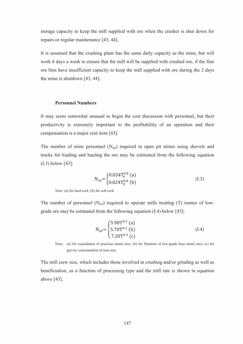
147
storage capacity to keep the mill supplied with ore when the crusher is shut down for
repairs or regular maintenance [43, 44].
It is assumed that the crushing plant has the same daily capacity as the mine, but will
work 6 days a week to ensure that the mill will be supplied with crushed ore, if the fine
ore bins have insufficient capacity to keep the mill supplied with ore during the 2 days
the mine is shutdown [43, 44].
Personnel Numbers
It may seem somewhat unusual to begin the cost discussion with personnel, but their
productivity is extremely important to the profitability of an operation and their
compensation is a major cost item [43].
The number of mine personnel (Nop) required in open pit mines using shovels and
trucks for loading and hauling the ore may be estimated from the following equation
(I.3) below [43]:
Note: (a) for hard rock; (b) for soft rock.
The number of personnel (Nml) required to operate mills treating (T) tonnes of low-
grade ore may be estimated from the following equation (I.4) below [43]:
Note: (a) for cyanidation of precious metal ores; (b) for flotation of low-grade base metal ores; (c) for
gravity concentration of iron ores.
The mill crew size, which includes those involved in crushing and/or grinding as well as
beneficiation, as a function of processing type and the mill rate is shown in equation
above [43].
(I.3)
(I.4)
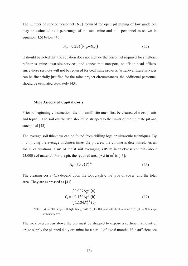
148
The number of service personnel (Nsv) required for open pit mining of low grade ore
may be estimated as a percentage of the total mine and mill personnel as shown in
equation (I.5) below [43]:
It should be noted that the equation does not include the personnel required for smelters,
refineries, mine town-site services, and concentrate transport, or offsite head offices,
since these services will not be required for coal mine projects. Whenever these services
can be financially justified for the mine project circumstances, the additional personnel
should be estimated separately [43].
Mine Associated Capital Costs
Prior to beginning construction, the mine/mill site must first be cleared of trees, plants
and topsoil. The soil overburden should be stripped to the limits of the ultimate pit and
stockpiled [43].
The average soil thickness can be found from drilling logs or ultrasonic techniques. By
multiplying the average thickness times the pit area, the volume is determined. As an
aid in calculations, a m2 of moist soil averaging 3.05 m in thickness contains about
23,000 t of material. For the pit, the required area (Ap) in m2 is [43]:
The clearing costs (Cc) depend upon the topography, the type of cover, and the total
area. They are expressed as [43]:
Note: (a) for 20% slope with light tree growth; (b) for flat land with shrubs and no tree; (c) for 30% slope
with heavy tree
The rock overburden above the ore must be stripped to expose a sufficient amount of
ore to supply the planned daily ore mine for a period of 4 to 6 months. If insufficient ore
(I.5)
(I.6)
(I.7)
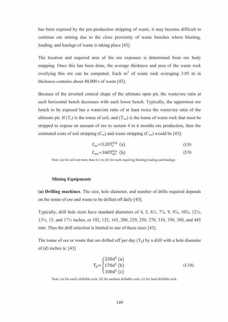
149
has been exposed by the pre-production stripping of waste, it may become difficult to
continue ore mining due to the close proximity of waste benches where blasting,
loading, and haulage of waste is taking place [43].
The location and required area of the ore exposure is determined from ore body
mapping. Once this has been done, the average thickness and area of the waste rock
overlying this ore can be computed. Each m2 of waste rock averaging 3.05 m in
thickness contains about 40,000 t of waste [43].
Because of the inverted conical shape of the ultimate open pit, the waste/ore ratio at
each horizontal bench decreases with each lower bench. Typically, the uppermost ore
bench to be exposed has a waste/ore ratio of at least twice the waste/ore ratio of the
ultimate pit. If (Ts) is the tonne of soil, and (Tws) is the tonne of waste rock that must be
stripped to expose an amount of ore to sustain 4 to 6 months ore production, then the
estimated costs of soil stripping (Css) and waste stripping (Cws) would be [43]:
Note: (a) for soil not more than 6.1 m; (b) for rock requiring blasting loading and haulage.
Mining Equipments
(a) Drilling machines. The size, hole diameter, and number of drills required depends
on the tonne of ore and waste to be drilled off daily [43].
Typically, drill hole sizes have standard diameters of 4, 5, 6½, 7⅞, 9, 9⅞, 10⅝, 12¼,
13¾, 15, and 17½ inches, or 102, 125, 165, 200, 229, 250, 270, 310, 350, 380, and 445
mm. Thus the drill selection is limited to one of these sizes [43].
The tonne of ore or waste that are drilled off per day (Td) by a drill with a hole diameter
of (d) inches is: [43]
Note: (a) for easily drillable rock; (b) for medium drillable rock; (c) for hard drillable rock.
(I.8)
(I.9)
(I.10)
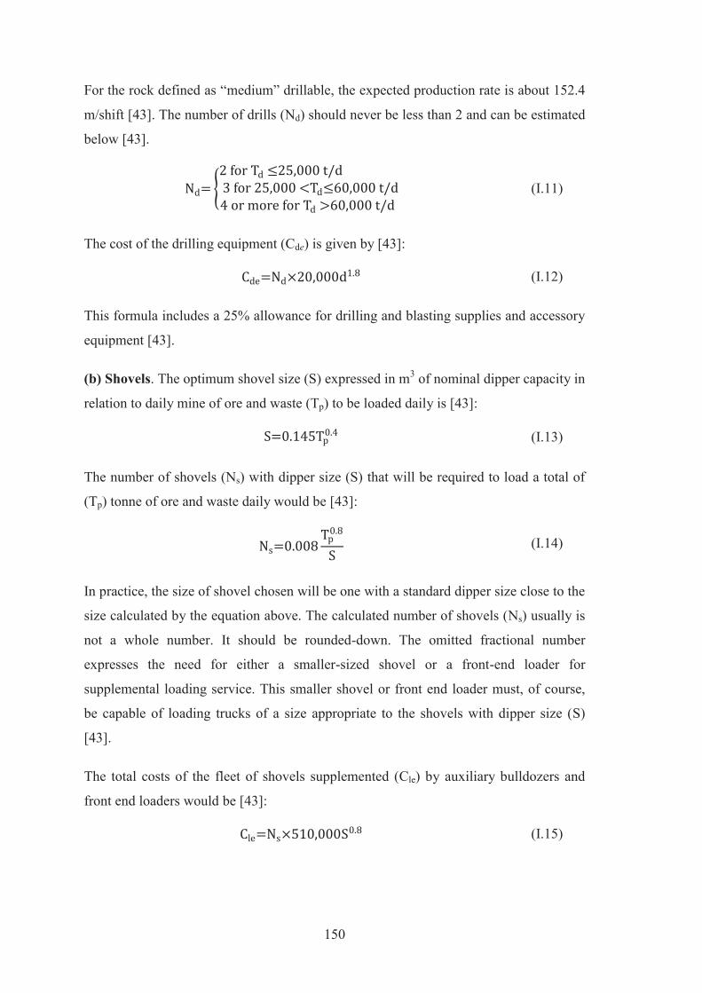
150
For the rock defined as “medium” drillable, the expected production rate is about 152.4
m/shift [43]. The number of drills (Nd) should never be less than 2 and can be estimated
below [43].
The cost of the drilling equipment (Cde) is given by [43]:
This formula includes a 25% allowance for drilling and blasting supplies and accessory
equipment [43].
(b) Shovels. The optimum shovel size (S) expressed in m3 of nominal dipper capacity in
relation to daily mine of ore and waste (Tp) to be loaded daily is [43]:
The number of shovels (Ns) with dipper size (S) that will be required to load a total of
(Tp) tonne of ore and waste daily would be [43]:
In practice, the size of shovel chosen will be one with a standard dipper size close to the
size calculated by the equation above. The calculated number of shovels (Ns) usually is
not a whole number. It should be rounded-down. The omitted fractional number
expresses the need for either a smaller-sized shovel or a front-end loader for
supplemental loading service. This smaller shovel or front end loader must, of course,
be capable of loading trucks of a size appropriate to the shovels with dipper size (S)
[43].
The total costs of the fleet of shovels supplemented (Cle) by auxiliary bulldozers and
front end loaders would be [43]:
(I.11)
(I.12)
(I.13)
(I.14)
(I.15)
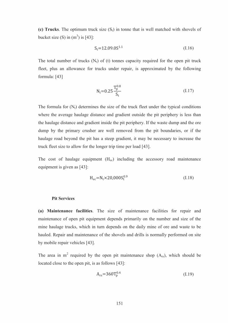
151
(c) Trucks. The optimum truck size (St) in tonne that is well matched with shovels of
bucket size (S) in (m3) is [43]:
The total number of trucks (Nt) of (t) tonnes capacity required for the open pit truck
fleet, plus an allowance for trucks under repair, is approximated by the following
formula: [43]
The formula for (Nt) determines the size of the truck fleet under the typical conditions
where the average haulage distance and gradient outside the pit periphery is less than
the haulage distance and gradient inside the pit periphery. If the waste dump and the ore
dump by the primary crusher are well removed from the pit boundaries, or if the
haulage road beyond the pit has a steep gradient, it may be necessary to increase the
truck fleet size to allow for the longer trip time per load [43].
The cost of haulage equipment (Hec) including the accessory road maintenance
equipment is given as [43]:
Pit Services
(a) Maintenance facilities. The size of maintenance facilities for repair and
maintenance of open pit equipment depends primarily on the number and size of the
mine haulage trucks, which in turn depends on the daily mine of ore and waste to be
hauled. Repair and maintenance of the shovels and drills is normally performed on site
by mobile repair vehicles [43].
The area in m2 required by the open pit maintenance shop (Ars), which should be
located close to the open pit, is as follows [43]:
(I.16)
(I.17)
(I.18)
(I.19)
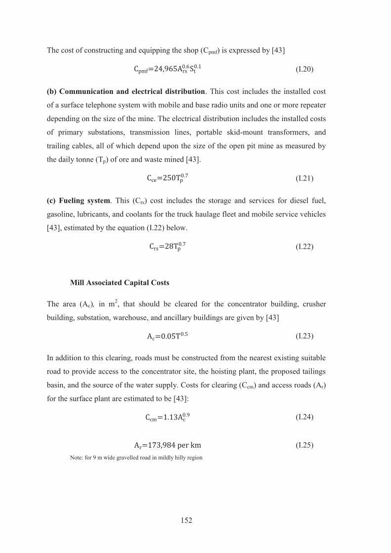
152
The cost of constructing and equipping the shop (Cpmf) is expressed by [43]
(b) Communication and electrical distribution. This cost includes the installed cost
of a surface telephone system with mobile and base radio units and one or more repeater
depending on the size of the mine. The electrical distribution includes the installed costs
of primary substations, transmission lines, portable skid-mount transformers, and
trailing cables, all of which depend upon the size of the open pit mine as measured by
the daily tonne (Tp) of ore and waste mined [43].
(c) Fueling system. This (Crs) cost includes the storage and services for diesel fuel,
gasoline, lubricants, and coolants for the truck haulage fleet and mobile service vehicles
[43], estimated by the equation (I.22) below.
Mill Associated Capital Costs
The area (Ac), in m2, that should be cleared for the concentrator building, crusher
building, substation, warehouse, and ancillary buildings are given by [43]
In addition to this clearing, roads must be constructed from the nearest existing suitable
road to provide access to the concentrator site, the hoisting plant, the proposed tailings
basin, and the source of the water supply. Costs for clearing (Ccm) and access roads (Ar)
for the surface plant are estimated to be [43]:
Note: for 9 m wide gravelled road in mildly hilly region
(I.20)
(I.21)
(I.22)
(I.23)
(I.24)
(I.25)
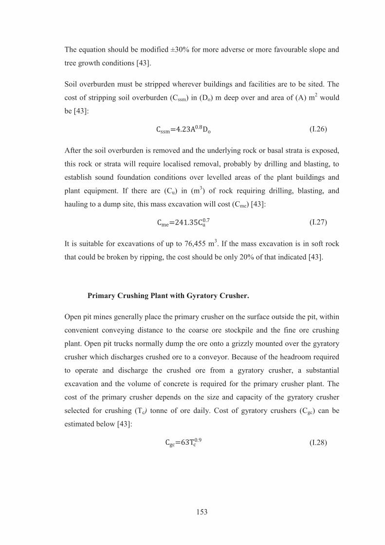
153
The equation should be modified ±30% for more adverse or more favourable slope and
tree growth conditions [43].
Soil overburden must be stripped wherever buildings and facilities are to be sited. The
cost of stripping soil overburden (Cssm) in (Do) m deep over and area of (A) m2 would
be [43]:
After the soil overburden is removed and the underlying rock or basal strata is exposed,
this rock or strata will require localised removal, probably by drilling and blasting, to
establish sound foundation conditions over levelled areas of the plant buildings and
plant equipment. If there are (Cu) in (m3) of rock requiring drilling, blasting, and
hauling to a dump site, this mass excavation will cost (Cme) [43]:
It is suitable for excavations of up to 76,455 m3. If the mass excavation is in soft rock
that could be broken by ripping, the cost should be only 20% of that indicated [43].
Primary Crushing Plant with Gyratory Crusher.
Open pit mines generally place the primary crusher on the surface outside the pit, within
convenient conveying distance to the coarse ore stockpile and the fine ore crushing
plant. Open pit trucks normally dump the ore onto a grizzly mounted over the gyratory
crusher which discharges crushed ore to a conveyor. Because of the headroom required
to operate and discharge the crushed ore from a gyratory crusher, a substantial
excavation and the volume of concrete is required for the primary crusher plant. The
cost of the primary crusher depends on the size and capacity of the gyratory crusher
selected for crushing (Tc) tonne of ore daily. Cost of gyratory crushers (Cgc) can be
estimated below [43]:
(I.26)
(I.27)
(I.28)

154
The cost of primary crusher plant (Cpcp), installing the crusher, construction of the truck
dump and grizzly, plus the coarse ore conveyor and feeder under the crusher is [43]:
General Plant Services.
These costs include the costs of constructing, furnishing, and equipping the general
administrative office, general warehouse, electrical and mechanical repair shop for
smaller mill equipment and service equipment, vehicle garages, change houses, first aid
and mine rescue stations, security stations plus general purpose vehicles, parking lots,
and yard fencing [43].
The size of the buildings tends to depend upon the number of employees served by each
building. It is necessary to estimate the building size in m2 before estimating building
cost, which will vary with the area of each type of building [43].
(a) Administrative office. The floor space per person tends to increase as the number
of administrative and technical staff (Nat) becomes larger. This reflects the more
complex records of accounting and technical staff and the consequent requirement of
more space for computer facilities, mining plans, and reference file facilities. The
administrative office area (Aof) required in (m2) can be estimated with the formula
below [43, 44].
The cost of office buildings (Cof) can be estimated with the equation (I.31) [43, 44].
(b) Maintenance shop. Maintenance personnel (Nsv) will require approximately 8.0
m2/person for maintenance and repair of movable equipment of the mill and service
departments. Cost of maintenance shop (Csh) should be estimated by equation (I.32)
below [43, 44].
(I.29)
(I.30)
(I.31)

155
(c) Mine changehouse. The mine changehouse requires about 2.23 m2 per person on
the mine payroll and includes the first aid station and mine rescue facilities. Cost of
mine changehouse (Chc) shown below [43, 44].
(d) Surface warehouse. This should accommodate all supplies and spare parts for the
mine, mill, and service facilities that must be kept indoors. Bulky supplies such as
rough lumber, structural steel, etc., can be stored outdoors in most climates. The surface
warehouse cost (Csw) can be estimated by equation (I.34) below [43, 44].
(e) Miscellaneous surface facilities. It includes general purpose vehicles and garages,
security stations and fencing, parking lots, and miscellaneous services. The
miscellaneous surface facilities cost (Cmsf) could be estimated by equation (I.35) below
[43, 44].
Mine Project Overhead Costs
In addition to the direct costs for specific facilities for a mine project, which may total
many millions US$, there are substantial costs and expenses involved in project design,
general site costs, supervision and administration, and provision of working capital.
These overhead costs could be estimated as a function of the total direct costs (D) in
US$ [43, 44].
(a) Engineering costs. This includes the costs of feasibility studies, environmental
impact studies, engineering design, equipment specifications and procurement, and
specialised consulting services. Engineering costs (Ec) can be estimated by equation
(I.36) below [43, 44].
(I.32)
(I.33)
(I.34)
(I.35)
(I.36)
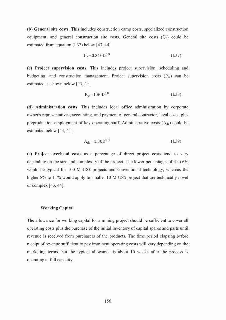
156
(b) General site costs. This includes construction camp costs, specialized construction
equipment, and general construction site costs. General site costs (Gc) could be
estimated from equation (I.37) below [43, 44].
(c) Project supervision costs. This includes project supervision, scheduling and
budgeting, and construction management. Project supervision costs (Psc) can be
estimated as shown below [43, 44].
(d) Administration costs. This includes local office administration by corporate
owner's representatives, accounting, and payment of general contractor, legal costs, plus
preproduction employment of key operating staff. Administrative costs (Adc) could be
estimated below [43, 44].
(e) Project overhead costs as a percentage of direct project costs tend to vary
depending on the size and complexity of the project. The lower percentages of 4 to 6%
would be typical for 100 M US$ projects and conventional technology, whereas the
higher 8% to 11% would apply to smaller 10 M US$ project that are technically novel
or complex [43, 44].
Working Capital
The allowance for working capital for a mining project should be sufficient to cover all
operating costs plus the purchase of the initial inventory of capital spares and parts until
revenue is received from purchasers of the products. The time period elapsing before
receipt of revenue sufficient to pay imminent operating costs will vary depending on the
marketing terms, but the typical allowance is about 10 weeks after the process is
operating at full capacity.
(I.37)
(I.38)
(I.39)
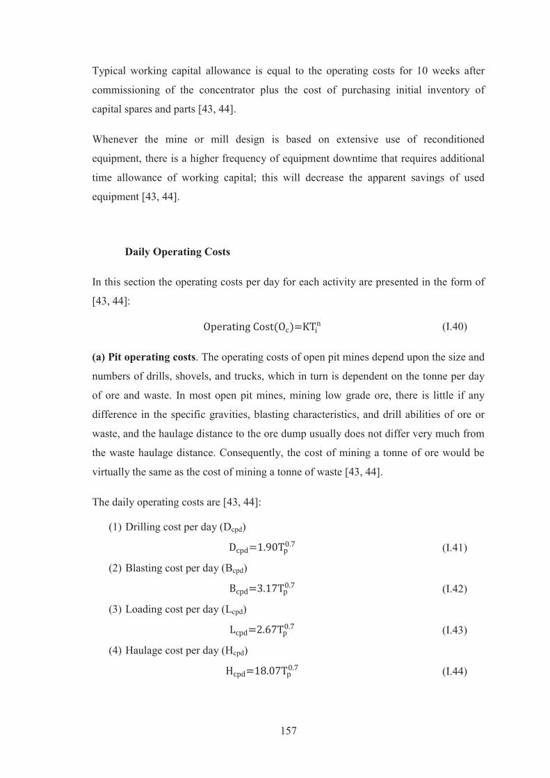
157
Typical working capital allowance is equal to the operating costs for 10 weeks after
commissioning of the concentrator plus the cost of purchasing initial inventory of
capital spares and parts [43, 44].
Whenever the mine or mill design is based on extensive use of reconditioned
equipment, there is a higher frequency of equipment downtime that requires additional
time allowance of working capital; this will decrease the apparent savings of used
equipment [43, 44].
Daily Operating Costs
In this section the operating costs per day for each activity are presented in the form of
[43, 44]:
(a) Pit operating costs. The operating costs of open pit mines depend upon the size and
numbers of drills, shovels, and trucks, which in turn is dependent on the tonne per day
of ore and waste. In most open pit mines, mining low grade ore, there is little if any
difference in the specific gravities, blasting characteristics, and drill abilities of ore or
waste, and the haulage distance to the ore dump usually does not differ very much from
the waste haulage distance. Consequently, the cost of mining a tonne of ore would be
virtually the same as the cost of mining a tonne of waste [43, 44].
The daily operating costs are [43, 44]:
(1) Drilling cost per day (Dcpd)
(2) Blasting cost per day (Bcpd)
(3) Loading cost per day (Lcpd)
(4) Haulage cost per day (Hcpd)
(I.40)
(I.41)
(I.42)
(I.43)
(I.44)
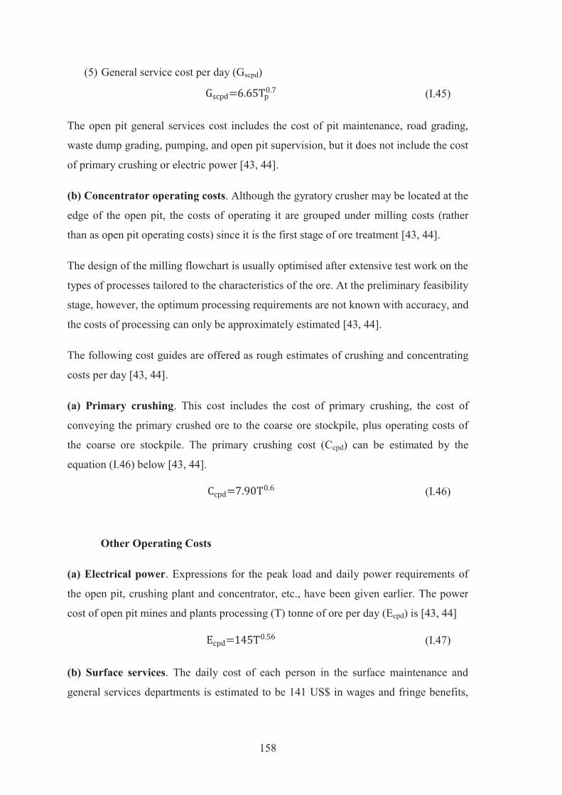
158
(5) General service cost per day (Gscpd)
The open pit general services cost includes the cost of pit maintenance, road grading,
waste dump grading, pumping, and open pit supervision, but it does not include the cost
of primary crushing or electric power [43, 44].
(b) Concentrator operating costs. Although the gyratory crusher may be located at the
edge of the open pit, the costs of operating it are grouped under milling costs (rather
than as open pit operating costs) since it is the first stage of ore treatment [43, 44].
The design of the milling flowchart is usually optimised after extensive test work on the
types of processes tailored to the characteristics of the ore. At the preliminary feasibility
stage, however, the optimum processing requirements are not known with accuracy, and
the costs of processing can only be approximately estimated [43, 44].
The following cost guides are offered as rough estimates of crushing and concentrating
costs per day [43, 44].
(a) Primary crushing. This cost includes the cost of primary crushing, the cost of
conveying the primary crushed ore to the coarse ore stockpile, plus operating costs of
the coarse ore stockpile. The primary crushing cost (Ccpd) can be estimated by the
equation (I.46) below [43, 44].
Other Operating Costs
(a) Electrical power. Expressions for the peak load and daily power requirements of
the open pit, crushing plant and concentrator, etc., have been given earlier. The power
cost of open pit mines and plants processing (T) tonne of ore per day (Ecpd) is [43, 44]
(b) Surface services. The daily cost of each person in the surface maintenance and
general services departments is estimated to be 141 US$ in wages and fringe benefits,
(I.45)
(I.46)
(I.47)

159
and an average cost of 16 US$ in supplies consumed. If the number of maintenance and
general services personnel is (Nsv), then the daily costs of maintenance and general
services departments (Scpd) is [43, 44]
The daily costs of the administrative and technical staff (Acpd), including supplies and
services required by them, and fixed costs for local property taxes and legal fees paid by
administrative services, are proportional to the number of staff (Nat). Each staff person
is estimated to cost on the average 185 US$ in salary per day, and to consume 37.60
US$ in supplies and services per day [43, 44].
Society Environment and Mine Closure Cost
There are some research and information related to society, environment and mine
closure. Some of this information is used to generate an overview of the ideas in this
thesis and to provide some data for the model development and simulation scenarios.
A. H. Watson (2006) tried to estimate mine closure cost with more accuracy [45] by
using risk management techniques. This explained a way to estimate mine closure cost
accurately, by using the probabilistic analysis, which was supported by Monte-Carlo
simulation and detail variables analysis.
Drebenstedt (2006) [40] presented the methodology of financial valuation of mine
closure alternatives. The mathematical valuation model is shown in equation (I.50):
Where AW = expense parameter,
At (0) = periodic amount of the cash-layout costs and investments in period t
at the valuation level in the base year (0),
q = imputed interest (the real rate of interest) [40].
(I.48)
(I.49)
(I.50)

160
L. Wilde (2007) [46], analysed the cost of mine closure from many countries around the
world. The factors affecting closure costs fall into two categories; (1) aspects of mining
such as, the mining method, the nature of the ore/mineral, the age of the mine, the
degree of on-site processing and wastes generated and (2) the context in which these
occur. The context is effectively, or at least can be, a “weighting” on costs that increases
the need for particular closure activities and stakeholder requirements because of
sensitivity.
A. Peralta-Romero and K. Dagdelen (2007) [47] developed a new model for estimation
of mine closure costs. The closure activities here were divided into 4 parts, (1)
exploration, (2) mine and process, (3) facilities, and (4) global activities. All closure
activities affect the general reclamation and closure procedures, including; (1)
earthwork, (2) revegetation, (3) drainage, and (4) water treatment. By using Excel with
Visual Basic for Applications (VBA), the model of mine closure cost estimation was
created.
I. M. Weiersbye (2007) [48] reviewed the cost of mine closure, and comparative cost of
conventional and phytotechnologies for mine closure. He summarised that the
estimation of cleanup costs for mine closure is complicated by the presence of
contaminants in waste, soil, and groundwater. Therefore, an area requires combinations
or successions of treatments for rehabilitation. The cost of non-biological technologies
for soils ranges from 10 to 4,000 US$/m3, and from 0.1 to 3.0 M US$/ha. For
groundwater this varies from lower than 1 to 300 US$/m3, but with phytotechnology
costs range from 0.02 to 10 US$/m3, or 200 to 100,000 US$/ha, and 0.2 to 40 US$/m3
of water.
Economic Decision Criteria
The general decisions on investment in business mainly rely upon economic decisions,
especially in mining companies. In this section, reviews of the theory of economic
decisions and research related to the evaluation of mining project are put forward.
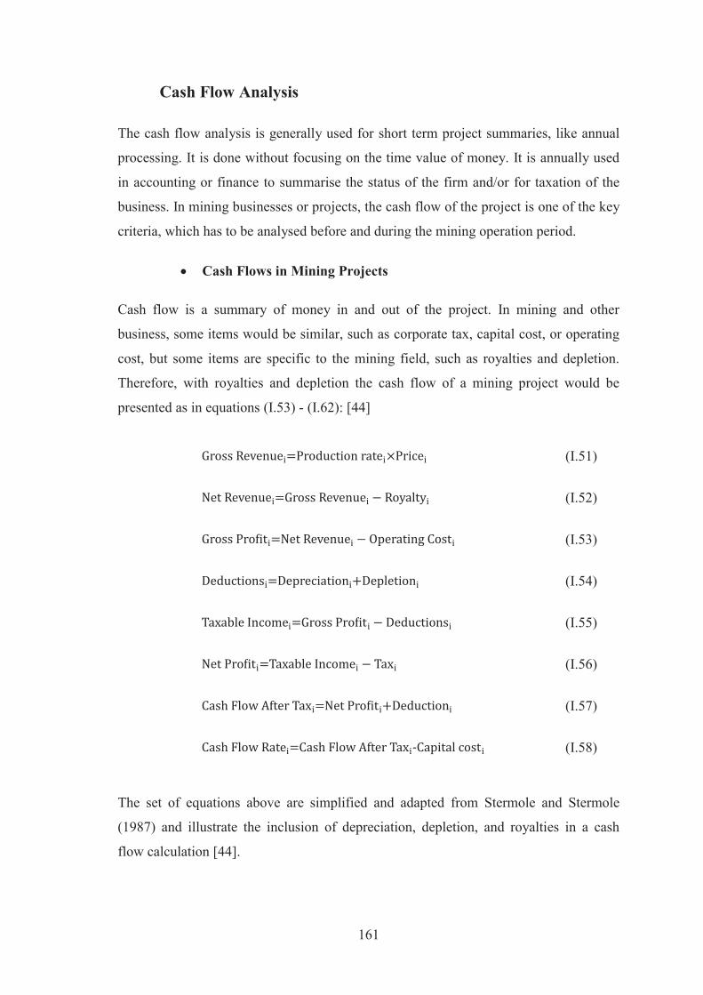
161
Cash Flow Analysis
The cash flow analysis is generally used for short term project summaries, like annual
processing. It is done without focusing on the time value of money. It is annually used
in accounting or finance to summarise the status of the firm and/or for taxation of the
business. In mining businesses or projects, the cash flow of the project is one of the key
criteria, which has to be analysed before and during the mining operation period.
Cash Flows in Mining Projects
Cash flow is a summary of money in and out of the project. In mining and other
business, some items would be similar, such as corporate tax, capital cost, or operating
cost, but some items are specific to the mining field, such as royalties and depletion.
Therefore, with royalties and depletion the cash flow of a mining project would be
presented as in equations (I.53) - (I.62): [44]
The set of equations above are simplified and adapted from Stermole and Stermole
(1987) and illustrate the inclusion of depreciation, depletion, and royalties in a cash
flow calculation [44].
(I.51)
(I.52)
(I.53)
(I.54)
(I.55)
(I.56)
(I.57)
(I.58)

162
Discount Cash Flow Analysis
The Decision Making on Investment Theory
The analysis of Discounted Cash Flow (DCF) is a way to decide on investment in
general and mining businesses. As the value of money changes all the time, money
tomorrow is not as valuable as money today, so money in the future needs to be
calculated to a value relating to the present for comparison. The equations of PV and
NPV are shown below [9, 49].
The Present Value (PV) and Net Present Value (NPV)
(a) PV equation [9]:
where
t = the time of the cash flow,
i = the discount rate (the rate of return that could be earned on an investment in the financial markets with similar risk.),
Rt = the Net Cash Flow (the amount of cash: inflow - outflow) at time t. For educational purposes, R0 is commonly placed to the left of the sum to emphasise its role as (minus) the investment. Sometime, the name, future value (FV) is used.
(b) NPV equation [9]:
NPV is an indicator of how much value an investment or project adds to the firm. With
a particular project, if Rt is a positive value, the project is in the status of discounted
cash inflow in the time (t). If Rt is a negative value, the project is in the status of
discounted cash outflow at the time (t). Appropriately, risked projects with a positive
NPV could be accepted. This does not necessarily mean that they should be undertaken
(I.59)
(I.60)
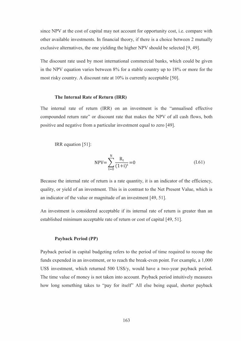
163
since NPV at the cost of capital may not account for opportunity cost, i.e. compare with
other available investments. In financial theory, if there is a choice between 2 mutually
exclusive alternatives, the one yielding the higher NPV should be selected [9, 49].
The discount rate used by most international commercial banks, which could be given
in the NPV equation varies between 8% for a stable country up to 18% or more for the
most risky country. A discount rate at 10% is currently acceptable [50].
The Internal Rate of Return (IRR)
The internal rate of return (IRR) on an investment is the “annualised effective
compounded return rate” or discount rate that makes the NPV of all cash flows, both
positive and negative from a particular investment equal to zero [49].
IRR equation [51]:
Because the internal rate of return is a rate quantity, it is an indicator of the efficiency,
quality, or yield of an investment. This is in contrast to the Net Present Value, which is
an indicator of the value or magnitude of an investment [49, 51].
An investment is considered acceptable if its internal rate of return is greater than an
established minimum acceptable rate of return or cost of capital [49, 51].
Payback Period (PP)
Payback period in capital budgeting refers to the period of time required to recoup the
funds expended in an investment, or to reach the break-even point. For example, a 1,000
US$ investment, which returned 500 US$/y, would have a two-year payback period.
The time value of money is not taken into account. Payback period intuitively measures
how long something takes to “pay for itself” All else being equal, shorter payback
(I.61)

164
periods are preferable to longer payback periods. The payback period is popular due to
its ease of use despite the recognised limitations described below [10].
The term is also widely used in other types of investment areas, often with respect to
energy efficiency technologies, maintenance, upgrades, or other changes. For example,
a compact fluorescent light bulb may be described as having a payback period of a
certain number of years or operating hours, assuming certain costs. Here, the return of
the investment consists of reduced operating costs. Although primarily a financial term,
the concept of a payback period is occasionally extended to other uses, such as the
energy payback period (the period of time over which the energy savings of a project
equal the amount of energy expended since project inception); these other terms may
not be standardised or widely used [10].
PP equation:
Payback period as a tool of analysis is often used because it is easy to apply and easy to
understand for most individuals, regardless of academic training or field of endeavour.
When used carefully or to compare similar investments, it can be quite useful. As a
stand-alone tool to compare an investment to “doing nothing” payback period has no
explicit criteria for decision-making (except, perhaps, that the payback period should be
less than infinity) [10].
The payback period is considered a method of analysis with serious limitations and
qualifications for its use, because it does not account for the time value of money, risk,
financing, or other important considerations, such as the opportunity cost. Whilst the
time value of money could be rectified, by applying a weighted average cost of capital
discount, it is generally agreed that this tool for investment decisions should not be used
in isolation. Alternative measures of “return” preferred by economists are Net Present
Value and internal rate of return. An implicit assumption in the use of payback period is
that returns to the investment continue after the payback period. Payback period does
not specify any required comparison to other investments or even to not making an
investment [10].
(I.62)
165
Mining Project Evaluation
There is much research focusing on mine economics, management, and financial
analysis of mining projects. This section reviews some interesting research, the ideas
and information of which can be used to continue in this thesis.
The computer is a useful tool, which has been used to evaluate mining projects for a
long time. In 2004, J. Cech, et.al., proposed a computerised evaluation of mining
projects by using spreadsheets and developing a user interface for easier use. The five
important keys design of the model were, (1) reserves flow and balance over time, (2)
cash flow statement and balance sheet over time, (3) investment and financial analysis
over time, (4) sensibility and risk analysis, and (5) what-if and scenario analysis. The
model was tested on some mining in the Czech Republic and Slovakia [52].
C. Drebenstedt, et.al. (2004) [53], (2006) [40], and (2010) [54] continued to evaluate
the activities of the post-mining period or mine closure period. This research proved the
new important trend of mine closure period, must be included in mining project
decisions and that finances of this period must be considered in the cash flow of the
mining project.
M. Osanloo, et.al. (2004) [54] developed an application software for open pit mining
cost estimation, which used O’Hara’s detail of cost estimation equations. The
application software was written in Visual Basic. The comparison technique of cost
estimation shows the cost estimate in this detailed technique is a better result than
O’Hara’ s technique, but with respect to the facility, speed, and the input-output
parameter ratio, O’Hara’s technique is superior. Moreover, the research suggested using
O’Hara’s technique for estimating the cost in the initial stage of the mining project, and
then when the project has more data or information, the detail technique of cost
estimates could be used in the final stage.

166
II. APPENDIX 2: ADDITIONAL INFORMATION TABLE
Table II.1: The lignite production of Thailand (1987-2012) [66, 67]
Year Lignite (t) EGAT Others Total
Mae Moh Krabi Total 1987 5,564,537 191,000 5,755,537 1,175,721 6,931,257 1988 5,717,250 237,396 5,954,646 1,340,413 7,295,059 1989 6,541,191 318,585 6,859,776 2,150,146 9,009,922 1990 9,652,991 156,262 9,809,254 2,629,219 12,438,473 1991 11,513,775 242,699 11,756,475 2,889,540 14,646,015 1992 11,844,352 253,950 12,098,302 3,290,259 15,388,561 1993 11,221,088 211,800 11,432,888 4,105,039 15,537,927 1994 11,906,553 225,065 12,131,618 4,963,253 17,094,871 1995 13,191,880 144,232 13,336,112 5,084,686 18,420,798 1996 16,381,301 16,381,301 5,309,093 21,690,394 1997 17,692,415 17,692,415 5,746,141 23,438,556 1998 14,419,327 14,419,327 5,576,868 19,996,195 1999 12,021,265 12,021,265 6,240,043 18,261,308 2000 13,621,615 30,000 13,651,615 4,134,132 17,785,747 2001 15,314,436 133,000 15,447,436 4,159,559 19,606,995 2002 14,994,739 187,000 15,181,739 4,420,245 19,601,984 2003 15,591,841 146,000 15,737,841 3,105,554 18,843,395 2004 16,561,572 95,868 16,657,440 3,402,404 20,059,844 2005 16,534,142 36,522 16,570,664 4,307,512 20,878,176 2006 15,763,798 56,000 15,819,798 3,250,810 19,070,608 2007 16,117,809 27,112 16,144,921 2,094,255 18,239,176 2008 16,420,847 23,248 16,444,095 1,651,290 18,095,385 2009 15,631,766 15,631,766 1,934,334 17,566,100 2010 15,987,263 15,987,263 2,270,799 18,258,062 2011 17,558,336 17,558,336 3,768,770 21,327,106 2012 16,590,461 16,590,461 1,475,968 18,066,429
Sum. 354,356,550 2,715,739 357,072,291 90,476,053 447,548,343 Max. 17,692,415 318,585 17,692,415 6,240,043 23,438,556 Min. 5,564,537 23,248 5,755,537 1,175,721 6,931,257 Ave. 13,629,098 150,874 13,733,550 3,479,848 17,213,398 S.D. 3,552,548 90,273 3,476,428 1,473,750 4,176,739
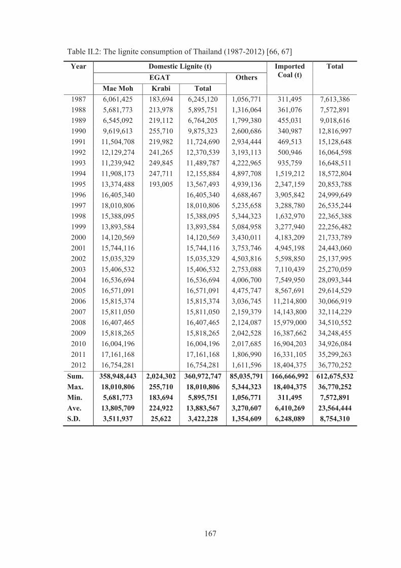
167
Table II.2: The lignite consumption of Thailand (1987-2012) [66, 67]
Year Domestic Lignite (t) Imported Coal (t)
Total EGAT Others
Mae Moh Krabi Total 1987 6,061,425 183,694 6,245,120 1,056,771 311,495 7,613,386 1988 5,681,773 213,978 5,895,751 1,316,064 361,076 7,572,891 1989 6,545,092 219,112 6,764,205 1,799,380 455,031 9,018,616 1990 9,619,613 255,710 9,875,323 2,600,686 340,987 12,816,997 1991 11,504,708 219,982 11,724,690 2,934,444 469,513 15,128,648 1992 12,129,274 241,265 12,370,539 3,193,113 500,946 16,064,598 1993 11,239,942 249,845 11,489,787 4,222,965 935,759 16,648,511 1994 11,908,173 247,711 12,155,884 4,897,708 1,519,212 18,572,804 1995 13,374,488 193,005 13,567,493 4,939,136 2,347,159 20,853,788 1996 16,405,340 16,405,340 4,688,467 3,905,842 24,999,649 1997 18,010,806 18,010,806 5,235,658 3,288,780 26,535,244 1998 15,388,095 15,388,095 5,344,323 1,632,970 22,365,388 1999 13,893,584 13,893,584 5,084,958 3,277,940 22,256,482 2000 14,120,569 14,120,569 3,430,011 4,183,209 21,733,789 2001 15,744,116 15,744,116 3,753,746 4,945,198 24,443,060 2002 15,035,329 15,035,329 4,503,816 5,598,850 25,137,995 2003 15,406,532 15,406,532 2,753,088 7,110,439 25,270,059 2004 16,536,694 16,536,694 4,006,700 7,549,950 28,093,344 2005 16,571,091 16,571,091 4,475,747 8,567,691 29,614,529 2006 15,815,374 15,815,374 3,036,745 11,214,800 30,066,919 2007 15,811,050 15,811,050 2,159,379 14,143,800 32,114,229 2008 16,407,465 16,407,465 2,124,087 15,979,000 34,510,552 2009 15,818,265 15,818,265 2,042,528 16,387,662 34,248,455 2010 16,004,196 16,004,196 2,017,685 16,904,203 34,926,084 2011 17,161,168 17,161,168 1,806,990 16,331,105 35,299,263 2012 16,754,281 16,754,281 1,611,596 18,404,375 36,770,252
Sum. 358,948,443 2,024,302 360,972,747 85,035,791 166,666,992 612,675,532 Max. 18,010,806 255,710 18,010,806 5,344,323 18,404,375 36,770,252 Min. 5,681,773 183,694 5,895,751 1,056,771 311,495 7,572,891 Ave. 13,805,709 224,922 13,883,567 3,270,607 6,410,269 23,564,444 S.D. 3,511,937 25,622 3,422,228 1,354,609 6,248,089 8,754,310
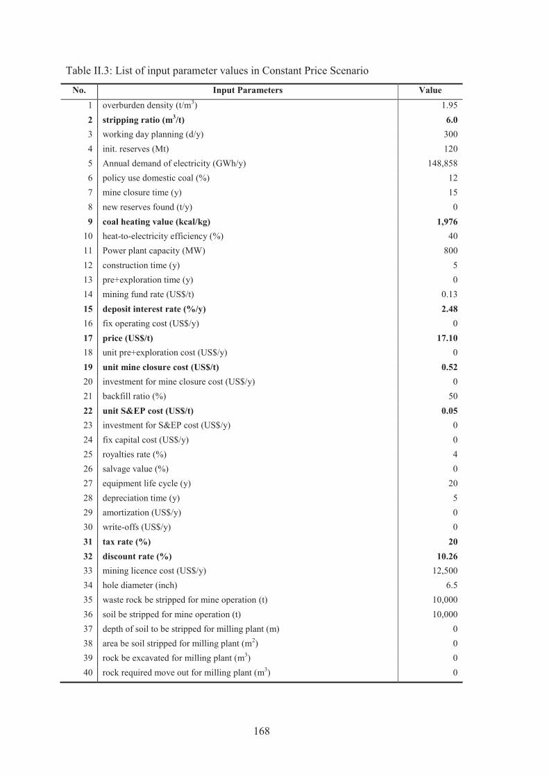
168
Table II.3: List of input parameter values in Constant Price Scenario
No. Input Parameters Value 1 overburden density (t/m3) 1.95 2 stripping ratio (m3/t) 6.0 3 working day planning (d/y) 300 4 init. reserves (Mt) 120 5 Annual demand of electricity (GWh/y) 148,858 6 policy use domestic coal (%) 12 7 mine closure time (y) 15 8 new reserves found (t/y) 0 9 coal heating value (kcal/kg) 1,976
10 heat-to-electricity efficiency (%) 40 11 Power plant capacity (MW) 800 12 construction time (y) 5 13 pre+exploration time (y) 0 14 mining fund rate (US$/t) 0.13 15 deposit interest rate (%/y) 2.48 16 fix operating cost (US$/y) 0 17 price (US$/t) 17.10 18 unit pre+exploration cost (US$/y) 0 19 unit mine closure cost (US$/t) 0.52 20 investment for mine closure cost (US$/y) 0 21 backfill ratio (%) 50 22 unit S&EP cost (US$/t) 0.05 23 investment for S&EP cost (US$/y) 0 24 fix capital cost (US$/y) 0 25 royalties rate (%) 4 26 salvage value (%) 0 27 equipment life cycle (y) 20 28 depreciation time (y) 5 29 amortization (US$/y) 0 30 write-offs (US$/y) 0 31 tax rate (%) 20 32 discount rate (%) 10.26 33 mining licence cost (US$/y) 12,500 34 hole diameter (inch) 6.5 35 waste rock be stripped for mine operation (t) 10,000 36 soil be stripped for mine operation (t) 10,000 37 depth of soil to be stripped for milling plant (m) 0 38 area be soil stripped for milling plant (m2) 0 39 rock be excavated for milling plant (m3) 0 40 rock required move out for milling plant (m3) 0
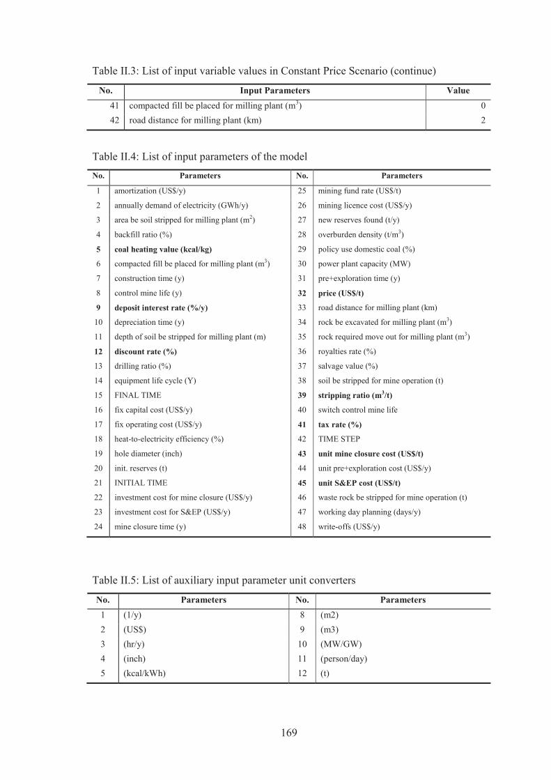
169
Table II.3: List of input variable values in Constant Price Scenario (continue)
No. Input Parameters Value 41 compacted fill be placed for milling plant (m3) 0 42 road distance for milling plant (km) 2
Table II.4: List of input parameters of the model No. Parameters No. Parameters
1 amortization (US$/y) 25 mining fund rate (US$/t)
2 annually demand of electricity (GWh/y) 26 mining licence cost (US$/y)
3 area be soil stripped for milling plant (m2) 27 new reserves found (t/y)
4 backfill ratio (%) 28 overburden density (t/m3)
5 coal heating value (kcal/kg) 29 policy use domestic coal (%)
6 compacted fill be placed for milling plant (m3) 30 power plant capacity (MW)
7 construction time (y) 31 pre+exploration time (y)
8 control mine life (y) 32 price (US$/t)
9 deposit interest rate (%/y) 33 road distance for milling plant (km)
10 depreciation time (y) 34 rock be excavated for milling plant (m3)
11 depth of soil be stripped for milling plant (m) 35 rock required move out for milling plant (m3)
12 discount rate (%) 36 royalties rate (%)
13 drilling ratio (%) 37 salvage value (%)
14 equipment life cycle (Y) 38 soil be stripped for mine operation (t)
15 FINAL TIME 39 stripping ratio (m3/t)
16 fix capital cost (US$/y) 40 switch control mine life
17 fix operating cost (US$/y) 41 tax rate (%)
18 heat-to-electricity efficiency (%) 42 TIME STEP
19 hole diameter (inch) 43 unit mine closure cost (US$/t)
20 init. reserves (t) 44 unit pre+exploration cost (US$/y)
21 INITIAL TIME 45 unit S&EP cost (US$/t)
22 investment cost for mine closure (US$/y) 46 waste rock be stripped for mine operation (t)
23 investment cost for S&EP (US$/y) 47 working day planning (days/y)
24 mine closure time (y) 48 write-offs (US$/y)
Table II.5: List of auxiliary input parameter unit converters
No. Parameters No. Parameters 1 (1/y) 8 (m2) 2 (US$) 9 (m3) 3 (hr/y) 10 (MW/GW) 4 (inch) 11 (person/day) 5 (kcal/kWh) 12 (t)
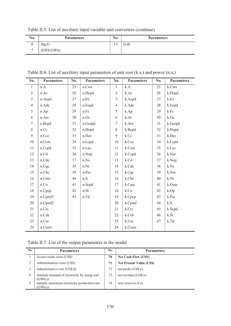
170
Table II.5: List of auxiliary input variable unit converters (continue)
No. Parameters No. Parameters 6 (kg/t) 13 (t/d) 7 (kWh/GWh)
Table II.6: List of auxiliary input parameters of unit cost (k.xi) and power (n.xi)
No. Parameters No. Parameters No. Parameters No. Parameters 1 n.A 25 n.Cws 1 k.A 25 k.Cws 2 n.Ac 26 n.Dcpd 2 k.Ac 26 k.Dcpd 3 n.Acpd 27 n.Ec 3 k.Acpd 27 k.Ec 4 n.Adc 28 n.Ecpd 4 k.Adc 28 k.Ecpd 5 n.Ap 29 n.Fc 5 k.Ap 29 k.Fc 6 n.Ars 30 n.Gc 6 k.Ar 30 k.Gc 7 n.Bcpd 31 n.Gscpd 7 k.Ars 31 k.Gscpd 8 n.Cc 32 n.Hcpd 8 k.Bcpd 32 k.Hcpd 9 n.Cce 33 n.Hec 9 k.Cc 33 k.Hec 10 n.Ccm 34 n.Lcpd 10 k.Cce 34 k.Lcpd 11 n.Ccpd 35 n.Lec 11 k.Ccm 35 k.Lec 12 n.Cd 36 n.Nop 12 k.Ccpd 36 k.Nat 13 n.Cde 37 n.Ns 13 k.Cd 37 k.Nop 14 n.Cgc 38 n.Nt 14 k.Cde 38 k.Ns 15 n.Chc 39 n.Psc 15 k.Cgc 39 k.Nsv 16 n.Cme 40 n.S 16 k.Chc 40 k.Nt 17 n.Co 41 n.Scpd 17 k.Cme 41 k.Ome 18 n.Cpcp 42 n.St 18 k.Co 42 k.Op 19 n.Cpmf1 43 n.Td 19 k.Cpcp 43 k.Psc 20 n.Cpmf2 20 k.Cpmf 44 k.S 21 n.Crs 21 k.Crs 45 k.Scpd 22 n.Csh 22 k.Csh 46 k.St 23 n.Css 23 k.Css 47 k.Td 24 n.Cssm 24 k.Cssm
Table II.7: List of the output parameters in the model No. Parameters No. Parameters
1 Access roads costs (US$) 70 Net Cash Flow (US$)
2 Administration costs (US$) 71 Net Present Value (US$)
3 Administrative cost (US$/d) 72 net profit (US$/y)
4 Annualy demand of electricity by using coal (GWh/y)
73 net revenue (US$/y)
5 annualy maximum electricity production rate (GWh/y)
74 new reserves (t/y)
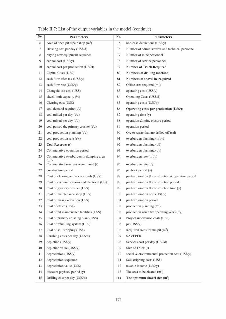
171
Table II.7: List of the output variables in the model (continue) No. Parameters No. Parameters
6 Area of open pit repair shop (m2) 75 non-cash deductions (US$/y)
7 Blasting cost per day (US$/d) 76 Number of administrative and technical personnel
8 buying new equipment sequence 77 Number of mine personnel
9 capital cost (US$/y) 78 Number of service personnel
10 capital cost per production (US$/t) 79 Number of Truck Required
11 Capital Costs (US$) 80 Numbers of drilling machine
12 cash flow after-tax (US$/y) 81 Numbers of shovel be required
13 cash flow rate (US$/y) 82 Office area required (m2)
14 Changehouse cost (US$) 83 operating cost (US$/y)
15 check limit capacity (%) 84 Operating Costs (US$/d)
16 Clearing cost (US$) 85 operating costs (US$/y)
17 coal demand require (t/y) 86 Operating costs per production (US$/t)
18 coal milled per day (t/d) 87 operating time (y)
19 coal mined per day (t/d) 88 operation & mine closure period
20 coal passed the primary crusher (t/d) 89 operation period
21 coal production planning (t/y) 90 Ore or waste that are drilled off (t/d)
22 coal production rate (t/y) 91 overburden planning (m3/y)
23 Coal Reserves (t) 92 overburden planning (t/d)
24 Commutative operation period 93 overburden planning (t/y)
25 Commutative overburden in dumping area (m3)
94 overburden rate (m3/y)
26 Commutative reserves were mined (t) 95 overburden rate (t/y)
27 construction period 96 payback period (y)
28 Cost of clearing and access roads (US$) 97 pre+exploration & construction & operation period
29 Cost of communications and electrical (US$) 98 pre+exploration & construction period
30 Cost of gyratory crusher (US$) 99 pre+exploration & construction time (y)
31 Cost of maintenance shop (US$) 100 pre+exploration cost (US$/y)
32 Cost of mass excavation (US$) 101 pre+exploration period
33 Cost of office (US$) 102 production planning (t/d)
34 Cost of pit maintenance facilities (US$) 103 production when fix operating years (t/y)
35 Cost of primary crushing plant (US$) 104 Project supervision costs (US$)
36 Cost of refuelling system (US$) 105 pv (US$/y)
37 Cost of soil stripping (US$) 106 Required areas for the pit (m2)
38 Crushing costs per day (US$/d) 107 SAVEPER
39 depletion (US$/y) 108 Services cost per day (US$/d)
40 depletion value (US$/y) 109 Size of Truck (t)
41 depreciation (US$/y) 110 social & environmental protection cost (US$/y)
42 depreciation sequence 111 Soil stripping costs (US$)
43 depreciation value (US$) 112 taxable income (US$/y)
44 discount payback period (y) 113 The area to be cleared (m2)
45 Drilling cost per day (US$/d) 114 The optimum shovel size (m3)
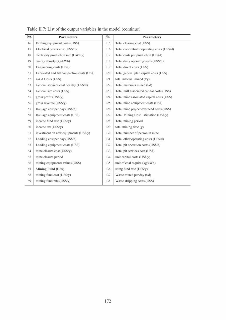
172
Table II.7: List of the output variables in the model (continue) No. Parameters No. Parameters
46 Drilling equipment costs (US$) 115 Total clearing cost (US$)
47 Electrical power cost (US$/d) 116 Total concentrator operating costs (US$/d)
48 electricity production rate (GWh/y) 117 Total costs per production (US$/t)
49 energy density (kg/kWh) 118 Total daily operating costs (US$/d)
50 Engineering costs (US$) 119 Total direct costs (US$)
51 Excavated and fill compaction costs (US$) 120 Total general plan capital costs (US$)
52 G&A Costs (US$) 121 total material mined (t/y)
53 General services cost per day (US$/d) 122 Total materials mined (t/d)
54 General site costs (US$) 123 Total mill associated capital costs (US$)
55 gross profit (US$/y) 124 Total mine associated capital costs (US$)
56 gross revenue (US$/y) 125 Total mine equipment costs (US$)
57 Haulage cost per day (US$/d) 126 Total mine project overhead costs (US$)
58 Haulage equipment costs (US$) 127 Total Mining Cost Estimation (US$/y)
59 income fund rate (US$/y) 128 Total mining period
60 income tax (US$/y) 129 total mining time (y)
61 investment on new equipments (US$/y) 130 Total number of person in mine
62 Loading cost per day (US$/d) 131 Total other operating costs (US$/d)
63 Loading equipment costs (US$) 132 Total pit operation costs (US$/d)
64 mine closure cost (US$/y) 133 Total pit services cost (US$)
65 mine closure period 134 unit capital costs (US$/y)
66 mining equipments values (US$) 135 unit of coal require (kg/kWh)
67 Mining Fund (US$) 136 using fund rate (US$/y)
68 mining fund cost (US$/y) 137 Waste mined per day (t/d)
69 mining fund rate (US$/y) 138 Waste stripping costs (US$)
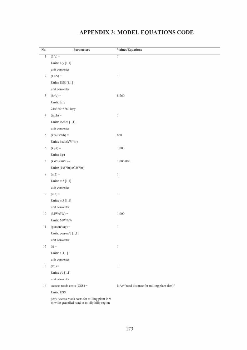
173
III. APPENDIX 3: MODEL EQUATIONS CODE No. Parameters Values/Equations
1 (1/y) = 1
Units: 1/y [1,1]
unit converter
2 (US$) = 1
Units: US$ [1,1]
unit converter
3 (hr/y) = 8,760
Units: hr/y
24x365=8760 hr/y
4 (inch) = 1
Units: inches [1,1]
unit converter
5 (kcal/kWh) = 860
Units: kcal/(kW*hr)
6 (kg/t) = 1,000
Units: kg/t
7 (kWh/GWh) = 1,000,000
Units: (kW*hr)/(GW*hr)
8 (m2) = 1
Units: m2 [1,1]
unit converter
9 (m3) = 1
Units: m3 [1,1]
unit converter
10 (MW/GW) = 1,000
Units: MW/GW
11 (person/day) = 1
Units: person/d [1,1]
unit converter
12 (t) = 1
Units: t [1,1]
unit converter
13 (t/d) = 1
Units: t/d [1,1]
unit converter
14 Access roads costs (US$) = k.Ar*"road distance for milling plant (km)"
Units: US$
(Ar) Access roads costs for milling plant in 9 m wide gravelled road in mildly hilly region
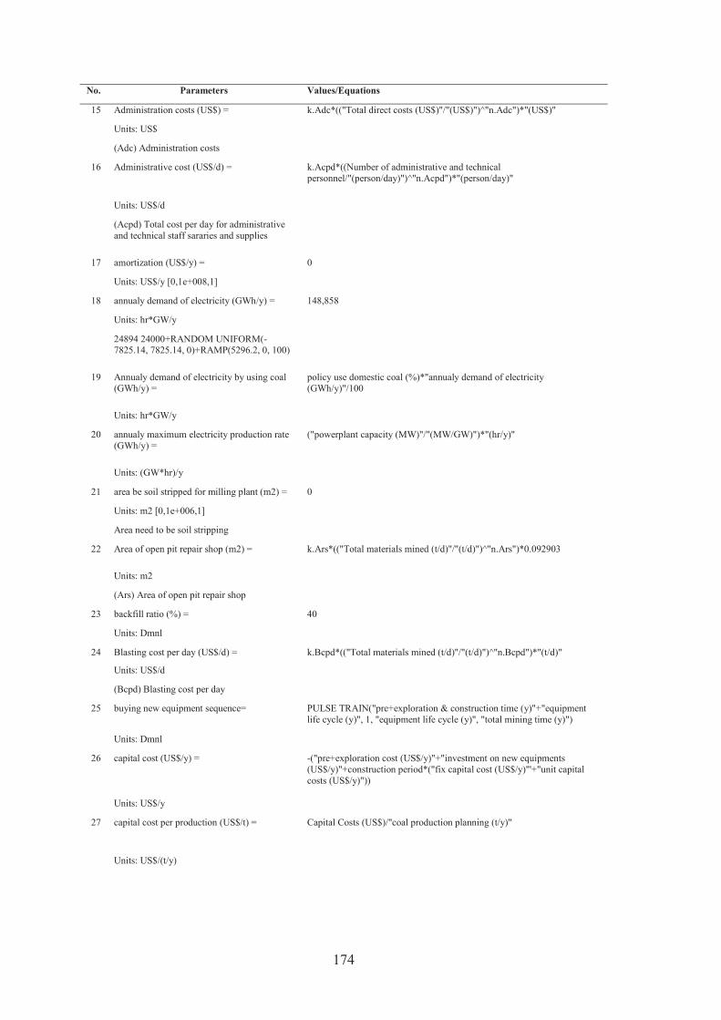
174
No. Parameters Values/Equations
15 Administration costs (US$) = k.Adc*(("Total direct costs (US$)"/"(US$)")^"n.Adc")*"(US$)"
Units: US$
(Adc) Administration costs
16 Administrative cost (US$/d) = k.Acpd*((Number of administrative and technical personnel/"(person/day)")^"n.Acpd")*"(person/day)"
Units: US$/d
(Acpd) Total cost per day for administrative and technical staff sararies and supplies
17 amortization (US$/y) = 0
Units: US$/y [0,1e+008,1]
18 annualy demand of electricity (GWh/y) = 148,858
Units: hr*GW/y
24894 24000+RANDOM UNIFORM(-7825.14, 7825.14, 0)+RAMP(5296.2, 0, 100)
19 Annualy demand of electricity by using coal (GWh/y) =
policy use domestic coal (%)*"annualy demand of electricity (GWh/y)"/100
Units: hr*GW/y
20 annualy maximum electricity production rate (GWh/y) =
("powerplant capacity (MW)"/"(MW/GW)")*"(hr/y)"
Units: (GW*hr)/y
21 area be soil stripped for milling plant (m2) = 0
Units: m2 [0,1e+006,1]
Area need to be soil stripping
22 Area of open pit repair shop (m2) = k.Ars*(("Total materials mined (t/d)"/"(t/d)")^"n.Ars")*0.092903
Units: m2
(Ars) Area of open pit repair shop
23 backfill ratio (%) = 40
Units: Dmnl
24 Blasting cost per day (US$/d) = k.Bcpd*(("Total materials mined (t/d)"/"(t/d)")^"n.Bcpd")*"(t/d)"
Units: US$/d
(Bcpd) Blasting cost per day
25 buying new equipment sequence= PULSE TRAIN("pre+exploration & construction time (y)"+"equipment life cycle (y)", 1, "equipment life cycle (y)", "total mining time (y)")
Units: Dmnl
26 capital cost (US$/y) = -("pre+exploration cost (US$/y)"+"investment on new equipments (US$/y)"+construction period*("fix capital cost (US$/y)"'+"unit capital costs (US$/y)"))
Units: US$/y
27 capital cost per production (US$/t) = Capital Costs (US$)/"coal production planning (t/y)"
Units: US$/(t/y)
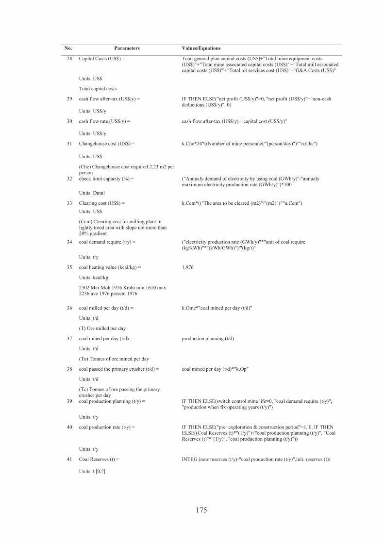
175
No. Parameters Values/Equations
28 Capital Costs (US$) = Total general plan capital costs (US$)+"Total mine equipment costs (US$)"+"Total mine associated capital costs (US$)"'+"Total mill associated capital costs (US$)"'+"Total pit services cost (US$)"+"G&A Costs (US$)"
Units: US$
Total capital costs
29 cash flow after-tax (US$/y) = IF THEN ELSE("net profit (US$/y)">0, "net profit (US$/y)"+"non-cash deductions (US$/y)", 0)
Units: US$/y
30 cash flow rate (US$/y) = cash flow after-tax (US$/y)+"capital cost (US$/y)"
Units: US$/y
31 Changehouse cost (US$) = k.Chc*24*((Number of mine personnel/"(person/day)")^"n.Chc")
Units: US$
(Chc) Changehouse cost required 2.23 m2 per person
32 check limit capacity (%) = ("Annualy demand of electricity by using coal (GWh/y)"/"annualy maximum electricity production rate (GWh/y)")*100
Units: Dmnl
33 Clearing cost (US$) = k.Ccm*(("The area to be cleared (m2)"/"(m2)")^"n.Ccm") Units: US$
(Ccm) Clearing cost for milling plant in lightly treed area with slope not more than 20% gradient
34 coal demand require (t/y) = ("electricity production rate (GWh/y)"*"unit of coal require (kg/kWh)"*"(kWh/GWh)")/"(kg/t)"
Units: t/y
35 coal heating value (kcal/kg) = 1,976
Units: kcal/kg
2502 Mar Moh 1976 Krabi min 1610 max 2236 ave 1976 present 1976
36 coal milled per day (t/d) = k.Ome*"coal mined per day (t/d)"
Units: t/d
(T) Ore milled per day
37 coal mined per day (t/d) = production planning (t/d)
Units: t/d
(To) Tonnes of ore mined per day
38 coal passed the primary crusher (t/d) = coal mined per day (t/d)*"k.Op"
Units: t/d
(Tc) Tonnes of ore passing the primary crusher per day
39 coal production planning (t/y) = IF THEN ELSE(switch control mine life=0, "coal demand require (t/y)", "production when fix operating years (t/y)")
Units: t/y
40 coal production rate (t/y) = IF THEN ELSE("pre+exploration & construction period"=1, 0, IF THEN ELSE((Coal Reserves (t)*"(1/y)")<"coal production planning (t/y)", "Coal Reserves (t)"*"(1/y)", "coal production planning (t/y)"))
Units: t/y
41 Coal Reserves (t) = INTEG (new reserves (t/y)-"coal production rate (t/y)",init. reserves (t))
Units: t [0,?]
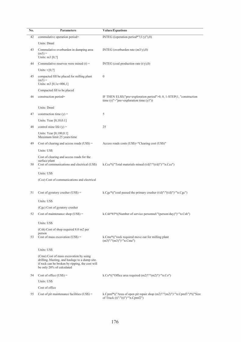
176
No. Parameters Values/Equations
42 commulative operation period= INTEG ((operation period*"(1/y)"),0)
Units: Dmnl
43 Commulative overburden in dumping area (m3) =
INTEG (overburden rate (m3/y),0)
Units: m3 [0,?]
44 Commulative reserves were mined (t) = INTEG (coal production rate (t/y),0)
Units: t [0,?]
45 compacted fill be placed for milling plant (m3) =
0
Units: m3 [0,1e+006,1]
Compacted fill to be placed
46 construction period= IF THEN ELSE("pre+exploration period">0, 0, 1-STEP(1, "construction time (y)"+"pre+exploration time (y)"))
Units: Dmnl
47 construction time (y) = 5
Units: Year [0,10,0.1]
48 control mine life (y) = 25
Units: Year [0,100,0.1] Maximum limit 25 years/time
49 Cost of clearing and access roads (US$) = Access roads costs (US$)+"Clearing cost (US$)"
Units: US$
Cost of clearing and access roads for the surface plant
50 Cost of communications and electrical (US$) =
k.Cce*(("Total materials mined (t/d)"/"(t/d)")^"n.Cce")
Units: US$
(Cce) Cost of communications and electrical
51 Cost of gyratory crusher (US$) = k.Cgc*(("coal passed the primary crusher (t/d)"/"(t/d)")^"n.Cgc")
Units: US$
(Cgc) Cost of gyratory crusher
52 Cost of maintenance shop (US$) = k.Csh*85*((Number of service personnel/"(person/day)")^"n.Csh")
Units: US$
(Csh) Cost of shop required 8.0 m2 per person
53 Cost of mass excavation (US$) = k.Cme*(("rock required move out for milling plant (m3)"/"(m3)")^"n.Cme")
Units: US$
(Cme) Cost of mass excavation by using drilling, blasting, and haulage to a dump site. if rock can be broken by ripping, the cost will be only 20% of calculated
54 Cost of office (US$) = k.Co*(("Office area required (m2)"/"(m2)")^"n.Co")
Units: US$
Cost of office
55 Cost of pit maintenance facilities (US$) = k.Cpmf*(("Area of open pit repair shop (m2)"/"(m2)")^"n.Cpmf1")*(("Size of Truck (t)"/"(t)")^"n.Cpmf2")

177
No. Parameters Values/Equations
Units: US$
(Cpmf) Cost of pit maintenance facilities
56 Cost of primary crushing plant (US$) = k.Cpcp*(("coal passed the primary crusher (t/d)"/"(t/d)")^"n.Cpcp")
Units: US$
(Cpcp) Cost of primary crushing plant
57 Cost of refueling system (US$) = k.Crs*(("Total materials mined (t/d)"/"(t/d)")^"n.Crs")
Units: US$
(Crs) Cost of refueling system
58 Cost of soil stripping (US$) = k.Cssm*(("area be soil stripped for milling plant (m2)"/"(m2)")^"n.Cssm")*"depth of soil be stripped for milling plant (m)"
Units: US$
(Cssm) Cost of soil stripping for milling plant construction
59 Crushing costs per day (US$/d) = k.Ccpd*(("coal passed the primary crusher (t/d)"/"(t/d)")^"n.Ccpd")*"(t/d)"
Units: US$/d
(Ccpd) Crushing costs per day
60 depletion (US$/y) = IF THEN ELSE(operation period>0, "depletion value (US$/y)", 0) Units: US$/y
61 depletion value (US$/y) = mining licence cost (US$/y)
Units: US$/y [0,1e+009,1]
62 deposit interest rate (%/y) = 2
Units: 1/y [0,100,0.01]
min 1.25 max 5.0 ave 2.48 present 2.25
63 depreciation (US$/y) = IF THEN ELSE(operation period>0, ("depreciation value (US$)"/"depreciation time (y)")*depreciation sequence, 0)
Units: US$/y
64 depreciation sequence= PULSE TRAIN("pre+exploration & construction time (y)", "depreciation time (y)", "equipment life cycle (Y)", "total mining time (y)")
Units: Dmnl
65 depreciation time (y) = 5
Units: Year [0,50,0.1]
66 depreciation value (US$) = ((100-"salvage value (%)")/100)*"mining equipments values (US$)"
Units: US$
67 depth of soil be stripped for milling plant (m) =
0
Units: m [0,100,1]
Depth of soil to be stripped
68 discount payback period (y) = IF THEN ELSE("Net Present Value (US$)">0, 1, 0)
Units: Dmnl [?,1]
69 discount rate (%) = 10
Units: Dmnl [0,100,0.01]
min 4.7 max 15.9 ave 10.26 present 10.26
70 Drilling cost per day (US$/d) = k.Dcpd*(("Total materials mined (t/d)"/"(t/d)")^"n.Dcpd")*"(t/d)"
Units: US$/d

178
No. Parameters Values/Equations
(Dcpd) Drilling cost per day
71 Drilling equipment costs (US$) = Numbers of drilling machine*"k.Cde"*(("hole diameter (inch)"/"(inch)")^"n.Cde")
Units: US$
(Cde) Drilling equipment costs, included 25% allowance for drilling and blasting supplies and accessory equipment
72 drilling ratio (%) = 60
Units: Dmnl [0,100,1]
ratio of area need drilling machine for production
73 Electrical power cost (US$/d) = k.Ecpd*(("coal milled per day (t/d)"/"(t/d)")^"n.Ecpd")*"(t/d)"
Units: US$/d
(Ecpd) Electrical power cost (US$/d)
74 electricity production rate (GWh/y) = IF THEN ELSE("check limit capacity (%)"<=100, "check limit capacity (%)"*annualy maximum electricity production rate (GWh/y)/100, "annualy maximum electricity production rate (GWh/y)")
Units: (GW*hr)/y
75 energy density (kg/kWh) = (kcal/kWh)/"coal heating value (kcal/kg)"
Units: kg/(hr*kW)
76 Engineering costs (US$) = k.Ec*(("Total direct costs (US$)"/"(US$)")^"n.Ec")*"(US$)"
Units: US$
(Ec) Engineering costs
77 equipment life cycle (Y) = 20
Units: Year [1,25,1]
78 Excavated and fill compaction costs (US$) = k.Cd*(("rock be excavated for milling plant (m3)"/"(m3)")^"n.Cd")+"k.Fc"*(("compacted fill be placed for milling plant (m3)"/"(m3)")^"n.Fc")
Units: US$
Excavated and fill compaction costs
79 FINAL TIME = 100
Units: Year [0,100,0.1]
The final time for the simulation.
80 fix capital cost (US$/y) = 0
Units: US$/y
81 fix operating cost (US$/y) = 0
Units: US$/y [0,1e+008,1]
82 G&A Costs (US$) = Total mine project overhead costs (US$)
Units: US$
Total general and administrative costs
83 General services cost per day (US$/d) = k.Gscpd*(("Total materials mined (t/d)"/"(t/d)")^"n.Gscpd")*"(t/d)"
Units: US$/d
(Gscpd)General services cost per day
84 General site costs (US$) = k.Gc*(("Total direct costs (US$)"/"(US$)")^"n.Gc")*"(US$)"
Units: US$
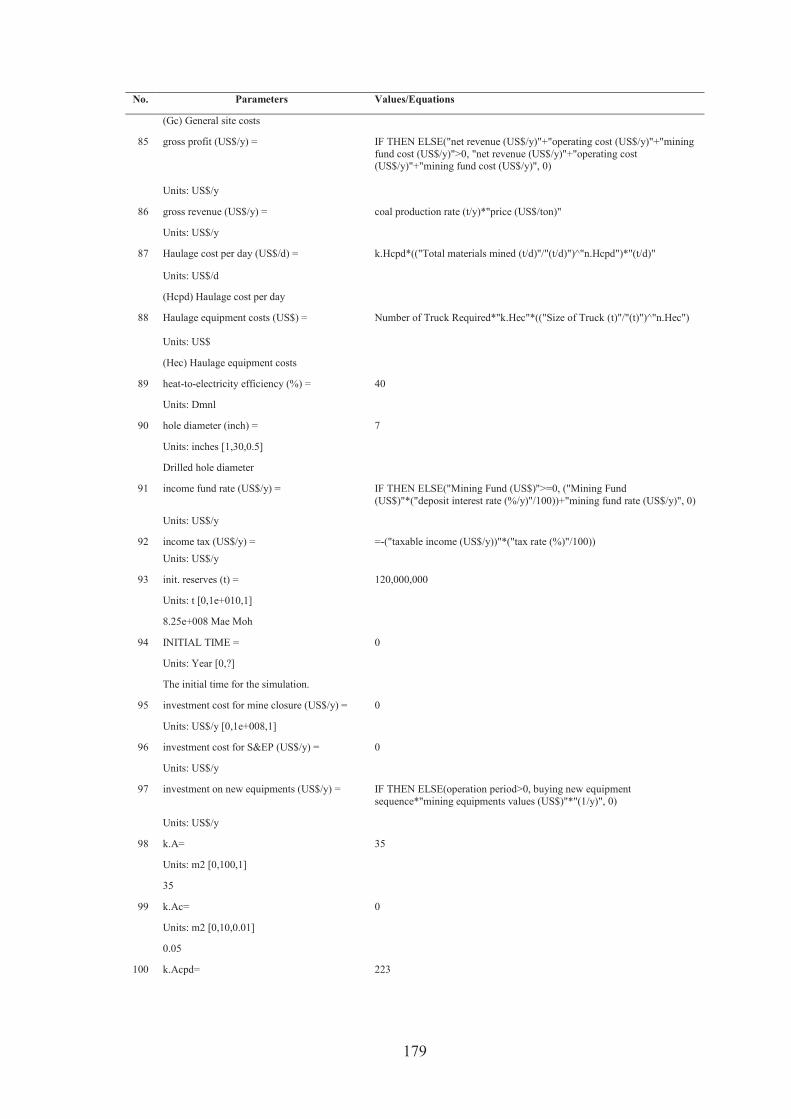
179
No. Parameters Values/Equations
(Gc) General site costs
85 gross profit (US$/y) = IF THEN ELSE("net revenue (US$/y)"+"operating cost (US$/y)"+"mining fund cost (US$/y)">0, "net revenue (US$/y)"+"operating cost (US$/y)"+"mining fund cost (US$/y)", 0)
Units: US$/y
86 gross revenue (US$/y) = coal production rate (t/y)*"price (US$/ton)"
Units: US$/y
87 Haulage cost per day (US$/d) = k.Hcpd*(("Total materials mined (t/d)"/"(t/d)")^"n.Hcpd")*"(t/d)"
Units: US$/d
(Hcpd) Haulage cost per day
88 Haulage equipment costs (US$) = Number of Truck Required*"k.Hec"*(("Size of Truck (t)"/"(t)")^"n.Hec")
Units: US$
(Hec) Haulage equipment costs
89 heat-to-electricity efficiency (%) = 40
Units: Dmnl
90 hole diameter (inch) = 7
Units: inches [1,30,0.5]
Drilled hole diameter
91 income fund rate (US$/y) = IF THEN ELSE("Mining Fund (US$)">=0, ("Mining Fund (US$)"*("deposit interest rate (%/y)"/100))+"mining fund rate (US$/y)", 0)
Units: US$/y
92 income tax (US$/y) = =-("taxable income (US$/y))"*("tax rate (%)"/100)) Units: US$/y
93 init. reserves (t) = 120,000,000
Units: t [0,1e+010,1]
8.25e+008 Mae Moh
94 INITIAL TIME = 0
Units: Year [0,?]
The initial time for the simulation.
95 investment cost for mine closure (US$/y) = 0
Units: US$/y [0,1e+008,1]
96 investment cost for S&EP (US$/y) = 0
Units: US$/y
97 investment on new equipments (US$/y) = IF THEN ELSE(operation period>0, buying new equipment sequence*"mining equipments values (US$)"*"(1/y)", 0)
Units: US$/y
98 k.A= 35
Units: m2 [0,100,1]
35
99 k.Ac= 0
Units: m2 [0,10,0.01]
0.05
100 k.Acpd= 223
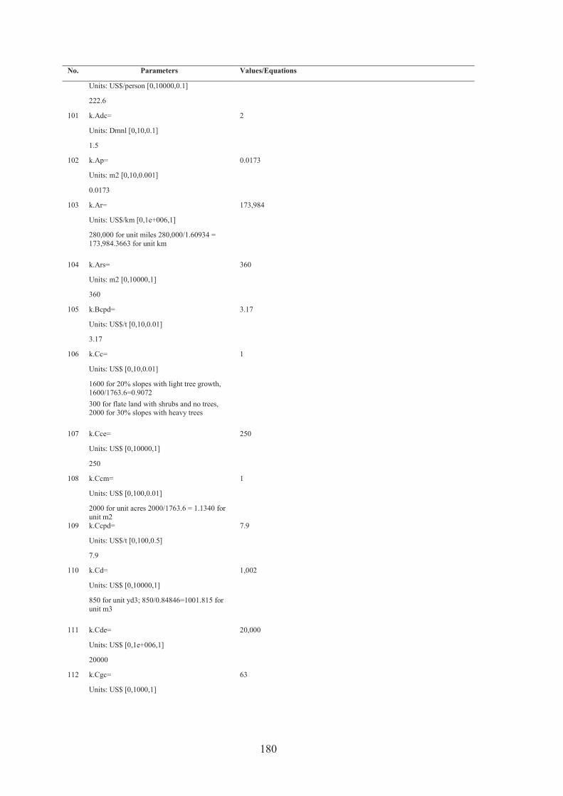
180
No. Parameters Values/Equations
Units: US$/person [0,10000,0.1]
222.6
101 k.Adc= 2
Units: Dmnl [0,10,0.1]
1.5
102 k.Ap= 0.0173
Units: m2 [0,10,0.001]
0.0173
103 k.Ar= 173,984
Units: US$/km [0,1e+006,1]
280,000 for unit miles 280,000/1.60934 = 173,984.3663 for unit km
104 k.Ars= 360
Units: m2 [0,10000,1]
360
105 k.Bcpd= 3.17
Units: US$/t [0,10,0.01]
3.17
106 k.Cc= 1
Units: US$ [0,10,0.01]
1600 for 20% slopes with light tree growth, 1600/1763.6=0.9072
300 for flate land with shrubs and no trees, 2000 for 30% slopes with heavy trees
107 k.Cce= 250
Units: US$ [0,10000,1]
250
108 k.Ccm= 1
Units: US$ [0,100,0.01]
2000 for unit acres 2000/1763.6 = 1.1340 for unit m2
109 k.Ccpd= 7.9
Units: US$/t [0,100,0.5]
7.9
110 k.Cd= 1,002
Units: US$ [0,10000,1]
850 for unit yd3; 850/0.84846=1001.815 for unit m3
111 k.Cde= 20,000
Units: US$ [0,1e+006,1]
20000
112 k.Cgc= 63
Units: US$ [0,1000,1]
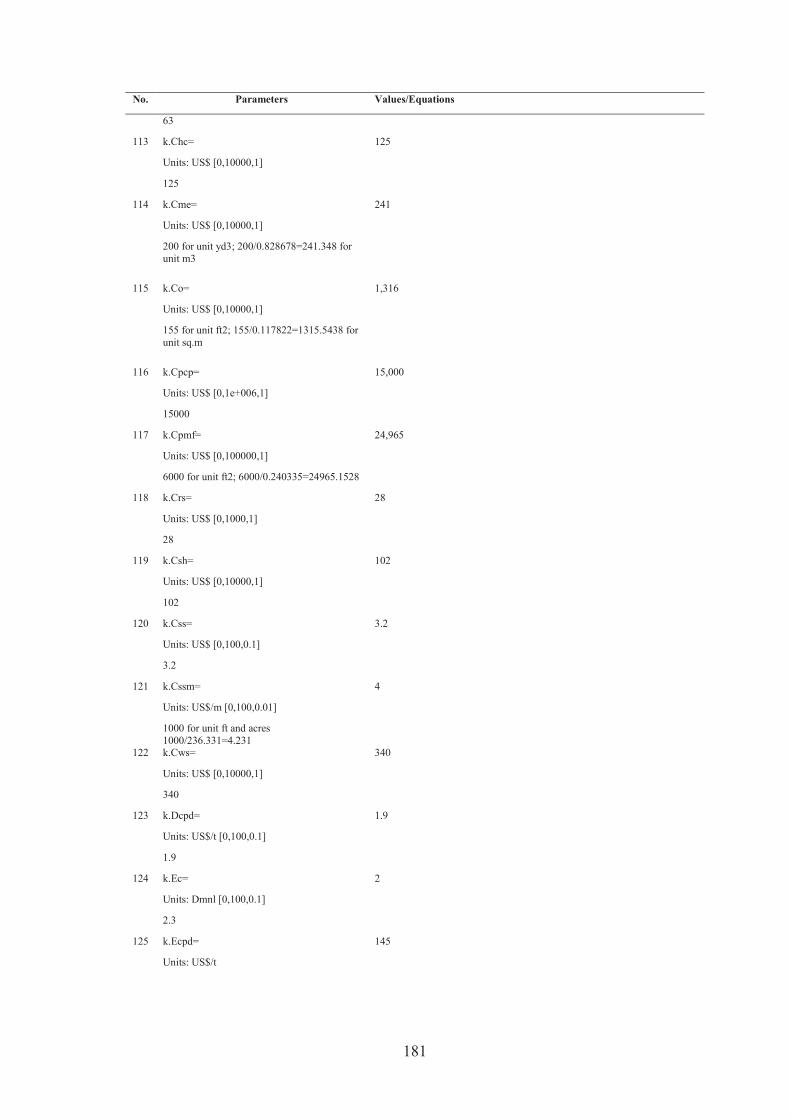
181
No. Parameters Values/Equations
63
113 k.Chc= 125
Units: US$ [0,10000,1]
125
114 k.Cme= 241
Units: US$ [0,10000,1]
200 for unit yd3; 200/0.828678=241.348 for unit m3
115 k.Co= 1,316
Units: US$ [0,10000,1]
155 for unit ft2; 155/0.117822=1315.5438 for unit sq.m
116 k.Cpcp= 15,000
Units: US$ [0,1e+006,1]
15000
117 k.Cpmf= 24,965
Units: US$ [0,100000,1]
6000 for unit ft2; 6000/0.240335=24965.1528
118 k.Crs= 28
Units: US$ [0,1000,1]
28
119 k.Csh= 102
Units: US$ [0,10000,1]
102
120 k.Css= 3.2
Units: US$ [0,100,0.1]
3.2
121 k.Cssm= 4
Units: US$/m [0,100,0.01]
1000 for unit ft and acres 1000/236.331=4.231
122 k.Cws= 340
Units: US$ [0,10000,1]
340
123 k.Dcpd= 1.9
Units: US$/t [0,100,0.1]
1.9
124 k.Ec= 2
Units: Dmnl [0,100,0.1]
2.3
125 k.Ecpd= 145
Units: US$/t
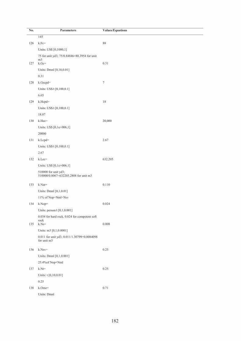
182
No. Parameters Values/Equations
145
126 k.Fc= 88
Units: US$ [0,1000,1]
75 for unit yd3; 75/0.84846=88.3954 for unit m3
127 k.Gc= 0.31
Units: Dmnl [0,10,0.01]
0.31
128 k.Gscpd= 7
Units: US$/t [0,100,0.1]
6.65
129 k.Hcpd= 18
Units: US$/t [0,100,0.1]
18.07
130 k.Hec= 20,000
Units: US$ [0,1e+006,1]
20000
131 k.Lcpd= 2.67
Units: US$/t [0,100,0.1]
2.67
132 k.Lec= 632,205
Units: US$ [0,1e+006,1]
510000 for unit yd3; 510000/0.8067=632205.2808 for unit m3
133 k.Nat= 0.110
Units: Dmnl [0,1,0.01]
11% of Nop+Nml+Nsv
134 k.Nop= 0.024
Units: person/t [0,1,0.001]
0.034 for hard rock, 0.024 for competent soft rock
135 k.Ns= 0.008
Units: m3 [0,1,0.0001]
0.011 for unit yd3; 0.011/1.30799=0.0084098 for unit m3
136 k.Nsv= 0.25
Units: Dmnl [0,1,0.001]
25.4%of Nop+Nml
137 k.Nt= 0.25
Units: t [0,10,0.01]
0.25
138 k.Ome= 0.71
Units: Dmnl
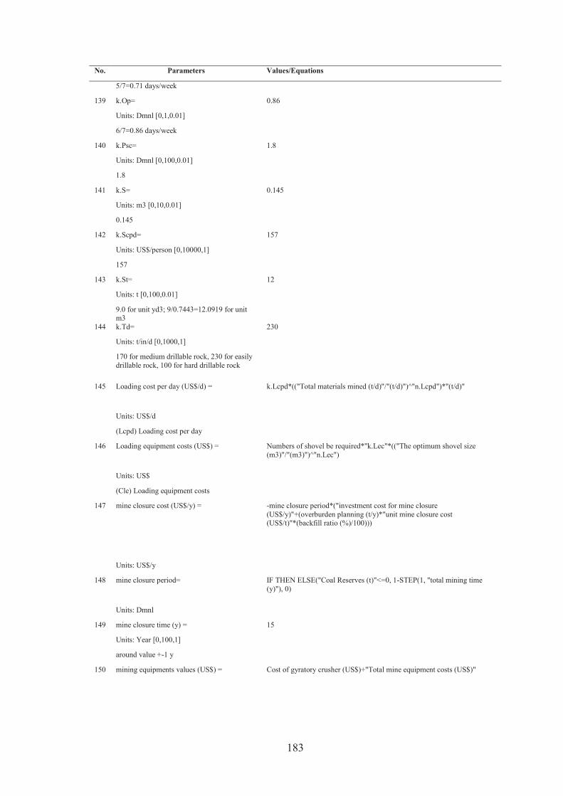
183
No. Parameters Values/Equations
5/7=0.71 days/week
139 k.Op= 0.86
Units: Dmnl [0,1,0.01]
6/7=0.86 days/week
140 k.Psc= 1.8
Units: Dmnl [0,100,0.01]
1.8
141 k.S= 0.145
Units: m3 [0,10,0.01]
0.145
142 k.Scpd= 157
Units: US$/person [0,10000,1]
157
143 k.St= 12
Units: t [0,100,0.01]
9.0 for unit yd3; 9/0.7443=12.0919 for unit m3
144 k.Td= 230
Units: t/in/d [0,1000,1]
170 for medium drillable rock, 230 for easily drillable rock, 100 for hard drillable rock
145 Loading cost per day (US$/d) = k.Lcpd*(("Total materials mined (t/d)"/"(t/d)")^"n.Lcpd")*"(t/d)"
Units: US$/d
(Lcpd) Loading cost per day
146 Loading equipment costs (US$) = Numbers of shovel be required*"k.Lec"*(("The optimum shovel size (m3)"/"(m3)")^"n.Lec")
Units: US$
(Cle) Loading equipment costs
147 mine closure cost (US$/y) = -mine closure period*("investment cost for mine closure (US$/y)"+(overburden planning (t/y)*"unit mine closure cost (US$/t)"*(backfill ratio (%)/100)))
Units: US$/y
148 mine closure period= IF THEN ELSE("Coal Reserves (t)"<=0, 1-STEP(1, "total mining time (y)"), 0)
Units: Dmnl
149 mine closure time (y) = 15
Units: Year [0,100,1]
around value +-1 y
150 mining equipments values (US$) = Cost of gyratory crusher (US$)+"Total mine equipment costs (US$)"
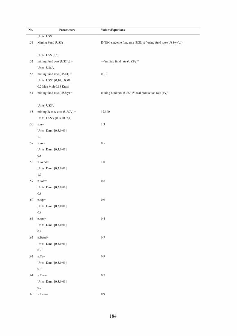
184
No. Parameters Values/Equations
Units: US$
151 Mining Fund (US$) = INTEG (income fund rate (US$/y)-"using fund rate (US$/y)",0)
Units: US$ [0,?]
152 mining fund cost (US$/y) = =-"mining fund rate (US$/y)"
Units: US$/y
153 mining fund rate (US$/t) = 0.13
Units: US$/t [0,10,0.0001]
0.2 Mae Moh 0.13 Krabi
154 mining fund rate (US$/y) = mining fund rate (US$/t)*"coal production rate (t/y)"
Units: US$/y
155 mining licence cost (US$/y) = 12,500
Units: US$/y [0,1e+007,1]
156 n.A= 1.3
Units: Dmnl [0,3,0.01]
1.3
157 n.Ac= 0.5
Units: Dmnl [0,3,0.01]
0.5
158 n.Acpd= 1.0
Units: Dmnl [0,3,0.01]
1.0
159 n.Adc= 0.8
Units: Dmnl [0,3,0.01]
0.8
160 n.Ap= 0.9
Units: Dmnl [0,3,0.01]
0.9
161 n.Ars= 0.4
Units: Dmnl [0,3,0.01]
0.4
162 n.Bcpd= 0.7
Units: Dmnl [0,3,0.01]
0.7
163 n.Cc= 0.9
Units: Dmnl [0,3,0.01]
0.9
164 n.Cce= 0.7
Units: Dmnl [0,3,0.01]
0.7
165 n.Ccm= 0.9

185
No. Parameters Values/Equations
Units: Dmnl [0,3,0.01]
0.9
166 n.Ccpd= 0.6
Units: Dmnl [0,3,0.01]
0.6
167 n.Cd= 0.6
Units: Dmnl [0,3,0.01]
0.6
168 n.Cde= 1.8
Units: Dmnl [0,3,0.01]
1.8
169 n.Cgc= 0.9
Units: Dmnl [0,3,0.01]
0.9
170 n.Chc= 0.9
Units: Dmnl [0,3,0.01]
0.9
171 n.Cme= 0.7
Units: Dmnl [0,3,0.01]
0.7
172 n.Co= 0.9
Units: Dmnl [0,3,0.01]
0.9
173 n.Cpcp= 0.7
Units: Dmnl [0,3,0.01]
0.7
174 n.Cpmf1= 0.6
Units: Dmnl [0,3,0.01]
0.6
175 n.Cpmf2= 0.1
Units: Dmnl [0,3,0.01]
0.1
176 n.Crs= 0.7
Units: Dmnl [0,3,0.01]
0.7
177 n.Csh= 0.9
Units: Dmnl [0,3,0.01]
0.9
178 n.Css= 0.8
Units: Dmnl [0,3,0.01]
0.8
179 n.Cssm= 0.8
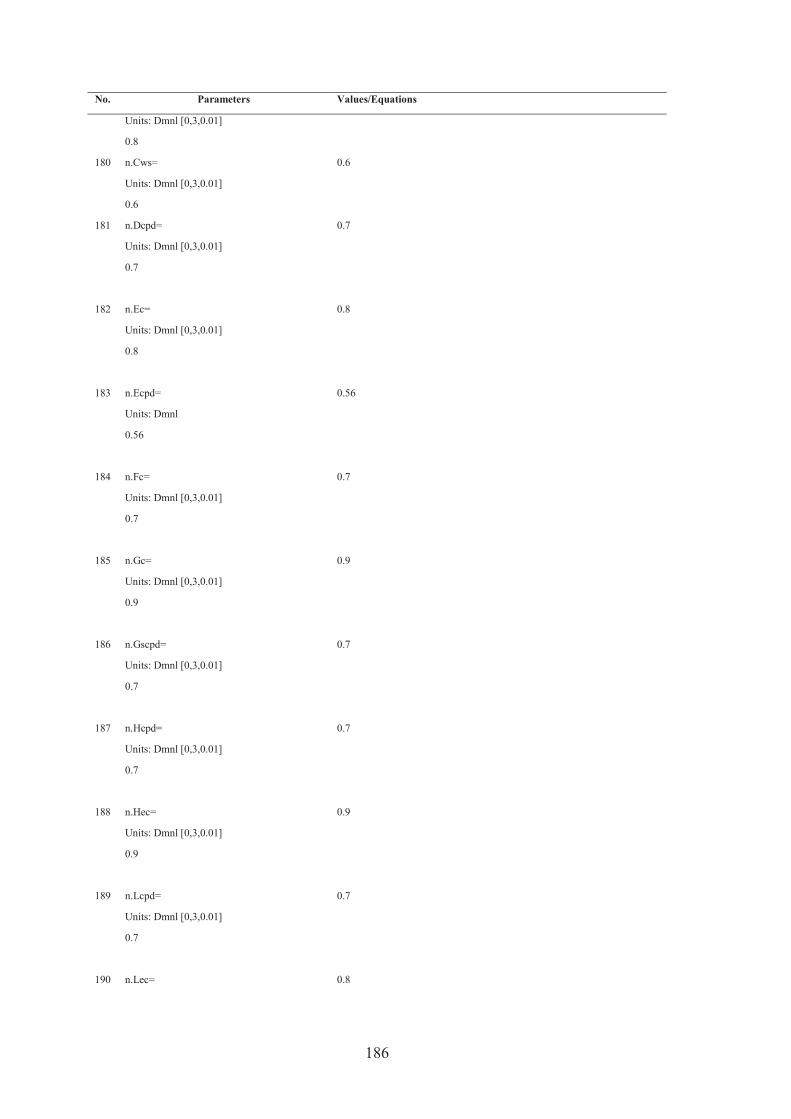
186
No. Parameters Values/Equations
Units: Dmnl [0,3,0.01]
0.8
180 n.Cws= 0.6
Units: Dmnl [0,3,0.01]
0.6
181 n.Dcpd= 0.7
Units: Dmnl [0,3,0.01]
0.7
182 n.Ec= 0.8
Units: Dmnl [0,3,0.01]
0.8
183 n.Ecpd= 0.56
Units: Dmnl
0.56
184 n.Fc= 0.7
Units: Dmnl [0,3,0.01]
0.7
185 n.Gc= 0.9
Units: Dmnl [0,3,0.01]
0.9
186 n.Gscpd= 0.7
Units: Dmnl [0,3,0.01]
0.7
187 n.Hcpd= 0.7
Units: Dmnl [0,3,0.01]
0.7
188 n.Hec= 0.9
Units: Dmnl [0,3,0.01]
0.9
189 n.Lcpd= 0.7
Units: Dmnl [0,3,0.01]
0.7
190 n.Lec= 0.8

187
No. Parameters Values/Equations
Units: Dmnl [0,3,0.01]
0.8
191 n.Nop= 0.8
Units: Dmnl [0,3,0.01]
0.8
192 n.Ns= 0.8
Units: Dmnl [0,3,0.01]
0.8
193 n.Nt= 0.8
Units: Dmnl [0,3,0.01]
0.8
194 n.Psc= 0.8
Units: Dmnl [0,3,0.01]
0.8
195 n.S= 0.4
Units: Dmnl [0,3,0.01]
0.4
196 n.Scpd= 1
Units: Dmnl [0,3,0.01]
1
197 n.St= 1.1
Units: Dmnl [0,3,0.01]
1.1
198 n.Td= 2
Units: Dmnl [0,3,0.01]
2
199 Net Cash Flow (US$) = INTEG (cash flow rate (US$/y),0)
Units: US$
200 Net Present Value (US$) = INTEG (pv (US$/y),0)
Units: US$

188
No. Parameters Values/Equations
201 net profit (US$/y) = taxable income (US$/y))+"income tax (US$/y)"
Units: US$/y
202 net revenue (US$/y) = gross revenue (US$/y)-("royalties rate (%)"*"gross revenue (US$/y)"/100)
Units: US$/y
203 new reserves (t/y) = new reserves found (t/y)
Units: t/y
204 new reserves found (t/y) = 0
Units: t/y [0,1e+006,1]
205 non-cash deductions (US$/y) = depreciation (US$/y)+"depletion (US$/y)"+"amortization (US$/y)"+"write-offs (US$/y)"
Units: US$/y
206 Number of administrative and technical personnel=
k.Nat*(Number of mine personnel+Number of service personnel)
Units: person/Day
(Nat) Number of administrative and technical personnel
207 Number of mine personnel= k.Nop*(("Total materials mined (t/d)"/"(t/d)")^"n.Nop")*"(t/d)"
Units: person/Day
(Nop) Number of mine personnel
208 Number of service personnel= k.Nsv*(Number of mine personnel)
Units: person/Day
(Nsv) Number of service personnel
209 Number of Truck Required= IF THEN ELSE("Total materials mined (t/d)">0, "k.Nt"*((("Total materials mined (t/d)"/"(t/d)")^"n.Nt")/Size of Truck (t)), 0)
Units: Dmnl
Number of Truck Required
210 Numbers of drilling machine= IF THEN ELSE("production planning (t/d)"*("drilling ratio (%)"/100)>60000, 4, IF THEN ELSE("production planning (t/d)"*("drilling ratio (%)"/100)>25000, 3, 2))
Units: Dmnl [0,5,1]
Numbers of drills, should never less than 2 for upto 25,000 tpd;
3 for upto 60,000 tpd, and 4 for more than 60,000 tpd
211 Numbers of shovel be required= IF THEN ELSE("Total materials mined (t/d)">0, "k.Ns"*((("Total materials mined (t/d)"/"(t/d)")^"n.Ns")/The optimum shovel size (m3)), 0)
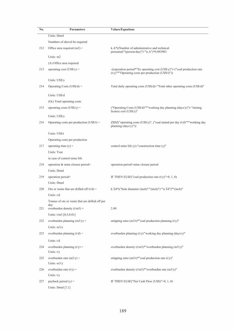
189
No. Parameters Values/Equations
Units: Dmnl
Numbers of shovel be required
212 Office area required (m2) = k.A*((Number of administrative and technical personnel/"(person/day)")^"n.A")*0.092903
Units: m2
(A) Office area required
213 operating cost (US$/y) = -((operation period*"fix operating cost (US$/y)")+("coal production rate (t/y)"*"Operating costs per production (US$/t)"))
Units: US$/y
214 Operating Costs (US$/d) = Total daily operating costs (US$/d)+"Total other operating costs (US$/d)"
Units: US$/d
(Oc) Total operating costs
215 operating costs (US$/y) = ("Operating Costs (US$/d)"*"working day planning (days/y)")+"mining licence cost (US$/y)"
Units: US$/y
216 Operating costs per production (US$/t) = ZIDZ("operating costs (US$/y)", ("coal mined per day (t/d)"*"working day planning (days/y)"))
Units: US$/t
Operating costs per production
217 operating time (y) = control mine life (y)-"construction time (y)"
Units: Year
in case of control mine life
218 operation & mine closure period= operation period+mine closure period
Units: Dmnl
219 operation period= IF THEN ELSE("coal production rate (t/y)">0, 1, 0)
Units: Dmnl
220 Ore or waste that are drilled off (t/d) = k.Td*(("hole diameter (inch)"/"(inch)")^"n.Td")*"(inch)"
Units: t/d
Tonnes of ore or waste that are drilled off per day
221 overburden density (t/m3) = 2.40
Units: t/m3 [0,5,0.01]
222 overburden planning (m3/y) = stripping ratio (m3/t)*"coal production planning (t/y)"
Units: m3/y
223 overburden planning (t/d) = overburden planning (t/y)/"working day planning (days/y)"
Units: t/d
224 overburden planning (t/y) = overburden density (t/m3)*"overburden planning (m3/y)" Units: t/y
225 overburden rate (m3/y) = stripping ratio (m3/t)*"coal production rate (t/y)"
Units: m3/y
226 overburden rate (t/y) = overburden density (t/m3)*"overburden rate (m3/y)"
Units: t/y
227 payback period (y) = IF THEN ELSE("Net Cash Flow (US$)">0, 1, 0)
Units: Dmnl [?,1]
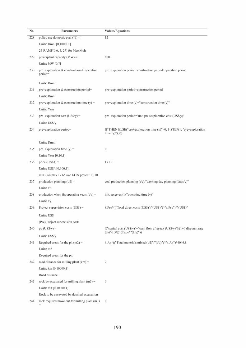
190
No. Parameters Values/Equations
228 policy use domestic coal (%) = 12
Units: Dmnl [0,100,0.1]
25-RAMP(0.6, 5, 27) for Mae Moh
229 powerplant capacity (MW) = 800
Units: MW [0,?]
230 pre+exploration & construction & operation period=
pre+exploration period+construction period+operation period
Units: Dmnl
231 pre+exploration & construction period= pre+exploration period+construction period
Units: Dmnl
232 pre+exploration & construction time (y) = pre+exploration time (y)+"construction time (y)"
Units: Year
233 pre+exploration cost (US$/y) = pre+exploration period*"unit pre+exploration cost (US$/y)"
Units: US$/y
234 pre+exploration period= IF THEN ELSE("pre+exploration time (y)">0, 1-STEP(1, "pre+exploration time (y)"), 0)
Units: Dmnl
235 pre+exploration time (y) = 0
Units: Year [0,10,1]
236 price (US$/t) = 17.10
Units: US$/t [0,100,1]
min 7.64 max 17.65 ave 14.09 present 17.10
237 production planning (t/d) = coal production planning (t/y)/"working day planning (days/y)"
Units: t/d
238 production when fix operating years (t/y) = init. reserves (t)/"operating time (y)"
Units: t/y
239 Project supervision costs (US$) = k.Psc*(("Total direct costs (US$)"/"(US$)")^"n.Psc")*"(US$)"
Units: US$
(Psc) Project supervision costs
240 pv (US$/y) = (("capital cost (US$/y)"+"cash flow after-tax (US$/y)")/(1+("discount rate (%)"/100))^(Time*"(1/y)"))
Units: US$/y
241 Required areas for the pit (m2) = k.Ap*(("Total materials mined (t/d)"/"(t/d)")^"n.Ap")*4046.8
Units: m2
Required areas for the pit
242 road distance for milling plant (km) = 2
Units: km [0,10000,1]
Road distance
243 rock be excavated for milling plant (m3) = 0
Units: m3 [0,10000,1]
Rock to be excavated by detailed excavation
244 rock required move out for milling plant (m3) =
0
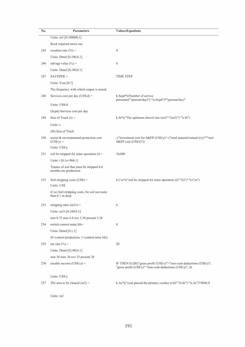
191
No. Parameters Values/Equations
Units: m3 [0,100000,1]
Rock required move out
245 royalties rate (%) = 4
Units: Dmnl [0,100,0.1]
246 salvage value (%) = 0
Units: Dmnl [0,100,0.1]
247 SAVEPER = TIME STEP
Units: Year [0,?]
The frequency with which output is stored.
248 Services cost per day (US$/d) = k.Scpd*((Number of service personnel/"(person/day)")^"n.Scpd")*"(person/day)"
Units: US$/d
(Scpd) Services cost per day
249 Size of Truck (t) = k.St*(("The optimum shovel size (m3)"/"(m3)")^"n.St")
Units: t
(St) Size of Truck
250 social & environmental protection cost (US$/y) =
-("investment cost for S&EP (US$/y)"+("total material mined (t/y)"*"unit S&EP cost (US$/t)"))
Units: US$/y
251 soil be stripped for mine operation (t) = 10,000
Units: t [0,1e+006,1]
Tonnes of soil that must be stripped 4-6 months ore production
252 Soil stripping costs (US$) = k.Css*(("soil be stripped for mine operation (t)"/"(t)")^"n.Css")
Units: US$
(Css) Soil stripping costs, for soil not more than 6.1 m deep
253 stripping ratio (m3/t) = 6
Units: m3/t [0,100,0.1]
min 0.75 max 6.0 ave 3.38 present 3.38
254 switch control mine life= 0
Units: Dmnl [0,1,1]
(0=control production, 1=control mine life)
255 tax rate (%) = 20
Units: Dmnl [0,100,0.1]
min 20 max 30 ave 25 present 20
256 taxable income (US$/y)) = IF THEN ELSE("gross profit (US$/y)">"non-cash deductions (US$/y)", "gross profit (US$/y)"-"non-cash deductions (US$/y)", 0)
Units: US$/y
257 The area to be cleared (m2) = k.Ac*(("coal passed the primary crusher (t/d)"/"(t/d)")^"n.Ac")*4046.8
Units: m2

192
No. Parameters Values/Equations
The area to be cleared for concentrator building, crusher building, etc.
258 The optimum shovel size (m3) = k.S*(("Total materials mined (t/d)"/"(t/d)")^"n.S")*0.764554
Units: m3
(S) The optimum shovel size of norminal dipper capacity
259 TIME STEP = 1
Units: Year [0,10,0.1]
The time step for the simulation.
260 Total clearing cost (US$) = k.Cc*(("Required areas for the pit (m2)"/"(m2)")^"n.Cc")
Units: US$
(Cc) Total clearing cost
261 Total concentrator operating costs (US$/d) = Crushing costs per day (US$/d)
Units: US$/d
Total concentrator operating costs
262 Total costs per production (US$/t) = ZIDZ("Total Mining Cost Estimation (US$/y)", "coal production planning (t/y)")
Units: US$/t
Total costs per production
263 Total daily operating costs (US$/d) = Total concentrator operating costs (US$/d)+"Total pit operation costs (US$/d)"
Units: US$/d
Total daily operating costs
264 Total direct costs (US$) = Total general plan capital costs (US$)+"Total mine associated capital costs (US$)"+"Total mine equipment costs (US$)"+"Total mill associated capital costs (US$)"
Total pit services cost (US$)
Units: US$
(D) Total direct costs
265 Total general plan capital costs (US$) = Changehouse cost (US$)+"Cost of office (US$)"+"Cost of maintenance shop (US$)"
Units: US$
Total general plan capital costs
266 total material mined (t/y) = coal production rate (t/y)+"overburden rate (t/y)"
Units: t/y
267 Total materials mined (t/d) = coal mined per day (t/d)+"Waste mined per day (t/d)"
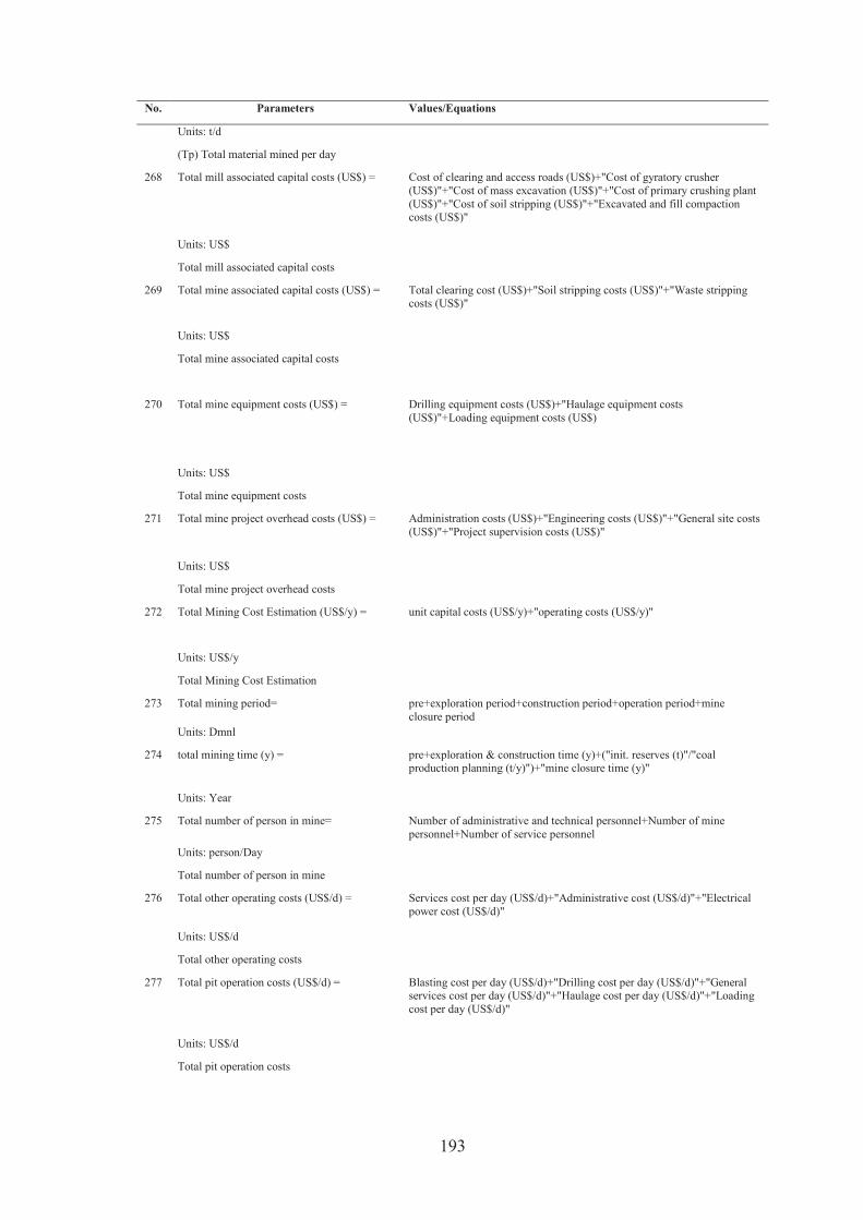
193
No. Parameters Values/Equations
Units: t/d
(Tp) Total material mined per day
268 Total mill associated capital costs (US$) = Cost of clearing and access roads (US$)+"Cost of gyratory crusher (US$)"+"Cost of mass excavation (US$)"+"Cost of primary crushing plant (US$)"+"Cost of soil stripping (US$)"+"Excavated and fill compaction costs (US$)"
Units: US$
Total mill associated capital costs
269 Total mine associated capital costs (US$) = Total clearing cost (US$)+"Soil stripping costs (US$)"+"Waste stripping costs (US$)"
Units: US$
Total mine associated capital costs
270 Total mine equipment costs (US$) = Drilling equipment costs (US$)+"Haulage equipment costs (US$)"+Loading equipment costs (US$)
Units: US$
Total mine equipment costs
271 Total mine project overhead costs (US$) = Administration costs (US$)+"Engineering costs (US$)"+"General site costs (US$)"+"Project supervision costs (US$)"
Units: US$
Total mine project overhead costs
272 Total Mining Cost Estimation (US$/y) = unit capital costs (US$/y)+"operating costs (US$/y)"
Units: US$/y
Total Mining Cost Estimation
273 Total mining period= pre+exploration period+construction period+operation period+mine closure period
Units: Dmnl
274 total mining time (y) = pre+exploration & construction time (y)+("init. reserves (t)"/"coal production planning (t/y)")+"mine closure time (y)"
Units: Year
275 Total number of person in mine= Number of administrative and technical personnel+Number of mine personnel+Number of service personnel
Units: person/Day
Total number of person in mine
276 Total other operating costs (US$/d) = Services cost per day (US$/d)+"Administrative cost (US$/d)"+"Electrical power cost (US$/d)"
Units: US$/d
Total other operating costs
277 Total pit operation costs (US$/d) = Blasting cost per day (US$/d)+"Drilling cost per day (US$/d)"+"General services cost per day (US$/d)"+"Haulage cost per day (US$/d)"+"Loading cost per day (US$/d)"
Units: US$/d
Total pit operation costs
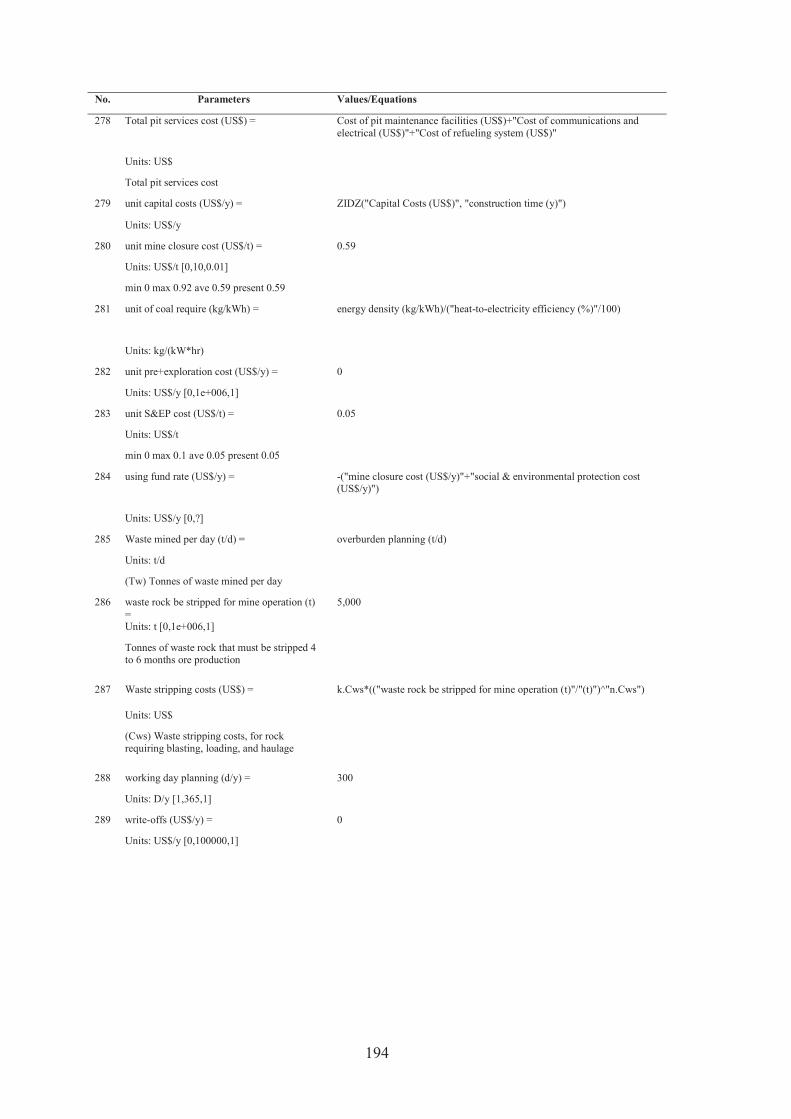
194
No. Parameters Values/Equations
278 Total pit services cost (US$) = Cost of pit maintenance facilities (US$)+"Cost of communications and electrical (US$)"+"Cost of refueling system (US$)"
Units: US$
Total pit services cost
279 unit capital costs (US$/y) = ZIDZ("Capital Costs (US$)", "construction time (y)")
Units: US$/y
280 unit mine closure cost (US$/t) = 0.59
Units: US$/t [0,10,0.01]
min 0 max 0.92 ave 0.59 present 0.59
281 unit of coal require (kg/kWh) = energy density (kg/kWh)/("heat-to-electricity efficiency (%)"/100)
Units: kg/(kW*hr)
282 unit pre+exploration cost (US$/y) = 0
Units: US$/y [0,1e+006,1]
283 unit S&EP cost (US$/t) = 0.05
Units: US$/t
min 0 max 0.1 ave 0.05 present 0.05
284 using fund rate (US$/y) = -("mine closure cost (US$/y)"+"social & environmental protection cost (US$/y)")
Units: US$/y [0,?]
285 Waste mined per day (t/d) = overburden planning (t/d)
Units: t/d
(Tw) Tonnes of waste mined per day
286 waste rock be stripped for mine operation (t) =
5,000
Units: t [0,1e+006,1]
Tonnes of waste rock that must be stripped 4 to 6 months ore production
287 Waste stripping costs (US$) = k.Cws*(("waste rock be stripped for mine operation (t)"/"(t)")^"n.Cws")
Units: US$
(Cws) Waste stripping costs, for rock requiring blasting, loading, and haulage
288 working day planning (d/y) = 300
Units: D/y [1,365,1]
289 write-offs (US$/y) = 0
Units: US$/y [0,100000,1]
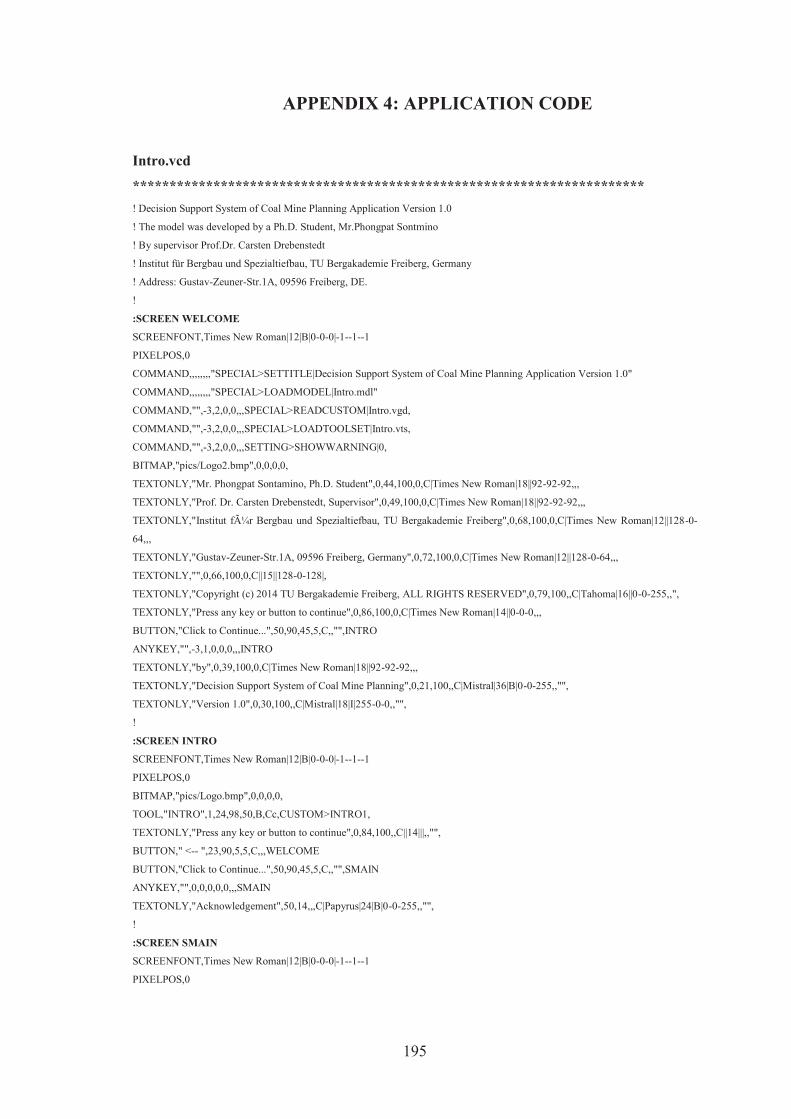
195
IV. APPENDIX 4: APPLICATION CODE
Intro.vcd
********************************************************************** ! Decision Support System of Coal Mine Planning Application Version 1.0
! The model was developed by a Ph.D. Student, Mr.Phongpat Sontmino
! By supervisor Prof.Dr. Carsten Drebenstedt
! Institut für Bergbau und Spezialtiefbau, TU Bergakademie Freiberg, Germany
! Address: Gustav-Zeuner-Str.1A, 09596 Freiberg, DE.
!
:SCREEN WELCOME
SCREENFONT,Times New Roman|12|B|0-0-0|-1--1--1
PIXELPOS,0
COMMAND,,,,,,,,"SPECIAL>SETTITLE|Decision Support System of Coal Mine Planning Application Version 1.0"
COMMAND,,,,,,,,"SPECIAL>LOADMODEL|Intro.mdl"
COMMAND,"",-3,2,0,0,,,SPECIAL>READCUSTOM|Intro.vgd,
COMMAND,"",-3,2,0,0,,,SPECIAL>LOADTOOLSET|Intro.vts,
COMMAND,"",-3,2,0,0,,,SETTING>SHOWWARNING|0,
BITMAP,"pics/Logo2.bmp",0,0,0,0,
TEXTONLY,"Mr. Phongpat Sontamino, Ph.D. Student",0,44,100,0,C|Times New Roman|18||92-92-92,,,
TEXTONLY,"Prof. Dr. Carsten Drebenstedt, Supervisor",0,49,100,0,C|Times New Roman|18||92-92-92,,,
TEXTONLY,"Institut für Bergbau und Spezialtiefbau, TU Bergakademie Freiberg",0,68,100,0,C|Times New Roman|12||128-0-
64,,,
TEXTONLY,"Gustav-Zeuner-Str.1A, 09596 Freiberg, Germany",0,72,100,0,C|Times New Roman|12||128-0-64,,,
TEXTONLY,"",0,66,100,0,C||15||128-0-128|,
TEXTONLY,"Copyright (c) 2014 TU Bergakademie Freiberg, ALL RIGHTS RESERVED",0,79,100,,C|Tahoma|16||0-0-255,,",
TEXTONLY,"Press any key or button to continue",0,86,100,0,C|Times New Roman|14||0-0-0,,,
BUTTON,"Click to Continue...",50,90,45,5,C,,"",INTRO
ANYKEY,"",-3,1,0,0,0,,,INTRO
TEXTONLY,"by",0,39,100,0,C|Times New Roman|18||92-92-92,,,
TEXTONLY,"Decision Support System of Coal Mine Planning",0,21,100,,C|Mistral|36|B|0-0-255,,"",
TEXTONLY,"Version 1.0",0,30,100,,C|Mistral|18|I|255-0-0,,"",
!
:SCREEN INTRO
SCREENFONT,Times New Roman|12|B|0-0-0|-1--1--1
PIXELPOS,0
BITMAP,"pics/Logo.bmp",0,0,0,0,
TOOL,"INTRO",1,24,98,50,B,Cc,CUSTOM>INTRO1,
TEXTONLY,"Press any key or button to continue",0,84,100,,C||14|||,,"",
BUTTON," <-- ",23,90,5,5,C,,,WELCOME
BUTTON,"Click to Continue...",50,90,45,5,C,,"",SMAIN
ANYKEY,"",0,0,0,0,0,,,SMAIN
TEXTONLY,"Acknowledgement",50,14,,,C|Papyrus|24|B|0-0-255,,"",
!
:SCREEN SMAIN
SCREENFONT,Times New Roman|12|B|0-0-0|-1--1--1
PIXELPOS,0
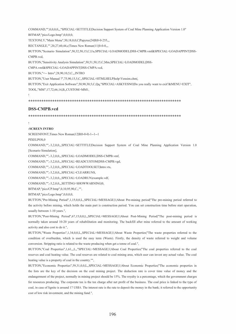
196
COMMAND,"",0,0,0,0,,,"SPECIAL>SETTITLE|Decision Support System of Coal Mine Planning Application Version 1.0"
BITMAP,"pics/Logo.bmp",0,0,0,0,
TEXTONLY,"Main Menu",50,18,0,0,C|Papyrus|24|B|0-0-255,,,
RECTANGLE,"",20,27,60,44,c|Times New Roman|11||0-0-0,,,
BUTTON,"Scenario Simulation",50,32,50,15,C,Uu,SPECIAL>LOADMODEL|DSS-CMPB.vmf&SPECIAL>LOADAPPINT|DSS-
CMPB.vcd,
BUTTON,"Sensitivity Analysis Simulation",50,51,50,15,C,Mm,SPECIAL>LOADMODEL|DSS-
CMPA.vmf&SPECIAL>LOADAPPINT|DSS-CMPA.vcd,
BUTTON,"<-- Intro",28,90,10,5,C,,,INTRO
BUTTON,"User Manual ?",75,90,15,5,C,,SPECIAL>HTMLHELP|help\Vensim.chm|,
BUTTON,"Exit Application Software",50,90,30,5,C,Qq,"SPECIAL>ASKYESNO|Do you really want to exit?&MENU>EXIT",
TOOL,"MM",17,72,66,14,B,,CUSTOM>MM1,
!
**********************************************************************
DSS-CMPB.vcd
********************************************************************** !
:SCREEN INTRO
SCREENFONT,Times New Roman|12|B|0-0-0|-1--1--1
PIXELPOS,0
COMMAND,"",-3,2,0,0,,,SPECIAL>SETTITLE|Decision Support System of Coal Mine Planning Application Version 1.0
[Scenario Simulation],
COMMAND,"",-3,2,0,0,,,SPECIAL>LOADMODEL|DSS-CMPB.vmf,
COMMAND,"",-3,2,0,0,,,SPECIAL>READCUSTOM|DSS-CMPB.vgd,
COMMAND,"",-3,2,0,0,,,SPECIAL>LOADTOOLSET|Intro.vts,
COMMAND,"",-3,2,0,0,,,SPECIAL>CLEARRUNS,
COMMAND,"",-3,2,0,0,,,SPECIAL>LOADRUN|example.vdf,
COMMAND,"",-3,2,0,0,,,SETTING>SHOWWARNING|0,
BITMAP,"pics/CP.bmp",0,10,95,90,C,,"",
BITMAP,"pics/Logo.bmp",0,0,0,0,
BUTTON,"Pre-Mining Period",1,15,0,0,L,,SPECIAL>MESSAGE|1|About Pre-mining period|"The pre-mining period referred to
the activity before mining, which holds the main part is construction period. You can set construction time before start operation,
usually between 1-10 years.",
BUTTON,"Post-Mining Period",67,15,0,0,L,,SPECIAL>MESSAGE|1|About Post-Mining Period|"The post-mining period is
normally taken around 10-20 years of rehabilitation and monitoring. The backfill after mine referred to the amount of working
activity and also cost to do it.",
BUTTON,"Waste Properties",1,34,0,0,L,,SPECIAL>MESSAGE|1|About Waste Properties|"The waste properties referred to the
condition of overburden, which is used the easy term (Waste). Firstly, the density of waste referred to weight and volume
conversion. Stripping ratio is related to the waste producing when get a tonne of coal.",
BUTTON,"Coal Properties",1,61,,,L,,"SPECIAL>MESSAGE|1|About Coal Properties|"The coal properties referred to the coal
reserves and coal heating value. The coal reserves are related to coal mining area, which user can invest any actual value. The coal
heating value is a property of coal in the country."",
BUTTON,"Economic Properties",59,31,0,0,L,,SPECIAL>MESSAGE|1|About Economic Properties|"The economic properties in
the lists are the key of the decision on the coal mining project. The deduction rate is cover time value of money and the
endangerment of the project, normally in mining project should be 15%. The royalty is a percentage, which the government charges
for resources producing. The corporate tax is the tax charge after net profit of the business. The coal price is linked to the type of
coal, in case of lignite is around 17 US$/t. The interest rate is the rate to deposit the money in the bank; it referred to the opportunity
cost of low risk investment, and the mining fund.",

197
BUTTON,"SIMULATE",83,94,,5,,,"SIMULATE>RUNNAME|?Please put the name for new
scenario&MENU>RUN1|O",RESULT1
MODVAR,"\"init. reserves (t)\"",18,65,8,0,,,Caol reserves,
TEXTONLY,"Coal reserves",1,65,0,0,,,,
TEXTONLY,"t",26,65,0,0,,,,
MODVAR,"\"coal heating value (kcal/kg)\"",18,69,8,0,,,,
TEXTONLY,"Coal heating value",1,69,0,0,,,,
TEXTONLY,"kcal/kg",26,69,0,0,,,,
MODVAR,"\"construction time (y)\"",16,19,5,0,,,Caol reserves,
TEXTONLY,"Construction times",1,19,0,0,,,,
TEXTONLY,"years",21,19,0,0,,,,
MODVAR,"\"overburden density (t/m3)\"",13,38,10,0,,,,
TEXTONLY,"Waste density",1,38,0,0,,,,
TEXTONLY,"t/m3",23,38,0,0,,,,
MODVAR,"\"royalties rate (%)\"",71,39,10,0,,,,
TEXTONLY,"Royalties",59,39,0,0,,,,
TEXTONLY,"%",81,39,0,0,,,,
MODVAR,"\"mine closure time (y)\"",83,19,5,0,,,,
TEXTONLY,"Mine closure times",67,19,0,0,,,,
TEXTONLY,"years",88,19,0,0,,,,
MODVAR,"\"stripping ratio (m3/t)\"",13,42,10,0,,,,
TEXTONLY,"Stripping ratio",1,42,0,0,,,,
TEXTONLY,"m3/t",23,42,0,0,,,,
MODVAR,"\"tax rate (%)\"",71,43,10,0,,,,
TEXTONLY,"Corporate tax",59,43,0,0,,,,
TEXTONLY,"%",81,43,0,0,,,,
BUTTON,"Power Plant Properties",1,75,,,,,"SPECIAL>MESSAGE|1|About Power Plant Properties|"The power plant properties
referred to power plant capacity, which connected to the demand of coal, and it mean the size of mining (mining production rate).
Moreover, the power efficiency is the proportion of energy input to produce electricity, which is between 30-65%."",
MODVAR,"\"powerplant capacity (MW)\"",18,79,8,0,,,,
TEXTONLY,"Power plant capacity",1,79,0,0,,,,
TEXTONLY,"MW",26,79,0,0,,,,
MODVAR,"\"price (US$/t)\"",71,47,10,0,,,,
TEXTONLY,"Coal price",59,47,0,0,,,,
TEXTONLY,"US$/t",81,47,0,0,,,,
MODVAR,"\"discount rate (%)\"",71,35,10,0,,,,
TEXTONLY,"Discount rate",59,35,0,0,,,,
TEXTONLY,"%",81,35,0,0,,,,
BUTTON,"Mining Conditions",51,61,,,L,,"SPECIAL>MESSAGE|1|About Mining conditions|"The mining conditions referred to
the distance between mining site and crushing plant, which related to the cost of road building. The working day planning is linked
up to the output rate should be per day. The drill hole diameter is related to quantity of drilling machine, which defended the
production pace. Finally, the equipment life cycle related to new investment to replace the old machines."",
MODVAR,"\"road distance for milling plant (km)\"",72,65,5,0,,,Caol reserves,
TEXTONLY,"Distance to crushing plant",51,65,,,,,"",
TEXTONLY,"km",77,65,0,0,,,,
MODVAR,"\"working day planning (d/y)\"",72,69,5,0,,,Caol reserves,
TEXTONLY,"Working day planning",51,69,0,0,,,,
TEXTONLY,"d/y",77,69,0,0,,,,
MODVAR,"\"hole diameter (inch)\"",72,73,5,0,,,Caol reserves,

198
TEXTONLY,"Drill hole diameter",51,73,0,0,,,,
TEXTONLY,"inch",77,73,0,0,,,,
MODVAR,"\"soil be stripped for mine operation (t)\"",35,46,8,0,,,,
TEXTONLY,"Soil stripped for starting operation",1,46,0,0,,,,
TEXTONLY,"t",43,46,0,0,,,,
MODVAR,"\"waste rock be stripped for mine operation (t)\"",35,50,8,0,,,,
TEXTONLY,"Waste rock stripped for starting operation",1,50,0,0,,,,
TEXTONLY,"t",43,50,0,0,,,,
MODVAR,"\"backfill ratio (%)\"",83,23,5,0,,,,
TEXTONLY,"Backfill after mine",67,23,0,0,,,,
TEXTONLY,"%",88,23,0,0,,,,
BUTTON,"Mining Fund for S+EP and Mine Closure Period",28,15,0,0,L,,SPECIAL>MESSAGE|1|"About Mining Fund for\
Social & Environmental Protection and Mine Closure Period"|"The mining fund is a innovative style of mining standard, which
mining should take a responsibility of social and environmental protection, and mine closure, by spending some money to establish
a funding that used only specific purposes. You can put the suitable value in your mining area. Mining fund rate related to
production rate, Unit Social & Environmental Protection (S&EP) related to total material mine rate, and Unit Mine closure related
to overburden producing rate.",
MODVAR,"\"mining fund rate (US$/t)\"",50,19,5,0,,,,
TEXTONLY,"Mine fund rate",28,19,0,0,,,,
TEXTONLY,"US$/t",55,19,0,0,,,,
MODVAR,"\"deposit interest rate (%/y)\"",71,51,10,0,,,,
TEXTONLY,"Interest rate",59,51,0,0,,,,
TEXTONLY,"%",81,51,0,0,,,,
MODVAR,"\"unit S&EP cost (US$/t)\"",50,23,5,0,,,,
TEXTONLY,"Unit S&EP cost",28,23,0,0,,,,
TEXTONLY,"US$/t",55,23,0,0,,,,
MODVAR,"\"unit mine closure cost (US$/t)\"",50,27,5,0,,,,
TEXTONLY,"Unit mine closure cost",28,27,0,0,,,,
TEXTONLY,"US$/t",55,27,0,0,,,,
BUTTON,"Print",22,94,0,5,,,PRINT>!||,
BUTTON,"<-- Back to main
menu",10,94,19,5,C,EeXx,"SPECIAL>LOADMODEL|intro.mdl&SPECIAL>LOADAPPINT|intro.vcd@2",
MODVAR,"\"heat-to-electricity efficiency (%)\"",18,83,8,,,,"",
TEXTONLY,"Power efficiency",1,83,,,,,"",
TEXTONLY,"%",26,83,0,0,,,,
BUTTON,"Help?",28,94,,5,,,"SPECIAL>MESSAGE|1|Help|"You can change values in the box related to your coal mining site
condition. After that, click (SIMULATE) button for calculation result. The application will ask you to identify the new file name, so
you can put the name that you want or click the name in the list for overwrite it."",
TEXTONLY,"Scenario Simulation Conditions",50,4,,,C|Papyrus|20|B|0-0-255,,"",
MODVAR,"FINAL TIME",60,95,5,0,,,,
TEXTONLY,"Simulation Period",45,95,,,,,"",
TEXTONLY,"years",66,95,0,0,,,,
MODVAR,"\"equipment life cycle (Y)\"",72,77,5,,,,"",
TEXTONLY,"Equipment life cycle",51,77,,,,,"",
TEXTONLY,"years",77,77,,,,,"",
!
:SCREEN RESULT1
SCREENFONT,Times New Roman|10||0-0-0|-1--1--1
PIXELPOS,0

199
COMMAND,"",-3,2,0,0,,,SPECIAL>SETTITLE|Decision Support System of Coal Mine Planning Application Version 1.0
[Scenario Simulation],
BITMAP,"pics/CP.bmp",0,10,95,90,C,,,
BITMAP,"pics/Logo.bmp",0,0,0,0,
BUTTON,"<-- New simulation conditions",50,94,,5,C,,"",INTRO
BUTTON,"Print",1,94,0,5,,,PRINT>!||,
TEXTONLY,"Shovel bucket size (m3) =",55,40,0,0,|Times New Roman|12||0-0-0,,,
SHOWVAR,"\"The optimum shovel size (m3)\"",79,40,0,0,|Times New Roman|12|B|0-0-255,,,
TEXTONLY,"Number of shovel =",55,37,,,|Times New Roman|12||0-0-0,,"",
SHOWVAR,"Numbers of shovel be required",79,37,0,0,|Times New Roman|12|B|0-0-255,,,
TEXTONLY,"Truck size (t) =",55,46,0,0,|Times New Roman|12||0-0-0,,,
SHOWVAR,"\"Size of Truck (t)\"",79,46,0,0,|Times New Roman|12|B|0-0-255,,,
TEXTONLY,"Number of truck =",55,43,,,|Times New Roman|12||0-0-0,,"",
SHOWVAR,"Number of Truck Required",79,43,0,0,|Times New Roman|12|B|0-0-255,,,
TEXTONLY,"Capital cost (US$) =",8,16,0,0,|Times New Roman|12||0-0-0,,,
SHOWVAR,"\"Capital Costs (US$)\"",29,16,0,0,|Times New Roman|12|B|0-0-255,,,
TEXTONLY,"Operating cost (US$/d) =",8,19,0,0,|Times New Roman|12||0-0-0,,,
SHOWVAR,"\"Operating Costs (US$/d)\"",29,19,0,0,|Times New Roman|12|B|0-0-255,,,
TEXTONLY,"Cost Estimation",8,13,0,0,|Times New Roman|12|BI|0-0-0,,,
TEXTONLY,"Equipment Estimation",55,31,0,0,|Times New Roman|12|BI|0-0-0,,,
TEXTONLY,"Coal production rate (t/y) =",44,22,0,0,|Times New Roman|12||0-0-0,,,
SHOWVAR,"\"coal production planning (t/y)\"",71,22,0,0,|Times New Roman|12|B|0-0-255,,,
TEXTONLY,"Waste producing rate (m3/y) =",44,25,0,0,|Times New Roman|12||0-0-0,,,
SHOWVAR,"\"overburden planning (m3/y)\"",71,25,0,0,|Times New Roman|12|B|0-0-255,,,
TEXTONLY,"Mining Condition",44,19,0,0,|Times New Roman|12|BI|0-0-0,,,
TEXTONLY,"This coal mining project should be:",50,11,0,0,C|Times New Roman|16|B|0-0-0,,,
SHOWVAR,"Accept or Reject?0=Reject_Project?1=Accept_Project",71,11,0,0,|Times New Roman|16|BI|255-0-0,,,
TEXTONLY,"Because of, the NPV Balance is (US$)",44,15,0,0,|Times New Roman|12||0-0-0,,,
SHOWVAR,"NPV Balance",71,15,0,0,|Times New Roman|12|B|0-0-255,,,
TEXTONLY,"Number of drilling equipment =",55,34,,,|Times New Roman|12||0-0-0,,"",
SHOWVAR,"Numbers of drilling machine",79,34,0,0,|Times New Roman|12|B|0-0-255,,,
TEXTONLY,"Service personnel =",4,45,0,0,|Times New Roman|12||0-0-0,,,
SHOWVAR,"Number of service personnel",34,45,0,0,|Times New Roman|12|B|0-0-255,,,
TEXTONLY,"Mine personnel =",4,42,0,0,|Times New Roman|12||0-0-0,,,
SHOWVAR,"Number of mine personnel",34,42,0,0,|Times New Roman|12|B|0-0-255,,,
TEXTONLY,"Worker Estimation",4,36,0,0,|Times New Roman|12|BI|0-0-0,,,
TEXTONLY,"Administrative and technical personnel =",4,39,0,0,|Times New Roman|12||0-0-0,,,
SHOWVAR,"Number of administrative and technical personnel",34,39,0,0,|Times New Roman|12|B|0-0-255,,,
TEXTONLY,"Unit of coal required (kg/kWh) =",48,75,0,0,|Times New Roman|12||0-0-0,,,
SHOWVAR,"\"unit of coal require (kg/kWh)\"",78,75,0,0,|Times New Roman|12|B|0-0-255,,,
TEXTONLY,"Electricity production rate (GWh/y) =",48,72,0,0,|Times New Roman|12||0-0-0,,,
SHOWVAR,"\"electricity production rate (GWh/y)\"",78,72,0,0,|Times New Roman|12|B|0-0-255,,,
TEXTONLY,"Power Plant Information",48,66,0,0,|Times New Roman|12|BI|0-0-0,,,
TEXTONLY,"Power plant capacity (MW) =",48,69,0,0,|Times New Roman|12||0-0-0,,,
SHOWVAR,"\"powerplant capacity (MW)\"",78,69,0,0,|Times New Roman|12|B|0-0-255,,,
BUTTON,"Open data",8,94,0,5,,,MENU>LOAD_RUN|,
TEXTONLY,"Net Cash Balance (US$) =",4,75,,,|Times New Roman|12||0-0-0,,"",
SHOWVAR,"Net Cash Balance",23,75,0,0,|Times New Roman|12|B|0-0-255,,,
TEXTONLY,"Mining fund (US$) =",4,72,,,|Times New Roman|12||0-0-0,,"",
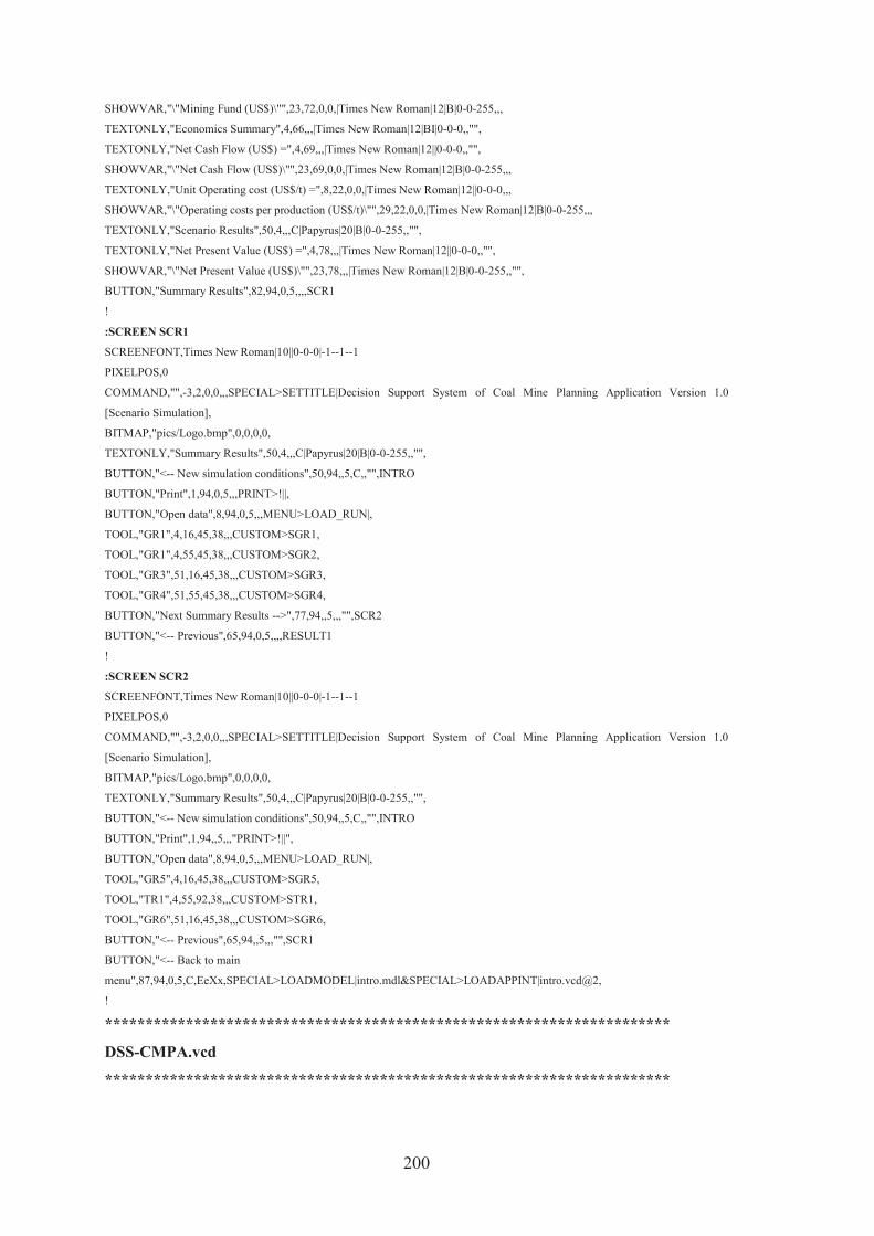
200
SHOWVAR,"\"Mining Fund (US$)\"",23,72,0,0,|Times New Roman|12|B|0-0-255,,,
TEXTONLY,"Economics Summary",4,66,,,|Times New Roman|12|BI|0-0-0,,"",
TEXTONLY,"Net Cash Flow (US$) =",4,69,,,|Times New Roman|12||0-0-0,,"",
SHOWVAR,"\"Net Cash Flow (US$)\"",23,69,0,0,|Times New Roman|12|B|0-0-255,,,
TEXTONLY,"Unit Operating cost (US$/t) =",8,22,0,0,|Times New Roman|12||0-0-0,,,
SHOWVAR,"\"Operating costs per production (US$/t)\"",29,22,0,0,|Times New Roman|12|B|0-0-255,,,
TEXTONLY,"Scenario Results",50,4,,,C|Papyrus|20|B|0-0-255,,"",
TEXTONLY,"Net Present Value (US$) =",4,78,,,|Times New Roman|12||0-0-0,,"",
SHOWVAR,"\"Net Present Value (US$)\"",23,78,,,|Times New Roman|12|B|0-0-255,,"",
BUTTON,"Summary Results",82,94,0,5,,,,SCR1
!
:SCREEN SCR1
SCREENFONT,Times New Roman|10||0-0-0|-1--1--1
PIXELPOS,0
COMMAND,"",-3,2,0,0,,,SPECIAL>SETTITLE|Decision Support System of Coal Mine Planning Application Version 1.0
[Scenario Simulation],
BITMAP,"pics/Logo.bmp",0,0,0,0,
TEXTONLY,"Summary Results",50,4,,,C|Papyrus|20|B|0-0-255,,"",
BUTTON,"<-- New simulation conditions",50,94,,5,C,,"",INTRO
BUTTON,"Print",1,94,0,5,,,PRINT>!||,
BUTTON,"Open data",8,94,0,5,,,MENU>LOAD_RUN|,
TOOL,"GR1",4,16,45,38,,,CUSTOM>SGR1,
TOOL,"GR1",4,55,45,38,,,CUSTOM>SGR2,
TOOL,"GR3",51,16,45,38,,,CUSTOM>SGR3,
TOOL,"GR4",51,55,45,38,,,CUSTOM>SGR4,
BUTTON,"Next Summary Results -->",77,94,,5,,,"",SCR2
BUTTON,"<-- Previous",65,94,0,5,,,,RESULT1
!
:SCREEN SCR2
SCREENFONT,Times New Roman|10||0-0-0|-1--1--1
PIXELPOS,0
COMMAND,"",-3,2,0,0,,,SPECIAL>SETTITLE|Decision Support System of Coal Mine Planning Application Version 1.0
[Scenario Simulation],
BITMAP,"pics/Logo.bmp",0,0,0,0,
TEXTONLY,"Summary Results",50,4,,,C|Papyrus|20|B|0-0-255,,"",
BUTTON,"<-- New simulation conditions",50,94,,5,C,,"",INTRO
BUTTON,"Print",1,94,,5,,,"PRINT>!||",
BUTTON,"Open data",8,94,0,5,,,MENU>LOAD_RUN|,
TOOL,"GR5",4,16,45,38,,,CUSTOM>SGR5,
TOOL,"TR1",4,55,92,38,,,CUSTOM>STR1,
TOOL,"GR6",51,16,45,38,,,CUSTOM>SGR6,
BUTTON,"<-- Previous",65,94,,5,,,"",SCR1
BUTTON,"<-- Back to main
menu",87,94,0,5,C,EeXx,SPECIAL>LOADMODEL|intro.mdl&SPECIAL>LOADAPPINT|intro.vcd@2,
!
**********************************************************************
DSS-CMPA.vcd
**********************************************************************

201
!
:SCREEN INTRO
SCREENFONT,Times New Roman|12|B|0-0-0|-1--1--1
PIXELPOS,0
COMMAND,,,,,,,,"SPECIAL>SETTITLE|Decision Support System of Coal Mine Planning Application Version 1.0 [Sensitivity
Analysis]"
COMMAND,,,,,,,,"SPECIAL>LOADMODEL|DSS-CMPA.vmf"
COMMAND,,,,,,,,"SPECIAL>READCUSTOM|DSS-CMPA.vgd"
COMMAND,"",-3,2,0,0,,,SPECIAL>LOADTOOLSET|DSS-CMPA.vts,
COMMAND,"",-3,2,0,0,,,SPECIAL>CLEARRUNS,
COMMAND,"",-3,2,0,0,,,SPECIAL>LOADRUN|example.vdf,
COMMAND,"",-3,2,0,0,,,SETTING>SHOWWARNING|0,
BITMAP,"pics/CP.bmp",0,10,95,90,C,,,
BITMAP,"pics/Logo.bmp",0,0,0,0,
BUTTON,"Pre-Mining Period",1,16,0,0,L,,SPECIAL>MESSAGE|1|About Pre-mining period|"The pre-mining period referred to
the activity before mining, which holds the main part is the construction period. "",
BUTTON,"Post-Mining Period",67,16,0,0,L,,SPECIAL>MESSAGE|1|About Post-Mining Period|"The post-mining period is
normally taken around 10-20 years of rehabilitation and monitoring. The backfill after mine referred to the amount of working
activity and also cost to do it.",
BUTTON,"Waste properties",1,35,0,0,L,,SPECIAL>MESSAGE|1|About Waste Properties|"The waste properties referred to the
condition of overburden, which is used
BUTTON,"Coal properties",1,61,,,L,,"SPECIAL>MESSAGE|1|About Coal Properties|"The coal properties referred to the coal
reserves and coal heating value. The coal reserves are related to coal mining area, which user can invest any actual value. The coal
heating value is a property of coal in the country."",
BUTTON,"Economic properties",59,32,0,0,L,,SPECIAL>MESSAGE|1|About Economic Properties|"The economic properties in
the lists are the key of the decision on the coal mining project. The deduction rate is cover time value of money and the
endangerment of the project, normally in mining
BUTTON,"RUN
SENSITIVITY",83,94,,5,,,"SPECIAL>CLEARRUNS|&SIMULATE>RUNNAME|Sensitivity&SIMULATE>SENSITIVITY|Sensi.
vsc&SIMULATE>SENSSAVELIST|Sensi_Result.lst&MENU>RUN_SENSITIVITY|O",RESULT_SA1
MODVAR,"IR MAX",23,65,5,,,,"Caol reserves",
TEXTONLY,"Coal reserves",1,65,0,0,,,,
TEXTONLY,"t",28,65,0,0,,,,
MODVAR,"CHV MAX",23,69,5,,,,"",
TEXTONLY,"Coal heating value",1,69,0,0,,,,
TEXTONLY,"kcal/kg",28,69,0,0,,,,
MODVAR,"CT MAX",19,20,3,0,,,Caol reserves,
TEXTONLY,"Construction times",1,20,0,0,,,,
TEXTONLY,"years",22,20,0,0,,,,
MODVAR,"OD MAX",20,39,5,0,,,,
TEXTONLY,"Waste density",1,39,0,0,,,,
TEXTONLY,"t/m3",25,39,0,0,,,,
MODVAR,"RR MAX",77,40,5,0,,,,
TEXTONLY,"Royalties",59,40,0,0,,,,
TEXTONLY,"%",82,40,0,0,,,,
MODVAR,"MCT MAX",86,20,3,0,,,,
TEXTONLY,"Mine closure times",67,20,0,0,,,,
TEXTONLY,"years",89,20,0,0,,,,
MODVAR,"SR MAX",20,43,5,0,,,,

202
TEXTONLY,"Stripping ratio",1,43,0,0,,,,
TEXTONLY,"m3/t",25,43,0,0,,,,
MODVAR,"TR MAX",77,44,5,0,,,,
TEXTONLY,"Corporate tax",59,44,0,0,,,,
TEXTONLY,"%",82,44,0,0,,,,
BUTTON,"Power Plant Properties",1,76,0,0,,,SPECIAL>MESSAGE|1|About Power Plant Properties|"The power plant properties
referred to power plant capacity, which connected to the demand of coal, and it mean the size of mining (mining production rate).
Moreover, the power efficiency is the proportion of energy input to produce electricity, which is between 30-65%.",
MODVAR,"PPC MAX",24,80,5,0,,,,
TEXTONLY,"Power plant capacity",1,80,0,0,,,,
TEXTONLY,"MW",29,80,0,0,,,,
MODVAR,"P MAX",77,48,5,0,,,,
TEXTONLY,"Coal price",59,48,0,0,,,,
TEXTONLY,"US$/t",82,48,0,0,,,,
MODVAR,"DR MAX",77,36,5,0,,,,
TEXTONLY,"Discount rate",59,36,0,0,,,,
TEXTONLY,"%",82,36,0,0,,,,
BUTTON,"Mining Conditions",51,61,,,L,,"SPECIAL>MESSAGE|1|About Mining Conditions|"The mining conditions referred to
the distance between mining site and crushing plant, which related to the cost of road building. The working day planning is linked
up to the output rate should be per day. Lastly, the drill hole diameter is related to quantity of drilling machine, which defended the
production pace."",
MODVAR,"RD MAX",76,65,4,,,,"Caol reserves",
TEXTONLY,"Distance to crushing plant",51,65,,,,,"",
TEXTONLY,"km",80,65,0,0,,,,
MODVAR,"WDP MAX",76,69,4,,,,"Caol reserves",
TEXTONLY,"Working day planning",51,69,0,0,,,,
TEXTONLY,"d/y",80,69,0,0,,,,
MODVAR,"HD MAX",76,73,4,,,,"Caol reserves",
TEXTONLY,"Drill hole diameter",51,73,0,0,,,,
TEXTONLY,"inches",80,73,,,,,"",
MODVAR,"SSO MAX",42,47,6,0,,,,
TEXTONLY,"Soil stripped for starting operation",1,47,0,0,,,,
TEXTONLY,"t",48,47,0,0,,,,
MODVAR,"WSO MAX",42,51,6,0,,,,
TEXTONLY,"Waste rock stripped for starting operation",1,51,0,0,,,,
TEXTONLY,"t",48,51,0,0,,,,
MODVAR,"BFR MAX",86,24,3,0,,,,
TEXTONLY,"Backfill after mine",67,24,0,0,,,,
TEXTONLY,"%",89,24,0,0,,,,
BUTTON,"Mining Fund for S+EP and Mine Closure Period",28,16,0,0,L,,SPECIAL>MESSAGE|1|"About Mining Fund for Social
& Environmental Protection and Mine Closure Period"|"The mining fund is a innovative style of mining standard, which mining
should spend some money for protecting the environment. "",
MODVAR,"MF MAX",51,20,4,0,,,,
TEXTONLY,"Mine fund rate",28,20,0,0,,,,
TEXTONLY,"US$/t",55,20,0,0,,,,
MODVAR,"DIR MAX",77,52,5,0,,,,
TEXTONLY,"Interest rate",59,52,0,0,,,,
TEXTONLY,"%",82,52,0,0,,,,
MODVAR,"USEP MAX",51,24,4,0,,,,

203
TEXTONLY,"Unit S&EP cost",28,24,0,0,,,,
TEXTONLY,"US$/t",55,24,0,0,,,,
MODVAR,"UMC MAX",51,28,4,0,,,,
TEXTONLY,"Unit mine closure cost",28,28,0,0,,,,
TEXTONLY,"US$/t",55,28,0,0,,,,
BUTTON,"Print",22,94,0,5,,,PRINT>!||,
BUTTON,"<-- Back to main
menu",10,94,19,5,C,EeXx,"SPECIAL>LOADMODEL|intro.mdl&SPECIAL>LOADAPPINT|intro.vcd@2",
MODVAR,"H2E MAX",24,84,5,0,,,,
TEXTONLY,"Power efficiency",1,84,0,0,,,,
TEXTONLY,"%",29,84,0,0,,,,
BUTTON,"Help?",28,94,,5,,,"SPECIAL>MESSAGE|1|Help|"This sensitivity analysis uses the monte carlo method to randdom
number in the range, which you can put in the box. the left-side box is a minimum value, and right-side is a maximum value. If you
don't want to put the range in any variable please put the same value in the both box. After complete setup the sensitivity analysis
conditions, click (RUN SENSITIVITY) button."",
TEXTONLY,"Sensitivity Analysis Conditions",50,4,,,C|Papyrus|20|B|0-0-255,,"",
MODVAR,"CT MIN",16,20,3,0,,,,
MODVAR,"IR MIN",18,65,5,,,,"",
MODVAR,"CHV MIN",18,69,5,,,,"",
MODVAR,"OD MIN",15,39,5,0,,,,
MODVAR,"RR MIN",72,40,5,0,,,,
MODVAR,"MCT MIN",83,20,3,0,,,,
MODVAR,"SR MIN",15,43,5,0,,,,
MODVAR,"TR MIN",72,44,5,0,,,,
MODVAR,"PPC MIN",19,80,5,0,,,,
MODVAR,"P MIN",72,48,5,0,,,,
MODVAR,"DR MIN",72,36,5,0,,,,
MODVAR,"RD MIN",72,65,4,,,,"",
MODVAR,"WDP MIN",72,69,4,,,,"",
MODVAR,"HD MIN",72,73,4,,,,"",
MODVAR,"SSO MIN",36,47,6,0,,,,
MODVAR,"WSO MIN",36,51,6,0,,,,
MODVAR,"BFR MIN",83,24,3,0,,,,
MODVAR,"MF MIN",47,20,4,0,,,,
MODVAR,"DIR MIN",72,52,5,0,,,,
MODVAR,"USEP MIN",47,24,4,0,,,,
MODVAR,"UMC MIN",47,28,4,0,,,,
MODVAR,"H2E MIN",19,84,5,0,,,,
MODVAR,"FINAL TIME",52,95,0,0,,,,
TEXTONLY,"Simulation Period",37,95,0,0,,,,
TEXTONLY,"years",60,95,0,0,,,,
!
:SCREEN RESULT_SA1
SCREENFONT,Times New Roman|10||0-0-0|-1--1--1
PIXELPOS,0
COMMAND,,,,,,,,"SPECIAL>SETTITLE|Decision Support System of Coal Mine Planning Application Version 1.0 [Sensitivity
Analysis]"
COMMAND,,,,,,,,"SPECIAL>SETWBITEM|Net Cash Balance"
BITMAP,"pics/Logo.bmp",0,0,0,0,

204
TEXTONLY,"Sensitivity Results-",50,2,,,R|Times New Roman|18|B|0-0-255,,"",
WBVAR,"",50,2,,,L|Times New Roman|18|BI|0-0-128,,"",
TOOL,"GR1",5,14,88,70,,,"WORKBENCH>Sensitivity Graph",
BUTTON,"Net Cash Flow",22,86,15,0,L,,,RESULT_SA2
BUTTON,"Mining Fund",42,86,15,0,L,,,RESULT_SA3
BUTTON,"NPV Balance",62,86,15,0,L,,,RESULT_SA4
BUTTON,"Net Present Value",82,86,15,0,L,,,RESULT_SA5
BUTTON,"Histrogram",2,91,20,0,L,,WORKBENCH>Bar Graph,
BUTTON,"Statistics",2,96,20,0,L,,WORKBENCH>Statistics,
BUTTON,"Print graph",24,91,0,0,L,,PRINT>GR1,
BUTTON,"Return to sensitivity condition setup",50,91,30,0,C,,,INTRO
BUTTON,"Coal Reserves",66,91,15,0,L,,,RESULT_SA6
BUTTON,"Production Rate",82,91,15,0,L,,,RESULT_SA7
!
:SCREEN RESULT_SA2
SCREENFONT,Times New Roman|10||0-0-0|-1--1--1
PIXELPOS,0
COMMAND,,,,,,,,"SPECIAL>SETTITLE|Decision Support System of Coal Mine Planning Application Version 1.0 [Sensitivity
Analysis]"
COMMAND,,,,,,,,"SPECIAL>SETWBITEM|"Net Cash Flow (US$)""
BITMAP,"pics/Logo.bmp",0,0,0,0,
TEXTONLY,"Sensitivity Results-",50,2,,,R|Times New Roman|18|B|0-0-255,,"",
WBVAR,"",50,2,,,L|Times New Roman|18|BI|0-0-128,,"",
TOOL,"GR1",5,14,88,70,,,"WORKBENCH>Sensitivity Graph",
BUTTON,"Net Cash Balance",3,86,15,0,L,,,RESULT_SA1
BUTTON,"Print graph",24,91,0,0,L,,PRINT>GR1,
BUTTON,"Return to sensitivity condition setup",50,91,30,0,C,,,INTRO
BUTTON,"Mining Fund",42,86,15,0,L,,,RESULT_SA3
BUTTON,"NPV Balance",62,86,15,0,L,,,RESULT_SA4
BUTTON,"Net Present Value",82,86,15,0,L,,,RESULT_SA5
BUTTON,"Histrogram",2,91,20,0,L,,WORKBENCH>Bar Graph,
BUTTON,"Coal Reserves",66,91,15,0,L,,,RESULT_SA6
BUTTON,"Production Rate",82,91,15,0,L,,,RESULT_SA7
BUTTON,"Statistics",2,96,20,0,L,,WORKBENCH>Statistics,
!
:SCREEN RESULT_SA3
SCREENFONT,Times New Roman|10||0-0-0|-1--1--1
PIXELPOS,0
COMMAND,,,,,,,,"SPECIAL>SETTITLE|Decision Support System of Coal Mine Planning Application Version 1.0 [Sensitivity
Analysis]"
COMMAND,,,,,,,,"SPECIAL>SETWBITEM|"Mining Fund (US$)""
BITMAP,"pics/Logo.bmp",0,0,0,0,
TEXTONLY,"Sensitivity Results-",50,2,,,R|Times New Roman|18|B|0-0-255,,"",
WBVAR,"",50,2,,,L|Times New Roman|18|BI|0-0-128,,"",
TOOL,"GR1",5,14,88,70,,,"WORKBENCH>Sensitivity Graph",
BUTTON,"Print graph",24,91,0,0,L,,PRINT>GR1,
BUTTON,"Return to sensitivity condition setup",50,91,30,0,C,,,INTRO
BUTTON,"Net Cash Balance",3,86,15,0,L,,,RESULT_SA1
BUTTON,"Net Cash Flow",22,86,15,0,L,,,RESULT_SA2

205
BUTTON,"NPV Balance",62,86,15,0,L,,,RESULT_SA4
BUTTON,"Net Present Value",82,86,15,0,L,,,RESULT_SA5
BUTTON,"Histrogram",2,91,20,0,L,,WORKBENCH>Bar Graph,
BUTTON,"Coal Reserves",66,91,15,0,L,,,RESULT_SA6
BUTTON,"Production Rate",82,91,15,0,L,,,RESULT_SA7
BUTTON,"Statistics",2,96,20,0,L,,WORKBENCH>Statistics,
!
:SCREEN RESULT_SA4
SCREENFONT,Times New Roman|10||0-0-0|-1--1--1
PIXELPOS,0
BITMAP,"pics/Logo.bmp",0,0,0,0,
COMMAND,,,,,,,,"SPECIAL>SETTITLE|Decision Support System of Coal Mine Planning Application Version 1.0 [Sensitivity
Analysis]"
COMMAND,,,,,,,,"SPECIAL>SETWBITEM|NPV Balance"
TEXTONLY,"Sensitivity Results-",50,2,,,R|Times New Roman|18|B|0-0-255,,"",
WBVAR,"",50,2,,,L|Times New Roman|18|BI|0-0-128,,"",
TOOL,"GR1",5,14,88,70,,,"WORKBENCH>Sensitivity Graph",
BUTTON,"Print graph",24,91,0,0,L,,PRINT>GR1,
BUTTON,"Return to sensitivity condition setup",50,91,30,0,C,,,INTRO
BUTTON,"Net Cash Balance",3,86,15,0,L,,,RESULT_SA1
BUTTON,"Net Cash Flow",22,86,15,0,L,,,RESULT_SA2
BUTTON,"Mining Fund",42,86,15,0,L,,,RESULT_SA3
BUTTON,"Net Present Value",82,86,15,0,L,,,RESULT_SA5
BUTTON,"Histrogram",2,91,20,0,L,,WORKBENCH>Bar Graph,
BUTTON,"Coal Reserves",66,91,15,0,L,,,RESULT_SA6
BUTTON,"Production Rate",82,91,15,0,L,,,RESULT_SA7
BUTTON,"Statistics",2,96,20,0,L,,WORKBENCH>Statistics,
!
:SCREEN RESULT_SA5
SCREENFONT,Times New Roman|10||0-0-0|-1--1--1
PIXELPOS,0
COMMAND,,,,,,,,"SPECIAL>SETTITLE|Decision Support System of Coal Mine Planning Application Version 1.0 [Sensitivity
Analysis]"
COMMAND,,,,,,,,"SPECIAL>SETWBITEM|"Net Present Value (US$)""
BITMAP,"pics/Logo.bmp",0,0,0,0,
TEXTONLY,"Sensitivity Results-",50,2,,,R|Times New Roman|18|B|0-0-255,,"",
WBVAR,"",50,2,,,L|Times New Roman|18|BI|0-0-128,,"",
TOOL,"GR1",5,14,88,70,,,"WORKBENCH>Sensitivity Graph",
BUTTON,"Print graph",24,91,0,0,L,,PRINT>GR1,
BUTTON,"Return to sensitivity condition setup",50,91,30,0,C,,,INTRO
BUTTON,"Net Cash Balance",3,86,15,0,L,,,RESULT_SA1
BUTTON,"Net Cash Flow",22,86,15,0,L,,,RESULT_SA2
BUTTON,"Mining Fund",42,86,15,0,L,,,RESULT_SA3
BUTTON,"NPV Balance",62,86,15,0,L,,,RESULT_SA4
BUTTON,"Histrogram",2,91,20,0,L,,WORKBENCH>Bar Graph,
BUTTON,"Coal Reserves",66,91,15,0,L,,,RESULT_SA6
BUTTON,"Production Rate",82,91,15,0,L,,,RESULT_SA7
BUTTON,"Statistics",2,96,20,0,L,,WORKBENCH>Statistics,
!

206
:SCREEN RESULT_SA6
SCREENFONT,Times New Roman|10||0-0-0|-1--1--1
PIXELPOS,0
COMMAND,,,,,,,,"SPECIAL>SETTITLE|Decision Support System of Coal Mine Planning Application Version 1.0 [Sensitivity
Analysis]"
COMMAND,,,,,,,,"SPECIAL>SETWBITEM|"Coal Reserves (t)""
BITMAP,"pics/Logo.bmp",0,0,0,0,
TEXTONLY,"Sensitivity Results-",50,2,,,R|Times New Roman|18|B|0-0-255,,"",
WBVAR,"",50,2,,,L|Times New Roman|18|BI|0-0-128,,"",
TOOL,"GR1",5,14,88,70,,,"WORKBENCH>Sensitivity Graph",
BUTTON,"Print graph",24,91,0,0,L,,PRINT>GR1,
BUTTON,"Return to sensitivity condition setup",50,91,30,0,C,,,INTRO
BUTTON,"Net Cash Balance",3,86,15,0,L,,,RESULT_SA1
BUTTON,"Net Cash Flow",22,86,15,0,L,,,RESULT_SA2
BUTTON,"Mining Fund",42,86,15,0,L,,,RESULT_SA3
BUTTON,"NPV Balance",62,86,15,0,L,,,RESULT_SA4
BUTTON,"Histrogram",2,91,20,0,L,,WORKBENCH>Bar Graph,
BUTTON,"Net Present Value",82,86,15,0,L,,,RESULT_SA5
BUTTON,"Production Rate",82,91,15,0,L,,,RESULT_SA7
BUTTON,"Statistics",2,96,20,0,L,,WORKBENCH>Statistics,
!
:SCREEN RESULT_SA7
SCREENFONT,Times New Roman|10||0-0-0|-1--1--1
PIXELPOS,0
COMMAND,,,,,,,,"SPECIAL>SETTITLE|Decision Support System of Coal Mine Planning Application Version 1.0 [Sensitivity
Analysis]"
COMMAND,,,,,,,,"SPECIAL>SETWBITEM|"coal production rate (t/y)""
BITMAP,"pics/Logo.bmp",0,0,0,0,
TEXTONLY,"Sensitivity Results-",50,2,,,R|Times New Roman|18|B|0-0-255,,"",
WBVAR,"",50,2,,,L|Times New Roman|18|BI|0-0-128,,"",
TOOL,"GR1",5,14,88,70,,,"WORKBENCH>Sensitivity Graph",
BUTTON,"Print graph",24,91,0,0,L,,PRINT>GR1,
BUTTON,"Return to sensitivity condition setup",50,91,30,0,C,,,INTRO
BUTTON,"Net Cash Balance",3,86,15,0,L,,,RESULT_SA1
BUTTON,"Net Cash Flow",22,86,15,0,L,,,RESULT_SA2
BUTTON,"Mining Fund",42,86,15,0,L,,,RESULT_SA3
BUTTON,"NPV Balance",62,86,15,0,L,,,RESULT_SA4
BUTTON,"Histrogram",2,91,20,0,L,,WORKBENCH>Bar Graph,
BUTTON,"Net Present Value",82,86,15,0,L,,,RESULT_SA5
BUTTON,"Coal Reserves",66,91,15,0,L,,,RESULT_SA6
BUTTON,"Statistics",2,96,20,0,L,,WORKBENCH>Statistics,
!