Embed Size (px)
Citation preview
University of South FloridaScholar Commons
Graduate Theses and Dissertations Graduate School
4-6-2017
Decision Support Models for A Few CriticalProblems in Transportation System Design andOperationsRan ZhangUniversity of South Florida, [email protected]
Follow this and additional works at: http://scholarcommons.usf.edu/etd
Part of the Industrial Engineering Commons
This Dissertation is brought to you for free and open access by the Graduate School at Scholar Commons. It has been accepted for inclusion inGraduate Theses and Dissertations by an authorized administrator of Scholar Commons. For more information, please [email protected].
Scholar Commons CitationZhang, Ran, "Decision Support Models for A Few Critical Problems in Transportation System Design and Operations" (2017).Graduate Theses and Dissertations.http://scholarcommons.usf.edu/etd/6669
Decision Support Models for A Few Critical Problems in Transportation System Design and
Operations
by
Ran Zhang
A dissertation submitted in partial fulfillment
of the requirements for the degree of
Doctor of Philosophy
Department of Industrial and Management Systems Engineering
College of Engineering
University of South Florida
Co-Major Professor: Bo Zeng, Ph.D.
Co-Major Professor: Kingsley A. Reeves, Jr., Ph.D.
Alex Savachkin, Ph.D.
Qiong Zhang, Ph.D.
Dan Shen, Ph.D.
Date of Approval:
October 30, 2016
Keywords: Approximation, Robust Optimization, Bi-level Programming,
Scheduling, Network Design
Copyright © 2017, Ran Zhang

DEDICATION
I dedicate this dissertation to my family, my friends and all others who provide
continuous support and encouragement throughout my Ph.D. work.
I would like to express my special appreciation to my wife, who continuously give me
encouragement and support through the past five years. I also dedicate this work to my little
daughter, who bring happiness to my life and make my life meaningful.

ACKNOWLEDGMENTS
First, I would like to acknowledge my major advisors Dr. Bo Zeng and Dr. Kingsley
Reeves for providing great and continuous support, guidance to my research in the past few
years.
Secondly, I also would like to thank my committee members Dr. Alex Savachkin, Dr.
Qiong Zhang and Dr. Dan Shen for giving me valuable advice and suggestions to my
dissertation.
Moreover, part of the work was supported by Zhengzhou Bus Communication Company,
I would like to thank General Manager Zhendong Ba, Vice General Manager Qinghai Zhao and
Operational Director Jie Zhang for their collaboration and support.
Finally, I would like to express my great appreciation to Dr. Tapas Das and Industrial and
Management Systems Department, who provide support to my Ph.D. study.
i
TABLE OF CONTENTS
LIST OF TABLES ......................................................................................................................... iii
LIST OF FIGURES ....................................................................................................................... iv
ABSTRACT ................................................................................................................................... vi
CHAPTER 1: INTRODUCTION ................................................................................................... 1
CHAPTER 2: SCHEDULING PROBLEM FOR BUS FLEET WITH ALTERNATIVE
FUEL VEHICLES .................................................................................................................... 3
2.1 Introduction ................................................................................................................... 3
2.2 Problem Summary ........................................................................................................ 5
2.2.1 The Development of Alternative Fuel Buses in China .................................. 5
2.2.2 Emissions and Costs .................................................................................... 5
2.3 Model and Methods ...................................................................................................... 6
2.3.1 Vehicle Scheduling Problem.......................................................................... 6
2.3.2 Time-space Network ...................................................................................... 7
2.3.3 Costs Components ......................................................................................... 8
2.3.4 Mathematical Formulation ............................................................................. 9
2.4 Numerical Study ......................................................................................................... 11
2.5 Conclusions ................................................................................................................. 13
CHAPTER 3: AMBULANCE LOCATION AND RELOCATION THROUGH TWO
STAGE ROBUST OPTIMIZATION ..................................................................................... 22
3.1 Introduction ................................................................................................................. 22
3.2 Literature Review........................................................................................................ 25
3.3 Two-stage Robust EMS Location Models .................................................................. 28
3.3.1 Two-stage Robust EMS Location Model without Relocation ..................... 28
3.3.2 Two-stage Robust EMS Location Model with Relocation .......................... 30
3.4 Computation Algorithm for Two-stage Robust Optimization Models ....................... 32
3.4.1 Implementation of RO_EMSL1 Model ......................................................... 32
3.4.2 Implementation of RO_EMSL2 Model ......................................................... 35
3.5 Numerical Study ......................................................................................................... 38
3.5.1 Data Description and Computational Experiments...................................... 38
3.5.2 Computational Results of RO_EMSL1 Model .............................................. 39
3.5.3 Computational Results of RO_EMSL2 Model .............................................. 39
3.6 Conclusions ................................................................................................................. 40
ii
CHAPTER 4: PESSIMISTIC OPTIMIZATION FOR VEHICLE SHARING
PROGRAM NETWORK DESIGN ........................................................................................ 51
4.1 Introduction ................................................................................................................. 51
4.2 Literature Review........................................................................................................ 53
4.3 Model and Evaluation ................................................................................................. 55
4.3.1 The Bi-level VSP Network Design Model .................................................. 55
4.3.2 Reliability of OBL-VSP Solution ................................................................ 58
4.3.3 Pessimistic Bi-Level VSP Network Design Model ..................................... 60
4.3.4 Karush-Kuhn-Tucker Reformulation for RPBL-VSP ................................. 63
4.3.5 Relaxation-and-Correction Computational Scheme.................................... 66
4.4 Numerical Experiment ................................................................................................ 68
4.5 Conclusion and Future Work ...................................................................................... 71
CHAPTER 5: CONCLUSION ..................................................................................................... 90
REFERENCES ............................................................................................................................. 92

iii
LIST OF TABLES
Table 2.1: GHG Emission of Each Fuel Type .............................................................................. 18
Table 2.2: Energy Efficiency Comparison between Different Fuel Types ................................... 18
Table 2.3: Cost of Diesel and Alternative-Fuel Buses (Unit: 1000 NT$) .................................... 18
Table 2.4: The Summary of Data .................................................................................................. 19
Table 2.5: Parameters.................................................................................................................... 20
Table 2.6: Computational Results ................................................................................................. 21
Table 2.7: AFV Utilization of Trips in Peak Hours ...................................................................... 21
Table 3.1: Computational Results of 𝑅𝑂_𝐸𝑀𝑆𝐿1 Model ............................................................. 46
Table 3.2: Optimal Locations of 𝑅𝑂_𝐸𝑀𝑆𝐿1 Model .................................................................... 47
Table 3.3: Computational Results of 𝑅𝑂_𝐸𝑀𝑆𝐿2 Model ............................................................. 48
Table 3.4: Optimal Locations of 𝑅𝑂_𝐸𝑀𝑆𝐿2 Model .................................................................... 49
Table 3.5: Solution of Instance with p=12, k=6 ........................................................................... 50
Table 4.1: Summary of Network Instances................................................................................... 87
Table 4.2: Computational Results ................................................................................................. 87
Table 4.3: PBL-VSP and OBL-VSP Optimal Configuration for RND 34 ................................... 89
iv
LIST OF FIGURES
Figure 2.1: Time-space Network .................................................................................................. 14
Figure 2.2: Comparison of Fleet Size in Existing and Optimal Schedules ................................... 15
Figure 2.3: The Utilization of AFVs under Each Scenario ........................................................... 15
Figure 2.4: The Utilization of AFVs in Normal and Heavy Congestion Periods Trips (T1) ....... 16
Figure 2.5: The Utilization of AFVs in Normal and Heavy Congestion Periods Trips (T2) ....... 16
Figure 2.6: The Utilization of AFVs in Normal and Heavy Congestion Periods Trips (T3) ....... 17
Figure 2.7: The Utilization of AFVs in Normal and Heavy Congestion Periods Trips (T4) ....... 17
Figure 3.1: Tampa CCD Demand Map ......................................................................................... 41
Figure 3.2: Tampa CCD Demand Map with Population .............................................................. 42
Figure 3.3: Relocation Strategy for β = 3000 ............................................................................... 43
Figure 3.4: Relocation Strategy for β = 6000 ............................................................................... 44
Figure 3.5: Relocation Strategy for β = 9000 ............................................................................... 45
Figure 4.1: Illustrative Example ................................................................................................... 72
Figure 4.2: Result for Illustrative Example................................................................................... 73
Figure 4.3: Corridor ...................................................................................................................... 73
Figure 4.4: Grid ............................................................................................................................. 74
Figure 4.5: Random ...................................................................................................................... 74
Figure 4.6: VSP Operator Revenue F(v) of PBL-VSP ................................................................. 75
Figure 4.7: VSP Operator Revenue F(v) of OBL-VSP ................................................................. 75
v
Figure 4.8: User Cost f(v) of PBL-VSP ........................................................................................ 76
Figure 4.9: User Cost f(v) of OBL-VSP........................................................................................ 76
Figure 4.10: COR 23 ..................................................................................................................... 77
Figure 4.11: COR 32 ..................................................................................................................... 77
Figure 4.12: GRID 17 ................................................................................................................... 78
Figure 4.13: GRID 22 ................................................................................................................... 78
Figure 4.14: RND 21..................................................................................................................... 79
Figure 4.15: RND 34..................................................................................................................... 79
Figure 4.16: RND 47..................................................................................................................... 80
Figure 4.17: Upper Level Objective Values of PBL-VSP and OBL-P ......................................... 80
Figure 4.18: Upper Level Objective Value Gaps between PBL-VSP and OBL-P ....................... 81
Figure 4.19: PBL-VSP and OBL-VSP Optimal VSP Stations for RND 34, C=0 ........................ 81
Figure 4.20: PBL-VSP Optimal VSP Stations for RND 34, C=20 ............................................... 82
Figure 4.21: OBL-VSP Optimal VSP Stations for RND 34, C=20 .............................................. 82
Figure 4.22: PBL-VSP Optimal VSP Stations for RND 34, C=40 ............................................... 83
Figure 4.23: OBL-VSP Optimal VSP Stations for RND 34, C=40 .............................................. 83
Figure 4.24: PBL-VSP Optimal VSP Stations for RND 34, C=60 ............................................... 84
Figure 4.25: OBL-VSP Optimal VSP Stations for RND 34, C=60 .............................................. 84
Figure 4.26: PBL-VSP Optimal VSP Stations for RND 34, C=80 ............................................... 85
Figure 4.27: OBL-VSP Optimal VSP Stations for RND 34, C=80 .............................................. 85
Figure 4.28: PBL-VSP Optimal VSP Stations for RND 34, C=100 ............................................. 86
Figure 4.29: OBL-VSP Optimal VSP Stations for RND 34, C=100 ............................................ 86

vi
ABSTRACT
Transportation system is one of the key functioning components of the modern society
and plays an important role in the circulation of commodity and growth of economy.
Transportation system is not only the major influencing factor of the efficiency of large-scale
complex industrial logistics, but also closely related to everyone’s daily life. The goals of an
ideal transportation system are focused on improving mobility, accessibility, safety, enhancing
the coordination of different transportation modals and reducing the impact on the environment,
all these activities require sophisticated design and plan that consider different factors, balance
tradeoffs and maintaining efficiency. Hence, the design and planning of transportation system are
strongly considered to be the most critical problems in transportation research.
Transportation system planning and design is a sequential procedure which generally
contains two levels: strategic and operational. This dissertation conducts extensive research
covering both levels, on the strategic planning level, two network design problems are studied
and on the operational level, routing and scheduling problems are analyzed. The main objective
of this study is utilizing operations research techniques to generate and provide managerial
decision supports in designing reliable and efficient transportation system. Specifically, three
practical problems in transportation system design and operations are explored. First, we
collaborate with a public transit company to study the bus scheduling problem for a bus fleet
with multiples types of vehicles. By considering different cost characteristics, we develop integer
program and exact algorithm to efficiently solve the problem. Next, we examine the network

vii
design problem in emergency medical service and develop a novel two stage robust optimization
framework to deal with uncertainty, then propose an approximate algorithm which is fast and
efficient in solving practical instance. Finally, we investigate the major drawback of vehicle
sharing program network design problem in previous research and provide a counterintuitive
finding that could result in unrealistic solution. A new pessimistic model as well as a customized
computational scheme are then introduced. We benchmark the performance of new model with
existing model on several prototypical network structures. The results show that our proposed
models and solution methods offer powerful decision support tools for decision makers to
design, build and maintain efficient and reliable transportation systems.
1
CHAPTER 1: INTRODUCTION
Transportation system is a sophisticated, integrated and large-scale functional component
of modern society. It plays a key role in improving circulation of commodity and mobility of
population. In last decades, due to the rapid urbanization and population expansion in the world,
many cities suffer from severe transportation problems, in the forms of air pollution, traffic
congestion etc., These issues impede the development of most cities therefore policy makers
struggle to find optimal and effective business solutions. With limited resources, efficient design
and development of the transportation systems are greatly important in providing decision
supports to city planner and policy maker.
The designing of efficient transportation systems typically involves two levels: strategic
and operation. On the strategic level, policy maker must determine transportation network
structure and configuration, while on operational level, decisions are made to identify optimal
operational strategy, for example vehicle and crew scheduling, vehicle routing. Three specific
research studies on both levels are presented in this dissertation as follow:
In chapter 2, we collaborate with a public transportation company in China to study the
scheduling problem for a bus fleet with conventional diesel and alternative fuel vehicles. We
propose a multi-depot multiple-vehicle-type bus scheduling model and consider various cost
components of different types of buses. A time-spaced network approach is implemented and
experiments are conducted on the real-world data.
2
In chapter 3, we study the reliable emergency medical service location problem and
develop set of two-stage robust optimization models with/without consideration of relocation
operations. Then, customized computational algorithms and approximation procedure are
developed and implemented. A real-world case study is then discussed.
In chapter 4, we introduce a novel pessimistic optimization model for the vehicle sharing
program network design. We develop a tight relaxation for level reduction and propose an exact
solution approach. Numerical study is conducted on several prototypical networks and solutions
are discussed and benchmarked with regular optimistic formulation.
The major research contributions of this dissertation are presented as follows.
1. Developed a multi-depot multiple-vehicle-type alternative fuel vehicle scheduling model
that explicitly considering cost characteristics of different types of vehicles.
2. Integrated traffic congestion levels into alternative fuel vehicle scheduling model and
conducted analysis on a real-world case to provide business solutions.
3. Developed two-stage robust optimization models to design emergency medical service
systems and incorporated the impact of relocation operations on initial locations.
4. Developed customized column-and-constraints generation algorithm and approximation
procedure for solving large-scale real world instance.
5. Proposed a novel pessimistic bi-level optimization model to determine the optimal
network configuration of vehicle sharing program.
6. Developed an exact solution approach and benchmark results with regular optimistic
formulation. Results demonstrate the capability of pessimistic formulation for providing
reliable and robust VSP network design.
3
CHAPTER 2: SCHEDULING PROBLEM FOR BUS FLEET WITH ALTERNATIVE
FUEL VEHICLES
Public transportation industry is the major contributor in achieving sustainable
development goal. It provides an affordable and energy efficient travel alternative that could
potentially change people’s travel behavior, help reduce the ownership and utilization of private
cars and reduce greenhouse gas (GHG) emission. Thus, air pollution in urban areas can then be
minimized. With increasing pressure and strict government policy on environmental
conservation, public transportation provider is making great effort on adopting alternative fuel
vehicles using renewable energy. However, this transition requires significant financial support
and increases the economic burden of public transportation providers. Therefore, they are
seeking cost-effective ways to meet tight constraints.
This chapter focuses on implementing sustainable transportation system on the
operational level. Specifically, a study of vehicle scheduling problem is conducted in
collaboration with a public transportation company in China.
2.1 Introduction
In recent years, China has become the world’s second largest producer of greenhouse gas
(GHG). To reduce emission and protect the environment, Chinese Government starts to put great
efforts on supporting the development of alternative fuel technology. Transportation becomes one of
the major contributors to the air pollution problem and accounts for about 61% of the global oil
consumption and 28% of the total energy consumption [1]. The public transit industry is considered to

4
have a significant impact on air pollution in urban cities in China. In general, conventional heavy
diesel buses take a great portion in the fleet, therefore they are major source of producing toxic air
pollutants and greenhouse gasses, especially under heavy traffic conditions in urban area. With
increasing environmental pressures and financial supports from the government policy, public transit
providers begin to replace old conventional diesel buses with alternative fuel buses (AFVs), such as
compressed natural gas bus, plug-in electric bus, liquid natural gas bus, hybrid bus. Those alternative
fuel buses typically have better fuel economy and low greenhouse gas emission, especially under
heavy traffic conditions. Nevertheless, huge attainment and maintenance costs impede the adoption of
AFVs in transit companies. With a fleet of conventional diesel buses and AFVs, public transit
provider struggles to obtain cost effective solutions on their daily service schedules.
In traditional bus scheduling problem, a set of trips with starting and ending time is
predetermined, the objective is to find a feasible schedule so that each bus takes a series of trips and
the total costs can be minimized. A lot of attention has been paid to the bus scheduling problem, [2]
proposed a single depot vehicle scheduling model solved by the two-phase approach. Later, the multi-
depot case was proposed and studied by [3], [4], [5]. To the best of our knowledge, there is only one
paper addresses the scheduling problem of the AFVs [6], however, the mixed integer model they
developed is a single-depot, multiple-vehicle-type model. The cost characteristics of AFVs and the
effect of traffic patterns on trips are not explicitly considered.
In this chapter, a multi-depot, multiple-vehicle-type vehicle scheduling model for a bus fleet
with conventional diesel and alternative fuel vehicles is proposed. Moreover, we study different cost
characteristics of different types of vehicles and integrate traffic patterns into the model. A time-space
network approach is implemented and case study is conducted based on real-world data provided by a
public transit provider in China.
5
2.2 Problem Summary
2.2.1 The Development of Alternative Fuel Buses in China
The rapid growth of urbanization in China leads to the substantial increases in passenger and
freight transportation demand. Furthermore, according to QY Wang’s investigation [7], the total
energy consumption per year by the transportation activities has quadrupled from 2000 to 2007. In
regard to energy demand and GHG emission in China [8], public transit becomes the most rapidly
growing industry. With the pressure from both global and national environmental consideration, great
efforts have been put on energy-saving technologies and AFV applications by the Chinese
government [9], [10]. In 2014, the State Council of China has released the implementation guide for
alternative fuel vehicles and pointed out that among newly bought or updated vehicles in the city, the
proportion of AFVs in the areas of public transit, taxi and city logistics should not be less than 30%
[11]. By now, some AFV buses have already been applied in most of the major cities. The department
of transportation in Beijing has announced that the government would invest more than 10 billion
Chinese Yuan on promoting the application of alternative fuel vehicles, and would try to achieve zero
emission by the year of 2019. The government of Shenzhen proposed a plan that 35,000 alternative
fuel vehicles would be promoted for public use from the year of 2013 to 2015. The public
transportation development plan of Zhengzhou projects a goal of increasing 3,000 AFVs in three years
[12].
2.2.2 Emissions and Costs
More and more public transit providers in China begin to replace their old
conventional diesel buses with AFVs not only because conventional diesel buses are a
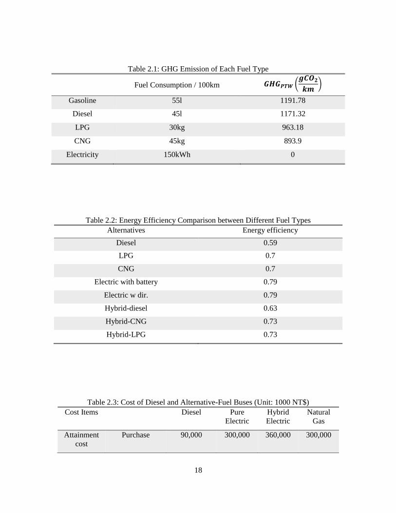
major source of producing GHG, but also are less energy efficiency. Table 2.1 shows t h e
fuel consumption and GHG emission rate for each fuel type, where the LPG is liquefied

6
petroleum gas and CNG is compressed natural gas [13]. More importantly, the population
in China is highly concentrated in city area, severe traffic congestion occurs in two peak
periods every day. [14] shows that as traffic congestion increases, so do fuel consumption
and GHG emissions. Table 2.2 gives the energy efficiency values based on multi-criteria
analysis by [15]. In this table, higher value means better fuel efficiency. Diesel-powered
buses have the lowest energy efficiency values comparing to alternative fuel vehicles.
Therefore, with the progress of bus replacement project, conventional diesel buses should be
gradually eliminated since their poor performance in fuel economy and are less
environmental friendly. However, the new project requires tremendous capital and relatively
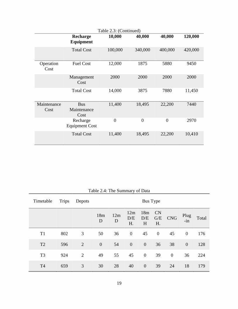
longer periods to implement. Data in Table 2.3 published by Institute of Transportation (2000)
indicates that the operational costs of AFVs are far less than diesel buses [15]. In fact, AFVs cost
three times more on attainment and twice more on maintenance than the conventional diesel
buses. At present, public transit provider is seeking solutions to optimally utilize both
conventional diesel buses and alternative fuel vehicles on their daily service schedules.
2.3 Model and Methods
2.3.1 Vehicle Scheduling Problem
The bus scheduling problem in public transportation involves a set of timetabled trips
with start/end stations, trip durations, lengths and depot numbers, given the capacity of depots,
the objective is to find an optimal schedule so that total costs is minimized. The operational costs
usually refer to the cost incurred by buses running on deadhead trips. Deadhead trips are the
movement of an empty vehicle from the end station of a finished trip to the start station of an
upcoming trip or from/to depot. In traditional bus scheduling problem, costs are calculated only
based on the distances. Costs variation of different types of buses running on same trips are not

7
considered explicitly. In practice, attainment and maintenance costs should not be overlooked.
As we mentioned, they vary considerably among vehicles. Additionally, due to special situation
in China, the duration of trips with the same distances is highly influenced by the traffic patterns.
Therefore, the various costs should be considered and modeled explicitly in AFV scheduling.
Vehicle scheduling problem is well recognized as complicated problem due to its
numerous possibilities to assign vehicle to each trip, to schedule sequences of service trips for
each bus, and to assign buses to depots. Multi-depot vehicle scheduling problem is well-known
as the NP-hard problem [16]. With the increase of the number of trips and depots, the problem
size can grow exponentially. Therefore, standard solvers cannot handle instances with thousands
of trips.
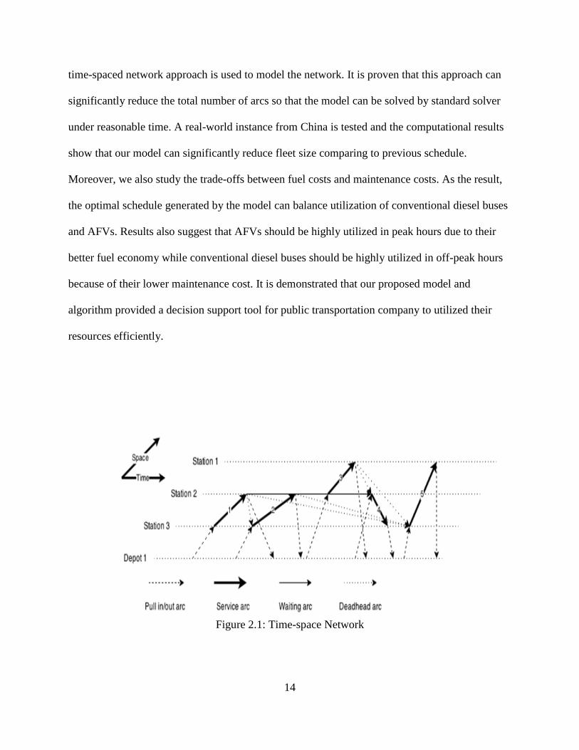
2.3.2 Time-space Network
[17] first proposed a time-space network model for routing problems in airline schedule
application. The same approach has not been applied in vehicle scheduling until recently. [18]
applied the technique to the multi-depot vehicle scheduling in 2006. In Kliewer's approach, the
arcs are aggregated and total number of arcs are highly reduced. Figure 2.1 shows the proposed
time-space network. Arcs in this network can be categorized as follows:
1. Pull-in/pull-out arcs: Buses pull out from depots to serve scheduled trips, or pull in from
finished trips to depots.
2. Service trip arcs: The timetabled or scheduled trips.
3. Waiting arcs: Buses waiting in a station before serving next trips.
4. Deadhead arcs: The movements of empty buses traveling from finished trips to next
scheduled trips.
8
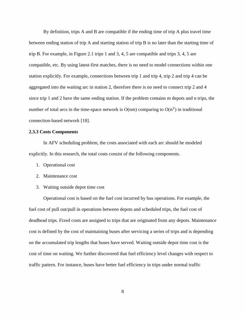
By definition, trips A and B are compatible if the ending time of trip A plus travel time
between ending station of trip A and starting station of trip B is no later than the starting time of
trip B. For example, in Figure 2.1 trips 1 and 3, 4, 5 are compatible and trips 3, 4, 5 are
compatible, etc. By using latest-first matches, there is no need to model connections within one
station explicitly. For example, connections between trip 1 and trip 4, trip 2 and trip 4 can be
aggregated into the waiting arc in station 2, therefore there is no need to connect trip 2 and 4
since trip 1 and 2 have the same ending station. If the problem contains m depots and n trips, the
number of total arcs in the time-space network is O(nm) comparing to O(n2) in traditional
connection-based network [18].
2.3.3 Costs Components
In AFV scheduling problem, the costs associated with each arc should be modeled
explicitly. In this research, the total costs consist of the following components.
1. Operational cost
2. Maintenance cost
3. Waiting outside depot time cost
Operational cost is based on the fuel cost incurred by bus operations. For example, the
fuel cost of pull out/pull in operations between depots and scheduled trips, the fuel cost of
deadhead trips. Fixed costs are assigned to trips that are originated from any depots. Maintenance
cost is defined by the cost of maintaining buses after servicing a series of trips and is depending
on the accumulated trip lengths that buses have served. Waiting outside depot time cost is the
cost of time on waiting. We further discovered that fuel efficiency level changes with respect to
traffic pattern. For instance, buses have better fuel efficiency in trips under normal traffic

9
conditions than those under heavy traffic conditions. Therefore, fuel economies vary according
to specific traffic patterns.
2.3.4 Mathematical Formulation
We define T as the set of timetabled trips, D the set of depots, L the set of bus types.
𝑖, 𝑗 ∈ 𝑇 ∪ 𝐷 represent the timetabled trip, 𝑑 ∈ 𝐷 represents depot, 𝑙 ∈ 𝐿 denotes bus type. Each
trip has its corresponding start and end stations, denoted by 𝑠𝑘𝑖 , 𝑒𝑘𝑖, start and end times, denoted
by 𝑠𝑡𝑖 , 𝑒𝑡𝑖, as well as trip distances 𝑡𝑑𝑖. We construct a vehicle scheduling network 𝐺𝐷 =
(𝑉𝐷, 𝐴𝐷) for each depot, with nodes 𝑉𝐷 = 𝑉𝑇 ∪ 𝑉𝑑 and arcs 𝐴𝐷 = 𝐴𝑇 ∪ 𝐴𝑑, where the set of
nodes 𝑉𝐷 denotes service trip nodes 𝑉𝑇 and depot nodes 𝑉𝑑, 𝐴𝑑 connect depot d and trips starting
from it. Deadhead arcs are denoted by 𝐴𝑇.
We also define 𝑄𝑑𝑙 as the number of available buses in type 𝑙 at depot d, 𝐾𝑑 as the
capacity of depot d and 𝑢𝑙 as the fuel price of bus type l. For total costs, we let 𝐶𝑖𝑗𝑑𝑙 represents the
cost of buses traveling from end station of trip i to the start station of trip j plus operational cost
for serving trip i. F is the fixed cost of operating a new bus. 𝑤𝑜𝑐 denotes the waiting time spent
outside depot to serve next trip. ℎ𝑖𝑗 be the distances from end station of trip i to the start station
of trip j or distances between depots and trips. Let 𝜌 be the traffic pattern indicator denotes the
level of traffic congestion. 𝐹𝐸𝑙 be the fuel efficiency of bus type l. We also define 𝑚𝑙 as the
average maintenance cost per unit distance of bus type l. Therefore, 𝐶𝑖𝑗𝑑𝑙 can be calculated as
follows:
1. When i, j are both service trips and end station of i is different from start station of j,
𝐶𝑖𝑗𝑑𝑙 = 𝜌 ∗ 𝑢𝑙 ∗ (𝑡𝑑𝑖 + ℎ𝑖𝑗)/𝐹𝐸𝑙 + 𝑚𝑙(ℎ𝑖𝑗 + 𝑡𝑑𝑖) + 𝑤𝑜𝑐 ∗ (𝑠𝑡𝑗 − 𝑒𝑡𝑖) (1)
2. Similarly, when i, j are trips and end station of i and start station of j are equal,

10
𝐶𝑖𝑗𝑑𝑙 = 𝜌 ∗ 𝑢𝑙 ∗ 𝑡𝑑𝑖/𝐹𝐸𝑙 + 𝑚𝑙 ∗ 𝑡𝑑𝑖 + 𝑤𝑜𝑐 ∗ (𝑠𝑡𝑗 − 𝑒𝑡𝑖) (2)
3. When i is depot and j is service trip,
𝐶𝑖𝑗𝑑𝑙 = 𝐹 + 𝜌 ∗ 𝑢𝑙 ∗ ℎ𝑖𝑗/𝐹𝐸𝑙 + 𝑚𝑙 ∗ ℎ𝑖𝑗 (3)
4. When i is trip and j is depot,
𝐶𝑖𝑗𝑑𝑙 = 𝜌 ∗ 𝑢𝑙 ∗ ℎ𝑖𝑗/𝐹𝐸𝑙 + 𝑚𝑙 ∗ ℎ𝑖𝑗 (4)
Finally, we let 𝑥𝑖𝑗𝑑𝑙 be binary variables, with 𝑥𝑖𝑗
𝑑𝑙 = 1 if bus type 𝑙 from depot d serve trip j
after finish trip i, and 𝑥𝑖𝑗𝑑𝑙 = 0 otherwise. Then we propose the multi-depot, multiple vehicle type
alternative fuel vehicle scheduling integer programming model (MDMVSP):
𝑚𝑖𝑛𝑥
∑ ∑ ∑ 𝐶𝑖𝑗𝑑𝑙𝑥𝑖𝑗
𝑑𝑙
𝑖,𝑗∈𝐴𝑇∪𝐴𝑑𝑑∈𝐷l∈L
(5)
𝑠. 𝑡. ∑ 𝑥𝑖𝑗𝑑𝑙
𝑖:(𝑖,𝑗)∈𝐴𝑇∪𝐴𝑑
− ∑ 𝑥𝑖𝑗𝑑𝑙
𝑖:(𝑗,𝑖)∈𝐴𝑇∪𝐴𝑑
= 0, ∀𝑗 ∈ 𝑉𝑇 ∈ 𝑉𝐷 , 𝑑 ∈ 𝑉𝐷 , 𝑙 ∈ 𝐿 (6)
∑ ∑ ∑ 𝑥𝑖𝑗𝑑𝑙
𝑗∈𝑉𝑇∪𝑉𝐷𝑑∈𝐷𝑙∈𝐿
= 1, ∀𝑖 ∈ 𝑉𝑇 (7)
∑ ∑ 𝑥𝑖𝑗𝑑𝑙
𝑗:(𝑖,𝑗)∈𝐴𝑇
≤ 𝐾𝑑
𝑙∈𝐿
, ∀𝑑 ∈ 𝑉𝐷, 𝑖 ∈ 𝑉𝐷 (8)
∑ 𝑥𝑖𝑗𝑑𝑙
𝑗:(𝑖,𝑗)∈𝐴𝑑
≤ 𝑄𝑑𝑙 , ∀𝑖 ∈ 𝑉𝐷 , 𝑙 ∈ 𝐿, 𝑑 ∈ 𝑉𝐷 (9)
𝑥𝑖𝑗𝑑𝑙 = {0,1}, ∀(𝑖, 𝑗) ∈ 𝐴𝑇 ∪ 𝐴𝑑 , 𝑑 ∈ 𝐷, 𝑙 ∈ 𝐿 (10)
The objective function (5) in MDMVSP model seeks to minimize the sum of the total
costs. Constraints (6) are the flow conservation constraints, representing that the out-flow and in-
flow of each node should be equal, constraints (7) indicates that each trip should only be served
by one bus of type l from depot d, (8) and (9) are the depot and vehicle type capacity constraints
respectively.

11
2.4 Numerical Study
In this study, we collaborate with a public transit company, Zhengzhou Bus
Communication Company (ZZBC) in Zhengzhou, Henan, China. The real-world data is obtained
from ZZBC's database, including bus routes, bus types, scheduled timetables and depot
information. There are total of 17 Bus Rapid Transit (BRT) routes with two directions and they
are grouped into 4 categories based on their service range. Four timetables were obtained and
denoted by T1 to T4, with their corresponding number of trips and depots. Each timetable
contains a combination of bus routes with different vehicle-type availability. There are 7 types of
bus in total, we treat 18m Diesel and 12m Diesel as two distinct types since their fuel efficiency
varies due to differences in length.
The detailed parameters can be seen in Table 2.5. Fuel economy and prices were obtained
from ZZBC based on a report conducted by Grutter consulting company [19]. Maintenance cost
was reported by [15] and converted to US dollar per kilometer based on estimated annual
average distances of 55,000 kilometers. We assume that the maintenance costs for buses of the
same type with different lengths are equal. Attainment costs were excluded since we are
optimizing the schedule based on the existing buses and it does not require purchasing new
buses. [20] reported that congestion can take great effects on fuel consumption, and the
simulation shows that an approximate 50 percent increase in fuel consumption under heavily
congested condition. To better capture the traffic congestion patterns, we set 𝜌 to three levels
𝜌 = 1,2,3 representing the congestion levels of light, medium, heavy, respectively. The cost of
bus waiting outside depot for one-minute is set to be 1 and the fixed cost of operating a new bus
to be $1,000. Each depot has a capacity of 100. ZZBC requires that the limit of idle time for
buses waiting outside depot is 20 minutes.
12
The algorithm was implemented in MATLAB R2013a on Lenovo ThinkPad T420s with
Intel Core i5-2520M CPU at 2.50GHz, 8GB of RAM and Windows 7 operating system (64).
C++ and CPLEX 12.5 are used to solve integer programs. Table 2.6 presents the computational
results for the four instances with 𝜌 = 1,2,3 levels of traffic congestion and the number of bus in
each type. Column AFV Utilization is the percentage of alternative fuel vehicles used among
mixed fleet. Column Vehicle Reduction is the percentage of the total number of buses reduced
comparing to the existing schedule. Column cost is the total cost required for each timetable
under different congestion scenarios. Column CPU denotes the solution time.
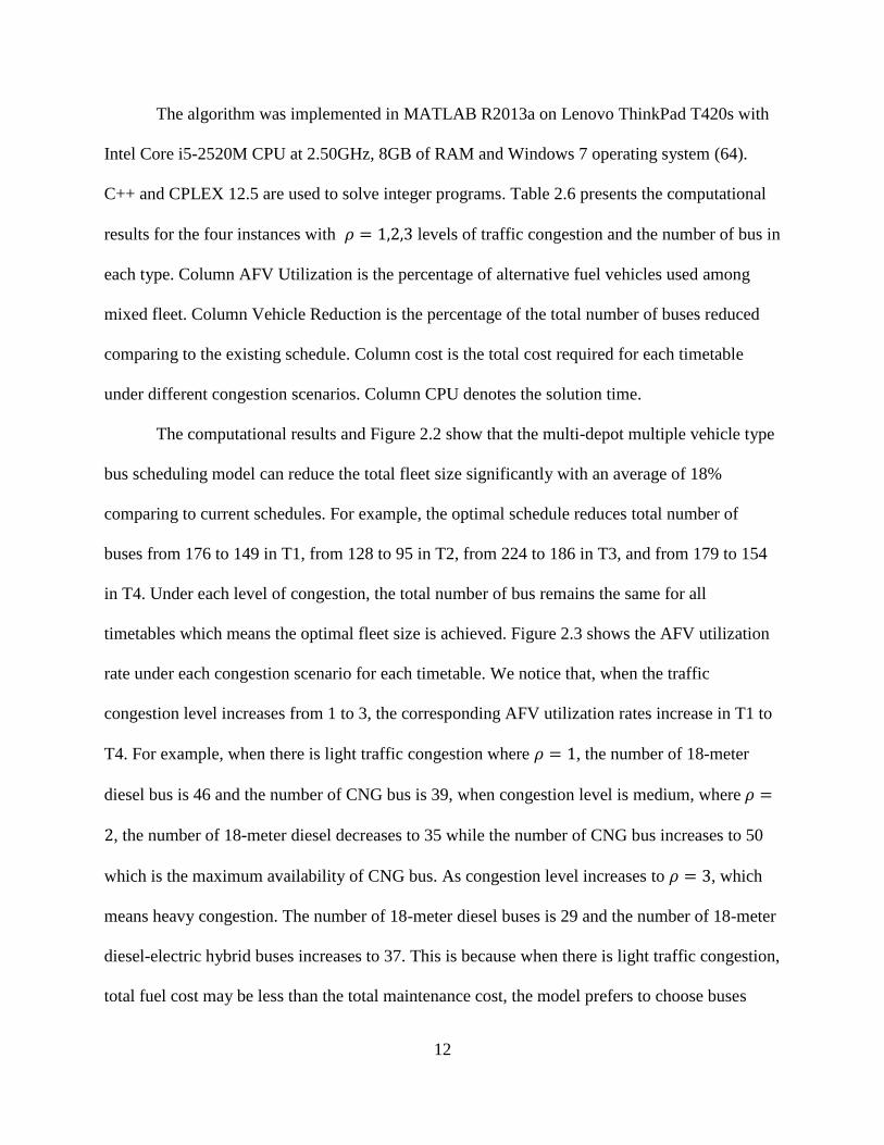
The computational results and Figure 2.2 show that the multi-depot multiple vehicle type
bus scheduling model can reduce the total fleet size significantly with an average of 18%
comparing to current schedules. For example, the optimal schedule reduces total number of
buses from 176 to 149 in T1, from 128 to 95 in T2, from 224 to 186 in T3, and from 179 to 154
in T4. Under each level of congestion, the total number of bus remains the same for all
timetables which means the optimal fleet size is achieved. Figure 2.3 shows the AFV utilization
rate under each congestion scenario for each timetable. We notice that, when the traffic
congestion level increases from 1 to 3, the corresponding AFV utilization rates increase in T1 to
T4. For example, when there is light traffic congestion where 𝜌 = 1, the number of 18-meter
diesel bus is 46 and the number of CNG bus is 39, when congestion level is medium, where 𝜌 =
2, the number of 18-meter diesel decreases to 35 while the number of CNG bus increases to 50
which is the maximum availability of CNG bus. As congestion level increases to 𝜌 = 3, which
means heavy congestion. The number of 18-meter diesel buses is 29 and the number of 18-meter
diesel-electric hybrid buses increases to 37. This is because when there is light traffic congestion,
total fuel cost may be less than the total maintenance cost, the model prefers to choose buses
13
with low maintenance cost. However, when traffic level increases, fuel consumption increases
for the same trips and fuel cost becomes the dominant cost. Hence higher utilization of
alternative fuel vehicle is achieved due to their high fuel efficiency. Figure 2.4 to Figure 2.7
show the comparison of utilization of AFVs in normal and heavy congestion periods trips in
timetable T1 to T4.
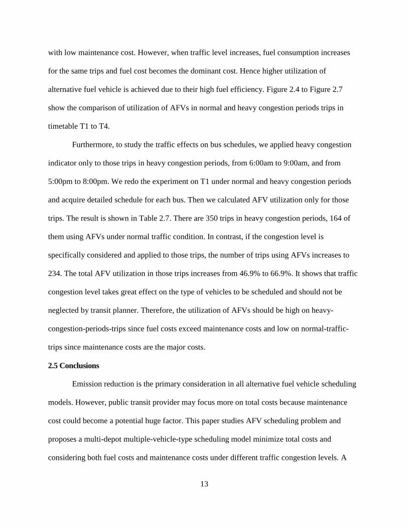
Furthermore, to study the traffic effects on bus schedules, we applied heavy congestion
indicator only to those trips in heavy congestion periods, from 6:00am to 9:00am, and from
5:00pm to 8:00pm. We redo the experiment on T1 under normal and heavy congestion periods
and acquire detailed schedule for each bus. Then we calculated AFV utilization only for those
trips. The result is shown in Table 2.7. There are 350 trips in heavy congestion periods, 164 of
them using AFVs under normal traffic condition. In contrast, if the congestion level is
specifically considered and applied to those trips, the number of trips using AFVs increases to
234. The total AFV utilization in those trips increases from 46.9% to 66.9%. It shows that traffic
congestion level takes great effect on the type of vehicles to be scheduled and should not be
neglected by transit planner. Therefore, the utilization of AFVs should be high on heavy-
congestion-periods-trips since fuel costs exceed maintenance costs and low on normal-traffic-
trips since maintenance costs are the major costs.
2.5 Conclusions
Emission reduction is the primary consideration in all alternative fuel vehicle scheduling
models. However, public transit provider may focus more on total costs because maintenance
cost could become a potential huge factor. This paper studies AFV scheduling problem and
proposes a multi-depot multiple-vehicle-type scheduling model minimize total costs and
considering both fuel costs and maintenance costs under different traffic congestion levels. A
14
time-spaced network approach is used to model the network. It is proven that this approach can
significantly reduce the total number of arcs so that the model can be solved by standard solver
under reasonable time. A real-world instance from China is tested and the computational results
show that our model can significantly reduce fleet size comparing to previous schedule.
Moreover, we also study the trade-offs between fuel costs and maintenance costs. As the result,
the optimal schedule generated by the model can balance utilization of conventional diesel buses
and AFVs. Results also suggest that AFVs should be highly utilized in peak hours due to their
better fuel economy while conventional diesel buses should be highly utilized in off-peak hours
because of their lower maintenance cost. It is demonstrated that our proposed model and
algorithm provided a decision support tool for public transportation company to utilized their
resources efficiently.
Figure 2.1: Time-space Network

15
Figure 2.2: Comparison of Fleet Size in Existing and Optimal Schedules
Figure 2.3: The Utilization of AFVs under Each Scenario

16
Figure 2.4: The Utilization of AFVs in Normal and Heavy Congestion Periods Trips (T1)
Figure 2.5: The Utilization of AFVs in Normal and Heavy Congestion Periods Trips (T2)

17
Figure 2.6: The Utilization of AFVs in Normal and Heavy Congestion Periods Trips (T3)
Figure 2.7: The Utilization of AFVs in Normal and Heavy Congestion Periods Trips (T4)
18
Table 2.1: GHG Emission of Each Fuel Type
Fuel Consumption / 100km 𝑮𝑯𝑮𝑷𝑻𝑾 (
𝒈𝑪𝑶𝟐
𝒌𝒎)
Gasoline 55l 1191.78
Diesel 45l 1171.32
LPG 30kg 963.18
CNG 45kg 893.9
Electricity 150kWh 0
Table 2.2: Energy Efficiency Comparison between Different Fuel Types
Alternatives Energy efficiency
Diesel 0.59
LPG 0.7
CNG 0.7
Electric with battery 0.79
Electric w dir. 0.79
Hybrid-diesel 0.63
Hybrid-CNG 0.73
Hybrid-LPG 0.73
Table 2.3: Cost of Diesel and Alternative-Fuel Buses (Unit: 1000 NT$)
Cost Items Diesel Pure
Electric
Hybrid
Electric
Natural
Gas
Attainment
cost
Purchase 90,000 300,000 360,000 300,000
19
Table 2.3: (Continued)
Recharge
Equipment
10,000 40,000 40,000 120,000
Total Cost 100,000 340,000 400,000 420,000
Operation
Cost
Fuel Cost 12,000 1875 5880 9450
Management
Cost
2000 2000 2000 2000
Total Cost 14,000 3875 7880 11,450
Maintenance
Cost
Bus
Maintenance
Cost
11,400 18,495 22,200 7440
Recharge
Equipment Cost
0 0 0 2970
Total Cost 11,400 18,495 22,200 10,410
Table 2.4: The Summary of Data
Timetable Trips Depots Bus Type
18m
D
12m
D
12m
D/E
H.
18m
D/E
H
CN
G/E
H.
CNG Plug
-in Total
T1 802 3 50 36 0 45 0 45 0 176
T2 596 2 0 54 0 0 36 38 0 128
T3 924 2 49 55 45 0 39 0 36 224
T4 659 3 30 28 40 0 39 24 18 179

20
Table 2.5: Parameters
Bus Type Fuel Economy (100 km) Fuel Price ($) Maintenance
cost ($/km)
FE1 FE2
18m Diesel 66.5 L 99.8 L 1.16 $/L 6.62 $/km
12m Diesel 40.0 L 60.0 L 1.16 $/L 6.62 $/km
12m D/E H. 29.5 L 44.3 L 1.16 $/L 15.89 $/km
18m D/E H. 43.9 L 65.9 L 1.16 $/L 15.89 $/km
CNG/E H. 39 𝑚3 58.5 𝑚3 0.52 $/𝑚3 19.89 $/km
CNG 47.9 𝑚3 71.9 𝑚3 0.52 $/𝑚3 9.04 $/km
Plug-in H. 100 kWh 150 kWh 0.08 $/kWh 26.75 $/km
D: Diesel E: Electric H: Hybrid CNG: Compressed Natural Gas

21
Table 2.6: Computational Results
Congestion
Level Timetable Bus Type
AFV
Utilization
(%)
Vehicle
Reduction
(%)
Cost CPU(s)
18m
D
12m
D
12m
D/E
H.
18m
D/E
H.
CNG/E
H. CNG
Plug-
in H. Total
𝛒 = 𝟏 T1 46 33 0 31 0 39 0 149 31.3 15.3 193873 260.574 T2 0 50 0 0 27 18 0 95 47.4 25.8 119006 73.957
T3 40 55 38 0 39 0 14 186 48.9 17.0 241430 367.598
T4 23 28 40 0 39 24 0 154 66.9 14.0 186472 252.257
𝛒 = 𝟐 T1 35 33 0 31 0 50 0 149 54.4 15.3 211477 262.994 T2 0 41 0 0 36 18 0 95 56.8 25.8 129052 75.506
T3 26 55 38 0 39 0 28 186 56.5 17.0 252009 600.261
T4 9 28 40 0 39 24 14 154 75.9 14.0 187629 265.377
𝛒 = 𝟑 T1 29 33 0 37 0 50 0 149 58.4 15.3 226777 256.975 T2 0 22 0 0 36 37 0 95 76.8 25.8 152832 77.93
T3 26 42 43 0 39 0 36 186 63.4 17.0 260301 472.72
T4 9 27 40 0 39 24 15 154 76.6 14.0 196897 264.975
Table 2.7: AFV Utilization of Trips in Peak Hours
Congestion
Level (𝛒) No. of Buses Total Trips
Trips using
AFVs
Utilization
(%)
18m Diesel 12m Diesel 18m D/E H. Plug-in H.
𝛒 = 𝟏 33 46 31 39 350 164 46.9
𝛒 = 𝟑 33 39 31 46 350 234 66.9

22
CHAPTER 3: AMBULANCE LOCATION AND RELOCATION THROUGH TWO
STAGE ROBUST OPTIMIZATION
3.1 Introduction
Emergency Medical Services (EMS) is a necessary, complicated and highly organized
system designed to provide medical care and transportation services under emergency which has
a strongly restricted time frame. The process of intervention of ambulance to the scene in the
incident typically includes four stages: (1) detection and reporting of the incident, (2) emergency
call screening, (3) ambulance dispatching and (4) actual intervention by paramedics [21].
To provide this service to population, a fleet of ambulances need to be located over the
region they serve. The measurement of the quality of service including response times, the types
of care that EMS staffs are trained to provide, and the equipment to which they have access, etc.,
The most important attribute is response time which strongly correlated with patients' survival
rate. Response time in EMS is the time interval from patients calling for service until being
reached. Regulations based on the United States Emergency Medical Services Act of 1973
specified that 95% of calls should be reached within 10 minutes in urban areas, and 30 minutes
in rural areas. [22]. A survey of the 200 largest cities in the United States by [23] indicated that
over 75% of EMS providers use a target of 8:59 min or less as the common response time
standard. Two types of covering constraints were proposed by [24], denoted by 𝑟1 and 𝑟2. In their
notations, 𝑟2 denotes the absolute covering constraints, it ensures all the demand must be covered
by an ambulance within 𝑟2 minutes. More strictly, the relative covering constraints is also

23
introduced. In that constraints, a proportion 𝛼 of the total demand must be covered by ambulance
within 𝑟1 minutes (𝑟2 > 𝑟1). The absolute covering constraint coincides with the United States
EMS Act of 1973 while the relative covering constraint can be determined by EMS service
provider in order to achieve better service standard. Thus, the selection of the emergency medical
service locations is the major issue to the service provider in designing an efficient network. The
goal of emergency medical services is to provide better service coverage for the population and
quicker responses to the service calls, and further increase survival rate of the patients since time
is vital in emergency situations. In general, an emergency medical service call or demand is said
to be covered if they can be reached within a specific time. Hence it is important that ambulances
be at all time located to ensure an adequate coverage and quick response time. [25].
The ambulance location problem has been addressed by many authors previously. Some
focused on the strategic planning, including the system network design. Others emphasized on
the operational support and tactical decisions, for example, dynamically dispatch and relocation.
It is possible that the network components could lose functions and ambulances could
simultaneously become unavailable when disaster or crisis occur, for example, hurricanes in
Florida, tornado in Oklahoma, or even terrorist attack. In recent years, reliability of the service
system has addressed many attentions in terms of maintaining an efficient and effective
emergency medical service network. To hedge uncertainty, more authors study the stochastic
nature of the problem and proposed approaches using either stochastic programming paradigm or
queueing framework. [26], [27], [28], [29], [30], [31]. Those studies either incorporated
probabilistic constraints or used simplified assumptions by embedding the hypercube model or
queueing theory into the mathematical programming models. However, the exact probability
distribution is hard to be characterized by either accurate method or sufficient data in many
24
circumstances. In addition, most of the probabilistic models rely on simplified assumptions that
will cause problems and become impractical in real life. Hence, probabilistic models could be
improper and result in infeasible solutions. Two-stage robust optimization method is introduced
to deal with this issue. In this method, the randomness is simply captured by an uncertainty set so
that robust solutions can be found within the uncertainty set. Therefore, we can make second
stage recourse decision after the uncertainty is identified. The two-stage robust optimization
method has been widely applied in many areas [32], [33], [34], for example the facility location
problems [35].
This study focuses on adopting two-stage robust optimization approach to study reliable
emergency medical service location problem. There is no research study the impact of relocation
operation on initial locations. While in the strategic design stage, the existing probabilistic
models either don't consider relocations or only assign uncovered demand to other nearby
available service sites. [26], [27], [36], [37], [38]. As [39] mentioned, the two-stage robust
optimization modelling framework precisely represents the real decision making processes.
Furthermore, this modelling framework enables us to consider relocation decisions when
designing the network to address uncertainty issues. A customized solution algorithm, i.e.,
column-and-constraint generation method and approximation framework are implemented and
tested on a real-world instance to demonstrate the performance of the algorithm and the network
design modelling framework. The remainder of this chapter is organized as follows. Section 2
presents a review of relevant literature on probabilistic ambulance location models. In Section 3,
two-stage robust optimization emergency medical service location models are proposed. In
Section 4, a customized column-and-constraint generation method and approximation framework
25
is introduced and experiments are tested on a real-world instance. In Section 5, numerical results
are presented and discussed. Conclusions and future research are presented in Section 6.
3.2 Literature Review
Most early studies of the ambulance location problem focused on static and deterministic
location problems. The location set covering model (LSCM) introduced by [40] aims to
minimize total number of ambulances needed to cover all demand points. This model is not
realistic since most of the time all ambulances are not available due to service calls. The
maximal covering location problem (MCLP) was proposed by [41] to counter some of the
shortcomings of the LSCM. Instead of minimize total ambulances needed, MCLP maximizes the
coverage of the demands. Several extensive static models have been developed by [42], [43],
[44] and [24] to consider more aspects, such as different types of service vehicles and additional
backup coverage. In practice, static models are not sufficient to capture the uncertainty of the
operations of emergency services. Demand may become uncovered due to the unavailability of
ambulances once vehicles are dispatched to calls. One way to address this issue is considering
multiple demand coverages. [24] first introduce the double standard model (DSM) and solved by
Tabu search algorithm. [45] modified the DSM to formulate a double-coverage objective
function and single-coverage standard constraints, Tabu Search algorithm was used to find near
optimal solution. Subsequently, [46] developed a dynamic DSM and the model was tested on the
Island of Montreal. [47] introduced a multi-period covering model, considering the fact that
coverage areas change throughout the day. Vehicle reposition are allowed to maintain a certain
coverage standard. A metaheuristic method using variable neighborhood search was
implemented to solve the problem. [48] modified the DSM to maximize the vehicle crash site
coverage with a predefined number of ambulances dedicated to provide EMS services. A genetic
26
algorithm was proposed to solve a real-world problem in the city of Thessaloniki, Greece. An
extension of DSM developed by [49] considers multiple EMS vehicle types and variant coverage
requirements for demand sites with different priority levels. The model was applied for
allocating EMS vehicles in the Chicago urban area.
Another way to address the reliability matter are probabilistic models. One of the first
probabilistic models for ambulance location problem is the maximum expected covering location
problem (MEXCLP) studied by [26]. This model incorporates a busy fraction to represents the
probability of unavailability of each ambulance. An extension of MEXCLP, called TIMEXCLP,
was developed by [27], explicitly considered the variations in travel speed throughout the day.
[36] proposed two other probabilistic models to formulate the maximum availability location
problem (MALP I and MALP II). In MALP I, the busy fraction q is assumed to be the same for
all sites while MALP II assigns different busy fraction to each site. Moreover, several articles
proposed the estimation methods of the busy fraction. [28] developed the adjusted MEXCLP
model (AMEXCLP) assumes that ambulances are not independently operated and the correction
factor has been added to the objective function. Later, [29] proposed the queueing probabilistic
location set covering problem (QPLSCP) to compute the minimum number of ambulances
required to cover a demand point such that the probability of all of them being simultaneously
busy does not exceed a given threshold. The extension of LSCM, called Rel-P, was developed by
[30] incorporated a constraint that ensures the probability that a given demand call will not be
satisfied does not exceed a certain value. A hypercube model was introduced by [50], which is
considered to be capable of computing the busy fraction. Later studies have tried to incorporate
the hypercube model in optimization frameworks for determining the location of emergence
vehicles, such as [51], [52], [53], [54], [55] and [56]. The major drawback of the hypercube

27
model is that its computational complexity grows exponentially in terms of the number of
applied ambulances. Recently, [57] introduced a new stochastic programming model
incorporates probabilistic constraints within the traditional two-stage framework. [56] developed
a new probabilistic coverage model based on MEXCLP and mixed with the hypercube queuing
model. [58] developed two separate models for ambulance location and relocation with
predefined crisis location, models are solved sequentially in three phases.
According to aforementioned models, they all involve very complicated mathematical
programs. Standard solver CPLEX is usually not capable of dealing with large-scale problems,
hence heuristic or exact solution approaches are developed. Those complicated programs require
exact probabilistic information, which is not appropriate in practice. Robust optimization-based
location models not rely on probability distribution, instead, it uses the uncertainty set to capture
all the uncertainty scenarios and search for the robust locations in that uncertainty set [39].
Benders decomposition method is typically used to solve stochastic programming models due to
its strong performance to generate cuts and reduce the feasible region. However, it can’t handle
large-scale practical problems. [59] demonstrates that column-and-constraint generation
algorithm has greater performance in computation comparing to Benders method. This novel
algorithm has been applied to facility location and power scheduling problems. Results show that
the column-and-constraint generation algorithm can solve large-scale problem in very short
time.
In this research, the reliable emergency medical service location design problem is
formulated into the two-stage robust optimization framework. We introduce models with/without
consideration of relocation operations. This unique feature has not been studied in previous
literatures. In addition, we propose customized computational scheme for solving those two-

28
stage robust optimization models. In the relocation model, relocation costs are also considered to
best capture realistic situation. An approximation algorithm on top of the customized scheme is
developed. Experiments are performed on a real-world instance.
3.3 Two-stage Robust EMS Location Models
In this section, a set of two-stage robust ambulance location models with/without the
consideration of relocation are introduced and discussed. As we mentioned, in two-stage robust
optimization framework, an uncertainty set is adopted to represent all the possible uncertainty
scenarios. The worst-case scenarios are then identified and optimal solutions in those cases are
evaluated. In our ambulance location study, we follow the idea in [39] that all ambulances are
homogeneous and we consider all the possible situations with up to k ambulances simultaneously
become unavailable. We then represent the uncertainty set as
𝑩 = {𝒛 ∈ {0,1}|𝑊|: ∑ 𝑧𝑗 ≤ 𝑘
𝑗∈𝑊
} (11)
where 𝑧𝑗 = 1 indicates ambulance at location j is unavailable and 𝑧𝑗 = 0 otherwise. Note that
this compact mathematical form captures an exponential number of scenarios.
3.3.1 Two-stage Robust EMS Location Model without Relocation
In the following, we first propose our two-stage RO EMS location models without
relocation. Let 𝐼 represents the set of demand sites with 𝑑𝑖 being the estimated demand volume,
W represents the set of potential ambulance sites. 𝑝 ambulances need to be placed among those
sites to maximize the coverage. Let 𝑎𝑖𝑗, 𝑏𝑖𝑗 be adjacent matrices where 𝑎𝑖𝑗 = 1 indicates demand
i is covered by site j within 𝑟2 time units and 𝑏ij = 1 indicate site i is covered by site j within 𝑟1
time units, and 𝑎𝑖𝑗 = 𝑏𝑖𝑗 = 0 otherwise. Parameter 𝛼 ∈ [0,1] is introduced as a weight
coefficient to represent our consideration of unavailability situations.
29
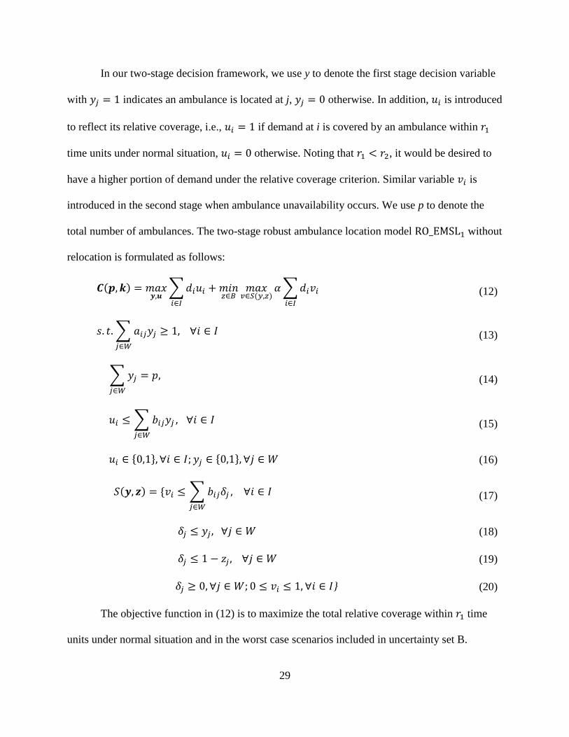
In our two-stage decision framework, we use y to denote the first stage decision variable
with 𝑦𝑗 = 1 indicates an ambulance is located at j, 𝑦𝑗 = 0 otherwise. In addition, 𝑢𝑖 is introduced
to reflect its relative coverage, i.e., 𝑢𝑖 = 1 if demand at i is covered by an ambulance within 𝑟1
time units under normal situation, 𝑢𝑖 = 0 otherwise. Noting that 𝑟1 < 𝑟2, it would be desired to
have a higher portion of demand under the relative coverage criterion. Similar variable 𝑣𝑖 is
introduced in the second stage when ambulance unavailability occurs. We use p to denote the
total number of ambulances. The two-stage robust ambulance location model RO_EMSL1 without
relocation is formulated as follows:
𝑪(𝒑, 𝒌) = 𝑚𝑎𝑥𝒚,𝒖
∑ 𝑑𝑖𝑢𝑖
𝑖∈𝐼
+ 𝑚𝑖𝑛𝑧∈𝐵
𝑚𝑎𝑥𝑣∈𝑆(𝑦,𝑧)
𝛼 ∑ 𝑑𝑖𝑣𝑖
𝑖∈𝐼
(12)
𝑠. 𝑡. ∑ 𝑎𝑖𝑗𝑦𝑗
𝑗∈𝑊
≥ 1, ∀𝑖 ∈ 𝐼 (13)
∑ 𝑦𝑗
𝑗∈𝑊
= 𝑝, (14)
𝑢𝑖 ≤ ∑ 𝑏𝑖𝑗𝑦𝑗
𝑗∈𝑊
, ∀𝑖 ∈ 𝐼 (15)
𝑢𝑖 ∈ {0,1}, ∀𝑖 ∈ 𝐼; 𝑦𝑗 ∈ {0,1}, ∀𝑗 ∈ 𝑊 (16)
𝑆(𝒚, 𝒛) = {𝑣𝑖 ≤ ∑ 𝑏𝑖𝑗𝛿𝑗
𝑗∈𝑊
, ∀𝑖 ∈ 𝐼 (17)
𝛿𝑗 ≤ 𝑦𝑗 , ∀𝑗 ∈ 𝑊 (18)
𝛿𝑗 ≤ 1 − 𝑧𝑗 , ∀𝑗 ∈ 𝑊 (19)
𝛿𝑗 ≥ 0, ∀𝑗 ∈ 𝑊; 0 ≤ 𝑣𝑖 ≤ 1, ∀𝑖 ∈ 𝐼} (20)
The objective function in (12) is to maximize the total relative coverage within 𝑟1 time
units under normal situation and in the worst case scenarios included in uncertainty set B.

30
Constraint (13) imposes that for every demand site, at least 1 ambulances is located within its 𝑟2
time-unit neighborhood. Constraint (14) defines the total number of ambulances equals p.
Constraint (15) indicates that 𝑢𝑖 = 0 if there is no ambulance located within 𝑟1 time units of
demand site i, and 𝑢𝑖 = 1 otherwise. Constraint (17), (18) and (19) indicate that 𝑣𝑖 = 0 if there
is no ambulance available within 𝑟1 time units of demand site i, 𝑣𝑖 = 1 otherwise. Constraint
(20) imposes variable restrictions. Remarks are presented as follows.
1. In this study, we focus on the non-trivial cases where 𝑘 ≤ 𝑝 − 1. Otherwise, in the worst-
case scenario, there is no ambulance available and the problem reduces to maximize the
relative coverage within 𝑟1 time units in the normal situation.
2. It can be easily proven that the optimal value 𝐶(𝑝, 𝑘) is non-decreasing in regard to p;
and non-increasing in regard to k.
In the following section, we present an extension of EMS location model with the
consideration of relocation operations.
3.3.2 Two-stage Robust EMS Location Model with Relocation
In real life, it is not possible to reposition all ambulances when uncertainty situation
occurs, hence the advantage of RO_EMSL1 model is limited to study the importance of those
candidate sites. The two-stage robust EMS location model with relocation is an extension of the
RO_EMSL1 model. As mentioned, when a sufficient coverage cannot be maintained due to
ambulance unavailability, ambulance relocation operations are often implemented to employ
remaining ones to achieve a better coverage. To the best of our knowledge, the impact of
relocation operations on the initial locations in EMS location problem has been paid no attention.
The possible reason is that in those probabilistic models, all of the stochastic scenarios have to be
evaluated, hence the model complexity and solution time increase exponentially with respect to

31
the number of unavailable ambulances. Therefore, it is computationally prohibitive for those
models to capture all the possibilities and be solved in a reasonable time.
In RO_EMSL2, variable 𝑃𝑖𝑗 = 1 represents relocating ambulance from site j to i, 𝑃𝑖𝑗 = 0
otherwise. Variable 𝑞𝑗 = 1 denotes the case where an ambulance stays at site j (after
relocations), 𝑞𝑗 = 0 otherwise. 𝛽 is the relocation cost coefficient which represents the system
decision maker's attitude towards relocation cost. Also, D is the distance matrix. The two-stage
robust EMS location model RO_EMSL2 with relocation is shown as follows:
𝑪𝒓(𝒑, 𝒌) = 𝑚𝑎𝑥𝒚,𝒖
∑ 𝑑𝑖𝑢𝑖
𝑖∈𝐼
+ 𝑚𝑖𝑛𝑧∈𝐵
𝑚𝑎𝑥(𝑷,𝒒,𝒗)∈𝑆𝑟(𝒚,𝒛)
(𝛼 ∑ 𝑑𝑖𝑣𝑖
𝑖∈𝐼
− 𝛽 ∑ ∑ 𝐷𝑖𝑗𝑃𝑖𝑗
𝑗∈𝑊𝑖∈𝑊
) (21)
𝑠. 𝑡. (13) − (16)
𝑆𝑟(𝒚, 𝒛) = {𝑣𝑖 ≤ ∑ 𝑏𝑖𝑗𝑞𝑗
𝑗∈𝑊
, ∀𝑖 ∈ 𝐼 (22)
∑ 𝑃𝑖𝑗
𝑗∈𝑊
≥ 𝑞𝑗 , ∀𝑖 ∈ 𝑊 (23)
𝑃𝑖𝑗 ≤ 1 − 𝑧𝑗 , ∀𝑖, 𝑗 ∈ 𝑊 (24)
𝑃𝑖𝑗 ≤ 𝑦𝑗 , ∀𝑖, 𝑗 ∈ 𝑊 (25)
∑ 𝑃𝑖𝑗
i
≤ 1, ∀𝑗 ∈ 𝑊 (26)
∑ 𝑃𝑖𝑗
j
≤ 1, ∀𝑖 ∈ 𝑊 (27)
𝑃𝑖𝑗 ∈ {0,1}; 0 ≤ 𝑣𝑖 ≤ 1, ∀𝑖 ∈ 𝐼; 0 ≤ 𝑞𝑗 ≤ 1, ∀𝑗 ∈ 𝑊} (28)
The objective function in (21) maximize total relative coverage within 𝑟1 time units under
normal situation and in the worst-case scenarios included in uncertainty set B, cost penalty based
on distances is considered. Constraint (22) defines upper bound of 𝑣𝑖, which depends on the

32
status of 𝑞𝑗 for site j within 𝑟1 time units. Constraint (23) indicates the relation between 𝑃𝑖𝑗 and
𝑞𝑖. Note that 𝑞𝑖 = 0 if there is no ambulance moving to 𝑖. Constraints (24) and (25) ensure that
relocation operation does not occur if no ambulance available at site j. And constraint (26) and
(27) guarantee that the ambulance at j can only be relocated to one site and one site can only host
one ambulance. Constraint (28) imposes variable restrictions. Remarks are presented as follows:
1. It also can be easily proven that the optimal value 𝐶𝑟(𝑝, 𝑘) is non-decreasing with respect
to p; and non-increasing with respect to k.
2. Since binary variables are introduced in the second stage problem, the recourse problem
is a mixed integer program (MIP), standard column-and-constraint generation method is
not applicable. Hence, we seek to extend the column-and-constraint generation in an
approximation framework to achieve a balance between the solution quality and
computational speed.
3.4 Computation Algorithm for Two-stage Robust Optimization Models
In this section, we present the implementation of the computational algorithms for both
RO_EMSL1 and RO_EMSL2 models. We first describe the Column-and-constraint generation
method which is a two level procedure involving computing master problem (MP) and
subproblem (SP). In master problem, we consider a small subset B and build an MIP model with
recourse problems for each individual scenario of this subset. Its optimal value provides an upper
bound. Then, a lower bound can be derived from the subproblem. Once upper bound and lower
bound match, we can conclude that 𝒚∗ provides optimal locations for ambulances.
3.4.1 Implementation of 𝐑𝐎_𝐄𝐌𝐒𝐋𝟏 Model
Notice that, the third level problem of RO_EMSL1 model is a linear program, by applying
the strong duality, we could transform the third level problem by finding its dual problem to a
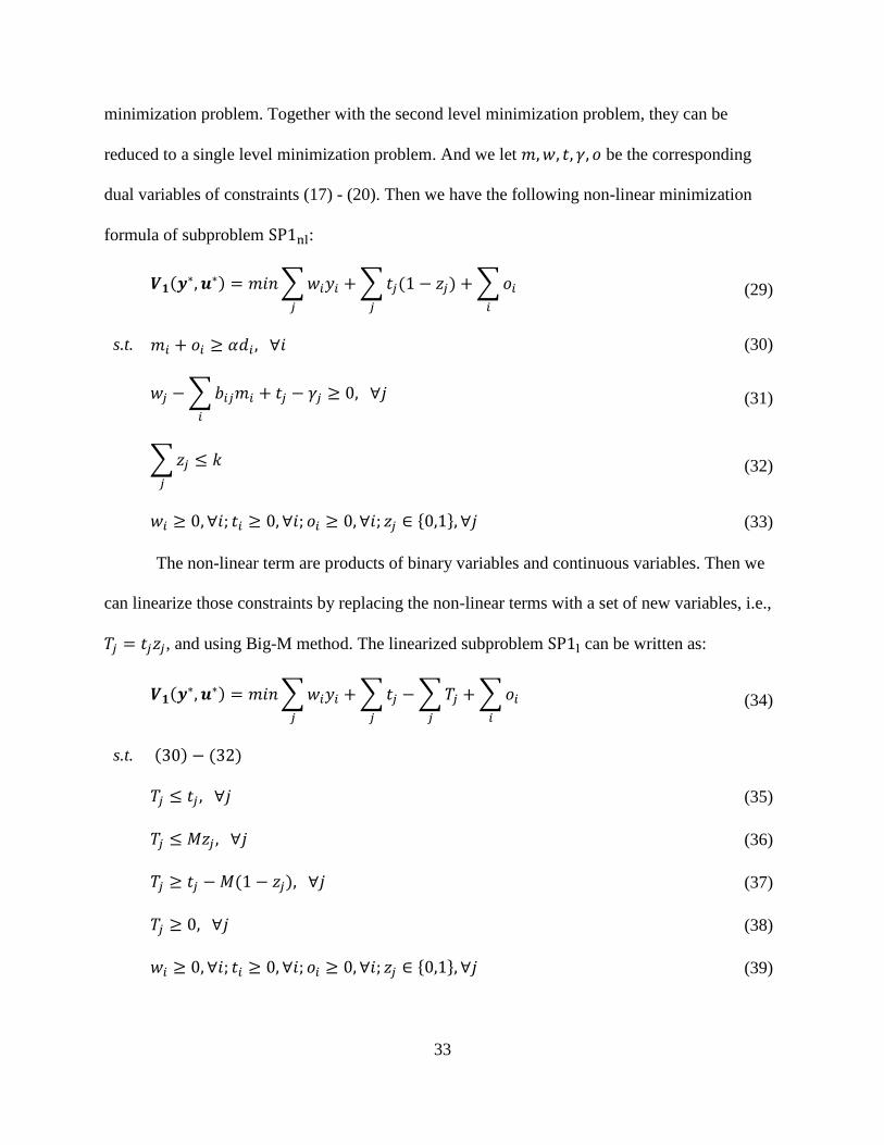
33
minimization problem. Together with the second level minimization problem, they can be
reduced to a single level minimization problem. And we let 𝑚, 𝑤, 𝑡, 𝛾, 𝑜 be the corresponding
dual variables of constraints (17) - (20). Then we have the following non-linear minimization
formula of subproblem SP1nl:
𝑽𝟏(𝒚∗, 𝒖∗) = 𝑚𝑖𝑛 ∑ 𝑤𝑖𝑦𝑖
𝑗
+ ∑ 𝑡𝑗(1 − 𝑧𝑗)
𝑗
+ ∑ 𝑜𝑖
𝑖
(29)
s.t. 𝑚𝑖 + 𝑜𝑖 ≥ 𝛼𝑑𝑖 , ∀𝑖 (30)
𝑤𝑗 − ∑ 𝑏𝑖𝑗𝑚𝑖
𝑖
+ 𝑡𝑗 − 𝛾𝑗 ≥ 0, ∀𝑗 (31)
∑ 𝑧𝑗
𝑗
≤ 𝑘 (32)
𝑤𝑖 ≥ 0, ∀𝑖; 𝑡𝑖 ≥ 0, ∀𝑖; 𝑜𝑖 ≥ 0, ∀𝑖; 𝑧𝑗 ∈ {0,1}, ∀𝑗 (33)
The non-linear term are products of binary variables and continuous variables. Then we
can linearize those constraints by replacing the non-linear terms with a set of new variables, i.e.,
𝑇𝑗 = 𝑡𝑗𝑧𝑗, and using Big-M method. The linearized subproblem SP1l can be written as:
𝑽𝟏(𝒚∗, 𝒖∗) = 𝑚𝑖𝑛 ∑ 𝑤𝑖𝑦𝑖
𝑗
+ ∑ 𝑡𝑗
𝑗
− ∑ 𝑇𝑗
𝑗
+ ∑ 𝑜𝑖
𝑖
(34)
s.t. (30) − (32)
𝑇𝑗 ≤ 𝑡𝑗 , ∀𝑗 (35)
𝑇𝑗 ≤ 𝑀𝑧𝑗 , ∀𝑗 (36)
𝑇𝑗 ≥ 𝑡𝑗 − 𝑀(1 − 𝑧𝑗), ∀𝑗 (37)
𝑇𝑗 ≥ 0, ∀𝑗 (38)
𝑤𝑖 ≥ 0, ∀𝑖; 𝑡𝑖 ≥ 0, ∀𝑖; 𝑜𝑖 ≥ 0, ∀𝑖; 𝑧𝑗 ∈ {0,1}, ∀𝑗 (39)
34
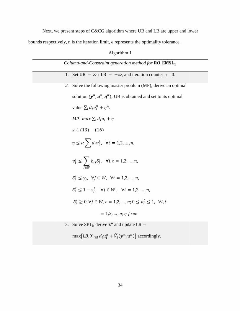
Next, we present steps of C&CG algorithm where UB and LB are upper and lower
bounds respectively, n is the iteration limit, ϵ represents the optimality tolerance.
Algorithm 1
Column-and-Constraint generation method for 𝐑𝐎_𝐄𝐌𝐒𝐋𝟏
1. Set UB = ∞ ; LB = −∞, and iteration counter n = 0.
2. Solve the following master problem (MP), derive an optimal
solution (𝒚𝒏, 𝒖𝒏, 𝜼𝒏), UB is obtained and set to its optimal
value ∑ 𝑑𝑖𝑢𝑖𝑛 + 𝜂𝑛
𝑖 .
MP: 𝑚𝑎𝑥 ∑ 𝑑𝑖𝑢𝑖 + 𝜂𝑖
𝑠. 𝑡. (13) − (16)
𝜂 ≤ 𝛼 ∑ 𝑑𝑖𝑣𝑖𝑡
𝑖
, ∀𝑡 = 1,2, … , 𝑛,
𝑣𝑖𝑡 ≤ ∑ 𝑏𝑖𝑗𝛿𝑗
𝑡
𝑗∈𝑊
, ∀𝑖, 𝑡 = 1,2, … , 𝑛,
𝛿𝑗𝑡 ≤ 𝑦𝑗 , ∀𝑗 ∈ 𝑊, ∀𝑡 = 1,2, … , 𝑛,
𝛿𝑗𝑡 ≤ 1 − 𝑧𝑗
𝑡, ∀𝑗 ∈ 𝑊, ∀𝑡 = 1,2, … , 𝑛,
𝛿𝑗𝑡 ≥ 0, ∀𝑗 ∈ 𝑊, 𝑡 = 1,2, … , 𝑛; 0 ≤ 𝑣𝑖
𝑡 ≤ 1, ∀𝑖, 𝑡
= 1,2, … , 𝑛; 𝜂 𝑓𝑟𝑒𝑒
3. Solve SP1l, derive 𝐳𝐨 and update LB =
max{𝐿𝐵, ∑ 𝑑𝑖𝑢𝑖𝑛
𝑖∈𝐼 + 𝑉1(𝑦𝑛, 𝑢𝑛)} accordingly.
35
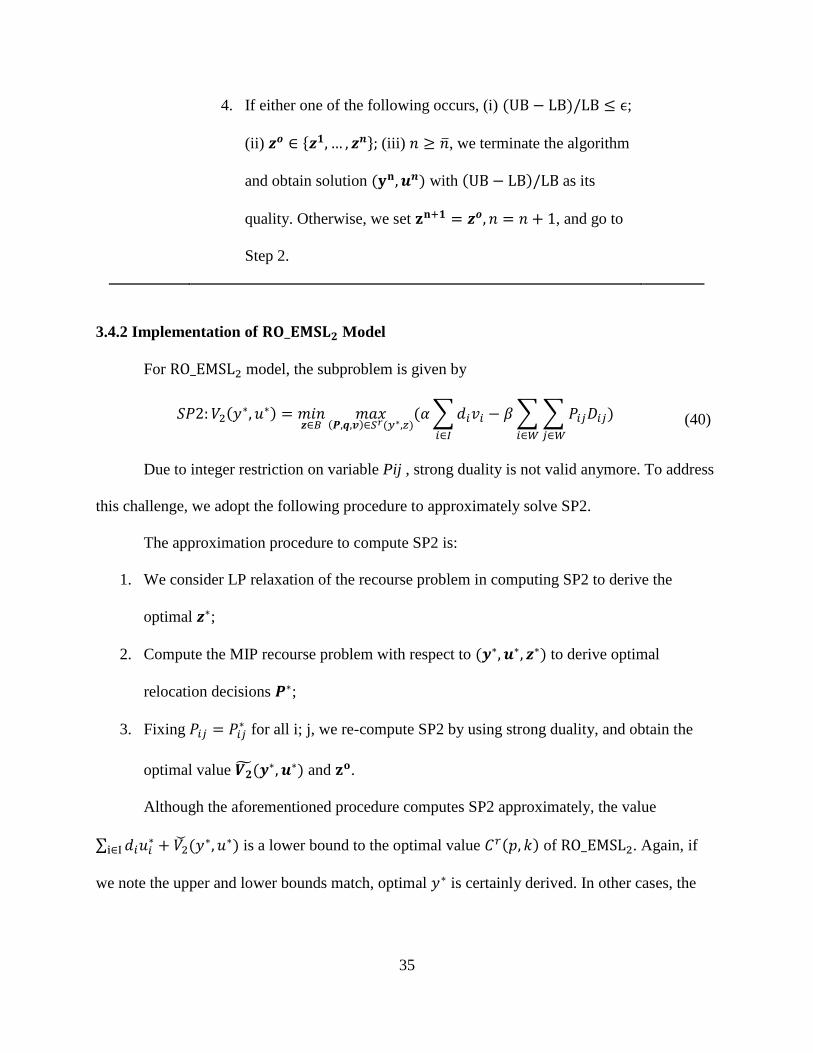
4. If either one of the following occurs, (i) (UB − LB)/LB ≤ ϵ;
(ii) 𝒛𝒐 ∈ {𝒛𝟏, … , 𝒛𝒏}; (iii) 𝑛 ≥ ��, we terminate the algorithm
and obtain solution (𝐲𝐧, 𝒖𝒏) with (UB − LB)/LB as its
quality. Otherwise, we set 𝐳𝐧+𝟏 = 𝒛𝒐, 𝑛 = 𝑛 + 1, and go to
Step 2.
3.4.2 Implementation of 𝐑𝐎_𝐄𝐌𝐒𝐋𝟐 Model
For RO_EMSL2 model, the subproblem is given by
𝑆𝑃2: 𝑉2(𝑦∗, 𝑢∗) = 𝑚𝑖𝑛𝒛∈𝐵
𝑚𝑎𝑥(𝑷,𝒒,𝒗)∈𝑆𝑟(𝑦∗,𝑧)
(𝛼 ∑ 𝑑𝑖𝑣𝑖
𝑖∈𝐼
− 𝛽 ∑ ∑ 𝑃𝑖𝑗𝐷𝑖𝑗
𝑗∈𝑊𝑖∈𝑊
) (40)
Due to integer restriction on variable Pij , strong duality is not valid anymore. To address
this challenge, we adopt the following procedure to approximately solve SP2.
The approximation procedure to compute SP2 is:
1. We consider LP relaxation of the recourse problem in computing SP2 to derive the
optimal 𝒛∗;
2. Compute the MIP recourse problem with respect to (𝒚∗, 𝒖∗, 𝒛∗) to derive optimal
relocation decisions 𝑷∗;
3. Fixing 𝑃𝑖𝑗 = 𝑃𝑖𝑗∗ for all i; j, we re-compute SP2 by using strong duality, and obtain the
optimal value 𝑽��(𝒚∗, 𝒖∗) and 𝐳𝐨.
Although the aforementioned procedure computes SP2 approximately, the value
∑ 𝑑𝑖𝑢𝑖∗
i∈I + 𝑉2(𝑦∗, 𝑢∗) is a lower bound to the optimal value 𝐶𝑟(𝑝, 𝑘) of RO_EMSL2. Again, if
we note the upper and lower bounds match, optimal 𝑦∗ is certainly derived. In other cases, the
36
gap between the upper and lower bounds can be used to evaluate the quality of a feasible
solution.
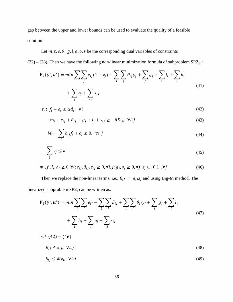
Let 𝑚, 𝑡, 𝑒, 𝜃 , 𝑔, 𝑙, ℎ, 𝑜, 𝑠 be the corresponding dual variables of constraints
(22) – (28). Then we have the following non-linear minimization formula of subproblem SP2nl:
𝑽𝟐(𝒚∗, 𝒖∗) = 𝑚𝑖𝑛 ∑ ∑ 𝑒𝑖𝑗(1 − 𝑧𝑗)
𝑗
+ ∑ ∑ 𝜃𝑖𝑗𝑦𝑗
𝑗𝑖𝑖
+ ∑ 𝑔𝑗
𝑗
+ ∑ 𝑙𝑖
𝑖
+ ∑ ℎ𝑖
𝑖
+ ∑ 𝑜𝑗
𝑗
+ ∑ 𝑠𝑖𝑗
𝑖𝑗
(41)
𝑠. 𝑡. 𝑓𝑖 + 𝑜𝑖 ≥ 𝛼𝑑𝑖 , ∀𝑖 (42)
−mi + 𝑒𝑖𝑗 + 𝜃𝑖𝑗 + 𝑔𝑗 + 𝑙𝑖 + 𝑠𝑖𝑗 ≥ −𝛽𝐷𝑖𝑗 , ∀𝑖, 𝑗 (43)
𝑀𝑖 − ∑ 𝑏𝑖𝑗𝑓𝑖
𝑖
+ 𝑜𝑗 ≥ 0, ∀𝑖, 𝑗 (44)
∑ 𝑧𝑗
j
≤ 𝑘 (45)
𝑚𝑖, 𝑓𝑖 , 𝑙𝑖, ℎ𝑖 ≥ 0, ∀𝑖; 𝑒𝑖𝑗, 𝜃𝑖𝑗 , 𝑠𝑖𝑗 ≥ 0, ∀𝑖, 𝑗; 𝑔𝑗 , 𝑜𝑗 ≥ 0, ∀𝑗; 𝑧𝑗 ∈ {0,1}, ∀𝑗 (46)
Then we replace the non-linear terms, i.e., 𝐸𝑖𝑗 = 𝑒𝑖𝑗𝑧𝑗 and using Big-M method. The
linearized subproblem SP2l can be written as:
𝑽𝟐(𝒚∗, 𝒖∗) = 𝑚𝑖𝑛 ∑ ∑ 𝑒𝑖𝑗
𝑗
− ∑ ∑ 𝐸𝑖𝑗
𝑗𝑖
+ ∑ ∑ 𝜃𝑖𝑗𝑦𝑗
𝑗𝑖𝑖
+ ∑ 𝑔𝑗
𝑗
+ ∑ 𝑙𝑖
𝑖
+ ∑ ℎ𝑖
𝑖
+ ∑ 𝑜𝑗
𝑗
+ ∑ 𝑠𝑖𝑗
𝑖𝑗
(47)
𝑠. 𝑡. (42) − (46)
𝐸𝑖𝑗 ≤ 𝑒𝑖𝑗 , ∀𝑖, 𝑗 (48)
𝐸𝑖𝑗 ≤ 𝑀𝑧𝑗 , ∀𝑖, 𝑗 (49)
37
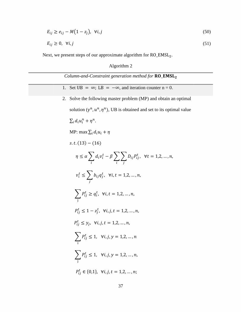
𝐸𝑖𝑗 ≥ 𝑒𝑖𝑗 − 𝑀(1 − 𝑧𝑗), ∀𝑖, 𝑗 (50)
𝐸𝑖𝑗 ≥ 0, ∀𝑖, 𝑗 (51)
Next, we present steps of our approximate algorithm for RO_EMSL2.
Algorithm 2
Column-and-Constraint generation method for 𝐑𝐎_𝐄𝐌𝐒𝐋𝟐
1. Set UB = ∞; LB = −∞, and iteration counter n = 0.
2. Solve the following master problem (MP) and obtain an optimal
solution (yn, 𝑢𝑛, 𝜂𝑛), UB is obtained and set to its optimal value
∑ 𝑑𝑖𝑢𝑖𝑛 + 𝜂𝑛
i .
MP: max ∑ 𝑑𝑖𝑢𝑖 + 𝜂i
𝑠. 𝑡. (13) − (16)
𝜂 ≤ 𝛼 ∑ 𝑑𝑖𝑣𝑖𝑡
𝑖
− 𝛽 ∑ ∑ 𝐷𝑖𝑗𝑃𝑖𝑗𝑡
𝑗𝑖
, ∀𝑡 = 1,2, … , 𝑛,
𝑣𝑖𝑡 ≤ ∑ 𝑏𝑖𝑗𝑞𝑗
𝑡
𝑗
, ∀𝑖, 𝑡 = 1,2, … , 𝑛,
∑ 𝑃𝑖𝑗𝑡
j
≥ 𝑞𝑖𝑡, ∀𝑖, 𝑡 = 1,2, … , 𝑛,
𝑃𝑖𝑗𝑡 ≤ 1 − 𝑧𝑗
𝑡, ∀𝑖, 𝑗, 𝑡 = 1,2, … , 𝑛,
𝑃𝑖𝑗𝑡 ≤ 𝑦𝑗 , ∀𝑖, 𝑗, 𝑡 = 1,2, … , 𝑛,
∑ 𝑃𝑖𝑗𝑡 ≤ 1,
i
∀𝑖, 𝑗, 𝑦 = 1,2, … , 𝑛
∑ 𝑃𝑖𝑗𝑡 ≤ 1,
j
∀𝑖, 𝑗, 𝑦 = 1,2, … , 𝑛,
𝑃𝑖𝑗𝑡 ∈ {0,1}, ∀𝑖, 𝑗, 𝑡 = 1,2, … , 𝑛;
38
0 ≤ 𝑣𝑖𝑡 ≤ 1, ∀𝑗, 𝑡 = 1,2, … , 𝑛,
0 ≤ 𝑞𝑗𝑡 ≤ 1, ∀𝑗, 𝑡 = 1,2, … , 𝑛; 𝜂 𝑓𝑟𝑒𝑒
3. Solve SP2l by the approximation procedure, derive 𝑧𝑜 and
update 𝐿𝐵 = 𝑚𝑎𝑥{𝐿𝐵, ∑ 𝑑𝑖𝑢𝑖𝑛
𝑖∈𝐼 + 𝑉1(𝑦𝑛, 𝑢𝑛)} accordingly.
4. If either one of the following occurs, (i) (UB − LB)/LB ≤ ϵ; (ii)
𝑧𝑜 ∈ {𝑧1, … , 𝑧𝑛}; (iii) n ≥ ��, we terminate the algorithm and
obtain solution (yn, 𝑢𝑛) with (UB − LB)\LB as its quality.
Otherwise, we set zn+1 = 𝑧𝑜 , 𝑛 = 𝑛 + 1, and go to Step 2.
3.5 Numerical Study
In this section, the description on a real-world data is introduced first. Followed by
experimental setup. Then, the results are illustrated and discussed to produce insights on those
robust EMS location models.
3.5.1 Data Description and Computational Experiments
For our computational experiments, we used real-world data from the city of Tampa
(Florida, USA). The demand site information, including population and coordinates are obtained
using census tract data from [60]. There are total of 171 census tracts in Tampa CCD with
population ranging between 0 and 9162. Demand are represented by the probability of calls that
are proportional to the population. Two datasets with 30 and 50 potential sites were randomly
generated. For simplicity, we used the Euclidean distance between any two sites. The maps are
presented in Figure 3.1 and Figure 3.2.
In our study, 𝑟1 is set to 10 minutes and 𝑟2 is set to 12 minutes assuming a constant
vehicle speed of 60 MPH. Also, we set Gap = 0.05 and time limit to 60 minutes. Models and
39
algorithms are implemented in C++ on a Dell OptiPlex 7020 desktop computer (Intel Core i7-
4790 CPU, 3.60 GHz, 16 GB of RAM) in Windows 7 environment. We use a mixed integer
programming solver, CPLEX 12.5 to solve the master problems and subproblems.
3.5.2 Computational Results of 𝐑𝐎_𝐄𝐌𝐒𝐋𝟏 Model
Table 3.1 shows the computational results of RO_EMSL1 model. In this table, column
Time (s) is the computational time in seconds; column Iter represents the number of iterations;
column Obj is the best optimal value ever found; column Gap (%) indicates the relative gap in
percentage if it is larger than ϵ. From Table 3.1, we observe that all the instances can be solved
within time limit and limited iterations. This indicates that the C&CG algorithm has a superior
performance in solving reliable ambulance location problem. Table 3.2 shows the optimal
locations for different scenarios.
3.5.3 Computational Results of 𝐑𝐎_𝐄𝐌𝐒𝐋𝟐 Model
Table 3.3 shows the computational results of RO_EMSL2 model. From the table, we
observe that most of the instances can be solved within very short time and limited iterations.
The computation complexity increases with respect to p, k.
Next, we demonstrate how changes of 𝛽 values affect optimal solutions. In RO_EMSL2
model, penalty is based on the Euclidean distances between sites, and is determined by both p
and k. We randomly select one instance, i.e., 𝑝 = 12, 𝑘 = 6 and generate corresponding maps
to show our model's capability of reflecting decision maker's attitude towards relocation costs.
Table 3.4 shows the results, column Optimal solutions are the solutions for Pij. And we consider
four levels of 𝛽 which indicate the decision maker's attitude towards relocation cost from low to
high. Low 𝛽 indicates that decision maker does not concern about the relocation cost, and vice
versa. From the table, we observe that the no. of ambulances need to be relocated decreases
40
when 𝛽 value increases. A graphical display of ambulance locations and relocations are
presented in Figure 3.3, Figure 3.4, Figure 3.5 with different 𝛽 values. The hollow and solid
hospital symbol representing 12 selected sites. In the worst-case scenarios, ambulances at solid
ones are unavailable or busy, and hollow ones indicate ambulances are available. Black solid line
with arrows indicates the relocation movements.
3.6 Conclusions
In this study, we present two-stage robust optimization models to determine locations of
emergency medical service with/without consideration of relocation operations. We implemented
the standard column-and-constraint generation method for RO_EMSL1 model. Then, in order to
solve the challenging model RO_EMSL2 with a mixed integer recourse problem, we customized
and implemented an approximation extension to the standard column-and-constraint generation
algorithm as the solution method. The experiments are conducted to a practical-scale instance
with real world data, we note our approximation method demonstrates strong capability in
producing either optimal solutions or solutions with very small optimality gaps.

41
Figure 3.1: Tampa CCD Demand Map

42
Figure 3.2: Tampa CCD Demand Map with Population
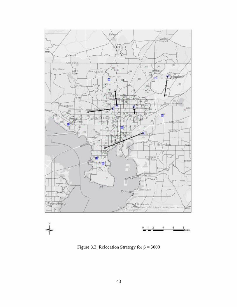
43
Figure 3.3: Relocation Strategy for β = 3000
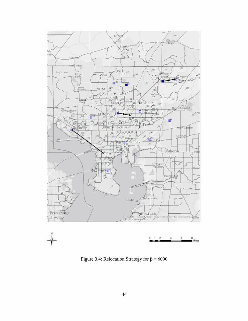
44
Figure 3.4: Relocation Strategy for β = 6000
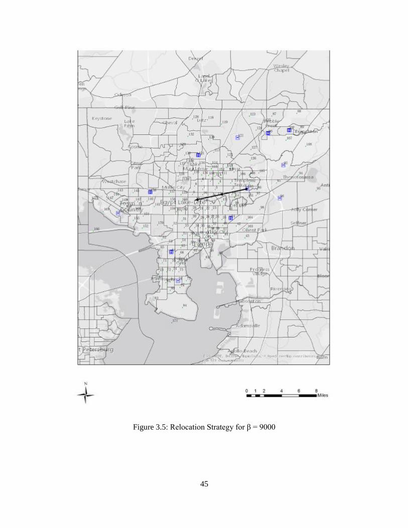
45
Figure 3.5: Relocation Strategy for β = 9000

46
Table 3.1: Computational Results of 𝑅𝑂_𝐸𝑀𝑆𝐿1 Model
|𝑾| 𝒑 𝒌 Time (s) Iter Obj Gap (%)
30 10 2 1.888 7 1190610
4 2.955 7 1158640
6 5.922 11 1123420
8 3.399 8 1088490
12 2 0.465 3 1088490
4 1.953 7 1181420
6 4.904 9 1151420
8 6.212 11 1112780
50 10 2 2.282 9 1191140
4 39.605 17 1157670
6 840.079 35 1119820
8 847.714 40 1089440
12 2 1.081 5 1207040
4 354.995 36 1165480
6 T 46 1120760 6.9
8 T 57 1080510 9.2

47
Table 3.2: Optimal Locations of 𝑅𝑂_𝐸𝑀𝑆𝐿1 Model
|𝑾| 𝒑 𝒌 𝒚∗
30 10 2 2 19 68 76 90 92 99 120 149 167
4 2 23 63 76 90 92 120 146 149 167
6 9 40 68 76 90 92 106 120 149 167
8 30 63 76 85 90 99 134 140 149 167
12 2 23 47 52 72 76 90 92 106 120 146 149 167
4 23 63 76 90 92 99 120 126 131 140 149 167
6 8 49 72 76 92 99 106 131 140 146 149 167
8 2 40 63 72 76 92 110 120 140 146 149 167
50 10 2 5 40 72 76 90 91 92 132 151 154
4 14 58 76 90 91 96 120 135 151 154
6 11 66 80 91 96 99 105 120 151 154
8 8 27 32 72 80 91 92 103 120 149
12 2 32 47 49 80 90 91 96 108 132 135 146
4 8 24 47 72 80 90 91 92 105 132 151 154
6 10 32 47 72 76 90 91 92 103 120 149 151
8 6 32 51 76 80 90 91 92 99 107 132 154

48
Table 3.3: Computational Results of 𝑅𝑂_𝐸𝑀𝑆𝐿2 Model
|𝑾| 𝒑 𝒌 Time (s) Iter Obj Gap (%)
30 10 2 0.049 3 1190820
4 8.184 6 1160610
6 83.413 11 1126910
8 259.63 15 1094680
12 2 0.596 2 1211460
4 2.288 4 1188950
6 9.814 6 1157500
8 207.23 14 1123960
50 10 2 0.708 2 1194020
4 127.063 7 1186730
6 2784.76 14 1158480
8 1229.72 11 1146710
12 2 0.634 2 1215140
4 2.817 4 1196870
6 272.072 8 1181330
8 T 23 1160160 5.6
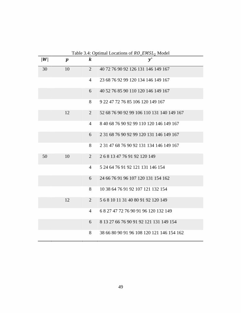
49
Table 3.4: Optimal Locations of 𝑅𝑂_𝐸𝑀𝑆𝐿2 Model
|𝑾| 𝒑 𝒌 𝒚∗
30 10 2 40 72 76 90 92 126 131 146 149 167
4 23 68 76 92 99 120 134 146 149 167
6 40 52 76 85 90 110 120 146 149 167
8 9 22 47 72 76 85 106 120 149 167
12 2 52 68 76 90 92 99 106 110 131 140 149 167
4 8 40 68 76 90 92 99 110 120 146 149 167
6 2 31 68 76 90 92 99 120 131 146 149 167
8 2 31 47 68 76 90 92 131 134 146 149 167
50 10 2 2 6 8 13 47 76 91 92 120 149
4 5 24 64 76 91 92 121 131 146 154
6 24 66 76 91 96 107 120 131 154 162
8 10 38 64 76 91 92 107 121 132 154
12 2 5 6 8 10 11 31 40 80 91 92 120 149
4 6 8 27 47 72 76 90 91 96 120 132 149
6 8 13 27 66 76 90 91 92 121 131 149 154
8 38 66 80 90 91 96 108 120 121 146 154 162

50
Table 3.5: Solution of Instance with p=12, k=6
𝒑 𝒌 𝜷 No. of Ambulances Need
Relocation
Optimal Relocation Strategies
From To From To
12 6 3000 5 13 1 66 165
90 90 92 91
131 6 146 8
6000 3 5 8 64 154
90 90 131 132
146 146 165 165
9000 1 19 103 76 76
92 92 96 96
121 121 154 154

51
CHAPTER 4: PESSIMISTIC OPTIMIZATION FOR VEHICLE SHARING PROGRAM
NETWORK DESIGN
4.1 Introduction
Vehicle sharing programs (VSPs) have gained its popularity rapidly in recent years. In
2010, there were an estimated 100 bicycle sharing programs in 125 cities worldwide with more
than 139,300 bicycles, and 45 were being planned in 22 nations [61]. Car sharing programs exist
in 600 cities, in 18 nations and on 4 continents [62]. The main factors for the growth of vehicle
sharing are the increasing congestion levels in urban cities; growing costs of personal vehicle
ownership; people’s mind change towards the ownership of cars. Unlike private vehicle, VSP
gives user the opportunity to utilize vehicle on demand. User can check out vehicles (bicycles,
cars) close to their origin and drop them off at VSP stations near their destinations. The cost of
utilizing such system is usually determined by the time of vehicle usage and mileage driven.
Some programs implemented an incentive mechanism that encourages user return vehicles to
designated VSP stations. The principle of shared-use vehicles is simple: users take advantage of
VSP to reduce their travel time and improve travel utility without worrying about the costs and
responsibilities of ownership. [63].
The VSP is an economic and sustainable urban transportation solution. VSP can either be
functioned as the individual modal which is independent of public transits, or as the extension of
the public transit network which provides the “last-mile” connections to the existing transit
services. For instance, for shorter trips, shared vehicles can be the sole transit modal from origin
52
to destination, while for longer trips, they can serve as the intermodal connect to existing transit
services so that users can take it as part of their travel itinerary. Therefore, the system network
design need to be carefully considered by the VSP operators. At system planning stage, VSP
operators determine the locations of the VSP stations, the number of slots and initial number of
shared-vehicles in each station. To exploit the potential of intermodalism, an optimal VSP
network design should be strongly collaborated with the existing transportation networks [64].
The VSP network design problem can be formulated as bi-level equilibrium network design
model. The model involves two stakeholders, VSP provider and user. On the upper level, VSP
provider (leader) determines the location of VSP stations, capacity and initial number of vehicles
in each station, while on the lower level, user (follower) react to the configuration by selecting
routes travel from origin to destination. VSP provider then adjusts the configuration in order to
achieve maximum utilization of the system. This leader-follower framework is essentially a
Stackelberg equilibrium, since the non-cooperative nature of the two stakeholders.
In this chapter, we study the pessimistic bi-level VSP network design problem which
receives no attention previously. We propose a pessimistic bi-level VSP network design model
and customized computational scheme. The model is tested on several prototypical transit
network instances. Experimental results show the significant differences between optimal
solutions in optimistic and pessimistic formulations. The remainder of this chapter is organized
as follows: in section 2, we review the existing literature on VSP network design; the pessimistic
VSP network design formulation and computational scheme are proposed in section 3; numerical
studies are conducted on various instances and results are presented in section 4; in section 5,
conclusions are made and future works are discussed.
53
4.2 Literature Review
The literature on VSP system design is growing in past years. Early studies were focused
on determining the feasibility of such novel systems [65], [66], potential of environment
consequences and effects on mobility behavior [67], [68], [69], [70].
From the operational perspective, some researchers study the operational characteristics
of vehicle sharing program. [71] developed a stochastic chance constrained mixed-integer
program to manage the fleet for vehicle sharing operations. The model incorporates a
probabilistic level of service constraint to ensure the redistribution plan must satisfy a proportion
of all demand scenarios. enumeration based technique and cone generation technique were
proposed for solving large systems. [72] proposed a model to estimate the capacity of bicycle
system and examine the viability of re-distribution of bicycles in the network to support more
flows. [73] developed a time-stepping simulation model to assess the efficiency of the different
relocation methods. More recent works seek optimal strategy for the fleet balancing and vehicles
repositioning. [74] proposed a variable neighborhood search with an embedded variable
neighborhood descent that exploits a series of neighborhood structures to generate candidate
routes for vehicles to visit unbalanced rental stations. [75] developed a mathematical
programming based 3-step heuristic to determine the routes for repositioning operations. The
proposed heuristic reduces the size of the routing problem by clustering together sets of points
that are likely to be visited consecutively. Routes among clusters are optimized and solution is
used to search for a good feasible route in the original network. [76] introduced a new planning
approach addressing both routing and assignment aspects of vehicle repositioning. Vehicle
routing model with sub tour elimination constraint and flow assignment model are developed.
[77] developed a proportional network flow based linear program to study optimal locations of
54
bike sharing docks and optimal bike allocations at each dock. Results show that the system
performance of the stochastic system could be approximated using deterministic linear
programing model.
While on the strategy design level, the VSP network design problem received very
limited attention. [78] presents an analytical hierarchy process (AHP) for car sharing stations
selection. The process ranks the stations by weights obtained from various criteria and experts’
on-hand experience, then select the stations whose total weights above a certain limit. [79]
presented an optimization approach to determine depot location, capacity considering relocation
of vehicles. The objective is to maximize daily profits considering revenues and operation costs.
Trip requests are known, three formulations with different types of service schemes are
proposed. [80] developed a comprehensive methodology for implementation, including the
estimation of potential demand and determining of optimal locations. [81] proposed a model
trading off the interests of both users and operators. However, the decisions of operators and
users are formed into a single objective function. This approach can be viewed as the system-
optimal utilization of the vehicle sharing resources. [82] developed a mixed-integer program
maximize the net revenue. User preferences are considered and estimated at zone level.
In practice, the objectives of users and VSP operators are often conflicting with each
other. Since VSP operators’ objective is to maximize the utilization of the system to gain profit,
however, user utilize the system only if it can reduce their travel disutility. To capture the
different objectives of two stakeholders, bi-level programming model was proposed by [64]. At
upper level, VSP operators (leader) first determine the optimal configuration of the system
(supply), users (follower) make corresponding response to the configuration by constructing
routes from origin to destination (demand). VSP operators then make adjustment to optimize
55
system utilization. They also proposed an exact solution approach to solve this problem.
However, the bi-level programming model is optimistic formulation. Users’ decision is based on
assumption that they are cooperative and always select routes in favor of the VSP operators’
interests. In practice, users are selfish and often behave non-cooperatively by taking solution
against VSP operators’ interest. The optimistic formulation is no longer sufficient to provide an
optimal solution, therefore pessimistic formulation (PBL) should be considered [83].
No previous work has studied the pessimistic aspect of the bi-level VSP network design
problem. This study filled the gap in the literature and contributions are provided in the
following. A novel pessimistic formulation of the bi-level VSP network design model and tight
relaxation for level reduction are proposed. A customized computational scheme is then
developed. The model is tested on several synthetic networks, comparisons of the solution to the
optimistic formulation are presented. Experimental results show by adopting pessimistic
formulation, the resulting optimal network configuration is significantly different from the one
from optimistic formulation. In fact, solutions obtained from pessimistic bi-level optimization
are more reliable and have the promising potential of identifying practical and robust VSP
network configurations.
4.3 Model and Evaluation
In this section, we first describe the optimistic formulation of the Bi-Level VSP network
design model (OBL-VSP), then we evaluate the reliability of the OBL-VSP and present a
pessimistic reformulation (PBL-VSP).
4.3.1 The Bi-level VSP Network Design Model
The vehicle-sharing network can be represented by a graph 𝐺(𝑉, 𝐴), where the set of
nodes 𝑉 including transit stations, candidate VSP stations and demand origins, destinations, the
56
set of arcs 𝐴 consist of transit links, sharing links, transfer links and walk links. Arcs connect
nodes in the graph 𝐺. A subset of arcs 𝐴 denoted by 𝐴𝐹 includes the frequency based arcs. Each
arc in 𝐴 is characterized by a pair (𝑐𝑖𝑗, 𝑔𝑖𝑗). Where 𝑐𝑖𝑗, 𝑔𝑖𝑗 denote the travel time (costs) and
waiting time of transit service respectively [84]. User travel through arcs (𝑖, 𝑗) with waiting
include a waiting time at node 𝑖 leading up to the frequency based arcs. And waiting time is
determined by the frequency of the transit services 𝑓𝑖𝑗 at terminal node 𝑗. The vehicle sharing
sub-network is denoted by 𝐺𝑠(𝑉𝑠, 𝐴𝑠) where 𝑉𝑠 are the candidate VSP stations and 𝐴𝑠 are the
shared vehicle links. For each arc in 𝐴𝑠, (𝑟𝑖𝑗, 𝑐𝑖𝑗) pair is used to denote the revenue to the VSP
operators and costs to the users.
At the upper level, vehicle sharing network configuration is denoted as 𝒙 by a 3-tuple
(𝑥, 𝑦, 𝑧). 𝑥𝑖 is binary decision variable determining whether to build VSP station at location 𝑖,
𝑖 ∈ 𝑉𝑠. 𝑦𝑖 represents the capacity of VSP station 𝑖, 𝑧𝑖 are the number of vehicles at 𝑖. 𝑐𝑠, 𝑐𝑝, 𝑐𝑣 are
setup costs, capacity expansion costs and unit vehicle costs respectively. The total cost denoted
by a scalar 𝐶. At the lower level, flow decision variables 𝑣𝑖𝑗𝑘 denotes the flows from node 𝑖 to 𝑗
of origin-destination pair 𝑘. 𝑤𝑖𝑘 represents the total waiting time in OD pair 𝑘 at node 𝑖. In
addition, the checkout replacement ratio is denoted by 𝑎, where 𝑎 = 1 means that capacity
satisfies checkouts and returns and 𝑎 > 1 otherwise.
The objective function for upper level is denoted by
𝐹(𝒗) = ∑ ∑ 𝑟𝑖𝑗𝑣𝑖𝑗𝑘
𝑖,𝑗∈𝐴𝑠𝑘
(52)
Objective function for lower level is denoted by
𝑓(𝒗, 𝒘) = ∑( ∑ 𝑐𝑖𝑗𝑣𝑖𝑗𝑘
(𝑖,𝑗)∈𝐴
+ ∑ 𝑤𝑖𝑘
𝑖∈𝑉
)
𝑘
(53)

57
Then the bi-level VSP network design model OBL-VSP can be written as:
max𝒗∈𝑆(𝒙,𝒚,𝒛)
𝐹(𝑣) (54)
s.t. ∑ 𝑐𝑠𝑥𝑖
𝑖∈𝑉𝑠
+ 𝑐𝑝𝑦𝑖 + 𝑐𝑣𝑧𝑖 ≤ 𝐶 (55)
𝑀𝑥𝑖 ≥ 𝑦𝑖 , ∀𝑖 ∈ 𝑉𝑠 (56)
𝑧𝑖 ≤ 𝑦𝑖, ∀𝑖 ∈ 𝑉𝑠 (57)
𝑦𝑖 ≤ 𝑦𝑢𝑏 , ∀𝑖 ∈ 𝑉𝑠 (58)
𝑥𝑖 ∈ {0,1}, ∀𝑖 ∈ 𝑉𝑠; 𝑦𝑖 , 𝑧𝑖 ∈ ℤ𝑛, ∀𝑖 ∈ 𝑉𝑠 (59)
𝑆(𝒙, 𝒚, 𝒛) = 𝑎𝑟𝑔𝑚𝑖𝑛𝒗,𝒘
{ 𝑓(𝒗, 𝒘): (60)
∑ 𝑣𝑖𝑗𝑘
𝑗:(𝑖,𝑗)∈𝐴
− ∑ 𝑣𝑗𝑖𝑘
𝑗:(𝑗,𝑖)∈𝐴
= 𝐷𝑖𝑘, ∀𝑖 ∈ 𝑉, 𝑘 ∈ 𝐾 (61)
𝑣𝑖𝑗𝑘 ≤ 𝑓𝑖𝑗𝑤𝑖𝑘, ∀(𝑖, 𝑗) ∈ 𝐴𝐹 , 𝑘 ∈ 𝐾 (62)
𝑀𝑥𝑖 ≥ ∑ 𝑣𝑖𝑗𝑘
𝑘
, ∀(𝑖, 𝑗) ∈ 𝐴𝑠 (63)
𝑀𝑥𝑗 ≥ ∑ 𝑣𝑖𝑗𝑘
𝑘
, ∀(𝑖, 𝑗) ∈ 𝐴𝑠 (64)
∑ ∑ 𝑣𝑖𝑗𝑘 ≤ 𝑧𝑖
𝑗:(𝑖,𝑗)∈𝐴𝑠𝑘
, ∀𝑖 ∈ 𝑉𝑠 (65)
∑ ∑ 𝑣𝑗𝑖𝑘
𝑗:(𝑗,𝑖)∈𝐴𝑠𝑘
≤ 𝑎(𝑦𝑖 − 𝑧𝑖), ∀𝑖 ∈ 𝑉𝑠 (66)
𝑤𝑖𝑘 ≥ 0, ∀𝑖 ∈ 𝑉, 𝑘 ∈ 𝐾; 𝑣𝑖𝑗𝑘 ≥ 0, ∀(𝑖, 𝑗) ∈ 𝐴, 𝑘 ∈ 𝐾} (67)
In this model, upper level program denotes VSP operator’s decision and determines the
optimal VSP configuration (𝑥, 𝑦, 𝑧) to maximize the revenue of shared-flows (54), subject to
costs and capacity constraints (55) – (59). The lower level problem represents user’s decision

58
and seeks to minimize total costs for a given upper level VSP network configuration. The lower
level problem involves a set of flow constraints (61) – (67) to determine the optimal flows for
user travel through the network from origin to destination.
In general, bi-level mixed-integer program typically has a non-convex feasible region
which results in difficulties in computation. This type of problems is recognized as NP-hard [85].
To address this challenge, various computational algorithms have been developed [86], [87].
When lower-level problem is convex, we can adopt Karush-Kuhn-Tucker (KKT) conditions and
replace the lower level problem by its KKT conditions. Therefore, the bi-level program becomes
a single level mathematical program with equilibrium constraints (MPEC) and can be readily
solved by existing MIP solvers.
For convenience, we represent the OBL-VSP using concise notation as follows:
𝑚𝑎𝑥𝒙∈𝑋
𝐹(𝒗)
s.t. 𝐺(𝒙, 𝒗) ≤ 0
𝑚𝑖𝑛𝒗∈𝑆
𝑓(𝒗) (68)
s.t. 𝑔(𝒙, 𝒗) ≤ 0
where 𝒙 = (𝑥, 𝑦, 𝑧) and 𝒗 = (𝑣, 𝑤) are the operator and user decision vectors respectively.
𝐺(𝒙, 𝒗) and 𝑔(𝒙, 𝒗) are the upper and lower level constraints sets.
4.3.2 Reliability of OBL-VSP Solution
Although OBL-VSP provides an effective approach for modeling the conflicting
objectives of VSP operators and users. However, it may be inefficient from user’s perspective
since user may not always follow operator’s decision. Hence solutions obtained from OBL-VSP
can be viewed as leader-optimal solutions. In fact, two critical factors have been neglected,
which may significantly affect the performance of OBL-VSP in practice:

59
1. For a given optimal configuration 𝒙∗, the lower-level solution may not be unique and
optimal to the user.
2. Given the non-unique lower-level solution, the user may not always select routes that
maximize revenue for the VSP operator.
Figure 4.1 illustrates the impact of those two factors using a small network instance. The
network has 4 VSP candidate station nodes (A, B, C, D) and one OD pair (O, D) with a flow of
10 units. The numbers for each shared-link and walk link represent the flow revenue and cost
respectively. Given the upper-level configuration B, D, figure on the left shows the optimal
lower-level solution to the upper-level objective, the resulting revenue and cost are both equal to
30 units. However, if user decides routes without considering revenue, the resulting solution to
the lower-level is shown on the right figure. In this situation, the corresponding revenue reduces
to 0 unit and cost remains at 30 units. Notice that, for two different flow decisions, the costs
remain the same while the revenues show a huge difference.
We then formulate a problem to evaluate the impact of those two factors on OBL-VSP.
We first solve OBL-VSP (68) and derive optimal configuration 𝒙∗, then for given 𝒙∗ we solve
lower-level program and obtain optimal value 𝑙∗. After that, we solve the following formulation
and get optimal value 𝑢∗. The comparison results are shown in section 4.4.
𝑚𝑖𝑛 𝐹(𝒙∗, 𝒗)
s.t. 𝑔(𝒙∗, 𝒗) ≤ 0 (69)
𝑓(𝒙∗, 𝒗) ≤ 𝑙∗
where 𝒙∗ = (𝒙∗, 𝒚∗, 𝒛∗), 𝒗 = (𝒗, 𝒘). Apparently, for a given 𝒙∗, (69) computes the performance
in pessimistic environment. As showed in the illustrative example, user may behave non-
cooperative and their decisions may not be in favor of operator’s interests. Hence, OBL-VSP

60
may not work in practice. To study this challenge, we introduce the pessimistic formulation in
the next section.
4.3.3 Pessimistic Bi-Level VSP Network Design Model
In the last subsection, we observe that regular OBL-VSP assume that users are always
cooperative by generating solutions to maximize VSP operator’s objective. However, users are in
fact selfish. When making the decision, they tend to overlook VSP operator’s interest and select
solutions that only minimize their travel costs. In many practical scenarios, those solutions are
against VSP operator’s interest. Therefore, we should consider the pessimistic bi-level
formulation for modeling and computing. We propose such pessimistic formulation PBL-VSP in
the following:
𝑚𝑖𝑛𝑥𝑖,𝑦𝑖,𝑧𝑖
𝑚𝑎𝑥(𝑣𝑖𝑗𝑘,𝑤𝑖𝑘)∈𝑆(𝑥𝑖,𝑦𝑖,𝑧𝑖)
−𝐹 (𝒗) (70)
s.t. ∑ 𝑐𝑠𝑥𝑖
𝑖∈𝑉𝑠
+ 𝑐𝑝𝑦𝑖 + 𝑐𝑣𝑧𝑖 ≤ 𝐶 (71)
𝑀𝑥𝑖 ≥ 𝑦𝑖 , ∀𝑖 ∈ 𝑉𝑠 (72)
𝑧𝑖 ≤ 𝑦𝑖, ∀𝑖 ∈ 𝑉𝑠 (73)
𝑦𝑖 ≤ 𝑦𝑢𝑏 , ∀𝑖 ∈ 𝑉𝑠 (74)
𝑥𝑖 ∈ {0,1}, ∀𝑖 ∈ 𝑉𝑠; 𝑦𝑖 , 𝑧𝑖 ∈ ℤ𝑛, ∀𝑖 ∈ 𝑉𝑠 (75)
(𝑣𝑖𝑗𝑘, 𝑤𝑖𝑘) ∈ 𝑆(𝑥𝑖, 𝑦𝑖, 𝑧𝑖) = 𝑎𝑟𝑔𝑚𝑖𝑛𝒗,𝒘
{ 𝑓(𝒗, 𝒘): (76)
∑ 𝑣𝑖𝑗𝑘
𝑗:(𝑖,𝑗)∈𝐴
− ∑ 𝑣𝑗𝑖𝑘
𝑗:(𝑗,𝑖)∈𝐴
= 𝐷𝑖𝑘, ∀𝑖 ∈ 𝑉, 𝑘 ∈ 𝐾 (77)
𝑣𝑖𝑗𝑘 ≤ 𝑓𝑖𝑗𝑤𝑖𝑘, ∀(𝑖, 𝑗) ∈ 𝐴𝐹 , 𝑘 ∈ 𝐾 (78)
𝑀𝑥𝑖 ≥ ∑ 𝑣𝑖𝑗𝑘
𝑘
, ∀(𝑖, 𝑗) ∈ 𝐴𝑠 (79)

61
𝑀𝑥𝑗 ≥ ∑ 𝑣𝑖𝑗𝑘
𝑘
, ∀(𝑖, 𝑗) ∈ 𝐴𝑠 (80)
∑ ∑ 𝑣𝑖𝑗𝑘 ≤ 𝑧𝑖
𝑗:(𝑖,𝑗)∈𝐴𝑠𝑘
, ∀𝑖 ∈ 𝑉𝑠 (81)
∑ ∑ 𝑣𝑗𝑖𝑘
𝑗:(𝑗,𝑖)∈𝐴𝑠𝑘
≤ 𝑎(𝑦𝑖 − 𝑧𝑖), ∀𝑖 ∈ 𝑉𝑠 (82)
𝑤𝑖𝑘 ≥ 0, ∀𝑖 ∈ 𝑉, 𝑘 ∈ 𝐾; 𝑣𝑖𝑗𝑘 ≥ 0, ∀(𝑖, 𝑗) ∈ 𝐴, 𝑘 ∈ 𝐾} (83)
Bi-level problem is typically very hard to solve, even the lower level problem is linear
program, it is NP-hard. The PBL-VSP is a three-level problem so that it is much more difficult
than the OBL-VSP in computation. However, a new computational scheme developed by [83] is
practically useful in solving pessimistic bi-level problems. By introducing a set of variables and
constraints that replicate those in the lower-level OBL-VSP, we obtain a tight relaxation RPBL-
VSP for PBL-VSP in the following:
𝑚𝑖𝑛𝑥𝑖,𝑦𝑖,𝑧𝑖,��𝑖𝑗𝑘,��𝑖𝑘
−𝐹(𝑣) (84)
s.t. ∑ 𝑐𝑠𝑥𝑖
𝑖∈𝑉𝑠
+ 𝑐𝑝𝑦𝑖 + 𝑐𝑣𝑧𝑖 ≤ 𝐶 (85)
𝑀𝑥𝑖 ≥ 𝑦𝑖 , ∀𝑖 ∈ 𝑉𝑠 (86)
𝑧𝑖 ≤ 𝑦𝑖, ∀𝑖 ∈ 𝑉𝑠 (87)
𝑦𝑖 ≤ 𝑦𝑢𝑏 , ∀𝑖 ∈ 𝑉𝑠 (88)
𝑥𝑖 ∈ {0,1}, ∀𝑖 ∈ 𝑉𝑠; 𝑦𝑖 , 𝑧𝑖 ∈ ℤ𝑛, ∀𝑖 ∈ 𝑉𝑠 (89)
∑ ��𝑖𝑗𝑘
𝑗:(𝑖,𝑗)∈𝐴
− ∑ ��𝑗𝑖𝑘
𝑗:(𝑗,𝑖)∈𝐴
= 𝐷𝑖𝑘, ∀𝑖 ∈ 𝑉, 𝑘 ∈ 𝐾 (90)
��𝑖𝑗𝑘 ≤ 𝑓𝑖𝑗��𝑖𝑘, ∀(𝑖, 𝑗) ∈ 𝐴𝐹 , 𝑘 ∈ 𝐾 (91)

62
𝑀𝑥𝑖 ≥ ∑ ��𝑖𝑗𝑘
𝑘
, ∀(𝑖, 𝑗) ∈ 𝐴𝑠 (92)
𝑀𝑥𝑗 ≥ ∑ ��𝑖𝑗𝑘
𝑘
, ∀(𝑖, 𝑗) ∈ 𝐴𝑠 (93)
∑ ∑ ��𝑖𝑗𝑘 ≤ 𝑧𝑖
𝑗:(𝑖,𝑗)∈𝐴𝑠𝑘
, ∀𝑖 ∈ 𝑉𝑠 (94)
∑ ∑ ��𝑗𝑖𝑘
𝑗:(𝑗,𝑖)∈𝐴𝑠𝑘
≤ 𝑎(𝑦𝑖 − 𝑧𝑖), ∀𝑖 ∈ 𝑉𝑠 (95)
��𝑖𝑘 ≥ 0, ∀𝑖 ∈ 𝑉, 𝑘 ∈ 𝐾; ��𝑖𝑗𝑘 ≥ 0, ∀(𝑖, 𝑗) ∈ 𝐴, 𝑘 ∈ 𝐾 (96)
(𝑣𝑖𝑗𝑘, 𝑤𝑖𝑘) ∈ 𝑎𝑟𝑔𝑚𝑖𝑛{ 𝐹(𝒗): (97)
∑ 𝑣𝑖𝑗𝑘
𝑗:(𝑖,𝑗)∈𝐴
− ∑ 𝑣𝑗𝑖𝑘
𝑗:(𝑗,𝑖)∈𝐴
= 𝐷𝑖𝑘, ∀𝑖 ∈ 𝑉, 𝑘 ∈ 𝐾 (98)
𝑣𝑖𝑗𝑘 ≤ 𝑓𝑖𝑗𝑤𝑖𝑘, ∀(𝑖, 𝑗) ∈ 𝐴𝐹 , 𝑘 ∈ 𝐾 (99)
𝑀𝑥𝑖 ≥ ∑ 𝑣𝑖𝑗𝑘
𝑘
, ∀(𝑖, 𝑗) ∈ 𝐴𝑠 (100)
𝑀𝑥𝑗 ≥ ∑ 𝑣𝑖𝑗𝑘
𝑘
, ∀(𝑖, 𝑗) ∈ 𝐴𝑠 (101)
∑ ∑ 𝑣𝑖𝑗𝑘 ≤ 𝑧𝑖
𝑗:(𝑖,𝑗)∈𝐴𝑠𝑘
, ∀𝑖 ∈ 𝑉𝑠 (102)
∑ ∑ 𝑣𝑗𝑖𝑘
𝑗:(𝑗,𝑖)∈𝐴𝑠𝑘
≤ 𝑎(𝑦𝑖 − 𝑧𝑖), ∀𝑖 ∈ 𝑉𝑠 (103)
𝑓(𝒗, 𝒘) ≤ 𝑓(��, ��) (104)
𝑤𝑖𝑘 ≥ 0, ∀𝑖 ∈ 𝑉, 𝑘 ∈ 𝐾; 𝑣𝑖𝑗𝑘 ≥ 0, ∀(𝑖, 𝑗) ∈ 𝐴, 𝑘 ∈ 𝐾} (105)
According to [83], constraint (104) ensures that 𝑣𝑖𝑗𝑘 , 𝑤𝑖𝑘 are an optimal solution of the
lower-level. Notice that, the lower-level problem of RPBL-VSP is still a convex program and we
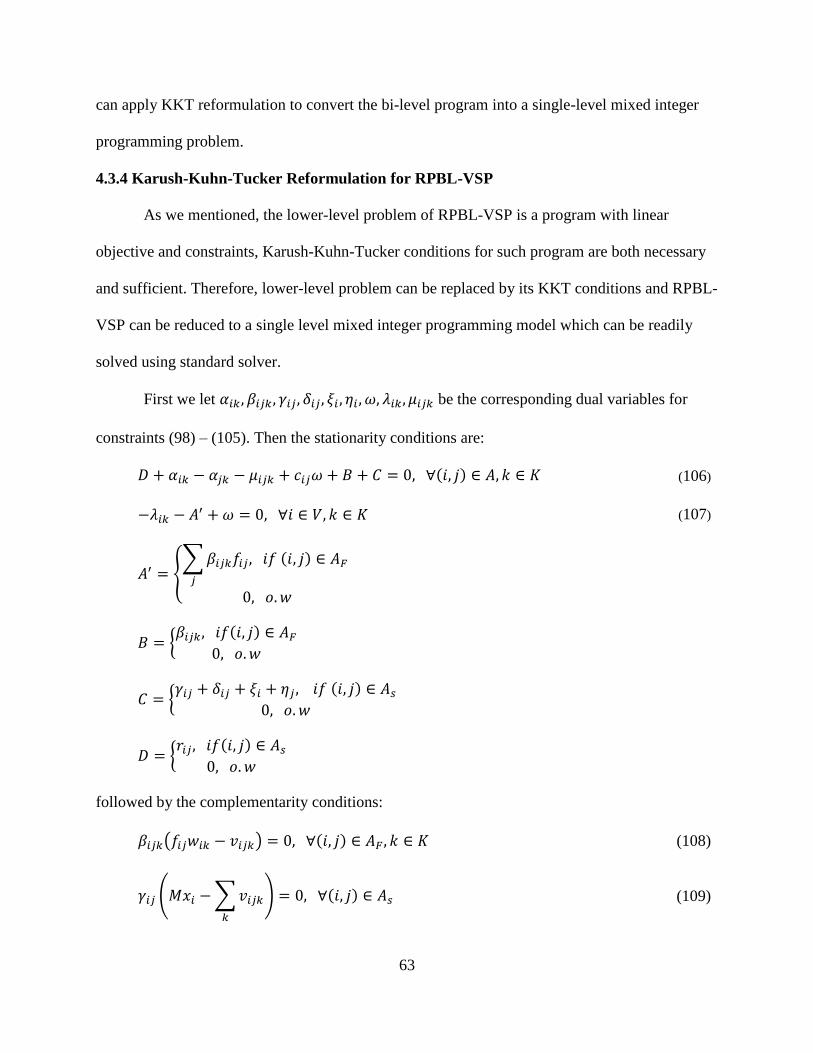
63
can apply KKT reformulation to convert the bi-level program into a single-level mixed integer
programming problem.
4.3.4 Karush-Kuhn-Tucker Reformulation for RPBL-VSP
As we mentioned, the lower-level problem of RPBL-VSP is a program with linear
objective and constraints, Karush-Kuhn-Tucker conditions for such program are both necessary
and sufficient. Therefore, lower-level problem can be replaced by its KKT conditions and RPBL-
VSP can be reduced to a single level mixed integer programming model which can be readily
solved using standard solver.
First we let 𝛼𝑖𝑘, 𝛽𝑖𝑗𝑘 , 𝛾𝑖𝑗, 𝛿𝑖𝑗, 𝜉𝑖 , 𝜂𝑖 , 𝜔, 𝜆𝑖𝑘, 𝜇𝑖𝑗𝑘 be the corresponding dual variables for
constraints (98) – (105). Then the stationarity conditions are:
𝐷 + 𝛼𝑖𝑘 − 𝛼𝑗𝑘 − 𝜇𝑖𝑗𝑘 + 𝑐𝑖𝑗𝜔 + 𝐵 + 𝐶 = 0, ∀(𝑖, 𝑗) ∈ 𝐴, 𝑘 ∈ 𝐾 (106)
−𝜆𝑖𝑘 − 𝐴′ + 𝜔 = 0, ∀𝑖 ∈ 𝑉, 𝑘 ∈ 𝐾 (107)
𝐴′ = {∑ 𝛽𝑖𝑗𝑘𝑓𝑖𝑗, 𝑖𝑓 (𝑖, 𝑗) ∈ 𝐴𝐹
𝑗
0, 𝑜. 𝑤
𝐵 = {𝛽𝑖𝑗𝑘, 𝑖𝑓(𝑖, 𝑗) ∈ 𝐴𝐹
0, 𝑜. 𝑤
𝐶 = {𝛾𝑖𝑗 + 𝛿𝑖𝑗 + 𝜉𝑖 + 𝜂𝑗 , 𝑖𝑓 (𝑖, 𝑗) ∈ 𝐴𝑠
0, 𝑜. 𝑤
𝐷 = {𝑟𝑖𝑗, 𝑖𝑓(𝑖, 𝑗) ∈ 𝐴𝑠
0, 𝑜. 𝑤
followed by the complementarity conditions:
𝛽𝑖𝑗𝑘(𝑓𝑖𝑗𝑤𝑖𝑘 − 𝑣𝑖𝑗𝑘) = 0, ∀(𝑖, 𝑗) ∈ 𝐴𝐹 , 𝑘 ∈ 𝐾 (108)
𝛾𝑖𝑗 (𝑀𝑥𝑖 − ∑ 𝑣𝑖𝑗𝑘
𝑘
) = 0, ∀(𝑖, 𝑗) ∈ 𝐴𝑠 (109)
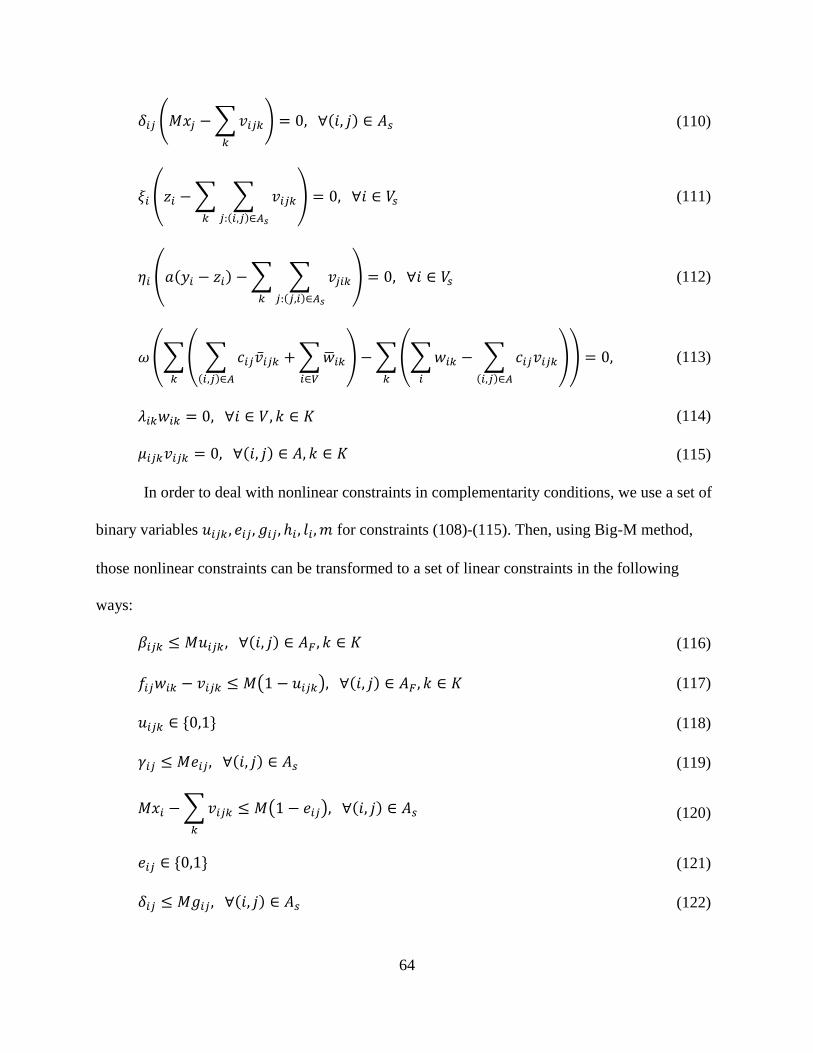
64
𝛿𝑖𝑗 (𝑀𝑥𝑗 − ∑ 𝑣𝑖𝑗𝑘
𝑘
) = 0, ∀(𝑖, 𝑗) ∈ 𝐴𝑠 (110)
𝜉𝑖 (𝑧𝑖 − ∑ ∑ 𝑣𝑖𝑗𝑘
𝑗:(𝑖,𝑗)∈𝐴𝑠𝑘
) = 0, ∀𝑖 ∈ 𝑉𝑠 (111)
𝜂𝑖 (𝑎(𝑦𝑖 − 𝑧𝑖) − ∑ ∑ 𝑣𝑗𝑖𝑘
𝑗:(𝑗,𝑖)∈𝐴𝑠𝑘
) = 0, ∀𝑖 ∈ 𝑉𝑠 (112)
𝜔 (∑ ( ∑ 𝑐𝑖𝑗��𝑖𝑗𝑘
(𝑖,𝑗)∈𝐴
+ ∑ ��𝑖𝑘
𝑖∈𝑉
)
𝑘
− ∑ (∑ 𝑤𝑖𝑘
𝑖
− ∑ 𝑐𝑖𝑗𝑣𝑖𝑗𝑘
(𝑖,𝑗)∈𝐴
)
𝑘
) = 0, (113)
𝜆𝑖𝑘𝑤𝑖𝑘 = 0, ∀𝑖 ∈ 𝑉, 𝑘 ∈ 𝐾 (114)
𝜇𝑖𝑗𝑘𝑣𝑖𝑗𝑘 = 0, ∀(𝑖, 𝑗) ∈ 𝐴, 𝑘 ∈ 𝐾 (115)
In order to deal with nonlinear constraints in complementarity conditions, we use a set of
binary variables 𝑢𝑖𝑗𝑘 , 𝑒𝑖𝑗, 𝑔𝑖𝑗, ℎ𝑖 , 𝑙𝑖, 𝑚 for constraints (108)-(115). Then, using Big-M method,
those nonlinear constraints can be transformed to a set of linear constraints in the following
ways:
𝛽𝑖𝑗𝑘 ≤ 𝑀𝑢𝑖𝑗𝑘 , ∀(𝑖, 𝑗) ∈ 𝐴𝐹 , 𝑘 ∈ 𝐾 (116)
𝑓𝑖𝑗𝑤𝑖𝑘 − 𝑣𝑖𝑗𝑘 ≤ 𝑀(1 − 𝑢𝑖𝑗𝑘), ∀(𝑖, 𝑗) ∈ 𝐴𝐹 , 𝑘 ∈ 𝐾 (117)
𝑢𝑖𝑗𝑘 ∈ {0,1} (118)
𝛾𝑖𝑗 ≤ 𝑀𝑒𝑖𝑗, ∀(𝑖, 𝑗) ∈ 𝐴𝑠 (119)
𝑀𝑥𝑖 − ∑ 𝑣𝑖𝑗𝑘
𝑘
≤ 𝑀(1 − 𝑒𝑖𝑗), ∀(𝑖, 𝑗) ∈ 𝐴𝑠 (120)
𝑒𝑖𝑗 ∈ {0,1} (121)
𝛿𝑖𝑗 ≤ 𝑀𝑔𝑖𝑗 , ∀(𝑖, 𝑗) ∈ 𝐴𝑠 (122)
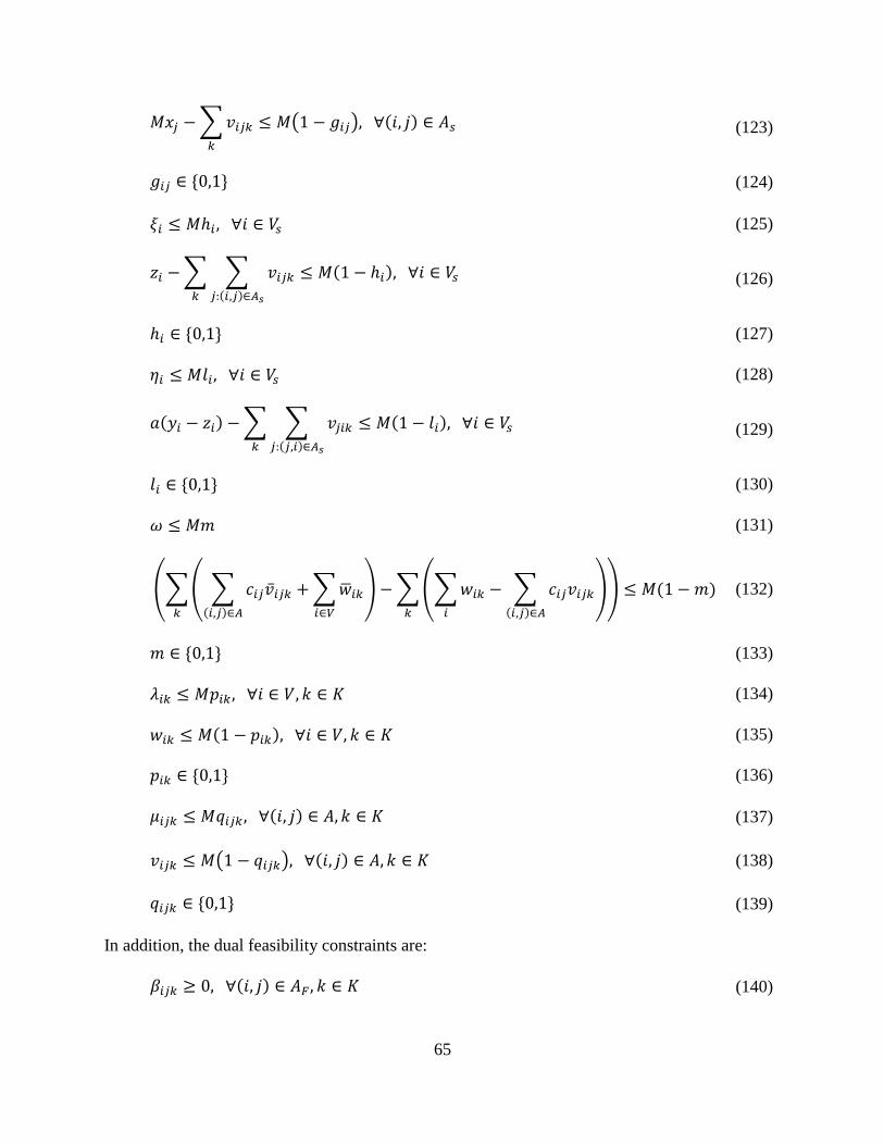
65
𝑀𝑥𝑗 − ∑ 𝑣𝑖𝑗𝑘
𝑘
≤ 𝑀(1 − 𝑔𝑖𝑗), ∀(𝑖, 𝑗) ∈ 𝐴𝑠 (123)
𝑔𝑖𝑗 ∈ {0,1} (124)
𝜉𝑖 ≤ 𝑀ℎ𝑖 , ∀𝑖 ∈ 𝑉𝑠 (125)
𝑧𝑖 − ∑ ∑ 𝑣𝑖𝑗𝑘
𝑗:(𝑖,𝑗)∈𝐴𝑠𝑘
≤ 𝑀(1 − ℎ𝑖), ∀𝑖 ∈ 𝑉𝑠 (126)
ℎ𝑖 ∈ {0,1} (127)
𝜂𝑖 ≤ 𝑀𝑙𝑖, ∀𝑖 ∈ 𝑉𝑠 (128)
𝑎(𝑦𝑖 − 𝑧𝑖) − ∑ ∑ 𝑣𝑗𝑖𝑘
𝑗:(𝑗,𝑖)∈𝐴𝑠𝑘
≤ 𝑀(1 − 𝑙𝑖), ∀𝑖 ∈ 𝑉𝑠 (129)
𝑙𝑖 ∈ {0,1} (130)
𝜔 ≤ 𝑀𝑚 (131)
(∑ ( ∑ 𝑐𝑖𝑗��𝑖𝑗𝑘
(𝑖,𝑗)∈𝐴
+ ∑ ��𝑖𝑘
𝑖∈𝑉
)
𝑘
− ∑ (∑ 𝑤𝑖𝑘
𝑖
− ∑ 𝑐𝑖𝑗𝑣𝑖𝑗𝑘
(𝑖,𝑗)∈𝐴
)
𝑘
) ≤ 𝑀(1 − 𝑚) (132)
𝑚 ∈ {0,1} (133)
𝜆𝑖𝑘 ≤ 𝑀𝑝𝑖𝑘, ∀𝑖 ∈ 𝑉, 𝑘 ∈ 𝐾 (134)
𝑤𝑖𝑘 ≤ 𝑀(1 − 𝑝𝑖𝑘), ∀𝑖 ∈ 𝑉, 𝑘 ∈ 𝐾 (135)
𝑝𝑖𝑘 ∈ {0,1} (136)
𝜇𝑖𝑗𝑘 ≤ 𝑀𝑞𝑖𝑗𝑘, ∀(𝑖, 𝑗) ∈ 𝐴, 𝑘 ∈ 𝐾 (137)
𝑣𝑖𝑗𝑘 ≤ 𝑀(1 − 𝑞𝑖𝑗𝑘), ∀(𝑖, 𝑗) ∈ 𝐴, 𝑘 ∈ 𝐾 (138)
𝑞𝑖𝑗𝑘 ∈ {0,1} (139)
In addition, the dual feasibility constraints are:
𝛽𝑖𝑗𝑘 ≥ 0, ∀(𝑖, 𝑗) ∈ 𝐴𝐹 , 𝑘 ∈ 𝐾 (140)
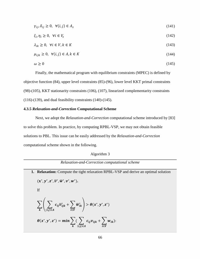
66
𝛾𝑖𝑗, 𝛿𝑖𝑗 ≥ 0, ∀(𝑖, 𝑗) ∈ 𝐴𝑠 (141)
𝜉𝑖, 𝜂𝑖 ≥ 0, ∀𝑖 ∈ 𝑉𝑠 (142)
𝜆𝑖𝑘 ≥ 0, ∀𝑖 ∈ 𝑉, 𝑘 ∈ 𝐾 (143)
𝜇𝑖𝑗𝑘 ≥ 0, ∀(𝑖, 𝑗) ∈ 𝐴, 𝑘 ∈ 𝐾 (144)
𝜔 ≥ 0 (145)
Finally, the mathematical program with equilibrium constraints (MPEC) is defined by
objective function (84), upper level constraints (85)-(96), lower level KKT primal constraints
(98)-(105), KKT stationarity constraints (106), (107), linearized complementarity constraints
(116)-(139), and dual feasibility constraints (140)-(145).
4.3.5 Relaxation-and-Correction Computational Scheme
Next, we adopt the Relaxation-and-Correction computational scheme introduced by [83]
to solve this problem. In practice, by computing RPBL-VSP, we may not obtain feasible
solutions to PBL. This issue can be easily addressed by the Relaxation-and-Correction
computational scheme shown in the following.
Algorithm 3
Relaxation-and-Correction computational scheme
1. Relaxation: Compute the tight relaxation RPBL-VSP and derive an optimal solution
(𝐱∗, 𝒚∗, 𝒛∗, ��∗, ��∗, 𝒗∗, 𝒘∗).
If
∑ ( ∑ 𝒄𝒊𝒋��𝒊𝒋𝒌∗
(𝒊,𝒋)∈𝑨
+ ∑ ��𝒊𝒌∗
𝒊∈𝑽
)
𝒌
> 𝜽(𝒙∗, 𝒚∗, 𝒛∗)
𝜽(𝒙∗, 𝒚∗, 𝒛∗) = 𝒎𝒊𝒏 ∑( ∑ 𝒄𝒊𝒋𝒗𝒊𝒋𝒌
(𝒊,𝒋)∈𝑨
+ ∑ 𝒘𝒊𝒌
𝒊∈𝑽
)
𝒌
:
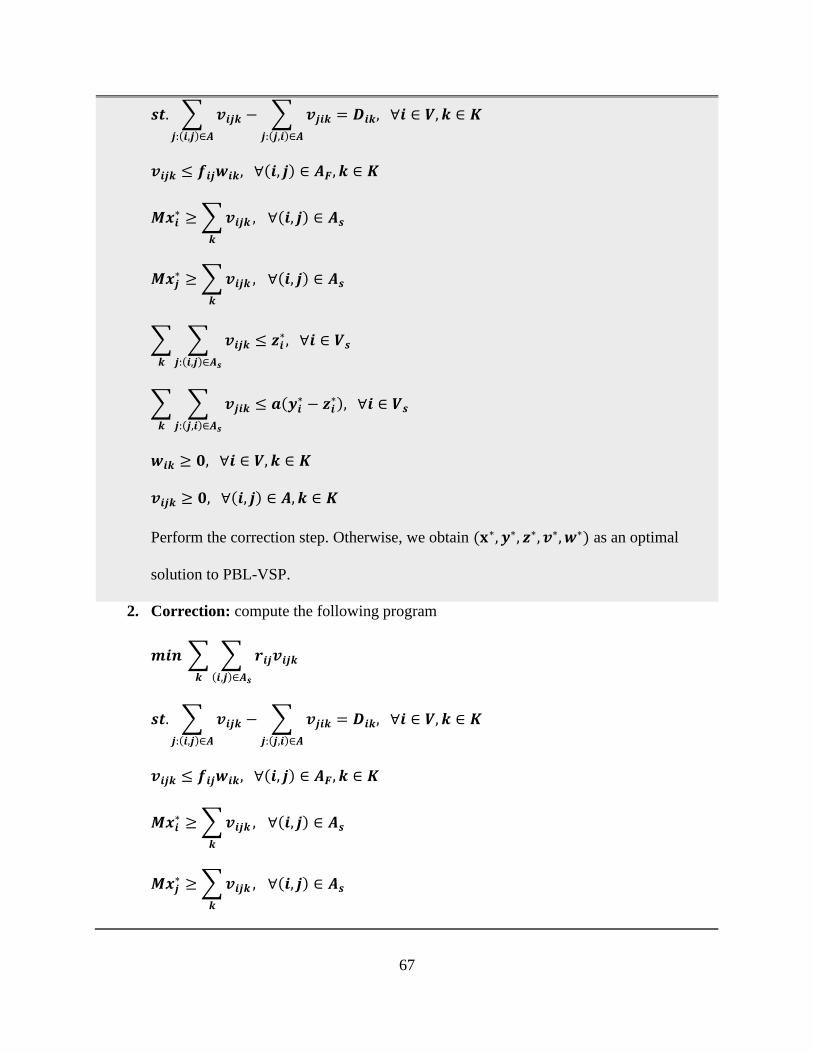
67
𝒔𝒕. ∑ 𝒗𝒊𝒋𝒌
𝒋:(𝒊,𝒋)∈𝑨
− ∑ 𝒗𝒋𝒊𝒌
𝒋:(𝒋,𝒊)∈𝑨
= 𝑫𝒊𝒌, ∀𝒊 ∈ 𝑽, 𝒌 ∈ 𝑲
𝒗𝒊𝒋𝒌 ≤ 𝒇𝒊𝒋𝒘𝒊𝒌, ∀(𝒊, 𝒋) ∈ 𝑨𝑭, 𝒌 ∈ 𝑲
𝑴𝒙𝒊∗ ≥ ∑ 𝒗𝒊𝒋𝒌
𝒌
, ∀(𝒊, 𝒋) ∈ 𝑨𝒔
𝑴𝒙𝒋∗ ≥ ∑ 𝒗𝒊𝒋𝒌
𝒌
, ∀(𝒊, 𝒋) ∈ 𝑨𝒔
∑ ∑ 𝒗𝒊𝒋𝒌
𝒋:(𝒊,𝒋)∈𝑨𝒔𝒌
≤ 𝒛𝒊∗, ∀𝒊 ∈ 𝑽𝒔
∑ ∑ 𝒗𝒋𝒊𝒌
𝒋:(𝒋,𝒊)∈𝑨𝒔𝒌
≤ 𝒂(𝒚𝒊∗ − 𝒛𝒊
∗), ∀𝒊 ∈ 𝑽𝒔
𝒘𝒊𝒌 ≥ 𝟎, ∀𝒊 ∈ 𝑽, 𝒌 ∈ 𝑲
𝒗𝒊𝒋𝒌 ≥ 𝟎, ∀(𝒊, 𝒋) ∈ 𝑨, 𝒌 ∈ 𝑲
Perform the correction step. Otherwise, we obtain (𝐱∗, 𝒚∗, 𝒛∗, 𝒗∗, 𝒘∗) as an optimal
solution to PBL-VSP.
2. Correction: compute the following program
𝒎𝒊𝒏 ∑ ∑ 𝒓𝒊𝒋𝒗𝒊𝒋𝒌
(𝒊,𝒋)∈𝑨𝒔𝒌
𝒔𝒕. ∑ 𝒗𝒊𝒋𝒌
𝒋:(𝒊,𝒋)∈𝑨
− ∑ 𝒗𝒋𝒊𝒌
𝒋:(𝒋,𝒊)∈𝑨
= 𝑫𝒊𝒌, ∀𝒊 ∈ 𝑽, 𝒌 ∈ 𝑲
𝒗𝒊𝒋𝒌 ≤ 𝒇𝒊𝒋𝒘𝒊𝒌, ∀(𝒊, 𝒋) ∈ 𝑨𝑭, 𝒌 ∈ 𝑲
𝑴𝒙𝒊∗ ≥ ∑ 𝒗𝒊𝒋𝒌
𝒌
, ∀(𝒊, 𝒋) ∈ 𝑨𝒔
𝑴𝒙𝒋∗ ≥ ∑ 𝒗𝒊𝒋𝒌
𝒌
, ∀(𝒊, 𝒋) ∈ 𝑨𝒔

68
∑ ∑ 𝒗𝒊𝒋𝒌
𝒋:(𝒊,𝒋)∈𝑨𝒔𝒌
≤ 𝒛𝒊∗, ∀𝒊 ∈ 𝑽𝒔
∑ ∑ 𝒗𝒋𝒊𝒌
𝒋:(𝒋,𝒊)∈𝑨𝒔𝒌
≤ 𝒂(𝒚𝒊∗ − 𝒛𝒊
∗), ∀𝒊 ∈ 𝑽𝒔
𝒘𝒊𝒌 ≥ 𝟎, ∀𝒊 ∈ 𝑽, 𝒌 ∈ 𝑲
𝒗𝒊𝒋𝒌 ≥ 𝟎, ∀(𝒊, 𝒋) ∈ 𝑨, 𝒌 ∈ 𝑲
∑( ∑ 𝒄𝒊𝒋𝒗𝒊𝒋𝒌
(𝒊,𝒋)∈𝑨
+ ∑ 𝒘𝒊𝒌
𝒊∈𝑽
)
𝒌
≤ 𝜽(𝒙∗, 𝒚∗, 𝒛∗)
Derive an optimal solution (𝒗′, 𝒘′). Optimal solution (𝐱∗, 𝒚∗, 𝒛∗, 𝒗′, 𝒘′) is obtained.
4.4 Numerical Experiment
In this section, the key objective is to examine the efficiency of pessimistic formulation
and solution method, study the effect of input parameters and different network characteristics,
compare the performance and differences between pessimistic and optimistic formulations in
regard of the solutions and provide management insights in designing a reliable VSP network.
First, we demonstrate the results using the illustrative example to gain initial insights on
the solutions. Then, we conduct experiments on various instances with different network
structures followed by discussion.
Figure 4.2 shows the results obtained by solving OBL-VSP and PBL-VSP. In optimistic
solution, VSP stations B and D are built and corresponding user’s flow is O-B-D. The resulting
revenue and cost are both 30 units. Nevertheless, in pessimistic solution, VSP stations A and D
are built with route decision O-A-D, the revenue and cost associated with this design are 20 units
and 10 units. If VSP operator build stations based on OBL-VSP solution, user’s non-cooperative
behavior will lead to 0 unit revenue to the VSP operator.
69
In the experiments, three types of network structures are considered, shown in Figure 4.3,
Figure 4.4, Figure 4.5, with circles represent transit stations, squares denote candidate VSP
stations and the black lines represent transit services. Figure 4.3 shows the corridor network
(COR), in this network, transit services run along a corridor with shared-vehicles providing
access to transit stations. Figure 4.4 shows the grid network (GRID) which mimic the transit
services in the downtown area, shared-vehicles provide additional intermodal path choices to the
users. Figure 4.5 denotes the random network (RND), where the nodes and arcs are randomly
generated. For each network structure, we generated several instances denoted by the network
type (e.g. COR) and the number of node (e.g. COR23). Table 4.1 shows the summary of each
instance. We observe that, for the same instance, the numbers of integer variables in PBL-VSP
and OBL-VSP are nearly identical, while the number of continuous variables in PBL-VSP are
larger since a set of new variables and constraints that replicate the lower level program were
added.
Nodes are categorized by transit stations, VSP candidate stations, and
origins/destinations. Links are classified into three types, walk links, shared-vehicle links, and
transit links. For walk links, we assume a constant walking speed of 5 miles/hour. And 30
miles/hour for shared-vehicle links and transit links. Parameter Budget is varied from 0 – 100
with the increment of 20 for each instance. The parameters of cost components 𝑐𝑠, 𝑐𝑝, 𝑐𝑣 are set
to 4,2,1 respectively. Solution time limit set to one hour. The models and computational scheme
are implemented in C++, solved by CPLEX 12.5 solver. Table 4.2 shows the computational
results. The upper and lower level objective values of PBL-VSP and OBL-VSP as well as
solution time in seconds are also reported. For instances that solution time exceeds limit, we
report the MIP gap (%). The values in column OBL-P denotes that OBL performance in
70
pessimistic environment as we discussed in section 4.3.2. From the experiments, we notice that
solution time increases with respect to the number of nodes and budget. Due to the combinatorial
nature of this problem, networks with more than 40 nodes and budget greater than 100 require
huge amount of time (>10 hours) for CPLEX to find solution with relatively large gaps. To
benchmark the optimal network configurations, we omit those instances and only include
instances that can be solved to optimality within time limit.
Figure 4.6 and Figure 4.8 present the VSP operator’s revenue and user’s cost as a
function of budget in PBL-VSP. Figure 4.7 and Figure 4.9 show the same information in OBL-
VSP. It can be seen from those figures that VSP operator’s revenue is slightly higher in OBL-
VSP than in PBL-VSP among tested instances, while lower level user cost in PBL-VSP is lower
than that in OBL-VSP. To better understand the results, we plot upper level objective values in
PBL-VSP, OBL-VSP and OBL-P, lower level objective values in PBL-VSP and OBL-VSP with
respect to budget for each instance, see Figure 4.10 -Figure 4.18. Results show that OBL-VSP
has highest upper and lower level optimal values since users make corresponding route decisions
to maximize VSP operator’s revenue while sacrificing their travel utility if the cooperative
assumption holds. OBL-P solutions are the least favorable solutions to VSP operators if users
behave non-cooperative and seek solutions only to minimize their costs regardless of VSP
operator’s interest. For example, in instance COR32, when C=80, PBL-VSP solution yields 36
units of revenue comparing to 58 units in OBL-VSP solution. However, the corresponding costs
for users in PBL-VSP equal to 519.667 which is lower than 526.667 in OBL-VSP. In non-
cooperative situation, OBL-VSP solution only results in 8 units of revenue. This result shows
that if users behave non-cooperatively, VSP operator can only gain 8 units of revenue from the
optimal OBL-VSP configuration. Comparing to the expected revenue of 58 units, the result is
71
less desirable and therefore we can conclude that OBL-VSP cannot provide optimal network
configuration in practice.
Furthermore, the networks derived from PBL-VSP and OBL-VSP for instance RND 34
are presented in Figure 4.19 - Figure 4.29 with budget C varies from 0-100. The detailed optimal
capacities and number of vehicles in each station are shown in Table 4.3. When budget C is in
the range of 0-100, the budget constraint is binding, hence only a subset of the VSP candidate
stations will be selected to build. It is obvious that the network configuration obtained from PBL-
VSP and OBL-VSP are different with the increase of budget. When C=100, we observe that for a
same origin-destination pair, user select route segments with lower costs in PBL-VSP than that
in OBL-VSP, as the result, lower level optimal value 𝑓(𝑣) in PBL-VSP is 785 which is less than
853 in OBL-VSP. On the contrary, route segments with higher revenue are chosen in OBL-VSP,
the resulting upper level optimal value 𝐹(𝑣) is 54 in OBL-VSP and 30 in PBL-VSP. The results
show that in OBL-VSP, user make decisions to incorporate with VSP operator’s interest. The
network configuration is optimal to VSP operator, however, it is suboptimal to user and lead to
larger travel costs. By computing OBL-P, we obtain the upper level objective value 𝐹(𝑣) =21,
which represents the OBL-VSP configuration in pessimistic environment if the non-cooperative
assumption holds. Since VSP operator cannot control over the user’s behavior, solution obtained
from OBL-VSP could give arbitrarily low revenue if cooperative assumption is not effective.
Clearly, PBL-VSP will derive robust and reliable network design when dealing with the users’
irrationality.
4.5 Conclusion and Future Work
In this study, we examine the reliability issue raised from the optimistic bi-level
equilibrium design of the vehicle sharing program (OBL-VSP). The equilibrium solution is

72
inefficient since two stakeholders do not cooperate and could get arbitrarily low revenue. To
address this issue, a pessimistic formulation (PBL-VSP) is proposed. A tight relaxation is
developed for level reduction and a Relaxation-and-Correction computational scheme is
implemented for solving the problem. We conduct experiments on several random prototypical
networks with different structures to show the capability of the model and benchmark results
with optimistic formulation. Results show PBL-VSP is more efficient in designing a reliable and
robust VSP network.
The future work of this study could be extended to adopt more realistic origin-destination
estimation method and incorporate congestion effects on the networks to obtain additional
insights. Furthermore, other solution algorithms and decomposition methods could be explored
to deal with large-scale instances in practice.
Figure 4.1: Illustrative Example
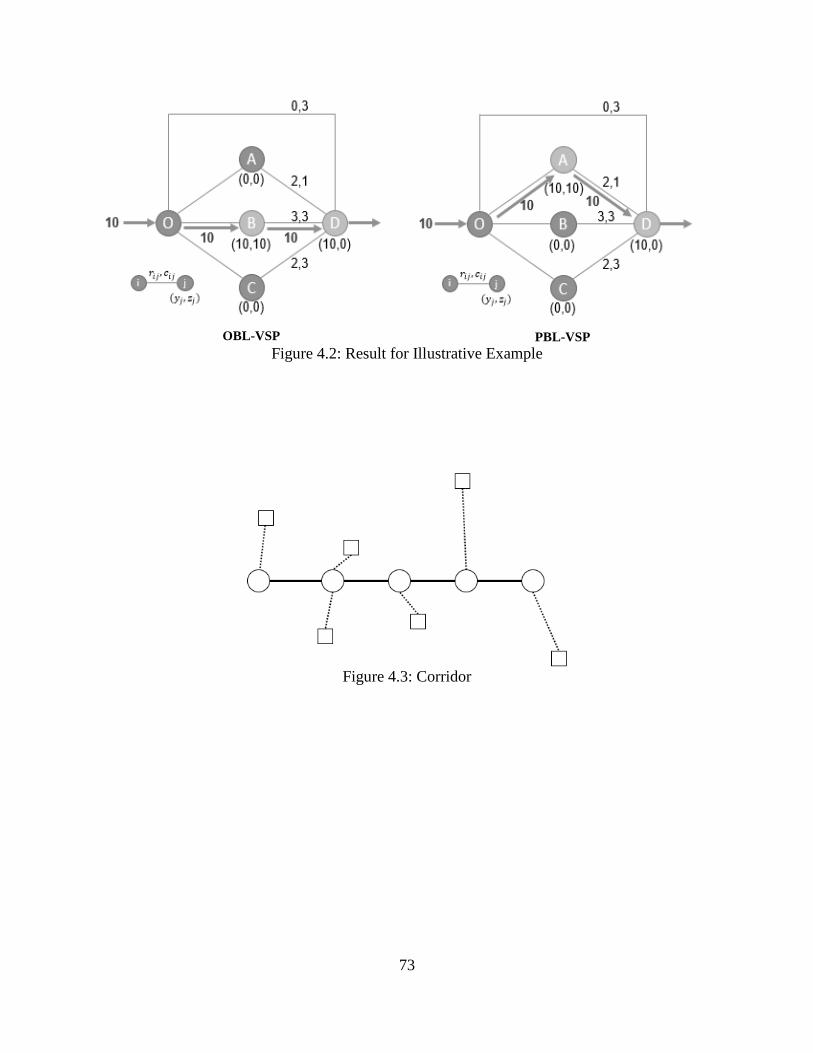
73
OBL-VSP
PBL-VSP
Figure 4.2: Result for Illustrative Example
Figure 4.3: Corridor
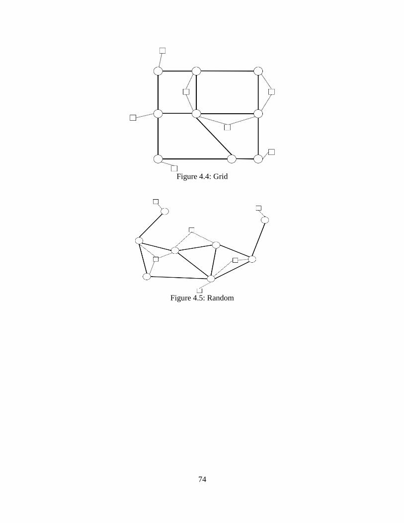
74
Figure 4.4: Grid
Figure 4.5: Random
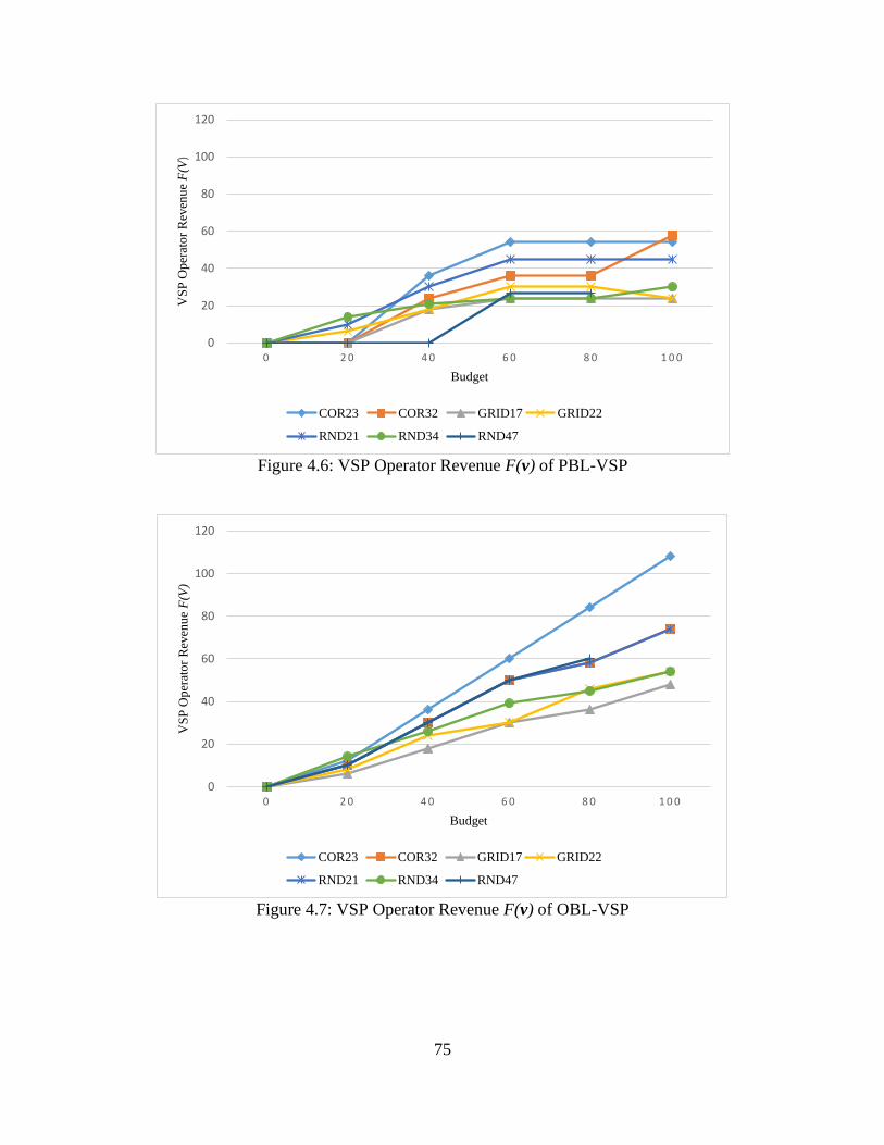
75
Figure 4.6: VSP Operator Revenue F(v) of PBL-VSP
Figure 4.7: VSP Operator Revenue F(v) of OBL-VSP
0
20
40
60
80
100
120
0 20 40 60 80 100
VS
P O
per
ato
r R
even
ue
F(V)
Budget
COR23 COR32 GRID17 GRID22
RND21 RND34 RND47
0
20
40
60
80
100
120
0 20 40 60 80 100
VS
P O
per
ato
r R
even
ue
F(V
)
Budget
COR23 COR32 GRID17 GRID22
RND21 RND34 RND47
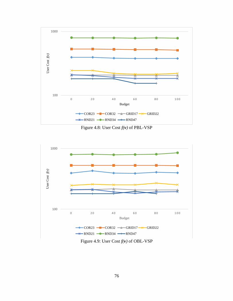
76
Figure 4.8: User Cost f(v) of PBL-VSP
Figure 4.9: User Cost f(v) of OBL-VSP
100
1000
0 20 40 60 80 100
Use
r C
ost
f(
v)
Budget
COR23 COR32 GRID17 GRID22
RND21 RND34 RND47
100
1000
0 20 40 60 80 100
Use
r C
ost
f(
v)
Budget
COR23 COR32 GRID17 GRID22
RND21 RND34 RND47

77
𝑭(𝒗)
𝒇(𝒗)
Figure 4.10: COR 23
𝑭(𝒗)
𝒇(𝒗)
Figure 4.11: COR 32
0
20
40
60
80
100
120
0 2 0 4 0 6 0 8 0 1 0 0
PBL OBL OBL-P
350
360
370
380
390
400
410
420
430
440
0 2 0 4 0 6 0 8 0 1 0 0
PBL OBL
0
10
20
30
40
50
60
70
80
0 2 0 4 0 6 0 8 0 1 0 0
PBL OBL OBL-P
495
500
505
510
515
520
525
530
535
0 2 0 4 0 6 0 8 0 1 0 0
PBL OBL

78
𝑭(𝒗)
𝒇(𝒗)
Figure 4.12: GRID 17
𝑭(𝒗)
𝒇(𝒗)
Figure 4.13: GRID 22
0
10
20
30
40
50
60
0 2 0 4 0 6 0 8 0 1 0 0
PBL OBL OBL-P
200
202
204
206
208
210
212
214
216
218
0 2 0 4 0 6 0 8 0 1 0 0
PBL OBL
0
10
20
30
40
50
60
0 2 0 4 0 6 0 8 0 1 0 0
PBL OBL OBL-P
0
50
100
150
200
250
300
0 2 0 4 0 6 0 8 0 1 0 0
PBL OBL

79
𝑭(𝒗)
𝒇(𝒗)
Figure 4.14: RND 21
𝑭(𝒗)
𝒇(𝒗)
Figure 4.15: RND 34
0
10
20
30
40
50
60
70
80
0 20 40 60 80 100
PBL OBL OBL-P
165
170
175
180
185
190
195
200
205
210
215
0 20 40 60 80 100
PBL OBL
0
10
20
30
40
50
60
0 2 0 4 0 6 0 8 0 1 0 0
PBL OBL OBL-P
740
760
780
800
820
840
860
0 2 0 4 0 6 0 8 0 1 0 0
PBL OBL
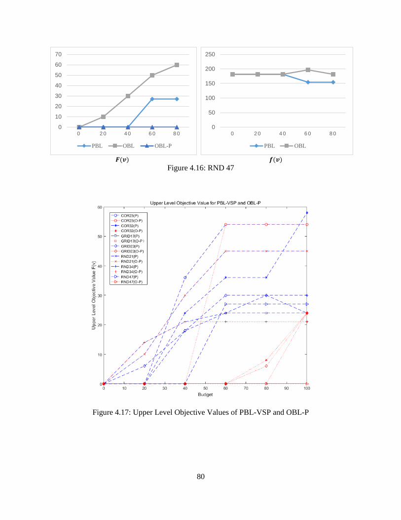
80
𝑭(𝒗)
𝒇(𝒗)
Figure 4.16: RND 47
Figure 4.17: Upper Level Objective Values of PBL-VSP and OBL-P
0
10
20
30
40
50
60
70
0 2 0 4 0 6 0 8 0
PBL OBL OBL-P
0
50
100
150
200
250
0 2 0 4 0 6 0 8 0
PBL OBL
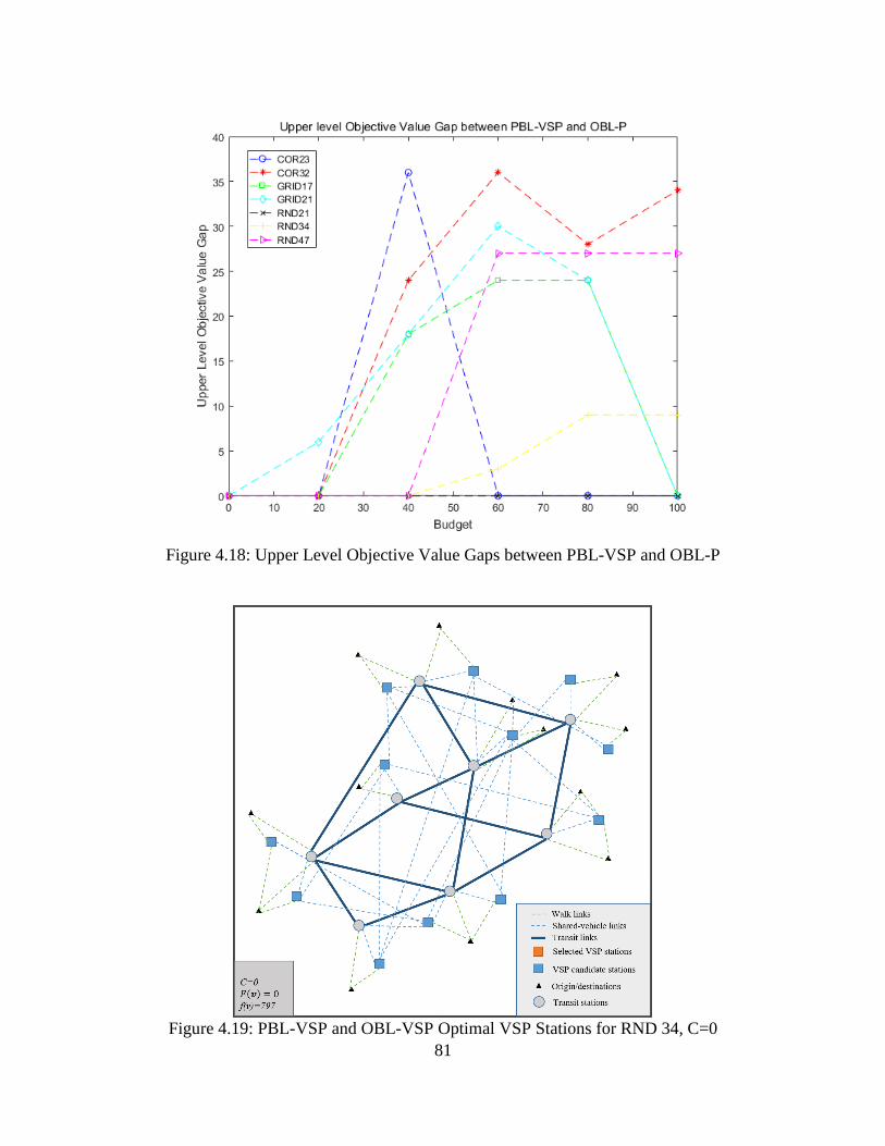
81
Figure 4.18: Upper Level Objective Value Gaps between PBL-VSP and OBL-P
Figure 4.19: PBL-VSP and OBL-VSP Optimal VSP Stations for RND 34, C=0

82
Figure 4.20: PBL-VSP Optimal VSP Stations for RND 34, C=20
Figure 4.21: OBL-VSP Optimal VSP Stations for RND 34, C=20
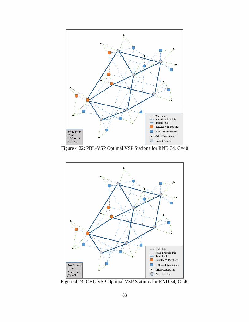
83
Figure 4.22: PBL-VSP Optimal VSP Stations for RND 34, C=40
Figure 4.23: OBL-VSP Optimal VSP Stations for RND 34, C=40

84
Figure 4.24: PBL-VSP Optimal VSP Stations for RND 34, C=60
Figure 4.25: OBL-VSP Optimal VSP Stations for RND 34, C=60

85
Figure 4.26: PBL-VSP Optimal VSP Stations for RND 34, C=80
Figure 4.27: OBL-VSP Optimal VSP Stations for RND 34, C=80

86
Figure 4.28: PBL-VSP Optimal VSP Stations for RND 34, C=100
Figure 4.29: OBL-VSP Optimal VSP Stations for RND 34, C=100

87
Table 4.1: Summary of Network Instances
Network Instance Nodes Links Transit
Services
VSP
sites
PBL OBL
Int.vars Cont.vars Int.vars Cont.vars
Corridor COR23 23 74 2 7 497 1237 496 940
COR32 32 102 4 11 684 1850 683 1314
GRID GRID17 17 56 3 11 331 786 330 567
GRID21 21 69 3 8 452 1129 451 889
RND RND21 21 72 3 7 577 1284 576 912
RND34 34 118 5 12 1509 2761 1508 1704
RND47 47 164 6 19 1558 3049 1557 1783
Table 4.2: Computational Results
Instance Budget PBL OBL OBL-
P
𝐹(𝑣) f(v) Time 𝐹(𝑣) f(v) Time 𝐹(𝑣)
COR23 0 0 394.667 0.454 0 394
.66
7
0.189 0
20 0 394.667 2.47 12 429
.66
6
0.377 0
40 36 382.667 1.874 36 394
.66
7
0.418 0
60 54 376.667 74.798 60 388
.66
7
50.594 54
80 54 376.667 53.347 84 406
.66
7
20.457 54
100 54 376.667 40.272 108 396
.66
7
30.73 54
COR32 0 0 528.667 0.671 0 528
.66
7
0.205 0
20 0 528.667 1.165 10 528
.66
7
0.323 0
40 24 522.667 71.575 30 528
.66
7
50.323 0
60 36 519.667 13.289 50 528
.66
7
10.286 0
80 36 519.667 87.97 58 526
.66
7
60.632 8

88
Table 4.2: (Continued)
100 58 506.667 98.97 74 522.667 54.33 24
GRID17 0 0 208.333 0.256 0 208.333 0.203 0
20 0 208.333 0.527 6 209.476 0.405 0
40 18 206.333 2.549 18 216.250 0.393 0
60 24 205.667 50.57 30 208.333 10.286 0
80 24 205.667 81.117 36 208.333 62.661 0
100 24 205.667 189.921 48 208.333 110.736 24
GRID22 0 0 244.5 0.15 0 246.283 0.254 0
20 6 244 3.887 8 257.923 0.636 0
40 18 220.5 44.237 24 252.067 23.385 0
60 30 214.5 38.226 30 250.885 26.385 0
80 30 214.5 183.152 46 267.924 89.357 6
100 24 220.5 263.094 54 253.4 235.281 24
RND21 0 0 210 0.411 0 210 0.086 0
20 10 204 0.509 10 212 0.218 10
40 30 192 3.999 30 192 0.211 30
60 45 183 40.502 50 183 30.641 45
80 45 183 62.141 58 192 50.331 45
100 45 183 149.804 74 195 120.954 45
RND34 0 0 797 1.083 0 797 0.219 0
20 14 794 2.579 14 804 0.413 14
40 21 791 24.309 26 791 20.649 21
60 24 792 614.946 45 806 411.181 21
80 30 785 1143.061 45 812 920.467 21
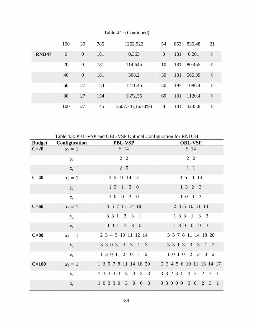
89
Table 4.2: (Continued)
Table 4.3: PBL-VSP and OBL-VSP Optimal Configuration for RND 34
Budget Configuration PBL-VSP OBL-VSP
C=20 𝑥𝑖 = 1 5 14 5 14
𝑦𝑖 2 2 2 2
𝑧𝑖 2 0 1 1
C=40 𝑥𝑖 = 1 3 5 11 14 17 3 5 11 14
𝑦𝑖 1 3 1 3 0 1 3 2 3
𝑧𝑖 1 0 0 3 0 1 0 0 3
C=60 𝑥𝑖 = 1 3 5 7 11 14 18 2 3 5 10 11 14
𝑦𝑖 3 3 1 3 3 1 1 3 3 1 3 3
𝑧𝑖 0 0 1 3 3 0 1 3 0 0 0 3
C=80 𝑥𝑖 = 1 2 3 4 5 10 11 12 14 3 5 7 8 11 14 18 20
𝑦𝑖 3 3 0 3 3 3 1 3 3 3 1 3 3 3 1 2
𝑧𝑖 1 3 0 1 2 0 1 2 1 0 1 0 2 3 0 2
C=100 𝑥𝑖 = 1 1 3 5 7 8 11 14 18 20 2 3 4 5 6 10 11 13 14 17
𝑦𝑖 1 3 3 3 3 3 3 3 3 3 3 2 3 1 3 3 2 3 1
𝑧𝑖 1 0 3 3 0 3 0 0 3 0 3 0 0 0 3 0 2 3 1
100 30 785 1262.922 54 853 830.48
5
21
RND47 0 0 181 0.363 0 181 0.201 0
20 0 181 114.645 10 181 80.455 0
40 0 181 508.2 30 181 565.39
1
0
60 27 154 1211.45 50 197 1086.4
52
0
80 27 154 1372.35 60 181 1120.4
75
0
100 27 145 3607.74 (16.74%) 8 181 3245.8
5
0

90
CHAPTER 5: CONCLUSION
The studies presented in this dissertation have advanced the knowledge and techniques in
transportation system design and operations including vehicle scheduling, emergency medical
service network design and vehicle sharing program network design. Three critical transportation
problems are studied and discussed.
In chapter 2, we studied the scheduling problem for a bus fleet with alternative fuel
vehicles. In collaboration with a public transportation company, we successfully addressed a
practical problem in real life. We specifically study the cost characteristics of different types of
vehicles and consider the traffic congestion effects on fuel economy in the model. It is
demonstrated that the schedule generated by the model could significantly reduce total fleet size
required to finish timetables and balance the utilization of conventional diesel buses and
alternative fuel vehicles. Results show that the model provides a useful tool for transit provider
optimally allocating resources in their business operations.
In chapter 3, we studied emergency medical service network design problem to determine
the robust ambulance locations. Our study illustrated that traditional stochastic and probabilistic
models fail to capture all possible uncertain scenarios when the problem size is large. To address
this issue, we proposed two-stage robust optimization models. This special modeling technique
incorporates a compact uncertainty set and enables the decision maker to fully take advantage of
the revealed information to make less conservative decisions. The proposed model is the first
model to consider the impact of relocation operations on the initial locations. Furthermore,
91
classical algorithms have limited capability of handling two-stage robust optimization model
with mixed integer recourse problem, an approximate column-and-constraint generation
algorithm was developed and implemented. We conducted numerical experiments on a practical-
scale instance with real world data. Results show our method has strong capability of producing
either optimal solution or solutions with very small optimality gaps.
In chapter 4, a novel research topic studies critical limitations that recently have been
found in traditional bi-level optimization problems. We demonstrated that the regular optimistic
bi-level programming model unable to identify the uncertainty introduced by the lower level
model from the non-cooperative and non-unique issues. This counterintuitive finding totally
overthrows our understanding of bi-level programming. We further developed a pessimistic
optimization model that can derive solutions which are robust in any uncertain situations. A bi-
level relaxation and relaxation-and-correction computational scheme are proposed for finding
solutions that are both feasible and optimal to the pessimistic optimization model. Our
experiments are conducted on three widely adopted prototypical transportation networks with
several instances. Solutions are compared with that from optimistic formulation. Results
demonstrated that the pessimistic optimization model has great potential in designing a robust
and reliable vehicle sharing program network.
92
REFERENCES
[1] OECD Publishing, "IEA. Key world energy statistics," 2009. [Online]. Available:
http://dx.doi.org/10.1787/9789264039537-en. [Accessed may 2012].
[2] L. Bodin and B. Golden, "Classification in vehicle routing and scheduling," Networks, vol.
11, no. 2, p. 97–108., 1981.
[3] J. Renaud, G. Laporte and F. F. Boctor, "A tabu search heuristic for the multi-depot vehicle
routing problem.," Computers & Operations Research,, vol. 23, no. 3, pp. 229-235, 1996.
[4] G. Desaulniers, J. Lavigne and F. Soumis., "Multi-depot vehicle scheduling problems with
time windows and waiting costs," European Journal of Operational Research, vol. 111, no.
3, pp. 479-494, 1998.
[5] B. Ombuki-Berman and F. T. Hanshar, "Using genetic algorithms for multi-depot vehicle
routing," in Bio-inspired algorithms for the vehicle routing problem, vol. 161, Berlin
Heidelberg, Springer, 2009, pp. 77-99.
[6] J.-Q. Li and K. L. Head, "Sustainability provisions in the bus-scheduling problem,"
Transportation Research Part D: Transport and Environment, vol. 14, no. 1, pp. 50-60,
2009.

93
[7] Q. Wang, "Chinas energy end use and efficiency in 2007," Energy Saving and Environment
Protection (02), pp. 14-17, 2009.
[8] X. Yan and R. J. Crookes, "Reduction potentials of energy demand and ghg emissions in
china's road transport sector," Energy Policy, vol. 37, no. 2, pp. 658-668, 2009.
[9] G. Wan, "Thinking on chinese energy-saving and new energy vehicle development mode
and the initiatives," Traffic and Transportation, vol. 2, no. 1-3, 2008.
[10] H. Wang and M. Ouyang, "Transition strategy of the transportation energy and powertrain
in china," Energy Policy, vol. 35, no. 4, pp. 2313-2319, 2007.
[11] S. c. o. China, "The guide of accelerating the implementation of alternative fuel vehicles,"
14 7 2014. [Online]. Available: http://www.gov.cn/zhengce/content/2014-
07/21/content_8936.htm. [Accessed August 2014].
[12] www.ce.cn, "The development of alternative fuel vehicles in public transit," 18 3 2014.
[Online]. Available: http://auto.ce.cn/auto/gundong/201403/18/t20140318_2500241.shtml.
[Accessed 4 5 2014].
[13] X. Ou, X. Zhang and S. Chang, "Alternative fuel buses currently in use in china: life-cycle
fossil energy use, ghg emissions and policy recommendations.," Energy Policy, vol. 38, no.
1, pp. 406-418, 2010.
[14] M. Barth and K. Boriboonsomsin, "Traffic congestion and greenhouse gases," ACCESS
Magazine, p. 1(35), 2009.
[15] G.-H. Tzeng, C.-W. Lin and S. Opricovic, "Multi-criteria analysis of alternative-fuel buses
for public transportation," Energy Policy, vol. 33, no. 11, pp. 1373-1383, 2005.

94
[16] A. A. Bertossi, P. Carraresi and G. Gallo, "On some matching problems arising in vehicle
scheduling models," Networks, vol. 17, no. 3, pp. 271-281, 1987.
[17] C. A. Hane, C. Barnhart, E. L. Johnson, R. E. Marsten, G. L. Nemhauser and G.
Sigismondi, "The fleet assignment problem: solving a large-scale integer program,"
Mathematical Programming, vol. 70, no. 1-3, pp. 211-232, 1995.
[18] N. Kliewer, T. Mellouli and L. Suhl, "A new solution model for multi-depot multi-vehicle-
type vehicle scheduling in (sub) urban public transport," in Proceedings of the 13th Mini-
EURO Conference and the 9th meeting of the EURO working group on transportation,
Politechnic of Bari, 2002.
[19] J. M.Grutter, "The operations of hybrid and electric buses," 2014. [Online]. Available:
https://www.yumpu.com/nl/document/view/37197938/hybrid-and-electric-buses-in-
chinese/25.
[20] I. D. Greenwood and C. R. Bennett, "The effects of traffic congestion on fuel
consumption," Road and Transport Research, vol. 5, no. 2, 1996.
[21] L. Brotcorne, G. Laporte and F. Semet, "Ambulance location and relocation models,"
European journal of operational research, vol. 147, no. 3, pp. 451-463, 2003.
[22] C. ReVelle, D. Bigman, D. Schilling, J. Cohon and R. Church, "Facility location: a review
of context-free and ems models," Health Services Research, vol. 12, no. 2, p. 129, 1977.
[23] D. Williams, "2004 jems 200-city survey," JEMS: a journal of emergency medical
services, vol. 30, no. 2, p. 42, 2005.
[24] M. Gendreau, G. Laporte and F. Semet, "Solving an ambulance location model by tabu
search," Location science, vol. 5, no. 2, pp. 75-88, 1997.

95
[25] T. WlSBORG, A. Guttormsen, M. Sorensen and H. Flaatten, "The potential of an
anaesthesiologist{manned ambulance service in a rural/urban district," Acta
anaesthesiologica scandinavica, vol. 38, no. 7, pp. 657-661, 1994.
[26] M. S. Daskin, "A maximum expected covering location model: formulation, properties and
heuristic solution," Transportation Science, vol. 17, no. 1, pp. 48-70, 1983.
[27] J. F. Repede and J. J. Bernardo., "Developing and validating a decision support system for
locating emergency medical vehicles in louisville, kentucky," European Journal of
Operational Research, vol. 75, no. 3, pp. 567-581, 1994.
[28] R. Batta, J. M. Dolan and N. N. Krishnamurthy, "The maximal expected covering location
problem: Revisited," Transportation Science, vol. 23, no. 4, pp. 277-287, 1989.
[29] V. Marianov and C. Revelle, "The queuing probabilistic location set covering problem and
some extensions," Socio-Economic Planning Sciences, vol. 28, no. 3, pp. 167-178, 1994.
[30] M. O. Ball and F. L. Lin, "A reliability model applied to emergency service vehicle
location," Operations Research, vol. 41, pp. 18-36, 1993.
[31] R. L. Larson and T. W. Hilde., "A revised time scale of magnetic reversals for the early
cretaceous and late jurassic," Journal of Geophysical Research, vol. 80, no. 17, pp. 2586-
2594, 1975.
[32] A. Ben-Tal, L. E. Ghaoui and A. Nemirovski, Robust optimization., 2009.
[33] H.-G. Beyer and B. Sendho, "Robust optimization- a comprehensive survey.," Computer
methods in applied mechanics and engineering, vol. 196, no. 33, pp. 3190-3218, 2007.
[34] D. Bertsimas, D. B. Brown and C. Caramanis., "Theory and applications of robust
optimization," SIAM review, vol. 53, no. 3, pp. 464-501, 2011.
96
[35] L. V. Snyder, "Facility location under uncertainty: a review," IIE Transactions, vol. 38, no.
7, pp. 547-564, 2006.
[36] C. ReVelle and K. Hogan, "The maximum availability location problem," Transportation
Science, vol. 23, no. 3, pp. 192-200, 1989.
[37] P. B. a. M. E. Bruni, "A probabilistic model applied to emergency service vehicle
location," European Journal of Operational Research, vol. 196, no. 1, pp. 323-331, 2009.
[38] P. Beraldi, M. E. Bruni and D. Conforti, "Designing robust emergency medical service via
stochastic programming," European Journal of Operational Research, vol. 158, no. 1, pp.
183-193, 2004.
[39] Y. An, B. Zeng, Y. Zhang and L. Zhao, "Reliable p-median facility location problem: two-
stage robust models and algorithms," Transportation Research Part B: Methodological,
vol. 64, pp. 54-72, 2014.
[40] C. Toregas, R. Swain, C. ReVelle and L. Bergman, "The location of emergency service
facilities," Operations Research, vol. 19, no. 6, pp. 1363-1373, 1971.
[41] R. Church and C. ReVelle, "The maximal covering location problem," Papers in regional
science, vol. 32, no. 1, pp. 101-118, 1974.
[42] D. Schilling, D. J. Elzinga, J. Cohon, R. Church and C. ReVelle, "The team/fleet models
for simultaneous facility and equipment siting.," Transportation Science, vol. 13, no. 2, pp.
163-175, 1979.
[43] M. S. Daskin and E. H. Stern, "A hierarchical objective set covering model for emergency
medical service vehicle deployment," Transportation Science, vol. 15, no. 2, pp. 137-152,
1981.
97
[44] K. Hogan and C. ReVelle, "Concepts and applications of backup coverage," Management
science, vol. 32, no. 11, pp. 1434-1444, 1986.
[45] K. F. Doerner, W. J. Gutjahr, R. F. Hartl, M. Karall and M. Reimann, "Heuristic solution of
an extended double-coverage ambulance location problem for Austria," Central European
Journal of Operations Research, vol. 13, pp. 325-340, 2005.
[46] G. Laporte, F. V. Louveaux, F. Semet and A. Thirion, "Application of the double standard
model for ambulance location," Innovations in distribution logistics, pp. 235-249, 2009.
[47] V. Schmid and K. F. Doerner, "Ambulance location and relocation problems with time-
dependent travel times," European journal of operational research, vol. 207, pp. 1293-
1303, 2010.
[48] K. Kepaptsoglou, M. G. Karlaftis and G. Mintsis, "Model for planning emergency response
services in road safety," Journal of Urban Planning and Development, vol. 138, pp. 18-25,
2011.
[49] Y. Liu, A. M. Roshandeh, Z. Li, K. Kepaptsoglou, H. Patel and X. Lu, "Heuristic approach
for optimizing emergency medical services in road safety within large urban networks,"
Journal of Transportation Engineering, vol. 140, no. 9, p. 04014043, 2014.
[50] R. C. Larson, "A hypercube queuing model for facility location and redistricting in urban
emergency services," Computers \& Operations Research, vol. 1, no. 1, pp. 67-95, 1974.
[51] C. Saydam and H. Aytu{\u{g}}, "Accurate estimation of expected coverage: revisited,"
Socio-Economic Planning Sciences, vol. 37, no. 1, pp. 69-80, 2003.

98
[52] R. D. Galvão, F. Y. Chiyoshi and R. Morabito, "Towards unified formulations and
extensions of two classical probabilistic location models," Computers & Operations
Research, vol. 32, no. 1, pp. 15-33, 2005.
[53] A. P. Iannoni, R. Morabito and C. Saydam, "A hypercube queueing model embedded into a
genetic algorithm for ambulance deployment on highways," Annals of Operations
Research, vol. 157, no. 1, pp. 207-224, 2008.
[54] A. P. Iannoni, R. Morabito and C. Saydam, "An optimization approach for ambulance
location and the districting of the response segments on highways," European Journal of
Operational Research, vol. 195, no. 2, pp. 528-542, 2009.
[55] A. Shariat-Mohaymany, M. Babaei, S. Moadi and S. M. Amiripour, "Linear upper-bound
unavailability set covering models for locating ambulances: Application to Tehran rural
roads," European Journal of Operational Research, vol. 221, no. 1, pp. 263-272, 2012.
[56] H. Davoudpour, E. Mortaz and S. Hosseinijou, "A new probabilistic coverage model for
ambulances deployment with hypercube queuing approach," The International Journal of
Advanced Manufacturing Technology, vol. 70, no. 5-8, pp. 1157-1168, 2014.
[57] P. Beraldi and M. E. Bruni, "A probabilistic model applied to emergency service vehicle
location," European Journal of Operational Research, vol. 196, no. 1, pp. 323-331, 2009.
[58] K. Schneeberger, K. F. Doerner, A. Kurz and M. Schilde, "Ambulance location and
relocation models in a crisis," Central European Journal of Operations Research, vol. 24,
no. 1, pp. 1-27, 2016.
99
[59] B. Zeng and L. Zhao, "Solving two-stage robust optimization problems using a constraint-
and-column generation method," University of South Florida, Technical Report, available
in optimization-online, 2011.
[60] United States Census Bureau, "United States Census Bureau," United States Census
Bureau, 2015. [Online]. Available: http://www.census.gov/. [Accessed 2 Sep 2015].
[61] S. Shaheen, S. Guzman and H. Zhang, "Bikesharing in Europe, the Americas, and Asia
Past, Present, and Future," Transportation Research Record: Journal of the Transportation
Research Board, vol. 2143, no. 20, pp. 159-167, 2014.
[62] S. A. Shaheen and A. P. Cohen, "Growth in Worldwide Carsharing," Transportation
Research Record: Journal of the Transportation Research Board (2007):, pp. 81-89, 2007.
[63] S. A. Shaheen, M. Meyn and K. Wipyewski, "U.S. Shared-use vehicle survey findings on
carsharing and station car growth," Transportation research record, vol. 03, no. 4469, pp.
90-98, 2003.
[64] R. Nair and E. Miller-Hooks, "Equilibrium network design of shared-vehicle systems,"
European journal of operational research, vol. 235, pp. 47-61, 2014.
[65] A. Millard-Ball, Car-Sharing: Where and how it succeeds, vol. 108, Transportation
Research Board, 2005.
[66] D. Friedman, "Public vehicle rental system: Determination of feasibility.," in selected
proceedings of a conference on methods and concepts of forecasting travel demands, 1972.
[67] R. Katzev, "Car Sharing: A New Approach to Urban Transportation Problems,"
Transportation research record, vol. 3, no. 1, pp. 65-86, 2003.

100
[68] S. d. Luca and R. D. Pace, "Modelling users’ behaviour in inter-urban carsharing program:
A stated preference approach," Transportation Research Part A: Policy and Practice, vol.
71, pp. 59-76, 2015.
[69] M. Namazu and H. Dowlatabadi, "Characterizing the GHG emission impacts of carsharing:
a case of Vancouver," Environmental Research Letters, vol. 10, no. 12, 2015.
[70] P. Baptista, S. Melo and C. Rolim, "Car Sharing Systems as a Sustainable Transport
Policy: A Case Study from Lisbon, Portugal," in Transport and Sustainability, Emerald
Group Publishing Limited, 2015, pp. 205-227.
[71] R. Nair and E. Miller-Hooks, "Fleet Management for Vehicle Sharing Operations,"
Transportation science, vol. 45, no. 4, pp. 524-540, 2011 .
[72] J. Shu, M. Chou, Q. Liu, C.-P. Teo and I.-L. Wang, "Bicycle-sharing system: deployment,
utilization and the value of re-distribution," National University of Singapore-NUS
Business School, Singapore, 2010.
[73] A. Kek, R. Cheu and M. Chor, "Relocation Simulation Model for Multiple-Station Shared-
Use Vehicle Systems," Transportation Research Record: Journal of the Transportation
Research Board, No.1986, pp. 81-88, 2006.
[74] M. Rainer-Harbach, P. Papazek, B. Hu and G. R. Raidl, "Balancing Bicycle Sharing
Systems: A Variable Neighborhood Search Approach," in Evolutionary Computation in
Combinatorial Optimization: 13th European Conference, EvoCOP 2013, Vienna, Austria,
April 3-5, 2013. Proceedings, Berlin, Heidelberg, Springer Berlin Heidelberg, 2013, pp.
121-132.
101
[75] I. A. Forma, T. Raviv and M. Tzur, "A 3-step math heuristic for the static repositioning
problem in bike-sharing systems," Transportation Research Part B: Methodological, vol.
71, pp. 230-247, 2015.
[76] P. Angeloudis, J. Hu and M. G. Bell, "A strategic repositioning algorithm for bicycle-
sharing schemes," Transportmetrica A: Transport Science, vol. 10, no. 8, pp. 759-774,
2014.
[77] J. Shu, M. C. Chou, Q. Liu, C.-P. Teo and I.-L. Wang, "Models for effective deployment
and redistribution of bicycles within public bicycle-sharing systems," Operations Research,
vol. 61, no. 6, pp. 1346-1359, 2013.
[78] A. Awasthi, D. Breuil, S. S. Chauhan, M. Parent and T. Reveillere, "A Multicriteria
Decision Making Approach for Carsharing Stations Selection," Journal of Decision
Systems, vol. 16, no. 1, pp. 57-78, 2007.
[79] d. A. Correia, G. Homem and A. P. Antunes, "Optimization approach to depot location and
trip selection in one-way carsharing systems," Transportation Research Part E: Logistics
and Transportation Review, vol. 48, no. 1, pp. 233-247, 2012.
[80] L. dell'Olio, A. Ibeas and J. L. Moura, "implementing bike-sharing systems," Proceedings
of the Institution of Civil Engineers - Municipal Engineer, vol. 164, no. 2, pp. 89-101,
2011.
[81] J. Lin and T. Yang, "Strategic design of public bicycle sharing systems with service level
constraints," Transportation Research Part E, vol. 47, no. 2, pp. 284-294, 2011.
102
[82] L. M. Martinez, L. Caetano, T. Eir o and F. Cruz, "An Optimisation Algorithm to Establish
the Location of Stations of a Mixed Fleet Biking System: An Application to the City of
Lisbon.," in Proceedings of EWGT2012 - 15th Meeting of the EURO Working Group on
Transportation, , Paris, 2012.
[83] B. Zeng, "Easier than we thought-a practical scheme to compute pessimistic bilevel
optimization problem," Available at SSRN 2658342, 2015.
[84] M. F. Heinz Spiess, "Optimal strategies: A new assignment model for transit networks,"
Transportation research part B, vol. 23, no. 2, pp. 83-102, 1989.
[85] C. Audet, P. Hansen, B. Jaumard and G. Savard, "Links between linear bilevel and mixed
0-1 programming problems," Journal of Optimization Theory and Applications, vol. 93, no.
2, pp. 273-300, 1997.
[86] J. Bard, Practical bilevel optimization: algorithms and applications, Springer, 1998.
[87] S. Dempe, Foundations of bilevel programming, Springer, 2002.
[88] M. Moeini, Z. Jemai and E. Sahin, "Location and relocation problems in the context of the
emergency medical service systems: a case study," Central European Journal of
Operations Research, vol. 23, no. 3, pp. 641-658, 2015.
[89] Z. Zhang and H. Jiang, "A robust counterpart approach to the bi-objective emergency
medical service design problem," Applied Mathematical Modelling, vol. 38, no. 3, pp.
1033-1040, 2013.