Decision Guidance for Sustainable Manufacturing

DECISION GUIDANCE FOR SUSTAINABLE MANUFACTURING

by

Guodong Shao

A Dissertation

Submitted to the

Graduate Faculty

of

George Mason University

in Partial Fulfillment of

The Requirements for the Degree

of

Doctor of Philosophy

Information Technology

Committee:

Dr. Alexander Brodsky, Dissertation Co-

Director

Dr. Paul Ammann, Dissertation Co-Director

Dr. Daniel Menascé, Committee Member

Dr. David Schum, Committee Member

Dr. Stephen Nash, Senior Associate Dean

Dr. Kenneth S. Ball, Dean, Volgenau School

of Engineering

Date: Spring Semester 2013


Fairfax, VA

http://volgenau.gmu.edu/about_ite/associate_dean_research_graduate_studies.php

Decision Guidance for Sustainable Manufacturing

A dissertation submitted in partial fulfillment of the requirements for the degree of

Doctor of Philosophy at George Mason University

by

Guodong Shao

Master of Engineering

University of Maryland, 1999

Dissertation Directors: Alexander Brodsky and Paul Ammann, Associate Professors

Department of Information Technology

Spring Semester 2013


Fairfax, VA

ii

This work is licensed under a creative commons

attribution-noderivs 3.0 unported license.

http://creativecommons.org/licenses/by-nd/3.0/

http://creativecommons.org/licenses/by-nd/3.0/

iii

DEDICATION

This is dedicated to my loving wife Julia, my two wonderful children John and Joy.

iv

ACKNOWLEDGEMENTS

I would like to thank all those people who have made this dissertation possible. I would

like to begin by thanking my dissertation directors Dr. Brodsky and Dr. Ammann for

their outstanding guidance and patience along the way. They have been always there to

listen and give advice. I have worked very closely with Dr. Brodsky and learned a lot

from him. I am also indebted to my committee members Dr. Menascé and Dr. Schum for

their time and invaluable help.

I am grateful to my friend Nathan Egge for his support for the DGQL programming and

Chun-Kit Ngan for OPL support. I also would like to acknowledge many of my

colleagues from National Institute of Standards and Technology (NIST) for discussions

and managers for their encouragement and supports. Specifically, many thanks to Tina

Yung-Tsun Lee for her help in dissertation proofreading.

Most importantly, none of this would have been possible without the love, support, and

patience of my family for all these years. I would like to express my sincere gratitude to

my family.

v

TABLE OF CONTENTS

Page

List of Tables .................................................................................................................... vii

List of Figures .................................................................................................................. viii

List of Equations ................................................................................................................. x

List of Abbreviations ......................................................................................................... xi

Abstract ............................................................................................................................ xiii

1. Introduction ................................................................................................................. 1

1.1 Sustainable Manufacturing: Motivation and Background ........................................ 1

1.2 Research Gap............................................................................................................. 3

1.3 Problem Statement and Dissertation Research Objectives ..................................... 10

1.4 Thesis Statement and Summary of Contributions ................................................... 11

1.5 Resulting Publications ............................................................................................. 12

1.6 Thesis Structure ....................................................................................................... 14

2. Related work .............................................................................................................. 16

2.1 Sustainable Manufacturing Efforts.......................................................................... 16

2.2 Decision Support Methodologies ............................................................................ 20

2.3 Process Modeling Methodologies ........................................................................... 27

3. Sustainable Process Description And Analytics (SPDA) Formalism .......................... 32

3.1 The Concept of SPDA Formalism within a SM Improvement Methodology ........ 32

3.2 SPDA High-Level Design Requirements and Layers of Abstraction ..................... 35

3.3 SPDA Formalism by Example ................................................................................ 39

3.4 SPDA Syntax and Semantics .................................................................................. 63

3.5 SPDA Query Computation ...................................................................................... 79

3.6 SPDA Features Summary........................................................................................ 85

4. Methodology ................................................................................................................. 87

4.1 Formulation of High Level Problem ....................................................................... 91

4.2 Acquisition of Domain Knowledge......................................................................... 91

vi

4.3 Design of Conceptual Model................................................................................... 92

4.4 Collection of Data ................................................................................................... 93

4.5 Building of SPDA models ....................................................................................... 96

4.6 What-if analysis and Optimization Query using SPDA ........................................ 105

4.7 Actionable Recommendation ................................................................................ 107

5. Case studies ................................................................................................................. 109

5.1 Classification of potential SM case studies using SPDA ...................................... 109

5.2 Case Study 1 - Investment/planning for Energy Efficient Manufacturing............ 114

5.3 Case Study 2 - Operational control for sustainable machining ............................. 140

6. Conclusion .................................................................................................................. 161

Appendix A – Proof of Claim 1 (Correctness of SPDA query computation algorithm) 164

Appendix B – OPL code for case study of Investment/planning for Energy Efficient

Manufacturing ................................................................................................................. 167

Appendix C – Publications ............................................................................................. 174

References ....................................................................................................................... 182

vii

LIST OF TABLES

Table Page

Table 1 A comparison table for modeling languages with desirable features .................... 9 Table 2 A comparison of SPDA with other languages contrasting desirable features ..... 85

Table 3 An example tariff table ...................................................................................... 116

Table 4 Descriptions of constant data ............................................................................. 119

Table 5 Evaluation parameters of ROI ........................................................................... 139 Table 6 Evaluation parameters of GHG emissions ......................................................... 139 Table 7 Speed – time – emission table............................................................................ 152

viii

LIST OF FIGURES

Figure Page

Figure 1 The triple bottom line of sustainability – balancing social, environmental, and

economic factors (source: (Adams, 2006)) ......................................................................... 2

Figure 2 Current analysis modeling approach .................................................................... 7

Figure 3 Outline and structure of the thesis ...................................................................... 15

Figure 4 A SM improvement methodology with the support of SPDA formalism .......... 34 Figure 5 Current modeling approaches and the unified SPDA modeling approach ......... 37 Figure 6 Sustainable process description and analytics formalism layers of abstraction . 39 Figure 7 SPDA Process description model components................................................... 41

Figure 8 An example: a two-product-manufacturing process ........................................... 42 Figure 9 A what-if analysis query for the two-product-manufacturing process ............... 44

Figure 10 Optimization query for the two-product-manufacturing process ..................... 45 Figure 11 Context model for the two-product-manufacturing example ........................... 46 Figure 12 Flow model for the two-product-manufacturing example ................................ 47

Figure 13 Flow aggregator model for the two-product-manufacturing example ............. 48 Figure 14 Atomic process model for the two-product-manufacturing example ............... 49

Figure 15 Atomic process model for Machine A.............................................................. 51

Figure 16 Atomic process model for Machine B .............................................................. 52

Figure 17 Atomic process model for Machine C .............................................................. 53 Figure 18 Atomic process model for Assembly A............................................................ 54

Figure 19 Atomic process model for Assembly B ............................................................ 54 Figure 20 Generic composite process model .................................................................... 56

Figure 21 Metric aggregator model .................................................................................. 57 Figure 22 Composite process model for the two-product-manufacturing process ........... 59 Figure 23 A context data sequence for the two-product-manufacturing process ............. 60 Figure 24 Product demand data model for product 1 and product 2 ................................ 60

Figure 25 What-if query for the two-product-manufacturing example ............................ 61 Figure 26 Optimal solution screen of two-product-manufacturing example .................... 63 Figure 27 SPDA formalism class diagram – generic analytics language ......................... 65

Figure 28 A hierarchical diagram for the Process Description and Sustainability Metrics

........................................................................................................................................... 66 Figure 29 SPDA component library: example of generic models .................................... 68 Figure 30 SPDA component library: examples of specific models .................................. 68 Figure 31 A commutative diagram for analytical query computation .............................. 80

Figure 32 Algorithm 1: SPDA query computation ........................................................... 82 Figure 33 Algorithm 2: optimization sequence algorithm (OptSeqAlg) .......................... 84

ix

Figure 34 Concept of the decision guidance management system for sustainable

manufacturing using the SPDA formalism ....................................................................... 87 Figure 35 Use case for implementation of decision guidance management system using

the SPDA formalism ......................................................................................................... 89

Figure 36 A model based decision guidance methodology for sustainable manufacturing

........................................................................................................................................... 90 Figure 37 Context model flowchart .................................................................................. 98 Figure 38 Flow model flowchart....................................................................................... 99 Figure 39 Flow aggregator model flowchart .................................................................. 100

Figure 40 Generic atomic model flowchart .................................................................... 101 Figure 41 Atomic process instance model flowchart ...................................................... 102 Figure 42 Composite process model flowchart .............................................................. 104

Figure 43 SPDA query model flowchart ........................................................................ 105 Figure 44 Steps for solving an SPDA query in a decision guidance management system

......................................................................................................................................... 106

Figure 45 Aggregation of sustainability factors for hierarchical production levels ...... 110 Figure 46 Prospective heating, cooling, and electric facilities diagram ......................... 117

Figure 47 Context model of facility heating/cooling and power case study................... 125 Figure 48 Flow model of facility heating/cooling and power case study ...................... 125 Figure 49 Flow aggregator model of facility heating/cooling and power case study .... 126

Figure 50 Electricity supply process model of facility heating/cooling and power case

study ................................................................................................................................ 128

Figure 51 Gas process model of facility heating/cooling and power case study ........... 130 Figure 52 Current heat and cooling process model of facility heating/cooling and power

case study ........................................................................................................................ 132

Figure 53 Co-gen process model of facility heating/cooling and power case study ..... 134

Figure 54 Composite process model of facility heating/cooling and power case study 137 Figure 55 Query of facility heating/cooling and power case study ............................... 138 Figure 56 Sustainable machining SPDA modeling diagram .......................................... 142

Figure 57 Machining process input and output flows diagram....................................... 142 Figure 58 An example of a real machining center and its virtual model (Shao & Lee,

2007) ............................................................................................................................... 143 Figure 59 Dependency graph model for cutting speed vs. CO2 emission ...................... 149

Figure 60 Experimental emission data from both process and cutting tool .................... 151 Figure 61 Experimental data for speed, cutting time, and tool life ................................. 152 Figure 62 Flow model for the machining case............................................................... 153 Figure 63 An atomic sustainable milling machining process model .............................. 155

Figure 64 Composite process model for milling process................................................ 156 Figure 65 Data model of the sustainable machining case .............................................. 157 Figure 66 An optimization query of emission for the sustainable machining case ...... 158

Figure 67 OPL model screen capture for the sustainable machining case ..................... 159 Figure 68 Optimization results of machining time using IBM ILOG CPLEX ............... 159

x

LIST OF EQUATIONS

Equation Page

Equation 1 Savings ......................................................................................................... 122 Equation 2 Payback period ............................................................................................. 122

Equation 3 Return on investment .................................................................................... 122

Equation 4 kWh charge for 0 ≤ kWh ≤ 24000................................................................ 122

Equation 5 kWh charge for 24000 ≤ kWh is ≤ 210000 .................................................. 122

Equation 6 kWh charge for 24000 ≤ kWh is ≤ 210000 .................................................. 122

Equation 7 total gas cost ................................................................................................. 123

Equation 8 GHG emissions ............................................................................................. 123 Equation 9 Cogen gas kWh conversion .......................................................................... 123

Equation 10 Total environmental impact ........................................................................ 144 Equation 11 Total electricity consumption of machine tool ........................................... 144 Equation 12 The environmental impact of coolant ......................................................... 145

Equation 13 The environmental impact of coolant with water-insoluble cutting fluid .. 146 Equation 14 The environmental impact of lubricant oil ................................................. 146

Equation 15 The environmental impact of cutting tool .................................................. 147 Equation 16 The environmental impact of metal chips .................................................. 147

Equation 17 CO2 emissions due to the cutting process................................................... 150 Equation 18 CO2 emissions resulting from the cutting tool ........................................... 150 Equation 19 Total emission ............................................................................................ 150

Equation 20 Taylor tool life equation ............................................................................. 150 Equation 21 Generic version of Taylor tool life equation .............................................. 150

Equation 22 Tool cutting speed ...................................................................................... 160 Equation 23 Tool feed rate .............................................................................................. 160

xi

LIST OF ABBREVIATIONS

Automated Guided Vehicle........................................................................................... AGV

A Modeling Language for Mathematical Programming ........................................... AMPL

Automated Storage/Retrieval Systems ....................................................................... ASRS

Business Process Execution Language ....................................................................... BPEL

Business Process Model and Notation ....................................................................... BPMN

Centralized Heating and Cooling Plant ...................................................................... CHCP

Combined Heating and Power ...................................................................................... CHP

Computer Aided Design ............................................................................................... CAD

Computer Aided Manufacturing .................................................................................. CAM

Constraint Optimization Regression in Java ........................................................ CoReJava

Constraint Programming ................................................................................................... CP

Core Manufacturing Simulation Data ....................................................................... CMSD

Discrete Event Simulation ............................................................................................. DES

Decision Guidance Management System .................................................................. DGMS

Decision Guidance Query Language .......................................................................... DGQL Department of Commerce .............................................................................................. DOC European Commission Life Cycle Database .............................................................. ELCD

Energy Information Administration ................................................................................ EIA

Energy Management System ........................................................................................ EMS

Enterprise Resource Planning ........................................................................................ ERP

Explicit Process Structure and Data ............................................................................. EPSD

General Algebraic Modeling System ......................................................................... GAMS

Greenhouse Gas ........................................................................................................... GHG

Graphical User Interface ................................................................................................ GUI

Heating, Ventilation, and Air Conditioning ............................................................... HVAC

Hypertext Markup Language ..................................................................................... HTML

Implicit Process Structure and Data ............................................................................. IPSD

Internet Protocol................................................................................................................. IP

Java Database Connectivity Application Programming Interface ........................ JDBCAPI

Java Server Pages .............................................................................................................JSP

Kilowatts .......................................................................................................................... kW

Kilowatts-hours .............................................................................................................. kWh

Key Performance Indicator ............................................................................................. KPI

Life Cycle Assessment ...................................................................................................LCA

Life Cycle Inventory ....................................................................................................... LCI

Linear Programming ......................................................................................................... LP

http://en.wikipedia.org/wiki/Business_Process_Execution_Language

http://en.wikipedia.org/wiki/Internet_Protocol

http://en.wikipedia.org/wiki/Application_programming_interface

xii

Master Production Schedule ..........................................................................................MPS

Mathematical Programming............................................................................................. MP

Manufacturing Execution Systems ............................................................................... MES

Metric Tons of Carbon Dioxide Equivalent .............................................................. MTCDE Mixed Integer Linear Programming ............................................................................... MILP Numerical Control ........................................................................................................... NC

National Institute of Standards and Technology ........................................................... NIST

Organization for Economic Co-operation and Development ..................................... OECD

Object Linking and Embedding for Process Control ..................................................... OPC

Object Management Group ......................................................................................... OMG

Operations Research ........................................................................................................ OR

Probability Density Function ......................................................................................... PDF

Product Data Management ............................................................................................ PDM

Programmable Logic Controller .................................................................................... PLC

Regression Analysis ......................................................................................................... RA

Relational Database Management System ...............................................................RDBMS

Return on Investment ..................................................................................................... ROI

Simulation Interoperability Standards Organization ................................................... SISO

Structured Query Language ........................................................................................... SQL

Sustainable Manufacturing ............................................................................................. SM

Sustainable Process Description and Analytics ......................................................... SPDA

Systems Modeling Language ..................................................................................... SysML

Tariff Rate Schedule ...................................................................................................... TRS

Unified Modeling Language ......................................................................................... UML

Unit Process Life Cycle Inventory ............................................................................. UPLCI

eXtensible Markup Language ....................................................................................... XML

xiii

ABSTRACT

DECISION GUIDANCE FOR SUSTAINABLE MANUFACTURING

Guodong Shao, Ph.D.

George Mason University, 2013

Dissertation Co-Directors: Dr. Alexander Brodsky and Dr. Paul Ammann

Sustainable manufacturing has significant impacts on a company’s business performance

and competitiveness in today’s world. A growing number of manufacturing industries are

initiating efforts to address sustainability issues; however, to achieve a higher level of

sustainability, manufacturers need methodologies for formally describing, analyzing,

evaluating, and optimizing sustainability performance metrics for manufacturing

processes and systems. Currently, such methodologies are missing.

This dissertation developed the Sustainable Process Description and Analytics

(SPDA) formalism and a systematic decision guidance methodology to fill the research

gaps. The methodology provides step-by-step guidance for sustainability performance

analysis and decision optimization using the SPDA formalism. The SPDA formalism

supports unified syntax and semantics for querying, what-if analysis, and decision

optimization; enables modular, extensible, and reusable modeling; enables built-in

process and sustainability metrics modeling that allows users using data from production,

xiv

energy management, life cycle assessment reference database for modeling and analysis;

and is easy to use by manufacturing and business users. Reduction procedures are

developed to enable the translations of the SPDA query into specialized models such as

optimization or simulation model for decision guidance. Two sustainable manufacturing

case studies have been performed to demonstrate the use of formalism and the

methodology.

1

1. INTRODUCTION

1.1 Sustainable Manufacturing: Motivation and Background This dissertation research develops the Sustainable Process Description and Analytics

(SPDA) formalism and a decision guidance methodology to help manufacturers achieve

their Sustainable Manufacturing (SM) goal in a systematic and quantitative manner.

To be successful in today's complex, rapidly changing, and highly competitive

world, manufacturers must use sustainable practices throughout their manufacturing

operations. Sustainability has been defined as “development that meets the needs of the

present without compromising the ability of future generations to meet their own needs

(World Commission on Environment and Development, 1987).” Harvard Business

Review declares “There is no long-term alternative to sustainable development

(Nidumolu, Prahalad, & Rangaswami, 2009).” An extensive study by MIT Sloan

Management Review found that “there is a strong consensus that sustainability is having

– and will continue to have – a material impact on how companies think and act (MIT

Sloan Management Review, 2010).” The United States Department of Commerce (DOC)

identified sustainable manufacturing as one of its high-priority performance goals,

defining SM as the “creation of manufactured products that use processes that minimize

negative environmental impacts, conserve energy and natural resources, are safe for

employees, communities, and consumers and are economically sound (DOC 2010).” This

means that the needs of the manufacturer should be balanced against the environmental,

http://www.1000ventures.com/business_guide/crosscuttings/new_economy_transition.html

http://www.1000ventures.com/business_guide/crosscuttings/new_economy_transition.html

2

economic, and social factors as shown in Figure 1. This dissertation focuses mainly on

supporting the environmental and economic aspects of SM.

Figure 1 The triple bottom line of sustainability – balancing social, environmental, and economic factors (source: (Adams, 2006))

Manufacturers’ wise decisions to support SM could not only lead to significant savings

for the company but also provide positive impact to the society and environment.

Increasingly, companies are employing practices that make their operations and

manufacturing processes more sustainable (Fujitsu 2011, GM 2010, Rockwell

Automation 2010). “Sustainability-related issues, such as energy consumption, emissions,

and other environmental impact, are becoming an increasingly integrated part of

operational and long-term planning decisions in manufacturing (Kuhl & Zhou, 2009).”

Among many of the sustainability-related issues, energy management is an

important sustainability factor. According to the National Association of Manufacturers

(NAM, 2010), the manufacturing sector currently accounts for about one third (33 %) of

http://secretaryofinnovation.com/2010/05/26/the-triple-bottom-line-of-sustainability/

3

all energy consumed in the United States, that is why many companies have paid

attention to energy efficiency. Lockheed Martin’s Go Green program indicated that a new

Energy Management System (EMS) in Camden reduced carbon emissions by 2,332

metric tons per year (NIST Workshop, 2010). SAIC has used its EMSs to realize

significant facility efficiencies for some auto manufacturers in the U.S. and monitor and

control nearly 20 million square feet of facility with millions of dollars in savings (SAIC,

2011).

Even though a growing number of manufacturing industries are initiating efforts

to address sustainability issues, most of them are targeting lower hanging fruits. A

systematic and quantitative approach is required to reach a higher level of sustainability.

Formalism and tools are needed to support a decision guidance methodology that

systematically guides problem identification, knowledge and data collection, formal

problem representation, what-if analysis and decision optimization, and recommendation

for improvement. To achieve these objectives, there are two main research gaps need to

be filled.

1.2 Research Gap Increasing the availability, use, and effectiveness of modeling, simulation, and

optimization technologies has been identified as a key enabler for improving SM in the

future (SMLC , 2011); however, using such technologies, especially for small and

medium-sized enterprises, presents some major challenges. These challenges, mainly due

to the complexity of modeling and optimization, have led to the underutilization of this

valuable technique, and in turn, affected the quality and effectiveness of decision-making.

4

Generally, research gaps and challenges include (1) the lack of systematic,

consistent, and quantitative methodology that enables effective sustainability

performance analysis and optimization and (2) the lack of unified process analytics

formalism to describe and represent sustainable process knowledge required for both

what-if analysis and decision optimization. A more detailed discussion is as follows.

Research gap 1: The lack of systematic, consistent, and quantitative methodology

that enables effective sustainability performance analysis and optimization.

Currently, most of the manufacturers’ projects are conducted on an ad hoc and

piecemeal basis for individual situations. The methods are customized, not integrated, not

reusable, and not extensible. The effect of many complex interactions is often not being

taken into account (Smith & Ball, 2012).

Different aspects of frameworks and methodologies that analyze and optimize

sustainability performance of manufacturing processes have been researched ( (Paju, et

al., 2010; Pineda-Henson & Culaba, 2002); however, a generic decision guidance

methodology that supports step-by-step sustainability performance analysis and decision

optimization is still missing.

Research gap 2: The lack of unified process analytics formalism to describe and

represent sustainable process knowledge required for what-if analysis and decision

optimization.

5

One of the challenges to use optimization techniques is that complex analysis

requires the development of formal simulation and/or optimization models, which

requires significant modeling expertise and substantial development effort due to the

complexity of both the problem and the tool. For example, modeling of a manufacturing

process using Mathematical Programming (MP) tools such as A Modeling Language for

Mathematical Programming (AMPL), an algebraic modeling language for linear and

nonlinear optimization problems in discrete or continuous variables (AMPL, 2011), or

Constraint Programming (CP) typically requires extensive Operation Research (OR) and

mathematical training. Normally, people from the factory floor do not have such

knowledge and training. There is a great need for making the modeling process easier and

reusing modeling efforts.

The lack of unified process analytics formalism to describe, represent, analyze,

and optimize sustainable processes makes it a particular challenge for users to model,

exchange, and reuse sustainability knowledge. Currently, different analysis tools such as

simulation, optimization, and database query languages require different data

representation and mathematical abstractions. Thus, even for the same manufacturing

process, the knowledge needs to be represented differently multiple times, rather than just

once. Figure 2 depicts such a modeling approach. Today, there is no existing analytical

formalism that allows users to model underlying reality once and reuse it for different

tasks including querying, what-if analysis, and decision optimization.

To understand the research gaps, a variety of modeling languages and formalisms,

listed in Table 1, are analyzed from the perspective of the following desirable features

6

and capabilities: (1) data manipulation and querying; (2) what-if analysis; (3)

optimization; (4) unified modeling capability; (5) built-in support for process

computation modeling and sustainable manufacturing process modeling; (6) modularity,

extensibility, and reusability; and (7) ease of use. These modeling languages/formalisms

include:

Process description languages such as Process Specification Language (PSL)

(Schlenoff, Gruninger, Creek, Ciocoiu, & Lee, 1999), Business Process Model and

Notation (BPMN) (OMG, 2010), and Systems Modeling Language (SysML) (OMG,

2012).

Database query languages such as Structured Query Language (SQL) and Extensible

Markup Language (XML) Query (XQuery).

Simulation languages such as SIMAN – a general-purpose SIMulation ANalysis

program for modeling combined discrete-continuous system (Davis, 1988) and

Object-Oriented (OO) languages.

Optimization languages such as AMPL (AMPL, 2011), The General Algebraic

Modeling System (GAMS) (GAMS, 2010), and Optimization Programming

Language (OPL) (IBM, 2012).

Non-deterministic optimization semantics for corresponding formalism such as

CoJava (Brodsky & Nash, 2005) and Decision Guidance Query Language (DGQL)

(Brodsky & Wang, 2008).

http://en.wikipedia.org/wiki/Nondeterministic_algorithm

7

Figure 2 Current analysis modeling approach

Process description languages are designed for process description and modeling;

support modular, extensible, and reusable modeling; and can be easy to use via a

graphical user interface. The SysML parametric models support mathematical expression

for (e.g., performance constraints) for the system being designed and provide a

foundation for what-if analysis. However, they do not support direct data manipulation

and querying, optimization, and unified modeling of different tasks.

Database query languages are specifically designed for data manipulation and

querying. They are relatively easy to use, SQL-like skills are sufficient for problem

modeling. However, they only allow some limited what-if analysis and optimization for

what can be expressed. There is no unified modeling of different tasks. These languages

8

do not have built-in process and sustainability metrics modeling, they are not modular,

extensible, and reusable.

Simulation languages are excellent for what-if analysis. Some simulation tools

support process modeling and have user-friendly graphical user interfaces. A few of them

even started to support sustainability modeling, e.g., Witness (Waller, 2012). In most

cases, simulation languages support modular, extensible, and reusable modeling.

However, they are not the appropriate tools for data querying and optimization.

Optimization by simulation approach is time-consuming and the results may not be as

accurate as those derived by using optimization tools. There is no unified modeling

capability for different tasks discussed above. Basic simulation modeling of processes

requires object-oriented programming skills that most manufacturing or process

engineers do not have.

Optimization languages are designed for optimization modeling. Some

optimization languages such as OPL provide basic support for data manipulation and

querying. However, they are not good for what-if analysis and do not provide unified

modeling capability. There is no built-in support for process and sustainability modeling.

Current optimization modeling languages are not developed for reusability and modular

model construction. Mathematical and optimization modeling skills are required to use

them.

Optimization semantics for OO programming and database query languages

are developed to provide features such as data manipulation and querying, what-if

analysis, optimization, and unified modeling of these different tasks. However, there is no

9

built-in support for process and sustainability metrics modeling, even though it

potentially can be built on top of CoJava, which enables modularity, extensibility, and

reusability, but requires Java programming skills. On the other hand, DGQL is relatively

easy to use, just like SQL.

Table 1 A comparison table for modeling languages with desirable features Model

Languages

Features

Process

Description

Languages

(PSL,

BPMN,

SysML)

Database

Query

Languages

(SQL,

XQuery)

Simulation

Languages

(ARENA,

SIMAN, OO

languages)

Optimization

Modeling

Languages (e.g.,

AMPL, GAMS,

OPL)

Optimization

Semantics for

OO and

Query

Lang’s

(CoJava,

DGQL)

Desirable formalism

Data

manipulation

and querying

Not directly Yes Require

modeling and

programming

AMPL and GAMS

are not designed

for query

processing; OPL

has some built-in

support

Yes Yes

What-if

analysis

SysML-

parametric

diagram

Only for

what can be

expressed

as DB

queries

Yes Mainly designed

for optimization,

not what-if

analysis

Yes Yes

Optimization No Limited and

not efficient

Optimization

by simulation

approaches

can be added

Yes Yes Yes

Unified

modeling for

different tasks

No No No No Yes Yes

Built-in

support for

process

modeling and

sustainability

metrics

Process

modeling

and can be

extended to

support

sustainability

metrics

Can be

extended

Some support

it and others

may be built

on top

No No, but Can

be built on top

of CoJava

Yes

Modular,

extensible, and

reusable

Yes Does not

support OO

extensibility

Yes Difficult to reuse

models

Yes for

CoJava – like

Java;

DGQL – just

like SQL

Yes

Ease of use

(by

manufacturing

and business

Can be easy

via graphical

interface

Relatively

easy (SQL

skills)

Programming

skills to

model

analytics;

Math/optimization

modeling skills

CoJava

(programming

skills);

DGQL (SQL

Yes

10

users) Many allow

high-level

composition

functionality

skills)

In summary, none of these modeling languages fulfills all the desirable features alone.

The core focus of this dissertation is to develop a formalism that fills the outlined gaps.

1.3 Problem Statement and Dissertation Research Objectives This dissertation addresses the problems of overcoming research gaps 1 and 2. The

dissertation research objectives are to close the research gaps discussed above, as

follows:

1. Overcome Research Gap 1: research, design, and develop a systematic decision

guidance methodology to provide step-by-step procedures for sustainability

performance analysis and decision making using the developed formalism.

2. Overcome Research Gap 2: research, design, and develop SPDA formalism, i.e., a

formal representation of sustainable processes including process structure, data,

relationships, and resource flows to:

Support unified modeling for querying, what-if analysis, and decision

optimization;

Be modular, extensible, and reusable;

Provide built-in support for process modeling and sustainability metrics;

Enable direct translation into specialized models such as optimization or

simulation model for decision support,

11

Be easy to use by allowing manufacturing and business users to effectively

formulate complex process analysis and decision optimization models to

increase the usage of modeling and optimization technologies for SM.

3. Perform case studies on real world problems in both sustainability

planning/investment and operational controls aspects to demonstrate the developed

decision guidance methodology and formalism.

1.4 Thesis Statement and Summary of Contributions Thesis Statement: It is possible to develop a systematic decision guidance methodology

and a unified formalism that enables manufacturing and business users to effectively

(1) assess sustainability metrics and (2) make optimal decisions on sustainability

planning, investment, and operational controls.

Summary of Contributions: Specifically, the key contributions of this dissertation are:

1. Developed a sustainable manufacturing-decision-guidance methodology that provides

step-by-step procedures for performance analysis and assists sustainability

improvement decision making in sustainable manufacturing using SPDA formalism

for both operational and investment/planning decisions.

2. Developed the SPDA formalism that represents, analyzes, and optimizes SM

processes to support the sustainable manufacturing-decision-guidance methodology.

The formalism includes three major parts.

(1) SPDA generic analytics language - provides unified syntax and semantics for

process modeling and supports data querying, what-if analysis, and decision

12

optimization. The SPDA formalism enables modular, extensible, and reusable

model development.

(2) SPDA process description and sustainability metrics - enable formal

representation of process structure, resource flow, data, control parameters,

objectives, and constraints; support sustainable metrics computation; and are

easy to use by manufacturing and business users at a factory floor.

(3) Reduction procedures - enable the translation of SPDA queries into specialized

models such as optimization models to generate actionable recommendations for

SM improvement.

3. Developed categorizations of potential case studies for SM using SPDA and

performed one case study from each of the two categories to demonstrate the

developed methodology and formalism:

(1) Investment/planning for energy efficient manufacturing: making a decision on

facility energy generation equipment investment with respect to optimal cost and

emissions.

(2) Operational control for sustainable manufacturing: making a machining center

purchase decision based on optimal spindle speed that leads to minimal emissions.

1.5 Resulting Publications The publications and draft papers resulted directly from this dissertation research are

listed as follows.

Published:

13

1. Shao, G., Kibira, D., Brodsky, A., & Egge, N. (2011). Decision Support for

Sustainable Manufacturing using Decision Guidance Query Language. The

International Journal of Sustainable Engineering,Volume 4, Issue 3 , 251-265.

2. Shao, G., Brodsky, A., Arinez, J., Menasce, D., & Ammann, P. (2011). A Decision-

Guided Energy Management for Sustainable Manufacturing. Proc. of the the ASME

2011 International Design Engineering Technical Conference &Computers and

Information in Engineer.

3. Shao, G., Westbrook, D., and Brodsky, A. (2012). A Prototype Web-Based User

Interface for Sustainability Modeling and Optimization. National Institute of

Standards and Technology (NIST) Internal Report - NISTIR 7850.

4. Arinez, J., Biller, S., Brodsky, A., Menasce, D., Shao, G., and Sousa, J. (2011).

Decision-Guided Self-Architecting Framework for Integrated Distribution and

Energy Management. Proc. of the IEEE PES Conference on Innovative Smart Grid

Technologies.

5. Shao, G., Riddick, F., Lee, J., Campanelli, M., Kim, D., and Lee, Y. (2012). A

Framework for Interoperable Sustainable Manufacturing Process Analysis

Applications Development. Proceedings of the 2012 Winter Simulation Conference.

Submitted:

6. Brodsky, A., Shao, G., and Riddick, F. (2012). Process Description and Analytics

Formalism for Decision Guidance in Sustainable Manufacturing. Submitted to the

14

Journal of Decision Support System, Submitted to Special Issue on “Information

Technology and Systems in Sustainable Enterprise Management.”

7. Kim, D., Shao, G., Brodsky, A., and Consylman, R. (2013). Energy Optimization for

Book Binding System Using Sustainable Process Analytics Formalism. Accepted by

the ASME 2013 International Design Engineering Technical Conference

&Computers and Information in Engineer.

8. Jain, S., Shao, G., Brodsky, A., and Riddick, F. (2013). A Model Based Continuous

Improvement Methodology for Sustainable Manufacturing. Submitted to the 2013

Advances in Production Management Systems (APMS) Conference.

9. Kim, D., Shin, S., Shao, G., Riddick, F., Brodsky, A., Jain, S., and Nahkala, S.

(2013). Requirements for Formal Representation of Manufacturing Processes for

Sustainability Analysis. Submitted to NISTIR.

Other publications are related to sustainable manufacturing, manufacturing and

emergency response simulation, and verification and validation. All publications are

peer-reviewed journals and conference papers except the NISTIRs, which are also

reviewed extensively by internal and external reviewers. All the publications are listed in

appendix C.

1.6 Thesis Structure The rest of the thesis is organized as follows. Section 2 discusses related work on

industry SM efforts, decision optimization methods, and process modeling languages and

notations. Section 3 presents the SPDA formalism. Section 4 introduces the systematic

SM decision guidance methodology. Section 5 discusses the classification of SM case

15

studies and describes two case studies to demonstrate the methodology and formalism.

Section 6 provides a conclusion and discusses the future work. Figure 3 shows the outline

and structure of this dissertation.

SPDA Formalism

Case studies

Facility energy generation investment

Sustainable machining

Conclusion

Related work

Problem statement

Introduction

Methodology

Figure 3 Outline and structure of the thesis

16

2. RELATED WORK

This chapter covers several areas of literature reviews. The first subsection discusses both

current industry practices and research efforts for SM as well as SM metrics and

indicators, then decision support methodologies such as optimization and simulation are

reviewed in the next subsection, and finally, process-modeling methodologies are

discussed.

2.1 Sustainable Manufacturing Efforts Industry efforts on sustainable manufacturing: Many manufacturers have made and

will keep making efforts to have their operations more sustainable. Companies such as

Boeing, Ford, Fujitsu, General Motors (GM), Honda, and Philips have set goals for

reducing energy usage, water usage, CO2 emissions, and waste (Philips, 2007; GM,

2010). For example, Fujitsu has purchased energy-saving equipment, revised

manufacturing processes, adjusted lighting and air conditioning, simulated energy

consumption, and used renewable energy sources to improve energy efficiency (Fujitsu,

2011). GM implemented an aggressive program employing the EPA's ENERGY STAR

practices to reduce energy consumption. GM committed to a 10 % reduction in CO2

emissions from 2000 to 2005 for its North American facilities (EPA, 2010). By using

local standby generation, Boeing Helicopters reduced utility costs by several million

dollars per year for a period of seven and one-half years (Nolan, Puccio, & Calhoun,

17

1997). Mort (2011) has proposed several low-cost practical industrial SM projects: (1)

metering, (2) demand control, (3) heating, ventilating, and air conditioning (HVAC)

optimization, (4) compressed air, (5) lighting, and (6) heat recovery. He stated that

combining these projects could provide savings exceeding 10 % of the annual energy cost

with an average payback of less than one year for a company.

These examples and projects show that the manufacturing industry has realized

the importance of SM projects and energy management. However, most of the projects

are stand-alone one time implementation. The methods are customized, hard to reuse and

expand. What is the status on SM research? SM involves a wide variety of areas. The

next subsection reviews mainly research efforts on sustainable machining, one of the unit

manufacturing processes that is crucial to SM on a shop floor.

Research efforts on sustainable machining: Reducing the environmental impact of

machining operations has attracted increasing attention in recent years. The approaches

have varied from finding alternative material removal methods or changing of material to

optimizing the various inputs to the machining. Campatelli (2009) analyzed the

environmental impact of turning operations of AISI 1040 Steel. This analysis is based on

the data collected using sensors on the machine tools and calculates four indicators

(global warming, acidification, eutrophication, and photo-chemical oxidant) to choose the

best process parameters. Sheng et al. (2001) described a methodology using an

environmental-based process model to compute energy usage and wastes in addition to

traditional parameters such as process time and yield of a product design. Dietmair and

18

Verl (2009) proposed a generic energy consumption model to describe how the energy

consumption and the energy efficiency of machines relate to the way they operated. Jayal

et al. (2010) gave an overview of the trends, new concepts, and analysis approaches used

in the development of sustainable products, processes, and systems. The overview shows

that the optimization of energy usage through the modeling of various inputs and settings

such as work piece geometry and size, cutting speed, and tool path is still missing.

Narita et al. (2003) developed a machining simulator, which simulates the cutting

process and provides machining parameters information. An evaluation system of the

environmental impact of machining operation has also been developed (Narita,

Kawamura, Norihisa, Chen, Fujimoto, & Hasebe, 2006). It includes factors such as depth

of cut, feed rate, spindle speed, and tool path pattern to find one with the least

environmental burden. In a different approach, a prediction system based on Life Cycle

Assessment (LCA) is used to evaluate environmental impact by considering the

workpiece model, the cutting tools model, and the Numerical Control (NC) program

associated with the machining process. Environmental factors such as electricity

consumption, cutting tool status, coolant quantity, lubricant oil, and metal chips are

calculated (Narita, Kawamura, Chen, Fujimoto, Norihisa, & Hasebe, 2008; Shao, Kibira,

& Lyons, 2010).

These environmental impacts calculation algorithms and models facilitate the

analysis of sustainability performance of machining process. However, generic

methodologies that enable the representation and optimization of manufacturing

19

processes and provide systematic decision support to improve sustainability performance

using key performance indicators (KPI) have not been found in literature.

Sustainable manufacturing indicators and metrics: Sustainability metrics and KPIs

are effective means to accurately inform users how well their sustainability performance

is with respect to their objectives. Gonzalez (2012) explains metrics and KPI definitions

with examples as follows:

“Metrics: a direct numerical measure that represents a piece of data in the

relationship of one or more dimensions. An example would be “gross sales by week.”

In this case, the measure would be dollars (gross sales) and the dimension would be

time (week).

KPI is a metric that is tied to a target. A KPI often represents how far a metric varies

from a pre-determined target. KPIs usually are shown as a ratio of actual to target.

For example, if the quarterly sales target is to sell $10,000 of widgets per week. The

metric would be widget sales per week; the target would be $10,000. If a percentage

is used to represent this KPI and if $8,000 widgets had been sold, the user would

know that they were at 80 % of their goal.”

Determining appropriate sustainability metrics enables quantitative assessment of

sustainability performance for manufacturing processes. According to Greiner (2001),

there are numerous lists of sustainability performance indicators. Heilala et al. (2008)

listed general SM concerns as:

Energy consumption, direct and indirect

20

CO2 emissions, direct and indirect

Other air emissions, e.g., NOx and VOC

Solid waste including hazardous waste

Water consumption

Toxic material used in every process step, e.g., cutting fluids.

The NIST SM program has made efforts on the development of standard indicators and

metrics sets for product and processes sustainability performance (Feng, Joung, & Li,

2010; Feng & Joung, 2009; NIST SM, 2012). A Sustainable Manufacturing Indicator

Repository (SMIR) developed by NIST researchers (Sarkar, Joung, Carrell, & Feng,

2011) integrates and extends thirteen popular indicator sets into a repository of indicator

sets and forms a SM measurement infrastructure for products and processes.

2.2 Decision Support Methodologies Decision optimization and simulation: Deciding the production option with optimal

sustainability performance requires decision optimization. Decision optimization has

been used to find the best solution by exploring all the trade-offs. An operation research

(OR) optimization model typically has (1) decision variables, (2) constraints that have to

be satisfied, and (3) an objective function to be optimized. A feasible solution is an

instantiation of values from corresponding domains of decision variables that satisfy all

the constraints. Among all feasible solutions, an optimal solution is one that makes the

objective minimal or maximal, as required (Brodsky, Egge, & Wang, 2011). Using

decision optimization to model sustainability factors of a manufacturing process, such as

a unit manufacturing process, an assembly manufacturing process, a production planning,

21

or/and a supply chain, is challenging because the model abstractions only have indirect

connections to the elements of a manufacturing process. For example, one equation may

include multiple parameters that are not one to one mapping with elements in a

manufacturing process. Brodsky and Nash (2005) indicate “the notions of order and

timing of events are usually not explicit in OR models and the execution of the

optimization is typically a black box to the user. This makes debugging of an

optimization model a challenging task. Furthermore, OR models typically lack the

modularity of modern object-oriented languages, so they tend to become difficult to

modify or extend.”

On the other hand, simulation modeling is very useful in cases where the

manufacturing problem is too complex for an exact mathematic function to represent and

many parameters may be unknown. Law and Kelton define simulation as “the process of

constructing a model of a system that contains a problem and conducting experiments

with the model for the specific purpose of solving the problem and aiding in decision-

making (Law & Kelton, 2000).” Brodsky and Nash state “the elements of a simulation

are state variables and state transitions, which have a clear one-to-one correspondence

with elements of a manufacturing process. Real-world time and sequence of events

correspond to time and sequence in simulation runs, so it is easy to understand and

debug. Also, object-oriented software allows modular development of the simulation

(Brodsky & Nash, 2005).” Discrete Event Simulation (DES) has been a valuable tool for

manufacturing, healthcare, and Homeland Security applications for what-if analyses of

various scenarios to aid decision-making (McLean & Shao, 2001; Shao & McLean,

22

2008). For example, simulation models can help decision makers determine staff and

resource levels in emergency response scenarios (Shao & Lee, 2007). DES allows users

to quantify and observe behaviors of processes by analyzing and comparing alternative

designs, and users can predict how an existing process might perform if altered or how a

new process might behave before any actual investment is made.

Previous studies have been conducted to support decision-making for SM using

modeling and simulation. Heilala et al. (2008) describe an interactive tool that jointly

combines simulation models and data to support human- and environment-friendly

decision-making for SM systems regarding investment and product design. Solding et al.

(2009) describe an integrated system that combines simulation and an energy analysis

tool, Method for analysis of INDustrial energy systems (MIND) (Tari & Söderström,

2002), to optimize energy use in foundry plants. Johansson et al. (2009) present a

simulation model of an automotive paint shop that simulates different input parameter

options to determine the one with least CO2 emission. Berglund et al. (2011) develop a

simulation model for a precision casting operation to study issues associated with

integrating production system, process energy, and facility energy in order to improve

manufacturing sustainability. However, none of these research approaches follows a

systematic methodology and uses standard modular knowledge description of the

sustainable process and analytics for analysis and decision-making.

Data are crucial for performing successful analysis and providing meaningful

decision guidance, Skoog’s analysis of DES shows that about 31 % of the total project

time is used for gathering, extracting, and processing data (Skoog, 2009). Currently, in

23

most cases, sustainability related data are not being identified and collected (Shao,

Bengtsson, & Johansson, 2010). Even when these data are available, they are often stored

in various forms. Some data need to be aggregated or decomposed; a new metrics may be

only obtained through computations. For example, total energy consumption is the sum

of all energy consumed by different processes within the factory floor and CO2 emissions

is converted from energy consumption. There may be historic, experimental, and

statistical data that can be leveraged to learn the unknown parameters. Regression

Analysis (RA) is one of the metamodeling techniques for investigating and modeling the

relationship between variables. Mathematical abstractions can be used to describe the

learning problems. Brodsky, J. Luo, and Nash (2008) use an example to explain RA

inputs. “A parametric functional form can be linear, e.g., 332211321 ),,( xpxpxpxxxf , or non-

linear and a training data set is needed, e.g., tuples of the form ),,,( 321 fxxx , where f is an

experimental observation of the function f value for an input set of ),,( 321 xxx . The goal of

RA is to find the unknown parameters, e.g., 321 ,, ppp , that “best approximate” the training

set (Brodsky, J. Luo, & Nash, 2008; Shao, Brodsky, Ammann, & McLean, 2009).”

Decision guidance methodologies: Compared to simulation, OR modeling has a major

advantage. Brodsky and Nash (2005) state “If modeled correctly using a manageable

constraint domain such as Linear Programming (LP) or Mixed Integer Linear

Programming (MILP), an optimization problem can be solved efficiently using existing

solvers with sophisticated optimization algorithms.” The language CoJava they

developed has both the advantages of simulation-like process modeling and the

24

capabilities of decision optimization. “The syntax of CoJava extends Java with special

constructs to (1) make a non-deterministic choice of a numeric value, (2) assert a

constraint, and (3) designate a program variable as the objective to be optimized. A set of

non-deterministic execution paths are defined, each with a specific selection of values in

the choice statements. A reduction was developed to a standard constraint optimization

formulation. A constraint compiler translates it into a similar Java program in which the

primitive numeric operators and data types are replaced by symbolic constraint operators

and data types. This program is compiled and executed to produce a symbolic decision

problem, which can be submitted to an external optimization solver (Brodsky & Nash,

2005).”

Brodsky and Wang (2008) develop the DGMS methodology, in which they use a

concept similar to CoJava by replacing Java programming with relational database

modeling, which is much easier for many business users. DGQL modeling is basically a

Structured Query Language (SQL) modeling, DGQL supports a decision guidance

database that can be dynamically updated by users and other integrated application

systems. DGQL allows new attributes to be added to the tables using a DGQL command

dgql.add_variable. The additional attribute columns may be populated with non-

deterministic decision variables, which can be random selection of values according to

their probability density function. Operations on random variables such as computing

their expectations and standard deviations, and the probability of a logical formula can be

performed. Users can write SQL queries against these tables as if the variables have

already been instantiated. DGQL also allows users to define objective functions over the

25

augmented table using regular SQL. Brodsky, Bhot, Chandrashekar, Egge, and Wang

(2009) state “An optimization DGQL query specifies an aggregation function, such as

sum on a number of attributes, defined in the SELECT clause, to be minimized or

maximized. The optimization semantics of DGQL are to (1) find an optimal non-

deterministic query evaluation, i.e., one that produces the minimal or maximal (as

requested) aggregation answer, and (2) compute the query with values for the non-

deterministic attributes corresponding to the optimal evaluation path. The search space in

the DGQL optimization queries is defined implicitly through a set of non-deterministic

query evaluations, rather than by arithmetic constraints over numeric constraint variables.

MP techniques are used behind the scenes to instantiate the variables.” DGQL combines

the database application modeling with optimization algorithms. SQL is used to create

abstract models and DGQL commands are used to formulate optimization problems that

can be transformed to corresponding mathematical models and solved by using a variety

of meta-optimization heuristics and commercial optimization solvers such as IBM ILOG

CPLEX, SNOPT, and MINOS (Bell Laboratories, 2008; MINOS, 2011; SNOPT, 2009;

CPLEX, 2010).

CoJava and DGQL made efforts to unify the modeling of data query, what-if

analysis, and decision optimization. However, they do not provide built-in support for

process modeling and sustainability metrics representation and reuse. The SPDA

formalism developed in this dissertation leverages the concepts and algorithms of CoJava

and DGQL to represent manufacturing process knowledge for what-if analysis and

decision optimization. SPDA’s syntax is adopted from OPL with minor extensions.

26

OPL, a CP language similar to AMPL, includes:

“Declaration: use statements in the beginning.

Decision variables: declare decision variables using dvar.

Decision expressions: declare floating-point expressions using dexpr.

Domain definition: define domains for all decision variables.

Constraints and expressions: support specific arithmetic, logical, temporal, and

specialized constraints and expressions.

Propagation: constraints are propagated when executing by the CP solving engine. It

is the process of communicating the domain reduction of a decision variable to all its

constraints. This process continues until no more variable domains can be reduced or

no solution is generated.

OPL language abstracts away the implementation details of the underlying solver, so

users can focus on their application modeling. There is a separation between the model

and the instance data, which ensures that the same model can be reused, i.e., users can

instantiate the same OPL model definition with different data.

CPLEX is an optimization software package based on OPL and solves integer

programming problems, very large linear programming problems, quadratic

programming problems, and problems with convex quadratic constraints (solved via

Second-order cone programming or SOCP) (CPLEX, 2010).”

27

However, OPL is a mathematical and constraint programing language, while the

SPDA formalism is process based specification; has a higher-level abstraction; and

provides modular sustainable process representation for data query, what-if analysis, and

optimization. SPDA can be translated to an optimization language including OPL, which

then can be solved using CPLEX to aid decision-making.

2.3 Process Modeling Methodologies In this subsection, a few process modeling languages and methodologies listed in Section

1.2 are discussed a little further. These process modeling languages and methodologies

are closely related to the SPDA formalism developed in this dissertation.

Process Specification Language: To enable the interoperability among

manufacturing systems and applications, researchers at the NIST have developed the

PSL, which is “a neutral, standard language for manufacturing process specification to

integrate process-related applications throughout the manufacturing life cycle. Many

manufacturing engineering and business applications including simulation, production

scheduling, process planning, workflow, business process reengineering, product

realization process modeling, and project management use process information. Because

of PSL’s explicit and unambiguous formal semantic definitions (the ontology),

information exchange can be achieved without relying on hidden assumptions or

subjective mappings (Schlenoff, Gruninger, Creek, Ciocoiu, & Lee, 1999).” PSL

provides a common language for manufacturing applications. However, it does not

address process analytics directly. In addition, it is too complex for industrial people to

understand and adopt.

28

Core Manufacturing Simulation Data: To achieve simulation applications

interoperability, NIST researchers in collaboration with industrial partners, worked on a

standard development effort of Core Manufacturing Simulation Data (CMSD) under the

guidelines, policies, and procedures of the Simulation Interoperability Standards

Organization (SISO) (Leong, Lee, & Riddick, 2006; SISO, 2009). CMSD provides

neutral data interfaces for manufacturing applications and simulation. The objective of

the CMSD effort was to develop a computer-interpretable representation that allows

information exchange in a shop floor simulation environment between various

manufacturing applications, such as DES, Enterprise Resource Planning (ERP), Master

Production Schedule (MPS), and Manufacturing Execution System (MES). Therefore, the

same data structures can be used for managing actual production operations and

simulating the machine shop. The rationale was that if one structure can serve both

purposes, the need for translation and abstraction of the real data would be minimized

when simulations are constructed (McLean, Lee, Shao, & Riddick, 2005; Shao,

Bengtsson, & Johansson, 2010). The CMSD model provides mechanisms for describing

data about calendars, resources, parts, process plans, schedules, and layouts within a shop

floor environment. The CMSD model has been tested in a couple of case studies (Lee,

Luo, & Shao, 2005; Heilala, Saija, Tonteri, Montonen, Johansson, & Stahre, 2008;

Johansson, Skoogh, Mani, & Leong, 2009; Bengtsson, et al., 2009). For example, the

same set of model input data described using CMSD has been used by two models

created using different DES software (Enterprise Dynamics and Plant Simulation)

(Johansson, et al., 2007). There has been a combined effort in Sweden and Finland

29

through the SIMTER - a Joint Simulation Tool for Production Development project to

use DES to analyze the environmental impacts from various processes based on CMSD

representation (Johansson, Skoogh, Mani, & Leong, 2009).

However, the scope of the CMSD is for machine shop only. CMSD does not

include any sustainability metrics; especially there is no process analytics representation,

i.e., there is no mechanism that allows user to express of computational models within

CMSD.

Business Process Model Notation: BPMN is a standard graphical representation

for modeling business process and their transformation (OMG, 2010). BPMN is in its

second version and similar to UML activity diagrams (White, 2009). It has a rich set of

icons used to designate processes, flows between them, gateways of different types (e.g.,

exclusive, inclusive, parallel, complex, and event‐based), choreography activities, and

events. The graphical notation of BPMN is intuitive to business users. “The BPMN has a

diagram interchange data model and also provides a mapping between the graphics of the

notation and the underlying constructs of execution languages, particularly Business

Process Execution Language (BPEL) (OMG, 2010).”

BPMN has a valuable concept that unifies the business process definition and

technical implementation. A great advantage of BPMN is that it has formal execution

semantics. However, it is too broad in scope; it is not designed to aid process analysis and

optimization. The graphical notation of BPMN may be adopted for the future

development of SPDA graphical representation of the process modeling; it will support



30

process specification to capture the process structure, data attributes, and relevant

metrics.

Systems Modeling Language: As a specification developed by Object

Management Group (OMG), SysML is another “general-purpose graphical modeling

language for specifying, analyzing, designing, and verifying complex systems that may

include hardware, software, information, personnel, procedures, and facilities. Especially,

SysML provides graphical representations with a semantic foundation for modeling

system requirements, behavior, structure, and parametric, which is used to integrate with

other engineering analysis models. SysML represents a subset of UML 2 and leverages

the OMG XML Metadata Interchange (XMI®) to exchange modeling data between tools

(OMG, 2012).”

SysML artifacts are more useful for IT implementation compare to BPMN.

However, BPMN has richer notation than UML activity diagrams. The automated tools

of BPMN are more accepted by the business than IT users. In any case, the scope of these

notations and languages are broader and not focused on sustainable process analytics

representation. “An important set of modeling constructs in SysML are parametric

constraints as used in parametric diagrams. SysML parametric allow users to define

parametric system specifications and express analysis models relating measures of

effectiveness to system specifications (Paredis, 2011).” The SPDA formalism developed

in this dissertation focuses on the analytics of sustainable process. Future enhancements

of SPDA may adopt some valuable concept and process graphical notations from PSL,

31

BPMN, and SysML (especially the parametric modeling technique within SysML) to

customize and integrate them into the needs of SM modeling.

32

3. SUSTAINABLE PROCESS DESCRIPTION AND ANALYTICS (SPDA)

FORMALISM

Manufacturing industries need systematic methodologies to help improve energy and

material efficiency, lower emissions and costs to achieve sustainable manufacturing

goals. The SPDA formalism supports such a methodology by modeling the taxonomies,

metrics, KPI, and characteristics developed for unit manufacturing, assembly processes,

and production planning within a factory floor to provide evaluations and

recommendations for decision-making.

In the following subsections, the context of using the SPDA formalism is

introduced in Section 3.1, the SPDA’s high-level requirements and layers of abstraction

are presented in Section 3.2, the SPDA formalism is exemplified in Section 3.3, and

finally the formal SPDA syntax and semantics are provided and explained in Section 3.4.

3.1 The Concept of SPDA Formalism within a SM Improvement Methodology To explain the context of SPDA, a high level (five stages) SM improvement methodology

is depicted in Figure 4. This is based on the ideas of the Six Sigma DMAIC (Define,

Measure, Analyze, Improve, and Control) methodology (Chieh, 2010) and Organization

for Economic Co-operation and Development (OECD)’s Sustainable Manufacturing

Toolkit Prototype (OECD, 2011). The methodology proceeds through the following

stages:

33

Stage 1 - High-Level Assessment: Each factory needs to assess its sustainability

level and status, defines high-level sustainability goals, and identifies areas for

improvement regarding its organizational sustainability performance (for both its

processes and facilities).

Stage 2 - Problem Identification and Data Collection: To address areas of

improvement identified in the Stage 1, more specific case scenarios needs to be

defined, modeling objectives, constraints, metrics, and control variables related to

each case scenario need to be identified. Relevant data, both manufacturing process

and sustainability related information, need to be measured, collected, and estimated.

In reality, process and sustainability related data are not always available and when

they are, they may exist in various forms, and would typically not yet formalized.

Stage 3 - Formal Process Modeling and Data Representation: To prepare for formal

analysis and optimization modeling, case scenarios defined in Stage 2 need to be

formally described, data collected need to be formally represented, and inputs and

controls need to be modeled in a way so that the values of decision variables can be

instantiated.

Stage 4 - Decision Guidance through What-if Analysis and Decision Optimization:

The formal process modeling and data representation completed in Stage 3 need to

be translated into models that can be solved by commercial off-the-shelf (COTS)

tools so different tasks such as data querying, what-if analysis, and decision

optimization will be performed for evaluations and analysis purpose. The analyses

34

provide actionable recommendations to decision makers as guide implementation for

improvement.

Stage 5 - Implementation/Execution: Decision makers can implement and execute

the actionable recommendations derived from Stage 4 for sustainability

improvement. Occasionally, the evaluation in the previous stage may determine that

the goals cannot be achieved using the identified alternative and hence this

implementation stage may involve abandoning the now determined-to-be flawed

improvement plan. In either case, users can go on to the next iteration of the

continuous improvement cycle.

Figure 4 A SM improvement methodology with the support of SPDA formalism

35

The SPDA formalism supports this methodology at two stages (in darker color in Figure

4), namely, the formal process modeling and data representation stage and the decision

guidance through what-if analysis and decision optimization stage, to facilitate

sustainability performance analysis and optimization.

The SPDA formalism enables the knowledge representation and allows analysts

to formally describe (1) process structure, (2) process data, (3) control variables, and (4)

analytical models of sustainability metrics and constraints. The process structure includes

the hierarchical composition of processes, sub-processes, and resource flows. Process

data include production and sustainability related data and parameters. Control variables

can be instantiated by both users and the systems that implement the formalism. Process

analytics expression includes mathematical specification for metrics, constraints, and

objectives.

3.2 SPDA High-Level Design Requirements and Layers of Abstraction To design the SPDA formalism, diverse manufacturing processes and industrial scenarios

have been examined to identify the most appropriate modeling methods/tools/languages,

and to specify the process representation requirements. The goals of SPDA development

are as follows. On the one hand, SPDA needs to be sufficiently expressive for all the SM

KPIs such as energy and material consumption, emission, and cost in industrial scenarios.

On the other hand, the formalism needs to be as simple as possible for ease of use, which

means that high-level abstraction needs to be used. Relevant industry-accepted languages,

standards, and tools should be used as much as possible. The SPDA formalism also needs

to provide support for relevant SM constraints and uncertainty in terms of variability,

36

knowledge, and dependency structure. The SPDA models shall be human and machine

readable, ready for database storage, translator development, and exchangeable among

modelers/users/systems. The following are desirable features for SPDA:

Data manipulation and querying: SPDA should support data storage,

manipulation, and querying.

What-if analysis: SPDA should support what-if analysis by computing a range of

sustainability metrics as a function of non-controllable parameters and control variables

in manufacturing processes, based on the formal representation of manufacturing

processes and sustainability metrics.

Decision optimization: SPDA should enable the formulation of optimization

problems for deriving the best option among all alternatives of operational setting of

machines, production plan, investment options etc.

Unified modeling for different tasks: SPDA should allow the sustainable

process knowledge being represented once, used many times for different analysis such

as data query, what-if analysis, and decision optimization. Figure 5 shows the comparison

between the current modeling approach (as discussed in Section 1) and the unified SPDA

modeling approach.

37

Figure 5 Current modeling approaches and the unified SPDA modeling approach

Built-in support for process modeling and sustainability metrics: SPDA

should provide modeling capability for hierarchical composition of processes and

resource flows, and representation of sustainable metrics that can be stored in model

library for reuse.

Modular, extensible, and reusable models: SPDA should enable modular model

design and creation of model library. Modular model design provides definitions for

structuring the representation of knowledge into discrete, scalable, and reusable modules

consisting of isolated, self-contained functional components and linking these

components through well-defined interfaces. Model library stores these model

components. Model components in the library can be used as building blocks to

formulate new SPDA models for different problems.

Ease of use: SPDA should be easy to use by manufacturing and business users.

Composing a bigger model using existing model components in the library should be a

38

straightforward process. No extensive programming, mathematical, operation research,

and optimization knowledge is required. The task could be simple drag-and-drop actions

if a graphical user interface is developed.

Based on the requirements and desirable features discussed above, all of the

elements that describe SPDA can be classified to five layers of abstraction. These layers

are depicted in Figure 6. Layer 1 expresses explicit process structure and data (EPSD),

which are given explicitly and can be manipulated directly. Layer 2 represents implicit

process structure and data (IPSD), which can be computed using the information

expressed in Layer 1 and computation equations. Layer 3 specifies integrity constraints

on both EPSD and IPSD. Layer 4 expresses process structure and data alternatives

derived using decision variables. The alternatives are those possibilities that satisfy all the

constraints. Layer 5 formulates process structure and data optimization by using

“minimize” or “maximize” statements to derive the optimal solution among all

alternatives.

39

Figure 6 Sustainable process description and analytics formalism layers of abstraction

3.3 SPDA Formalism by Example The SPDA models developed using the formalism enable decision makers to ask

questions in form of queries that provide computation and optimization solutions as

actionable recommendations. The SPDA queries include:

Process data queries resemble the typical database queries and can be asked directly

against the explicit data.

What-if analysis queries compute certain metrics for different scenarios based on

given input information.

Decision optimization queries find the best one (minimal or maximal as required) out

of all alternatives that satisfy the constraints by using decision variables.

40

Translators are then needed to translate the platform-independent SPDA models and

queries into formal simulation or optimization models that can be solved by COTS tools.

The solutions provide decision makers with actionable recommendations.

For the purpose of formal process representation, different SPDA model

components have been defined. These model components include context, flow, flow

aggregator, and process. Context describes data that are globally accessible by all model

components; context model includes context ID and associated data attributes. Flow

describes things that physically flow into and out of a process. Flow aggregator

aggregates multiple sources of the same type of flows and distributes the outputs as

inputs to the other processes. The sum of all inputs of an aggregator must equal the sum

of its outputs. A process can be a composite process or a sub-process. The attributes of

each component are shown in Figure 7.

41

Figure 7 SPDA Process description model components

Before presenting the SPDA syntax and formal semantics, the concept of SPDA

modeling is illustrated using an example of a manufacturing process. The manufacturing

process has five sub-processes including three machining processes and two assembly

processes. In Figure 8, the main process (large rectangle), the sub-processes (small

rectangles), flows (lines), and flow aggregators (triangles) are depicted for the example-

manufacturing scenario. Two part components, Part 1 and Part 2, provide input for the

three machining processes. The machining processes produce three intermediate

components, Comp1, Comp2, and Comp3. The components produced by the machines,

i.e., Machine A, Machine B, and Machine C, flow to the assembly processes to be

assembled into final products, Product 1 and Product 2. In this example, metrics that can

42

be used to describe the composite process are cost and CO2 emissions. This model

enables decision makers to pose three kinds of questions:

1. Process data questions, e.g., what is the maximum capacity of Machine A? How

many of Product 2 needs to be produced over a scheduled week?

2. What-if analysis questions, e.g., what are the total cost, energy consumption, and

CO2 emissions for the scheduled weekly production under a particular production

plan?

3. Decision optimization questions, e.g., how should production plans be set for the

machines, the assembly stations, and the flow distributions among them so that

the scheduled weekly production can be met within the weekly CO2 cap and at a

minimal cost?

Figure 8 An example: a two-product-manufacturing process

43

To answer these questions, the process structure, flow, sub-process relationships, and

associated data need to be clearly understood; and the objective, metrics, constraints, and

control variables need to be identified. The models can be expressed with given data,

computation expression, or formulation of optimization model. The first kind of

questions involve queries against process data directly just like regular queries in a

database management system. Answers for the second kind of questions can be computed

using given information and formulas. Finally, answers to the third kind of questions

provide decision guidance with optimal solutions regarding the questions posed.

Figure 9 to Figure 19 show the detailed SPDA process models and queries for this

example. Assuming the SPDA model, twoProductsManuf (), is developed and all data are

provided, a what-if analysis query only requires four individual statements (Figure 9).

The first two statements inlcude the data models for product demand data indicating

quantities for each final product (Product 1 and Product 2) and production plan data that

describes how many components should be produced by each machining or assembly

process. The third statement includes the SPDA model for the two-product-manufcturing

process and finally a constratint statement that indicates the total amount of CO2

generated by this manufacturing scenario should be less than or equal to 50 metric tons.

Since all data required for the query are provided, the query is actully a deterministic

computational model that calculates the total cost within the limit of total CO2 less than

50 metric tons based on the scenario (Figure 8). The query provides answers for both

total cost and total CO2.

http://www.google.com/search?hl=en&tbo=d&biw=896&bih=843&spell=1&q=deterministic+computational+model&sa=X&ei=ie79UKCnPOXG0QHtr4DgAw&ved=0CCwQBSgA

44

include data productDemand();

include data productionPlanData();

include process twoProductsManuf ();

twoProductsManuf.totalCO2 ≤ 50;

Figure 9 A what-if analysis query for the two-product-manufacturing process

In a case where the production plan data is not provided, an optimal prodution plan with

minimal total cost needs to be determined, given the same CO2 limitation as a constraint.

The same SPDA model, twoProductsManuf (), is used as shown in Figure 10, but the

production plan data (as shown in Figure 9) is removed and an optimizaiton statement to

minimize the total cost is added. There are still only four lines of code; however, since the

production plan data is unknown, all data previously provided explicitly in the production

plan data model become decision variables that need to be instantiated to satisfy all the

constraints. It is no longer a deterministic computational model. It actually describes a set

of non-deterministic computational paths, each corresponding to an instantiation of set of

values for the decision variables. Some of the non-deterministic computation paths are

“feasible”, i.e., they satisfy all of the constraints (the total CO2 constraints as well as the

internal constraints) while others are not feasible. The semantics of the optimizaion query

in Figure 10 is to find a non-deterministic optimizaiton path that leads to the minimal

total cost among all feasible computation paths. The query results inlcude not only both

total cost and total CO2 but also the optimal prodution plan configuation (i.e., the optimal

number of components being produced by each machining or assembly process).

http://www.google.com/search?hl=en&tbo=d&biw=896&bih=843&spell=1&q=deterministic+computational+model&sa=X&ei=ie79UKCnPOXG0QHtr4DgAw&ved=0CCwQBSgA

45

include data productDemand();



Minimize twoProductsManuf.totalCost;

Figure 10 Optimization query for the two-product-manufacturing process

As stated above and shown in Figure 9 and Figure 10, the same SPDA model,

twoProductsManuf (), can be used for different kind of queries, such as what-if analysis

(in Figure 9) and decision optimization (in figure 10). This demonstrates that SPDA

enables a unified modeling capability. The queries against SPDA models can be simple

and straightforward.

Figure 11 shows the model for the “context” component, its model name is

timeSequence. timeSequence is declared as a set of string day, which is a tuple consisting

of three fields “day, month, and year” of type integer. The three dots “…” expresses the

missing data that need to be instantiated as a constant, or an expression before using it.

46

context timeSequence() {

tuple day {

int day;

int month;

int year;

};

{day} timeSequence = ...;

}

Figure 11 Context model for the two-product-manufacturing example

Figure 12 shows the model for the “flow” component, the model name is itemSequence.

The Id parameter of itemSequence will be replaced by the value of a parameter in an

include statement. An include statement includes and calls another model. It is similar to

a subroutine call. The context model itemSequence () is included using a include

statement. A one-dimensional array Id.qty is an integer array. Id.qty is indexed by the

finite set of tuples defined by the timeSequence variable from the context model. The

elements of the array represent quantities of the flow in that day.

Figure 13 shows a model for the “flow aggregator” component, its model name is

itemSeqAggr. As with the previously described model, Id is a parameter whose value will

be provided by an include statement. In the first statement of this model, the context

model itemSequence () is included. Next, a variable Id.flowType is declared as a string

itemSequence. Id.inputFlows and Id.outputFlows are declared as a set of string and will

47

be instantiated separately. Id.flows, the union of Id.inputFlows and Id.outputFlows, is

also a set of strings. For every flow in Id.flows, its quantity for the day in timeSequence is

an integer. The forall statement defines a constraint for each day in timeSequence, it

indicates that the total number of the inputFlows for a day must equal the total number of

the outputFlows.

flow itemSequence (Id) {

string Id.matchName = …;

include context timeSequence();

int Id.qty[timeSequence];

forall (d in timeSequence) Id.qty[d] > 0 ;

}

Figure 12 Flow model for the two-product-manufacturing example

Figure 14 shows a model of a generic atomic process, which is an end process in which

there is no sub-process, e.g., Machine A. The model name is baseSeqTransform. Id is

provided when it is called. For every output flow, the flow model is being included with a

parameter of the flow name. Two arrays of floats are declared for both Id.costPerUnit

and Id.CO2PerUnit; their index set is the set of output flows for this atomic process. A

48

two-dimensional array of integer Id.inputPerOutput represents the number of input flows

required for each output flow. For each production day, the cost of the atomic process is

computed as the unit cost of each output flow times the number of output flows produced

in that day; the CO2 emission is computed as the unit CO2 emission from each output

flow times the number of output flows produced in that day. A constraint is that the total

number of input flows needed in that day must equal the number of output flows

produced in the same day times the number of input flows required for each output flow.

Once the generic atomic process model component is developed, it can be saved

and reused for generating specific atomic process model components.

flow aggregator itemSeqAggr (Id) {


string Id.flowType = “itemSequence”;

{string} Id.inputFlows = ...;

{string} Id.outputFlows = ...;

{string} Id.flows = Id.inputFlows union Id.outputFlows

for (i in Id.flows) int i.qty[timeSequence];

forall (d in timeSequence)

sum (i in Id.inputFlows) i.qty[d]

== sum (o in Id.outputFlows) o.qty[d];

}

Figure 13 Flow aggregator model for the two-product-manufacturing example

49

process baseSeqTransform(Id) {


string Id.name = …;

{string} Id.inputFlows = …;

{string} Id.outputFlows = …;

for (i in Id.outputFlows) include flow itemSequence(i);

float Id.costPerUnit[Id.outputFlows] = ...;

float Id.CO2PerUnit[Id.outputFlows] = ...;

int Id.inputPerOutput[Id.outputFlows][Id.inputFlows] = …;

float Id.cost[d in timeSequence] =

sum(r in outputFlows) Id.costPerUnit[r] * r.qty[d];

float Id.CO2[d in timeSequence] =

sum(r in outputFlows) Id.CO2PerUnit[r] * r.qty[d];

for (i in Id.inputFlows) { i.qty[d in timeSequence] =

sum (o in Id.outputFlows) Id.inputPerOutput[o][i] * o.qty[d];

include flow itemSequence(i);

}

}

Figure 14 Atomic process model for the two-product-manufacturing example

Figure 15 shows a specific atomic process model for Machine A. Model name is

machineA. It starts with the instantiation of the declarations. Id.name is given as

machineA. Id.inputFlows is a set of two strings, part1toMaA and part2toMaA. Input

50

flows of part1toMaA and part2toMaA are given names part1 and part2 respectively.

Id.outputFlows is a set of two strings comp1fromMaA and comp2fromMaA. Output flows,

comp1fromMaA and comp2fromMaA, are given names of comp1 and comp2 respectively.

Two float type arrays for Id.costPerUnit and Id.CO2 PerUnit are both given in a pair

(index, value) of elements as [“comp1fromMaA”: 35.0, "comp2fromMaA": 65.0] and

["comp1fromMaA": 0.05, "comp2fromMaA": 0.02] respectively. The two-dimensional

array “Id.inputPerOutput” is instantiated as a pair of ["comp1fromMaA": ["part1toMaA":

1,"part2toMaA": 1], "comp2fromMaA": ["part1toMaA": 1,"part2toMaA": 3]]. The last

step is to include the generic model baseSeqTransform. machineA is the parameter.

Other atomic processes in the two-product-manufacturing example including

Machine B, Machine C, Assembly A, and Assembly B are listed in Figure 16, Figure 17,

Figure 18, and Figure 19 respectively. These model components are similar to the process

model of Machine A.

process machineA () {

string Id = "machineA";

{string} Id.inputFlows = {"part1toMaA","part2toMaA"};

string part1toMaA.name = "part1";

string part2toMaA.name = "part2";

{string} Id.outputFlows = {"comp1fromMaA","comp2fromMaA};

string comp1fromMaA.name = "comp1";

string comp2fromMaA.name = "comp2";

51

float Id.costPerUnit [Id.outputFlows] = ["comp1fromMaA": 35.0,

"comp2fromMaA": 65.0];

float Id.CO2PerUnit [Id.outputFlows] = ["comp1fromMaA": 0.05,

"comp2fromMaA": 0.02];

int Id.inputPerOutput [Id.outputFlows][Id.inputFlows] =

["comp1fromMaA": ["part1toMaA": 1,"part2toMaA": 1],

"comp2fromMaA": ["part1toMaA": 1,"part2toMaA": 3]]

include process baseSeqTranform (“machineA”);

}

Figure 15 Atomic process model for Machine A

process machineB ( ) {

string Id = "machineB";

{string} Id.inputFlows = {"part1toMaB","part2toMaB"};

string part1toMaB.name = "part1";

string part2toMaB.name = "part2";

{string} Id.outputFlows = {"comp1fromMaB", "comp2fromMaB",

"comp3fromMaB"};

string comp1fromMaB.name = "comp1";



float Id.costPerUnit [Id.outputFlows] = ["comp1fromMaB": 40.0,

52

"comp2fromMaB": 68.0, "comp3fromMaB": 24.0];

float Id.CO2PerUnit [Id.outputFlows] = ["comp1fromMaB": 0.05,

"comp2fromMaB": 0.03, "comp3fromMaB": 0.07];


["comp1fromMaB": ["part1toMaB": 1,"part2toMaB": 2],

"comp2fromMaB": ["part1toMaB": 2,"part2toMaB": 1],

"comp3fromMaB": ["part1toMaB": 1,"part2toMaB": 2]]

include process baseSeqTranform("machineB");

}

Figure 16 Atomic process model for Machine B

process machineC ( ) {

string Id = "machineC";

{string} Id.inputFlows = {"part2toMaC"};

string part2toMaC.name = "part2";

{string} Id.outputFlows = {"comp1fromMaC","comp3fromMaC};

string comp1fromMaC.name = "comp1";

string comp3fromMaC.name = "comp3";

float Id.costPerUnit [Id.outputFlows] = ["comp1fromMaC": 45.0,

"comp3fromMaC": 58.0];

float Id.CO2PerUnit [Id.outputFlows] = ["comp1fromMaC": 0.15,

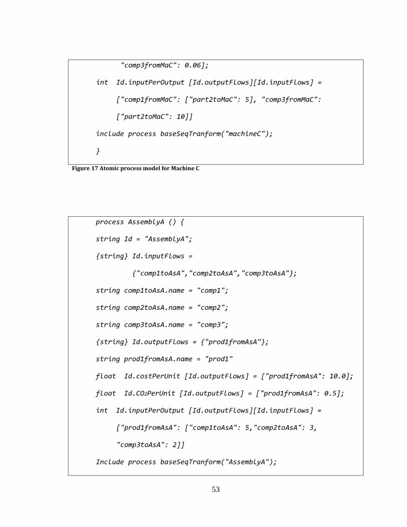
53

"comp3fromMaC": 0.06];


["comp1fromMaC": ["part2toMaC": 5], "comp3fromMaC":

["part2toMaC": 10]]

include process baseSeqTranform("machineC");

}

Figure 17 Atomic process model for Machine C

process AssemblyA () {

string Id = "AssemblyA";

{string} Id.inputFlows =

{"comp1toAsA","comp2toAsA","comp3toAsA"};

string comp1toAsA.name = "comp1";



{string} Id.outputFlows = {"prod1fromAsA"};

string prod1fromAsA.name = "prod1"

float Id.costPerUnit [Id.outputFlows] = ["prod1fromAsA": 10.0];

float Id.CO2PerUnit [Id.outputFlows] = ["prod1fromAsA": 0.5];


["prod1fromAsA": ["comp1toAsA": 5,"comp2toAsA": 3,

"comp3toAsA": 2]]

Include process baseSeqTranform("AssemblyA");

54

}

Figure 18 Atomic process model for Assembly A

process AssemblyB () {

string Id = "AssemblyB";

{string} Id.inputFlows = {"comp2toAsB","comp3toAsB"};

string comp2toAsB.name = "comp2";

string comp3toAsB.name = "comp3";

{string} Id.outputFlows = {"prod2fromAsB"};

string prod2fromAsB.name = "prod2";

float Id.costPerUnit [Id.outputFlows] = ["prod2fromAsB": 10.0];

float Id.CO2PerUnit [Id.outputFlows] = ["prod2fromAsB": 0.2];


["prod2fromAsB": ["comp2toAsB": 1, "comp3toAsB": 2]]

Include process baseSeqTranform("AssemblyB");

}

Figure 19 Atomic process model for Assembly B

Depicted in Figure 20 is a generic process composer model, which includes all flow

models and all sub-processes models, and formulates the flow aggregator models

automatically instead of being given explicitly. Again, three dots indicate that the input

and output flows, and sub-processes need to be instantiated before this generic model is

called. For every flow, the model needs to be included and its model name, matchName,

55

and aggregator name need to be defined before this generic model is called.

flowsToAggregators, a set of strings, are the union of input flows to the composite

process and output flows from all sub-processes. flowsFromAggregators, another set of

strings, are the union of all input flows to all sub-processes. All aggregator flow names

are in the set of strings that include all matchName of the flows. For every flow

matchName, if the name of input flow is in the flowsToAggregators and the name of the

output flow is in the flowsFromAggregators, then include the flow aggregator model with

the flow’s matchName as a parameter.

process processComposer(id) {



{string} Id.subProcesses = …;

{string} Id.flows = Id.inputFlows union Id.outputFlows;

for (f in Id.flows) {

string f.model = ...;

include flow f.model(f);

string f.matchName = ...;

string f.aggrModel = ...;

};

for (p in Id.subProcesses) {

string p.model = ...;

include process p.model(p);

56

}

{string} Id.flowsToAggregators =

Id.inputFlows union union(p in Id.subProcesses) p.outputFlows;

{string} Id.flowsFromAggregators =

Id.outputFlows union union(p in Id.subProcesses) p.inputFlows;

{string} Id.allFlows =

Id.flowsToAggregators union Id.flowsFromAggregators;

{string} Id.matchNames =

distinct({f.matchName | f in Id.allFlows});

for (n in Id.matchNames) {string Id.n.aggrModel =

first({f.aggrModel |f in Id.allFlows : f.matchName == n});

{string} Id.n.inputFlows = {

f | f in Id.flowsToAggregators : f.matchName == n};

{string} Id.n.outputFlows = {

f | f in Id.flowsFromAggregators : f.matchName == n};

include flow aggregator Id.n.aggrModel(Id.n);

};

Figure 20 Generic composite process model

Figure 21 shows the metrics aggregator models that compute daily total cost and CO2.

The daily total cost and CO2 are the sum of cost and CO2 for all sub-processes.

metric aggregator costSequence(Id) {

57

include context timeSequence ();

{string} Id.subProcesses = ...;

float Id.cost[t in timeSequence] =

sum(p in Id.subProcesses) p.cost[t];

}

metric aggregator CO2Sequence(Id) {

include context timeSequence ();

{string} Id.subProcesses = ...;

float Id.CO2[t in timeSequence] =

sum(p in Id.subProcesses) p.CO2[t];

}

Figure 21 Metric aggregator model

Figure 22 shows the composite process model. Model Id is twoProductsManuf. It

includes the context model itemSequence (). Id.inputFlows is given as a set of two strings

{“part1in”, “part2in”}. Id.outputFlows is given as a set of two strings of {“product1”,

“product2”}. matchNames are also given. Id.subProcessess is instantiated as a set of five

strings of {“machineA”, “machineB”, “machineC”, “assemblyA”, “assemblyB”}. The

generic process model processComposer is called to include all atomic sub-processes

models defined previously. Float type of data for extra facility cost and CO2 per day

($1750 and 0.3 metric tons) are provided. The metric aggregator models,

58

costSequence(Id) and CO2Sequence(Id), are included. Total cost for each day is the extra

facility cost plus daily cost for all sub-processes. Total CO2 for each day is the extra

facility CO2 plus total sub-processes CO2.

An alternative modeling method is to explicitly instantiate all flows and flow

aggregators, e.g., inputs and outputs of Part1, Part2, Comp1, Comp2, and Comp3 are all

specified as sets of strings. Then every flow aggregator is included with its name as a

parameter.

process twoProductsManuf () {

string Id = “twoProductsManuf”;


{string} Id.inputFlows = {“part1in”, “part2in”};

{string} Id.outputFlows = {“product1”, “product2”};

string part1in.matchName = "part1";

string part2in.matchName = "part2";

string product1.matchName = "product1";

string product2.matchName = "product2";


for (f in Id.flows) f.model = "itemSequence";

{string} Id.subProcessess = {

"machineA", "machineB", "machineC","assemblyA", “assemblyB"};

for (p in Id.subProcesses) p.model = p;

include process processComposer(Id);

59

float Id.extraCostSequence[t in timeSequence] = 1750.0;

float Id.extraCO2Sequence[t in timeSequence]= 0.3;

include metric aggregator costSequence(Id);

include metric aggregator CO2Sequence(Id);

float Id.totalCost =

sum(t in timeSequence)(Id.cost[t] + Id.extraCostSequence[t]);

float Id.totalCO2 =

sum(t in timeSequence)(Id.cost[t] + Id.extraCO2Sequence[t]);

}

Figure 22 Composite process model for the two-product-manufacturing process

All the SPDA model components for the example have been explained. Now we need to

exam the data required by the queries in Figure 9 and Figure 10. A context data sequence

is shown in Figure 23. Its product demand data model is listed in Figure 24, in which the

quantities of the two products are given for each production day. For example, [<4, 9,

2012>: 6] in the first line means demand for Product 1 on September 4, 2012 is 6.

{day} timeSequence = {

<4, 9, 2012>, <5, 9, 2012>,

<6, 9, 2012>, <7, 9, 2012>, <8, 9, 2012>,

60

}

Figure 23 A context data sequence for the two-product-manufacturing process

int product1.qty [timeSequence] = [<4, 9, 2012>: 6, <5, 9, 2012>: 8,

<6, 9, 2012>: 5, <7, 9, 2012>: 7, <8, 9, 2012>: 4];

int product2.qty [timeSequence] = [<4, 9, 2012>: 5, <5, 9, 2012>: 6,

<6, 9, 2012>: 3, <7, 9, 2012>: 4, <8, 9, 2012>: 5];

Figure 24 Product demand data model for product 1 and product 2

A what-if scenario for the example is described as follows: if the process engineer uses a

predefined production plan, i.e., all the data such as numbers of Part 1 and Part 2,

numbers of components flows into and out of Machine A, Machine B, Machine C, and

number of components flows into Assembly A, and Assembly B each day are fixed. This

means that all the data needed in the SPDA model are explicitly given, expressions can

be computed using these data. The four line of what-if query can be expanded as in

Figure 25. The constraint is the same.

{day} timeSequence = { <5, 11, 2012>, <6, 11, 2012>, <7, 11, 2012>, <8,

11, 2012>, <9, 11, 2012>, }

int product1.qty [timeSequence] = [6, 8, 5, 7, 4];

int product2.qty [timeSequence] = [5, 6, 3, 4, 5];

61

// data for fixed production plan

int part1.qty [timeSequence] = [ 98, 128, 73, 107, 56];

int part2.qty [timeSequence] = [127, 166, 96, 139, 221];

int part1ToMaA.qty [timeSequence] = [0, 0, 4, 0, 0];

int part2ToMaA.qty [timeSequence] = [0, 0, 0, 0, 0];

int part1ToMaB.qty [timeSequence] = [98, 128, 69, 107, 56];

int part2ToMaB.qty [timeSequence] = [127, 166, 96, 139, 61];

int part2ToMaC.qty [timeSequence] = [0, 0, 0, 0, 160];

int comp1FromMaA.qty [timeSequence] = [0, 0, 0, 0, 0];

int comp2FromMaA.qty [timeSequencetimeSequence] = [0, 0, 4, 0, 0];

int comp1FromMaB.qty [timeSequence] = [30, 40, 25, 35, 20];



int comp1FromMaC.qty [timeSequence] = [0, 0, 0, 0, 0];

int comp3FromMaC.qty [timeSequence] = [0, 0, 0, 0, 16];

int comp1ToAsA.qty [timeSequence] = [30, 40, 25, 35, 20];



int comp2ToAsB.qty [timeSequence] = [5, 6, 3, 4, 5];

int comp3ToAsB.qty [timeSequence] = [10, 12, 6, 8, 10];



Figure 25 What-if query for the two-product-manufacturing example

62

This is a deterministic computational model, however, since there is a constraint

statement in the query and there are also other data integrity constraints within the

composite process model and its sub-process models. The answers have to satisfy all the

constraints. The results of what-if scenario are: the total cost is $30,000 with a total of

35.11 metric tons of CO2. Note that changes in any input data will result a different set of

solutions.

For the optimization query listed in Figure 10, input data such as weekly

production schedule and customers’ demand for Product 1 and Product 2 are provided. A

sustainability goal is to determine an optimal production plan that minimizes the total

cost within a CO2 bound of 50 metric tons. The optimization model performs multiple

non-deterministic computations, each instantiates decision variables (quantities of flows

in each configuration) using values that satisfy all the constraints. Among those sets of

configurations that satisfy all the constraints, the system will automatically find a

configuration (i.e., a production plan) that minimizes the total cost. Figure 26 shows the

optimization result screen of an implementation using IBM ILOG CPLEX. The optimal

production plan for the scheduled five days is derived. The optimization results show that

the minimal total cost is $28,023 with total 36.72 metric tons of CO2. The results also

indicate that due to the higher operation cost of the Machine B, it is not recommended to

use Machine B to produce any of the components, i.e., Comp1, Comp2, and Comp3. Note

that changes in any of the input data and constraints will also affect the values of decision

variables and decision expressions.

63

Figure 26 Optimal solution screen of two-product-manufacturing example

3.4 SPDA Syntax and Semantics In this section, the syntax and formal semantics of SPDA will be presented. The SPDA

formalism includes two major parts; (1) Generic Analytics Language – represents generic

64

analytics knowledge and (2) Process Description and Sustainability Metrics - supports

sustainable process modeling and sustainability metrics computation.

Figure 27 presents the generic part of the SPDA formalism. The components are

explained as follows:

Analytical statements may be assignments, constraints, or decision variable

declarations.

An analytical sequence is simply a sequence of analytical statements. As classified in

section 3.2, there are five layers of abstraction in SPDA analytical sequences, namely

explicit, implicit, constraints, alternatives, and optimization layers.

An analytical model is an analytical sequence with the model name and a possible

parameter Id.

A model package is a set of SPDA models.

An SPDA query is a pair of an analytical sequence and a model package that includes

all models that are referred to, directly or indirectly, from the process model.

65

Analytical sequence

Analytical statement

Assignment statement Constraint statement Variable declaration statement

1

1..*

Model package Analytical model

1 1..*

Include statement

Analytical query10..* has

Implicit analytical sequence

Explicit analytical sequence

Optimization analytical sequence

Alternatives analytical sequence

Constraint analytical sequence

Optimization statement

0..*

1

has

1

1

has

Figure 27 SPDA formalism class diagram – generic analytics language

Figure 28 shows a hierarchical diagram for the Process Description and Sustainability

Metrics part of the SPDA formalism. The Process Description and Sustainability Metrics

part includes syntax of the SPDA analytical models such as process model, flow model,

flow aggregator model, and context model. These analytical models must adhere to a

more specialized structure, i.e., these models must have specific analytical statements as

shown in the two-product-manufacturing example.

Figure 27 and Figure 28 are connected through analytical model. An analytical

model can be models of process, context, flow, flow aggregator, or sustainability metric

aggregator.

66

Figure 28 A hierarchical diagram for the Process Description and Sustainability Metrics

A process model may be a generic process model or a specific process model. A generic

process model can be stored in a model library and reused for developing specific process

models. Flow and flow aggregator models may be those for discrete flows, continuous

flows, or time-based flows. Sustainability metric aggregator models are specifically

designed for sustainability metric aggregation for environmental indicators such as

energy, emission, material, and waste and economic indicators such as investment,

revenue, cost, and return on investment (ROI).

The SPDA library collects model components of both generic model and specific

model. Metrics model components can also be stored in a library. Figure 29 shows

examples of generic model components in the SPDA library, e.g., process model

components such as baseSeqTransform and baseProcessComposer, and flow and flow

67

aggregator models for discrete and continuous flows, and metrics models for

environmental and economic indicators. Figure 30 lists examples of specific model

components in the library; these models were developed for the two-product-

manufacturing example. In this case, it includes specific process models for machine A,

machine B, machine C, assembly A, assembly B, and composite model twoProdManuf for

the overall process. The model components in the SPDA library provide reusable

building blocks and can be used as templates for a family of manufacturing processes;

each model or template can be reused with some adjustment for different cases within the

family. New models can be added to the SPDA library. Moreover, the existing models

within the library can be executed with new data so that different companies that have the

same problems could use the models by inputting their data to seek company-specific

decision guidance. Using model components in the library, modelers can create SPDA

models and queries for their operations more effectively and efficiently.

68

Figure 29 SPDA component library: example of generic models

Figure 30 SPDA component library: examples of specific models

generic models

process models

baseSeqTransform

baseProcessComposer

flow and aggregator models

itemSequence

flowSequence

item

flow

metric models

costSequence

energySequence

wasteSequence

emissionSequence

context models timeSequence

specific models

machineA

machineB

machineC

assemblyA

assemblyB

twoProdManuf

69

SPDA model syntax: the OPL data model and the basic OPL syntax of arithmetic and

query expressions are adopted with minor modifications and extensions. Basic OPL data

model, modeling concept, data type, and data structure are listed in (IBM, 2012).

Analytical sequence, Aseq, is a sequence (s1, ..., sn) of analytical statements, si,,

1 ≤ i ≤ n, in one of the forms:

Ti xi = ai

Ti xi = ei

Ti xi

Ti xi = …

Ci

include Mi (J) or include Mi ( )

min xi , max xi , or sat

where:

The statements min xi , max xi , or sat are only allowed as the last statement sn

Ti is a type

xi is a variable name, which may include a prefix identifier, e.g., Id.x.

ai is a constant of type Ti

ei is an expression returning type Ti

“…” is a keyword in “Ti xi = …” to indicate that xi is to be instantiated with a

constant before using it later in the sequence

Ci is a constraint

Mi is a unique name of an analytical model

70

J in Mi (J) is a string identifier

The first four forms are declaration statements, within which the first two forms are

assignment statements. Ci is a constraint statement, include Mi is an include statement,

and min xi, max xi, or sat are optimization statements, i.e., minimization, maximization,

and satisfiability. If the last statement sn of the analytical sequence (s1, ..., sn) is min xi,

max xi, or sat, then the (s1, ..., sn) is an optimization analytical sequence; otherwise, we

say that it is a non-optimization analytical sequence.

An analytical model is an expression of the form

M(Id) { Aseq } or M( ) { Aseq }

where M is a unique name of the model, Id is an optional parameter, and Aseq is a non-

optimization analytical sequence.

Let P be a set of analytical models. We say that P is closed under reference (or

closed) with respect to an analytical sequence A (or model M) if the following holds: If A

has a statement of the form include M’(J), then P must contain an analytical model M’.

We say that P is closed under reference (or closed) if for every model M in P, P is closed

with respect to M.

An analytical query is a pair (A, P), where A is an analytical sequence and P is a

model package closed with respect to A.

Let (A, P) be an analytical query. The flattened sequence of A, denoted flat (A, P),

is an analytical sequence that results from A by recursively replacing each include M( )

with the analytical sequence of the model M ( ), and replacing each include M(J)

71

statement with the analytical sequence of the model M(Id) in P, in which every

appearance of Id is replaced with J.

We say that an analytical query (A, P) has a conflict, if one of the following holds

in

flat (A, P) = (S1,…, Si ,…, Sj,…, Sn):

Sj is a declaration statement of the form Ti xi = ai or Ti xi = ei and Si is any

declaration statement

Si and Sj are two declaration statements such that xi = xj and Ti ≠ Tj (i.e., the same

variable is declared twice with conflicting types)

Given a flat (S1,…, Si ,…, Sn) analytical sequence A (i.e., without include statement), we

say that variable xi is data-instantiated if:

There is a statement Si of the form Ti xi = ai , where ai is a constant or, recursively,

There is a statement Si of the form Ti xi = ei, such that all variables y in ei are

instantiated in the prefix sequence (S1,…,Si-1 )

We say that a flat analytical sequence A is data instantiated if every variable x in a

declaration statement is instantiated.

We say that an analytical query (A, P) is well-formed if:

It does not have a conflict, and

For every constraint statement Ci and expression ei in the declaration statement of the

form Ti xi = ei or min xi, max xi, or sat in flat (A, P), the following holds: it only

contains variables that have been declared in a declaration statement earlier in the

sequence.

72

If A is a non-optimization sequence, then, flat (A, P) must be data instantiated.

If A is an optimization sequence, then for every statement Si in flat (A, P) = (s1, ..., sn)

of the form Ti xi = …, xi must be instantiated in (S1,…, Si-1 ) (i.e., earlier in the

sequence).

From now on, only well-formed analytical queries are considered.

As discussed earlier, an SPDA model is an analytical model M (Id) if it is one of

the following forms:

Process model

Context model

Flow model

Flow aggregator model

Sustainability metric aggregator model

An SPDA process model with identifier Id, denoted PM (Id), is an analytical sequence

that contains statements of the following forms:

string Id.processType = type_flow_string,

{string} Id.inputFlow = inputFlowExpr,

{string} Id.outputFlow = outputFlowExpr,

{string} Id.subProcess = subProcessExpr,

{string} Id.flowAggregator = flowAggrExpr,

and

include M (I), for every I in Id.inputFlow, Id.outputFlow, Id.subProcess, or

Id.flowAggregator, where:

73

Id is used as a prefix for all variables on the left hand side of the declaration

statements, except for variables that appear on the left hand side of assignments into

variables defined in the included models, i.e., SPDA models M (Id’), where Id’ is in

Id.inputFlow, Id.outputFlow, Id.subProcess, and Id.flowAggregator (those are

“visible” to the process model)

type_process_string is a string

inputFlowExpr, outputFlowExpr are analytical expressions of the type {string} (i.e.,

return a set of strings)

subProcessIdsExpr, flowAggrIdsExpr are analytical expressions of type {string}

M (I) denotes a method that returns an SPDA model with identifier I

An SPDA context model CM ( ), is an analytical model.

An SPDA flow model with identifier Id, denoted FM (Id), is an analytical model

that contains statements of all of the following forms:

string Id.flowType = type_flow_string,

where:

Id is used as a prefix for all variables on the left hand side of the assignment

statements

type_flow_string is a string

An SPDA flow aggregator model with identifier Id, denoted FAM (Id), is an analytical

sequence that contains all of the followings forms:

string Id.flowType = type_flow_string,

{string} Id.flows_to_aggr = inputFlowExpr,

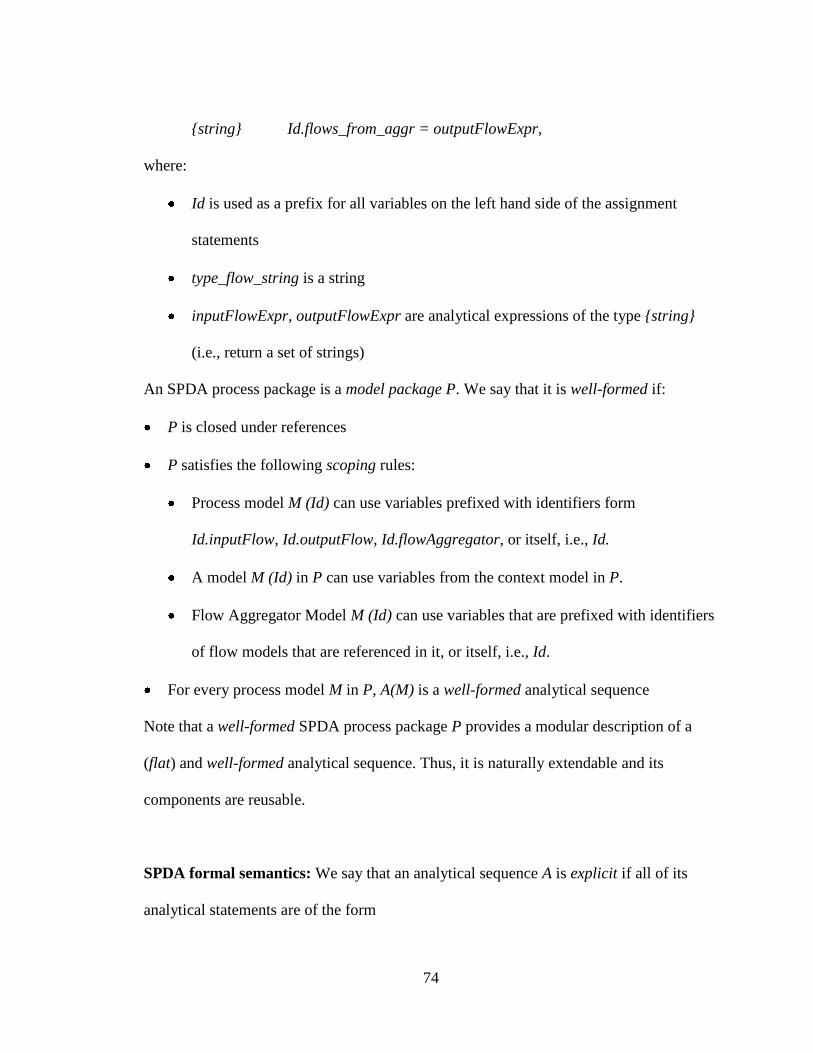
74

{string} Id.flows_from_aggr = outputFlowExpr,

where:

Id is used as a prefix for all variables on the left hand side of the assignment

statements

type_flow_string is a string

inputFlowExpr, outputFlowExpr are analytical expressions of the type {string}

(i.e., return a set of strings)

An SPDA process package is a model package P. We say that it is well-formed if:

P is closed under references

P satisfies the following scoping rules:

Process model M (Id) can use variables prefixed with identifiers form

Id.inputFlow, Id.outputFlow, Id.flowAggregator, or itself, i.e., Id.

A model M (Id) in P can use variables from the context model in P.

Flow Aggregator Model M (Id) can use variables that are prefixed with identifiers

of flow models that are referenced in it, or itself, i.e., Id.

For every process model M in P, A(M) is a well-formed analytical sequence

Note that a well-formed SPDA process package P provides a modular description of a

(flat) and well-formed analytical sequence. Thus, it is naturally extendable and its

components are reusable.

SPDA formal semantics: We say that an analytical sequence A is explicit if all of its

analytical statements are of the form

75

Ti xi = ai

where ai is a constant, i.e., it is an assignment of a constant to a variable. Intuitively, the

symbolic expression of an explicit analytical sequence represents the corresponding data.

Note that an explicit analytical sequence is flat. Formally, the semantics of an explicit

analytical sequence (s1, ..., sn), denoted Sem ((s1, ..., sn)), is itself, i.e., its symbolic

expression.

We say that an analytical sequence A is implicit if all of its analytical statements

are of the form

Ti xi = ei

Note that this includes the case when the expression ei is a constant ai. Formally, the

semantics of a well-formed implicit analytical sequence

(T1 x1 = e1, … , Tn xn = en)

is the explicit analytical sequence

(T1 x1 = a1, … , Tn xn = an)

in which each ai, 1 ≤ i ≤ n, is a constant of type Ti that is computed by expression ei,

when each variable xj, 1 ≤ j ≤ i-1, is replaced by the constant aj.

The semantics of (s1, ..., sn) is denoted Sem ((s1, ..., sn)). Obviously, an explicit

analytical sequence is a particular case of implicit, in which case, explicit and implicit

semantics coincide.

We say that an analytical sequence A = (s1, ..., sn) is a constraint analytical

sequence if all of its statements are of the form

(Ti xi = ei) or Ci

76

where ei is an expression of type Ti and Ci is a constraint. Formally, the semantics of a

well-formed constraint analytical sequence (s1, ..., sn), denoted Sem ((s1, ..., sn)), is defined

as follows:

Consider an implicit analytical sequence ( si1

,..., sik

), which is a sub-sequence of

(s1,..., sn) that contains all statements si’ of the form Ti xi = ei, and its semantics (Ti1

xi1

= ai1

,..., Tik xik

= aik

) (which is an explicit analytical sequence), and

Consider a sequence (C j1

, ..., C jm

), which is a sub-sequence of (s1, ..., sn) that

contains all the constraint statements

If there exists 1 ≤ i ≤ m, such that C ji

evaluates to FALSE after every variable xi

in it is replaced with the constant ai, then Sem ((s1, ..., sn)) is defined as INVALID.

Otherwise, Sem ((s1, ..., sn)) is defined as the explicit analytical sequence (Ti1 xi1

= ai1

,..., Tik xik

= aik

).

We say that an analytical sequence A = (s1, ..., sn) is an alternative analytical sequence, if

each si, 1 ≤ i ≤ n, is of the form

(Ti xi ), (Ti xi = ai), (Ti xi = ei), or Ci

where ai is a constant of type Ti, and ei is an expression of type Ti, and Ci is a constraint.

Note that an alternative analytical sequence may have repetition of declaration statements

for the same variable x. Consider the analytical sequence (s1, ..., sn) resulting from A by

removing, for every variable x, all declarations except for its first appearance in A.

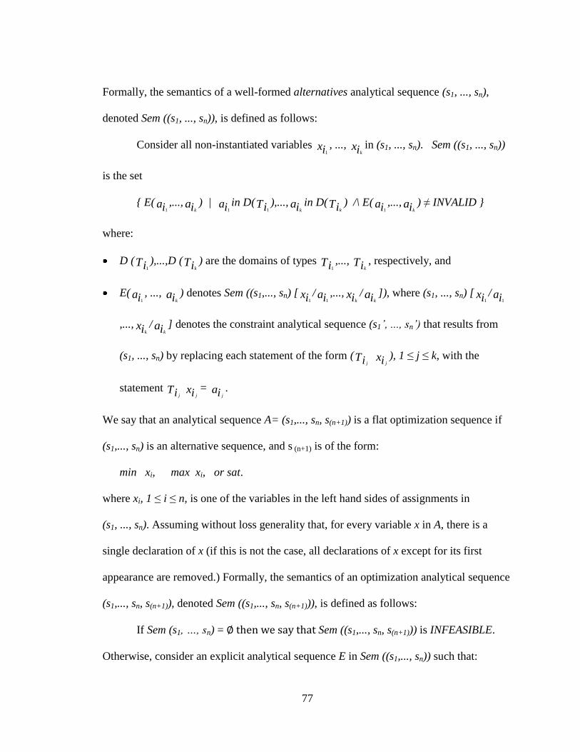
77

Formally, the semantics of a well-formed alternatives analytical sequence (s1, ..., sn),

denoted Sem ((s1, ..., sn)), is defined as follows:

Consider all non-instantiated variables xi1

, ..., xik

in (s1, ..., sn). Sem ((s1, ..., sn))

is the set

{ E( ai1

,..., aik

) | ai1

in D(Ti1

),..., aik

in D(Tik

) /\ E( ai1

,..., aik

) ≠ INVALID }

where:

D (Ti1

),...,D (Tik

) are the domains of types Ti1

,..., Tik

, respectively, and

E( ai1

, ..., aik

) denotes Sem ((s1,..., sn) [ xi1

/ ai1

,..., xik

/ aik

]), where (s1, ..., sn) [ xi1

/ ai1

,..., xik

/ aik

] denotes the constraint analytical sequence (s1’, ..., sn’) that results from

(s1, ..., sn) by replacing each statement of the form (Ti j xi j

), 1 ≤ j ≤ k, with the

statement Ti j xi j

= ai j

.

We say that an analytical sequence A= (s1,..., sn, s(n+1)) is a flat optimization sequence if

(s1,..., sn) is an alternative sequence, and s (n+1) is of the form:

min xi, max xi, or sat.

where xi, 1 ≤ i ≤ n, is one of the variables in the left hand sides of assignments in

(s1, ..., sn). Assuming without loss generality that, for every variable x in A, there is a

single declaration of x (if this is not the case, all declarations of x except for its first

appearance are removed.) Formally, the semantics of an optimization analytical sequence

(s1,..., sn, s(n+1)), denoted Sem ((s1,..., sn, s(n+1))), is defined as follows:

If Sem (s1, …, sn) = ∅ then we say that Sem ((s1,..., sn, s(n+1))) is INFEASIBLE.

Otherwise, consider an explicit analytical sequence E in Sem ((s1,..., sn)) such that:

78

If s (n+1) is min xi, then for all E’ in Sem ((s1, …, sn), ai ≤ ai’, where ai and ai’, are the

analytical model constants in the assignments Ti xi = ai of E, and Ti xi = ai’ of E’.

If s (n+1) is max xi, then for all E’ in Sem ((s1, ..., sn), ai ≥ ai’, where ai and ai’, are the

analytical model constants in the assignments Ti xi = ai of E, and Ti xi = ai’ of E’.

If E does not exist, we say that Sem ((s1,..., sn, s(n+1))) is UNBOUNDED. Otherwise,

Sem ((s1,..., sn, s(n+1))) is E.

Note that if s (n+1) is sat, the semantics is just an explicit analytical sequence E in

Sem ((s1, ..., sn)). Also note that the optimization semantics (whether it is minimization,

maximization, or satisfiability) are non-deterministic, i.e., there may be more than one

explicit model that satisfies the condition in the definition of semantics.

Consider the five layers (types) of analytical sequences (1) explicit, (2) implicit,

(3) constraints, (4) alternatives, and (5) optimization. Let L (1), L (2), L (3), L (4), and L

(5) denote sets of analytical sequences that can be expressed by each layer, respectively.

We claim that

L (1) L (2) L (3) {L (4)} L (5)

In addition, that the semantics of each layer are consistent with all lower layers. That is,

for any two layers i, j, 1 ≤ i < j ≤ 5, i ≠ 4, j ≠ 4’, if an AM A is in L (i), then Sem (i) of

A is also Sem (j) of A.

Semantics of a query (A, P) is a pair (A’, P’) constructed as follows:

For every sequence S, either A or a sequence B in a model M (Id) {B} in P, S is

replaced by S’ as follows.

Consider all variables x1, …, xn, declared in their order in S, then S’ is the sequence

79

(T1 x1 = a1 , …, Tn xn = an)

where T1 ,…, Tn are the corresponding types of x1, …, xn respectively, and ai is the

constant instantiated with xi in the semantics E of flat (A,P).

3.5 SPDA Query Computation In this section, algorithms (reduction procedures) to perform SPDA analytical query

computation are introduced. Figure 31 shows a commutative diagram for analytical query

computation, in which the upper left box indicates the query sequence A in model

package P. The query sequence may have include statements . The semantics of A is

sequence A’ in package P’ as shown in the upper right box in Figure 31. Two algorithms

are included in the computation – analytical query algorithm and flat optimization

sequence algorithm. Through the analytical query algorithm (refer to step (1), (6), and

(5)), (A, P) can be translated to a flat analytical sequence (middle left box). If the flat

analytical sequence can be instantiated, it is an implicit analytical sequence, otherwise, it

is an optimization analytical sequence whose semantics is a flat explicit analytical

sequence (middle right box). This algorithm calls the flat optimization sequence

algorithm (refer to step (2), (3), and (4)) to translate the flat optimization sequence to a

standard optimization model such as OPL or AMPL (lower left box). By using an

optimization solver, the optimization solution (lower right box) can be derived. All

variables can then be instantiated, the sequence becomes a flat explicit analytical

sequence (middle right box), which can be translate back to (A’, P’).

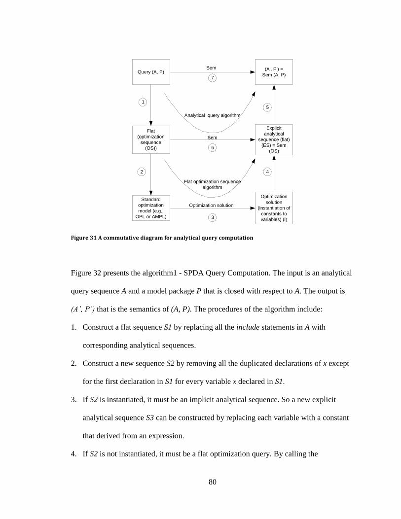
80

Query (A, P)(A', P') =

Sem (A, P)

Flat

(optimization

sequence

(OS))

Optimization

solution

(instantiation of

constants to

variables) (I)

Explicit

analytical

sequence (flat)

(ES) = Sem

(OS)

Standard

optimization

model (e.g.,

OPL or AMPL)

1

3

4

5

2

7

6

Sem

Sem

Optimization solution

Flat optimization sequence

algorithm

Analytical query algorithm

Figure 31 A commutative diagram for analytical query computation

Figure 32 presents the algorithm1 - SPDA Query Computation. The input is an analytical

query sequence A and a model package P that is closed with respect to A. The output is

(A’, P’) that is the semantics of (A, P). The procedures of the algorithm include:

1. Construct a flat sequence S1 by replacing all the include statements in A with

corresponding analytical sequences.

2. Construct a new sequence S2 by removing all the duplicated declarations of x except

for the first declaration in S1 for every variable x declared in S1.

3. If S2 is instantiated, it must be an implicit analytical sequence. So a new explicit

analytical sequence S3 can be constructed by replacing each variable with a constant

that derived from an expression.

4. If S2 is not instantiated, it must be a flat optimization query. By calling the

81

OptSeqAlg (S2) algorithm, it will return the semantics of S2.

Input: (A, P) is a well-formed analytical query and P is a closed form

model package closed with respect to A.

Output: (A’, P’) is the semantics of (A, P).

1. Construct S1 = flat (A, P).

2. Construct sequence S2 from S1 as follows:

For every variable x declared in S1, remove all declarations of x

except for the first declaration in S1.

3. Check if S2 is instantiated.

4. If S2 is instantiated, it must be an implicit analytical sequence of

the form (T1 x1 = e1, …,Tn xn = en). In this case, construct S3 as the

explicit analytical sequence (T1 x1 = a1,…,Tn xn = an),in which each

ai, 1≤ i ≤ n, is a constant of type Ti that is computed by expression

ei, where each variable xj, 1≤ j ≤ i-1, is replaced by aj.

5. Otherwise, if S2 is not instantiated, it must be a flat optimization

query. Construct S3 by calling the method OptSeqAlg (S2), which

returns the semantics of S2.

6. Construct the pair (A’, P’) as follows:

For every sequence S, which is either A or a sequence B in a

model(Id){B} in P, S is replaced by S’ as follows.

Consider all variables x1, …, xn, declared in their order in S, then S’

is the sequence (T1 x1 = a1,…,Tn xn = an) where T1,… ,Tn are the

82

corresponding types of x1, …, xn respectively, and ai is the constant

to instantiate xi in S3.

Figure 32 Algorithm 1: SPDA query computation

Figure 33 presents the algorithm 2 - Optimization Sequence Algorithm (OptSeqAlg). The

input is a flat optimization query S2 generated by the SPDA Query Computation

algorithm. The output is the semantics of S2.

1. For all variables that are instantiated in every statement, replace the expression with

the computed constant.

2. Construct decision variables that are not being instantiated.

3. Construct a set of constraints by replacing decision variables in every statement with

its constant. For any variable that is non-instantiated, a constraint is added.

4. Construct the optimization problem with objectives and constraints.

5. Solve the optimization problem using an optimization solver

6. Construct the answer sequence by removing all constraint statements and replacing

all the variables using constants computed or the optimization solutions.

Input: Flat optimization query (i.e., (s1,…,sn,s(n+1)) where sn+1 is of the

form min xi , max xi (1 ≤ i ≤ n) or sat where xi is not

instantiated on (s1, …, sn)).

Output: Semantics of (s1,…,sn,s(n+1)).

83

1. Consider all variables xi1

, ..., xim

in (s1, ..., sn) that are

instantiated. For every statement Si j

, 1 ≤ j ≤ k, of the form

Ti j xi j

= ei j

, compute ei j

, and replace ei j

with the computed constant

ai j

, i.e., resulting in Ti j xi j

= ai j

2. Construct the set of decision variable V to be the set of all non-

instantiated variables xl1

, ..., xlm

in (s1, ..., sn) ranging over the

domains corresponding to types Tl1

,…, Tlm

respectively.

3. Construct the set of constraints C as follows:

3.1 Initially, C = ∅.

3.2 For every statement si, 1≤ i ≤ n of the form Ci, add to C the

constraint resulting from Ci by replacing every instantiated

variable xi j

with its constant ai j

from Step 1.

3.3 For every statement Si of the form Ti xi = ei, where xi is non-

instantiated, add the constraint xi == ei’, where ei’ result from

ei by replacing each decision variable xi j

in ei with its constant

ai j

from Step 1.

4. Construct the optimization problem O;

V

min xn subject to C, V

max xn subject to C, or V

sat C according to s(n+1).

5. Solve the optimization problem O.

6. If O is infeasible, return “INFEASIBLE”, else if O is unbounded,

return “UNBOUNDED”.

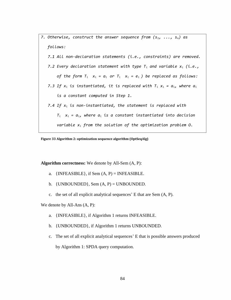
84

7. Otherwise, construct the answer sequence from (s1, ..., sn) as

follows:

7.1 All non-declaration statements (i.e., constraints) are removed.

7.2 Every declaration statement with type Ti and variable xi (i.e.,

of the form Ti xi = ai or Ti xi = ei ) be replaced as follows:

7.3 If xi is instantiated, it is replaced with Ti xi = ai, where ai

is a constant computed in Step 1.

7.4 If xi is non-instantiated, the statement is replaced with

Ti xi = ai, where ai is a constant instantiated into decision

variable xi from the solution of the optimization problem O.

Figure 33 Algorithm 2: optimization sequence algorithm (OptSeqAlg)

Algorithm correctness: We denote by All-Sem (A, P):

a. {INFEASIBLE}, if Sem (A, P) = INFEASIBLE.

b. {UNBOUNDED}, Sem (A, P) = UNBOUNDED.

c. the set of all explicit analytical sequences’ E that are Sem (A, P).

We denote by All-Ans (A, P):

a. {INFEASIBLE}, if Algorithm 1 returns INFEASIBLE.

b. {UNBOUNDED}, if Algorithm 1 returns UNBOUNDED.

c. The set of all explicit analytical sequences’ E that is possible answers produced

by Algorithm 1: SPDA query computation.

85

Claim: Algorithm SPDA query computation is CORRECT, i.e., it is:

1. Sound, i.e., for every well-formed analytical query (A, P),

All_Ans (A, P) ⊆ All_Sem (A, P)

2. Complete, i.e., for every well-formed analytical query (A, P),

All_Sem (A, P) ⊆ All_Ans (A, P)

Proof: See Appendix A for proof.

3.6 SPDA Features Summary After the development of SPDA, the last column of Table 1 is replaced by the SPDA

formalism (see Table 2). It shows the comparison of SPDA with other modeling

languages contrasting the same set of desirable features as in Table 1. Note that the SPDA

formalism supports data querying, what-if analysis, decision optimization, and unified

modeling for all these tasks. The modular design of SPDA formalism enables the built-in

process modeling and the creation of model library that in turn supports sustainability

metrics definition and reuse. Reuse makes it particularly easier for manufacturing and

business users to model composite processes, especially if there are graphical user

interfaces available.

Table 2 A comparison of SPDA with other languages contrasting desirable features Model

Languages

Features

Process

Description

Languages

(PSL,

BPMN,

SysML)

Database

Query

Languages

(SQL,

XQuery)

Simulation

Languages

(ARENA,

SIMAN, OO

languages)

Optimization

Modeling

Languages

(e.g., AMPL,

GAMS, OPL)

Optimization

Semantics

for OO and

Query

Lang’s

(CoJava,

DGQL)

SPDA

(Analytics

Language +

Process

Description

and

Sustainability

Metrics)

Data Not directly Yes Require AMPL and Yes Yes

86

manipulation

and querying

modeling and

programming

GAMS are not

designed for

query

processing;

OPL has some

built-in support

What-if

analysis

SysML-

parametric

diagram

Only for what

can be

expressed as

DB queries

Yes Mainly

designed for

optimization,

not what-if

analysis

Yes Yes

Optimization No Limited and

not efficient

Optimization

by simulation

approaches

can be added

Yes Yes Yes

Unified

modeling for

different tasks

No No No No Yes Yes

Built-in

support for

process

modeling and

sustainability

metrics

Process

modeling

and can be

extended to

support

sustainability

metrics

Can be

extended

Some support

it and others

may be built

on top

No No, but Can

be built on top

of CoJava

Yes with

components

library

Modular,

extensible,

and reusable

Yes Does not

support OO

extensibility

Yes Difficult to

reuse models

Yes for

CoJava – like

Java;

DGQL – just

like SQL

Yes with

components

library

Ease of use

(by

manufacturing

and business

users)

Can be easy

via graphical

interface

Relatively

easy (SQL

skills)

Programming

skills to

model

analytics;

Many allow

high-level

composition

functionality

Math/optimizati

on modeling

skills

CoJava

(programming

skills);

DGQL (SQL

skills)

Easy for

composite

process, esp. if

a graphical

interface is

added; similar

to OPL for

atomic process

models

87

4. METHODOLOGY

A high-level SM improvement methodology has been discussed to explain the context of

SPDA in section 3.1. In this section, a more detailed specific model based decision

guidance methodology that provides procedures and guidelines for systematic

sustainability analysis using the SPDA formalism is presented. Before the discussion of

the methodology, potential users of a decision guidance management system that applies

the methodology are introduced. Figure 34 shows the concept and users of such a system

that is based on the SPDA sustainable process knowledge representation and supports

easy, faster, and reliable decision making for real world problems.

User interface

SPDA analyst

Decision maker

SPDA knowledge base administrator

Queries

Recommendations

Answers

Build models

Create/maintainknowledge artifacts

Answers

SPDA Formalism

Decision Guidance Management System for

Sustainable Manufacturing

Figure 34 Concept of the decision guidance management system for sustainable manufacturing using the SPDA formalism

88

Most people within factory floor do not have the expertise to formulate and solve

optimization problems using MP or CP. The SPDA formalism makes the process analysis

modeling intuitive and straight forward for domain users (with some IT background) such

as manufacturing engineers and decision makers. Figure 35 shows a high-level use-case

model of an implementation for the decision guidance management system using the

SPDA formalism. Not all the interrelationships between use cases are shown in the

Figure, for example, building models is related to setting up objectives. There are three

types of potential users. Each type of user has different roles in using and/or maintaining

the system.

SPDA analyst: The analyst is a primary user of the system. S/he may be a process

engineer who is in charge of defining case scenarios, setting up analysis model

objectives together with decision makers, and identifying sustainability metrics,

constraints, and controls. S/he also collects data from the factory floor to represent

process structure, flow, and metrics using existing SPDA model components from the

SPDA library or creating SPDA models from scratch.

Decision maker: The decision maker is the end user of the system. S/he identifies the

SM objectives/goals, provides model requirements, and asks the query questions

discussed above. The decision maker queries the knowledge base, and asks what-if

analysis and/or optimization questions for a specific problem. S/he may also compose

SPDA models simply using model components in the SPDA library.

SPDA knowledge base administrator: The knowledge-base administrator is

responsible for updating system data, creating reusable knowledge artifacts and new

89

applications, maintaining the SPDA model library, modifying/improving the system

design, and maintaining/enhancing the system.

Figure 35 Use case for implementation of decision guidance management system using the SPDA formalism

Figure 36 shows the steps of the methodology that allows users of a decision guidance

management system to model and perform sustainability analysis and derive decision

recommendations. It involves identifying manufacturing process problem scenarios, in

which the sustainability performance need to be assessed and optimized; collecting

domain knowledge for the relevant indicators and their metrics of the scenario;

developing conceptual models of the manufacturing processes; collecting and processing

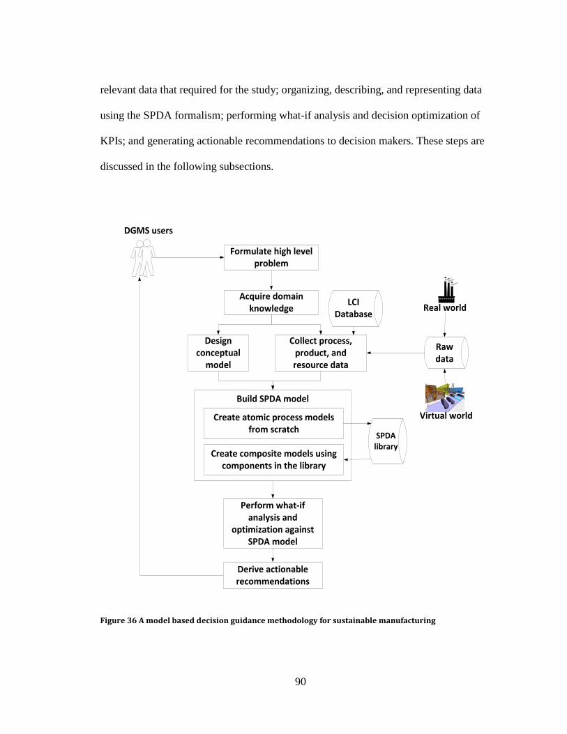
90

relevant data that required for the study; organizing, describing, and representing data

using the SPDA formalism; performing what-if analysis and decision optimization of

KPIs; and generating actionable recommendations to decision makers. These steps are

discussed in the following subsections.

Raw data

Formulate high level problem

Acquire domain knowledge

Design conceptual

model

Collect process, product, and resource data

Derive actionable recommendations

LCI Database

DGMS users

Perform what-if analysis and

optimization against SPDA model

Virtual world

Real world

Build SPDA model

Create atomic process models from scratch

Create composite models using components in the library

SPDA library

Figure 36 A model based decision guidance methodology for sustainable manufacturing

91

4.1 Formulation of High Level Problem More and more manufacturers consider sustainability in different aspects such as product

design, production and investment planning, branding, and corporate sustainability

objectives to satisfy multiple stakeholder requirements. They need to assess their

sustainability performance and take actions to improve it. To formulate a problem for

sustainability analysis using SPDA formalism, the decision maker(s) and SPDA

analyst(s) need to follow the steps to:

Identify or define a manufacturing process or a facility, e.g., two-product-

manufacturing-production line.

Define the objective(s) of the study, e.g., find out the best process plan that results

minimal energy consumption for producing a product.

Define the scope of the study including assumptions, conditions, and level of

abstractions for the problem.

Determine the types of information required for decision-making, e.g., the cutting

speed range for minimal negative environment impact.

Once the problem is identified or defined, the information and domain knowledge need to

be collected.

4.2 Acquisition of Domain Knowledge To model and analyze sustainability performance of manufacturing processes, both

traditional manufacturing knowledge and sustainability related information need to be

collected. As such, the modelers need to:

Understand the requirements of the problem under study, for example, for a

machining process, the requirements may include all aspects such as characterization

of the process, material, cutting tool, and finished parts; machining conditions; tool

92

requirements and tool paths; coolant and lubricant requirements; waste restrictions;

and energy used.

Identify KPIs, which may include both sustainability related indicators and

conventional indicators, e.g., energy and material efficiency, waste, emission, cost,

cycle time, throughput, and quality.

Identify the relationships among the indicators, e.g., equations that convert energy

units to equivalent carbon dioxide emissions.

Identify sustainability metrics, controls, and constraints, e.g., energy consumption as

a metric, machining time as a control variable, and spindle speed range as constraints.

Identify and define assessment formulas for required metrics computation, e.g., a

formula to calculate the emissions from a machining process.

Having knowledge is not enough; information needs to be related in a big picture to

prepare the analysis.

4.3 Design of Conceptual Model A conceptual model is a simplified representation of a real world problem. The

conceptual model provides the right level of abstraction that satisfies the modeling

objectives, and focuses on the metrics of concerns. It can be regarded as sketches of the

problem based on the knowledge collected; a conceptual model helps the modelers better

understand the problem and prepare for solutions. It is a necessary step for a modeler to

think, sort, and solve the problem. When designing a conceptual model, the answers to

the following typical questions for sustainability performance analysis need to be kept in

mind by the designers:

What are the processes or sub-processes need to be modeled?

93

What are the inputs and outputs of each process?

What are the relationships between processes?

What are the sustainability indicators?

What are the metrics of each indicator?

What are the data requirements?

What are the dependency relationships (e.g., correlations) among the indicators and

inputs?

The conceptual model provides requirements for data collection.

4.4 Collection of Data Data contents, units, and formats are specific requirements for model development and

execution. For example, LCA study involves data from Life Cycle Inventory (LCI)

databases, what-if analysis needs different sets of input data for computation and

comparison for alternatives, and optimization requires data for parameters of closed-form

mathematical expressions. Therefore, the sources of sustainability data need to be

identified first; it can be from LCI databases, real world, or virtual world. Then, what

data are available needs to be determined, for those data that are not available but

required, estimation or approximation are needed using various mathematical techniques

such as the Least-Squares estimation method (Brodsky, J. Luo, & Nash, 2008; Shao,

Brodsky, Ammann, & McLean, 2009). Data collected have to be converted to the correct

units in order to have meaningful results, for example, if second is used for time, all data

units for time need to be in seconds. The following subsections describe the different data

sources and data collecting methods (Shao, Bengtsson, & Johansson, 2010).

94

LCA methodology and LCI data: LCA is an effective methodology for sustainability

performance analysis of manufacturing processes. The LCA parameters include energy,

resources, waste, and emissions. LCA results provide information about the relative

impacts of different types of products, materials, as well as resource use and emissions

from different industry. For example, the environmental impact of producing an

automobile would include not only the impacts at the final assembly process, but also

those from mining metal ores, making electronic parts, forming windows, and any other

processes required for building a car (EPA LCA, 2010). LCI data support LCA. There are

two data streams in LCI: Primary data and secondary data. Primary data are derived

directly from manufacturing processes. Secondary data are data from databases or from

peer-reviewed literature. Primary data may be proprietary, hence may not be always

accessible. Currently, there are publicly available LCI databases for different regions. An

example of such a database is the European Commission Life Cycle Database (ELCD),

General-purpose LCA study can also use databases come with LCA tools such as

Ecoinvent, GaBi, and SimaPro (Stutz, 2010; Kent, 2007).

Real world data: Real world data can be collected from devices, machines,

manufacturing processes, production databases, or other engineering and manufacturing

application systems. For example, the sustainability data from the real world may be

extracted through the following protocols and systems:

95

MTConnect: MTConnect is a middleware standard that enables the data extraction

from machine tools using the eXtensible Markup Language (XML) standard.

MTConnect provides a mechanism for system monitoring, process, and optimization

with respect to energy and resources. The information is valuable for analyzing

sustainability performance of processes and facilities (Vijayaraghavan, Sobel, Fox,

Dornfeld, & Warndorf, 2008). Bengtsson et al. (2010) developed a case study using

MTConnect to acquire Boeing production data for modeling of sustainable

machining.

The Object Linking and Embedding for Process Control (OPC): OPC is a technique

for monitoring manufacturing systems and their status. It specifies the communication

of industrial process data, alarms and events, historical data, and batch process data

between sensors, meters, controllers, software application systems, and notification

devices (OPC, 2009).

Energy Management System (EMS): EMS is a system that monitors and collects

energy consumption data. The energy data can be mapped to logged data from other

sources such as Programmable Logic Controller (PLC) and OPC. For example, it can

be used to identify potential energy peak usage for certain operations within

manufacturing (Energy Management System, 2010).

Virtual world data: Virtual world data can be obtained from simulation systems,

engineering systems such as Computer Aided Design/Computer Aided Manufacturing

(CAD/CAM) systems, or Product Data Management (PDM) systems. For example:

96

SolidWorks Sustainability provides LCA on parts or assemblies within a design

window and compares materials for their environmental impact (NIST Workshop,

2010).

A machining simulation model can be developed to execute actual NC programs,

which describe tool path, cutting speed, and feed rate for producing a part. The

simulation result provides information regarding the energy consumed, material

required, and waste produced (Shao, Lee, & McLean, 2003) and other environmental

impact data (Shao, Kibira, & Lyons, 2010; Shao, Chernow, Kibira, & Lyons, 2011).

The domain knowledge and data collected provide information required for SPDA

modeling.

4.5 Building of SPDA models The formal syntax and semantics of SPDA have been presented in Section 3.4. In this

subsection, procedures for different users to model the problem using SPDA formalism

are discussed. By now, the users should have the knowledge to answer the following

questions:

How many processes need to be modeled?

Is a process a composite process or an atomic process?

What are the flows that flow into and out of the processes?

What are the objectives of the model?

What are the metrics need to be computed in each process?

What are the overall sustainability metrics for the composite process?

What are the explicit data, i.e., data are provided directly?

97

What are the implicit data, i.e., data are not directly available but can be computed?

What are the data types?

What are the data need to be determined (decision variable), e.g., data that can be

controlled by the users or instantiated by an optimization solver?

What are the constraints of the model, i.e., conditions need to be satisfied?

Procedures of SPDA modeling: According to the knowledge collected and conceptual

model of the problem, and the question just answered, users can develop modular SPDA

sub-models that include context models, flow models, flow aggregator models, atomic

process models, and sustainability metrics computational models. A composite process

model integrates sub-models by using include statements. As indicated in Figure 36, there

are two kinds of modeling scenarios:

1. If there is no appropriate model component in the SPDA library to adopt, modelers

need to create all components and composite SPDA models from scratch. This

requires the modelers to have more modeling knowledge or more training. These

model components can then be stored in a SPDA library for future use.

2. If there are appropriate model components available in the SPDA model library, the

modelers can create composite models by including the model components. It is

much easier than developing models from scratch. Note that the modelers need to

ensure that new data are reflected and modification might be needed. This type of

modelers might be decision makers who only require minimal training on SPDA

modeling.

98

The SPDA models have been defined and explained via an example in Section 3.3. The

general flowcharts of creating these typical SPDA models are shown in Figure 37

through Figure 42 respectively. These flowcharts are explained briefly as follows.

Figure 37 is the flowchart for creating a “context” model. Model name is defined

first and then data, which can be accessed by other related SPDA models, are declared.

Start

Context model

name

Context data

declaration

End

Figure 37 Context model flowchart

Figure 38 shows the flowchart for creating a flow model. The flow model has a parameter

Id, which is replaced by the actual parameter in an include statement that calls the flow

model. The context model is included. Data types and structures for the flow are

declared. Data constraints, if any, are defined in the model.

99

Start(parameter

Id)

Include context model

Declare data types and structures

End

Add constraints if any

Figure 38 Flow model flowchart

Figure 39 is the flowchart for creating a flow aggregator model. Again, parameter Id is

replaced by actual parameter in an include statement that calls the flow aggregator model.

The context model is also included. Id.inputFlows and Id.outputFlows are declared as a

set of strings and are instantiated separately. Id.flows, the union of Id.inputFlows and

Id.outputFlows, is also a set of strings. Data types and structures for the flows in Id.flows

are declared. Data constraints, if any, are also defined. Normally, one of the constraints is

100

that the total number (amount) of the inputFlows equals to total number (amount) of the

outputFlows.

Start(parameter

Id)


Declare data types and structures for input/

output flows

End


Figure 39 Flow aggregator model flowchart

Figure 40 is the flowchart for creating a generic atomic process model. The Id is provided

when it is called. For every flow, input flow or output flow, the flow model is included

with a parameter of the flow name. Metrics data type and structures are declared. Metrics

computations are expressed. Necessary constraints are also presented in the model.

101

Start(parameter

Id)


Declare data types and structures for input/

output flows

End

Include flow model

All flow models included?

Define metrics

Declare metrics data types and structures

No

Yes

Figure 40 Generic atomic model flowchart

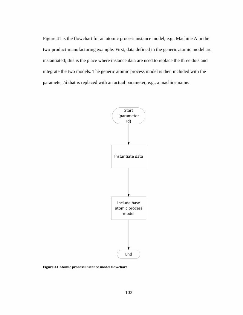
102

Figure 41 is the flowchart for an atomic process instance model, e.g., Machine A in the

two-product-manufacturing example. First, data defined in the generic atomic model are

instantiated; this is the place where instance data are used to replace the three dots and

integrate the two models. The generic atomic process model is then included with the

parameter Id that is replaced with an actual parameter, e.g., a machine name.

Start (parameter

Id)

Instantiate data

Include base atomic process

model

End

Figure 41 Atomic process instance model flowchart

103

Figure 42 is the flowchart for creating a composite process model. Model Id is replaced

when an SPDA query is formulated. It includes the context model. All the sub-processes

are declared and included by calling the atomic models with appropriate parameters.

Then, each flow and flow aggregator model are included. Finally, the computations of

total metrics are expressed. Sustainability metrics models are basically computational

model for specific problems. Once built, they can be stored in the model library for future

reuse.

By following these flowcharts, modular SPDA models such as context models,

flow models, flow aggregator models, atomic process models, and composite process

models can be incrementally developed without changing any of existing models or

queries. This is in contrast to the current common practice where the introduction of a

new component or factor leads to major redesign and reimplementation of the models and

associated algorithms for a decision optimization task.

104

Start (parameter

Id)


Declare sub-processes

End

Include sub-process model

All sub-processes included?

Define total metrics

No

Yes

Include flow and aggregator model

All included?

No

Yes

Figure 42 Composite process model flowchart

105

4.6 What-if analysis and Optimization Query using SPDA With all the required SPDA models developed, SPDA analytical query is ready to be

formulated. There are mainly two types of queries: What-if analysis query and decision

optimization query. Figure 43 is the flowchart for creating a SPDA query. First, data

required by the SPDA model are included. The final model of the composite process is

also included. Constraints, if any, are added. Finally, if it is an optimization query,

depending on the optimization objective, an optimization statement (minimize, maximize,

or satisfiability) need to be added. Note what-if analysis query does not have the final

step.

Include available data associated with the

SPDA models

Include final SPDA model

Add an optimization statement if it is a optimization query


Start

End

Figure 43 SPDA query model flowchart

106

Using a translator that implements the SPDA query computation algorithms, the

analytical query formulated by users can be translated to a standard optimization model

such as OPL model, which can be solved using an optimization solver. If the problem is

valid and feasible, an optimal solution will be provided as actionable recommendations to

decision makers. Figure 44 depicts these steps of solving an analytical query in a decision

guidance management system.

Figure 44 Steps for solving an SPDA query in a decision guidance management system

107

Then, what-if analysis or decision optimization against the SPDA query can be

performed. If the query can be translated to an explicit analytical sequence, all variables

in the expressions can be instantiated through computation using given data. What-if

analysis is a deterministic computational model that allows users to try a wide variety of

scenarios using the same model with different sets of input data such as historical

process, production, and sustainability data to predict different outcomes. Different

answers of what-if analysis allow decision makers to compare and assess changes before

they happen. For example, given certain settings of a process’ controls and input, the total

energy consumption, carbon emission, and costs can be predicted before investing on a

machine tool. In an optimization query, the optimization objectives are indicated using

minimize, maximize, or satisfiability statements. If data are not explicitly given, they will

be treated as decision variables, which will be instantiated by the optimization solver.

4.7 Actionable Recommendation SPDA models enable knowledge representation of manufacturing processes and compute

relevant sustainability metrics. A decision guidance management system that based on

SPDA models generates the SPDA query results, i.e., actionable recommendations for

SM improvement. The recommendations are from the two kinds of queries:

What-if analysis - query results from explicit data for different scenarios can be

computed and compared to select the most appropriate option.

Decision optimization - query results from decision optimization are the best

alternative that satisfies users’ objectives and constraints.

108

The systematic analysis and quantitative recommendations not only provide decision

makers with confidence, but also give the them flexibility to try different options, e.g., by

defining a new scenario or changing input data, sustainability objectives, or constraints.

109

5. CASE STUDIES

Case studies, using the SPDA formalism and the SM decision guidance methodology, can

be conducted to assess, analyze, and optimize the sustainability performance of

manufacturing processes, systems, and facilities. Such studies are designed to solve

decision optimization problems for answering specific questions through quantitative

analysis. Users can determine the material, labor, equipment, tooling, inventory, material

handling, and maintenance requirements according to the decision recommendations to

manage energy, emission, and waste systematically. In this section, two categories of

case studies are discussed, followed by two case studies, one from each of the two

categories.

5.1 Classification of potential SM case studies using SPDA

When classifying various SM case studies, different operational levels and their

abstractions and functional requirements have been considered. Sustainability data can be

aggregated for hierarchical production levels include supply chain level, factory level,

production line level, workstation level, equipment level, and process level (McLean &

Leong, 2002). Figure 45 shows an aggregation and decomposition of energy consumption

and CO2 emissions data for the hierarchical production levels.

110

Process

Equipment

Workstation

Production line

Factory

Supply Chain

En

erg

y c

on

su

mp

tio

n a

nd

CO

2 e

mis

sio

n

Figure 45 Aggregation of sustainability factors for hierarchical production levels

Optimization might be applied to different scenario at each hierarchical level for different

objectives and analysis requirements. For example, the evaluation of a company’s

business performance is a long-term strategic decision as opposed to the determination of

a daily production schedule, which is a short-term operational decision. Potential SPDA

case studies are classified according to the following two categories:

1. Decision guidance for investment/planning aspect of SM, i.e., solving problems

related to manufacturing planning and design.

2. Decision guidance for operational aspects of SM, i.e., solving problems related to

manufacturing operation and process.

The following subsections provide a sample list of possible case studies using SPDA in

these two categories.

111

Case studies for investment/planning of sustainable manufacturing: Because of the

complexity of manufacturing systems, processes, and related data measurement and

collection, decision-making for a long-term strategic planning is not a straightforward

process. The complex quantitative effect of factors of the cases needs to be analyzed. The

inputs and constraints for these cases may be factors such as regulatory policies,

production goal, enterprise profit, sales, budget, investment, and incentive. An initial set

of potential case studies from this aspect using SPDA modeling is identified based on

ideas from (McLean & Shao, 2003) (Kibira, Shao, & Lee, 2010) (Kibira & McLean,

2008). They are briefly listed below:

Economy: Model objectives may be determining the optimal investment allocation

for facility construction, technologies, materials, equipment, production, energy,

water, land, transportation, and labor. Model constraints may be total budget,

limitation of energy supply, level of material toxicity, cost of non-compliance, taxes,

and tradeoff between sustainable process costs, productivity, and maintenance cost.

Market Forecast: Model objectives may be predicting the future demand for products

based on historical economic and market data, and estimating the optimal production

levels to assist planning for the best production support strategies. Model constraints

may be energy consumption requirement for production, production capacity, and

transportation cost.

Supply Chain: Model objectives may be analyzing energy consumption for the entire

supply chain including warehousing and transportation network to minimize GHG

112

emissions, identifying the best route for transportation, and determining the optimal

lead times, cost, schedules, and inventory levels. Model constraints may be budget,

delivery date, and special customer requirement.

Facility Site Selection: Model objectives may be selecting the best site for optimal

sustainability performance of a new manufacturing factory. Model constraints may

include local real estate and energy costs, labor rate and availability, transportation

accessibility, climate conditions, and suitability of using renewable energy resources

such as solar or wind power.

Plant Layout: Model objectives may be determining the optimal floor space, lowest

energy consumption, and most efficient material handling route and buffer areas to

avoid bottlenecks and non-value-added activities. Model constraints may include

operational and maintenance accessibility requirements, material handling system

operational and safety requirements, and budget for new or change of plan.

Energy Demand Control: Model objectives may be reducing the energy cost by

analyzing options such as minimizing the use of energy during the peak demand

periods. Model constraints may include utility and curtailment contracts, production

energy requirements, cost of standby generators, and availability of renewable energy

sources.

Case studies for operational of sustainable manufacturing: Decision-making for SM

at different operational level can be performed in different ways, depending on the

objective. An initial set of potential case studies from this aspect using SPDA modeling is

113

identified based on the ideas from (McLean & Shao, 2003) (Kibira, Shao, & Lee, 2010)

(Kibira & McLean, 2008). Each study is briefly defined below:

Scheduling: Model objectives may be selecting the best scheduling algorithms that

lead to the lowest operational cost and highest productivity. Model constraints may

include number of shifts, shift schedules, resources availability, electricity peak

demand, and peak hours.

Planning and Control: Model objectives may be determining the minimal production

cost, shortest lead times, and the highest throughput. Model constraints may include

inventory location, size, and safe levels; and available resources (energy, material,

equipment, and labor).

Process Plan: Model objectives may be selecting the best manufacturing process plan,

determining the optimal combination of operational cost and energy efficiency, and

minimizing environmental impact by controlling energy consumption, carbon

emissions, use of hazardous substance, and noise. Model constraints may include

product design requirement, equipment/machine capabilities, and alternative energy

sources options.

Energy Management System: Model objectives may be determining the optimal

on/off schedule of lights and HVAC for production facility and offices based on the

occupied/unoccupied status to minimize production and HVAC system energy

consumption. Model constraints may be types and hours of operation, weather

conditions, and human comfort.

114

Sustainable Machining: Model objectives may be determining the optimal cutting

conditions to minimize energy consumption, material usage, waste, and CO2

emission; and optimal tool path. Model constraints may be budget for machine

purchase, machine capability, spindle speed range, and availability of tooling.

5.2 Case Study 1 - Investment/planning for Energy Efficient Manufacturing Manufacturers have been regarding energy as necessary cost of supporting production

and facility, that is why energy management has had a lower priority than production

management. However, the U.S. Energy Information Administration (EIA) expects

substantial increases in energy prices over the next two decades. “Manufacturers, who

don’t have much leeway when it comes to raising prices on their goods, will have to learn

to run factories on less energy or risk financial strain (Rockwell Automation, 2011).”

Because production cost is directly influenced by energy usage. Manufacturing process

optimization and energy management can help search for an optimal operating point that

is consistent with productivity, sustainability, and quality targets, and in line with cost

constraints, human comfort, and imposed environmental emission limits. Process

parameters that influence product quality, production capacity, energy consumption, and

emission levels need to be identified and manipulated using a systematic methodology.

There is a large range of energy management technologies (e.g., renewable energy

sources, standby generators, energy storage systems, and more efficient HVAC systems)

currently available. The deployment of these technologies within a factory is based on the

decisions on a mix of investments and operational strategy according to the

manufacturer’s sustainability goals and limitations; those decisions may involve

115

considerations of many complex interactions among different factors. For example, to

determine the optimal energy cost, renewable energy credits, savings, and ROI for a

particular investment option, a baseline of the current energy consumption and costs must

be computed first, and then the energy consumption and costs are assessed with

implementing new technologies, methodologies, and tools. The solution may involve

adding energy storage and local generation, and committing a higher level of curtailment

would result higher monetary rewards (Brodsky, Mana, Awad, & Egge, 2011). A new

configuration would also involve finding the best parameter settings, e.g., contractual

arrangement the manufacturer should make with electricity, gas, and water utilities, as

well as load curtailment companies.

Most industrial facilities have two types of electricity charges: energy cost, which

is measured as kilowatt-hours (kWh), and a peak demand cost, which is measured at

kilowatts (kW). Electricity costs differently at different times of the day. Peak demand is

a significant component in the cost of electricity in manufacturing industries. From a

company’s utility contract, the Tariff Rate Schedule (TRS) can be analyzed. Table 3 is an

example TRS table modified based on a table from (Mort, 2011). The demand cost is

$16.00 per kW; this means if the utility company measures the electricity usage every 15

minutes for the whole month, the peak energy use of the month is the demand and the

demand charge is the demand amount times $16.00 (i.e., every kW reduced from this

peak is worth $16.00). The facility energy manager needs to make wise decisions on peak

demand based on electric tariff rates, availability of local energy generation, and

116

incentives to curtail peak usage. Manufacturers can then schedule their equipment to run

during the periods of lower demand unless it is not possible.

Table 3 An example tariff table

Problem formulation: This case scenario, data, equations, and OPL code are mainly

adopted from (Brodsky, Ngan, Egge, & Backus, 2012). A factory power plant plans to

expand the existing energy equipment to meet the factory’s current and future energy

demand including electricity, heating, and cooling. Currently, the energy facility operates

a centralized heating and cooling plant (CHCP) system and utilizes the electricity

purchased from the local power company to satisfy all the energy demands. Due to the

growth of the factory, the existing CHCP system will not satisfy the future energy

demand and may require huge capital investment to expand the capacity and add new

technologies. Different configuration options have been proposed for the expansions.

This case study is to determine the best investment option that satisfies the current and

future demands at a minimal cost. This dissertation contributes the SPDA models

development using the SPDA formalism.

Time Period Energy Cost Unit

Peak Demand Load (1600 kW):

8 am to 8 pm Monday to Friday

$16 kW

On Peak : 8 am to 8pm Monday

to Friday

$ 0.08 kWh

Off-Peak: 8 pm to 8 am

Everyday

$0.06 kWh

117

Figure 46 shows the major components of the energy generation process to satisfy

the demand of electricity, heating, and cooling for the factory. The CHCP system

generates hot and cold water to meet the heating and cooling demands. Natural gas,

water, and electricity supplies are from local utility companies. To simplify the problem,

water supply (dashed line) has not been modeled in this case study. The GHG emissions,

such as the carbon dioxide (CO2), are also an important factor to aid decision-making.

Gas Supply Current Heating/Cooling

Plant

Electricity Supply

New CoGenPlant

Cost

CO2

Water Supply

Heat

Cool

Electricity

Figure 46 Prospective heating, cooling, and electric facilities diagram

The facility manager plan to deploy the best investment option that satisfying projected

demands and minimizing investment cost, maintenance expenditures, replacement

118

charges, operating expenses, and GHG emissions while maximizing savings and ROI.

One of the proposed options is to integrate a new cogeneration (CoGen) plant into the

existing facility as shown in Figure 46. The new CoGen plant has turbines to generate

electricity, uses the generated heat as a by-product to complement the heating demand,

and also supplies the cooling demand. An optimization model needs to be developed to

instantiate operational parameters and control variables that satisfy all the constraints.

The objective of the model is to find the optimal parameter settings for the interactions

between the existing and the newly added equipment. The annualized evaluation

parameters include:

investment cost (Ii),

the base investment cost (I0),

equipment cost (Ei), i.e., maintenance expenditure (Mi) plus replacement charge (Ri),

operating expense (Ci), i.e., the charges on electric and gas consumptions,

cost saving (Si),

ROI, and

the GHG emissions (Metric Tons of Carbon Dioxide Equivalent (MTCDEi)).

These parameters are evaluated against the various investment options. The comparison

results enable facility managers to determine the best investment option out of all of the

options being modeled (Brodsky, Ngan, Egge, & Backus, 2012).

Knowledge and data acquisition: Model input data include the demand data for electric,

heating, and cooling over a time horizon; the electric and gas utility contractual terms; the

119

operational parameters and capacity constraints of the existing and new plants; and the

energy aggregation of the supply and demand. These input data come from the facility

EMS; historical and projected demands; utility bills and contracts with the utility

companies; equipment specifications (capacities, fuel consumption requirements, price,

and maintenance costs), load schedules (production and building service loads); and

specific requirements that the energy facilities have to meet (the maximal power

interruptions allowed per pay period in a factory). Constant data listed in Table 4, along

with the equations and constraints followed, are adopted from (Brodsky, Ngan, Egge, &

Backus, 2012).

Table 4 Descriptions of constant data

Description Constant

Percentage of the highest kW of demand during June through

September of the preceding 11 billing months.

0.9

Amount ($) of Electricity Supply (ES) demand charged per kW 8.124

First ES kWh 24000

Amount ($) of the first 24000 ES kWh charged per kWh 0.01174

Next ES kWh 186000

Amount ($) of the next 186000 ES kWh charged per kWh 0.00606

Sum of the first ES kWh and the next ES kWh 210000

Amount ($) of the additional ES kWh charged per kWh 0.00244

kWh for each ES kW of demand over 1000 kW 210

120

Constraints: The case scenario has the following modeling constraints:

The data range for each power interval is -8759 ≤ pInterval ≤ 78840.

The electric, heating, and cooling demands are positive for each power interval.

The data range for each pay period is -11 ≤ payPeriod ≤ 108.

The data range of year, month, day, hour, and weekday for every interval are: 2011 ≤

year ≤ 2020, 1 ≤ month ≤ 12, 1 ≤ day ≤ 31, 0 ≤ hour ≤ 23, and 0 ≤ weekDay ≤ 6.

The data range of power interval, pay period, and year for every future interval are

1 ≤ pInterval ≤ 78840, 1 ≤ payPeriod ≤ 108, and 2013 ≤ year ≤ 2020.

The contractual constraints of peak demand usage for future pay period during

weekdays are:

7 am to 10 pm from October to May, the peak demand usage is bigger or equals

the utility supply, or

10 am to 10 pm from June to September, the peak demand usage is bigger than or

equals 90 percentage of the highest kW of demand during June through

September of the preceding 11 billing months of the utility supply.

The total power consumption per future pay period equals the sum of utility supply

for all intervals.

Natural gas is used to generate the heat supply and power is needed to generate the

cool supply for the CHCP system. The amount of heat and cool generated cannot be

more than the maximal heat and cool output of the CHCP system, where

gasPerHeatUnit = (1/0.78), and kwhPerCoolUnit = (1/0.94).

121

Natural gas is used for the CoGen plant to generate power, heat, and cool. The

amount of power generated cannot be more than the maximal output of the CoGen

plant, which is 7200 kW. The amount of heat generated cannot be more than the

maximal output of the CoGen plant. The heat rate is 10300 BTU per kWh. The

maximal heat supply of the CoGen plant per hour is 40000000 BTU. The amount of

cool generated cannot be more than the maximal cool supply of the CoGen plant. The

maximal supply of cool is 2400 tons per hour.

The energy supply and demand within the entire energy system include:

The amount of power required by the CHCP system and the factory power

demand cannot exceed the total amount of power resources from the power

company and the power output from the CoGen plant.

The power supply reduction cannot exceed the difference between the total power

supplies and the total power demands.

The total power reductions cannot exceed the amount could have been generated

during allowable maximal power interruptions per future pay period.

The gas required by the CoGen plant and the CHCP system cannot exceed the

supply from the gas utility company.

The heat or/and cool demands from the factory cannot exceed the heat supply

from the CoGen plant and the CHCP system.

Computations: To determine the operating cost, the cost of electricity and gas

consumption are computed according to their utility contracts. Equation 1, Equation 2,

and Equation 3 are used to determine savings, the payback period, and the ROI (Schmidt,

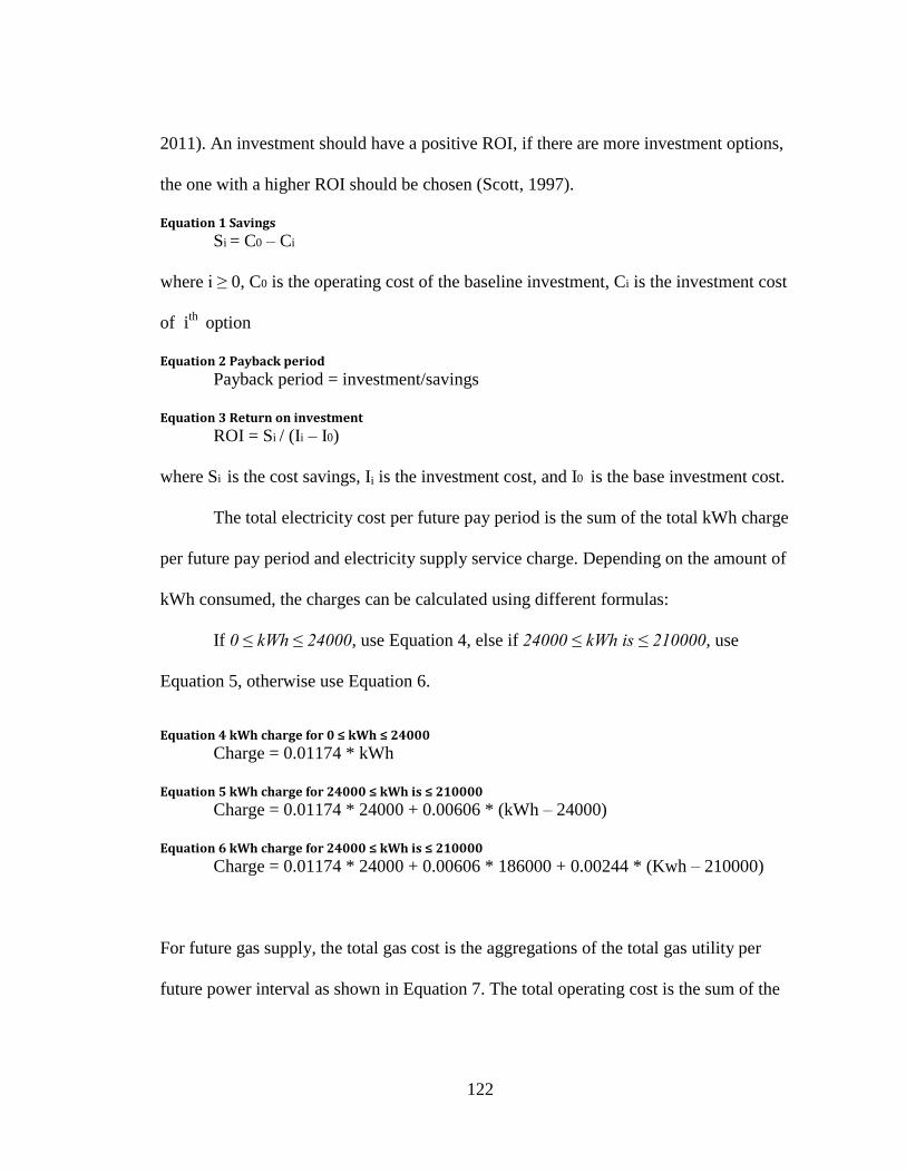
122

2011). An investment should have a positive ROI, if there are more investment options,

the one with a higher ROI should be chosen (Scott, 1997).

Equation 1 Savings

Si = C0 – Ci

where i ≥ 0, C0 is the operating cost of the baseline investment, Ci is the investment cost

of ith

option

Equation 2 Payback period

Payback period = investment/savings

Equation 3 Return on investment

ROI = Si / (Ii – I0)

where Si is the cost savings, Ii is the investment cost, and I0 is the base investment cost.

The total electricity cost per future pay period is the sum of the total kWh charge

per future pay period and electricity supply service charge. Depending on the amount of

kWh consumed, the charges can be calculated using different formulas:

If 0 ≤ kWh ≤ 24000, use Equation 4, else if 24000 ≤ kWh is ≤ 210000, use

Equation 5, otherwise use Equation 6.

Equation 4 kWh charge for 0 ≤ kWh ≤ 24000

Charge = 0.01174 * kWh

Equation 5 kWh charge for 24000 ≤ kWh is ≤ 210000

Charge = 0.01174 * 24000 + 0.00606 * (kWh – 24000)

Equation 6 kWh charge for 24000 ≤ kWh is ≤ 210000

Charge = 0.01174 * 24000 + 0.00606 * 186000 + 0.00244 * (Kwh – 210000)

For future gas supply, the total gas cost is the aggregations of the total gas utility per

future power interval as shown in Equation 7. The total operating cost is the sum of the

123

total electric cost and the total gas cost for all the future power intervals. Equation 8 is

used to calculate GHG amount.

Equation 7 total gas cost

Gas cost = (Σ (gas per interval/btuPerDth)) * gasPricePerDth

where btuPerDth is the amount of energy per dekatherm (1000000 BTU) and

gasPricePerDth is the gas charge per dekatherm ($6.5).

Equation 8 GHG emissions

MTCDEi = Gi * 0.053 MTCDE/Million-Btu + Pi * 0.513 MTCDE/Million-Wh

where, MTCDE is the Metric Tons of Carbon Dioxide Equivalent.

Equation 9 Cogen gas kWh conversion

cogenGasPerKwh = gasBTUPerGallon/kWhPerGallon/cogenGasToKwhEfficiency,

where cogenGasPerKwh is the amount of natural gas consumed by CoGen per

kWh, the amount of energy generated per gallon of gas gasBTUPerGallon is 114000

BTU, the energy generated per gallon of gas kwhPerGallon is 33.41 kWh, and the

efficiency of the CoGen plant to generate power from natural gas

cogenGasToKwhEfficiency is 0.33.

SPDA modeling: The SPDA models are developed to describe input data, KPIs, metrics,

optimization objective, and constraints according to the defined case scenario. Figure 47

through Figure 54 are modular SPDA model components. Figure 55 shows an analytical

query.

Figure 47 is the model for the “context” component timIntervals (), all global

variable are defined. Integer variables, nbPastPayPeriods and nbPayPeriods, float

variables, maxKwReductionPerPayPeriod and intervalSize, are represented using three

124

dots “…”. The three-dot separates the data model and SPDA model and enables the reuse

of SPDA models. AllPowerIntervals is declared as a set of strings for powerInterval.

powerInterval is a tuple consisting of seven integer attributes, “pInterval, payPeriod,

year, month, day, hour, and weekDay.” PastPowerIntervals is represented using a

negative number or 0. FuturePowerIntervals is a positive number that is larger than one.

pInterval is an hourly demand and payPeriod is a monthly demand.

context timeIntervals() {

int nbPayPeriods = ...;

int nbPastPayPeriods = ...;

float maxKwReductionPerPayPeriod = ...;

range FuturePayPeriods = 1 .. nbPayPeriods;

float intervalSize = ...;

tuple powerInterval {

int pInterval;

int payPeriod;

int year;

int month;

int day;

int hour;

int weekDay;

}

{ powerInterval} AllPowerIntervals = ...;

125

{ powerInterval} PastPowerIntervals =

{i | i in AllPowerIntervals : i.pInterval <= 0 };

{ powerInterval} FuturePowerIntervals =

{i | i in AllPowerIntervals : i.pInterval >= 1 };

}

Figure 47 Context model of facility heating/cooling and power case study

Figure 48 shows the model of the “flow” component flowSequence (Id). Id can be

replaced by an actual parameter in an include statement. The context model is included.

A one-dimensional array Id.amt is a positive float array, in which all elements are

positive float. Id.amt is indexed by a finite set of tuples. The elements of the array are the

amount of the flows at the power interval.

flow flowSequence (Id) {


include context timeIntervals();

float+ Id.amt[AllPowerIntervals];

}

Figure 48 Flow model of facility heating/cooling and power case study

Figure 49 shows the model of the “flow aggregator” component flowAggr. The context

model is included. Id.flowType is declared as a string flowSequence. Id.inputFlows and

126

Id.outputFlows are declared as a set of string and will be instantiated separately. Id.flows,

the union of Id.inputFlows and Id.outputFlows, are also a set of strings. Flow models for

all the flows in Id.flows are included. A constraint is that for each power interval. The

total amount of the inputFlows equals the total amount of the outputFlows.

flow aggregator flowAggr(Id) {


string Id.flowType = "flowSequence";




for (flow in Id.flows) include flow flowSequence(flow);

forall (i in AllPowerIntervals)

sum (flow in Id.inputFlows) flow.amt[i] ==

sum (flow in Id.outputFlows) flow.amt[i];

}

Figure 49 Flow aggregator model of facility heating/cooling and power case study

Figure 50 shows the electricity supply “process” model electricSupply (Id), that is an

atomic process. Id is provided when it is being included. The metrics are declared as a set

of two strings, cost and CO2. power is assigned as the name of every output flow (i.e.,

this process provides power to other processes). The flow model is included with a

127

parameter of the output flow. A positive float array variable,

utilityKw[AllPowerIntervals], an array of electricity supplied from the power utility

company over the AllPowerIntervals, is declared. The elements of arrays of

payPeriodSupplyDemand[FuturePayPeriods], an array of electricity demand over the

FuturePayPeriods; and demandReduction[FuturePowerIntervals], an array of extra

power supply that can be cut from the power inputs over the FuturePowerIntervals; are

also declared as positive float variables. historicUtilityKw[PastPowerIntervals] is an

array of past factory electric demand. payPeriodKwh[FuturePayPeriods] is the total

power consumption per future pay period. A piecewise function is used to compute kWh

cost using Equation 4, Equation 5, and Equation 6. The electricity supply service charge

generationDemandCharge[FuturePayPeriods] equals 8.124 times

payPeriodSupplyDemand[FuturePayPeriods]. The total electricity cost per future pay

period is the sum of the total kWh charge per future pay period and electricity supply

service charge.

process electricSupply(Id) {

include context timeIntervals ();

{string} Id.inputFlows = {};

string Id.powerFromUtility = …;

{string} Id.outputFlows = {Id.powerFromUtility};

string outputPowerFlow.name = "power";

include flow flowSequence(Id.powerFromUtility);

128

{string} Id.metrics = {"cost","CO2"};

for (flow in Id.outputFlows) {flow.name = "power";

include flow flowSequence(flow);}

float+ Id.utilityKw[AllPowerIntervals];

float+ Id.payPeriodSupplyDemand[FuturePayPeriods];

float Id.historicUtilityKw[i in PastPowerIntervals] = …;

float+ Id.demandReduction[FuturePowerIntervals];

float Id.payPeriodKwh[p in FuturePayPeriods] =

Sum(i in AllPowerIntervals : i.payPeriod == p) utilityKw[i];

pwlFunction Id.kwhCost =

piecewise {0.01174-> 24000;0.00606 -> 210000; 0.00244};

float Id.payPeriodKwhCharge[p in FuturePayPeriods] =

kwhCost (payPeriodKwh[p]);

float Id.generationDemandCharge[p in FuturePayPeriods] =

8.124 * payPeriodSupplyDemand[p];

float Id.cost = sum (p in FuturePayPeriods)

(payPeriodKwhCharge[p] + generationDemandCharge[p]);

float+ Id.outputPowerFlow.amt[i in AllPowerIntervals] =

Id.utilityKw[i];

}

Figure 50 Electricity supply process model of facility heating/cooling and power case study

129

Figure 51 shows the gas supply “process” model, gasSupply (Id), which is another atomic

process. The same metrics are declared as a set of two strings cost and CO2. gas is

assigned for every output flow as their names (i.e., the gas supply process provides gas to

other processes). The flow model is included with a parameter of the output flow. Then, a

positive float array variable, utilityGas[FuturePowerIntervals], an array of gas supply

from the gas utility company over the FuturePowerIntervals, is declared. The total gas

cost of all the FuturePowerIntervals is computed using Equation 7.

process gasSupply(Id) {


{string} Id.inputFlows = {};

string Id.gasFromUtility = …;

{string} Id.outputFlows = {Id.gasFromUtility};

string outputGasFlow.name = "gas";

include flow flowSequence (Id.gasFromUtility);

{string} Id.metrics = {"cost","CO2"};

float Id.gasPricePerDth = 6.5;

float Id.btuPerDth = 1000000.0;

float+ Id.utilityGas[FuturePowerIntervals];

float+ Id.cost = (sum (i in FuturePowerIntervals)

(Id.utilityGas[i]/Id.btuPerDth)) * Id.gasPricePerDth;

float outputGasFlow.amt[i in FuturePowerIntervals] = Id.utilityGas[i];

}

130

Figure 51 Gas process model of facility heating/cooling and power case study

Figure 52 shows the Current Heat and Cool Plant “process” model,

currentHeatCoolPlant (Id), which is another atomic process. The CHCP system needs

gas and electric power as the resources to generate heating and cooling for the factory.

The input string set includes strings of gasToCHCP and powerToCHCO. The output

string set includes heatFromCHCP and coolFromCHCP. allFlow is the union of

inputFlow and outflow. For every flow in allFlow, the flow model is included. Variables

of positive float arrays, gasIntoCHCP[FuturePowerIntervals],

kwIntoCHCP[FuturePowerIntervals], heatOutCHCP[FuturePowerIntervals], and

coolOutCHCP[FuturePowerIntervals], are declared. The constraints are added.

process currentHeatCoolPlant(Id) {


string Id.gasToCHCP = …;

string Id.powerToCHCP = …;

string Id.heatFromCHCP = …;

string Id.coolFromCHCP = …;

{string} Id.inputFlows = {Id.gasToCHCP, Id.powerToCHCP};

{string} Id.outputFlows = {Id.heatFromCHCP, Id.coolFromCHCP};

{string} Id.allFlows = Id.inputFlows union Id.outputFlows;

string Id.gasToCHCP.name = "gas";

131

string Id.powerToCHCP.name = "power";

string Id.heatFromCHCP.name = "heat";

string Id.coolFromCHCP.name = "cool";

for (f in Id.allFlows) include flow flowSequence(f);

float Id.gasPerHeatUnit = (1 / 0.78); //GasBTU/heatBTU

float Id.kwhPerCoolUnit = (1 / 0.94); //ton/kWH

float Id.chcpMaxHeatPerHr = 120000000.0; //Total existing capacity

Btu/hr

float Id.chcpMaxCoolPerHr = 12500; //Total existing capacity Ton/hr

float+ Id.gasIntoCHCP[FuturePowerIntervals];

float+ Id.kwIntoCHCP[FuturePowerIntervals];

float+ Id.heatOutCHCP[FuturePowerIntervals];

float+ Id.coolOutCHCP[FuturePowerIntervals];

forall (i in FuturePowerIntervals){

Id.heatOutCHCP[i] * Id.gasPerHeatUnit <= Id.gasIntoCHCP[i];

Id.coolOutCHCP[i] * Id.kwhPerCoolUnit <= Id.kwIntoCHCP[i] *

intervalSize;

Id.heatOutCHCP[i] <= Id.chcpMaxHeatPerHr * intervalSize;

Id.coolOutCHCP[i] <= Id.chcpMaxCoolPerHr * intervalSize;

}

float gasToCHCP.amt[i in FuturePowerIntervals] = Id.gasIntoCHCP[i];

float powerToCHCP.amt[i in FuturePowerIntervals] = Id.kwIntoCHCP[i];

float heatFromCHCP.amt[i in FuturePowerIntervals] = Id.heatOutCHCP[i];

float coolFromCHCP.amt[i in FuturePowerIntervals]= Id.coolOutCHCP[i];

132

}

Figure 52 Current heat and cooling process model of facility heating/cooling and power case study

Figure 53 shows the Co-generation “process” model, cogen (Id), which is also an atomic

process. The CoGen plant only needs gas to generate power, heat, and cooling for the

factory. The input string set is gasToCogen. The output string set includes

powerFromCogen, heatFromCogen, and coolFromCogen. allFlow is the union of

inputFlow and outflow. For every flow in allFlow, the flow model is included. Constants

are assigned. The amount of natural gas consumed per kWh is computed using Equation

9. Finally, the variables are connected to flows.

process cogen (Id) {


string Id.gasToCogen = …;

string Id.powerFromCogen = …;

string Id.heatFromCogen = …;

string Id.coolFromCogen = …;

{string} Id.inputFlows = {Id.gasToCogen};

{string} Id.outputFlows =

{Id.powerFromCogen,Id.heatFromCogen,Id.coolFromCogen};

{string} Id.allFlows = Id.inputFlows union Id.outputFlows;

string Id.gasToCogen.name = "gas";

133

string Id.powerFromCogen.name = "power";

string Id.heatFromCogen.name = "heat";

string Id.coolFromCogen.name = "cool";

for (f in Id.allFlows) include flow flowSequence(f);

float Id.cogenMaxHeatPerHr = 40000000.0; //Btu/hr

float Id.cogenMaxCoolPerHr = 2400.0; //ton/hr

float Id.cogenMaxKw = 7200.0; //kW

float Id.cogenGasToKwhEfficiency = 0.33;

float Id.gasBTUPerGallon = 114000.0;

float Id.kWhPerGallon = 33.41;

float Id.cogenGasPerKwh = Id.gasBTUPerGallon / Id.kWhPerGallon /

Id.cogenGasToKwhEfficiency; //BTU/kWh

float Id.cogenHeatPerKwh = 10300.0; //Btu/kWh = Net Heat Rate

float Id.cogenHeatToCoolRatio = Id.cogenMaxCoolPerHr /

Id.cogenMaxHeatPerHr;

float+ Id.gasIntoCogen[FuturePowerIntervals];

float+ Id.heatOutCogen[FuturePowerIntervals];

float+ Id.coolOutCogen[FuturePowerIntervals];

float+ Id.kwOutCogen[FuturePowerIntervals];


Id.kwOutCogen[i] * intervalSize * Id.cogenGasPerKwh <=

Id.gasIntoCogen[i];

Id.kwOutCogen[i] * intervalSize <= Id.cogenMaxKw;

Id.heatOutCogen[i] <= Id.cogenHeatPerKwh * Id.kwOutCogen[i]

134

* intervalSize;

Id.heatOutCogen[i] <= Id.cogenMaxHeatPerHr * intervalSize *

(Id.kwOutCogen[i]/Id.cogenMaxKw);

Id.coolOutCogen[i] <= (Id.cogenMaxHeatPerHr * intervalSize

* (Id.kwOutCogen[i]/Id.cogenMaxKw)- Id.heatOutCogen[i]) *

Id.cogenHeatToCoolRatio;

Id.coolOutCogen[i] <= Id.cogenMaxCoolPerHr * intervalSize;

// connect vars to flows

float gasToCogen.amt[i in FuturePowerIntervals] = Id.gasIntoCogen[i];

float powerFromCogen.amt[i in FuturePowerIntervals] = Id.kwOutCogen[i];

float heatFromCogen.amt[i in FuturePowerIntervals] =

Id.heatOutCogen[i];

float coolFromCogen.amt[i in FuturePowerIntervals] =

Id.coolOutCogen[i];

}

Figure 53 Co-gen process model of facility heating/cooling and power case study

Figure 54 is the facility heating, cooling, and power “process” model,

facilityHeatCoolPower (Id), which is a composite process. A one-dimensional float array

of historicDemandKw for past power intervals and power, heat, and cooling demands for

future power intervals are all assigned as three dots “…”. All the sub-processes, including

electricity and gas supplies, CHCP, and Cogen, are included. The next step is to construct

aggregators. For all sub-processes, flow names include gas, power, heat, and cool. A

135

string set, flowsFromSubProcesses, includes all output flows from all the sub-processes,

while another string set, flowsToSubProcesses, includes all input flows from all the sub-

processes. Flow models with parameters totalPower, totalHeat, and totalCool are

included. The input flows and output flows for every aggregator are defined. Constraints

regarding the supplies and demands are added. For example, the total generated power,

heat, and cool must be more than or equal to the demands for power, heat, and cool. Total

cost, the sum of power cost and gas cost, is defined.

process facilityHeatCoolPower () {

include context timeIntervals ();

// historical demand

float historicDemandKw[PastPowerIntervals] = …;

float demandKw[FuturePowerIntervals] = ...;

float demandHeat[FuturePowerIntervals] = ...;

float demandCool[FuturePowerIntervals] = ...;

{string} inputFlows = {};

{string} outputFlows = {};

{string} subProcesses = {"Dominion","WashGas","chcp","cogen"};

// sub processes

string Dominion.powerFromUtility = "powerFromUtility";

include process powerSupply("Dominion");

string WashGas.gasFromUtility = "gasFromUtility";

include process gasSupply("WashGas");

136

string chcp.gasToCHCP = "gasToCHCP";

string chcp.powerToCHCP = "powerToCHCP";

string chcp.heatFromCHCP = "heatFromCHCP";

string chcp.coolFromCHCP = "coolFromCHCP";

include process currentCoolHeatPlant("chcp");

string cogen.gasToCogen = "gasToCogen";

string cogen.powerFromCogen = "powerFromCogen";

string cogen.heatFromCogen = "heatFromCogen";

string cogen.coolFromCogen = "coolFromCogen";

include process cogen("cogen");

// aggregators construction

{string} flowNames = {"gas","power","heat","cool"};

{string} flowsFromSubProcesses = { f | s in subProcesses,

f in s.outputFlows};

{string} flowsToSubProcesses = { f | s in subProcesses,

f in s.inputFlows};

string totalPower.name = "power";

include flow flowSequence("totalPower");

string totalHeat.name = "heat";

include flow flowSequence("totalHeat");

string totalCool.name = "cool";

include flow flowSequence("totalCool");

{string} flowsIntoAggrs = flowsFromSubProcesses

{string} flowsFromAggrs = flowsToSubProcesses union

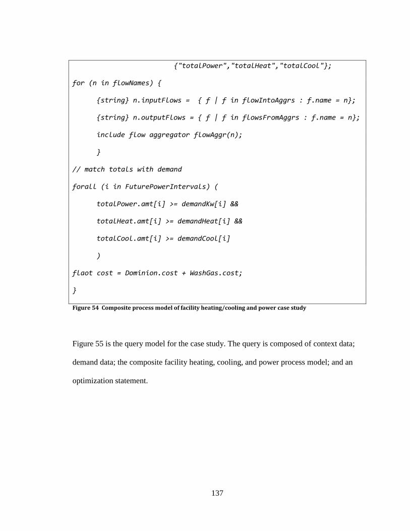
137

{"totalPower","totalHeat","totalCool"};

for (n in flowNames) {

{string} n.inputFlows = { f | f in flowIntoAggrs : f.name = n};

{string} n.outputFlows = { f | f in flowsFromAggrs : f.name = n};

include flow aggregator flowAggr(n);

}

// match totals with demand

forall (i in FuturePowerIntervals) (

totalPower.amt[i] >= demandKw[i] &&

totalHeat.amt[i] >= demandHeat[i] &&

totalCool.amt[i] >= demandCool[i]

)

flaot cost = Dominion.cost + WashGas.cost;

}

Figure 54 Composite process model of facility heating/cooling and power case study

Figure 55 is the query model for the case study. The query is composed of context data;

demand data; the composite facility heating, cooling, and power process model; and an

optimization statement.

138

include contextData ();

include demandData ();

include process facilityHeatCoolPower ();

minimize cost

Figure 55 Query of facility heating/cooling and power case study

Optimization solutions and recommendation: The SPDA query is translated to an OPL

model and solved by the IBM ILOG CPLEX. The following four proposed investment

options have been evaluated over the next 10 years (Brodsky, Ngan, Egge, & Backus,

2012).

(1) The expansion of the existing CHCP only,

(2) The addition of a CoGen plant to the existing CHCP,

(3) The half capacity of the Option (1) with the half planned capacity of the CoGen plant,

and

(4) The full capacity of the Option (1) with the full planned capacity of the CoGen plant.

The OPL program of this case study is listed in Appendix B. Table 5 and Table 6,

adopted from (Brodsky, Ngan, Egge, & Backus, 2012), are the optimization results.

Different evaluation parameters for ROI and GHG are listed for determining the best

investment option. Based on the parameter analysis, the Option (1) should be chosen

(Brodsky, Ngan, Egge, & Backus, 2012) because of:

The GHG emissions are the lowest.

139

Even though the ROI of the Option (2) is marginally better than that of the Option

(1), the GHG emissions of the Option (2) is the highest among all four options.

The investment amount of the Option (2) is not feasible.

Table 5 Evaluation parameters of ROI

Investment

Option

Investment

Cost ($M)

Annual

Mainte

nance

Cost ($)

Annualized

Replacement

Cost ($M)

Annualized

Equipment

Cost ($M)

Annualized

Average

Operational

Cost ($M)

Annualized

Saving

over the

Expanded

CHCP

($M)

ROI

(%)

1 Expanded

CHCP

$34.293 $343,20

0

$3.429 $3.772 $6.244 $0.000 0.00

0 %

1 CoGen

Plant + 1

Current

CHCP

$65.328 $655,60

0

$3.850 $4.506 $5.494 $0.016 0.05

2 %

½ CoGen

Plant + ½

Expanded

CHCP

$46.995 $499,40

0

$4.699 $5.199 $5.557 -$0.740 -

5.82

7 %

1 CoGen

Plant + 1

Expanded

CHCP

$99.621 $998,80

0

$7.279 $8.278 $5.492 -$3.754 -

5.74

7 %

Table 6 Evaluation parameters of GHG emissions

Investment Option Investment Cost

($M)

Average Annual

Gas Consumption

(MBTU)

Average Annual

Electric Power

Consumption

(MWh)

GHG Emission

(MTCDE)

1 Expanded CHCP $34.293 510,500.00 141,433.33 99611.799

1 CoGen Plant + 1

Current CHCP

$65.328 523,622.22 141,333.33 100255.977

½ CoGen Plant +

½ Expanded

CHCP

$46.995 520,888.89 141,344.44 100116.811

1 CoGen Plant + 1

Expanded CHCP

$99.621 523,600.00 141,333.33 100254.799

140

5.3 Case Study 2 - Operational control for sustainable machining The second case study, sustainable machining, is described in this section. Machining is

one of the major unit manufacturing processes. It involves a number of sustainability

performance indicators that can be potentially improved. The sustainability performance

indicators for machining processes include tool life, coolant and lubricant usage, solid

waste, and energy consumption as discussed in (Bengtsson, Michaloski, Proctor, Shao, &

Venkatesh, 2010).

This case study assists decision-making for a machining center purchase by

determining optimal cutting conditions (spindle and cutting speed) that lead to the most

energy efficient and environmentally friendly machining. Desmira, Narita, and Fujimoto

(2009) indicate “The spindle speed of conventional milling is relatively slow and it

results in a longer machining time and causes an unnecessary excess of carbon dioxide

emissions.” The energy consumption can be lowered if the spindle speed is increased, as

this reduces the overall machining time. However, finding the optimal speed for

machining operation can be very complex. The environmental impact due to the

consumption of other machine parts and tooling need to be taken into account. Eventually

the disposal of solid waste, and used tools and liquids also causes an effect on the

environment.

Problem formulation: This case scenario is adopted from (Desmira, Narita, & Fujimoto,

2009), a machining center that uses a 10 mm diameter carbide square coating cutting tool.

The flute number is 6 and number of teeth is 2. The axial depth is 0.1 mm, the radial

depth is 10 mm, and cutting length is 60 m. The objective of the study is to determine the

141

appropriate cutting conditions that minimize the total CO2 emissions due to the

machining process. The case study has been implemented in (Shao G. , Kibira, Brodsky,

& Egge, 2011) using DGQL. Figure 56 illustrates the inputs and outputs of SPDA

modeling. The following activities are involved:

1. Develop metrics for assessing the performance of a machining process. All factors

including electricity consumption, tool usage, lubricant, coolant, and material chips

are converted to equivalent CO2 emissions and aggregated. The optimal cutting

conditions are obtained for the lowest total emissions.

2. Design and deploy a data collection methodology. Data for machine, tool, coolant,

lubricant, and material are extracted from LCI database, production database, and

machine tool specifications.

3. Develop SPDA models and query, translate the models to OPL, and solve the OPL

model with the IBM ILOG CPLEX.

Figure 57 illustrates the input and output flows of a machining process. Figure 58 shows

an example of a real machining center and its virtual model, which is adopted from

(Shao, Lee, & McLean, 2003).

142

- Energy

- CO2 Emission

- Cutting speed

- Spindle speed

- Cost

LCI

NC program

Machine

specifications

Knowledge Base Storage

Product

design

Sustainable Process

Description and Analytics

(SPDA) Formalism

Kn

ow

led

ge

Decis

ion

Reco

mm

en

dati

on

Constraints

Objective

Designation

Energy

consumption

Model Input Data

Metrics

External Mathematical

Solver (IBM ILOG CPLEX)

Figure 56 Sustainable machining SPDA modeling diagram

Sustainable machining

Energy

Solid waste

LubricantCoolant

CO2 EmissionLiquid waste

Finished

productWorkpiece

Cutting tool NC

Figure 57 Machining process input and output flows diagram

143

Figure 58 An example of a real machining center and its virtual model (Shao & Lee, 2007)

Sustainable machining data and knowledge collection: Since LCA is performed, the

functional unit and the products of LCA study need to be determined. The ISO 14040

standard provides a framework for LCA. The functional unit is a measure of the function

of the studied system and provides a reference to which the inputs and outputs can be

related (ISO 14040, 2006). In this case study, the LCA functional unit is defined as - for

one specific part, a given NC program, with given material and the weight of the stock.

The potential environmental impacts throughout a product’s lifecycle (i.e., cradle-to-

grave) from raw material acquisition through production, use, and disposal are

considered. The LCA products are machined part, cutting tool, coolant, and lubricant oil.

The LCI data used and the formulas (Equation 10 through Equation 16) used are adopted

from (Narita & Fujimoto, 2009).

Total environmental impact (Pe): The total environmental impact is calculated

from machining electricity consumption, coolant and lubricant oil usage, cutting tool

status, and metal chip quantity as follows:

144

Equation 10 Total environmental impact

Pe = Ee + Ce+LOe+ )(1

N

iieT +Che

where

Pe: Environmental impact of machining operation (kg-GAS)

Ee: Environmental impact of machine tool electricity consumption (kg- GAS)

Ce: Environmental impact of coolant (kg- GAS)

LOe: Environmental impact of lubricant oil (kg- GAS)

Te: Environmental impact of cutting tools (kg- GAS)

Che: Environmental impact of metal chips (kg- GAS)

N: Number of tools used in NC programs

GAS corresponds to equivalent emission factors for each impact category.

Calculation algorithms for the above factors, Ee, Ce, LOe, Te, and Che, are presented in

the following subsections.

Machine tool electricity consumption (Ee):

Equation 11 Total electricity consumption of machine tool

Ee= k× (SME+SPE+SCE+CME+CPE+ TCE1+ TCE2+ATCE+MGE+SBE)

where

k: CO2 emission intensity of electricity (kg-GAS/kWh)

SME: Servomotor electricity consumption (kWh)

SPE: Spindle motor electricity consumption (kWh)

SCE: Spindle cooling system electricity consumption (kWh)

CME: Compressor electricity consumption (kWh)

CPE: Coolant pump electricity consumption (kWh)

145

TCE1: Chip conveyor electricity consumption (kWh)

TCE2: Machine tool chip conveyor electricity consumption (kWh)

ATCE: Auto tool changer electricity consumption (kWh)

MGE: Tool magazine motor electricity consumption (kWh)

SBE: Machine tool standby energy (kWh)

Coolant (Ce): Two types of cutting fluid exist, so there are two parts in Equation

12 for evaluating Ce. In the case of water-miscible cutting fluid, coolant is generally used

to enhance machining performance and circulated in machine tools by coolant pumps.

During the usage period, some coolants are consumed by adhering to metal chips, and

need to be supplied to compensate the loss. The reduction in dilution fluid (water) due to

vapor also need to be considered in estimating total coolant.

Equation 12 The environmental impact of coolant

Ce = CUT/CL× {(CPe+CDe) × (CC+AC) +WAe× (WAQ+AWAQ)}

where

CUT: Coolant usage time in NC programs (s)

CL: Mean coolant update interval (s)

CPe: Environmental impact of cutting fluid production (kg-GAS/L)

CDe: Environmental impact of cutting fluid disposal (kg-GAS/L)

CC: Initial coolant quantity (L)

AC: Additional supplementary coolant until coolant is replaced (L)

WAe: Environmental impact of water distribution (kg-GAS/L)

WAQ: Initial water quantity (L)

AWAQ: Additional supplementary water until coolant is replaced (L)

146

Equation 13 The environmental impact of coolant with water-insoluble cutting fluid

Ce=CUT/3600×CS/1000× (CPe+CDe)

where

CS: Cutting fluid discharge rate (cc/h)

Lubricant oil (LOe): Lubricant oil is used for spindles and slideways. The

amounts of oil-air lubricant supplied by a pump to spindles within a specific interval are

considered.

Equation 14 The environmental impact of lubricant oil

LOe= SRT/ SI ×SV× (SPe+SDe) + LUT/LI×LV ×(LPe+LDe)

where

SRT: NC program spindle runtime (s)

SV: Spindle lubricant oil discharge rate (L)

SI: Mean interval between discharges (s)

SPe: Environmental impact of spindle lubricant oil production (kg-GAS/L)

SDe: Environmental impact of spindle lubricant oil disposal (kg-GAS/L)

LUT: NC program slideway runtime (s)

LI: Mean interval between supplies (s)

LV: Lubricant oil quantity supplied to slideway (L)

LPe: Environmental impact of slideway lubricant oil production (kg-GAS/L)

LDe: Environmental impact of slideway lubricant oil disposal (kg-GAS/L)

The same equations can be used to calculate the environmental impact for grease.

147

Cutting tool (Te): Cutting tools’ environmental impact are calculated based on

tool life and machining time of machining processes. Cutting tools, especially for solid

end mills, are renewed by regrinding.

Equation 15 The environmental impact of cutting tool

Te = MT/1

1

RN

j

TLj × ((TPe+TDe) ×TW+RN×RGe)

where

MT: Machining time (s)

TL: Tool life (s)

TPe: Environmental impact of cutting tool production (kg-CO2/kg)

TDe: Environmental impact of cutting tool disposal (kg-GAS/kg)

TW: Tool weight (kg)

RN: Total number of recoveries

RGe: Environmental impact due to recovery (kg-GAS)

Metal chips (CHe):

Equation 16 The environmental impact of metal chips

CHe = (WPV-PV) ×MD ×WDe

where

CHe: Environmental impact of metal chips in carbon dioxide equivalents (kg- CO2)

WPV: Stock volume (cm³)

PV: Product volume (cm³)

MD: Stock material density (kg/ cm³)

WDe: Environmental impact of metal chip processing (kg- CO2/kg)

148

Conceptual modeling: The dependency relationships among the indicators and attributes

are needed for SPDA modeling. Brodsky and Wang (2008) describe that the dependence

graph can capture the relationship among parameters. A dependency graph is composed

of a set of connectors that have input and output attributes. An associated transformer can

represent partial knowledge on how outputs are computed from the inputs and relate the

values of these parameters. Based on the formulas discussed above, a dependence graph

is developed to capture parameters for the machining case. Figure 59 shows a partial

dependence graph for the total emissions. Circles represent parameters, e.g.,

cuttingSpeed, toolLife, and totalEmission. Boxes represent dependence connectors, e.g.,

Emission and Waste. Single-line boxes represent deterministic connectors. For example,

the waste connector suggests that the value of its output metalChipEmission is

deterministically dependent on its input parameters stockVolume, productVolume, and

materialDensity, and the environmental impact from production and disposal. Double-

line boxes represent stochastic connectors. For example, the dependence connector

CSpeed, as shown in Figure 59, suggests that its output machiningTime, is dependent on

the value of its input parameter spindleSpeed, which is a decision variable.

149

C

totalEmissionE

Emission

electricityConsumptionEmission

coolantEmission

lubricantEmission

cuttingToolsEmission

metalChipsEmission

CT

L

machiningTime

CSpeed

spindleSpeed

toolLife

stockVolume

materialDensity

Waste fromProcessing

productVolume

numberofRecoveries

toolWeight

materialDensity

fromRepair

fromProduction

fromDisposal

Key:

E: Electricity Consumption

C: Coolant

L: Lubricant

CT: Cutting Tool

CSpeed: Cutting Speed

Figure 59 Dependency graph model for cutting speed vs. CO2 emission

In Figure 59, the output value of each box has two possibilities: decrease or increase.

Electricity consumption, coolant quantity, and lubricant oil quantity are determined by

the machining time. These factors are decreased as machining time is decreased. On the

other hand, the environmental impact of cutting tool is managed from the tool life. Tool

life is determined by tool wear, which is a more complex research area. The details of

how tool wear affects environmental impact are out of the scope of this dissertation.

Data acquisition: As indicated in Figure 59, the total CO2 emissions depend on the only

decision variable, spindleSpeed. machiningTime and toolLife are affected by the spindle

speed. The rest of the parameters are constants, they are mainly LCI data and machine

specification data. To simplify the problem, all the emissions (Equation 17) except from

150

the cutting tool (Equation 18) are combined. Thus, only two components need to be

modeled (Equation 19):

Equation 17 CO2 emissions due to the cutting process

Ep = electricityConsumptionEmission + coolantEmission + lubricantEmission

Equation 18 CO2 emissions resulting from the cutting tool

Ec = cuttingToolEmission

These two components make up the totalEmission, i.e.,

Equation 19 Total emission

ET = Ep + Ec

In general, the higher the cutting speed is, the shorter the machining time is

needed and the lower the amount of the CO2 is emitted (Ep). On the other hand, the tool

wear and tool life are also dependent of cutting time, as the spindle speed increases up to

a point, the emission Ec from the cutting tool starts to go up. Thus, overall CO2 emission

gradually increases after the cutting speed reaches at a certain point. The Taylor Equation

for Tool Life provides a good approximation ( (Kalpakjian & Schmidt, 2002). The

equation is represented in two forms, shown in Equation 20 and Equation 21.

Equation 20 Taylor tool life equation

Or in the form of:

Equation 21 Generic version of Taylor tool life equation

where

is cutting speed,

T is tool life,

151

D is depth of cut, S is feed rate,

x and y are determined experimentally, and

n and C are parameters, which depend on S, D, workpiece and tool material, they can be

found by experimentation or published data.

However, using Taylor Equation introduces more complexity. The optimization

solver solves linear optimization problems. The empirical data derived from (Desmira,

Narita, & Fujimoto, 2009), as shown in Figure 60, Figure 61, and Table 7, are used to

indicate the relationship between spindle speed and emissions, and spindle speed and

cutting time or tool life respectively. During the translation from SPDA model to OPL

model, the tool emission module is modeled with a piecewise linear function to represent

the emission due to cutting tool. In this case study, the decision variable is machining

time.

Figure 60 Experimental emission data from both process and cutting tool

0

200

400

600

800

1000

1200

700 1600 2500 3500 5000 6400 6800

Other processes

Cutting tool

Total

Spindle Speed

Emissions

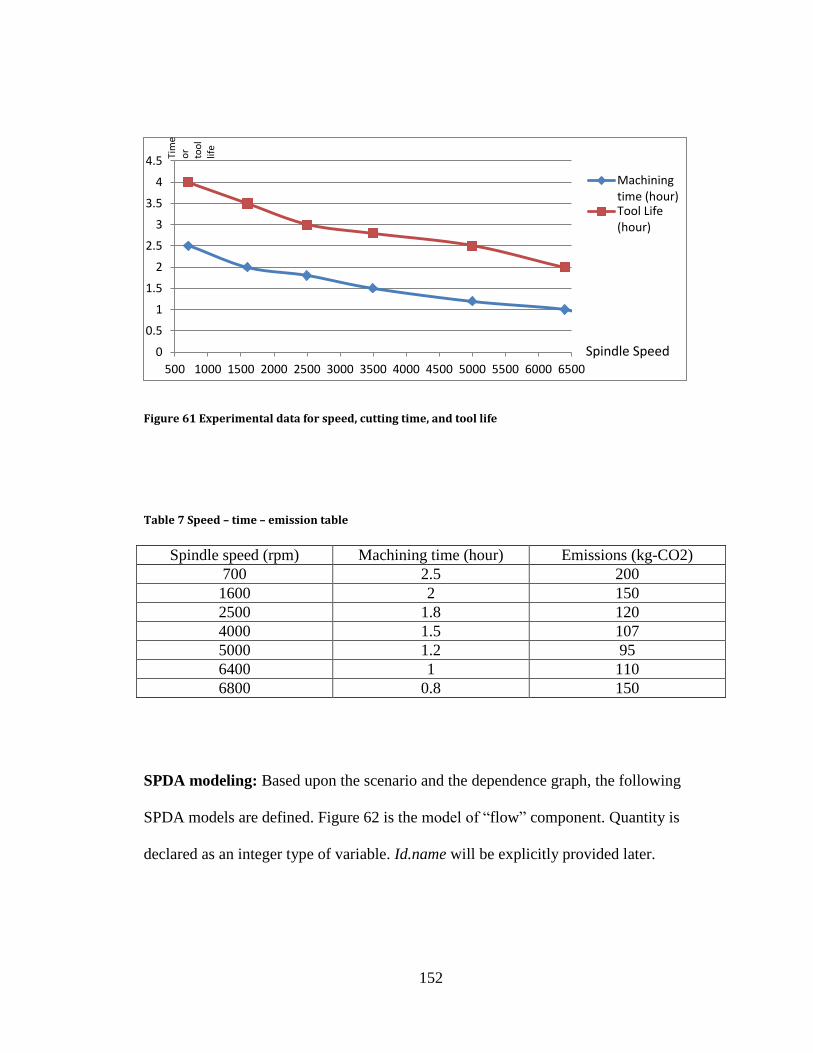
152

Figure 61 Experimental data for speed, cutting time, and tool life

Table 7 Speed – time – emission table

Spindle speed (rpm) Machining time (hour) Emissions (kg-CO2)

700 2.5 200

1600 2 150

2500 1.8 120

4000 1.5 107

5000 1.2 95

6400 1 110

6800 0.8 150

SPDA modeling: Based upon the scenario and the dependence graph, the following

SPDA models are defined. Figure 62 is the model of “flow” component. Quantity is

declared as an integer type of variable. Id.name will be explicitly provided later.

0

0.5

1

1.5

2

2.5

3

3.5

4

4.5

500 1000 1500 2000 2500 3000 3500 4000 4500 5000 5500 6000 6500

Machiningtime (hour)Tool Life(hour)

Spindle Speed

Tim

e o

r

too

l lif

e

153

flow item (Id) {


int Id.quantity;

}

Figure 62 Flow model for the machining case

A computation model milling, as shown in Figure 63, is developed for the total

emissions, in which a variable, machining time Mt, is declared. The total emissions for

the machining process due to electricity consumption, coolant usage, lubricant usage,

cutting tool, and waste are computed and aggregated.

process milling (Id) {

float k = … ; // CO2 emission intensity of electricity (kg-

GAS/kWh)

{string} powerParameter = … ;

float powerParameter_value[powerParameter] = … ;

{string} lubriParameter = … ;

float lubriparameter_value[lubriParameter] = … ;

{string} coolantParameter = … ;

float coolantParameter_value[coolantParameter] = … ;

{string} toolParameter = … ;

float toolParameter_value[toolParameter] = … ;

int numRecov = … ;

154

float TL[1..numRecov] = …;

{string} tools = …;

{string} wasteParameter = … ;

float wasteParameter_value[wasteParameter] = … ;

float powerEmission = Mt * k * sum (p in powerParameter)

powerParameter_value[p];

float luricnatEmission = Mt/lubriparameter_value[SI]*

lubriparameter_value[SV]*(lubriparameter_value[SPe]+

lubriparameter_value[SDe])+ Mt/lubriparameter_value[LI]*

lubriparameter_value[LV]*(lubriparameter_value[LPe]+

lubriparameter_value[LDe]);

float coolantEmission = Mt/coolantParameter_value[cl]*

(( coolantParameter_value[CPe] +

coolantParameter_value[CDe]) *

(coolantParameter_value[CC] + coolantParameter_value[AC])

+ coolantParameter_value[WAe]*(coolantParameter_value[WAQ]

+ coolantParameter_value[AWAQ]));

for (t in tools) sum {

float toolEmission =

Mt/sum (j in 1..numRecov)TL[j] *((powerParameter_value[TPe] +

powerParameter_value[TDe])*powerParameter_value[TW] +numRecov*

powerParameter_value[RGe]);

155

}

float wasteEmission = (wasteParameter_value[WPV]-

wasteParameter_value[PV])* wasteParameter_value[MD]*

wasteParameter_value[WDe];

float machiningEmission = powerEmission + luricnatEmission +

coolantEmission + toolEmission + wasteEmission;

}

Figure 63 An atomic sustainable milling machining process model

A reusable machining process, machiningProcess (Id), is shown in Figure 64. It includes

the atomic computational model for milling machines. As a unit process on the factory

floor, this SPDA machining process is designed in a way that it can be included multiple

times in a machine shop modeling. Output flow of one machine may be the input flow of

other machines. Figure 65 is the data model for this case. Figure 66 is the analytical

query, which simply includes the data, the process model, and the optimization statement.

process machiningProcess (Id) {

string Id.inputWorkpiece = …;

string Id.outputFinishedProduct = …;

{string} Id.inputFlows= Id.inputWorkpiece;

{string} Id.outputFlows= Id.outputFinishedProduct;

include flow item (Id.inputWorkpiece);

include flow item (Id.outputFinishedProduct);

156

int Id.inputWorkpiece.quantity =

Id.outputFinishedProduct.quantity

include process milling (machine);

float Id.CO2 = machine.CO2 * Id. outputFinishedProduct.quantity;

float Id.energy = machine.energy *

Id. outputFinishedProduct.quantity;

}

Figure 64 Composite process model for milling process

data () {

float k = 10.0; // CO2 emission intensity of electricity

{string} powerParameter = {“sme”, “spe”, “sce”, “cme”, “cpe”,

“tce1”,“tce2”, “atce”, “mge”, “sbe”};

float powerParameter_value [powerParameter] = [“sme”: 0.1,

“spe”: 0.06, “sce”: 0.45, “cme”: 1, “cpe”: 0.25, “tce1”:

0.7,“tce2”: 0.6, “atce”: 0.08, “mge”: 0.087, “sbe”: 0.64];

{string} lubriParameter = {"SI", “SV”, “SPe”, “SDe”, “LI”, “LV”,

“LPe”,“LDe”};

float lubriparameter_value[lubriParameter] = ["SI": 480.0, “SV”:

0.03, “SPe”: 0.9776, “SDe”: 0.0029, “LI”: 2000, “LV”: 228,

“LPe”: 0.1,“LDe”: 0.001];

157

{string} coolantParameter = {"cl", “CPe”, “CDe”, “CC”, “AC”,

“WAe”, “WAQ”,“AWAQ”};

float coolantParameter_value [coolantParameter] = ["cl":

720*60*60, “CPe”: 0.25, “CDe”: 0.06, “CC”: 0.175, “AC”:

0.08225, “WAe”: 0.189, “WAQ”:0,“AWAQ”: 0];

{string} toolParameter = {“TPe”, “TDe”, “TW”, “RGe”};

float toolParameter_value [toolParameter] = [“TPe”:33.7478,

“TDe”: 0.01346, “TW”: 0.25, “RGe”: 0.0184];

int numRecov = 3;

float TL [1..numRecov] = [10000, 8000, 5000];

{string} tools = {"tool1","tool2"};

{string} wasteParameter = {"WPV", “PV”, “MD”, “WDe”};

float wasteParameter_value [wasteParameter] = ["WPV": 40, “PV”:

30, “MD”: 7.1, “WDe”: 30];

}

Figure 65 Data model of the sustainable machining case

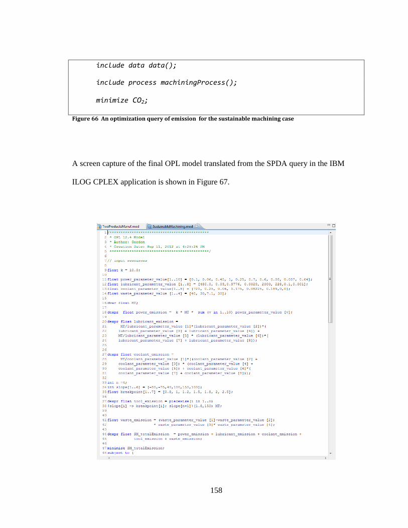
158

include data data();

include process machiningProcess();

minimize CO2;

Figure 66 An optimization query of emission for the sustainable machining case

A screen capture of the final OPL model translated from the SPDA query in the IBM

ILOG CPLEX application is shown in Figure 67.

159

Figure 67 OPL model screen capture for the sustainable machining case

Optimization solutions and recommendations: The sustainable machining case study

represents a simplified optimization problem. The OPL model translated from the SPDA

query is executed in the IBM ILOG CPLEX. Figure 68 shows an OPL execution solution

screen. The optimal machining time is 1 hour. According to the data in Table 7, the

optimal cutting speed is 6400 rpm.

Figure 68 Optimization results of machining time using IBM ILOG CPLEX

The cutting conditions such as the cutting speed and feed rate can be calculated based on

Equation 22 and Equation 23.

160

Equation 22 Tool cutting speed

Vc = 1000

** nd

where Vc is in meters/min, the diameter d is in mm, and n is in revolutions per minute.

Equation 23 Tool feed rate

Vf = fz*z*n =d

Vzf cz

*

*1000**

where Vf is in mm/min, fz is the feed per tooth, and z is the number of teeth. Where d, fz,

and z are all given in the beginning of this section.

The conclusion of this case study is that the cutting conditions for the lowest total

emissions are 6400 rpm for spindle speed, 201.06 m/min for cutting speed, and 1280

mm/min for feed rate. This leads to an investment recommendation for the high-speed

machining center. The optimization case study has shown that high-speed milling,

characterized by a spindle rotation speed that is five to ten times faster than conventional

milling (Shao G. , Kibira, Brodsky, & Egge, 2011), can be beneficial to SM.

161

6. CONCLUSION

The key contributions of this dissertation research include:

1. Developed a sustainable manufacturing-decision-guidance methodology that provides

step-by-step procedures for sustainability performance analysis and decision guidance

using the SPDA formalism for both operational and investment/planning decisions for

SM.

2. Developed the sustainable process description and analytics (SPDA) formalism for

SM knowledge representation, analysis, and optimization to support the sustainable

manufacturing-decision-guidance methodology. The formalism includes three major

parts.

(4) SPDA generic analytics language - provides unified syntax and semantics for

process modeling and support data querying, what-if analysis, and decision

optimization. The SPDA formalism enables modular, extensible, and reusable

models.

(5) SPDA process description and sustainability metrics - enable formal

representation of process structure, resource flow, data, control parameters,

objectives, and constraints; support sustainable metrics models; and are easy to

use by manufacturing and business users at a factory floor.

162

(6) A reduction procedure - enables the translation of SPDA queries into specialized

models such as optimization models to generate actionable recommendations for

SM improvement.

3. Developed categorizations of potential case studies for SM using SPDA and

performed one case study from each of the two categories to demonstrate the

developed formalism and proposed methodology:

(3) Investment/planning for energy efficient manufacturing: making a decision on

facility energy generation equipment investment with respect to optimal cost and

emissions.

(4) Operational for sustainable manufacturing: making a machining center purchase

decision based on optimal spindle speed that leads to minimal emissions.

The SPDA formalism allows manufacturing and business users effectively describe

sustainable process analytics knowledge. Compared to traditional optimization methods,

the SPDA makes what-if analysis and decision optimization for SM more intuitive and

user friendly and enables the creation of SPDA model components library for reuse.

This dissertation has done the first and critical step, but many interesting research

questions remain open. Future research may include (1) developing graphical

representation of SPDA using UML, BPMN, or SysML to model process structures; (2)

developing SPDA translators that automatically translate SPDA query to AMPL, OPL, or

other decision support tools such as DES; (3) designing graphical user interfaces to

enable drag-and-drop process modeling and push-button solutions; (4) enhancing SPDA

to represent manufacturing unit processes, manufacturing assembly processes, production

163

planning, and supply chain; (5) developing stochastic modeling to express SM metrics

that are dependent on random variables through a simulation-like model; (6) creating

common models for sustainability indicators and metrics based on the research results

from NIST SM program; (7) implementing more complex real world case studies to

identify new requirements for enhancing the SPDA formalism; and (8) standardizing the

SPDA formalism to enable more manufacturing industries to benefit from this research.

164

APPENDIX A – PROOF OF CLAIM 1 (CORRECTNESS OF SPDA

QUERY COMPUTATION ALGORITHM)

Claim 1: Algorithm SPDA query computation is CORRECT, i.e., it is:

1. Sound, i.e., for every well-formed analytical query (A, P),

All_Ans (A, P) ⊆ All_Sem (A, P)

2. Complete, i.e., for every well-formed analytical query (A, P),

All_Sem (A, P) ⊆ All_Ans (A, P)

The proof of the correctness of the SPDA query computation algorithms is as follows:

Soundness:

Assuming that (A’, P’) ∈ All_Ans (A, P), we need to prove that (A’, P’) ∈All_Sem (A, P).

The construction of the flat sequence S2 of Algorithm 1 (Steps 1 and 2) is exactly

as in the definition of Sem (A, P). In addition, Step 6 constructs (A’, P’) from sequence

S3, which is also exactly as defined in Sem (A, P). Therefore, the only remaining part is

to show that the flat analytical sequence S3 computed from S2 in Step 5 of Algorithm 1 is

indeed Sem (A, P), i.e., it is in All_Sem (A, P). Consider Algorithm 2, which computes

S3 from S2 = (s1, ..., sn, s(n+1)).

Case 1: if Algorithm 2 returns “INFEASIBLE,” then, the optimization problem O (in

Step 5 of Algorithm 2) is infeasible. Therefore, by construction of O and the

165

definition of alternative sequence semantics (see section 3.4), Sem (s1, ..., sn) = ∅

Therefore, the semantics of S2, Sem (S2), is INFEASIBLE.

Case 2: if Algorithm 2 returns “UNBOUNDED,” then, by construction of O and the

definition of explicit analytical sequence E in Sem (s1, ..., sn), E does not exist.

Therefore, Sem (S2) is UNBOUNDED by definition of optimization sequence

semantics.

Case 3: if Algorithm 2 returns a sequence (s1’, ..., sn’) that is constructed in Step 7 of

Algorithm 2, then, by construction of (s1’, ..., sn’) from the solution of

optimization problem O, (s1’, ..., sn’) ∈ Sem (s1, ..., sn), where Sem (s1, ..., sn) is

the alternative sequence semantics defined in Section 3.4.

Furthermore, E = (s1’, ..., sn’) satisfies the conditions in the definition of

optimization sequence semantics defined in Section 3.4.

In summary, we have (A’, P’) ∈ All_Ans (A, P) and (A’, P’) ∈ All_Sem (A, P), so

All_Ans (A, P) ⊆ All_Sem (A, P).

Completeness:

Assuming that (A’, P’) ∈ All_Sem (A, P), we need to prove that (A’, P’) ∈All_Ans (A, P).

The flat sequence S2 in the definition of Sem (A, P) is exactly as in the

construction of the flat sequence S2 of Algorithm 1 (Steps 1 and 2). In addition, the

constructed (A’, P’) from sequence S3 in the definition of Sem (A, P) is exactly as in the

construction of in Step 6 of Algorithm 1. Therefore, the only remaining part is to show

166

that S3 = Sem (S2), which is a flat analytical sequence, is indeed computed from S2= (s1,

..., sn, s(n+1)) in Step 5 of Algorithm 1. Consider S3, which is defined in Sem (A, P):

Case 1: if Sem (S2) is “INFEASIBLE,” then, by definition of Sem (S2), Sem (s1, ..., sn)

= ∅. Therefore, by construction of the optimization problem O (in Step 5 of

Algorithm 2), O is infeasible. Therefore, Algorithm 2 returns “INFEASIBLE.”

Case 2: if Sem (S2) is “UNBOUNDED,” then, by definition of Sem (S2), the explicit

analytical sequence E is the definition of Sem (S2) (see Section 3.4). Therefore,

by construction of the optimization problem O (in Step 5 of Algorithm 2), it must

be “UNBOUNDED,” and so Algorithm 2 must return “UNBOUNDED.”

Case 3: if there exists an explicit analytical sequence E that is Sem (S2), then, E must

satisfy the definition of Sem (S2) (see Section 3.4). Therefore, by construction of

the optimization problem O (in Step 5 of Algorithm 2), E must correspond to a

possible optimal solution of the problem O. Therefore, E ∈ All_Ans (A, P).

In summary, we have (A’, P’) ∈ All_Sem (A, P) and (A’, P’) ∈ All_Ans (A, P), so

All_Sem (A, P) ⊆ All_Ans (A, P).

167

APPENDIX B – OPL CODE FOR CASE STUDY OF

INVESTMENT/PLANNING FOR ENERGY EFFICIENT

MANUFACTURING

For the purpose of completeness, The OPL model for the case study of

investment/planning for energy efficient manufacturing is listed here. It was developed

by Brodsky and Ngan (2012). /*******************************************

* OPL 12.4 Cogeneration Plant Analysis *

* Author: Alex Brodsky and Chun-Kit Ngan *

* Creation Date: July 24, 2012 at 8:28PM *

* Updated Date: August 12, 2012 at 03:15PM*

*******************************************/

//General Input Data

int nbPayPeriods = ...;

int nbPastPayPeriods = ...;

float maxKwReductionPerPayPeriod = ...;

range FuturePayPeriods = 1 .. nbPayPeriods ;

float intervalSize = 1.0;

tuple powerInterval{

int pInterval;

int payPeriod;

int year;

168

int month;

int day;

int hour;

int weekDay;

}

{powerInterval} AllPowerIntervals = ...;

{powerInterval} PastPowerIntervals = {i | i in AllPowerIntervals :

i.pInterval <= 0};

{powerInterval} FuturePowerIntervals = {i | i in AllPowerIntervals :

i. pInterval >= 1};

//Demand Input Data

float demandKw[AllPowerIntervals] = ...;

float demandHeat[FuturePowerIntervals] = ...;

float demandCool[FuturePowerIntervals] = ...;

//Electric Cost

dvar float+ utilityKw[AllPowerIntervals];

dvar float+ payPeriodSupplyDemand[FuturePayPeriods];

float historicUtilityKw[i in PastPowerIntervals] = demandKw[i];

dvar float+ demandReduction[FuturePowerIntervals];

dexpr float payPeriodKwh[p in FuturePayPeriods] =

169

sum(i in AllPowerIntervals : i.payPeriod == p)

utilityKw[i];

pwlFunction kwhCost = piecewise {0.01174-> 24000; 0.00606 -> 210000;

0.00244};

dexpr float payPeriodKwhCharge[p in FuturePayPeriods] =

kwhCost(payPeriodKwh[p]);

dexpr float generationDemandCharge[p in FuturePayPeriods] = 8.124 *

payPeriodSupplyDemand[p];

dexpr float electricCost = sum(p in FuturePayPeriods)

(payPeriodKwhCharge[p] +

generationDemandCharge[p]);

//Gas Cost

float gasPricePerDth = 6.5;

float btuPerDth = 1000000.0;

dvar float+ utilityGas[FuturePowerIntervals];

dexpr float gasCost = (sum(i in FuturePowerIntervals)

(utilityGas[i]/ btuPerDth)) * gasPricePerDth;

//Objective Function

dexpr float totalCost = electricCost + gasCost;

minimize totalCost;

//Central Heating and Cooling Plant

float gasPerHeatUnit = (1 / 0.78); //GasBTU / heatBTU

float kwhPerCoolUnit = (1 / 0.94); //ton / kWH

float chcpMaxHeatPerHr = 120000000.0; //Total Existing Capacity

170

Btu/hr

float chcpMaxCoolPerHr = 12500; //Total Existing Capacity Ton/hr

dvar float+ gasIntoCHCP[FuturePowerIntervals];

dvar float+ kwIntoCHCP[FuturePowerIntervals];

dvar float+ heatOutCHCP[FuturePowerIntervals];

dvar float+ coolOutCHCP[FuturePowerIntervals];

//New Cogeneration Plant

float cogenMaxHeatPerHr = 40000000.0; //Btu/hr

float cogenMaxCoolPerHr = 2400.0; //ton/hr

float cogenMaxKw = 7200.0; //kW

float cogenGasToKwhEfficiency = 0.33;

float gasBTUPerGallon = 114000.0;

float kWhPerGallon = 33.41;

float cogenGasPerKwh

gasBTUPerGallon/kWhPerGallon/cogenGasToKwhEfficiency; //BTU/kWh

float cogenHeatPerKwh = 10300.0; //Btu/kWh = Net Heat Rate

float cogenHeatToCoolRatio = cogenMaxCoolPerHr / cogenMaxHeatPerHr;

dvar float+ gasIntoCogen[FuturePowerIntervals];

dvar float+ heatOutCogen[FuturePowerIntervals];

dvar float+ coolOutCogen[FuturePowerIntervals];

dvar float+ kwOutCogen[FuturePowerIntervals];

subject to{

//Central Heating and Cooling Plant Constraints

171


heatOutCHCP[i] * gasPerHeatUnit <= gasIntoCHCP[i];

coolOutCHCP[i] * kwhPerCoolUnit <= kwIntoCHCP[i] *

intervalSize;

heatOutCHCP[i] <= chcpMaxHeatPerHr * intervalSize;

coolOutCHCP[i] <= chcpMaxCoolPerHr * intervalSize;

}

//New Cogeneration Plant Constraints


kwOutCogen[i] * intervalSize * cogenGasPerKwh <=

gasIntoCogen[i];

kwOutCogen[i] * intervalSize <= cogenMaxKw;

heatOutCogen[i] <= cogenHeatPerKwh * kwOutCogen[i] *

intervalSize;

heatOutCogen[i] <= cogenMaxHeatPerHr * intervalSize *

(kwOutCogen[i]/cogenMaxKw);

coolOutCogen[i] <= (cogenMaxHeatPerHr * intervalSize *

(kwOutCogen[i]/cogenMaxKw) - heatOutCogen[i]) *

cogenHeatToCoolRatio;

coolOutCogen[i] <= cogenMaxCoolPerHr * intervalSize;

}

//Electric Contractual Utility Constraints

172

forall(i in PastPowerIntervals) utilityKw[i] ==

historicUtilityKw[i];

forall(p in FuturePayPeriods)

forall(i in AllPowerIntervals : i.payPeriod == p &&

i.weekDay >= 1 && i.weekDay <= 5 && ((i.month >= 6

&& i.month <= 9 && i.hour >= 10 && i.hour <= 22) ||

(i.month <= 5 && i.month >= 10 && i.hour >= 7 &&

i.hour <= 22))) (payPeriodSupplyDemand[p] >=

utilityKw[i]);

forall(p in FuturePayPeriods)

forall(i in AllPowerIntervals : i.month >= 6 && i.month <=

9 && i.payPeriod >= p - 11 && i.payPeriod <= p &&

i.weekDay >= 1 && i.weekDay <= 5 && i.hour >= 10 &&

i.hour <= 22)

payPeriodSupplyDemand[p] >= 0.9 * utilityKw[i];

//Electric Power Aggregation


(kwIntoCHCP[i] + demandKw[i]) <= (utilityKw[i] +

kwOutCogen[i]);

demandReduction[i] <= (utilityKw[i] + kwOutCogen[i]) –

(kwIntoCHCP[i] + demandKw[i]);

}

173

forall (p in FuturePayPeriods) {

(sum(i in FuturePowerIntervals: i.payPeriod == p)

demandReduction[i]) <= maxKwReductionPerPayPeriod;

}

//Gas Aggregation

forall (i in FuturePowerIntervals)

utilityGas[i] >= gasIntoCogen[i] + gasIntoCHCP[i];

//Heat Aggregation


heatOutCogen[i] + heatOutCHCP[i] >= demandHeat[i];

//Cool Aggregation


coolOutCogen[i] + coolOutCHCP[i] >= demandCool[i];

}

174

APPENDIX C – PUBLICATIONS

This section lists all my publications and draft papers, which include those directly

related to this dissertation; related the topics of simulation and SM; as well as those

related the topics of manufacturing and emergency response simulation, and verification

and validation. All publications are peer reviewed journal and conference papers except

the two NIST Internal Reports, which have been reviewed by internal and external

reviewers.

The publications and draft papers directly resulted from this dissertation research are

listed as follows.

Published:

1. Shao, G., Kibira, D., Brodsky, A., & Egge, N. (2011). Decision Support for

Sustainable Manufacturing using Decision Guidance Query Language. The

International Journal of Sustainable Engineering,Volume 4, Issue 3 , 251-265.

2. Shao, G., Brodsky, A., Arinez, J., Menasce, D., & Ammann, P. (2011). A Decision-

Guided Energy Management for Sustainable Manufacturing. The ASME 2011

International Design Engineering Technical Conference &Computers and


3. Shao, G., Westbrook, D., and Brodsky, A. (2012). A Prototype Web-Based User

Interface for Sustainability Modeling and Optimization. NISTIR 7850.

175

4. Arinez, J., Biller, S., Brodsky, A., Menasce, D., Shao, G., and Sousa, J. (2011).

Decision-Guided Self-Architecting Framework for Integrated Distribution and

Energy Management. Proceedigns of the IEEE PES Conference on Innovative Smart

Grid Technologies.

5. Shao, G., Riddick, F., Lee, J., Campanelli, M., Kim, D., and Lee, Y. (2012). A

Framework for Interoperable Sustainable Manufacturing Process Analysis

Applications Development. Proceedings of the 2012 Winter Simulation Conference.

Submitted

6. Brodsky, A., Shao, G., and Riddick, F. (2012). Process Description and Analytics

Formalism for Decision Guidance in Sustainable Manufacturing. Submitted to the

Journal of Decision Support System, Special Issue on “Information Technology and

Systems in Sustainable Enterprise Management.”

7. Kim, D., Shao, G., Brodsky, A., and Consylman, R. (2013). Energy Optimization for

Book Binding System Using Sustainable Process Analytics Formalism. Accepted by

the ASME 2013 International Design Engineering Technical Conference

&Computers and Information in Engineer.

8. Jain, S., Shao, G., Brodsky, A., and Riddick, F. (2013). A Model Based Continuous

Improvement Methodology for Sustainable Manufacturing. The 2013 Advances in

Production Management Systems (APMS) Conference.

176

9. Kim, D., Shin, S., Shao, G., Riddick, F., Brodsky, A., Jain, S., and Nahkala, S.

(2013). Requirements for Formal Representation of Manufacturing Processes for

Sustainability Analysis. NISTIR.

Publications related to sustainable manufacturing

10. Shao, G., Brodsky, A., Ammann, P., & McLean, C. (2009). Parameter Validation

using Constraint Optimization for Modeling and Simulation. Industrial Simulation

Conference, (pp. 323–327). Loughborough, UK.

11. Shao, G., Bengtsson, N., & Johansson, B. (2010). Interoperability for Simulation of

Sustainable Manufacturing. The 2010 Spring Simulation Multi-Conference. Orlando,

FL.

12. Shao, G., Chernow, E., Kibira, D., & Lyons, K. W. (2011). A Prototype of Modeling

and Simulation for Sustainable Machining. IEEE International Symposium on

Assembly and Manufacturing. Tampere Talo.

13. Shao, G., Kibira, D., & Lyons, K. (2010). A Virtual Machining Model for

Sustainability Analysis. ASME 2010 International Design Engineering Technical

Conference &Computers and Information in Engineering Conference. Montreal,

Canada.

14. Kibira, D., Shao, G., & Lee, Y. T. (2010). Modeling and Simulation Analysis Types

for Sustainable Manufacturing. Proceedings of the PerMIS 10 Conference. Baltimore,

MD.

177

15. Michaloski, J., Shao, G., Arinez, J., Lyons, K., Leong, S., & Riddick, F. (2011).

Analysis of Sustainable Manufacturing Using Simulation for Integration of

Production and Building Service. Proc. of the Simulation for Architecture and Urban

Design SimAUD. Boston, MA.

16. Bengtsson, N., Michaloski, J. L., Proctor, F. M., Shao, G., & Venkatesh, S. (2010).

Towards Data Driven Sustainable Machining Combining MTconnect Production Data

and Discrete Event Simulation. Proceedings of the Proceedings of ASME 2010

International Manufacturing Science and Engineering Conference. Erie, PA.

17. Berglund, J. K., Michaloski, J. L., Leong, S. K., Shao, G., Riddick, F. H., Arinez, J.,

et al. (2011). Energy Efficiency Analysis for a Casting Production System.

Proceedings of the 2011 Winter Simulation Conference, (pp. 1060-1071).

18. Arinez, J., Biller, S., Lyons, K., Leong, S., Shao, G., Lee, B., et al. (2010).

Benchmarking Production System, Process Energy, and Facility Energy Performance

Using a Systems Approach. Proceedings of the 2010 Performance Metrics for

Intelligent Systems (PerMIS'10) Workshop. Baltimore, MD.

Publications related to simulation

15. Shao, G. (2011). System testing using use cases for simulation model of an

emergency room. International Journal of Advanced Intelligence Paradigms 2011 -

Vol. 3, No.2 , 96 - 111.

16. Shao, G., & Lee, Y. T. (2007). Applying Software Product Line Technology to

Simulation Modeling of Emergency Response Facility. Journal of Defense Modeling

178

and Simulation, The Society for Modeling and Simulation International, Vol. 4(4),

October 2007 .

17. Shao, G., & McLean, C. (2008). Emergency Room Simulation Prototypes for

Incident Management Training. Industrial Simulation Conference 2008, (pp. 323-

327). Lyon, France.

18. Shao, G., Leong, S., & McLean, C. (2009). Simulation-based Manufacturing

Interoperability Standards and Testing. Proceedings of the 9th International

Conference on Progress of Machining Technology 2009. Kunming, China.

19. Shao, G., McLean, C., & Leong, S. (2005). A Simulation System with Neutral Data

Interface for Shipbuilding Operation. Industrial Simulation Conference 2005, (pp.

323-327). Berlin, Germany.

20. Shao, G., Lee, T., & McLean, C. (2003). Manufacturing Data Validation through

Simulation. The 2003 European Simulation and Modeling, (pp. 323–327). Naples,

Italy.

21. Shao, G., McLean, C. R., & Leong, S. K. (2006). User Interface of Simulation of the

Shipbuilding Operations. NIST Interagency/Internal Report (NISTIR) – 7320

22. Bengtsson, N., Shao, G., Johansson, B., Lee, Y. T., Leong, S., Skoogh, A. (2009).

Input Data Management Methodology for Discrete Event Simulation. Proceedings of

the 2009 Winter Simulation Conference. Piscataway, NJ: Institute of Electrical and

Electronics Engineers, Inc.

179

23. McLean, C., & Shao, G. (2001). Simulation of Shipbuilding Operations. Proceedings

of the 2001 Winter Simulation Conference (pp. 870-876). Piscataway, NJ: Institute of

Electrical and Electronics Engineers.

24. McLean, C. R., & Shao, G. (2003). Generic Case Studies for Manufacturing

Simulation Applications. Proceedings of the 2003 Winter Simulation Conference

New Orleans, LA.

25. Kibira, D., Shao, G., and Nowak, S. (2011). Modeling of U.S. Corn Ethanol Industrial

Growth. Proceedings of the ASME 2011 5th

International Conference on Energy

Sustainability & 9th

Fuel Cell Science, Engineering and Technology Conference

ESFuelCell2011. Washington, DC.

26. Leong, S. K., Shao, G., Bengtsson, N. E. (2009). The Role of Simulation in Tracking

Mobil Assets using Automatic Identification System. Proceedings of the National

Defense Industrial Association (NDIA) 12th Annual Systems Engineering Conference.

San Diego, CA.

27. McLean, C. R., Lee, Y. T., Shao, G., & Riddick, F. H. (2005). Shop Data Model and

Interface Specification. NIST Interagency/Internal Report (NISTIR) – 7198.

28. Lee, Y. T., McLean, C. R., Shao, G. (2003). A Neutral Information Model for

Simulating Machine Shop Operations. Proceedings: Proceedings of the 2003 Winter

Simulation Conference. New Orleans, LA.

29. Lee, Y. T., Luo, Y., & Shao, G. (2005). Prototype Implementation Based on the

Machine Shop Information Model. Proceedings of the 2005 IFIP5.7 Conference

Rockville, MD

180

30. McLean, C. R., Jain, S., Lee, Y. T., & Shao, G. (2007). An Integrated Simulation

Environment for Incident Management Training. Proceedings of the Huntsville

Simulation Conference (HSC). Huntsville, AL

31. Johansson, M., Leong, S. K., Lee, Y. T., Riddick, F. H., Shao, G., Johansson, B. J.,

Skoogh, A., & Klingstam, P. (2007). A Test Implementation of the Core

Manufacturing Simulation Data Specification. Proceedings of the 2007 Winter

Simulation Conference. Washington, DC

181

REFERENCE

182

REFERENCES

Adams, W. (2006). The Future of Sustainability: Re-thinking Environment and

Development in the Twenty-first Century. Report of the IUCN Renowned

Thinkers Meeting.

Akbari, J., Oyamada, K., & Saito, Y. (2001). LCA of Machine Tools with Regard to

Their Secondary Effects on Quality of Machines Parts. Proceedings of the 2nd

International Symposium on Environmentally Conscious Design and Inverse

Manufacturing (EcoDesign’01) (pp. 347–352). Tokyo, Japan: Institute of

Electrical and Electronic Engineers, Inc. .

AMPL. (2011). A Modeling Language for Mathematical Programming. Available via

<http://www.ampl.com/> [accessed Jan. 2012].

Arestis, P., & Sawyer, M. C. (2010). 21st Century Keynesian Economics. Houndsmills,

Basingstoke: Hampshire, Palgrave Macmillan.

Arinez, J., & Biller, S. (2010). Integration Requirement for Manufacturing – Based

Energy Management System. Proc. of the IEEE PES Conference on Innovative

Smart Grid Technologies. Gaithersburg, MD.

Arinez, J., Biller, S., Brodsky, A., Menasce, D., Shao, G., & Sousa, J. (2011). Decision-

Guided Self-Architecting Framework for Integrated Distribution and Energy

Management. Proc. of the IEEE PES Conference on Innovative Smart Grid

Technologies.

Arinez, J., Biller, S., Lyons, K., Leong, S., Shao, G., Lee, B., et al. (2010). Benchmarking

Production System, Process Energy, and Facility Energy Performance Using a

Systems Approach. Proceedings of the 2010 Performance Metrics for Intelligent

Systems (PerMIS'10) Workshop. Baltimore, MD.

Bell Laboratories. (2008). AMPL. Available via <http://www.ampl.com> [accessed

March 3, 2009].

Bengtsson, N., Michaloski, J. L., Proctor, F. M., Shao, G., & Venkatesh, S. (2010).

TOWARDS DATA DRIVEN SUSTAINABLE MACHINING Combining

Mtconnect Production Data and Discrete Event Simulation. Proceedings of ASME

2010 International Manufacturing Science and Engineering Conference.

183

Bengtsson, N., Michaloski, J. L., Proctor, F. M., Shao, G., & Venkatesh, S. (n.d.).

Towards Data Driven Sustainable Machining Combining MTconnect Production

Data and Discrete Event Simulation. Proceedings of the Proceedings of ASME

2010 International Manufacturing Science and Engineering Conference. Erie,

PA.

Bengtsson, N., Shao, G., Johansson, B., Lee, Y. T., Leong, S., Skoogh, A., et al. (2009).

Input Data Management Methodology for Discrete Event Simulation.

Proceedings of the 2009 Winter Simulation Conference. Piscataway, NJ: Institute

of Electrical and Electronics Engineers, Inc.

Berglund, J. K., Michaloski, J. L., Leong, S. K., Shao, G., Riddick, F. H., Arinez, J., et al.

(2011). Energy Efficiency Analysis for a Casting Production System. Proceedings

of the 2011 Winter Simulation Conference, (pp. 1060-1071).

Brodsky, A., & Nash, H. (2005). CoJava: a unified language for simulation and

optimization. The Conference on Object Oriented Programming Systems

Languages and Applications, (pp. 194 - 195).

Brodsky, A., & Wang, S. X. (2008). Decision-Guidance Management System (DGMS):

Seamless Integration of Data Acquisition, Leaning, Prediction, and Optimization.

The 41st Annual Hawaii International Conference on System Sciences (HICSS

2008), (pp. 71–81). Hawaii.

Brodsky, A., Bhot, M., Chandrashekar, M., Egge, N. E., & Wang, X. S. (2009). A

decisions query language (DQL): High-level abstraction for mathematical

programming over databases. Proc. of the 35th SIGMOD international conference

on Management of data (pp. 1059–1062). Providence, RI: Association for

Computing Machinery, New York.

Brodsky, A., Egge, N., & Wang, X. (2011). Reusing Relational Queries for Intuitive

Decision Optimization. Proceedings of the 44th Hawaii International Conference

on System Sciences. Hawaii .

Brodsky, A., J. Luo, J., & Nash, H. (2008). CoReJava: Learning Functions Expressed as

Object-Oriented Programs. Proceedings of the International Conference on

Machine Learning and Applications (ICLMA) Forum.

Brodsky, A., Mana, S., Awad, M., & Egge, N. (2011). A Decision-Guided Advisor to

Maximize ROI in Local Generation and Utility Contracts. IEEE PES Conference

on Innovative Smart Grid Technologies.

184

Brodsky, A., Ngan, C. K., Egge, N., & Backus, E. (2012). A Decision-Guided Energy

Framework for Optimal Power, Heating, and Cooling Capacity Investment.

Fairfax: GMU.

Campatelli, G. (2009). Analysis of the Environmental Impact for a Turning Operation of

AISI 1040 Steel. Innovative Production Machines and Systems Conference, 5th

Virtual Conference.

Chieh, C. J. (2010). Six Sigma Basics: DMAIC Like Normal Problem Solving. Available

cis <http://www.isixsigma.com/new-to-six-sigma/dmaic/six-sigma-basics-dmaic-

normal-problem-solving/>.

CPLEX. (2010). Available via <http://en.wikipedia.org/wiki/CPLEX> [accessed Oct.

2010].

Dahmus, J. B., & Gutowski, T. G. (2004). An Environmental Analysis of Machining.

Proceedings of the 2004 ASME International Mechanical Engineering Congress

and RD&D Expo. Anaheim,, CA.

Davis, D. (1988). Introduction to SIMAN. Proceedings of the 1988 Winter Simulation

Conference.

Desmira, N., Narita, H., & Fujimoto, H. (2009). A Minimization of Environmental

Burden of High-Speed Milling. Service Robotics and Mechatronics. Part 19,

367–372.

Desmira, N., Narita, H., & Fujimoto, H. (2009). A Minimization of Environmental

Burden of High-Speed Milling. Service Robotics and Mechatronics. Part

19.Springer London. , 367–372.

Dietmair, A., & Verl, A. (2009). A generic energy consumption model for decision

making and energy efficiency optimizsation in manufacturing. International

Journal of Sustainable Engineering, Vol. 2, No. 2., 123-133.

DOC. (2010). Sustainable manufacturing initiative and public-private dialogue. Available

via <http://www.trade.gov/competitiveness/sustainablemanufacturing/index.asp>

[accessed Jan. 15, 2010].

EIO-LCA. (2010). Available via <http://www.eiolca.net/> [accessed Oct. 15, 2010] .

Energy Management System. (2010). Available via

<http://en.wikipedia.org/wiki/Energy_management_system> [accessed Feb

2011].

185

EPA. (2010). Available via

<http://www.epa.gov/climateleaders/partners/partners/generalmotors.html>

[accessed May 2011] .

EPA LCA. (2010). Available via < http://www.epa.gov/nrmrl/lcaccess/> [accessed Jan.

15, 2010]. .

European Commission LCI. (2010). ELCD 2.0. Life Cycle Inventory (LCI) data sets.

Available via < http://lca.jrc.ec.europa.eu/lcainfohub/datasetCategories.vm>

[accessed Oct. 20]. .

Feng, S. C., & Joung, C. B. (2009). An Overview of a Proposed Measurement

Infrastructure for Sustainable Manufacturing. Proceedings of the 7th Global

Conference on Sustainable Manufacturing.

Feng, S. C., Joung, C. B., & Li, G. (2010). Development Overview of Sustainable

Manufacturing Metrics. The 17th CIRP International Conference on Life Cycle

Engineering.

Fujitsu. (2011). Fujitsu Offers Energy-Saving Green Infrastructure Solution. Available

via <http://www.fujitsu.com/global/news/pr/archives/month/2007/20071210-

02.html> [accessed Feb. 2011].

G., T. (2011). Methodological study on technology integration for sustainable

manufacturing in the surface finishing industry. ETD Collection for Wayne State

University. Paper AAI3469974.

GAMS. (2010). An Introduction to General Algebraic Modeling System (GAMS).

Available via <http://www.gams.com/> [accessed Jan. 2011].

GM. (2010). Innovation: Environment. Available via

<http://www.gm.com/corporate/responsibility/environment/facilities/index.jsp>

[accessed Oct. 2010].

Gonzalez, T. (2012). Dashboard Design: Key Performance Indicators and Metrics.

Available via

<http://www.brightpointinc.com/Articles.asp?File=Dashboard%20Design%20M

etrics%20and%20KPIs.htm> [accessed Sept. 2012].

Greiner, T. J. (2001). Indicators of Sustainable Production – Tracking Progress. A Case

Study on Measureing Eco-Sustainability at Guilford of Maine, Inc. Greiner

Environmental, Lowell Center for Sustainable Production. Available via <

http://www.sustainableproduction.org/downloads/Guilford%20Case%20Study.pd

f > [Accessed Oct. 20, 2010].

186

Heilala, J., Saija, V., Tonteri, H., Montonen, J., Johansson, B., & Stahre, J. L. (2008).

Simulation-Based Sustainable Manufacturing System Design. Proceedings of the

2008 Winter Simulation Conference (pp. 1922–1930). Piscataway, New Jersey:

Institute of Electrical and Electronics Engineers, Inc.

Holcombe, R. G. (1999). 15 Great Austrian Economists. Auburn, AL: Ludwig von Mises

Institute.

IBM. (2012). Introducing IBM ILOG CPLEX Optimization Studio V12.2. Available via

<http://pic.dhe.ibm.com/infocenter/cosinfoc/v12r2/index.jsp?topic=%2Filog.odm

s.ide.help%2FContent%2FOptimization%2FDocumentation%2FOPL_Studio%2F

_pubskel%2Fglobals%2Feclipse_and_xplatform%2Fps_opl307.html>.

ISO 14040. (2006). Environmental management – Life cycle assessment – Principles and

framework. Geneve: International Organisation for Standardisation (ISO).

Jayal, A. D., Badurdeen, F., Dillon, O., & Jawahir, I. S. (2010). Sustainable

manufacturing: Modeling and optimization challenges at the product process and

system levels. CIRP Journal of Manufacturing Science and Technology, Vol. 2,

144-152.

Johansson, B., Skoogh, A., Mani, M., & Leong, S. (2009). Discrete event simulation to

generate requirements specification for sustainable manufacturing systems design.

Proceedings of the PerMIS conference. Gaithersburg, MD.

Johansson, M., Leong, S., Lee, Y., Riddick, F., Shao, G., Johansson, B., et al. (2007). A

Test Implementation of the Core Manufacturing Simulation Data Specification .

The 2007 Winter Simulation Conference (pp. 1673-1681). Piscataway, New

Jersey: Institute of Electrical and Electronics Engineers, Inc.

Kalla, D., Twomey, J., & Overcash, M. (2009). MR 3 Milling Process Unit Process Life

Cycle Inventory. Available via < http://cratel.wichita.edu/uplci/milling/>

[accessed Nov. 3, 2010].

Kalpakjian, S., & Schmidt, S. (2002). Manufacturing Processes for Engineering

Materials. Upper Saddle River, NJ: Prentice Hall.

Kent, J. (2007). Kent and Riegel’s Handbook of Industrial Chemistry and Biotechnology.

Springer Verlag.

Kibira, D., & McLean, C. R. (2008). Modeling and Simulation for Sustainable

Manufacturing. Proceedings of the 2nd IASTED 2008 Africa Conference on

Modeling and Simulation. Gaborone.

187

Kibira, D., Shao, G., & Lee, Y. T. (2010). Modeling and Simulation Analysis Types for

Sustainable Manufacturing. Proceedings of the PerMIS 10 Conference.

Baltimore, MD.

Klaver, C. C. (2003). A/Moral Economics: Classical Political Economy and Cultural

Authority in Nineteenth-Century England. Columbus: Ohio State University

Press.

Kopec, J. (2009). Achievements of Sustainable Manufacturing by Machining. Journal of

Achievements in Materials and Manufacturing Engineering, Volume 34, Issue

2.International OCSCO World Press.

Kopec, J., & Pusavec, F. (2009). Sustainability Spirit in Manufacturing/machining

Processes. Proceedings of Portland International Center for Management of

Engineering and Technology. Portland, OR.

Kuhl, M., & Zhou, X. (2009). Sustainability Toolkit for Simulation-Based Logistics

Decisions. The 2009 Winter Simulation Conference (pp. 1466–1473). Piscataway,

New Jersey: Institute of Electrical and Electronics Engineers, Inc.

Law, A., & Kelton, W. (2000). Simulation Modeling and Analysis. Boston: McGraw-Hill

Higher Education.

Lee, Y. T., Luo, Y., & Shao, G. (2005). Prototype Implementation Based on the Machine

Shop Information Model. IFIP 5.7 Conference. Rockville.

Leong, S., Lee, Y. T., & Riddick, F. (2006). A Core Manufacturing Simulation Data

Information Model for Manufacturing Applications . The Systems Interoperability

Standards Organization 2006 Fall Simulation Interoperability Workshop.

McLean, C. R., & Leong, S. K. (2002). A Framework for Standard Modular Simulation.

Proceedings of the Winter Simulation Conference.

McLean, C., & Shao, G. (2001). Simulation of Shipbuilding Operations. Proceedings of

the 2001 Winter Simulation Conference (pp. 870-876). Piscataway, NJ: Institute

of Electrical and Electronics Engineers.

McLean, C., & Shao, G. (2003). GENERIC CASE STUDIES FOR MANUFACTURING

SIMULATION APPLICATIONS. Proceedings of the 2003 Winter Simulation

Conference, (pp. 1217-1224).

McLean, C., Lee, Y. T., Shao, G., & Riddick, F. (2005). Shop Data Model and Interface

Specification. Gaithersburg: NISTIR.

188

Michaloski, J., Shao, G., Arinez, J., Lyons, K., Leong, S., & Riddick, F. (2011). Analysis

of Sustainable Manufacturing Using Simulation for Integration of Production and

Building Service. Proc. of the Simulation for Architecture and Urban Design

SimAUD. Boston, MA.

MINOS. (2011). Using AMPL/MINOS. Available via

<http://www.ampl.com/BOOKLETS/ampl-minos.pdf> [accessed Jan 2011].

MIT Sloan Management Review. (2010). The Business of Sustainability: Available via

<http://www.mitsmr-ezine.com/busofsustainability/2009?pg=5#pg4> [accessed

March 3, 2010].

Mort, T. (2011). Demand Control. Available via

<http://www.airbestpractices.com/sustainability-projects/bill-mgmt/demand-

control/seven-sustainability-projects-demand-control> [accessed Feb. 2011].

NAM. (2010). Available via <http://www.nam.org> [accessed Sept. 2010].

Narita, H., & Fujimoto, H. (2009). Analysis of Environmental Impact due to Machine

Tool Operation. International Journal of Automation Technology, 49–55.

Narita, H., Chen, L., Kawamura, H., & Fujimoto, H. (2003). Evaluation System for

Machine Tool Operation under Consideration of the Global Environment.

Environmental Informatics Archives, ISEIS Publication, 348– 356.

Narita, H., Kawamura, H., Chen, L., Fujimoto, H., Norihisa, T., & Hasebe, T. (2008).

Development of Prediction System for Environmental Burden for Machine Tool

Operation (2nd Report, Proposal of Evaluation Indicator for Eco-efficiency).

Journal of Environment and Engineering, 3: No.2.

Narita, H., Kawamura, H., Norihisa, T., Chen, L., Fujimoto, H., & Hasebe, T. (2006).

Development of Prediction System for Environmental Burden for Machine Tool

Operation (1st Report, Proposal of Calculation Method for Environmental

Burden). Japan Society of Mechanical Engineers: International Journal, 1188–

1195.

National Research Council. (1999). Industrial Environmental Performance Metrics:

Challenges and Opportunities. Washington, DC: The National Academies Press.

Nidumolu, R., Prahalad, C. K., & Rangaswami, M. R. (2009, September). Why

Sustainability Is Now the Key Driver of Innovation. Harvard Business Review,

pp. 57-64.

189

NIST SM. (2012). Sustainable Manufacturing Program. Available via

<http://www.nist.gov/el/msid/lifecycle/sustainable_mfg.cfm> [accessed Nov. 3,

2010].

NIST Workshop. (2010). Metrics, Standards, and Infrastructure for Sustainable

Manufacturing . Gaithersburg, MD: Available via

<http://www.mel.nist.gov/msid/conferences/Agenda_SMW.htm > [Access March

20. 2010].

Nolan, G., Puccio, V., & Calhoun, C. (1997). Standby Power Generation under Utility

Curtailment Contract Agreements. Available via

<http://ieeexplore.ieee.org/stamp/stamp.jsp?tp=&arnumber=649952&userType

=inst> [access Feb. 2011].

OECD. (2011). Sustainable Manufacturing Toolkit Prototype. Available via

<http://www.oecd.org/dataoecd/34/25/44280332.pdf [accessed Feb. 2011].

OMG. (2010). Business Process Model and Notation (BPMN). Available via

<http://bpmnhandbook.com/01_specs/BPMN_20_spec.pdf> [accessed Sept.

2012].

OMG. (2012). OMG Systems Modeling Language. Available via

<http://www.omgsysml.org/> [accessed Sept. 2012].

OPC. (2009). Available via < www.opcfoundation.org /> [Accessed Oct. 3, 2009].

OptQuest. (2010). OptQuest for Arena. Available via <

http://www.arenasimulation.com/Products_OptQuest.aspx>[accessed April 8,

2010].

Paju, M., Heilala, J., Hentula, M., Heikkila, A., Johansson, B., Leong, S., et al. (2010).

Framework and Indicators for a Sustainable Manufacturing Mapping

Methodology. Proceedings of 2010 Winter Simulation Conference.

Paredis, C. (2011). System Analysis using SysML Parametrics: Current Tools and Best

Practices. SysML Parametrics Tutorial via

<http://www.modprod.liu.se/MODPROD2011/1.252922/modprod2011-tutorial4-

Chris-Paredis-SysML-Parametrics.pdf>.

Philips. (2007). Excerpt--Philips Sustainability Report, . Available via

<http://www.philips.com/shared/assets/Downloadablefile/sustainabilitydownload

s/report2007.pdf> [accessed Feb. 2011].

190

Pineda-Henson, R., & Culaba, A. B. (2002). Developing an Expert System for GP

Implementation. Proceedings of the 2nd World Conference on Green

Productivity. Available via <http://www.apo-

tokyo.org/gp/manila_conf02/resource_papers/narrative/henson_experta4.pdf >

[accessed August 2012].

Postgres. (2010). About PostgreSQL. Available via < http://www.postgresql.org/about/>

[accessed April 3, 2010].

PostgresSQL. (2011). PostgreSQL: Documentation: Manuals: Schemas. Available via

<http://pgadmin.org/docs/1.4/pg/ddl-schemas.html> [accessed Oct. 2011].

Rockwell Automation. (2011). Taking Energy Management to a Higher Level. Available

via

<http://www.managingautomation.com/maonline/research/download/view/Takin

g_Energy_Management_to_a_Higher_Level_27756351> [accessed Feb. 2011].

SAIC. (2011). Energy Metering, Monitoring, and Control Systems. Available via

<http://www.saic.com/energy/efficiency/meter-monitor-control.html> [accessed

Feb. 2011].

Sarkar, P., Joung, C. B., Carrell, J., & Feng, S. C. (2011). Sustainable Manufacturing

Indicator Repository (SMIR). ASME IDETC/CIE. Washington DC.

Schlenoff, C., Gruninger, M., Creek, T., Ciocoiu, M., & Lee, J. (1999). The Essence of

the Process Specification Language. Transactions of the Society for Computer

Simulation, 204--216.

Schmidt, M. J. (2011). Encyclopedia of Business Terms and Methods.

Scott, D. L. (1997). Wall Street words: an essential A to Z guide for today's investor.

Houghton Mifflin Co.

Shao, G. (2011). System testing using use cases for simulation model of an emergency

room. International Journal of Advanced Intelligence Paradigms 2011 - Vol. 3,

No.2, 96 - 111.

Shao, G., & Lee, Y. T. (2007). Applying Software Product Line Technology to

Simulation Modeling of Emergency Response Facility. Journal of Defense

Modeling and Simulation, The Society for Modeling and Simulation International,

Vol. 4(4), October 2007.

191

Shao, G., & McLean, C. (2008). Emergency Room Simulation Prototypes for Incident

Management Training. Industrial Simulation Conference 2008, (pp. 323-327).

Lyon, France.

Shao, G., Bengtsson, N., & Johansson, B. (2010). Interoperability for Simulation of

Sustainable Manufacturing. The 2010 Spring Simulation Multi-Conference.

Orlando, FL.

Shao, G., Brodsky, A., Ammann, P., & McLean, C. (2009). Parameter Validation using

Constraint Optimization for Modeling and Simulation. Industrial Simulation

Conference, (pp. 323–327). Loughborough, UK.

Shao, G., Brodsky, A., Arinez, J., Menasce, D., & Ammann, P. (2011). A Decision-

Guided Energy Management for Sustainable Manufacturing. The ASME 2011

International Design Engineering Technical Conference &Computers and


Shao, G., Chernow, E., Kibira, D., & Lyons, K. W. (2011). A Prototype of Modeling and

Simulation for Sustainable Machining. IEEE International Symposium on

Assembly and Manufacturing. Tampere Talo.

Shao, G., Kibira, D., & Lyons, K. (2010). A Virtual Machining Model for Sustainability

Analysis. ASME 2010 International Design Engineering Technical Conference

&Computers and Information in Engineering Conference. Montreal, Canada.

Shao, G., Kibira, D., Brodsky, A., & Egge, N. (2011). Decision Support for Sustainable

Manufacturing using Decision Guidance Query Language. The International

Journal of Sustainable Engineering,Volume 4, Issue 3, 251-265.

Shao, G., Lee, T., & McLean, C. (2003). Manufacturing Data Validation through

Simulation. The 2003 European Simulation and Modeling, (pp. 323–327). Naples,

Italy.

Shao, G., Leong, S., & McLean, C. (2009). Simulation-based Manufacturing

Interoperability Standards and Testing. Proceedings of the 9th International

Conference on Progress of Machining Technology 2009. Kunming, China.

Shao, G., McLean, C. R., & Leong, S. K. (2006). User Interface of Simulation of the

Shipbuilding Operations. NIST Interagency/Internal Report (NISTIR) - 7320.

Shao, G., McLean, C., & Leong, S. (2005). A Simulation System with Neutral Data

Interface for Shipbuilding Operation. Industrial Simulation Conference 2005, (pp.

323-327). Berlin, Germany.

192

Shao, G., Westbrook, D., & Brodsky, A. (2012). A Prototype Web-Based User Interface

for Sustainability Modeling and Optimization. Gaithersburg: NISTIR 7850.

Sheng, P., Bennet, D., Thurwachter, S., & Von Turkovich, B. F. (1998).

Environmentally-Based Systems Planning for Machining. CIRP Annals –

Manufacturing Technology, Volume 47, Issue 1, 409-414.

SISO. (2009). Standards for: Core Manufacturing Simulation Data - UML Model.

Available via

<http://www.sisostds.org/StandardsActivities/DevelopmentGroups/CMSDPDGCo

reManufacturingSimulationData.aspx> [accessed Oct. 2012].

Skoog, A. (2009). Methods for Input Data Management – Reducing the Time-

Consumption in Discrete Event Simulation. Gothenburg, Sweden: Licentiate

Thesis, ISSN 1652-9243, Department of Product and Production Development,

Chalmers University of Technology.

Smith, L., & Ball, P. (2012). Steps towards sustainable manufacturing through modelling

material, energy and waste flows. International Journal of Production Economics,

227-238.

SMLC . (2011). Implementing 21st Century Smart Manufacturing. Available via

<https://smart-process-

manufacturing.ucla.edu/about/news/Smart%20Manufacturing%206_24_11.pdf>

[accessed August 2012].

SMLC. (2011). Implementing 21th Century Smart Manufacturing .

SNOPT. (2009). Sparse Nonlinear OPTimizer. Available via

<http://en.wikipedia.org/wiki/SNOPT> [accessed Jan 2010].

Solding, P., Petku, D., & Mardan, N. (2009). Using simulation for more sustainable

production systems – methodologies and case studies. International Journal of

Sustainable Engineering, Vol. 2, No. 2, 111-122.

Stutz, M. (2010). Using High Quality LCA Data to Make Solid Decisions. LCA

Sustainable Product Design Europe 2010. Available via http://www.lca-

sustainable-product-design-europe.com/media/downloads/inline/marcus-stutz-

dell.1292401309.pdf > [accessed March 1, 2011].

Tanzil, T., & Beloff, B. (2006). Assessing impacts: Overview on sustainability indicators

and metrics. Environmental Quality Management, Volume 15, Issue 4. 41-56.

193

Tari, H. M., & Söderström, M. (2002). Modelling of thermal energy storage in industrial

energy systems the method development of MIND. Applied Thermal Engineering.

Vol. 22, No. 11, 1195-1205.

Tilly, R. H., Welfens, P. J., & Heise, M. (2007). 50 Years of EU Economic Dynamics:

Integration, Financial Markets, and Innovations. Berlin: Springer.

UPLCI. (2010). Manufacturing Unit Process Life-cycle Inventory Heuristics. Available

via < http://cratel.wichita.edu/uplci/> [accessed Nov. 3, 2010].

Vijayaraghavan, A., Sobel, w., Fox, A., Dornfeld, d., & Warndorf, P. (2008). Improving

Machine Tool Interoperability using Standardized Interface Protocols:

MTConnect™. International Symposium on Flexible Automation.

Waller, A. (2012). Witness Simulation Software. Proceedings of the 2012 Winter

Simulation Conference.

White, S. (2009). Process Modeling Notations and Workflow Patterns. Available via

<http://www.omg.org/bpmn/Documents/Notations_and_Workflow_Patterns.pdf>

[accessed Sept. 2012].

World Commission on Environment and Development. (1987). Our Common Future.

Oxford: Oxford University Press.