Decentralized Stochastic Control of Robotic Swarm Density:Theory, Simulation, and Experiment

Hanjun Li1, Chunhan Feng2, Henry Ehrhard3, Yijun Shen1, Bernardo Cobos1,Fangbo Zhang1, Karthik Elamvazhuthi4, Spring Berman4, Matt Haberland1∗, and Andrea L. Bertozzi1

Abstract— This paper explores a stochastic approach forcontrolling swarms of independent robots toward a targetdistribution in a bounded domain. The robot swarm has nocentral controller, and individual robots lack both communi-cation and localization capabilities. Robots can only measurea scalar field (e.g. concentration of a chemical) from theenvironment and from this deduce the desired local swarmdensity. Based on this value, each robot follows a simple controllaw that causes the swarm as a whole to diffuse toward thetarget distribution. Using a new holonomic drive robot, wepresent the first confirmation of this control law with physicalexperiment. Despite deviations from assumptions underpinningthe theory, the swarm achieves the theorized convergence tothe target distribution in both simulation and experiment. Infact, simulated and experimental performance agree with oneanother and with our hypothesis that the error from the targetdistribution is inversely proportional to the square root of thenumber of robots. This is evidence that the algorithm is bothpractical and easily scalable to large swarms.

I. INTRODUCTION

In order to reduce the cost and complexity of a roboticswarm, individual robots may lack capabilities often assumedto be essential for robot control. We are interested in the con-trol of swarms without a central controller, robot localizationinformation, or communication capabilities. That is, eachrobot must act independently with only locally measurableinformation, yet it still must contribute to the group effort.

For instance, consider the proposal of [1] to pollinate cropsusing a swarm of robotic bees. Even the most advancedinsect-sized flying robots are severely weight constrained [2],imposing a tradeoff between the addition of communicationor localization modules and even more essential capabilities,such as energy storage capacity. If the density of robotsrequired to pollinate the field is proportional to the densityof flowers, and if the local density of flowers can be mea-sured with an inexpensive, lightweight sensor (e.g. airbornechemical or color sensor), the swarm can achieve the desireddensity using the simple law described in [3] without needfor a central controller, radio communication, or GPS.

This paper presents the first experimental validation of this

*Corresponding author: haberland@ucla.edu1UCLA Department of Mathematics, Los Angeles, CA 900952Nankai Univerity, School of Physics, Tianjin 300071, China3Grinnell College, Mathematics and Statistics, Grinnell, IA 501124Arizona State University, School for Engineering of Matter, Transport,

and Energy, Tempe, AZ, 85281The authors gratefully acknowledge the support of the following grants:

NSF DMS-1045536, NSF CMMI-1435709, NSF CMMI-1436960, and theCross-Disciplinary Scholars in Science and Technology Program.

control law1 and assessment of whether the law is robustto differences between the assumptions of the theory andpractical scenarios. Our paper is also the first to demonstrateexperimentally that the distribution of the robotic swarmconverges to the desired distribution as 1√

N, where N is the

number of robots. While it is known that a pure random walkcontrol yields 1√

Nconvergence of a swarm to the uniform

distribution (e.g. [5]), this rate of convergence has not yetbeen shown for any stochastic control law that directs theswarm toward a specific non-uniform distribution.

This paper is organized as follows. Section II summarizesthe mathematical background for the control law. Section IIIdetails our simulation methods, introduces the error metricused to assess our results, and presents the results for twotarget swarm density distributions. Section IV describes thetestbed we used, the design of our robot, the design of theexperiments, and results for the same two target distributions.Section V compares simulated and experimental results toone another and to our hypothesized convergence rate, andwe conclude and discuss future work in Section VI.

II. THEORY

We begin with the result of [3]: assuming that the desireddensity of a swarm is proportional to a measurable featureof the robot’s environment (i.e. “a scalar field”), the swarmwill tend toward the desired density if each robot follows arandom walk with speed inversely correlated to the squareroot of the scalar field at the robot’s instantaneous position.

More precisely, the individual robots are to move accord-ing to:

dX(t) = D(X(t))dW + dψ(t) (1)

where X(t) ∈ R2 is the stochastic process of the robot’sposition in domain Ω ⊂ R2 at time t, D is a functionR2 → R representing the control law that scales the robot’svelocity determined by the standard Wiener process W (t),and ψ(t) is a function2 that reflects the robot specularly fromits boundary ∂Ω. Our specific choice of control law is givenby

D(x) =1√F (x)

(2)

where F is a scalar field on the domain representing thetarget distribution, and x ∈ R2 is the robot’s position. Thisunique choice of control law D causes the density of the

1 [4] also applies a stochastic swarm control law to physical robots, but itis not concerned with achieving a specific non-uniform swarm distribution.

2This function cannot be expressed explicitly; see [6].

swarm to be linearly proportional to the scalar field F for alarge number of robots N and time t. That is, it is provenin [3] that if ρ(x, t) is the probability density function of arandom process X(t) satisfying Equation 1, then

limt→∞

‖ρ(·, t)− ρΩ(·)‖1 = 0 (3)

where ρΩ(x) = F (x)/||F (·)||1 is the target density distribu-tion and the L1 norm of a function f(x) is defined as

||f(·)||1 =

∫R2

|f(x)|dx.

In the case of crop pollination, the scalar field might be theconcentration of a chemical emitted by the crop, or simplythe intensity of a color that distinguishes the crop from itssurroundings. Such a scalar field corresponds to a targetswarm distribution with a high concentration of robotic beesover the crop area, and low swarm density elsewhere.

Intuitively, where the scalar field F and thus the desireddensity of robots is high, the robots will tend to moveslowly, or linger. Where the scalar field F and thus thedesired density of robots is low, the robots will tend tomove quickly, or evacuate. Thus the diffusive behavior ofthe Wiener process is guided by the simple control law Dto achieve the swarm goal.

III. SIMULATION

To provide a performance benchmark for experiment, wesimulate the model of Equations 1 and 2 for two target swarmdensities represented by the scalar fields of Figure 1.

A. Method

We begin by introducing real-world complexities in thesimulation that are not accounted for in the theory of SectionII. First, due to the finite clock rate of the microprocessorand, more importantly, the inertia of the robot, Brownianmotion must be approximated as a discrete-time continuous-space random walk. Thus for simulation, the differentialEquation 1 for each robot takes the form of a differenceequation

xj+1 = xj +√

2∆tD(xj)Zj (4)

where xj = x(tj), ∆t = tj+1 − tj is the (constant)duration of each time step, and Zj is a vector of independent,normally distributed random variables with zero mean andunit variance. Note that it will be useful to rewrite Equation4 as

xj+1 = xj + vj∆tZj (5)

where vj is the speed of the robot during the time step, andZj = Zj

|Zj | is a unit vector in the direction of Zj .In addition to discrete-time operation, real robots have a

finite maximum speed vmax, and thus

vj = min(√

2∆t−12D(xj)Zj , vmax

), (6)

where Zj =∣∣Zj∣∣ is the magnitude of Zj .

Finally, a real robot with only a local scalar sensor cannoteasily determine the orientation of the boundary relative

(a) The Ring Pattern. The in-ner radius is r1 = 11.4in; outerradius is r2 = 20.6in.

(b) The Rows Pattern. Eachrow has a width of d = 6.87in.

Fig. 1: The Scalar Fields. Each pattern above specifies ascalar field

F (x) =

36 if x ∈ Ω ∩ Γ,1 if x ∈ Ω \ Γ,

used in simulation and experiment, where:• Ω = x : x1 ∈ [0, w], x2 ∈ [0, h],• (ring) Γ = x : r2

1 < (x1 − w2 )2 + (x2 − h

2 )2 < r22,

• (rows) Γ = x : x1 ∈ [d, 2d] ∪ [3d, 4d] ∪ [5d, 6d].with (x1, x2) Cartesian coordinates of x, w = 48in and h =70in. In short, the goal of the controller is to achieve a swarmdensity 36× higher in dark regions than in light regions.

to its current velocity, and thus cannot reflect specularly.Instead, when the robot senses contact with the boundary,it simply reverses direction for the duration of the time step.Therefore, if xj+1 calculated according to Equation 5 isfound to be outside the boundary, we calculate a coefficientα = ∆ta−∆tb

∆ta+∆tb, where ∆ta is the duration until the robot

would reach the boundary at its present speed, and ∆tb =∆t−∆ta is the remainder of the time step. Then

vj = αmin(√

2∆t−12D(xj)Zj , vmax

). (7)

Note that although [5] explains the disadvantages of bound-ary control laws other than specular reflection, it does notconsider the boundary control law presented here. Simulationfor a uniform desired distribution within a circular boundarysuggests that our law does not cause distortion near theedges, as some other boundary control laws do.

The simulation is performed in MATLAB using only stan-dard arithmetic and control flow statements, as the differenceequations are inherently explicit. vmax = 17.5in/s is chosen toreflect the maximum speed of the physical robot describedin Section IV. Because the maximum achievable speed ofthe physical robot depends on the direction of movement,vmax is really the minimum, over all movement directions,of the maximum achievable speed. The time step ∆t =0.5s is chosen to be relatively small to avoid error due totime discretization, but large enough to permit the robot toaccelerate to each new velocity well within the time step.

B. Error Metric

As the simulation is defined in terms of a finite numberof individual robots rather than robot density, it is notimmediately obvious how to define a metric for how well therobot swarm matches the target distribution. A naıve methodwould involve discretizing the simulation space into bins,calculating the number of robots in each bin, and comparingthese to the desired values calculated from the target distri-bution. This is not a good error metric, however, becausethe choice of bin size is arbitrary. Furthermore, the metricapproaches zero (no error) as the bin size approaches theentire space, and the metric approaches unity (or completeerror) as the bin size is reduced to zero. A more useful errormetric follows from replacing the position of the robot, asingle point, with a distribution representing how well itperforms its task in space. In particular, we center a Gaussianfunction at the ith robot’s position xi(t) at time t,

Gδi (x, t) =1

2πδ2exp

(−|x− xi(t)|2

2δ2

), (8)

where δ represents the radius of the region in which the roboteffectively performs its task. We combine the Gaussians foreach robot into a single function and normalize the result3

ρδN (x, t) =1

N

N∑i=1

Gδi (x, t), (9)

where N is the number of robots. This ‘Gaussian blobfunction’ gives a continuous representation of how well therobots cover the space at a given time. We calculate an errormetric by comparing the Gaussian blob function to the targetdensity distribution using the L1 norm,

eδN (t) =

∫Ω

∣∣ρδN (x, t)− ρΩ(x)∣∣ dx. (10)

The metric makes conceptual sense as in most applicationsan individual robot will not fulfill its task only at a singlepoint but rather over some area, and the robot’s ability toperform its task diminishes further from the robot’s center.The parameter δ is meaningful because it describes therobot’s effective task space.

The upper bound for this error metric is 2. This isapproached for any number of robots N only when δ issmall, all robots are located in some region where the targetdensity is zero, and no robots are located where the targetdensity is nonzero. The lower bound for this error metricis zero. However, for a general target distribution, this canonly be approached when δ is small and N is large4. Moreprecisely, we hypothesize that ∀ε > 0

limt→∞

limδ→0

limN→∞

P (eδN (t) < ε) = 1. (11)

That is, eδN (t) converges in probability to 0 as t → ∞,δ → 0, and N →∞.

3We assume δ is small enough relative to Ω such that the integral of eachGaussian over Ω is nearly 1.

4Of course, this can also be achieved if the desired distribution can berepresented exactly as the sum of N Gaussians with the given δ.

Of course, for finite t and N and nonzero δ, the valueof the error will be somewhere between 0 and 2. We canconsider three components of the error separately. The errordue to t arises because the control law needs time to guide therobots from their initial distribution to steady state. The errordue to δ can be likened to the difficulty in painting a detailedimage with a large paintbrush. Finally, the error due to Ncan also be called the ‘sampling error’: by the Central LimitLaw, for a fixed x and t,

√N(ρδN (x, t)− ρ(x)

)converges

in distribution to the standard normal distribution N (0, 1).Hence we conjecture that the sampling error will varylinearly with 1√

N, which is common for similar scenarios

in the literature (e.g. [5], [7]). We will assess whether ourexperimental results confirm this in Section V.

When calculating eδN (t), the values of N and t are givenbut δ must be chosen. Robotic bees for pollination wouldlikely have very short manipulator arms, or none at all, andso the size of their task space would not be much greaterthan that of their bodies. Hence, we choose δ = 2in, theapproximate radius of our holonomic drive robot.

The level of this error metric that corresponds with ac-ceptable performance also depends on the particular task, butwe seek to interpret the values of the error metric achievedby a swarm of N robots in a task-independent way. Twoapproaches are to compare the value of the error metricachieved by the robot swarm to:

• the probability density function of error metric valuesthat follows from random sampling of the robot posi-tions from the desired distribution and

• the global extrema, over all possible robot configura-tions, for the error metric.

The approximate probability density function of errormetric values for the ring distribution is shown in Figure2. However, finding the global extrema may not be feasiblefor an arbitrary number of robots N and desired distribution,so we use instead the highest and lowest values of the errormetric we have found by thoughtful trial and error.

C. Results

Figure 3 shows sample configurations and density dis-tributions, as measured by the Gaussian blob function ρδN ,achieved in simulation of N = 200 robots for both of thetarget distributions of Figure 1.

Despite deviations from theoretical assumptions, theswarm of robots still tends toward a distribution proportionalto the scalar field. For the target distribution as the ringpattern, the minimum error value achieved in simulation,eδN = 0.4295, lies at 7.2% of the range between the mini-mum error value 0.3089 and maximum error value 1.9956achieved by manual placement. For the target distributionas the row pattern, the error value eδN = 0.5366 is within12.5% of the minimum error value 0.3549, considering themaximum error value of 1.8115. More detailed analysis ofthe convergence to the desired distribution and comparisonof results to Figure 2 will be provided in Section V.

Fig. 2: Probability density function of the error metricfor robot configurations randomly sampled from thering distribution. This curve was generated by randomlysampling N = 200 robot positions from the ring distribution,calculating the value of the error metric with δ = 2in, andrepeating 100000 times. The MATLAB routine ksdensitywas used to approximate the continuous probability densityfunction from the resulting histogram. Lines for the 25th,50th, and 75th percentiles are labeled Q1, Q2, and Q3,respectively. In Section V, we will compare the values of theerror metric achieved by the control algorithm to this proba-bility density function to assess whether the performance isacceptable.

IV. EXPERIMENT

To test the robustness of the control law in a real worldscenario, we designed and built a new holonomic drive robot(i.e. one that can translate in any direction independent of itsorientation, [8]), programmed it to follow the control lawsused in the simulation, and performed many trials with onerobot to reveal the behavior of a swarm of many robots. Inour spatial coverage scenario, it is possible to experimentallymeasure swarm behavior using only a single robot becausethe control law requires no interaction among robots, and theassumption that there are no collisions is mostly valid in thecase of small robots in a relatively large domain (e.g. roboticbees pollinating a field).

A. Methods

1) Testbed: Large format prints of the scalar field patternsof Figure 1 were placed on the floor of the testbed. The printis protected by a thin, transparent sheet of plastic. The plasticis secured to the floor at the edges with thick strips of redtape, which also mark the boundary of the testbed.

2) Robot: The chassis of the robot consists of threeParallax High Speed Continuous Rotation Servos (ProductID 900-00025) arranged at equal angles and sandwichedbetween 3in diameter, 0.125in thick acrylic discs. Eachservo drives a 58mm Nexus Robot omni-wheel (RB-Nex-57), which rolls like a typical wheel but also slides freely

(a) Robot positions at t = 601.5s for ring distribution withN = 200 robots (left) and at t = 361.5s for row distributionwith N = 200 robots (right).

(b) Gaussian blob function ρδ=2inN=200(t = 601.5s) for ring

distribution (left) and ρδ=2inN=200(t = 361.5s) for row distribution

(right).

Fig. 3: Sample simulation results for both target distri-butions. The times t are those at which the error metric eδNis minimal over a simulation 800s long. The robot positionsand Gaussian blob function, with δ = 2in and N = 200robots, show that the control law guides robots toward thetarget distribution.

relative to the floor along the axis of rotation. The servosare controlled via 8-bit pulse width modulation (PWM)by an Arduino Micro (Atmel ATmega32u4 with additionalcomponents, developed by Adafruit Industries and Arduino)programmable microcontroller. A 9V lithium-ion recharge-able battery powers the Arduino directly and is regulatedto 6V by a 1.25V-35V 3A Adjustable Step-Down VoltageRegulator (RB-See-365) to power the servos. An additionalacrylic disc supported by three 1/4in diameter PTFE rods isused to attach an identification tag. For easy assembly anddisassembly, all electronic components are attached to therobot chassis using self-locking mushroom head fastener tapeand all structural components are bonded with hot melt glue.A hand-soldered perfboard, connected to components usingribbon cable and 0.1in breakaway headers, distributes signalsand power. The complete robot, minus the identification tag,is shown in Figure 4.

The scalar field and boundary are sensed by a digital

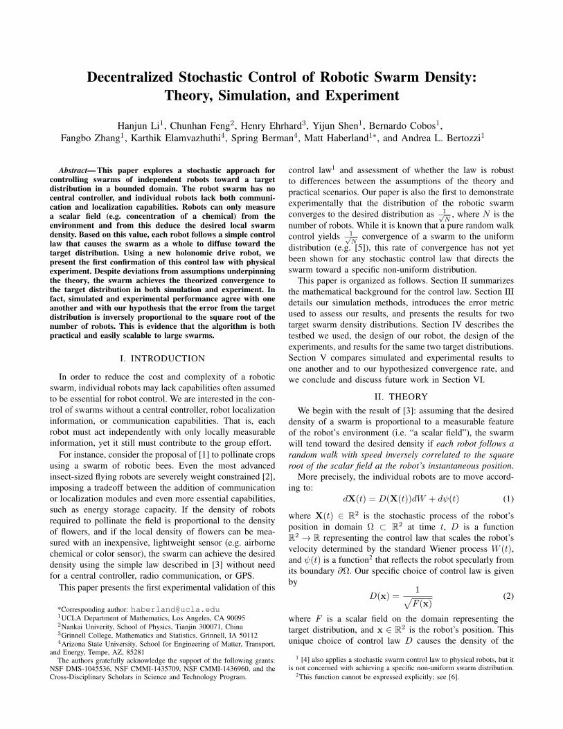
(a) View from above (b) View from bottom

Fig. 4: The Kiwi-drive Robot. For clarity of other compo-nents, identification tag visible in Figure 5 is not shown.

RGB color sensor (TCS34725) fixed to the underside of thechassis, which illuminates the scalar field print with whiteLEDs and measures the red, green, and blue components ofthe reflected light. The robot distinguishes the scalar fieldfrom the boundary by color: black represents a high valueof the scalar field, white represents a low value of the scalarfield, and red represents the boundary.

3) Data Collection: Two overhead cameras record themotion of the robot. We process the video with OpenCV [9]in Python to track the position of the centroid of the robotthrough time. We found the position measured by computervision tracking to be within 2cm of ground measurement fora variety of robot positions throughout the space.

4) Experiment Design: We placed the robot in the speci-fied initial position on top of the scalar field print, startedrecording data with the overhead cameras, and initiatedthe control algorithm on the robot. After 180s5, the videorecording stops automatically, and we manually turned therobot off. This process was repeated 200 times for each ofthe scalar field patterns.

B. Results

In addition to bounded speed and the modified boundarycontrol law, another deviation between the physical robotand theoretical assumptions is imperfect control of velocitydue to limited control signal (PWM) precision, nonlinearresponse of the motors with respect to control signal, wheelslipping, and robot inertia. In spite of this, the ensembleof robot final positions in physical experiment achieves thetarget distribution, and results of physical experiment matchthose of simulation very closely.

Figure 5 depicts the convergence of the ‘swarm’ to thedesired distribution through time-lapse images. Figure 6shows sample configurations and density distributions, asmeasured by the Gaussian blob function of Equation 9,achieved in physical experiment with N = 199 robot runs6

5This was chosen to be 20% longer than the 150s required for steadystate to be achieved in early simulations for the ring pattern. Unfortunately,this was before the maximum speed of the robot was accurately measured,so experiments only capture transient behavior.

6Data from one of the robot runs was found to be invalid after experi-mentation was complete.

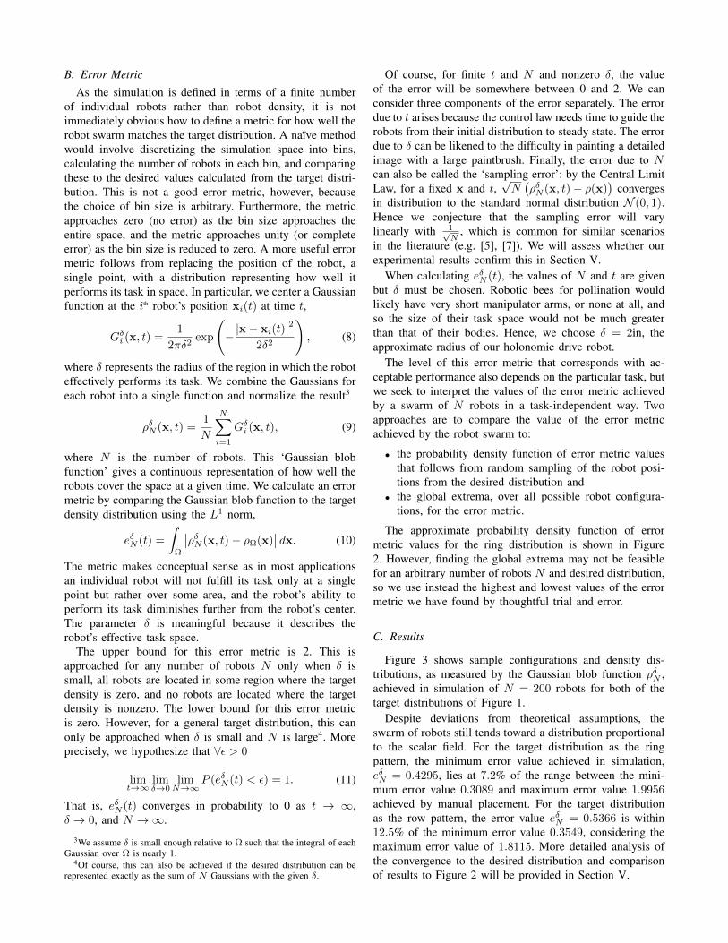
(a) t ≈ 0 s (b) t ≈ 25 s

(c) t ≈ 80 s (d) t ≈ 170 s

Fig. 5: Sample robot configurations for ring target dis-tribution. As results were obtained by running one robot200 times rather than 200 robots once, each frame abovewas produced by sampling a random subset of 50 runs andsuperposing images taken by the overhead cameras duringthose runs. The robot, as seen in Figure 4, is obscured by anidentification tag, visible as a solid black rectangle within awhite rectangle. The thin line outlining the identification tagwas generated in post-processing, and the circular ‘shadow’around each robot is an artifact of the (selective) superposi-tion of multiple images.

for the ring pattern and N = 200 robot runs for the rowpattern. For the target distribution as the ring pattern, theminimum error value achieved in experiment, eδN = 0.4816,lies at 10.2% of the range between the minimum error value0.3089 and maximum error value 1.9956 achieved by manualplacement. For the target distribution as the row pattern, theerror value eδN = 0.6477 is within 20.1% of the minimumerror value 0.3549, considering the maximum error value of1.8115. These error numbers are higher in experiments thansimulation because the experiment did not run for as longas the simulation and did not have a chance to settle intoa steady state. Nonetheless, it is clear that the control law

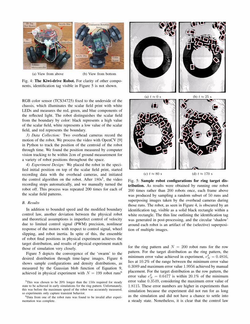
(a) Robot positions at t = 175.5s for ring distribution withN = 199 robots (left) and at t = 160.5s for row distributionwith N = 200 robots (right). The exceptionally careful readerwill note that there are only 198 robot markers on the rowdistribution plot on the right, not 200. This is because in twotrials, the robot was slightly outside the boundary (and in theprocess of ‘bouncing’ back in) when the robot positions wererecorded.

(b) Gaussian blob function ρδ=2inN=199(t = 175.5s) for ring

distribution (left) and ρδ=2inN=200(t = 160.5s) for row distribution

(right).

Fig. 6: Sample results from physical experiment for bothtarget distributions. The times t are those at which the errormetric eδN is minimized. The robot positions and Gaussianblob function show that the control law guides the robotstoward the target distribution. However, the experiments didnot run long enough to achieve steady state. This is partic-ularly apparent for the row distribution as the concentrationin the top right, where all robots began, remains higher thanelsewhere.

tended to produce the desired distribution, and we will showin the following section that experiment agreed remarkablywell with simulation with respect to the transient behavior.

V. DISCUSSION

A. Time Convergence

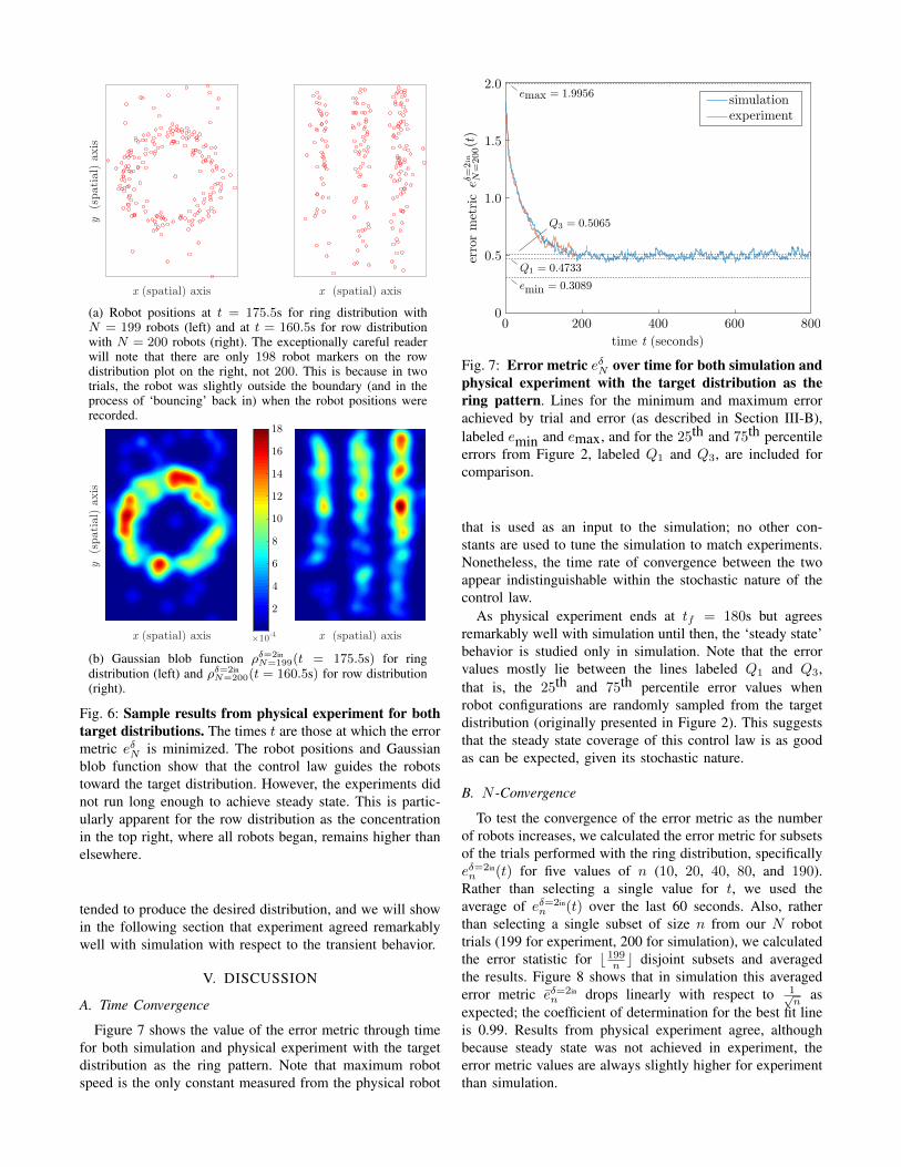
Figure 7 shows the value of the error metric through timefor both simulation and physical experiment with the targetdistribution as the ring pattern. Note that maximum robotspeed is the only constant measured from the physical robot

Fig. 7: Error metric eδN over time for both simulation andphysical experiment with the target distribution as thering pattern. Lines for the minimum and maximum errorachieved by trial and error (as described in Section III-B),labeled emin and emax, and for the 25th and 75th percentileerrors from Figure 2, labeled Q1 and Q3, are included forcomparison.

that is used as an input to the simulation; no other con-stants are used to tune the simulation to match experiments.Nonetheless, the time rate of convergence between the twoappear indistinguishable within the stochastic nature of thecontrol law.

As physical experiment ends at tf = 180s but agreesremarkably well with simulation until then, the ‘steady state’behavior is studied only in simulation. Note that the errorvalues mostly lie between the lines labeled Q1 and Q3,that is, the 25th and 75th percentile error values whenrobot configurations are randomly sampled from the targetdistribution (originally presented in Figure 2). This suggeststhat the steady state coverage of this control law is as goodas can be expected, given its stochastic nature.

B. N -Convergence

To test the convergence of the error metric as the numberof robots increases, we calculated the error metric for subsetsof the trials performed with the ring distribution, specificallyeδ=2inn (t) for five values of n (10, 20, 40, 80, and 190).

Rather than selecting a single value for t, we used theaverage of eδ=2in

n (t) over the last 60 seconds. Also, ratherthan selecting a single subset of size n from our N robottrials (199 for experiment, 200 for simulation), we calculatedthe error statistic for b 199

n c disjoint subsets and averagedthe results. Figure 8 shows that in simulation this averagederror metric eδ=2in

n drops linearly with respect to 1√n

asexpected; the coefficient of determination for the best fit lineis 0.99. Results from physical experiment agree, althoughbecause steady state was not achieved in experiment, theerror metric values are always slightly higher for experimentthan simulation.

Fig. 8: Relationship between the error metric eδn andnumber of robots n (δ = 2in, ring pattern). Note that theerror tends toward a nonzero value as n increases. This isprimarily due to the nonzero δ, as discussed in Section III-B.Nonetheless, the decrease is quite linear with respect to 1√

n,

as expected.

Combined with the time-convergence results, this givesconfidence that the control law is correctly implementedin both simulation and experiment, and furthermore, thatdespite conditions of the theory not being met, the controllaw itself scales to large numbers of robots and is robustenough to work effectively under real-world conditions.

C. Future Work

We have assumed that the robots are small relative tothe environment or that collisions between robots are in-consequential and would not affect the net behavior of theswarm, given its stochastic nature. However, we would liketo consider the case in which collisions must be avoided toprevent damage to the robots. If each robot were equippedwith a rangefinder to sense the relative location of otherrobots, the addition of suitable repulsive “forces” betweenall nearby robots would prevent collision while preservingthe diffusive nature of the swarm. However, we have foundin preliminary simulation that this can slow convergenceto the desired distribution and increase the steady stateerror, especially in regions where high density is desired,so additional work is necessary.

The simulation and experiment have relied on the robotshaving a holonomic drive system, that is, the robot cantranslate in any direction independent of orientation. Ap-plication of the control algorithm to non-holonomic robots,such as those that steer like tanks or cars, may be relativelystraightforward: the average velocity of the robot during atime step is calculated as for the holonomic robot, but apath to the destination defined by the average velocity mustbe planned. We have performed simulation and preliminaryphysical experiments with a tank-drive robot that simplyrotates toward the destination before following a straight-line path to it, but additional work is required to confirmthat this is the most efficient approach.

While this control law might be sufficient to drive robotbees close to target flowers, robots would need to switchto a different control law, such as that of [10], to land onflowers and perform pollination work. Future work includesimplementing robot behavioral switches between “active”(flying) and “passive” (pollinating) states.

Note that theory regarding convergence of the control lawis valid even when the desired distribution is not binary.In preliminary simulations with a smoothly varying scalarfield, the algorithm still seems robust. The controller is alsovalid when the robot cannot sense a scalar field from itsenvironment directly, but instead knows its own location andthus the corresponding value of a pre-assigned scalar field.For example, the strategy could be used for public safetyoperations in which robots patrol with density proportionalto a known or expected threat. These possibilities should betested in future experiments.

VI. CONCLUSION

We have presented experimental validation of simple,decentralized, stochastic control law that guides a swarmof entirely independent robots toward a desired distribution.Despite significant discrepancies between the experimentalplatform and the theoretical assumptions upon which thecontroller is based, the swarm achieves the desired distribu-tion in practice at time rates comparable to simulation. Theexperimental results even show that the asymptotic error ofthe swarm is proportional to 1√

N, where N is the number

of robots, as hypothesized. This performance and robustnesssuggest that the control law would be an effective choice fordistributing large swarms of inexpensive robots with limitedsensing and no communication or localization abilities.

REFERENCES

[1] S. Berman, V. Kumar, and R. Nagpal, “Design of control policiesfor spatially inhomogeneous robot swarms with application to com-mercial pollination,” in Robotics and Automation (ICRA), 2011 IEEEInternational Conference on. IEEE, 2011, pp. 378–385.

[2] K. Y. Ma, P. Chirarattananon, S. B. Fuller, and R. J. Wood, “Controlledflight of a biologically inspired, insect-scale robot,” Science, vol. 340,no. 6132, pp. 603–607, 2013.

[3] K. Elamvazhuthi, C. Adams, and S. Berman, “Coverage and field esti-mation on bounded domains by diffusive swarms,” in IEEE Conferenceon Decision and Control (CDC), Las Vegas, NV, 2016, pp. 2867–2874.

[4] A. Prorok, N. Correll, and A. Martinoli, “Multi-level spatial modelingfor stochastic distributed robotic systems,” International Journal ofRobotics Research, vol. 30, no. 5, pp. 574–589, 2011.

[5] P. Szymczak and A. Ladd, “Boundary conditions for stochastic solu-tions of the convection-diffusion equation,” Physical review E, vol. 68,no. 3, p. 036704, 2003.

[6] H. Tanaka et al., “Stochastic differential equations with reflectingboundary condition in convex regions,” Hiroshima Mathematical Jour-nal, vol. 9, no. 1, pp. 163–177, 1979.

[7] G. A. Pavliotis, Stochastic processes and applications, ser. Texts inApplied Mathematics. Springer-Verlag, 2014.

[8] R. Rojas and A. G. Forster, “Holonomic control of a robot with anomnidirectional drive,” KI-Kunstliche Intelligenz, vol. 20, no. 2, pp.12–17, 2006.

[9] Itseez, “Open source computer vision library,” http://www.opencv.org/,2015.

[10] M. Graule, P. Chirarattananon, S. Fuller, N. Jafferis, K. Ma,M. Spenko, R. Kornbluh, and R. Wood, “Perching and takeoff of arobotic insect on overhangs using switchable electrostatic adhesion,”Science, vol. 352, no. 6288, pp. 978–982, 2016.