Decentralized Information Processing in Wireless Peer-to

University of California

Los Angeles

Decentralized Information Processing in

Wireless Peer-to-Peer Networks

A dissertation submitted in partial satisfaction

of the requirements for the degree

Doctor of Philosophy in Electrical Engineering

by

Mohiuddin Ahmed

2002

c© Copyright by

Mohiuddin Ahmed

2002

The dissertation of Mohiuddin Ahmed is approved.

Izhak Rubin

Kung Yao

Mario Gerla

Gregory J. Pottie, Committee Chair

University of California, Los Angeles

2002

ii

To my parents.

iii

Table of Contents

1 Introduction . . . . . . . . . . . . . . . . . . . . . . . . . . . . . . . . 1

1.1 Information Processing in Wireless Networks . . . . . . . . . . . . 1

1.2 Thesis Topics and Contributions . . . . . . . . . . . . . . . . . . . 4

2 Distributed Data Fusion in Sensor Networks: An Information

Processing Approach . . . . . . . . . . . . . . . . . . . . . . . . . . . . 9

2.1 Introduction . . . . . . . . . . . . . . . . . . . . . . . . . . . . . . 9

2.1.1 Evolution Towards Multi-Sensor Systems . . . . . . . . . . 13

2.1.2 An Information Processing Approach to Sensor Networks . 18

2.2 A Bayesian Scheme for Decentralized Data Fusion . . . . . . . . . 20

2.2.1 Sensor Data Model for Single Sensors . . . . . . . . . . . . 20

2.2.2 Bayesian Estimation and Inference . . . . . . . . . . . . . 24

2.2.3 Classical Estimation Techniques . . . . . . . . . . . . . . . 27

2.2.4 Sensor Data Model for Multi-Sensor Systems . . . . . . . . 29

2.3 Information Theoretic Justification of the Bayesian Method . . . . 34

2.3.1 Information Measures . . . . . . . . . . . . . . . . . . . . . 35

2.4 Multi-Sensor Data Fusion Architectures . . . . . . . . . . . . . . . 38

2.4.1 Classification of Sensor Network Architectures . . . . . . . 38

2.4.2 An Architecture for Likelihood Opinion Pool Data Fusion . 44

2.5 Concluding Remarks . . . . . . . . . . . . . . . . . . . . . . . . . 47

3 Some Information Processing Bounds in Data Networks . . . . 49

iv

3.1 Rate Distortion of n-Helper Gaussian Sources . . . . . . . . . . . 50

3.1.1 Analytic Formulation . . . . . . . . . . . . . . . . . . . . . 53

3.1.2 Conclusion . . . . . . . . . . . . . . . . . . . . . . . . . . . 57

3.2 Asymptotic Delay in Random Wireless Networks . . . . . . . . . 58

3.2.1 Introduction . . . . . . . . . . . . . . . . . . . . . . . . . . 58

3.2.2 Analysis . . . . . . . . . . . . . . . . . . . . . . . . . . . . 60

3.2.3 Concluding Remarks . . . . . . . . . . . . . . . . . . . . . 63

4 Gateway Optimization for Connectivity in Heterogeneous Multi-

Tiered Wireless Networks . . . . . . . . . . . . . . . . . . . . . . . . . 64

4.1 Introduction . . . . . . . . . . . . . . . . . . . . . . . . . . . . . . 65

4.2 System Model . . . . . . . . . . . . . . . . . . . . . . . . . . . . . 67

4.3 CCA Trajectory Update Algorithm: Formulation and Analysis . . 70

4.3.1 Node Domains Containing a Single CCA . . . . . . . . . . 71

4.3.2 Overlapping CCA Domains . . . . . . . . . . . . . . . . . 76

4.4 Computational Complexity and Overhead . . . . . . . . . . . . . 80

4.4.1 MAC Protocol, Routing Support and Overhead . . . . . . 80

4.4.2 Optimization Complexity . . . . . . . . . . . . . . . . . . 82

4.5 Simulation Framework and Results . . . . . . . . . . . . . . . . . 83

4.6 Conclusions . . . . . . . . . . . . . . . . . . . . . . . . . . . . . . 93

5 Dependability of Wireless Heterogeneous Networks . . . . . . . 95

5.1 Introduction . . . . . . . . . . . . . . . . . . . . . . . . . . . . . . 96

5.2 Graph Theory Fundamentals for Modeling Ad Hoc Networks . . . 99

v

5.2.1 Deterministic Graphs . . . . . . . . . . . . . . . . . . . . . 100

5.2.2 Probabilistic Graphs and Reliability Measures . . . . . . . 106

5.3 Dependability Optimization for Node Failures . . . . . . . . . . . 110

5.3.1 Distributed Node Resilience Criteria (DNRC) for Peer-to-

Peer Networks . . . . . . . . . . . . . . . . . . . . . . . . . 111

5.3.2 Simulation Study of the DNRC Metric . . . . . . . . . . . 115

5.3.3 Optimization of Networks Using DNRC Metric, γ(G)—a

Design Flow . . . . . . . . . . . . . . . . . . . . . . . . . . 118


5.4 Case Study: Dependability Protocols for the NGI Network . . . . 120

5.4.1 Dependability of the NGI Architecture . . . . . . . . . . . 121

5.4.2 Prior Research . . . . . . . . . . . . . . . . . . . . . . . . 125

5.4.3 Failure Recovery Modes for Gateways in Hybrid Network . 126

5.4.4 Algorithms for NGI Gateway Fault Tolerance and Security 130

5.4.5 Implementation of the Gateway Reliability Algorithms . . 137


5.4.7 Flowcharts and Figures . . . . . . . . . . . . . . . . . . . . 140

6 Rate Adaptive MIMO OFDM LDPC transceiver . . . . . . . . 152

6.1 Introduction . . . . . . . . . . . . . . . . . . . . . . . . . . . . . . 153

6.2 Primer on MIMO, OFDM and LDPC . . . . . . . . . . . . . . . . 156

6.2.1 Multiple Input, Multiple Output (MIMO) Systems . . . . 156

6.2.2 Orthogonal Frequency Domain Multiplexing (OFDM) . . . 160

6.2.3 Low Density Parity Check (LDPC) Channel Codes . . . . 164

vi

6.3 MIMO-OFDM Channel Estimation . . . . . . . . . . . . . . . . . 171

6.3.1 Simplified Channel Estimation for LDPC coded MIMO-

OFDM Channels: Code Design . . . . . . . . . . . . . . . 174

6.3.2 Channel Matrix Estimation . . . . . . . . . . . . . . . . . 180

6.4 Combining LDPC and OFDM with MIMO . . . . . . . . . . . . . 181

6.4.1 Likelihood Metrics for OFDM modulated LDPC . . . . . . 181

6.4.2 MIMO Signal Separation . . . . . . . . . . . . . . . . . . . 183

6.4.3 LDPC Soft Bit-Metrics for Decoding M-ary Symbols in

OFDM . . . . . . . . . . . . . . . . . . . . . . . . . . . . . 186

6.5 Adaptivity for LDPC coded MIMO-OFDM and System Design . . 188

7 Conclusion . . . . . . . . . . . . . . . . . . . . . . . . . . . . . . . . . 194

7.1 Future Directions . . . . . . . . . . . . . . . . . . . . . . . . . . . 195

References . . . . . . . . . . . . . . . . . . . . . . . . . . . . . . . . . . . 199

vii

List of Figures

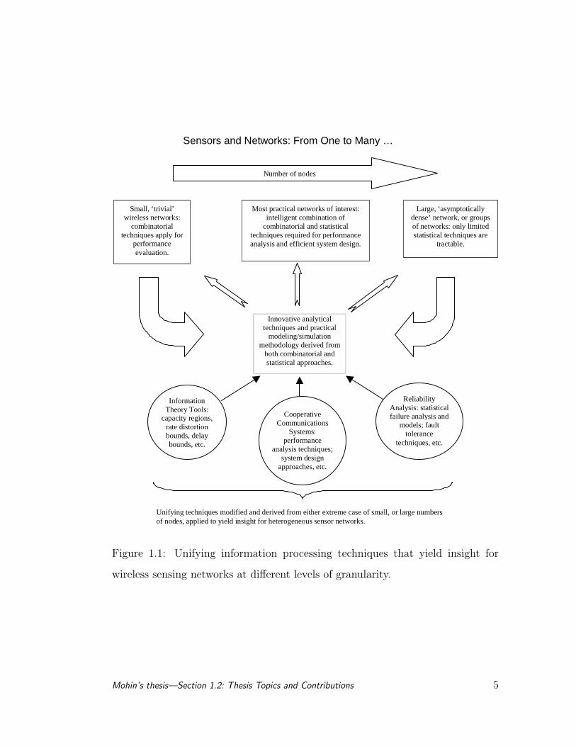
1.1 Unifying information processing techniques that yield insight for

wireless sensing networks at different levels of granularity. . . . . . 5

2.1 Information Processing in Sensors . . . . . . . . . . . . . . . . . . 10

2.2 Information Processing in Distributed Sensors . . . . . . . . . . . 13

2.3 Sensor data models: (i) General case (ii) Noise additive case. . . . 23

2.4 Ellipsoid of state vector uncertainty . . . . . . . . . . . . . . . . . 25

2.5 Multi-Sensor Data Fusion by Linear Opinion Pool . . . . . . . . . 31

2.6 Multi-Sensor Data Fusion by Independent Opinion Pool . . . . . . 32

2.7 Multi-Sensor Data Fusion by Likelihood Opinion Pool . . . . . . . 34

2.8 Centralized Data Fusion Architecture . . . . . . . . . . . . . . . . 39

2.9 Hierarchical Data Fusion Architecture . . . . . . . . . . . . . . . . 41

2.10 Decentralized Data Fusion Architectures: (i) Fully Connected (ii)

Arbitrary . . . . . . . . . . . . . . . . . . . . . . . . . . . . . . . 43

2.11 Likelihood Information Processing for Single Sensors . . . . . . . 45

2.12 Architecture for Multi-sensor Data Fusion using Likelihood Opin-

ion Pool . . . . . . . . . . . . . . . . . . . . . . . . . . . . . . . . 47

3.1 Wireless Integrated Network Sensor System . . . . . . . . . . . . 52

3.2 Data Fusion for a Wireless Networked Sensor System . . . . . . . 53

4.1 Ad hoc network of two groups of mobile nodes and CCAs. . . . . 68

4.2 CCA domain with location bounds. . . . . . . . . . . . . . . . . . 72

viii

4.3 Overlapping CCA domains . . . . . . . . . . . . . . . . . . . . . . 77

4.4 Comparison of network throughput with optimally placed CCA

versus statically placed or randomly moving CCA. . . . . . . . . . 86

4.5 Effect of blockages on the performance of the static vs. optimally

placed CCAs. . . . . . . . . . . . . . . . . . . . . . . . . . . . . . 87

4.6 Comparison of CCA optimization calculations with/without the

effect of loading parameters. . . . . . . . . . . . . . . . . . . . . . 88

4.7 The effect of loading on latency of transmitted data packets for

the static and dynamically placed CCAs . . . . . . . . . . . . . . 89

4.8 Effect of including the effect of priority in the optimization cost

function. . . . . . . . . . . . . . . . . . . . . . . . . . . . . . . . . 90

4.9 Comparison of CCA loads with and without having a method to

balance loads when domains intersect. . . . . . . . . . . . . . . . 92

5.1 A pictorial representation of a graph (algebraic) structure . . . . . 101

5.2 Representation of an Ad Hoc Network with Symmetric Links . . . 102

5.3 Isomorphic Graphs . . . . . . . . . . . . . . . . . . . . . . . . . . 103

5.4 γ(G) Calculation for a Simple Network. . . . . . . . . . . . . . . . 114

5.5 Flowchart for CCA or ‘Aggregation’ Node Local Computation for

Optimizing Reliability . . . . . . . . . . . . . . . . . . . . . . . . 119

5.6 NGI Architecture and Failure Points . . . . . . . . . . . . . . . . 121

5.7 Flowchart for mobile initiated reactive fault-tolerance scheme . . . 146

5.8 Flowchart for mobile initiated proactive fault-tolerance scheme . . 147

5.9 Flowchart for gateway initiated, reactive fault-tolerance scheme . 148

ix

5.10 Flowchart for gateway initiated, proactive fault-tolerance scheme. 148

5.11 Secure gateway selection algorithm. . . . . . . . . . . . . . . . . . 149

5.12 Node/gateway layout used for testing fault-tolerance algorithms. . 149

5.13 Overall throughput in best basestation vs. round-robin gateway

selection algorithms for the DSDV routing protocol, as a function

of number of gateways in domain. . . . . . . . . . . . . . . . . . . 150

5.14 Overall throughput in best basestation vs. round-robin gateway

selection algorithms for DSR routing protocol, as a function of

number of gateways in domain. . . . . . . . . . . . . . . . . . . . 151

6.1 Block diagram of proposed MIMO-OFDM-LDPC transceiver. . . 155

6.2 MIMO transceiver in the presence of RF scatters. . . . . . . . . . 158

6.3 Capacity potential for MIMO transceivers in RF cluttered envi-

ronment. . . . . . . . . . . . . . . . . . . . . . . . . . . . . . . . . 158

6.4 OFDM time and frequency domain waveforms. . . . . . . . . . . . 163

6.5 OFDM transmitter/receiver block diagram. . . . . . . . . . . . . . 164

6.6 Tanner graph of LDPC code parity check matrix. . . . . . . . . . 169

6.7 Likelihood ratio decoding of LDPC codes. . . . . . . . . . . . . . 171

6.8 Multi-input, multi-output radio frequency channel. . . . . . . . . 174

6.9 Three-tap FIR filter model for a 2× 1 MIMO channel. . . . . . . 175

6.10 Orthogonal training sequence elements . . . . . . . . . . . . . . . 178

6.11 Autocorrelation of length-6 perfect sequence training symbols. . . 179

6.12 LDPC coded OFDM for a 1× 1 system with 16 OFDM carriers. . 181

6.13 Adaptive OFDM to increase spectral efficiency in IEEE 802.11a. . 189

x

6.14 MIMO-OFDM-LDPC transmitter block diagram. . . . . . . . . . 191

6.15 MIMO-OFDM-LDPC receiver block diagram. . . . . . . . . . . . 191

6.16 Data packet structure. . . . . . . . . . . . . . . . . . . . . . . . . 192

6.17 Simulation results: SISO bounds. . . . . . . . . . . . . . . . . . . 192

6.18 Simulation results: effects of LDPC-OFDM. . . . . . . . . . . . . 193

xi

List of Tables

5.1 DNRC and Connectivity Probability Results for Random Net-

works. . . . . . . . . . . . . . . . . . . . . . . . . . . . . . . . . . 117

5.2 Overhead Requirements for Gateway Fault Tolerance Algorithms. 134

xii

Acknowledgments

It is with deep gratitude, that I acknowledge the guidance, support and encour-

agement provided to me by my advisor, Professor Gregory Pottie. His insight,

assistance, enthusiasm, and flexibility have enabled me to complete an endeavor

I could not have accomplished otherwise.

I would like to thank the members of my dissertation committee: Dr. Mario

Gerla, Dr. Izhak Rubin and Dr. Kung Yao, who have kindly taken the time and

effort to be a part of this process. I am especially grateful to all my teachers

at UCLA, who have provided the most stimulating and rewarding intellectual

experience that I have yet experienced. I only hope that I can do justice to all

that they have taught me.

My appreciation also goes to my supervisors at HRL Laboratories, Dr. Bo Ryu

and Son Dao, who were most considerate and provided me with an opportunity

to pursue my doctoral studies, amidst my responsibilities at HRL.

Most of all, it is with great pride that I acknowledge the fundamental role that

my parents and my family have played in shaping all that I have accomplished in

life. It is to them that I dedicate this work. Finally, words are not adequate to

express the joy and gratitude that I feel towards my wonderful wife, Moonmoon.

Without her patience, support and understanding...well, I’d just rather not think

about it.

xiii

Vita

Publications

Mohiuddin Ahmed and Gregory Pottie, “Information Theory of Wireless Sen-

sor Networks—the n-Helper Gaussian Case,” IEEE International Symposium on

Information Theory (ISIT), Sorrento, Italy, July 2000.

Mohiuddin Ahmed, Yung-Szu Tu and Gregory Pottie, “Cooperative Detection

and Communication in Wireless Sensor Networks,” 38th Annual Allerton Con-

ference on Communication, Control and Computing, Urbana, IL, October 4-6,

2000.

Mohiuddin Ahmed, S. Krishnamurthy, S. Dao, and Gregory Pottie “On the

Optimal Selection of Nodes to Perform Data Fusion in Wireless Sensor Networks,”

Proceedings of the International Society of Optical Engineering (SPIE), Special

Session on Battlespace Digitization and Network Centric Warfare, Orlando, FL,

April 2001.

Mohiuddin Ahmed, Son Dao and Randy Katz, “Performance Issues in Using Mo-

bile communication Agents in Hybrid Satellite/Mobile Ad Hoc Networks,” IEEE

xiv

Military Communications Conference (MILCOM), Tysons Square, VA, October

2001.

Mohiuddin Ahmed and Gregory Pottie, “Asymptotic Delay in Random Wire-

less Networks,” IEEE International Symposium on Information Theory (ISIT),

Lausanne, Switzerland, July 2002.

Mohiuddin Ahmed, S. Krishnamurthy, S. Dao, and R. Katz “Trajectory Con-

trol of Mobile Gateways for Range Extension in Ad Hoc Networks,” Journal of

Computer Networks (Elsevier), Volume 39, Issue 6, August 21, 2002.

xv

Abstract of the Dissertation

Decentralized Information Processing in

Wireless Peer-to-Peer Networks

by

Mohiuddin Ahmed

Doctor of Philosophy in Electrical Engineering

University of California, Los Angeles, 2002

Professor Gregory J. Pottie, Chair

Decentralized information processing systems, such as wireless sensor networks,

facilitate the acquisition, processing and dissemination of information. With the

phenomenal growth in the development of digital hardware and wireless infor-

mation technologies, the efficient handling of data in such systems has become

of prime concern. This thesis deals with several inter-related problems relating

to the processing of information in wireless peer-to-peer networks. It presents

a collection of analysis, algorithmic techniques and results that are designed to

optimize performance in such decentralized systems.

Sensors architectures are analyzed as the starting point of the study, and a

unified, probabilistic, information processing approach to data fusion is presented

for heterogeneous, multi-sensor networks. A likelihood metric aggregation archi-

tecture, based on the Bayesian approach, is highlighted as the central unifying

technique for decentralized organization and interpretation of information. The

need for fundamental performance limits for decentralized networks is then dis-

cussed, and some bounds are derived. In particular, the rate distortion region for

a sensor fusion network with n-helper nodes in a Gaussian setting is described.

xvi

The asymptotic delay order for data packets in a random wireless network is also

derived.

Next, some practical issues dealing with the administration of wireless re-

sources in heterogeneous, multi-tiered ad hoc networks are discussed. A hybrid,

gateway-based architecture and trajectory control algorithms for enabling range

extended connectivity are presented. The dependability for such networks are

then analyzed, and a distributed reliability algorithm is formulated that can be

applied to optimize the dependability of decentralized, dynamic peer-to-peer net-

works. Specific fault tolerance algorithms for the gateway-based architecture are

also devised.

Finally, bandwidth efficient techniques are analyzed that serve to extract the

maximum spectral efficiency in point-to-point communications. A rate adaptive

transceiver is designed that combines multi-input, multi-out (MIMO) antennas,

orthogonal frequency domain multiplexing (OFDM) and low density parity check

(LDPC) channel codes. Channel estimation and novel signal separation tech-

niques are derived.

The overall goal is thus to develop a set of cross layer techniques, from the

physical to the network layer, that can be applied to quantify some of the basic

performance limits for distributed information processing systems.

xvii

CHAPTER 1

Introduction

1.1 Information Processing in Wireless Networks

The last few decades have witnessed a phenomenal growth in the research and

development of solid-state, digital communications, computing and signal pro-

cessing technologies. A beneficial aspect of all this concentrated activity has

been the symbiotic convergence and amalgamation of various hardware, software

and ‘concept-driven’ technologies. This approach, for example, has yielded most

of the information processing devices that we take for granted today. Ostensibly,

the purpose of all this activity has been to improve the human condition; but

from a scientific and engineering point of view, the common unifying purpose

that has shaped and guided the general research direction in these disciplines has

been the desire to acquire, manipulate, and disseminate information. In the same

vein, this thesis focuses on some inter-related problems of information processing.

In particular, the ability to electronically network together what were previ-

ously isolated islands of information sources and sinks has revolutionized many

research disciplines. One such effort has been in the cooperative sensing and

control of the environment (or more generally, states of nature). This can re-

fer to measurements of physical parameters (e.g. temperature, humidity, etc.)

or estimates of operational conditions (network loads, throughput, etc.), among

other things. Previously, these activities were performed by isolated sensors, re-

1

quiring human supervision and control. However, with the advent of powerful

hardware platforms and networking technologies, the possibility and advantages

of distributed sensing has been recognized. Inspite of the advances in sensor

technologies and the many computational methods and algorithms aimed at ex-

tracting information from a given sensor/actuator, the fact remains that no single

sensor is capable of obtaining a required state information reliably, at all times, in

different and sometimes dynamic environments. Furthermore, it has been estab-

lished from the theory of distributed detection that higher reliability and lower

probability of detection error can be achieved when observation data from mul-

tiple, distributed sources is intelligently fused in a decision making algorithm,

rather than using a single observation data set. The main advantages of using

networked, multi-system platforms can thus be summarized as follows.

• Reliability and greater accuracy through redundancy, by using multiple

sensors to measure the same or overlapping quantities, and exploiting the

fact that the signal relating to the observed quantity is correlated whereas

the uncertainty associated with each sensor is uncorrelated.

• Diversity, where physical sensor diversity uses different sensor technologies

together, and spatial diversity offers differing viewpoints of the sensor en-

vironment.

• Scalability, where decisions can be made over a larger state space of obser-

vations by having distributed, efficient local computations and hierarchical

data fusion, thereby reducing the complexity of the command and control

center’s operations.

These issues are especially notable in the context of heterogeneous sensor/-

actuator nodes. These devices may be networked or as part of larger mobile

Mohin’s thesis—Section 1.1: Information Processing in Wireless

Networks 2

platforms, forming an ad hoc network of wireless integrated information pro-

cessing devices. Their function is to engage in cooperative, distributed sensing,

computation, and communications for decision and action. However, there are

significant research and engineering issues that need to be addressed before such

heterogeneous systems can be successfully deployed, and these problems are cur-

rently at the scientific frontiers of Information Technology.

Focus of the thesis:

In this thesis, the above mentioned issues are studied in the context of the

following general problem: given a multiplicity of wireless sensors, and a sens-

ing/processing objective, what is the optimum set of tasks to—

(i) efficiently extract as much information as possible about a sensed environ-

ment;

(ii) process the data locally, and/or intelligently fuse the aggregate data at

distributed hierarchical levels, according to the sensing objectives;

(iii) cooperate to maintain connectivity and interact with command and control

centers for communicating decision variables and instructions.

The assumption is made of a system of heterogeneous sensor (or general ad

hoc) networks, working cooperatively for a particular sensing objective. This

distributed information processing approach can overcome the shortcomings of

the alternative approach of using a highly sophisticated, but single sensor for the

same objective. But, as noted above, the effective deployment of such distributed

processing systems introduces some significant design issues, most notably: scala-

bility, networking and communication protocols, transmission channel and power

constraints, reliability, among others. The approach taken in this thesis is to

Mohin’s thesis—Section 1.1: Information Processing in Wireless

Networks 3

study these issues from several different viewpoints: information theoretic; data

fusion and reliability based; and from practical cooperative, rate adaptive, ef-

ficient digital communications considerations. The objective is to gain insight

into novel paradigms for the data fusion and performance analysis of networked

sensors; for evaluating the asymptotic rate and delay properties of such random

networks; for the architectures necessary for ad hoc structures involving a het-

erogeneous mix of such sensors, their reliability and fault tolerance issues, etc.,

and finally we also look at bandwidth efficient techniques that can be used for

such distributed information processing systems.

One of the unifying features that is common to these approaches is the analysis

of factors that affect performance when scaling the number of nodes in a sensor

system from a few (when combinatorial methods for system performance may be

tractable) to many (when statistical methods are the only options). The goal is to

thus to determine these intelligent unifying techniques, approaching the problem

from these varying analysis viewpoints: to quantify, analyze and understand the

answers to some of the basic architectural and performance limits questions for

distributed sensing systems. We have attempted to envision this philosophy as

depicted in Figure 1.1.

1.2 Thesis Topics and Contributions

In this thesis, the following five topics relating to information processing in wire-

less peer-to-peer networks are studied, in the order listed. A summary of the

contributions that have been made in each topic is provided below, and the de-

tailed accounts are presented as Chapters 2 through 6 of this thesis.

1. Data Fusion: This is the problem of combining diverse and sometimes

Mohin’s thesis—Section 1.2: Thesis Topics and Contributions 4

Small, ‘ trivial’ wireless networks:

combinatorial techniques apply for

performance evaluation.

Large, ‘asymptotically dense’ network, or groups of networks: only limited statistical techniques are

tractable.

Most practical networks of interest: intelligent combination of

combinatorial and statistical techniques required for performance analysis and efficient system design.

Innovative analytical techniques and practical

modeling/simulation methodology derived from

both combinatorial and statistical approaches.

Unifying techniques modified and derived from either extreme case of small, or large numbers of nodes, applied to yield insight for heterogeneous sensor networks.

Number of nodes

Information Theory Tools:

capacity regions, rate distortion bounds, delay bounds, etc.

Cooperative Communications

Systems: performance

analysis techniques; system design

approaches, etc.

Reliability Analysis: statistical failure analysis and

models; fault tolerance

techniques, etc.

Sensors and Networks: From One to Many …

Figure 1.1: Unifying information processing techniques that yield insight for

wireless sensing networks at different levels of granularity.


conflicting information provided by sensors in a multi-sensor system, in a

consistent and coherent manner. The objective is to infer the relevant states

of the system that is being observed or activity being performed. Using

probabilistic and decision theoretic principles, this thesis presents a unified

treatment of information processing, within the framework of the Bayesian

Paradigm, as they relate to the issues of: data representation, fusion, and

transmission in decentralized sensor networks. It is shown in Chapter 2

of this thesis that the core elements of decentralized, heterogeneous data

fusion can be quantitatively formulated and analyzed using a generalized,

modular information processing framework that is amenable to practical

implementation.

2. Information Theoretic Bounds: This relates to results that delineate

the boundaries of the amount of information processing that can be done

with multi-terminal networks. It is evident that some fundamental limits

are required to assess the optimality of any system design with regard to

the “best design”, given the available resources for a particular application.

Unfortunately, comprehensive general information theories do not yet exist

for decentralized, multi-terminal networks. So, in Chapter 3 of the thesis,

some simplified asymptotic cases are studied. In particular, wireless sensor

networks and the data fusion process are modeled from a classical infor-

mation theoretic viewpoint, and the rate distortion region for correlated

sources is derived for a special case. Most practical sensor and ad hoc net-

works are also too large for combinatorial or queueing theory analysis to

determine fundamental properties such as end-to-end throughput and de-

lay. In this regard, also in this chapter, a simplified scenario is considered,

and based on recent results, the asymptotic delay order that is experienced


by an ‘average’ data packet in the network is derived.

3. Resource Administration—the NGI framework: This relates to the

task of optimally configuring, coordinating and utilizing available sensor

and ad hoc resources, often in a dynamic, adaptive environment. The

objective is to ensure efficient1 use of the wireless resources for the task at

hand. In Chapter 4 of this thesis, this problem is approached in the context

of a hybrid, multi-tiered network that is envisioned to be the architecture

for the Next Generation Internet.2 In particular, the role of mobile gate-

ways is recognized as crucial in enabling cross-platform connectivity and

managing fusion/relay processes (as in Chapter 2), and the resulting archi-

tectural implications are critically examined. Protocols are developed for

the optimal trajectory control of gateways, and for load-balancing, etc.

4. Dependability of Heterogeneous Networks: Heterogeneous networks

often rely on special network architectural arrangements for information

processing (e.g. hierarchical or centralized nodes, defined backbone pro-

tocols, etc.). However, this also causes such networks to suffer a greater

vulnerability due to faults and failures among its critical nodes. The focus

of Chapter 5 of the thesis is to use graph theoretic techniques to analyze the

dependability of heterogeneous wireless ad hoc networks. This approach is

then used to yield insight into how to improve network protocols that can

lead to more dependable systems. Detailed protocols are developed to opti-

mize moderately sized networks against node and link failures, and several

algorithms are developed to handle the specific case of gateways in the NGI

1Efficiency, in this context, is very general and can refer to power, bandwidth, over-head, throughput, or a variety of other performance metrics, depending upon the particularapplication.

2DARPA NGI project, http://www.darpa.mil/ipto/research/ngi.


context.

5. Bandwidth efficient communications using MIMO-OFDM-LDPC

transceivers: With the exponential rise in the use of wireless systems,

it has become increasingly important to extract the maximum diversity

from the time, space and frequency dimensions in which radio frequency

devices operate. The final chapter of the thesis (Chapter 6) deals with

this physical layer issue for hybrid wireless networks, by proposing a novel

approach that maximizes the raw spectral efficiency of transceivers. This is

accomplished by using a combination of three recent developments in digital

communication theory to form a space-time coded transceiver that can be

adaptively optimized. These technologies are: multi-input, multi-output

antenna technology (MIMO), orthogonal frequency domain multiplexing

(OFDM), and the powerful low density parity check channel codes (LDPC).

In this thesis, in particular, novel signal separation and channel estimation,

as well as adaptive modulation schemes are suggested.

The research effort that is the subject matter of this thesis thus deals with

several inter-related problems relating to the processing of information in wireless

networks, and presents a collection of analysis, algorithmic techniques, and results

that are designed to optimize performance in hybrid peer-to-peer networks. The

detailed descriptions follow.


CHAPTER 2

Distributed Data Fusion in Sensor Networks:

An Information Processing Approach

2.1 Introduction

Sensors, in the context of this thesis, refer to physical devices that exploit physical

phenomena to measure quantities. A sensor can be defined to be any device that

provides a quantifiable set of outputs in response to a specific set of inputs. Usu-

ally, the inputs are environmental or physical parameters of interest in natural or

artificial systems, and the outputs are measurable attributes of those parameters.

So, for example, a temperature sensor registers the temperature, a gas pressure

sensor senses pressure values, and so on. Sensors can also be software algorithms,

e.g. subroutines measuring the data load through routers, diagnostic subroutines

monitoring the status of devices, etc.1

Sensors are expected to provide information about the state of nature. A

particular sensor device is considered appropriate for a sensing task when a re-

lationship or mapping exists between the measured quantity and the state of

nature. The end goal of the sensing task is to acquire a description of the ex-

ternal world, predicated upon which can be a series of actions. For example,

velocity sensors in an automobile report the speed of the vehicle, which the oper-

1Natural biological sensing systems, such as our eyes, ears, etc., and other types of sensingmethodologies based on behaviorial, psychological metrics, etc. are not considered in this thesis.

9

ator of the vehicle then adjudges to perform some action (accelerate, decelerate,

or maintain constant speed).

Typically, in devices to date, sensors have been integrated as part of larger,

more complex systems are have designed for specific purposes. So, whether the

objective has been to land a person on the moon, or to enable a vehicle to travel

from a particular point to another point in space, the sensors on board such

devices provide a variety of state information that the system/operator then

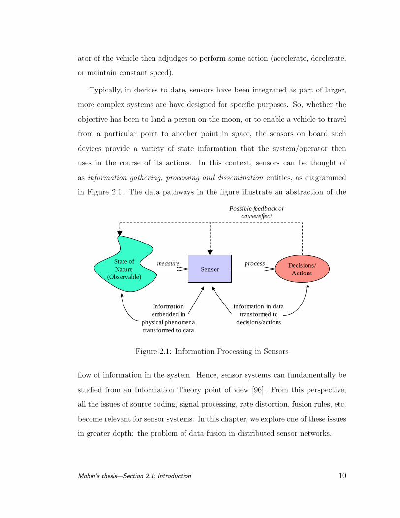
uses in the course of its actions. In this context, sensors can be thought of

as information gathering, processing and dissemination entities, as diagrammed

in Figure 2.1. The data pathways in the figure illustrate an abstraction of the

SensorDecisions/

Actions

State ofNature

(Observable)

measure process

Information embedded in

physical phenomena transformed to data

Information in data transformed to

decisions/actions

Possible feedback or cause/effect

Figure 2.1: Information Processing in Sensors

flow of information in the system. Hence, sensor systems can fundamentally be

studied from an Information Theory point of view [96]. From this perspective,

all the issues of source coding, signal processing, rate distortion, fusion rules, etc.

become relevant for sensor systems. In this chapter, we explore one of these issues

in greater depth: the problem of data fusion in distributed sensor networks.

Mohin’s thesis—Section 2.1: Introduction 10

Rather than using single sensor platforms, modern sensor system hardware

architectures often integrate multiple sensors that are physically disjoint or dis-

tributed in time or space, and that work cooperatively (an example of a dis-

tributed-parameter rather than a lumped-parameter system [10]). The extra di-

mensions and distributed nature of these systems add layers of complexity in

the information gathering, processing and dissemination tasks, and is the central

focus of this thesis.

The reasons for having a network of sensors, as opposed to a single sensor

platform, essentially reduce to the advantages of diversity. Any practical sens-

ing device has limitations on its sensing capabilities (e.g. resolution, bandwidth,

efficiency, etc.). The primary limitation is that descriptions or physical models

built on the data sensed by a device are, unavoidably, only approximations of

the true state of nature. Such approximations are often made worse by incom-

plete knowledge and understanding of the environment that is being sensed and

its interaction with the sensor. These uncertainties, coupled with the practical

reality of occasional sensor failure greatly compromises reliability and reduces

confidence in sensor measurements. Also, the spatial and physical limitations of

sensor devices often means that only partial information can be provided by a

single sensor.

As a result of these shortcomings, a single sensor has limited capability for

resolving measurement ambiguities. And so, despite advances in sensor technolo-

gies and the many computational methods and algorithms aimed at extracting

information from a given sensor, the fact remains that no single sensor is capa-

ble of obtaining a required state information reliably, at all times, in different

and sometimes dynamic environments. This is especially true in the context of

wireless sensor nodes on mobile platforms, forming a mobile ad hoc network of


sensors, which are expected to be the “eyes and ears” of a huge variety of future

data processing devices.

It is thus plausible that efficient sensing systems must make use of a multi-

plicity of sensors, in a networked environment, in order to extract as much infor-

mation as possible about a sensed environment. A network of sensors overcomes

many of the shortcomings of a single sensor. The main advantages are:

• redundancy by using two or more sensors to measure the same or over-

lapping quantities and exploiting the fact that the signal relating to the

observed quantity is correlated whereas the uncertainty associated with

each sensor is uncorrelated;

• diversity and complementarity, where physical sensor diversity uses different

sensor technologies together, and spatial diversity offers differing viewpoints

of the sensor environment.

However, associated with these advantages, there are several problems that

arise when using multiple sensors for any type of cooperative activity. These

problems, also, are a result of the increased diversity and redundancy stemming

from having multiple sensors, and in essence is a problem of efficient information

management. The fundamental issues in using multiple sensors can be categorized

into the following two broad areas [71]:

1. Data Fusion: This is the problem of combining diverse and sometimes

conflicting information provided by sensors in a multi-sensor system, in a

consistent and coherent manner. The objective is to infer the relevant states

of the system that is being observed or activity being performed.

2. Resource Administration: This relates to the task of optimally configuring,

coordinating and utilizing the available sensor resources, often in a dynamic,


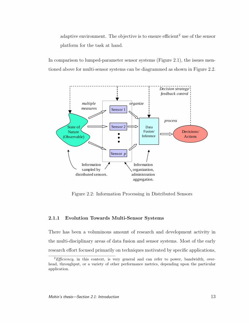
adaptive environment. The objective is to ensure efficient2 use of the sensor

platform for the task at hand.

In comparison to lumped-parameter sensor systems (Figure 2.1), the issues men-

tioned above for multi-sensor systems can be diagrammed as shown in Figure 2.2.

Sensor 1

Decisions/Actions

State ofNature

(Observable)

organize

process

Information sampled by

distributed sensors.

Information organization,

administration aggregation.

Decision strategy/feedback control

Sensor 2

Sensor p

DataFusion/

Inference

multiplemeasures

Figure 2.2: Information Processing in Distributed Sensors

2.1.1 Evolution Towards Multi-Sensor Systems

There has been a voluminous amount of research and development activity in

the multi-disciplinary areas of data fusion and sensor systems. Most of the early

research effort focused primarily on techniques motivated by specific applications,

2Efficiency, in this context, is very general and can refer to power, bandwidth, over-head, throughput, or a variety of other performance metrics, depending upon the particularapplication.


such as in vision systems, sonar, robotics platforms, etc. [47, 55, 62, 52]. Gradu-

ally, the inherent advantages of using multi-sensor systems were recognized [99, 6]

and a need for a comprehensive theory of the associated problems of distributed,

decentralized data fusion and multi-user information theory became apparent

[93, 28, 17]. A fundamental paradigm shift occurred with the maturing of inte-

grated circuit (IC) technologies in the last three decades. This allowed miniatur-

ized, low-cost sensors (among a whole host of other electronic devices) to be mass

produced and integrated with a wide variety of physical systems [24]. Parallel to

this development was the equally phenomenal revolution in wireless communica-

tion technologies. A concentrated amount of effort was directed towards solving

the general problems of wireless radio [48], and specific issues regarding wireless

ad hoc or peer-to-peer networking [32, 79, 86]. Subsequently, it was only natu-

ral to combine these two disciplines—sensors and networking—to develop a new

generation of distributed sensing devices that can work cooperatively to exploit

diversity. This has led to the birth of the Wireless Integrated Networked Sys-

tems (WINS) of sensors, among other ad hoc platforms [72, 73], and has fuelled

the associated research efforts over the last two decades in nano-technology and

micro-electro-mechanical (MEMS) systems [76].

Various researchers have attempted to develop practical systems that partly

address the aforementioned issues of efficient networking and data fusion for

sensors in the context of specific applications. However, the general problem

of efficient sensor administration for data fusion has not been comprehensively

addressed for heterogeneous sensors, possibly configured as an ad hoc or peer-to-

peer wireless network, in a mobile environment. In this thesis, in this and the

following chapters, these issues are addressed in an integrated framework, based

on information theoretic and system optimization principles. The objective is to

determine platform-independent guidelines and design philosophies that can be


used irrespective of the underlying application or hardware/software architecture.

Sensor Fusion Research:

For sensor technology in general, the key research thrust to date has been

in data fusion methodologies. As mentioned in Section 2.1, data fusion is the

process by which data from a multitude of sensor is used to yield an optimal

estimate of a specified state vector pertaining to the observed system [96], whereas

sensor administration is the design of communication and control mechanisms

for the efficient use of distributed sensors, with regards to power, performance,

reliability, etc. The main issues in sensor data fusion and sensor administration

have mostly been addressed separately, sometimes based on well-founded theories

and sometimes in an ad hoc manner and in the context of specific systems and

architectures. The research effort in sensor administration, in particular, has been

addressed primarily in the context of wireless networking, and not necessarily in

conjunction with the unique constraints imposed by data fusion methodologies.

To begin with, sensor models have been aimed at interpretation of measure-

ments. Such an approach to sensor modeling is exemplified in the models pre-

sented by Kuc and Siegel [47], among others. Probability theory, and in par-

ticular, a Bayesian treatment of data fusion emerged as a simple yet powerful

technique [96], and is arguably the most widely used method for describing un-

certainty in a way that abstracts from a sensor’s physical and operational de-

tails. Such quantitative methods have been used by researchers to evaluate and

model uncertainty in vision sensing, for example. Qualitative methods have also

been used to describe sensors, for example by Flynn [21] for sonar and infra-red

applications. Much work has also been done in developing methods for intel-

ligently combining information from different sensors. The basic approach has

been to pool the information using what are essentially ”weighted averaging”


techniques of varying degrees of complexity. For example Berger [6] discusses

a majority voting technique based on a probabilistic representation of informa-

tion. Non-probabilistic methods [29] used inferential techniques, for example for

multi-sensor target identification. Inferring the state of nature given a probabilis-

tic representation is, in general, a well understood problem in classical estima-

tion. Representative methods are Bayesian estimation, Least Squares estimation,

Kalman Filtering, and its various derivatives, etc. We anticipate that in systems

of the future, the question of what techniques to use for data aggregation will be

less pertinent than the question of how to use these techniques in a distributed

fashion, which has not been addressed to date in a systematic fashion, except for

some specific physical layer cases [97].

Sensor Administration Research:

In the area of sensor network administration, protocol development and man-

agement have mostly been addressed using application specific descriptive tech-

niques for specialized systems [99]. Much of the work has been in the area of

tracking radar systems, and robotics where the approach has been to develop

models of the sensor behavior and performance, and then manage the sensor

data transfer on that basis. This approach is facilitated by the centralized or

hierarchical nature of these systems (please see Section 2.4 for further discussions

on sensor network architectures). A large proportion of sensor allocation schemes

are based on determining cost functions and performance trade-offs a priori [5],

e.g. in using cost-benefit assignment matrices to allocate sensors to targets, or

using Boolean matrices which defines sensor-target assignments based on sensor

availability and capacity. Expert system approaches have also been used, as well

as normative or decision-theoretic techniques. However, optimal sensor admin-

istration in this way has been shown by Tsitsiklis [93] to be very hard in the


general framework of distributed sensors, and practical schemes use a mixture of

heuristic techniques (for example in data fusion systems involving wired sensors

in combat aircrafts). Only recently have the general networking issues for wire-

less ad hoc networks been addressed (Sohrabi, Singh [87, 83]), where the main

problems of self-organization, bootstrap, route discovery etc., have been identi-

fied. Application specific studies, e.g. in the context of antenna arrays (Yao,

[103]) have also discussed these issued. However, few general fusion rules or data

aggregation models for networked sensors have been proposed, with little analyt-

ical or quantitative emphasis. Most of these studies do not analyze in detail the

issues regarding the network-global impact of administration decisions, such as

choice of fusion nodes, path/tree selections, data fusion methodology, or physical

layer signalling details.

Fusion Architectures:

With regards to implementable sensor fusion architectures, current systems

are based on traditional centralized schemes, utilizing a central processor respon-

sible for implementing data fusion, or at best a hierarchical system for relieving

computation burdens at the central processor. But in the context of wireless sys-

tems, these schemes are not satisfactory because of the control and coordination

signaling overhead required. Also, these hierarchical architectures are vulnerable

to processor failure, computation bottlenecks and inflexibility. We believe that

to overcome these shortcomings, the recent trend towards autonomous systems

such as wireless sensor nodes (Pottie [73]) capable of creating an infrastructure

in an automated fashion is a feasible approach. These systems offer a number

of advantages: modularity by required the sensing and data fusion to take place

at the local nodes, at the lowest possible hierarchical level (which satisfies the

requirements of the various detection algorithms mentioned earlier); scalability


and flexibility, since the functionality is localized in the sensor and scaling the

system is simply a matter of designing robust network protocols for the admis-

sion and removal of additional sensor nodes; and survivability and fault tolerance,

due to the absence of a central processor, so the loss of nodes leads to a graceful

degradation in performance.

However, as yet, there is scant analysis of general (application-independent)

data fusion algorithms for such systems that operate in a wireless, distributed

configuration, with local and global fusion operations in parallel. This thesis

presents such an approach in the context of Information Processing, which can

be considered as an information-theoretic approach to sensor administration data

fusion.

2.1.2 An Information Processing Approach to Sensor Networks

It has been mentioned earlier that multi-sensor systems are basically information

gathering, analyzing and transmitting systems. The information being handled

almost always relates to a state of nature, and consequently, it is assumed to be

unknown prior to observation or estimation. Thus, the model of the information

flow shown in Figure 2.2 can be considered as a probabilistic model, and hence

can be quantified using the principles of Information Theory [14, 27]. Further-

more, the process of data detection and processing that occurs within the sensors

and fusion node(s) can be considered as elements of classical Statistical Decision

Theory [70]. Using the mature techniques that these disciplines offer, a proba-

bilistic information processing relation can then be quantified for sensor networks,

and analyzed within the framework of the well-known Bayesian Paradigm [78].

Using this approach, this thesis presents a unified treatment of probabilistic in-

formation processing as they relate to the issues of data representation, fusion,


and transmission in decentralized sensor networks.

In particular, for the administration of multi-sensor systems, the autonomous

nature of individual sensor nodes and the presence or absence of a central pro-

cessor raises problems such as:

• consistency and consensus among decision-makers

• group vs. individual optimality for decisions

• data and network synchronization for coherent processing of information

• physical layer issues.

It is shown in this thesis that the core elements of these problems can be quan-

titatively formulated and analyzed using the information processing framework

mentioned above. Performance issues can then be studied theoretically, and

system level optimizations can be carried out efficiently. References to the

appropriate sections in the chapters here....

Using this approach, this thesis sub-divides the issues into the following sub-

problems.

1. Determination of appropriate information processing techniques, models

and metrics for fusion and sensor administration.

2. Representation of the sensors process, data fusion, and administration me-

thodologies using the appropriate probabilistic models.

3. Analysis of the measurable aspects of the information flow in the sensor

architecture using the defined models and metrics.

4. Design of optimum data fusion algorithms and architectures for optimum

inference in multi-sensor systems.


5. Design, implementation and test of associated networking and physical layer

algorithms and architectures for the models determined in (4).

The subsequent sections in this thesis address these issues, beginning with a

Bayesian scheme for generalizing the data fusion problem.

2.2 A Bayesian Scheme for Decentralized Data Fusion

Sensors provide an estimate of nature, and thus can be viewed as sources of infor-

mation. In a multi-sensor system, several such information sources are available,

so it is possible to implement different strategies for combining the information

from multiple sources. Two issues are of immediate interest: (i) the nature of

the information being generated the sensors, and (ii) the method of combining

the information from disparate sources. We consider the first issue first.

2.2.1 Sensor Data Model for Single Sensors

It is a fact of nature that any observation or measurement by any sensor is

always uncertain to a degree determined by the precision of the sensor. This

uncertainty, or measurement noise, requires us to treat the data generated by

a sensor probabilistically. We therefore adopt the notation and definitions of

probability theory to determine an appropriate model for sensor data [25].

Definiton 2.1. A state vector at time instant t, is a representation of the state

of nature of a process of interest, and can be expressed as a vector x(t) in a

measurable, finite-dimensional vector space, Ω, over a discrete or continuous field,

F:

Mohin’s thesis—Section 2.2: A Bayesian Scheme for Decentralized

Data Fusion 20

x(t) =

x1

x2

...

xn

∈ Ω (2.1)

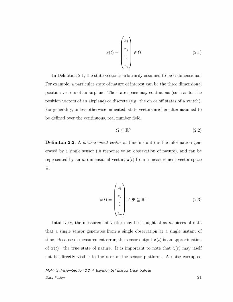
In Definition 2.1, the state vector is arbitrarily assumed to be n-dimensional.

For example, a particular state of nature of interest can be the three dimensional

position vectors of an airplane. The state space may continuous (such as for the

position vectors of an airplane) or discrete (e.g. the on or off states of a switch).

For generality, unless otherwise indicated, state vectors are hereafter assumed to

be defined over the continuous, real number field.

Ω ⊆ Rn (2.2)

Definiton 2.2. A measurement vector at time instant t is the information gen-

erated by a single sensor (in response to an observation of nature), and can be

represented by an m-dimensional vector, z(t) from a measurement vector space

Ψ.

z(t) =

z1

z2

...

zm

∈ Ψ ⊆ Rm (2.3)

Intuitively, the measurement vector may be thought of as m pieces of data

that a single sensor generates from a single observation at a single instant of

time. Because of measurement error, the sensor output z(t) is an approximation

of x(t)—the true state of nature. It is important to note that z(t) may itself

not be directly visible to the user of the sensor platform. A noise corrupted


Data Fusion 21

version Γz(t),v(t), as defined below, may be all that is available for processing.

Furthermore, the dimensionality of the sensor data may not be the same as

the dimension of the observed parameter that is being measured. For example,

continuing with the airplane example, a sensor may display the longitude and

latitude of the airplane at a particular instant of time via GPS (a 2-dimensional

observation vector), but may not be able to measure the altitude of the airplane

(which completes the 3-dimensional specification of the actual location of the

airplane in space).

The measurement error itself can be considered as another vector, v(t), or a

noise process vector, of the same dimensionality as the observation vector z(t).

As the name suggests, noise vectors are inherently stochastic in nature, and serve

to render all sensor measurements uncertain, to a specific degree.

Definiton 2.3. An observation model, Γ, for a sensor is a mapping from state

space Ω to observation space Ψ, and is parameterized by the statistics of the

noise process:

Γv : Ω 7→ Ψ. (2.4)

Functionally, the relationship between the state, observation and noise vectors

can be expressed as:

z(t) = Γ x(t), v(t) . (2.5)

Objective: The objective in sensing applications is to infer the unknown state

vector x(t) from the error corrupted and (possibly lower dimensional) observation

vector z(t),v(t). If the functional specification of the mapping in Equation (2.4),

and the noise vector v(t), were known for all times t, then finding the inverse

mapping for one-to-one cases would be trivial, and the objective would be easily

achieved. It is precisely because either or both parameters may be random that

gives rise to various estimation architectures for inferring the state vector from


Data Fusion 22

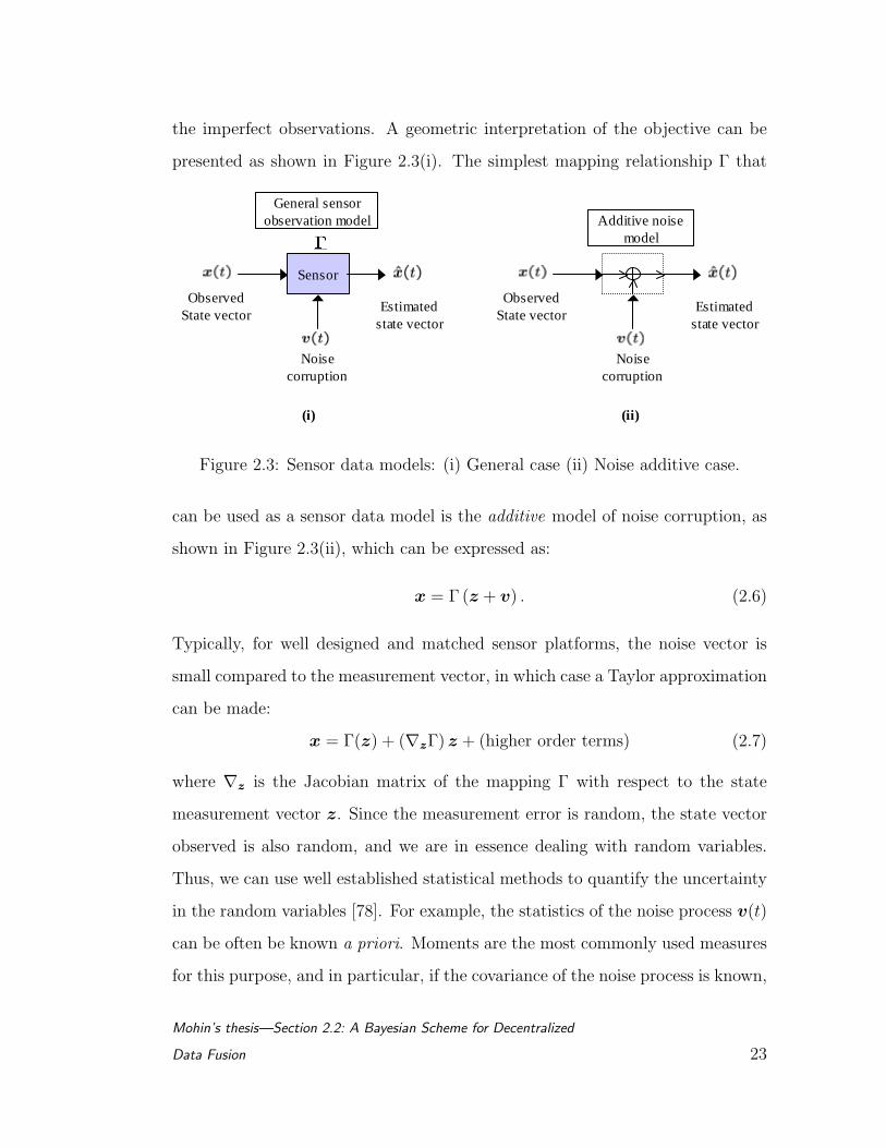
the imperfect observations. A geometric interpretation of the objective can be

presented as shown in Figure 2.3(i). The simplest mapping relationship Γ that

Sensor

Observed State vector

Estimated state vector

Noise corruption

General sensorobservation model

(i)

Observed State vector

Estimated state vector

Noise corruption

Additive noise model

(ii)

Figure 2.3: Sensor data models: (i) General case (ii) Noise additive case.

can be used as a sensor data model is the additive model of noise corruption, as

shown in Figure 2.3(ii), which can be expressed as:

x = Γ (z + v) . (2.6)

Typically, for well designed and matched sensor platforms, the noise vector is

small compared to the measurement vector, in which case a Taylor approximation

can be made:

x = Γ(z) + (∇zΓ) z + (higher order terms) (2.7)

where ∇z is the Jacobian matrix of the mapping Γ with respect to the state

measurement vector z. Since the measurement error is random, the state vector

observed is also random, and we are in essence dealing with random variables.

Thus, we can use well established statistical methods to quantify the uncertainty

in the random variables [78]. For example, the statistics of the noise process v(t)

can be often be known a priori. Moments are the most commonly used measures

for this purpose, and in particular, if the covariance of the noise process is known,


Data Fusion 23

EvvT

, then the covariance of the state vector can be expressed as:

ExxT

= (∇zΓ)E

vvT

(∇zΓ)T . (2.8)

For uncorrelated noise v, the matrix (∇zΓ)EvvT

(∇zΓ)T is symmetric and

can be decomposed using singular value decomposition [80]:

(∇zΓ) EvvT

(∇zΓ)T =

(SDST

)(2.9)

where S is an (n× n) matrix of orthogonal vectors ej and D are the eigenvalues

of the decomposition:

S = (e1, e2, · · · , en) , eiej =

1 for i = j

0 for i 6= j(2.10)

D = diag (d1, d2, . . . , dn) (2.11)

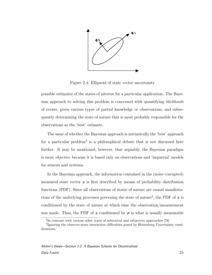
The scalar variance in each direction corresponding to each of the components

of x is given by the corresponding component of D. When all the directions

are considered for a given state x, the geometrical result is an ellipsoid in n-

dimensional space, with the principal axes in the directions of the vectors ek

and 2√

dj as the corresponding magnitudes. The volume of the ellipsoid is the

uncertainty in x. The 2-dimensional case is shown in Figure 2.4. Therefore, in

a geometric sense, the aim is to reduce the volume of the uncertainty ellipsoid.

All the techniques for data estimation, fusion, and inference are designed towards

this goal [63].

The most celebrated method among them is the probabilistic method derived

from Bayes’ Law [25].

2.2.2 Bayesian Estimation and Inference

Given the inherent uncertainty in measurements of states of nature, the end

goal in using sensors, as mentioned in the previous section, is to obtain the best


Data Fusion 24

e 1

e 2

e 1

e 2

Figure 2.4: Ellipsoid of state vector uncertainty

possible estimates of the states of interest for a particular application. The Baye-

sian approach to solving this problem is concerned with quantifying likelihoods

of events, given various types of partial knowledge or observations, and subse-

quently determining the state of nature that is most probably responsible for the

observations as the ‘best’ estimate.

The issue of whether the Bayesian approach is intrinsically the ‘best’ approach

for a particular problem3 is a philosophical debate that is not discussed here

further. It may be mentioned, however, that arguably, the Bayesian paradigm

is most objective because it is based only on observations and ‘impartial’ models

for sensors and systems.

In the Bayesian approach, the information contained in the (noise corrupted)

measured state vector z is first described by means of probability distribution

functions (PDF). Since all observations of states of nature are causal manifesta-

tions of the underlying processes governing the state of nature4, the PDF of z is

conditioned by the state of nature at which time the observation/measurement

was made. Thus, the PDF of z conditioned by x is what is usually measurable

3In contrast with various other types of inferential and subjective approaches [78]4Ignoring the observer-state interaction difficulties posed by Heisenberg Uncertainty consi-

derations.


Data Fusion 25

and is represented by:

FZ(z | x) (2.12)

This is known as the Likelihood Function for the observation vector. Next, if

information about the possible states under observation is available (e.g. a pri-

ori knowledge of the range of possible states), or more precisely the probability

distribution of the possible states FX(x), then the prior information and the like-

lihood function (2.12) can be combined to provide the a posteriori conditional

distribution of x, given z, by the famous Bayes’ Theorem:

Theorem 2.1.

FX(x | z) =FZ(z | x)FX(x)∫

Ω

FZ(z | x)FX(x) dF (x)=

FZ(z | x)FX(x)

FZ(z)(2.13)

Usually, some function of the actual likelihood function, g(T (z) | x), is com-

monly available as the processable information from sensors. T (z) is known as

the sufficient statistic for x and Equation (2.13) can be reformulated as:

FX(x | z) = FX(x | T (z)) =g(T (z) | x)FX(x)∫

Ω

g(T (z) | x)FX(x) dF (x)

(2.14)

If the observations are assumed to be carried out in discrete time steps, according

to a desired resolution, then a vector version of the above-mentioned formulation

can be derived. Defining all observations upto time index r as:

Zr , z(1),z(2), . . . , z(r) (2.15)

then the posterior distribution of x given the set of observations vecZr is:

FX(x | Zr) =FZr(Zr | x)FX(x)

FZr(Zr)(2.16)


Data Fusion 26

Using the same idea, a recursive version of Equation (2.16) can also be formulated

as follows:

FX(x | Zr) =FZ(z(r) | x)FX(x | Zr−1)

FZ(z(r) | Zr−1)(2.17)

in which case all the r observations do not need to be stored, and instead only the

current observation z(r) can be considered at the rth step. This version of the

Bayes’ Law is most prevalent in practice since it offers a directly implementable

technique for fusing observed information with prior beliefs.

2.2.3 Classical Estimation Techniques

In Section 2.2.2, a likelihood function framework was developed for the measured

state vectors from sensors. Given this framework, a variety of inference techniques

can now be applied to estimate the state vector x (from the time series obser-

vations from a single sensor). Note that the estimate, denoted by x, is derived

from the posterior distribution Fvecx(x | Zr) and is a point in the uncertainty

ellipsoid of Figure 2.4. The objective of all the estimation techniques outlined

in this section is to reduce the volume of the ellipsoid, which is equivalent to

minimizing the probability of error based on some criterion. Three classical tech-

niques are now briefly reviewed: Maximum Likelihood, Maximum A Posteriori

and Minimum Mean Square Error estimation.

Maximum Likelihood (ML) estimation involves maximizing the likelihood func-

tion (Equation 2.12) by some form of search over the state space Ω:

xML = arg maxx∈Ω

FZr (Zr | x) (2.18)

This is intuitive since the PDF is greatest when the correct state has been guessed

for the conditioning variable. However, a major drawback of this technique is

that for state vectors from large state spaces, the search may be computationally


Data Fusion 27

expensive, or infeasible. Despite this shortcoming, this method is widely used in

many disciplines, and is prominent for wireless digital reception techniques [74].

Maximum a posteriori (MAP) estimation technique involves maximizing the

posterior distribution from observed data as well as from prior knowledge of the

state space:

xMAP = arg maxx∈Ω

Fx (x | Zr) (2.19)

Since prior information may be subjective, objectivity for an estimate (or the

inferred state) is maintained by considering only the likelihoood function (i.e. only

the observed information). In the instance of no prior knowledge, and the state

space vectors are all considered to equally likely, the MAP and ML criterion can

be shown to be identical.

Minimum Mean Square Error (MMSE) estimation is an estimation technique

that attempts to minimize the estimation error by searching over the state space,

albeit in an organized fashion. This is the most popular technique in a wide vari-

ety of information processing applications, since the variable can often be found

analytically, or the search space can be reduced considerably or investigated sys-

tematically. The key notion is to reduce the covariance of the estimate. Defining

the mean and variance of the posterior observation variable as:

x , EF (x|Zr)x (2.20)

Var(x) , EF (x|Zr)(x − x)(x − x)T (2.21)

it can be shown that the least squares estimator is one that minimizes the Eu-

clidean distance between the true state x and the estimate x, given the set of

observations Zr. In the context of random variables, this estimator is referred to

as the MMSE estimate and can be expressed as:

xMMSE = arg minx∈Ω

EF (x|Zr)(x − x)(x − x)T (2.22)


Data Fusion 28

To obtain the minimizing estimate, Equation (2.22) can be differentiated with

respect to x and set equal to zero, which yields:

∇x∫

x∈Ω

(x − x)T (x − x)F (x | Zr) dF (x)

= −2

∫

x∈Ω

(x − x)F (x | Zr) dF (x) = 0

from where x = E x | Zr(2.23)

Thus the MMSE estimate is the conditional mean. It also can be shown that

the MMSE estimate is the minimum variance estimate, and when the conditional

density coincides with the mode, the MAP and MMSE estimators are equivalent.

These estimation techniques and their derivatives such as the Wiener and

Kalman filters [42] all serve to reduce the uncertainty ellipsoid associated with

state x [63], which was the stated objective of this section.

As mentioned at the outset in Section 2.2.1, all the techniques presented

thus far are applicable only to the case of a single sensor, where multiple time-

step observations are used to reduce uncertainty. When multiple, distributed

sensors are involved, in a variety of configurations and topologies, some additional

machinery is required to be able to combine the information from these disparate

sources. This is developed in the next section.

2.2.4 Sensor Data Model for Multi-Sensor Systems

When a number of spatially and functionally different sensor systems are used to

observe the same (or similar) state of nature, then the data fusion problem is no

longer simply a state space uncertainty minimization issue. The distributed and

multi-dimensional nature of the problem requires a technique for checking the


Data Fusion 29

usefulness and validity of the data from each of the not necessarily independent

sensors. The data fusion problem is more complex, and general solutions are not

readily evident. This section explores some of the commonly studied techniques

and proposes a novel, simplified methodology that achieves some measure of

generality.

The first issue is, once again, the proper modeling of the data sources. The

nomenclature and technique introduced in Section 2.2.1 can be extended to mul-

tiple sensors. If there are p sensors observing the same state vector, but from

different vantage points, and each one generates its own observations, then we

have a collection of observation vectors z1(t), z2(t), . . . , zp(t), which can be rep-

resented as a combined matrix of all the observations from all sensors (at any

particular time t):

Z(t) =(z1(t) z2(t) · · · zp(t)

)=

z11 z21 · · · zp1

z12 z22 · · · zp2

. . .

z1m z2m · · · zpm

. (2.24)

Furthermore, if each sensor makes observations upto time step r for a dis-

cretized (sampled) observation scheme, then the matrix of observations Z)(r)

can be used to represent the observations of all the p sensors at time-step r (a

discrete variable, rather than the continuous Z(t)). If memory is allowed for the

signal processing of these data, then we can consider the super-matrix Zr of

all the observations of all the p sensors from time step 0 to time step r:

Zr =

p⋃i=1

Zri (2.25)

where Zri = zi(1),zi(2), . . . zi(r) (2.26)

This suggests that to use all the available information for effectively fusing the


Data Fusion 30

data from multiple sensors, what is required is the global posterior distribution

Fx (x | Zr), given the time-series information from each source. This can be

accomplished in a variety of ways, the most common of which are summarized

below.

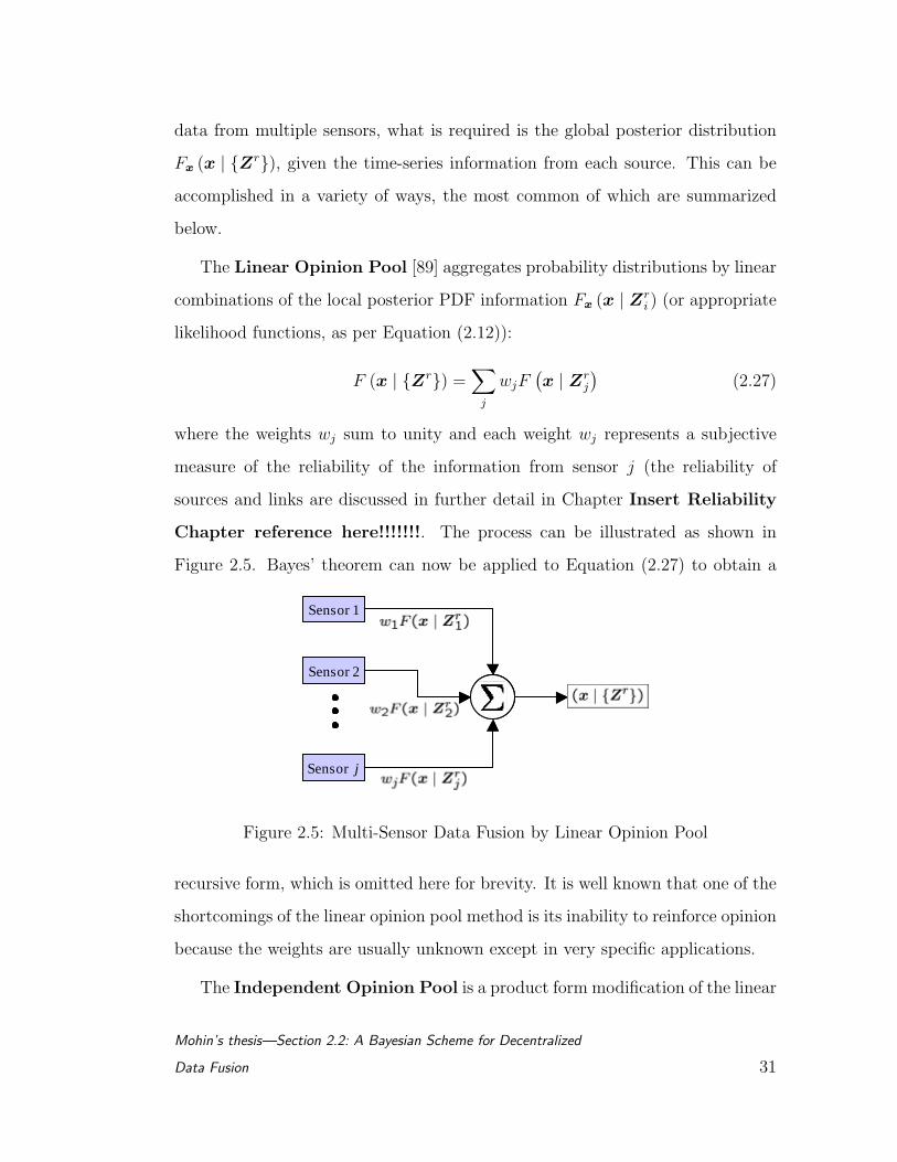
The Linear Opinion Pool [89] aggregates probability distributions by linear

combinations of the local posterior PDF information Fx (x | Zri ) (or appropriate

likelihood functions, as per Equation (2.12)):

F (x | Zr) =∑

j

wjF(x | Zr

j

)(2.27)

where the weights wj sum to unity and each weight wj represents a subjective

measure of the reliability of the information from sensor j (the reliability of

sources and links are discussed in further detail in Chapter Insert Reliability

Chapter reference here!!!!!!!. The process can be illustrated as shown in

Figure 2.5. Bayes’ theorem can now be applied to Equation (2.27) to obtain a

Sensor 1

Sensor 2

Sensor j

Sensor 1

Sensor 2

Sensor j

Figure 2.5: Multi-Sensor Data Fusion by Linear Opinion Pool

recursive form, which is omitted here for brevity. It is well known that one of the

shortcomings of the linear opinion pool method is its inability to reinforce opinion

because the weights are usually unknown except in very specific applications.

The Independent Opinion Pool is a product form modification of the linear


Data Fusion 31

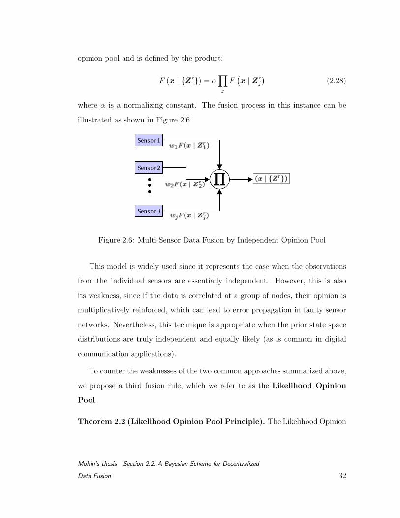
opinion pool and is defined by the product:

F (x | Zr) = α∏

j

F(x | Zr

j

)(2.28)

where α is a normalizing constant. The fusion process in this instance can be

illustrated as shown in Figure 2.6

Sensor 1

Sensor 2

Sensor j

Figure 2.6: Multi-Sensor Data Fusion by Independent Opinion Pool

This model is widely used since it represents the case when the observations

from the individual sensors are essentially independent. However, this is also

its weakness, since if the data is correlated at a group of nodes, their opinion is

multiplicatively reinforced, which can lead to error propagation in faulty sensor

networks. Nevertheless, this technique is appropriate when the prior state space

distributions are truly independent and equally likely (as is common in digital

communication applications).

To counter the weaknesses of the two common approaches summarized above,

we propose a third fusion rule, which we refer to as the Likelihood Opinion

Pool.

Theorem 2.2 (Likelihood Opinion Pool Principle). The Likelihood Opinion


Data Fusion 32

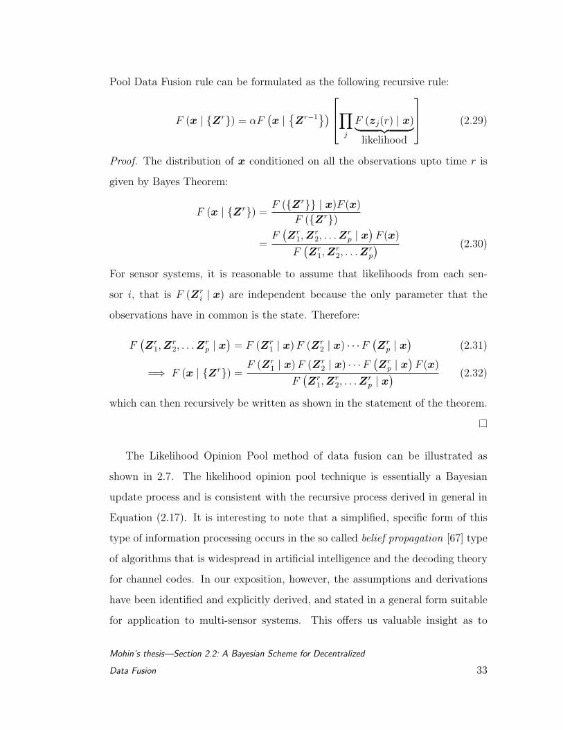
Pool Data Fusion rule can be formulated as the following recursive rule:

F (x | Zr) = αF(x | Zr−1

)

∏j

F (zj(r) | x)︸︷︷︸likelihood

(2.29)

Proof. The distribution of x conditioned on all the observations upto time r is

given by Bayes Theorem:

F (x | Zr) =F (Zr | x)F (x)

F (Zr)

=F

(Zr

1, Zr2, . . . Z

rp | x

)F (x)

F(Zr

1,Zr2, . . . Z

rp

) (2.30)

For sensor systems, it is reasonable to assume that likelihoods from each sen-

sor i, that is F (Zri | x) are independent because the only parameter that the

observations have in common is the state. Therefore:

F(Zr

1,Zr2, . . . Z

rp | x

)= F (Zr

1 | x) F (Zr2 | x) · · ·F (

Zrp | x

)(2.31)

=⇒ F (x | Zr) =F (Zr

1 | x) F (Zr2 | x) · · ·F (

Zrp | x

)F (x)

F(Zr

1,Zr2, . . . Z

rp | x

) (2.32)

which can then recursively be written as shown in the statement of the theorem.

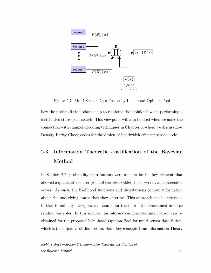
The Likelihood Opinion Pool method of data fusion can be illustrated as

shown in 2.7. The likelihood opinion pool technique is essentially a Bayesian

update process and is consistent with the recursive process derived in general in

Equation (2.17). It is interesting to note that a simplified, specific form of this

type of information processing occurs in the so called belief propagation [67] type

of algorithms that is widespread in artificial intelligence and the decoding theory

for channel codes. In our exposition, however, the assumptions and derivations

have been identified and explicitly derived, and stated in a general form suitable

for application to multi-sensor systems. This offers us valuable insight as to


Data Fusion 33

Sensor 1

Sensor 2

Sensor j

a priori informat ion

Figure 2.7: Multi-Sensor Data Fusion by Likelihood Opinion Pool

how the probabilistic updates help to reinforce the ‘opinions’ when performing a

distributed state space search. This viewpoint will also be used when we make the

connection with channel decoding techniques in Chapter 6, where we discuss Low

Density Parity Check codes for the design of bandwidth efficient sensor nodes.

2.3 Information Theoretic Justification of the Bayesian

Method

In Section 2.2, probability distributions were seen to be the key element that

allowed a quantitative description of the observables, the observer, and associated

errors. As such, the likelihood functions and distributions contain information

about the underlying states that they describe. This approach can be extended

further to actually incorporate measures for the information contained in these

random variables. In this manner, an information theoretic justification can be

obtained for the proposed Likelihood Opinion Pool for multi-sensor data fusion,

which is the objective of this section. Some key concepts from Information Theory

Mohin’s thesis—Section 2.3: Information Theoretic Justification of

the Bayesian Method 34

are required first.

2.3.1 Information Measures

Information theory was developed to determine the fundamental limits on the

performance of communication systems [81]. Detection theory on the other hand,

as we have seen, involves the application of statistical decision theory to estimate

states of nature. Both these disciplines can be used to treat problems in the

transmission and reception of information. This synergy was first explored by

researchers in the 1950s and 1960s [60], and the well established source and

channel coding theories have spawned as a result.

A similar approach can be taken to leverage the fundamental concepts of

these disciplines for multi-sensor data fusion and distributed detection problems.

This has been studied since the 1970s and 1980s [96], and a brief survey was

provided in Section 2.1.1. In Section 2.2, we also presented the Bayesian approach

which we believe is the most straightforward application of the key results from

detection theory for accomplishing distributed data-fusion. In this section, an

information theoretic justification is provided as to the utility of the Bayesian

update method. It also serves to provide insight towards the practical design of

algorithms based on the proposed likelihood opinion pool fusion rules, which are

discussed in Section 2.4.

To build an information theoretic foundation for data fusion, the most useful

fundamental metric is the Shannon definition of Entropy.

Definiton 2.4. Entropy is the uncertainty associated with a probability distri-

bution, and is a measure of the descriptive complexity of a PDF [11]. Mathemat-

ically:

hF (x) , E− ln F (x) (2.33)



Note that alternative definitions of the concept of information which predate

Shannon’s formulation, e.g. the Fisher Information Matrix [20], are also relevant

and useful, but not discussed here further.

Using this definition, an expression for the entropy of the posterior distribution

of x given Zr at time r (which is the case of multiple observations from a single

sensor) can be expressed as:

h(r) , h F (x | Zr) = −∑

F (x | Zr)lnF (x | Zr) (2.34)

From this definition, the entropy relationship for Bayes Theorem can be developed

as follows:

E − ln[F (x | Zr)] = E− ln[F (x | Zr−1)]

− E

ln

[F (z(r) | x)

F (z(r) | Zr−1)

](2.35)

=⇒ h(r) = h(r − 1)− E

ln

[F (z(r) | x)

F (z(r) | Zr−1)

](2.36)

This is an alternative form of the result that conditioning with respect to ob-

servations reduces entropy (cf. [14]). Using the definition of mutual information,

Equation (2.35) can be written in an alternative form as shown below.

Definiton 2.5. For an observation process, mutual information at time r is the

information about x contained in the observation z(r):

I(x, z(r)) , E

ln

[F (z(r) | x)

F (z(r))

](2.37)

from where

h(r) = h(r − 1)− I(r) (2.38)

which means that the entropy following an observation is reduced by an amount

equal to the information inherent in the observation.



The insight to be gained here is that by using the above mentioned defini-

tions of entropy and mutual information, the recursive Bayes update procedure

derived in Section 2.2.2 Equation (2.17) can now be seen as an information update

procedure:

E ln[F (x | Zr)] = Eln[F (x | Zr−1)]

+ E

ln

[F (z(r) | x)

F (z(r) | Zr−1)

](2.39)

which can be interpreted as:

posterior information = prior information + observation information.

The information update equations can then be written for the proposed Like-

lihood Opinion Pool fusion rule, which becomes:

E ln[F (x | Zr)] = Eln[F (x | Zr−1)]

+∑

j

E

ln

[F (zj(r) | x)

F (zj(r) | Zr−1)

](2.40)

The utility of the log-likelihood definition is in the fact that the information

update steps then reduce to simple additions, and are thus amenable to hardware

implementation without problems of overflow, dynamic range scaling, etc.

This section has thus shown that the Bayesian probabilistic approach is theo-

retically self-sufficient for providing a unified framework for data fusion in multi-

sensor platforms. The information theoretic connection to the Bayesian update

makes the approach intuitive, and shows rigorously how the proposed Likelihood

Opinion Pool method serves to reduce the ellipsoid uncertainty.

In the following sections, these theoretical developments are used to design and

determine the actual architectures that can be used for data fusion in practical

multi-sensor systems.



2.4 Multi-Sensor Data Fusion Architectures

The information processing approach of 2.2 allows us to reduce the problem of

data fusion, regardless of the application, network or physical layer design, to one

of information fusion. This, as we have seen, is basically a Bayesian update of

likelihoods. Thus, the problem of designing an appropriate architecture for data

fusion can be decoupled from system-specific concerns. This is a major advantage.

The general results derived in the previous sections can now be used to determine

appropriate platform independent data fusion architectures for distributed sensor

networks.

Some versions of this concept were recognized early in the robotics and vi-

sion systems community [63, 21]. In the following sections, the architectures are

classified and a novel scheme based on the Likelihood Opinion Pool formulation

is provided.

2.4.1 Classification of Sensor Network Architectures

The information processing approach can be used to design three distinct types

of sensor data fusion network architectures.

1. Centralized Architecture

2. Hierarchical Architecture

3. Distributed Architecture (fully and non-fully connected)

We provide the general definitions of each of these types of architectures in the

following paragraphs, borrowing terminology from graph theory [100].

Definiton 2.6. A Centralized Architecture for multi-sensor data fusion is a star

network topological arrangement of sensor nodes, with a central processor at the

Mohin’s thesis—Section 2.4: Multi-Sensor Data Fusion Architectures 38

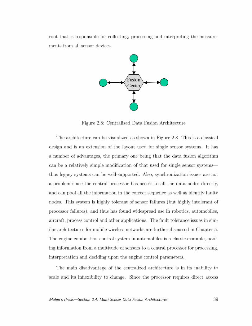
root that is responsible for collecting, processing and interpreting the measure-

ments from all sensor devices.

FusionCenter

Figure 2.8: Centralized Data Fusion Architecture

The architecture can be visualized as shown in Figure 2.8. This is a classical

design and is an extension of the layout used for single sensor systems. It has

a number of advantages, the primary one being that the data fusion algorithm

can be a relatively simple modification of that used for single sensor systems—

thus legacy systems can be well-supported. Also, synchronization issues are not

a problem since the central processor has access to all the data nodes directly,

and can pool all the information in the correct sequence as well as identify faulty

nodes. This system is highly tolerant of sensor failures (but highly intolerant of

processor failures), and thus has found widespread use in robotics, automobiles,

aircraft, process control and other applications. The fault tolerance issues in sim-

ilar architectures for mobile wireless networks are further discussed in Chapter 5.

The engine combustion control system in automobiles is a classic example, pool-

ing information from a multitude of sensors to a central processor for processing,

interpretation and deciding upon the engine control parameters.

The main disadvantage of the centralized architecture is in its inability to

scale and its inflexibility to change. Since the processor requires direct access


to each of the sensors, the system is unmanageable for large numbers of sensors.

The computational burden on the processor grows exponentially. In a wired

application, the problems of physically connecting the nodes to the processor also

rules out its use for distributed applications. In mobile wireless scenarios, direct

single-hop links from the fusion center to all distributed nodes are hardly always

feasible, and the overhead and QoS issues involved in establishing and maintaining

the required star-network with the processor as the root can be overwhelming.

Finally, processor fault (in)tolerance is a catastrophic shortcoming. Any failures

of the central processor renders the architecture useless. To counter this defect,

mission critical systems often have double and triple redundancy modes [50],

e.g. the guidance system in the Space Shuttle. However, redundancy may not be

cost effective or manageable in applications requiring mass scenarios.

To counter some of the disadvantages of centralized architectures, hierarchical

fusion arrangements have been devised.

Definiton 2.7. A Hierarchical Architecture for multi-sensor data fusion is a tree

network topological arrangement of sensors and processors. The tree is rooted

at the global fusion center, and the sensors occupy the leaves of the tree, and

intermediate nodes serve as the local fusion processors.

A hierarchical arrangement can be illustrated as shown in Figure 2.9. In such

schemes, local fusion processors handle the data from a subset of the sensors, and

a global fusion center then pools the information from the local fusion sources for

processing and inference. The global fusion center serves to relieve the computa-

tional burden on each of the local processors by a divide and conquer strategy.

The primary advantage of the hierarchical system is in its ability to incor-

porate different classes of sensors as part of different local groups. Hence, het-

erogeneous types of networked sensor systems can be supported in this scheme.


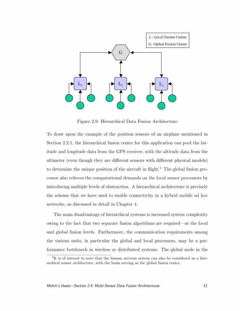
G

L : Local Fusion Center

G: Global Fusion Center

L1L1 L1L1 L1L1

Figure 2.9: Hierarchical Data Fusion Architecture

To draw upon the example of the position sensors of an airplane mentioned in

Section 2.2.1, the hierarchical fusion center for this application can pool the lat-

itude and longitude data from the GPS receiver, with the altitude data from the

altimeter (even though they are different sensors with different physical models)

to determine the unique position of the aircraft in flight.5 The global fusion pro-

cessor also relieves the computational demands on the local sensor processors by

introducing multiple levels of abstraction. A hierarchical architecture is precisely

the scheme that we have used to enable connectivity in a hybrid mobile ad hoc

networks, as discussed in detail in Chapter 4.

The main disadvantage of hierarchical systems is increased system complexity

owing to the fact that two separate fusion algorithms are required—at the local

and global fusion levels. Furthermore, the communication requirements among

the various units, in particular the global and local processors, may be a per-

formance bottleneck in wireless or distributed systems. The global node in the

5It is of interest to note that the human nervous system can also be considered as a hier-archical sensor architecture, with the brain serving as the global fusion center.


hierarchy also inherits the vulnerability to failures as in the centralized architec-

ture case. However, it is of interest to note that the global fusion process may

itself reside on one (or more) of the local fusion centers. This enables a form of

processor redundancy fault tolerance. In case the global fusion center fails, and

one of the other surviving local fusion centers can function as a global center,

then fusion control can pass to this new global fusion center. There are issues

regarding handshaking and leader election under such circumstances. However,

these are manageable, and the scheme has been implemented in the context of

gateways in hybrid mobile ad hoc networks of processors (Chapter 4).

For maximum flexibility, a decentralized system for multi-sensor data fusion

offers the best means of overcoming the problems associated with both centralized

and hierarchical architectures.

Definiton 2.8. A Decentralized Architecture for multi-sensor data fusion is an

ad hoc network topology of sensors nodes and data fusion processors, with at

least one connected component consisting of sensors and processors.

A decentralized architecture is an example of an arbitrary ad hoc network of

nodes (Section 4.2). However, for the case of sensor networks, it is of interest to

have at least one connected component of sensors and processors, because, with-

out communication between these elements, there can be no fusion process pos-

sible. Thus, one extreme case of a decentralized architecture is a fully connected

graph of sensor and processor nodes, and the other extreme is an arbitrarily

connected network of sensor and processor nodes (Figure 2.10).

Decentralized architectures do not rely on any specific sensor, or fusion pro-

cessor (which may be the same physical device), for its operations. Therefore,

any fault or failure of any subset of the nodes do not cause a catastrophic failure

of the system. This has very desirable fault tolerance properties. Furthermore,


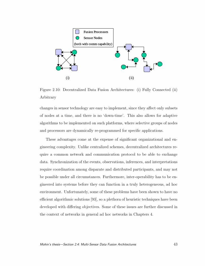
Fusion Processors

Sensor Nodes

(both with comm capability)

Fusion Processors

Sensor Nodes

(both with comm capability)

(i) (ii)

Figure 2.10: Decentralized Data Fusion Architectures: (i) Fully Connected (ii)

Arbitrary

changes in sensor technology are easy to implement, since they affect only subsets

of nodes at a time, and there is no ‘down-time’. This also allows for adaptive

algorithms to be implemented on such platforms, where selective groups of nodes

and processors are dynamically re-programmed for specific applications.

These advantages come at the expense of significant organizational and en-

gineering complexity. Unlike centralized schemes, decentralized architectures re-

quire a common network and communication protocol to be able to exchange

data. Synchronization of the events, observations, inferences, and interpretations

require coordination among disparate and distributed participants, and may not

be possible under all circumstances. Furthermore, inter-operability has to be en-

gineered into systems before they can function in a truly heterogeneous, ad hoc

environment. Unfortunately, some of these problems have been shown to have no

efficient algorithmic solutions [93], so a plethora of heuristic techniques have been

developed with differing objectives. Some of these issues are further discussed in

the context of networks in general ad hoc networks in Chapters 4.


2.4.2 An Architecture for Likelihood Opinion Pool Data Fusion

In this section, the architectural concepts outlined in Section 2.4.1 are extended

to introduce a generalized form of a distributed multi-sensor data fusion archi-

tecture, based on the Likelihood Opinion Pool formulation.

To begin with, a choice needs to be made at the outset regarding the basic

type of information that will be transmitted in a multi-sensor system. For ex-

ample, upon observation and measurement of a state of nature, a sensor may

transmit either the raw data z(r) at each time step r, or the likelihood infor-

mation [αiF (zi(r) | x)], or the sufficient statistics formulations F (Tzi(r) | x)

(Section 2.2.4). However, the communication of raw sensor data requires the

central processor to have knowledge of the models for each sensor so that the

likelihoods can be computed from the observations from all the sensors. This is

an inflexible option. Instead, as we have seen from Section 2.3.1, the likelihood

contains essentially the same information, but in a much more convenient form,

since then the sensor model can be kept locally at each sensor and only ‘soft’ met-

rics can be sent to a general fusion processor. From a systems implementation

and computation point of view, this is an attractive choice. Sufficient statistics

metrics are essentially similar, the only difference being a data space transforma-

tion; the fusion processor still does not need to maintain a sensor profile for each

sensor in the network.

With likelihoods being the currency, as it were, being traded in the sensor

network, we note that in the Bayesian information processing formulation (Sec-

tion 2.3), the update at time step r for a single sensor can be written in terms of

the log-likelihood as:

ln F (x | Zr) = ln F (x | Zr−1) + ln[αF (z(k) | x)] (2.41)


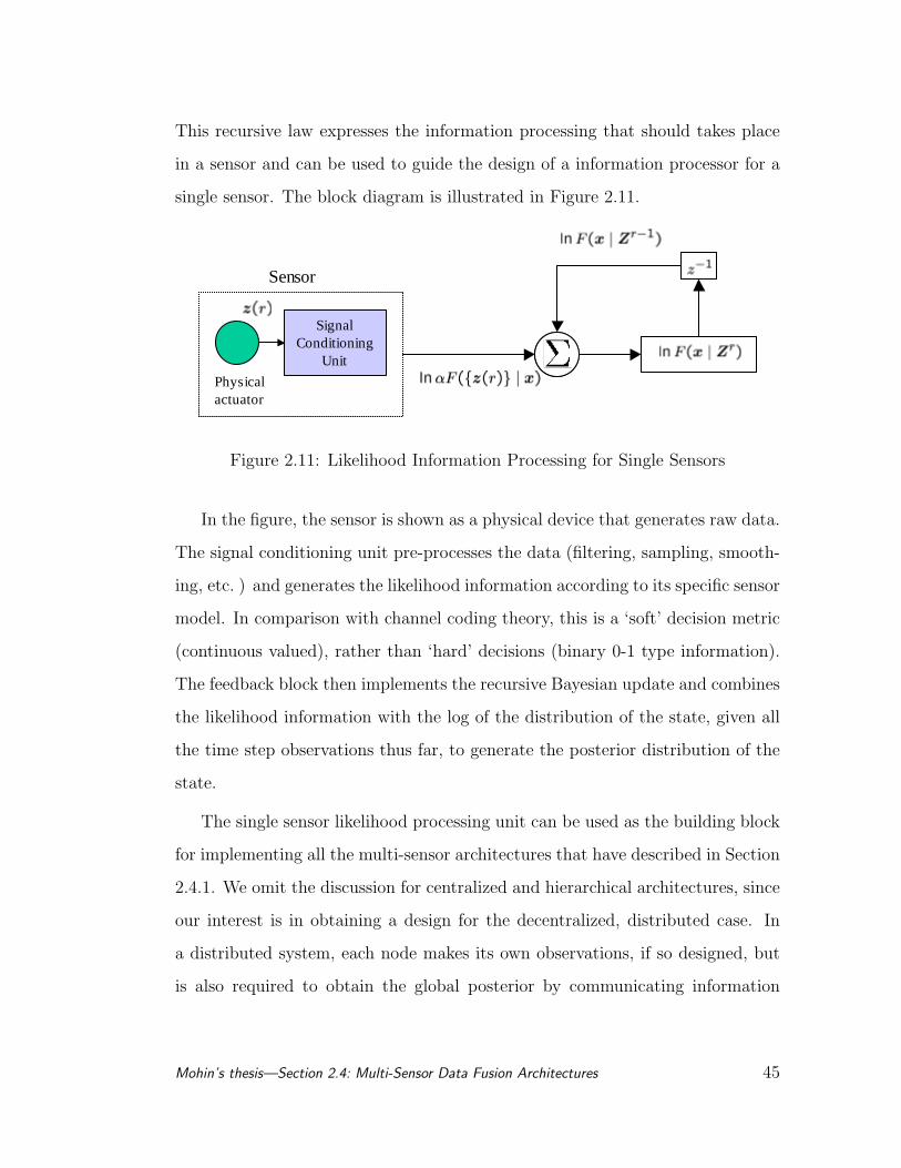
This recursive law expresses the information processing that should takes place

in a sensor and can be used to guide the design of a information processor for a

single sensor. The block diagram is illustrated in Figure 2.11.

Signal Conditioning

Unit

Physical actuator

Signal Conditioning

Unit

Physical actuator

Sensor

Figure 2.11: Likelihood Information Processing for Single Sensors

In the figure, the sensor is shown as a physical device that generates raw data.

The signal conditioning unit pre-processes the data (filtering, sampling, smooth-

ing, etc. ) and generates the likelihood information according to its specific sensor

model. In comparison with channel coding theory, this is a ‘soft’ decision metric

(continuous valued), rather than ‘hard’ decisions (binary 0-1 type information).

The feedback block then implements the recursive Bayesian update and combines

the likelihood information with the log of the distribution of the state, given all

the time step observations thus far, to generate the posterior distribution of the

state.

The single sensor likelihood processing unit can be used as the building block

for implementing all the multi-sensor architectures that have described in Section

2.4.1. We omit the discussion for centralized and hierarchical architectures, since

our interest is in obtaining a design for the decentralized, distributed case. In

a distributed system, each node makes its own observations, if so designed, but

is also required to obtain the global posterior by communicating information


with the other observers in the system. If the system is fully connected, then

each node has access to every other node’s information, so the global posterior

computation should be identical at each node. However, this situation is neither

always feasible (the network may not be fully connected), nor always desired

(only a subset of a large number of sensor nodes may be involved in a particular

observation scenario).

In the discussion that follows, we assume that the state of nature being ob-

served at sensor i is xi. Then, for the case of multi-sensor systems designed

to operate under the Likelihood Opinion Pool data fusion rule, we have seen in

Section 2.2.4, Equation (2.29) that the fusion rule is simply a product of the

likelihoods (or a sum of the log-likelihoods). Therefore, at each sensor i, the data

fusion can be performed by a simple log update relationship as follows:

ln F (xi | Zr) = ln F (xi | Zr−1) +∑

j

ln [αjF (zj(r) | xj]︸︷︷︸communicated

(2.42)

Furthermore, each sensor node i also computes a local partial posterior distribu-

tion based only on the local observation information and a global prior:

ln F (xi | Zr−1 ∪ zi(r)) = ln F (xi | Zr−1) + ln[αiF (zi(r) | xi)] (2.43)

This partial posterior is a summation of information known globally before

time step r and the information that the sensor i contributes at time r. This can

be exploited by the other data processors in the network to gauge the quality of

the information that the sensor provides—a sort of fault detection in a distributed

environment.

Thus, the main result of this section—the general architecture for multi-sensor

data fusion using the likelihood opinion pool—can be summarized and pictured

as shown in Figure 2.12.


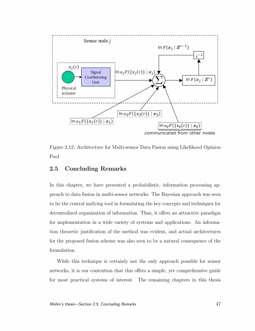
Signal Conditioning

Unit

Physical actuator

Signal Conditioning

Unit

Physical actuator

Sensor node j

Figure 2.12: Architecture for Multi-sensor Data Fusion using Likelihood Opinion

Pool

2.5 Concluding Remarks

In this chapter, we have presented a probabilistic, information processing ap-

proach to data fusion in multi-sensor networks. The Bayesian approach was seen

to be the central unifying tool in formulating the key concepts and techniques for

decentralized organization of information. Thus, it offers an attractive paradigm

for implementation in a wide variety of systems and applications. An informa-

tion theoretic justification of the method was evident, and actual architectures

for the proposed fusion scheme was also seen to be a natural consequence of the

formulation.

While this technique is certainly not the only approach possible for sensor

networks, it is our contention that this offers a simple, yet comprehensive guide

for most practical systems of interest. The remaining chapters in this thesis

Mohin’s thesis—Section 2.5: Concluding Remarks 47

explore some of these practical issues in greater detail, concentrating on the

physical and network layer aspects of the problem of decentralized information

processing in wireless networks.

Mohin’s thesis—Section 2.5: Concluding Remarks 48

CHAPTER 3

Information Processing Bounds in Data

Networks: Simplified Cases

In the previous chapter, we considered information processing as the end goal

of all network and communication management tasks, which we collectively to

referred to as network resource administration (Section 2.1). Needless to say, inef-

ficient adminstration of networking resources and tasks, such as routing, medium

access control (MAC), physical layer issues (e.g. coding, modulation, power levels,

etc.) can make the whole information processing objective moot. Thus, general

bounds are desirable on the what is, and what is not, possible with a given set

of resources and constraints, for a given set of objectives. The proper match

between the two is the entire field of communication and network engineering.

Many results have been derived over the last half century with regards to the

bounds on performance of protocols at all levels of the OSI stack ([81, 74, 91]).

In this chapter we consider two special cases; the rate distortion region for the n-

Helper Gaussian network, and the asymptotic delay in random wireless networks.

Specifically, we consider the wireless sensor and information processing net-

works of Chapter 2 from an information theory point of view and bound the

rate distortion region for the special case of correlated Gaussian sources where n

sources provides partial side information to one main source. We show that an

explicit expression for the lower bound of the rate is possible. This is discussed

49

in Section 3.1. The main utility of this result is to enable comparison of the

performance of the practical data fusion schemes that were suggested in Section

2.4.2 with the theoretically predicted limits.

In the context of quality of service (QoS) for wireless networks, we also con-

sider the problem of delay that information packets encounter as a result of the

resource administration tasks undertaken by the various protocol layers in practi-

cal networks. Despite voluminous analysis of the many different types of routing,

medium access, and physical layer techniques and protocols, there remains a need

to analytically model the entire network stack cohesively to evaluate end-to-end

performance bounds. Hence, it is still not clear what the performance limits of

such networks are likely to be, especially when scaled to large numbers of nodes.

We tackle a simplified version of this scenario by considering parameters and con-

ditions that can be extended to the limit, to simplify the analytical difficulties,

and present a limiting study of the ‘average’ delay characteristics for information

packets in mobile networks. We show that, in the limit, the delay observed per

information bit that is transmitted by a ‘typical’ node in the network averages

essentially to the order of O (√

n ) as a first approximation. This is discussed in

Section 3.2.1.

3.1 Rate Distortion of n-Helper Gaussian Sources

The main problem that this section addresses is: what data rates can be sup-

ported for data fusion in a sensor network, given a specified data distortion level

that can be tolerated? Unfortunately, an exact answer to this question is not

available in the general case, and thus we have considered the specific case of

correlated Gaussian sources in this paper.

Mohin’s thesis—Section 3.1: Rate Distortion of n-Helper Gaussian

Sources 50

The motivation for this problem comes from performing distributed detec-

tion of phenomena. As discussed in detail in Chapter 2, it is well known from

the theory of distributed detection that higher reliability and lower probability

of detection error can be achieved when observation data from multiple, dis-

tributed sources is intelligently fused in a decision making algorithm, rather than

using a single observation data set [96]. This, coupled with the fact that fabri-

cation technological advances have made low-cost sensors incorporating wireless

transceivers, signal processing and sensing in one integrated package a desirable

low-cost option, it is inevitable that such devices will be widely used in detec-

tion applications such as security, monitoring, diagnostic, remote exploration etc.

This has given rise to the development of wireless integrated networked sensors

(WINS) [73], as shown in general in Figure 3.1.

However, the effective deployment of such distributed processing systems in-

troduces some significant design issues, most notably: networking and commu-

nication protocols, transmission channel and power constraints, and scalability,

among others [72, 73],. However, it is also evident that some fundamental limits

are required to assess the optimality of any system design with regard to the

“best design”. Thus, an information theoretic analysis of the system is required.

We have assumed that the primary constraint for our applications of interest is

power.

A WINS system invokes a multi-terminal analysis, as diagrammed in 3.1.

For this type of a system, all the traditional types of multi-terminal channels

considered in information theory appear: the multiple access channel (commu-

nication pathways shown in 3.1 numbered as 1), the broadcast channel (2), the

relay and interference channel (3), etc. [28]. Additionally, the channel may be

fading or more complex. Unfortunately, in the absence of a general information


Sources 51

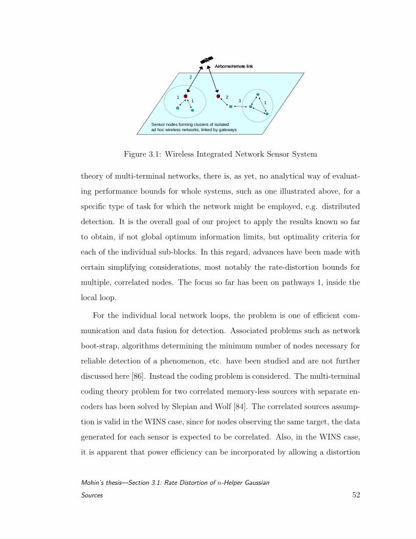
Airborne/remote link

11 13

2

2

Sensor nodes forming clusters of isolated ad hoc wireless networks, linked by gateways

Airborne/remote link

11 13

2

2

Sensor nodes forming clusters of isolated ad hoc wireless networks, linked by gateways

Figure 3.1: Wireless Integrated Network Sensor System

theory of multi-terminal networks, there is, as yet, no analytical way of evaluat-

ing performance bounds for whole systems, such as one illustrated above, for a

specific type of task for which the network might be employed, e.g. distributed

detection. It is the overall goal of our project to apply the results known so far

to obtain, if not global optimum information limits, but optimality criteria for

each of the individual sub-blocks. In this regard, advances have been made with

certain simplifying considerations, most notably the rate-distortion bounds for

multiple, correlated nodes. The focus so far has been on pathways 1, inside the

local loop.

For the individual local network loops, the problem is one of efficient com-

munication and data fusion for detection. Associated problems such as network

boot-strap, algorithms determining the minimum number of nodes necessary for

reliable detection of a phenomenon, etc. have been studied and are not further

discussed here [86]. Instead the coding problem is considered. The multi-terminal

coding theory problem for two correlated memory-less sources with separate en-

coders has been solved by Slepian and Wolf [84]. The correlated sources assump-

tion is valid in the WINS case, since for nodes observing the same target, the data

generated for each sensor is expected to be correlated. Also, in the WINS case,

it is apparent that power efficiency can be incorporated by allowing a distortion


Sources 52

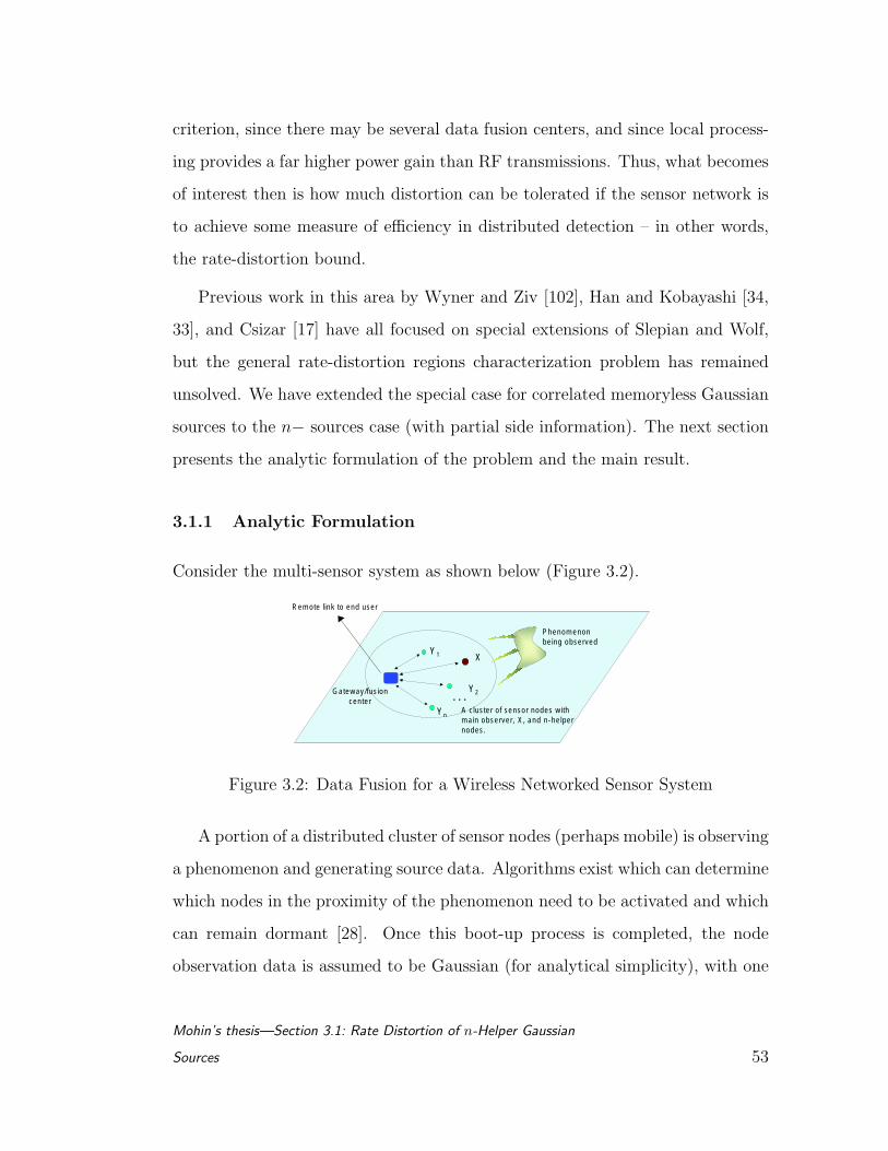
criterion, since there may be several data fusion centers, and since local process-

ing provides a far higher power gain than RF transmissions. Thus, what becomes

of interest then is how much distortion can be tolerated if the sensor network is

to achieve some measure of efficiency in distributed detection – in other words,

the rate-distortion bound.

Previous work in this area by Wyner and Ziv [102], Han and Kobayashi [34,

33], and Csizar [17] have all focused on special extensions of Slepian and Wolf,

but the general rate-distortion regions characterization problem has remained

unsolved. We have extended the special case for correlated memoryless Gaussian

sources to the n− sources case (with partial side information). The next section

presents the analytic formulation of the problem and the main result.

3.1.1 Analytic Formulation

Consider the multi-sensor system as shown below (Figure 3.2).

XY1

. . .A cluster of sensor nodes with main observer, X, and n-helper nodes.

Remote link to end user

Gateway/fusioncenter

Y2

Yn

Phenomenon being observed

Figure 3.2: Data Fusion for a Wireless Networked Sensor System

A portion of a distributed cluster of sensor nodes (perhaps mobile) is observing

a phenomenon and generating source data. Algorithms exist which can determine

which nodes in the proximity of the phenomenon need to be activated and which

can remain dormant [28]. Once this boot-up process is completed, the node

observation data is assumed to be Gaussian (for analytical simplicity), with one


Sources 53

data node acting as the main data source (e.g. that which is closest to the

phenomenon), and the remaining nodes generating correlated data. The coding

challenge is then to determine appropriate codes and data rates such that the

gateway/data-fusion center can reproduce the data from the main node using the

remaining nodes as sources of partial side information, subject to some distortion

criteria.

Thus for a main source, X, and n correlated sources, Yi, such that

Xt, Y1t, · · ·Ynt∞t=1

are stationary Gaussian memoryless sources, for each observation time, t=1, 2, 3,

..., we let the random (n+1)-tuplet (Xt, Y1t, · · ·Ynt) take values in X×Y1×· · ·Yn.

The joint probability density function is given by the usual expression for the

multi-dimensional Gaussian probability density function, where the covariance

matrix can be denoted as:

σ2X ρXY1σXσY1 · · · ρXYnσXσYn

ρXY1σXσY1 σ2Y1

· · · ρY1YnσY1σYn

......

. . ....

ρXYnσXσYn ρY1YnσXσY1 · · · σ2Yn

(3.1)

We can write independent copies of Xt∞t=1 as Xn = X1, X2, · · · , Xn and

similarly for Yt∞t=1, k=1,2,. . . ,n. Next, we consider a coding system where data

sequences Xn, Y n, Zn are separately encoded to ϕ1(Xn), ϕ1(Y

n), ϕ1(Zn) and

sent to the information processing / data fusion center. The decoder function,

ψ = (ψ1, ψ2, ψ3), observes the (n + 1)−tuplet ϕ1(Xn), ϕ1(Y

n), ϕ1(Zn) and

estimates(Xn, Y n, Zn

). We let =n,δ(R1, R2, R3) denote the set of all such cod-

ing and decoding schemes, (ϕ1, ϕ2, ϕ3, ψ), which can exist with the properties

mentioned above. We take :


Sources 54

d1 : X2 → [0,∞) , d2 : Y 2 → [0,∞) , d3 : Z2 → [0,∞) (3.2)

as the distortion measures, which, in our case, is the squared distortion measure,

and we let the average distortions be ∆1 = E

1n

n∑t=1

d1(Xt, Xt

(similar expres-

sions for the other sources). Then for given positive numbers DX , D1,. . . ,Dn, a

rate (n + 1)-tuplet RX , R1,. . . ,Rn, , is admissible if for any δ > 0, n ≥ n0(δ),

there exists a (n+2)-tuplet (ϕ1, ϕ2, ϕ3, ψ) ∈ =n,δ(R1, R2, R3), such that ∆i ≤Di + δ, i = 1, 2, 3.

In our specific case, we do not care about the reproduction of the Yi’s, so the

Di’s can be large. Rather, the Yi’s act as helpers to reproduce X by providing side

information at the data fusion node. This is the so called n-helper case. Then for

an encoding system using the Yi,’s as n-helpers, the rate-distortion region given

by:

<(DX , D1, · · ·Dn) = (RX , R1, · · ·Rn) : (RX , R1, · · ·Rn) is admissible (3.3)

for a given set of rates and distortion measures, is desired. For the special case

of the correlated Gaussian sources, extending previous results [28, 17], we now

state our main result for an admissible rate.

Theorem 3.1. We consider the following encoding functions:

ϕX : Xm → ℵ1 = 1, · · · , C1 · · ·ϕi : Y mi → ℵi = 1, · · · , Ci

to be such that the rate constraints being satisfied are

1

mlog Ci ≤ Ri + δ, i = X, 1, 2, . . . n.

then for an admissible rate (RX , R1, R2, · · ·Rn), and for some D′is > 0, the n-

helper system data rates for correlated Gaussian sources can be fused to yield


Sources 55

an effective date rate (with respect to source X) satisfying the following lower

bound

RX ≥ 1

2log

σ2X

DX

·[

n∏

k=1

(1− ρ2

XYk+ ρ2

XYk· 2−2Rk

)] 1

n

. (3.4)

This is the desired rate distortion region.

Proof:

The method of employing joint weakly δ-typical tuplet, based on typical se-

quences, is used in the proofs of the characterization, rather than a measure-

theoretic approach [17]. We assume that an admissible set of rates exists, and we

let

Wx = ϕX (Xn) , Wi = ϕi (Yn) .

Then:

n(Rx + δ) ≥ log(C1) ≥ H(W1) ≥ I(Xn; Xn)− 1

n

n∑

k=1

I(Xn; Wk) (3.5)

n(Ri + δ) ≥ log(Ci) ≥ H(Wi) ≥ I(Y ni ; Wi) (3.6)

Note that Wi → Y ni → Xn forms a Markov Chain, thus defining:

Fn(D) = infXn:∆1≤D

1

nI(Xn; Xn) (3.7)

Gi(R) = sup8>>><>>>:

Wi:1n

I(Y ni ;Wi)≤R

Wi→Y ni →Xn

9>>>=>>>;

1

nI(Xn; Wi) (3.8)

we get:

RX + δ ≥ Fn(DX + δ)− 1

n

n∑

k=1

Gk(Rk + δ) (3.9)

By the Gaussian property of the sources, and concavity of the logarithm

function, we get:

1n

I(Xn; Xn

)≥ 1

2log

(σ2

X

D

)⇒ Fn (D) ≥ 1

2log

(σ2

X

D

)(3.10)


Sources 56

Finally, an upper bound of Gi (R) is obtained by an extension of the technique

for the two node case (entropy of the power inequality, monotonicity, Jensen’s

inequality):1

nI (Xn; Wi) ≤ 1

2log

(1

1− ρ2XYi

+ ρ2XYi

· 2−2R

)(3.11)

Substituting the bounds in the expression for Fn (D), we obtain:

RX + δ ≥ Fn(DX + δ)− 1

n

n∑

k=1

Gk(Rk + δ)

≥ 1

2log

(σ2

X

D1 + δ

)+

1

2

n∑

k=1

log(1− ρ2

XYk+ ρ2

XYk· 2−2(Rk+δ)

) 1n

(3.12)

Letting δ → 0, we obtain the final result:

RX ≥ 1

2log

σ2X

DX

·[

n∏

k=1

(1− ρ2

XYk+ ρ2

XYk· 2−2Rk

)] 1

n

. (3.13)

3.1.2 Conclusion

In this section, we have considered the rate distortion problem for a sensor net-

work employing data fusion at a node. The main assumption has been that

the n-helper nodes are all producing correlated Gaussian data, which has then

enabled us to obtain an analytic form for the rate distortion bound. The pri-

mary utility of this result is to compare practical data fusion schemes with the

predicted bounds—in particular, to determine which are the most critical and

sensitive parameters affecting rate and performance of a data fusion scheme in a

network sensor system.

The main limitation of the work is that currently, extensions to the more

‘real-world’ scenario of non-Gaussian sources and channels is not obvious. How-

ever, efforts are underway to formulate numerically solvable versions for the more

realistic scenarios. Our ultimate goal is, in the absence of any tractable analyti-

cal expression, to obtain at least an iterative algorithm, or a convex optimization


Sources 57

form. Ideally, this would allow us to accurately predict maximum rate/ minimum

distortion pairs for a wide variety of channels and sources for random arrange-

ments of sensors. We would also like to be able to investigate various ‘what-if”

scenarios in simulation set-ups for particular types of configurations and coding

implementations.

Thus, we hope eventually to be able to use these bounds to definitively com-

pare various data fusion and network communication schemes for wireless sensor

networks, with regards to their performance and efficiency.

3.2 Asymptotic Delay in Random Wireless Networks

3.2.1 Introduction

As mentioned earlier, ad hoc networks are self-governing, self-organizing, dis-

tributed networks consisting of portable computers, or hosts, that communicate

via a common wireless channel [32]. Their main advantage is that they can be

rapidly deployed in situations where no wireless communication infrastructure

exits, or where such an infrastructure is difficult or expensive to implement.

Such networks are of great practical and theoretical interest. They are of

practical interest precisely because the future of digital communications will un-

doubtedly be wireless, at least the “last mile” links, and most likely peer-to-peer,

in an ad hoc fashion. They are of theoretical interest, because the rigorous anal-

ysis of the performance issues for wireless networks is still not complete. There

has been a large amount of research conducted regarding the information theory

of multi-user channels, However, many open problems still remain in the field of

network information theory, and the issues regarding performance bounds for de-

lay, system capacity, achievable rates, suitable codes etc. are chief among them.

Mohin’s thesis—Section 3.2: Asymptotic Delay in Random Wireless

Networks 58

As pointed out in [19], a satisfactory union among the two disciplines is not yet

complete.

One recent study that has gone a long way towards that goal is [31], in which

the authors determined the uniform achievable rates for nodes in an asymptoti-

cally large ad hoc network, as well as several bounds for the capacity of the net-

work under different protocols. However, the problem of determining the“average

delay” in such arbitrary networks still has not been tackled in a general manner.

This is of interest since in practical networks, bounds on delay have a direct rela-

tionship to the quality of service that large networks can expect to deliver. To the

designer of such networks, it can provide insight as to the limits of performance

and what we can expect from such networks, and how the myriad of currently

available protocols scale to the theoretical limit.

With regards to prior art, in [15, 16], the author studies the delay character-

istics of specific network elements which can be interconnected to form complex

networks. However, this yields tractable analysis only when the input traffic

characteristics obey certain burstiness properties, and cannot be readily applied

to the wireless case, or used to compute an overall ‘average’ delay. In the studies

done in [3] and [91], the authors look specifically at queuing and its impact on

information flow in a network, but once again, the analysis does not lend itself

easily to a general analysis of the delay in a mobile ad hoc network. The tech-

niques are elegant, but further research is required to determine if they can be

modified to apply in a straightforward manner to the mobile wireless case.

In this section, we instead undertake a simplified study of this problem and

attempt to formulate a very simple bound for a restricted scenario. We propose

to use the results of [31] and a probability result derived in [61] and attempt

to extract a first order bound. Specifically, we consider the average delay that


Networks 59

bits generated by arbitrary nodes in the network can expect to experience while

being routed from source to destination, as the nodes in the network increase

asymptotically. The following section contains a brief description of the analysis.

3.2.2 Analysis

We consider the same scenario as the author in [61], some details of which are

reproduced below. n nodes are randomly distributed over an unbounded area.

The x and y coordinates of the node locations are assumed to have zero-mean

Gaussian distributions, for the purposes of analytical derivation. Then assuming

that the transmission range of each mobile is R, and the Gaussian distribution

has variance σ2, then the probability density function (pdf) of the link distance

between two arbitrary nodes is given by:

pr(r) =r

2σ2e−r2/4σ2

. (3.14)

The probability of a 2-hop connection between an arbitrary source and desti-

nation pair, separated by a distance r, is then given by:

P2 = P1 → 2 in 2 hops

= PR < r < 2R and at least 1 other node in area of intersection

=

∫dx1

∫dy1

∫dx2

∫dy2 px,y(x1, y1, x2, y2)

×[1−

[1−

∫dx3

∫dy3px,y(x3, y3)

]n−2]

(3.15)

As n approaches infinity, the expression given above can be approximated

with the following upper bound (derivation in [61]):

P2 <

∫ R2/σ2

R2/4σ2

e−ν(1− 0) dν (3.16)


Networks 60

which simplifies to (e−R2/4σ2−e−R2/σ2) , P2∞. It can then be shown by a similar

argument that the asymptotic probability of an m-hop connection is given by:

Pm < e−(m−1)2R2/4σ2 − e−m2R2/4σ2 , Pm∞ (3.17)

and therefore an upper bound on the average number of hops between the node

pairs can be calculated from:

Eh =n−1∑m=1

mPm <

∞∑m=1

mPm∞. (3.18)

In [61], it is seen by numerical analysis that this expression converges to a

nearly linear function of the ratio of node dispersion parameter (standard devi-

ation of the Gaussian) to transmission range. Thus, using non-linear regression

techniques, and subsequent linearization, we are left with the following remark-

ably simple approximation for the asymptotic average number of hops that an

‘average’ data bit takes from and ‘average’ source to its intended destination node,

for an arbitrary wireless network with Gaussian (spatially) distributed nodes:

Eh < 0.5 + 1.772(σ/R). (3.19)

In terms of actual distance, we can simply multiply by the transmission range

of each node R, to obtain the average hop distance per transmitted bit. Note

that this result is not limited by any specific routing, access, modulation proto-

col. We can now utilize this result and the asymptotic capacity results for the

Physical Model (arbitrary) network as in [31], with some appropriate modifica-

tions regarding domain geometry. It has been shown in [31] that the transport

capacity of such an arbitrary network of n nodes scattered in a disk of unit area

is of the order O (W√

n ) bit-meters per second (which is equal to on the order


Networks 61

of O (W/√

n ) bit-meters per second per node). Since the average hop distance

given in 3.19 is for an unbounded disk, we make the following observation. The

nodes in the scenario described earlier are zero-mean Gaussian distributed, there-

fore, 99.7% of all the nodes are expected to lie within a 3σ radius of the center.

The resulting area of the disk of radius 3σ disk is 9πσ2. We can therefore scale

the results in [31] by this factor.

Another issue is the fact that the capacity results are cited for uniform distri-

bution over the unit area disk, whereas the hop distance calculations were done

for a Gaussian distribution. Once again, in the limit of n approaching very large

values, we can appeal to the central limit theorem regarding node separation

distribution for the two cases and equate them as a first order approximation for

asymptotic analysis.

Thus, we finally have a first order approximation for the expected delay a bit

experiences in an arbitrary wireless network.

D ∼ O

R

(0.5 +

1.772σ

R

) /9πσ2W√

n

= O

√n

Wσ2· (0.056πR + 0.197π)

(3.20)

where R is the transmission radius of a representative node, σ2 is the variance

of each of the x and y coordinate of the Gaussian dispersion, and W is the

feasible transmit rate of each node. Since we are interested in the asymptotic

relationship of the delay to the network parameters, we can further ignore all the

constant factors in the expression above, and are thus left with the following order

expression for the ‘average’ delay experienced by a random bit in the network:

D ∼ O

R

Wσ2· √n

(3.21)


Networks 62

As a function of the network size alone, we obtain:

D ∼ O(√

n)

(3.22)

3.2.3 Concluding Remarks

The scenario as discussed above is somewhat limited in scope since the disper-

sion pattern was fixed to be Gaussian and node capabilities were limited since the

impact of mobility was not considered. Additionally, the results we relied upon

to derive the order expression for the delay assumes a globally optimal scheme

for the routing, medium access, etc., which may not realistic. However, these

assumptions do yield insight and a simple analysis into the typical delay charac-

teristic of bits in the network. A future research direction is to relax some of the

assumptions and observing where/if the analysis become intractable, and what

alternative strategies can be applied, e.g. by incorporating some queuing results

from [3, 91].


Networks 63

CHAPTER 4

Gateway Optimization for Connectivity in

Heterogeneous Multi-Tiered Wireless Networks

In this chapter, the hypothetical data fusion architectures discussed briefly in

Chapter 2 are considered in the context of some real-life, large-scale networks.

Practical issues, which were referred to as sensor organization earlier (Section

2.1.1), we now investigate in terms of performance and associated costs. In par-

ticular, we note the emergence of mobile ad hoc network (MANET) technology,

which allows practical deployment of many of the decentralized information pro-

cessing concepts that have been researched over the last few decades. In this

chapter, we focus on a narrow subset of those concerns: specifically, the issue of

facilitating scalability and range extension in partitioned mobile ad hoc networks.

We propose that to facilitate scalability in and to provide connectivity between

partitions that might occur in wireless networks as a consequence of mobility, we

can envision a ‘range extension’ network that consists of airborne communication

platforms, and satellites. These airborne or satellite nodes will maintain commu-

nication links with specific ‘gateway’ nodes among the mobile ground nodes. To

communicate with a node that is geographically distant or belongs to a differ-

ent network partition, a node can relay its data packets through an appropriate

mobile gateway and via the range extension network. If we envision that the

MANET is divided into different groups and a mobile gateway is deployed for

64

each such group, an objective then, is to determine the trajectory of the mobile

gateway to best serve the ad hoc group to which it belongs, in terms of net-

work performance metrics such as throughput and latency. In this chapter, this

problem of computing the optimal position for a gateway is reduced to a linear

optimization problem by means of some simplifying but realistic assumptions. We

suggest methods that may be deployed to enable the gateway to follow this opti-

mal trajectory as closely as possible (within the practical constraints imposed by

its velocity and maneuverability). Simulation results for various scenarios show

a 10-15% improvement in the throughput and in latency (per group containing a

gateway) if a gateway has a dynamic trajectory whose locus follows the computed

optimal position, as compared to a gateway that is statically placed at a regular

position, or to a gateway that has a random trajectory.

4.1 Introduction

Mobile ad hoc networking technology [32] may be appropriate for linking mo-

bile computers in an office or home environment, deploying wireless sensors in

remote or inhospitable terrain, coordinating disaster relief efforts after natural

catastrophes, or in tactical deployments for situation awareness applications [51].

A major challenge in the wide deployment of MANETs has been in achieving

scalability. Furthermore, due to the range limitations of the nodes in the ad hoc

network, the network might often be divided into isolated partitions. In order to

achieve scalability in terms of efficient communications between geographically

distant nodes or between nodes that belong to different isolated partitions (each

of which is an ad hoc group by itself), it is desirable to provide a supporting

infrastructure in the form of a range extension network. This infrastructure is

also essential to interface the MANET with the Internet.


This range extension network could typically consist of airborne relay nodes or

low earth orbit/geostationary satellites. In order to interface the ad hoc network

with the range extension network, one can envision the deployment of special

gateway nodes in the ad hoc network. These are ‘on-ground’ nodes that might

be more power/processing capable than the other ad hoc nodes on the ground

and are equipped with the appropriate hardware for communicating with the

satellite/airborne nodes. This architecture can therefore be visualized to con-

sist of two layers. The first layer includes the ad hoc network, and the second

includes the range extension network consisting of satellites or airborne nodes.

The mobile gateway provides the interface for the communications between the

two layers and hence we shall call a gateway node a “Cross Layer Communica-

tion Agent” or CCA from this point onwards. Similar architectures have been

previously considered for enabling hierarchical routing or multicasting [44, 2]. In

[44], and [2], topological information is used to build spanning trees rooted at

convenient nodes in the MANET. In [43], the authors have investigated the fea-

sibility of partitioning MANETs into groups with cluster-heads or repositories of

information to enable efficient information dissemination [43]. In contrast, our

objective is the determination of the CCA trajectory that a mobile gateway or

CCA has to follow in order to optimize inter-domain network performance.

A CCA may be assigned to a group of ad hoc nodes or it might be affiliated

with a geographical domain and placed statically at the center of the domain. In

the former case, it links the range extension network with the specific group of

ad hoc nodes. In the latter case, it provides the ad hoc nodes within the specific

geographical domain with a link to the range extension network. If the CCA is

mobile and is affiliated with an ad hoc team of mobile units, the question arises

as to where the CCA ought to be located relative to the mobile units. In other

words, the objective is to specify the locus of the position that a mobile CCA


is to follow and the rules that govern this trajectory with respect to the relative

motion of the other mobile units. We design a methodology for defining the

CCA trajectory based upon the location, loading, etc. of the other mobile nodes

in the ad hoc group that the CCA serves. We show that network performance

improves (for communication involving nodes in different clusters of nodes), in

terms of throughput and latency, if the CCA trajectory is computed based on

our methodology.

We derive a relatively simple analytic formulation for the optimal CCA posi-

tion, which is equivalent to a linear optimization problem. This is discussed in

Section 4.3. We also provide an algorithmic implementation of the formulation,

and discuss the effect of some of the parameters in this section. Various scenarios

are considered for deliberation. In Section 4.4, we estimate the overhead for im-

plementing this architecture with the aid of typically used media access control

(MAC) and routing protocols. We also investigate the computational complex-

ity of our CCA trajectory definition algorithm. In Section 4.5, we discuss our

simulation framework and discuss the results. We conclude in the final section.

4.2 System Model

We motivate the discussion of the system architecture that we laid out in the

previous section in the context of the following scenario. Consider separate groups

of mobile ad hoc nodes operating in a terrain with blockages and deployment area

restrictions (e.g. troop divisions deployed in a mountainous area). Each group

would have one or more CCAs capable of communicating with an airborne or

satellite node with which it has a direct line of sight connection. As an example,

in Figure 4.1, we have considered two isolated groups of mobile nodes, each

forming a MANET by themselves, and each having its own CCA. The ad hoc

Mohin’s thesis—Section 4.2: System Model 67

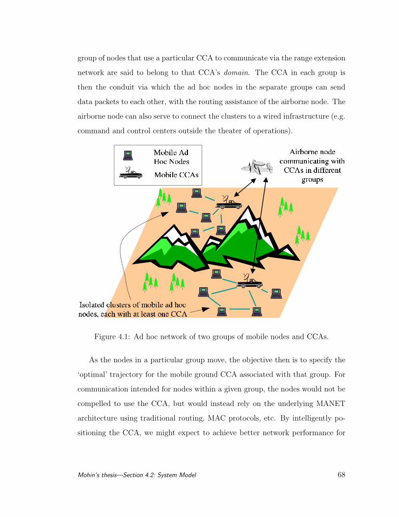
group of nodes that use a particular CCA to communicate via the range extension

network are said to belong to that CCA’s domain. The CCA in each group is

then the conduit via which the ad hoc nodes in the separate groups can send

data packets to each other, with the routing assistance of the airborne node. The

airborne node can also serve to connect the clusters to a wired infrastructure (e.g.

command and control centers outside the theater of operations).

Figure 4.1: Ad hoc network of two groups of mobile nodes and CCAs.

As the nodes in a particular group move, the objective then is to specify the

‘optimal’ trajectory for the mobile ground CCA associated with that group. For

communication intended for nodes within a given group, the nodes would not be

compelled to use the CCA, but would instead rely on the underlying MANET

architecture using traditional routing, MAC protocols, etc. By intelligently po-

sitioning the CCA, we might expect to achieve better network performance for


inter -domain node communications, (i.e. data communication between nodes

that are in the domains of different, possibly geographically isolated CCAs) than

if the CCA were allowed to move randomly with respect to the nodes it its do-

main.

We can assume any suitable mobility model for depicting the motion of the

ad hoc nodes [37]. Thus, some of the nodes may be statically deployed (sensor

nodes) or, the nodes may move according to a random waypoint model [41]; or,

they may move according to a model in which they approximately follow one

particular node that is considered the ‘leader’, etc.

The terrain in which the MANETs are deployed may contain regions where

either the node, or the CCA, or both, cannot reside. These can be regions where,

e.g., channel impediments create radio nulls, or hazard zones which expose the

CCA or specific nodes to harm (in tactical deployments), or where the terrain is

inaccessible, etc. We refer to these regions as blockages.

The performance metrics that could potentially be improved by optimizing

the CCA trajectory include, but may not be limited to, the following:

• inter-domain network data throughput

• inter-domain network packet transport delay

• total power expended (or maximum power consumed per packet/bit per

node in the CCA)

• data transmission reliability (packet drop/error rate)

• volume of the network control messages and resulting signaling overhead.

The procedure by which the weighted centroid is computed requires the fol-

lowing:


1. Each node is equipped with a GPS device that enables the node to deter-

mine its position.

2. Each node can estimate its offered load in real time

3. Terrain information (such as specific coordinates or boundaries of radio null

regions where radio signals cannot propagate, inaccessible terrain, etc.)

is available at each CCA. This can easily be made available at network

inception1.

The details of the actual communication mechanisms that enable the MANET

to function are not directly relevant in the development of our analytical for-

mulation for computing the optimum trajectory that our CCA ought to follow

(Section 4.3). For intra-domain node communications (i.e. communication be-

tween nodes that are in the domain of the same CCA), the MANET could rely

on well-established protocols such as the IEEE 802.11 MAC protocol for media

access control [54], DSR, DSDV, or AODV for routing [41, 69], etc. to establish

and maintain connectivity. For inter -domain node communications, data will

have to be routed through the CCA and via the range extension network.

4.3 CCA Trajectory Update Algorithm: Formulation and

Analysis

In this section we describe the algorithm for determining the trajectory of mobile

CCAs such that it is optimal in terms of ‘relative position’ with respect to the

group of ad hoc nodes that it serves. By having the CCA follow the trajectory

1Position based schemes have previously been suggested and studied for ad hoc networks,[44], [2].

Mohin’s thesis—Section 4.3: CCA Trajectory Update Algorithm:

Formulation and Analysis 70

determined by this algorithm, we expect (and later show by means of simula-

tions) that we will achieve a significant improvement in network performance, in

comparison with a scheme that has static CCAs or has the CCAs follow a trajec-

tory defined by a random way-point model. We describe our algorithm assuming

that there is single CCA per domain in Section 4.3.1. However, it is possible for

several nodes among a cluster of nodes to be capable of communications with the

range extension network and hence any of these nodes could assume the role of a

CCA. Fortunately, in all these cases, the base algorithm that we propose remains

unchanged. Increased layers of complexity can be added to the base algorithm

to enable the CCAs to participate in node ‘hand-off’ as in cellular networks, or

to intelligently share the load generated by the nodes in the overlapping regions

of intersecting domains. These features may be exploited to achieve further per-

formance improvements. A brief discussion of the possibilities is presented in

Section 4.3.2.1.

4.3.1 Node Domains Containing a Single CCA

As mentioned earlier, one might expect that the performance of the network

would be best if we could optimally position the CCA within the group of ad

hoc nodes that it belongs to. We refer to this optimal position as the weighted

geographic centroid. This section describes the procedure that computes this

weighted centroid. We formulate an optimization problem that the CCA solves

periodically with the help of information that it has gathered from the other ad

hoc nodes, to determine its trajectory. The parameters that the CCA can take

into account in formulating the optimization problem could include node posi-

tions, each node’s offered load, data traffic patterns, priority of the generated

traffic, the channel signal to interference noise ratio (SIR), among others. The



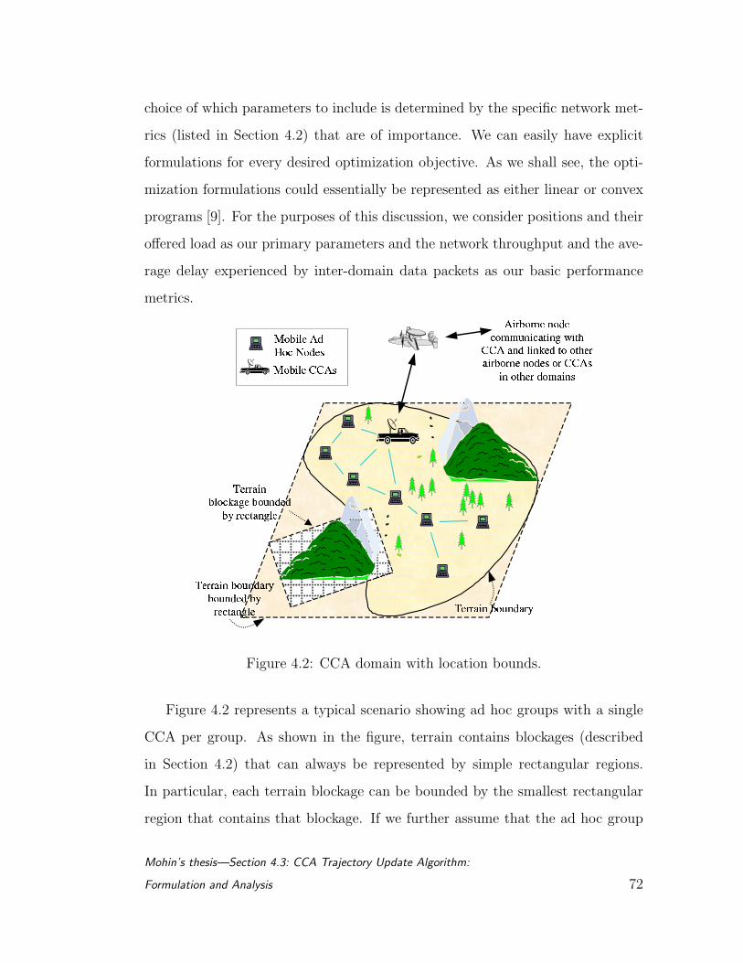
choice of which parameters to include is determined by the specific network met-

rics (listed in Section 4.2) that are of importance. We can easily have explicit

formulations for every desired optimization objective. As we shall see, the opti-

mization formulations could essentially be represented as either linear or convex

programs [9]. For the purposes of this discussion, we consider positions and their

offered load as our primary parameters and the network throughput and the ave-

rage delay experienced by inter-domain data packets as our basic performance

metrics.

Figure 4.2: CCA domain with location bounds.

Figure 4.2 represents a typical scenario showing ad hoc groups with a single

CCA per group. As shown in the figure, terrain contains blockages (described

in Section 4.2) that can always be represented by simple rectangular regions.

In particular, each terrain blockage can be bounded by the smallest rectangular

region that contains that blockage. If we further assume that the ad hoc group



is deployed in a finite area which represents the ‘domain’ of a CCA, then the

area of deployment may also be similarly bounded by a rectangular region. This

representation is useful since the constraints that govern the position of a CCA

can then be described by simple linear equations (based on the coordinates of

the rectangle boundaries). Note that it is extremely hard if not impossible to

characterize the arbitrary geometries that these regions might have by exact

mathematical expressions. Thus, our model for the region over which the CCA

can move consists of a rectangular area with smaller rectangular regions marked

as ‘no-go’ areas.

A fundamental characteristic of MANETs, (also shown in Figure 4.2) is that,

not all the nodes in the domain have a direct link to the CCA. Some nodes will be

outside the single-hop radio range of the CCA and will have to route their data

packets to the CCA via multiple hops through other ad hoc nodes2. The cost

function that we use in computing the weighted geographic centroid takes the

offered load of the individual nodes and the priorities of the packets generated at

each node into account. This ensures that the CCA is closest to the most heavily

loaded nodes, or to the nodes that generate packets of the highest priority, as

the requirement might be. Thus, when all packets are of the same priority, the

CCA is positioned such that most of the data packets reach the CCA in a single

hop, thereby ensuring a better utilization of the available resources. In the case

wherein nodes generate packets of different priorities, the CCA’s position would

ensure that most of the higher priority packets would reach the CCA in a single

hop.

2These data packets are destined for nodes in other domains and thus must be routedthrough the CCA to the range extension network.



4.3.1.1 Optimization Formulation

We assume that the CCA acquires the coordinates of each node in its domain,

that needs to send inter-domain data packets3. The weighted centroid is simply a

factored distance norm, and the constraints are linear inequalities. For a domain

with n nodes, the optimization problem can be formulated as:

minimizen∑

i=1

f(τi, ρi) · |x0 − xi| (4.1)

subject to w1 ≤ x0 ≤ w2 (4.2)

x0 ≥ b2k (4.3)

x0 ≤ b1k (4.4)

The optimization variable in the norm minimization expression, Equation. 4.1,

is the CCA position, represented by the 2-D (ground) position vector, x0, with

reference to any suitable origin in the terrain of interest. The other xi’s represent

the coordinate vectors of the mobile nodes with respect to the same origin. The

values of xi’s are obtained at each sampling instant and a new value of x0 is

computed. The weighting factor, f(ρi, τi) is a user defined function that depends

on the ith node’s load, ρi, and priority, τi. Note that when we use the term load,

we in fact refer to the data traffic that the ith node wants to send to nodes in other

domains. We do not consider the data load due to intra-domain communication

among the nodes, although this may affect the available bandwidth for inter-

domain communications4. Depending on the type of traffic being generated by

the nodes, the function f(ρi, τi) can be defined appropriately to reflect CBR, or

3We will discuss the technique by which this acquisition is realized and the resulting overheadincurred involved in Section 4.4.

4Alternatively, we can assume that separate channels exist for intra-domain and inter-domaincommunications.



variable bit rate (VBR) traffic and with or without defined priorities. The terms

wi are the vector coordinates representing the outer rectangle circumscribing the

domain (bottom left and the top right points), and bik’s are similar vectors that

represent the boundary of the kth blockage. Therefore, we are minimizing the sum

of the weighted geometric distance from the CCA to each of the nodes, subject

to the boundary and blockage constraints.

As stated earlier, this problem is a non-linear optimization problem [8]. How-

ever, if we ensure that the cost function is the L2 norm, since the constraints are

linear, the problem is a convex program (all norm functions are convex). This

problem, therefore, has a global optimum and any of the standard convex opti-

mization algorithms can be used to find the optimal position, x0 for the CCA (e.g.

steepest descent, Newton’s methods, etc. [8], [9])5. Furthermore, the convex op-

timization problem itself can be easily transformed into a simple linear program

(LP) and the cost function can be replaced by an equivalent linear cost function.

The resulting LP can then be solved far more efficiently via modern interior point

methods [59]. An implementation would require the CCA to perform the CCA

Trajectory Update Algorithm which is as follows.

Algorithm 4.1. CCA Trajectory Update Algorithm

• Input constants (set ‘a priori’): terrain and blockage boundaries, sampling

times, optimization metric of interest.

• Output : optimum CCA location computed at specific sampling times.

• While nodes in the domain have inter-domain data packets to send, DO:

5Since the problem is formulated as a convex program, the solution is found by numericalmethods.



1. Collect or estimate the position of each node, xi, at each sampling

instant.

2. Collect from each node, an estimate of its current load and the priority

that it desires6.

3. Perform a local computation to solve the LP equivalent to the opti-

mization problem in Equation 4.1 and obtain optimum CCA location

for that sampling instant.

4. Move towards the optimal location in the most suitable manner, as

allowed by the physical constraints7.

5. REPEAT (at next sampling instant)

The motion of the CCA can be further governed by certain rules to prevent

race conditions and such. As an example, one can have a hysteresis rule that helps

to prevent excessive CCA sensitivity, wherein a computed ‘new’ CCA location

has be greater than a minimum of some pre-specified δ units from the present

location before we decide to move the CCA. Another hysteresis rule might require

the CCA to remain at a newly computed location that it has moved to, for a

specific time period (usually several frame update intervals).

4.3.2 Overlapping CCA Domains

In the methodology discussed so far, we have only considered domains with a

single CCA serving a group of ad hoc nodes. In this section, we consider a

case in which ad hoc nodes have the ability to chose one CCA among a set of

CCAs. Without loss of generality, we can think of this scenario to be equivalent

6The priority is determined by policy and is not discussed further.7The problem of navigating from one location to another, on a 2-dimensional surface with

obstacles with no pre-established paths, is a vast area of research in robotics and is not discussedin this thesis [64].



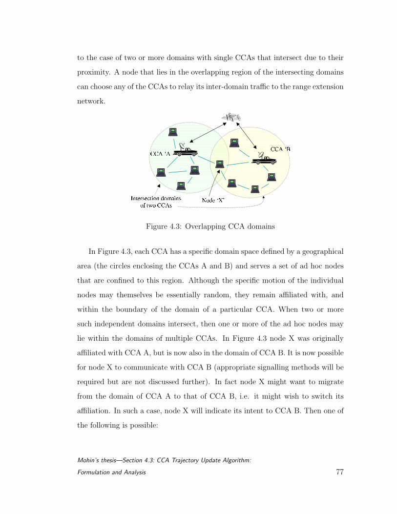
to the case of two or more domains with single CCAs that intersect due to their

proximity. A node that lies in the overlapping region of the intersecting domains

can choose any of the CCAs to relay its inter-domain traffic to the range extension

network.

Figure 4.3: Overlapping CCA domains

In Figure 4.3, each CCA has a specific domain space defined by a geographical

area (the circles enclosing the CCAs A and B) and serves a set of ad hoc nodes

that are confined to this region. Although the specific motion of the individual

nodes may themselves be essentially random, they remain affiliated with, and

within the boundary of the domain of a particular CCA. When two or more

such independent domains intersect, then one or more of the ad hoc nodes may

lie within the domains of multiple CCAs. In Figure 4.3 node X was originally

affiliated with CCA A, but is now also in the domain of CCA B. It is now possible

for node X to communicate with CCA B (appropriate signalling methods will be

required but are not discussed further). In fact node X might want to migrate

from the domain of CCA A to that of CCA B, i.e. it might wish to switch its

affiliation. In such a case, node X will indicate its intent to CCA B. Then one of

the following is possible:



• CCA B may completely ignore this message from node X. In this case, its

trajectory remains unaffected by node X’s message.

• CCA B may agree to relay the data message from/to node X to/from the

range extension network. However, it may not use the control information

from node X (that reflect the position of node X, its offered load, etc.) in

determining its trajectory.

• CCA B may consider node X to temporarily belong to its domain. In

this case, not only does CCA B act as node X’s interface to the range

extension network, but it also takes the position, the offered load, and

other parameters associated with node X into account while determining

its trajectory.

Node X might choose to affiliate with both CCAs A and B. In that case

it transmits an intent message to CCA B as in the previous case and CCA B

could react in accordance to the policy defined in one of the earlier cases, listed

above. If node X is granted partial affiliation by CCA B, it can distribute its

inter-domain load between CCA A and CCA B. Alternatively, the CCAs may

elect to ‘handoff’ selective nodes to each other, as in cellular networks8. Thus,

one might in this case, be able to uniformly balance the inter-domain load in the

network between the CCAs, to the extent possible. This feature and its effect on

the optimal CCA trajectory are described in Section 4.3.2.1.

For each of the cases above, a different optimization rule may be formulated,

and the choice of the rule to use is application specific. However the crucial point

to note is that in spite of this added complexity, the CCAs can still use the same

convex programming formulation that was presented earlier.

8We are assuming that this type of CCA to CCA cooperation can be efficiently done sincethey will both be one hop away from a common aerial/satellite node.



4.3.2.1 Balancing Load Between CCAs

We consider again, the scenario shown in Figure 4.3 as an example. Our objective

is to have the nodes that are in the overlapping regions of the intersection of

multiple CCA domains choose an appropriate CCA so as to evenly distribute

the offered load between the individual domains. We reiterate that by ‘load’ we

refer to the offered data load that is generated due to the packets that are to be

transported via the range extension network.

We assume that the aggregate offered loads at CCA A and B are ρA and

ρB packets per unit time, respectively, and that node X offers a data load of ρ.

Node X can now assist in load balancing by directing the data packets that it

either generates or relays to the appropriate CCA, such that the loads in the two

domains are as close to each other as possible. Thus, if ρA > βρB where β is some

preset threshold, then node X can be instructed to route a fraction α, 0 ≤ α ≤ 1,

of its load to CCA B, while the remaining load (1 − α)ρ is routed to CCA A.

When the two CCA domains have their loads balanced, we essentially have:

ρA − αρ ≈ ρB + (1− α)ρ (4.5)

If node X does not generate enough data packets to satisfy the equation, then

it can route all its packets to CCA B (α = 1) for the duration that it remains in

the overlapping region of the domains of two CCAs. Note that in this discussion,

we assume that the nodes that belong to an ad hoc group will have to stay

with that group. Thus only a temporary switch in CCA affiliation is permitted.

However, it is easy to extend the method to consider permanent migration of

nodes from one CCA’s domain to that of another.

The relatively simple load-balancing technique described in the previous para-

graphs can be extended to include cases in which multiple nodes are in the over-



lapping regions of multiple intersecting domains. In that case, in order to prevent

more than one node from simultaneously initiating load transfer, the CCAs can

coordinate with each other to orchestrate the procedure and instruct the node

that is most heavily loaded to attempt to split its load between the two do-

mains. This procedure may then be iteratively repeated until the loads in the

two domains are balanced.9

4.4 Computational Complexity and Overhead

In implementing our algorithm, it is essential that the incurred overhead in terms

of the number of control message that are exchanged is small. In addition, the

algorithm should be not be computationally expensive since the time taken by

the CCA to compute the optimal location must be small as compared to the

time taken by the CCA to move to that location. In this section, we provide

estimates of the incurred overhead and discuss the computational complexity of

our algorithm.

4.4.1 MAC Protocol, Routing Support and Overhead

For implementing step 3, two tasks are required. First, the identity of the CCA

(e.g. an IP address or MAC address) has to be made known to all the nodes.

This information can be software programmed into all the nodes before network

deployment, or can be broadcast to all the nodes in the domain. This broadcast

is, in fact, required if there are multiple CCAs in the domain, and they are

operating in some cyclic order for specified periods of time. Alternatively, each

node could obtain the address of the CCA on a reactive basis, that is, if and

9This procedure has been simulated and the results are discussed in Section 4.5.

Mohin’s thesis—Section 4.4: Computational Complexity and

Overhead 80

when they have inter-domain packets to send. The overhead in this case is about

the same as in discovering a specific node within a MANET.

Second, the CCA has to obtain state information from all the nodes. If we

consider the Open Systems Interface (OSI) or the TCP/IP layered architecture,

the CCA Trajectory Algorithm can be considered as a program running at the

network layer. It requires the CCA’s network layer to obtain the coordinates, the

offered load, and other parameters from all the other nodes in its domain. To do

so, the CCA would need to broadcast a global query message to all the nodes in

its domain, once every sampling period.

If there are n mobile nodes in the network, then a ‘proactive’ scheme requires

that these nodes transmit an update every sampling period. Then number of

routing messages in the worst case is on the order of O(n2) per sampling period

(assuming flooding is employed to transport these messages) [43]. However, if the

nodes that have inter-domain data to send constitute only a small fraction of the

total number of nodes in the network, say α, then the number of transmissions

will be reduced by this factor to α · n2, which is again O(n2). By intelligently

using the routing tables in order to relay control information, this overhead can

be further reduced.

The sampling period is dependent on the rate at which the topology of the

network changes. This rate depends on the density of the network and the velocity

of the nodes in the network. If a table driven routing protocol is used, routing

updates are required to be disseminated in order to cope with the changes in

topology. The control information that is required for trajectory control may

simply be ‘piggy-backed’ onto the routing update messages10. In fact this control

information may be embedded in the MAC layer ‘hello’ or even piggy-backed onto

10Most of these parameters are usually single 8-bit or 16-bit numbers, per node, so payloaddata length is not an issue.


Overhead 81

the data payload that is routed to the CCA. The CCA would then, appropriately,

extract the appropriate control information. This makes the overhead required for

gathering state information for the algorithm to work to be essentially the same

as, or marginally incremental to the overhead required for enabling the underlying

routing and MAC protocols. For the overhead incurred in deploying various

MANET protocols, the reader is referred to [79]. We note here that in network

simulations, we modified the standard Destination-Sequenced Distance-Vector

Routing (DSDV) protocol [68] by piggy-backing appropriate control information

onto routing update messages.

4.4.2 Optimization Complexity

It is important that the optimization algorithms that we describe in Section

4.3.1.1 not be computationally intensive, since our objective is to administer

trajectory control of the CCA in real-time. In other words, the time that it

takes for the CCA to compute its new position based on the data that it gathers

during a sampling period should be less than the sampling period itself. The

computation of the trajectory involves solving a linear program numerically. It is

well known that modern interior point LP solvers have a worst-case performance

of O(n3) [9], where n is the number of variables in the LP. In our formulation, n

would correspond to the number of nodes in the network. Thus, for a network of

100 nodes, each of which is assumed to generate inter-domain data packets, we

would expect calculations on the order of 1003 or 1 million iterations per update

period. A typical update period is of the order of 0.5 seconds in our simulations.

Currently available ‘off-the-shelf’, inexpensive microprocessors can process on the

order of tens of millions, or hundreds of millions of instructions per second [39].

For a network with 1000 nodes, the complexity increases significantly, requiring 1


Overhead 82

billion iterations per update period. In such cases, however, it is far more efficient

to simply deploy more CCAs, and thus sub-divide the larger domain into smaller

domains of ad hoc networks.

To prevent a possible computational bottleneck at the CCA (which is bur-

dened with both the inter-domain communications of the ad hoc network and the

computation of the optimal position), a dedicated processor may be employed on

each CCA. This would enable the optimization computations and the communi-

cation operations to proceed in parallel.

4.5 Simulation Framework and Results

In order to evaluate the performance of our trajectory control algorithm, we

used the ns-2 network simulator, release 2.1b6 [95] as our primary simulation

platform. We also used Carnegie Mellon University’s code extensions for sup-

porting wireless ad hoc networks. We employed the following implementations

that the code-extensions provide: (a) the link layer and the 802.11 MAC proto-

col modules; (b) CBR, VBR data sources; (c) the physical channel model, which

is the two-ray radio propagation model where signals experience attenuation in

accordance to a fourth power path loss model, and fading/shadowing effects are

not included; (d) a random waypoint motion model to govern the motion of the

mobile nodes. The supporting routing protocol that was used was DSDV [68].

We also conducted simulations with appropriate modifications to the Dynamic

Source Routing (DSR) algorithm [77]. Our results were similar and we omit a

discussion of this due to space limitations.

We created data structures that dynamically maintained the coordinates of

each node and other control information, in the form required for a LP solver.

Mohin’s thesis—Section 4.5: Simulation Framework and Results 83

Next, the LP algorithm itself was integrated into the ns-2 simulation framework

by means of a C function call from the main program code. To implement the

optimization algorithm, we used a modified version of PCx [58]. PCx is a linear

program solver developed at the Optimization Technology Center at Argonne

National Laboratory. To successfully integrate this module into our simulation,

we incorporated a hook in the main ns-2 code and passed the optimization para-

meters to the PCx LP solver. These parameters are the data sets that have been

alluded to earlier (node positions, blockage locations, the load offered by each

node, priority requested, etc.). With this information, at each sampling instance,

PCx invokes a variant of Mehrotra’s predictor-corrector algorithm [59] with the

higher order correction strategy of Gondzio [30]. This approach is among the

most effective methods currently known for solving linear programs.

We were interested only in the inter-domain networking performance and

consequently, all the data packets that the nodes generated in each domain were

always deterministically addressed to the CCA11. We assume that upon receiving

these packets, the CCA delivers them to the range extension network by invok-

ing a separate set of communication protocols and mechanisms. Furthermore,

we have assumed that the CCA’s trajectory is governed only by ‘uplink’ traffic

when we factor in the offered load in our optimization formulation. It is fairly

straightforward to extend the same methods to take the ‘downlink traffic’ into

account while determining the CCA trajectory.

The first case that we consider is that of equally loaded nodes generating

packets of the same priority. In this case, f(ρi, τi) = 1, for all i, and the problem

is now equivalent to minimizing the sum of the distances from the CCA to the

nodes, subject to the boundary and blockage constraints.

11Intra-domain traffic in the MANET does not affect the CCA trajectory.


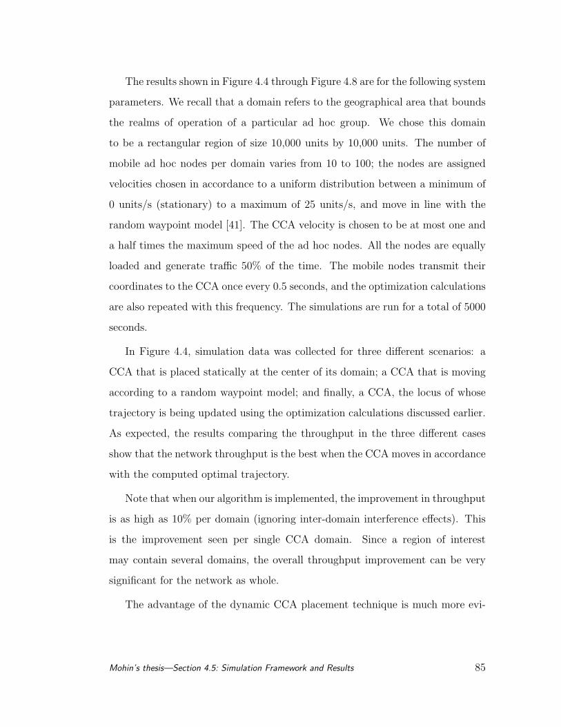
The results shown in Figure 4.4 through Figure 4.8 are for the following system

parameters. We recall that a domain refers to the geographical area that bounds

the realms of operation of a particular ad hoc group. We chose this domain

to be a rectangular region of size 10,000 units by 10,000 units. The number of

mobile ad hoc nodes per domain varies from 10 to 100; the nodes are assigned

velocities chosen in accordance to a uniform distribution between a minimum of

0 units/s (stationary) to a maximum of 25 units/s, and move in line with the

random waypoint model [41]. The CCA velocity is chosen to be at most one and

a half times the maximum speed of the ad hoc nodes. All the nodes are equally

loaded and generate traffic 50% of the time. The mobile nodes transmit their

coordinates to the CCA once every 0.5 seconds, and the optimization calculations

are also repeated with this frequency. The simulations are run for a total of 5000

seconds.

In Figure 4.4, simulation data was collected for three different scenarios: a

CCA that is placed statically at the center of its domain; a CCA that is moving

according to a random waypoint model; and finally, a CCA, the locus of whose

trajectory is being updated using the optimization calculations discussed earlier.

As expected, the results comparing the throughput in the three different cases

show that the network throughput is the best when the CCA moves in accordance

with the computed optimal trajectory.

Note that when our algorithm is implemented, the improvement in throughput

is as high as 10% per domain (ignoring inter-domain interference effects). This

is the improvement seen per single CCA domain. Since a region of interest

may contain several domains, the overall throughput improvement can be very

significant for the network as whole.

The advantage of the dynamic CCA placement technique is much more evi-


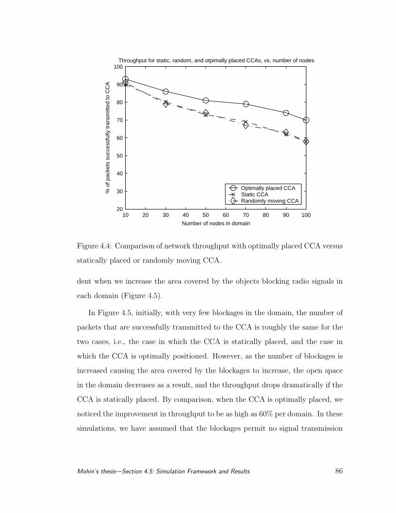
10 20 30 40 50 60 70 80 90 10020

30

40

50

60

70

80

90

100

Number of nodes in domain

% o

f pac

kets

suc

cess

fully

tran

smitt

ed to

CC

A

Throughput for static, random, and otpimally placed CCAs, vs. number of nodes

Optimally placed CCAStatic CCA Randomly moving CCA

Figure 4.4: Comparison of network throughput with optimally placed CCA versus

statically placed or randomly moving CCA.

dent when we increase the area covered by the objects blocking radio signals in

each domain (Figure 4.5).

In Figure 4.5, initially, with very few blockages in the domain, the number of

packets that are successfully transmitted to the CCA is roughly the same for the

two cases, i.e., the case in which the CCA is statically placed, and the case in

which the CCA is optimally positioned. However, as the number of blockages is

increased causing the area covered by the blockages to increase, the open space

in the domain decreases as a result, and the throughput drops dramatically if the

CCA is statically placed. By comparison, when the CCA is optimally placed, we

noticed the improvement in throughput to be as high as 60% per domain. In these

simulations, we have assumed that the blockages permit no signal transmission


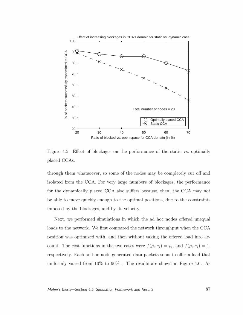
20 30 40 50 60 7020

30

40

50

60

70

80

90

100

Ratio of blocked vs. open space for CCA domain (in %)

% o

f pac

kets

suc

cess

fully

tran

smitt

ed to

CC

A

Effect of increasing blockages in CCA’s domain for static vs. dynamic case

Total number of nodes = 20

Optimally placed CCAStatic CCA

Figure 4.5: Effect of blockages on the performance of the static vs. optimally

placed CCAs.

through them whatsoever, so some of the nodes may be completely cut off and

isolated from the CCA. For very large numbers of blockages, the performance

for the dynamically placed CCA also suffers because, then, the CCA may not

be able to move quickly enough to the optimal positions, due to the constraints

imposed by the blockages, and by its velocity.

Next, we performed simulations in which the ad hoc nodes offered unequal

loads to the network. We first compared the network throughput when the CCA

position was optimized with, and then without taking the offered load into ac-

count. The cost functions in the two cases were f(ρi, τi) = ρi, and f(ρi, τi) = 1,

respectively. Each ad hoc node generated data packets so as to offer a load that

uniformly varied from 10% to 90% . The results are shown in Figure 4.6. As


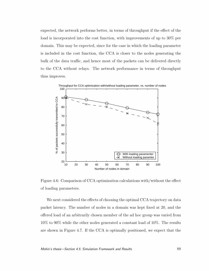
expected, the network performs better, in terms of throughput if the effect of the

load is incorporated into the cost function, with improvements of up to 30% per

domain. This may be expected, since for the case in which the loading parameter

is included in the cost function, the CCA is closer to the nodes generating the

bulk of the data traffic, and hence most of the packets can be delivered directly

to the CCA without relays. The network performance in terms of throughput

thus improves.

10 20 30 40 50 60 70 80 90 10020

30

40

50

60

70

80

90

100

Number of nodes in domain

% o

f pac

kets

suc

cess

fully

tran

smitt

ed to

CC

A

Throughput for CCA optimization with/without loading parameter, vs. number of nodes

With loading paramenter Without loading paramter

Figure 4.6: Comparison of CCA optimization calculations with/without the effect

of loading parameters.

We next considered the effects of choosing the optimal CCA trajectory on data

packet latency. The number of nodes in a domain was kept fixed at 20, and the

offered load of an arbitrarily chosen member of the ad hoc group was varied from

10% to 90% while the other nodes generated a constant load of 10%. The results

are shown in Figure 4.7. If the CCA is optimally positioned, we expect that the


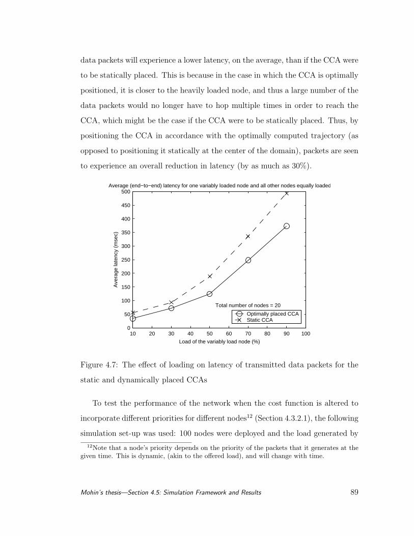
data packets will experience a lower latency, on the average, than if the CCA were

to be statically placed. This is because in the case in which the CCA is optimally

positioned, it is closer to the heavily loaded node, and thus a large number of the

data packets would no longer have to hop multiple times in order to reach the

CCA, which might be the case if the CCA were to be statically placed. Thus, by

positioning the CCA in accordance with the optimally computed trajectory (as

opposed to positioning it statically at the center of the domain), packets are seen

to experience an overall reduction in latency (by as much as 30%).

10 20 30 40 50 60 70 80 90 1000

50

100

150

200

250

300

350

400

450

500

Load of the variably load node (%)

Ave

rage

late

ncy

(mse

c)

Average (end−to−end) latency for one variably loaded node and all other nodes equally loaded

Total number of nodes = 20

Optimally placed CCAStatic CCA

Figure 4.7: The effect of loading on latency of transmitted data packets for the

static and dynamically placed CCAs

To test the performance of the network when the cost function is altered to

incorporate different priorities for different nodes12 (Section 4.3.2.1), the following

simulation set-up was used: 100 nodes were deployed and the load generated by

12Note that a node’s priority depends on the priority of the packets that it generates at thegiven time. This is dynamic, (akin to the offered load), and will change with time.


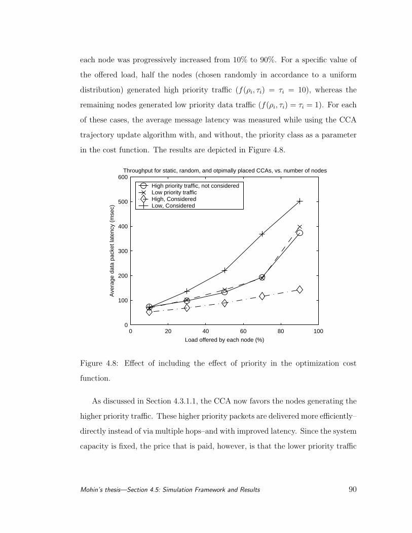
each node was progressively increased from 10% to 90%. For a specific value of

the offered load, half the nodes (chosen randomly in accordance to a uniform

distribution) generated high priority traffic (f(ρi, τi) = τi = 10), whereas the

remaining nodes generated low priority data traffic (f(ρi, τi) = τi = 1). For each

of these cases, the average message latency was measured while using the CCA

trajectory update algorithm with, and without, the priority class as a parameter

in the cost function. The results are depicted in Figure 4.8.

0 20 40 60 80 1000

100

200

300

400

500

600

Load offered by each node (%)

Ave

rage

dat

a pa

cket

late

ncy

(mse

c)

Throughput for static, random, and otpimally placed CCAs, vs. number of nodes

High priority traffic, not considered Low priority traffic High, Considered Low, Considered

Figure 4.8: Effect of including the effect of priority in the optimization cost

function.

As discussed in Section 4.3.1.1, the CCA now favors the nodes generating the

higher priority traffic. These higher priority packets are delivered more efficiently–

directly instead of via multiple hops–and with improved latency. Since the system

capacity is fixed, the price that is paid, however, is that the lower priority traffic


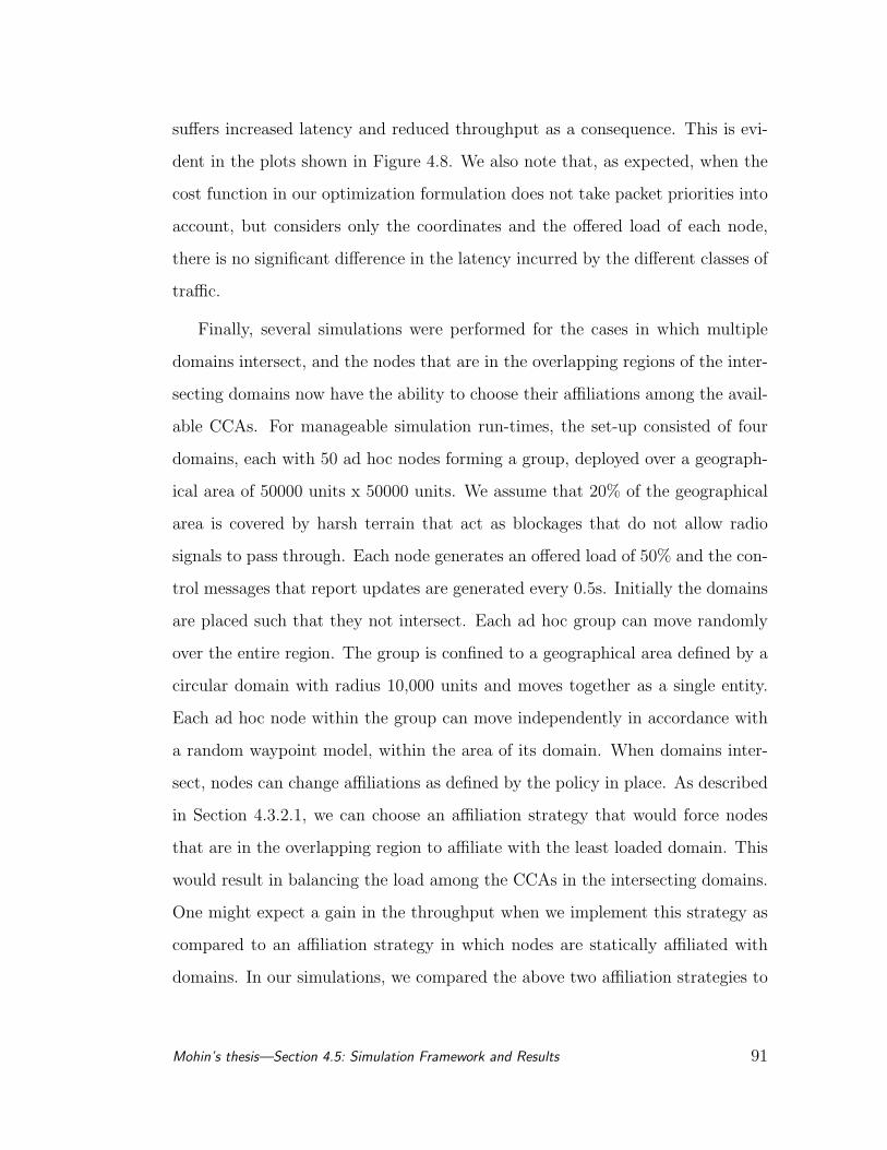
suffers increased latency and reduced throughput as a consequence. This is evi-

dent in the plots shown in Figure 4.8. We also note that, as expected, when the

cost function in our optimization formulation does not take packet priorities into

account, but considers only the coordinates and the offered load of each node,

there is no significant difference in the latency incurred by the different classes of

traffic.

Finally, several simulations were performed for the cases in which multiple

domains intersect, and the nodes that are in the overlapping regions of the inter-

secting domains now have the ability to choose their affiliations among the avail-

able CCAs. For manageable simulation run-times, the set-up consisted of four

domains, each with 50 ad hoc nodes forming a group, deployed over a geograph-

ical area of 50000 units x 50000 units. We assume that 20% of the geographical

area is covered by harsh terrain that act as blockages that do not allow radio

signals to pass through. Each node generates an offered load of 50% and the con-

trol messages that report updates are generated every 0.5s. Initially the domains

are placed such that they not intersect. Each ad hoc group can move randomly

over the entire region. The group is confined to a geographical area defined by a

circular domain with radius 10,000 units and moves together as a single entity.

Each ad hoc node within the group can move independently in accordance with

a random waypoint model, within the area of its domain. When domains inter-

sect, nodes can change affiliations as defined by the policy in place. As described

in Section 4.3.2.1, we can choose an affiliation strategy that would force nodes

that are in the overlapping region to affiliate with the least loaded domain. This

would result in balancing the load among the CCAs in the intersecting domains.

One might expect a gain in the throughput when we implement this strategy as

compared to an affiliation strategy in which nodes are statically affiliated with

domains. In our simulations, we compared the above two affiliation strategies to


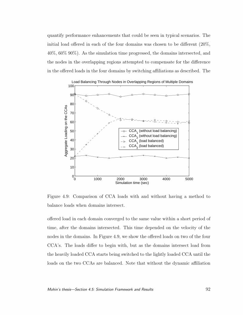
quantify performance enhancements that could be seen in typical scenarios. The

initial load offered in each of the four domains was chosen to be different (20%,

40%, 60% 90%). As the simulation time progressed, the domains intersected, and

the nodes in the overlapping regions attempted to compensate for the difference

in the offered loads in the four domains by switching affiliations as described. The

0 1000 2000 3000 4000 50000

10

20

30

40

50

60

70

80

90

100

Simulation time (sec)

Agg

rega

te L

oadi

ng o

n th

e C

CA

s

Load Balancing Through Nodes in Overlapping Regions of Multiple Domains

CCA1 (without load balancing)

CCA2 (without load balancing)

CCA1 (load balanced)

CCA2 (load balanced)

Figure 4.9: Comparison of CCA loads with and without having a method to

balance loads when domains intersect.

offered load in each domain converged to the same value within a short period of

time, after the domains intersected. This time depended on the velocity of the

nodes in the domains. In Figure 4.9, we show the offered loads on two of the four

CCA’s. The loads differ to begin with, but as the domains intersect load from

the heavily loaded CCA starts being switched to the lightly loaded CCA until the

loads on the two CCAs are balanced. Note that without the dynamic affiliation


strategy, the loads in each domain remain static, and equal to the offered load at

the initiation of the simulation.

4.6 Conclusions

In order to support scalability in ad hoc networks, one can envision the deploy-

ment of a range extension network that consists of airborne nodes, satellites,

power transmission towers and such. In order to interface the ad hoc network

with the range extension network, one approach could be to deploy gateways that

we refer to as CCAs to relay data traffic from/to an ad hoc group to/from the

range extension network. This is akin to providing a centralized infrastructure

within the infrastructure-less ad hoc network. The objective of this work is to

determine where the CCA is to be placed relative to the ad hoc group of nodes

such that certain network performance metrics are optimized. This objective can

be formulated as a set of convex optimization problems. By means of suitable

modifications, we simplify these convex formulations such that they can be very

efficiently solved by numerical methods.

We evaluate the improvements in network performance that we achieve by

means of extensive simulations, where the CCA is enforced to follow the com-

puted optimal trajectory. Simulation results indicate that the network through-

put improves by about 10-15% per CCA domain13 (an ad hoc domain consisting

of about 50 nodes), if the CCA moves in accordance with the optimally computed

trajectory as opposed to being static or moving in accordance to a random way-

point model. A similar improvement is seen in terms of a reduction in latency

that the data packets experience. The cost function in our optimization formu-

13The overall improvement would be several multiples of this value, since a region of interestwill likely contain several CCA domains.

Mohin’s thesis—Section 4.6: Conclusions 93

lation can also be appropriately modified to support better performance for high

priority traffic, as compared to the performance for lower priority traffic. We also

consider cases wherein the nodes have the ability to choose different CCAs for

relaying their inter-domain traffic and show that this ability can be exploited to

balance the loads in different domains, thereby improving performance further.

We also show that the operations that are required in order to thus define an

optimal trajectory for the mobile CCAs, can be performed efficiently and quickly

by most commercial, off-the-shelf micro-processors, and with little additional

overhead.

One particular extension of interest, is to incorporate fault tolerance in our

composite ad hoc network, since the CCA is a catastrophic single point of failure.

In this scenario, we can envision multiple nodes in a domain, each of which is

capable of acting as the CCA. In that case, should the primary CCA fail, then,

according to some pre-determined rule, one of these dormant CCAs can take over

as the new CCA. This issue is investigated in detail in Section 5.4 in Chapter 5,

under the more broad context of dependability of hybrid networks.

Mohin’s thesis—Section 4.6: Conclusions 94

CHAPTER 5

Dependability of Wireless Heterogeneous

Networks

As we have seen in Chapters 3 and 4, a sensor network—and by extension, ad hoc

networks—can be very general, involving heterogeneous collections of several net-

works including: wireless ground ad hoc nodes, airborne nodes, low earth orbiting

and geostationary nodes, access portals to the wired infrastructure, or gateways

to other hybrid networks. The challenge is to enable and maintain connectivity

between all the disparate components, and to serve the communication needs of

the client nodes in the best manner possible. We outlined a detailed architecture

in Chapter ****** as one possible technique for accomplishing this objective—by

using gateway nodes as inter-domain communication portals. However, it was

seen that such gateway-based architectures then resemble a hierarchical struc-

ture for information flow, as discussed earlier in Section 2.4.1 (Figure 2.9). This

causes the network to have single points of failures, and thus decreases the overall

reliability of the entire network1.

In this chapter, these issues are explored for general heterogeneous networks.

As discussed in Chapter 2, peer-to-peer, decentralized architectures offer flexibil-

ity and diversity for of data fusion and information flow, as opposed to centralized

or hierarchical architectures. As we will see in this chapter, an additional impor-

1Some mitigating techniques involving redundant gateways and associated protocols arediscussed in detail later in this chapter, in Section 5.4

95

tant benefit is increased reliability and survivability—terms that will be precisely

defined in the sequel. However, these benefits all come at the price of increased

network administration cost and complexity. One of the goals of this chapter will

be to analyze and develop novel techniques that will allow us to optimize the reli-

ability of networks for efficient information processing, subject to the complexity

and overhead costs.

5.1 Introduction

Although significant work has been done in the context of wireline networks for

improving system reliability, availability and survivability (e.g. for the public

switched telephone network), very little work has been done for infrastructure

based wireless networks (e.g. the cellular and PCS networks [92]), and for ad

hoc networks (e.g. IEEE802.11 or Bluetooth based systems [85, 105]). With

the enormous interest in the development of such infrastructure-less communi-

cation devices in recent times, both in the commercial and military world, it is

imperative to investigate and understand well the statistical reliability and de-

pendability of such systems. The focus of this chapter is the development of

analysis and design tools to enhance the dependability of peer-to-peer wireless

networks. The goal is to design a secure and adaptive networking and communi-

cation infrastructure for a system of hybrid wireless sensor nodes or general ad

hoc networks.

We first introduce some terminology from the network reliability discipline.

For both wireline and wireless networks, the current consensus for measuring

the ability of a network to avoid or cope with a failure is by means of three

inter-related parameters, as defined below.


Definiton 5.1. The reliability of a network is its ability to perform a designated

set of functions for a specified operational lifetime, under a given set of conditions.

Definiton 5.2. The availability of a network is its ability to perform a designated

set of functions at any given instant, under a given set of conditions. Average

availability is thus a function of how often something fails and how long it takes

to recover from a failure.

Definiton 5.3. The survivability of a network is its ability to perform a desig-

nated set of functions, given a set of network infrastructure failures resulting in

service outage. The outage can, in general, be described by the number of ser-

vices affected, the number of subscribers affected, and the duration of the outage,

for a specified set of conditions.

The reliability, availability and survivability of a network is collective referred

to as the dependability of the network. A heterogeneous peer-to-peer wireless

network can be considered as a ‘complex system’, where the various parts of the

system give rise to the collective behaviors of the system [46]. In such cases,

the performance and reliability of the system as a whole are influenced by, and

intertwined with, subtle and often indirect effects of the individual components.

Our goal is to build a platform for the analysis of these problems in a systematic

fashion. As mentioned earlier, a great deal of research has already been done

in the related fields of hardware/software fault tolerance, statistical reliability

analysis of systems, probabilistic analysis of complex systems, graph theory, etc.

[50, 82]. Our aim is to build on these foundations by identifying and appropriately

modifying the key techniques from this vast body of knowledge that will enable

analysis or yield insight for the case of heterogeneous ad hoc networks.

Several issues make this problem considerably complex. These are: general

ad hoc networks can be mobile, with dynamic performance parameters having no


long run equilibrium conditions; they may have distributed feedback effects which

may be both intended or unintended; they may be primarily ‘agent-based’ where

the agents, e.g. fusion nodes (Chapter 2) or gateway nodes (Chapter ******) act

locally within some sort of group or hierarchy, but often in contention with other

groups of agents engaged in similar actions (a sort of fractal organization at a

coarse level).

The basic question of reliability of such systems is notoriously hard to quantify

or analyze, for the simple reason that the reliability of the individual components

do not always indicate the reliability for the system as a whole. However, it is

unequivocal that the network infrastructure has to be reliable and fault tolerant.

Its performance has to degrade gracefully in the face of different type of failures

(e.g. progressive, cascading, catastrophic, malicious attacks, or probabilistic),

and failure-recovery mechanisms have to be robust and efficient.

The standard approach is to first formalize the relevant concepts from complex

systems by: 1) understanding the ways of modeling and describing the complex

system, 2) mapping the interactions of the heterogeneous components that in

turn give rise to patterns of behavior, and 3) analyzing the process of formation

of complex systems through pattern formation and evolution.

For reliability modeling of multi-tiered networks, we show in the subsequent

sections that this is essentially equivalent to characterizing the connectivity prop-

erties of the network in an abstract fashion. We rely on the mature mathematical

discipline of graph theory to provide a comprehensive foundation. Furthermore,

statistics can be obtained for the individual node and link failure probabilities

(or estimated from the protocols themselves by inferential or Monte Carlo tech-

niques), and standard statistical and estimation techniques can then be used to

derive connectivity estimates, within confidence-interval limits. This is an ex-


perimental task that this chapter does not address explicitly; rather we assume

that this data is available for the final step, which is the design of algorithms to

maximize the reliability of the network, given system constraints, as discussed in

subsequent sections.

With regards to mapping the interactions of the heterogeneous components

(e.g. gateways and nodes that it serves), we have modified standard reliability

results from the cellular and wire-line networks to apply to the ad hoc case. The

mobility and dynamic nature of the ad hoc network itself can then be averaged as

a sort of outer integration akin to E(X) expectation calculations in probability

science, subject to estimating motion and terrain statistics, and we can thus

obtain figures for reliability of the network as a whole, (as experienced by an

‘average’ node in the network).

Finally, as these complex systems evolve with the addition/removal of net-

work elements, the effects on overall system reliability depend on being able to

modularize the reliability computations as much as possible to the level of the dif-

ferent sub-networks, and to derive their inter-relationships. Unfortunately, most

graph theory problems of this type have been shown to be NP-hard problems

[40]. Therefore, the usual recourse is to employ approximations and asymptotic

analysis techniques for bounding the results, as illustrated for the case of delay

in random wireless networks in Section 3.2.1.

5.2 Graph Theory Fundamentals for Modeling Ad Hoc

Networks

In this preliminary section, we focus on the task of modeling ad hoc networks

for the purpose of dependability analysis. This is essentially equivalent to char-

Mohin’s thesis—Section 5.2: Graph Theory Fundamentals for

Modeling Ad Hoc Networks 99

acterizing the connectivity properties of the network in an abstract fashion. For-

tunately, we can rely on the mature mathematical discipline of graph theory to

accomplish this task [100]. The basic idea is to formulate some appropriate reli-

ability measures to which we can then apply current graph-theoretic techniques.

5.2.1 Deterministic Graphs

A static network of wireless or wired communication nodes (e.g. static sensor

networks) can be modeled as a deterministic directed graph [100]. The nodes of

the graph can correspond to the transmitting or receiving units, and the edges of

the graph would correspond to the connections that link the nodes in the network

and describe its network topology/architecture. With this simple model, we can

obtain estimates of the average connectivity properties of the network, and thus

bound the reliability metrics of interest. However, since general ad hoc networks

can be mobile, this basic deterministic graph model is insufficient to capture the

effects of mobility on the topology of the network. Instead, this is accomplished

by considering the mobile wireless ad hoc network as a random graph, where

the links state (as well as the node states) at particular instants of time have

probability distributions (Section 5.2.2). Some terminology is introduced first.

Definiton 5.4. A graph is defined algebraically as a collection, G(V, E), of two

sets:

• V (G), E(G), where V = V (G) is the set of p > 1 nodes or vertices of the

graph;

• E = E(G) is a set of q ≥ 0 pairs of nodes.

We say that G has order p and size q and refer to G as a (p, q) graph. The

elements of E are the edges, or links of G, and edge e = (u, v) is said to join



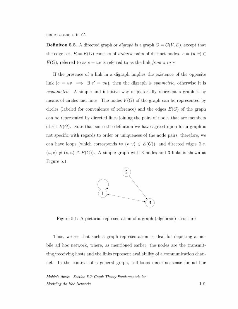
nodes u and v in G.

Definiton 5.5. A directed graph or digraph is a graph G = G(V, E), except that

the edge set, E = E(G) consists of ordered pairs of distinct nodes. e = (u, v) ∈E(G), referred to as e = uv is referred to as the link from u to v.

If the presence of a link in a digraph implies the existence of the opposite

link (e = uv =⇒ ∃ e′ = vu), then the digraph is symmetric, otherwise it is

asymmetric. A simple and intuitive way of pictorially represent a graph is by

means of circles and lines. The nodes V (G) of the graph can be represented by

circles (labeled for convenience of reference) and the edges E(G) of the graph

can be represented by directed lines joining the pairs of nodes that are members

of set E(G). Note that since the definition we have agreed upon for a graph is

not specific with regards to order or uniqueness of the node pairs, therefore, we

can have loops (which corresponds to (v, v) ∈ E(G)), and directed edges (i.e.

(u, v) 6= (v, u) ∈ E(G)). A simple graph with 3 nodes and 3 links is shown as

Figure 5.1.

Figure 5.1: A pictorial representation of a graph (algebraic) structure

Thus, we see that such a graph representation is ideal for depicting a mo-

bile ad hoc network, where, as mentioned earlier, the nodes are the transmit-

ting/receiving hosts and the links represent availability of a communication chan-

nel. In the context of a general graph, self-loops make no sense for ad hoc



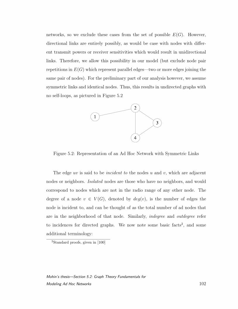
networks, so we exclude these cases from the set of possible E(G). However,

directional links are entirely possibly, as would be case with nodes with differ-

ent transmit powers or receiver sensitivities which would result in unidirectional

links. Therefore, we allow this possibility in our model (but exclude node pair

repetitions in E(G) which represent parallel edges—two or more edges joining the

same pair of nodes). For the preliminary part of our analysis however, we assume

symmetric links and identical nodes. Thus, this results in undirected graphs with

no self-loops, as pictured in Figure 5.2

Figure 5.2: Representation of an Ad Hoc Network with Symmetric Links

The edge uv is said to be incident to the nodes u and v, which are adjacent

nodes or neighbors. Isolated nodes are those who have no neighbors, and would

correspond to nodes which are not in the radio range of any other node. The

degree of a node v ∈ V (G), denoted by deg(v), is the number of edges the

node is incident to, and can be thought of as the total number of ad nodes that

are in the neighborhood of that node. Similarly, indegree and outdegree refer

to incidences for directed graphs. We now note some basic facts2, and some

additional terminology:

2Standard proofs, given in [100]



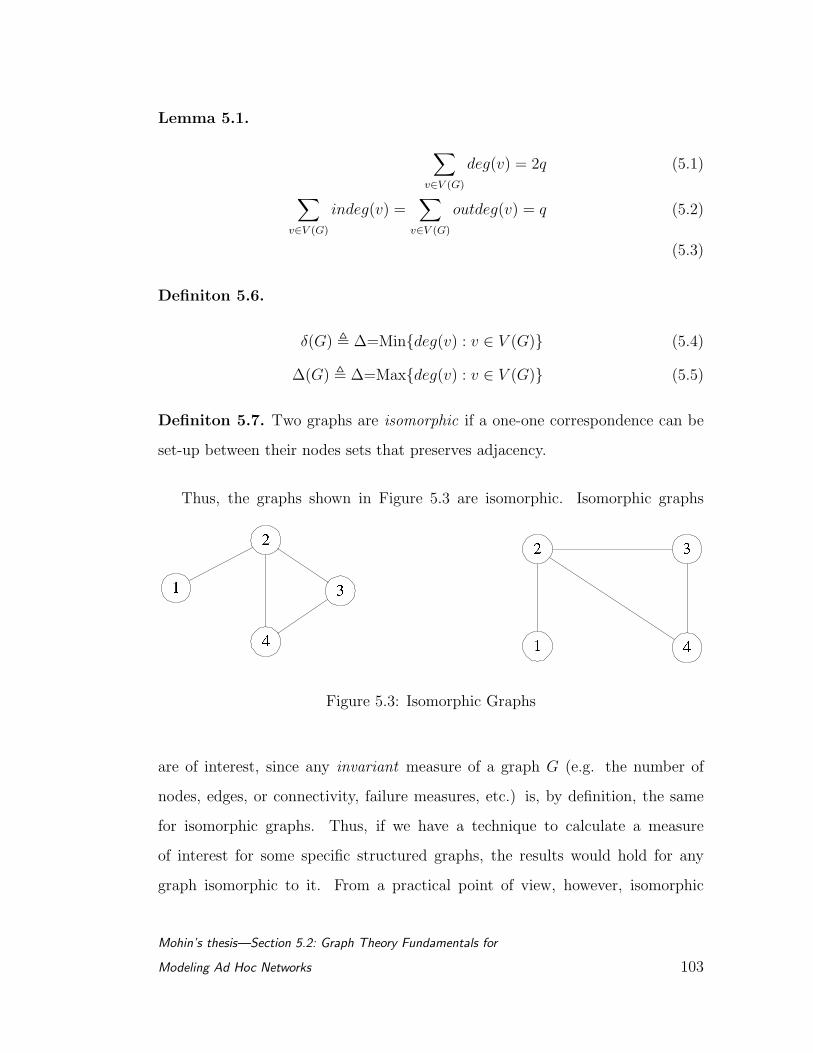
Lemma 5.1.

∑

v∈V (G)

deg(v) = 2q (5.1)

∑

v∈V (G)

indeg(v) =∑

v∈V (G)

outdeg(v) = q (5.2)

(5.3)

Definiton 5.6.

δ(G) , ∆=Mindeg(v) : v ∈ V (G) (5.4)

∆(G) , ∆=Maxdeg(v) : v ∈ V (G) (5.5)

Definiton 5.7. Two graphs are isomorphic if a one-one correspondence can be

set-up between their nodes sets that preserves adjacency.

Thus, the graphs shown in Figure 5.3 are isomorphic. Isomorphic graphs

Figure 5.3: Isomorphic Graphs

are of interest, since any invariant measure of a graph G (e.g. the number of

nodes, edges, or connectivity, failure measures, etc.) is, by definition, the same

for isomorphic graphs. Thus, if we have a technique to calculate a measure

of interest for some specific structured graphs, the results would hold for any

graph isomorphic to it. From a practical point of view, however, isomorphic



graphs would actually represent different physical arrangements of the nodes in a

particular domain, but with the same connectivity properties. Thus, isomorphism

allows us to reduce the cardinality of the infinite set of possible geographical

locations of the nodes.

Definiton 5.8. A weighted graph is graph a G = G(V,E) together with a weight

function w : E(G) 7→ R where w(e) is the weight assigned to the edge e ∈ E(G).

In applications, this might represent the cost, reliability, or capacity of a

communication channel in a radio network. It is also possible to consider graphs

with weights assigned to the nodes v ∈ V (G), representing the costs associated

with storage locations, power consumption, or CPU capacity of nodes in a data

network. In this manner, a cost function can be built for evaluating metrics

such as routing or MAC as a function of link/node formation and breakage. Our

main interest will eventually be in communication networks given by a symmetric

(i.e. bi-directional capable), or asymmetric (i.e. uni-directional capable) digraph

with a weight function P : E(G) 7→ [0, 1]. Here P (e) represents the probability

that the communication link e ∈ E(G) is operational, on a bit, packet, or frame

level. Ideally, this probability is allowed to depend on the direction of the link in

order to model such things as local jamming, directional antennas for transmission

and/or reception, etc.

We next discuss some connectivity concepts that correspond directly to con-

nectivity in multi-hop ad hoc networks. A walk in a graph G is an alternating

sequence of nodes and edges, e.g. v0, e1, v1, e2 . . . , vn. It is said to connect nodes

v1 and vn and has length n. A walk is closed if v0 = vn, otherwise it is open; it

is a trail if its edges are distinct, and it is a path if its nodes (and hence also its

edges) are distinct. A circuit is a closed path and a cycle is a circuit with distinct

nodes (other than the initial node v0 = vn). Two nodes u, , v ∈ G are said to be



connected if there is a path from u to v, and the graph is said to be connected

graph if every pair of nodes is so connected.

Thus, we can see that graph connectivity is a fairly exact analogue of the

concept behind connectivity in an ad hoc network. What is of paramount interest,

however, is some measures by which connectivity can be quantified. The usual

way to do this is to specify the number of nodes or edges that must be removed

in order to disconnect G.

Definiton 5.9. A graph G is n-connected, n ≥ 1 if it remains connected after the

removal of any set of n − 1 vertices. The node-connectivity κ(G) is the smallest

number of vertices whose removal results in a disconnected graph.

Similarly, an n-edge connected graph and the edge-connectivity, λ(G), can be

defined.

Lemma 5.2.

κ(G) ≤ λ(G) ≤ δ(G) (5.6)

For the design of reliable communication networks, it is important to ensure

large values of κ(G) and λ(G), since this provides for many alterative paths for

communication between nodes. Conversely, small values of these graph invariants

imply that the network is relatively vulnerable and can be disabled (i.e. discon-

nected) by the removal of only a few of its nodes or links. Statistically, for ad

hoc networks, it is usually the case that edge failures are far more common than

node failures.

We conclude this brief section on graph theory fundamentals by highlighting

some classical results in graph connectivity (see [100] for proofs).

Lemma 5.3. For a graph G with p nodes and q edges:



1. If q < p− 1 then G is disconnected

2. If q > frac(p− 1)(p− 2)2, then G is connected

3. If δG ≥ p/2 then λ(G) = δ(G)

4. If δ(G) > frac(p + n− 2)2, where 1 ≤ n < p, then G is n-connected.

Theorem 5.1 (Menger’s Theorems). —Node/Edge Version

1. κ(G) ≥ n iff for each pair u, v ∈ V (G) of distinct, non-adjacent nodes, there

exist at least n node-disjoint paths which connect u and v.

2. λ(G) ≥ n iff for each pair u, v ∈ V (G) of distinct nodes there exist at least

n edge-disjoint paths which connect u and v.

5.2.2 Probabilistic Graphs and Reliability Measures

We have seen in the previous subsection that a static ad hoc network, such as

a sensor network, can be modeled as a deterministic algebraic graph structure.

A mobile wireless ad hoc network, on the other hand, can be modeled as a ran-

dom graph where the nodes of the graph correspond to transmitting or receiving

mobile units, and the edges of the graph correspond to the connection state of

the network at a particular instant in time. Furthermore, for the links in the

network represented by the dynamic edges in the graph, a weighting function,

p : E(G) 7→ R, can be defined. This can be used to represent a variety of link-

dependent parameters for the ad hoc network, e.g. the capacity of the link, or

the failure probability, etc. We are particularly interested in the case where the

weighting function, P1 : E(G) 7→ [0, 1], represents the probability of an edge

being operational. Similarly, another weighting function, P2 : V (G) 7→ [0, 1] can

be defined for nodes, which represents the probability of a node itself being oper-



ational. The determination of these functions is system dependent (the physical

layer coding being used, network layer protocols being used, geographical terrain

of operation, etc.), and is a major area of research that is not the focus of this

section. It is assumed that these estimates are obtained by the reliability proto-

cols from lower layer protocols in the network. Numerical issues are discussed,

however, in the sections below.

With these metrics, we can consider some ‘common sense’ notions of reli-

ability. For example, for a given source node in the ad hoc network, and a

corresponding target or destination node, one may ask what is the chance of

reliably sending packets from source to target? The myriad protocols for the 7

layer OSI stack are all designed to accomplish the actual connectivity and packet

transfer tasks, but by themselves they cannot provide performance bounds when

this question is asked from the perspective of a heterogeneous ad hoc network as

an end-to-end system3. This is illustrative of the complex systems analogy given

earlier, where the individual protocols at each layer of the network stack for each

node in the network (involved in the transfer process) are working hard to ensure

reliable and error free operation, but in so doing are interacting with each other

in uncertain ways. As a result, the reliability of the entire process cannot be

derived simply from the reliability of any particular protocol layer.

Instead, we note that we can quite naturally abstract the problem and define

a probabilistic notion of connectivity to answer the reliability question. Thus, if

we can gather the statistics for the individual node and link failure probabilities

(or obtain this data from the protocols themselves by inferential or Monte Carlo

techniques), then we can apply standard statistical and estimation techniques

to obtain connectivity estimates, within confidence-interval limits. This is the

3except in some special cases of the grid, star, etc. networks.



essence of statistical dependability analysis as applied to ad hoc network con-

nectivity [101]. The mobility and dynamic nature of the ad hoc network itself

can then be averaged as a sort of outer integration akin to E(X) expectation

calculations, subject to estimating motion and terrain statistics, and we can thus

obtain figures for dependability of the network as a whole, as experienced by an

‘average’ node in the network. A similar approach was taken to estimate the

order of the delay in random wireless networks, as shown in Section 3.2.1.

The most common statistic used in the technical literature for the reliability

of wired networks is the K-terminal reliability [13].

Definiton 5.10. If K ⊂ V (G) is a subset of the nodes, and the K-terminal

reliability is the probability that every two vertices in K are connected by a path

of operational edges.

In an ad hoc network, we are more interested in a single source-destination

pair, known as st-reliability, in which case |K| = 2, or in the all-terminal relia-

bility, for which K = V (G). The former is denoted in the technical literature as

Rel(G; s, t). For an undirected graph, the st-reliability is a special case of that

for a directed graph (since each edge is then equivalent to two edges with oppo-

site directions but equal probability of success). In that case, the st-reliability is

simply the probability that the network is connected, or that G contains at least

one operational spanning tree or subgraph. This is a useful measure for any ad

hoc network, since it indicates the likelihood of a transmitted package to reach a

desired destination from the source.

The subtle thing to note here is that the st-reliability metric does not measure

the probability along a specific route that a particular routing/MAC algorithm

has discovered, or looked up in a table. Rather, it measures the possibility that

any operational path can be found by the underlying algorithms. This is a more



accurate measure of the network performance, as experienced the data packets

in the network. To generalize for a global ‘average’ for the network as a whole,

another common metric is the following.

Definiton 5.11. The resiliency of a network is the st-reliability averaged over

all p(p− 1) possible node pairs:

Res(G) =1

p(p− 1)

∑

s,t∈V (G)

Rel(G; s, t) (5.7)

Thus far the emphasis has been on link failures. An important metric can

now be defined for node failures in networks, which characterize the vulnerability

(Section 5.1) of a network. To capture the concept of network vulnerability

(e.g. in the face of hostile attacks or cascade failures of nodes), a concept from

the wired networks discipline can be extended to the heterogeneous wireless case.

Definiton 5.12. The Node-connectivity factor (NCF) represents the average

number of nodes that have to be removed from a network in order for the remain-

ing subgraph to be totally disconnected. This quantity can be defined recursively,

since if G is disconnected and has components G1, G2, . . . , Gm, then:

NCF(G) , ∆=m∑

i=1

NCF(Gi) (5.8)

For a connected graph G, if κ(g) is the size of the smallest set Vo ⊂ V (G) for

which G− V0 is disconnected, and if χ1, . . . , χn is the collection of all such node

sets V0, then:

NCF(G) , κ(G) +1

n

∑i=1

nNCF(G− χi) (5.9)

The NCF and a similarly defined quantity for links—the link-connectivity factor

(LCF)— are useful indicators of the relative advantage of one particular resource

allocation scheme in a network versus another, and thus aids in optimizing net-

work dependability. In Section 5.3.1, this parameter is used in defining one such



novel optimization protocol for heterogeneous wireless networks. Finally, we con-

sider the diameter of a graph:

Definiton 5.13. The diameter of a graph G is the maximum hop distance sup-

ported by the edge configuration:

Diam(G) = maxdist(u, v) : u, v ∈ V (G) (5.10)

Recently, this metric has been preferred for quantifying forms of the quality

of service (QoS) for networks, and is of considerable interest in the context of

hybrid ad hoc networks. The basic idea is once again simple: a graph with

a small expected diameter is better-connected than one with a large expected

diameter.

5.3 Dependability Optimization for Node Failures

We have thus far developed an analytic and optimization framework for investi-

gating the dependability of hybrid ad hoc networks in the face of link failures. In

this section, we treat the problem of node failures, and propose a relatively simple

network design scheme for optimizing reliability in networks with the possibility

of node failures.

Statistically, in mobile ad hoc networks, link failures are orders of magnitude

more probable that node failures, because of mobility-induced dynamic topology

changes in the network. Thus, optimal network design focusing on routing and

MAC techniques for handling link failures are more commonly used than node

failure protocols. However, being able to handle node failures is of paramount

importance in some specific architectures. For example, in the case study pre-

sented in Section 5.4, the NGI architecture involving gateways in heterogeneous

Mohin’s thesis—Section 5.3: Dependability Optimization for Node

Failures 110

hybrid ad hoc networks is studied. We observed earlier in Chapter 4 that gate-

ways are single points of catastrophic failures for such multi-tiered networks. In

this regard, we present distributed, fault tolerant techniques for handling such

node failures—primarily by relying on redundancy in the network. A similar

situation applies for the case of static sensor networks performing data fusion at

centralized or hierarchical nodes (Section 2.2.4).

Single points of failures are a characteristic shortcoming of all hierarchical

networks, as discussed at the outset in Section 2.4.1. This is the reason for pre-

ferring ad hoc network architectures in NGI networks. We have determined that

most of the existing survivability measures that have been reported are inade-

quate for applying to hybrid networks since the Internet-centric hybrid wireless

networks of today are subject to deliberate and/or random attacks [101]. Since

the destruction of a network is essentially a process in which the nodes of the

network are gradually destroyed until completely disconnected, a dependability

measure should be based upon such a process and its definition should reflect

the survivability of the network during the entire destruction process. We now

propose a dependability measure for hybrid networks to quantify and optimize

node failure survivability.

5.3.1 Distributed Node Resilience Criteria (DNRC) for Peer-to-Peer

Networks

There have been many measures proposed for the dependability analysis of node

(and link) failures in networks [75]. Most of the techniques are based on graph the-

ory metrics, and primarily on minimum-cut tree enumeration techniques. How-

ever, these methods generally yield complicated computations, except for well

known network structures such as grid or star networks. Especially for the case


Failures 111

of mobile networks, the computation time (and network overhead) required often

makes minimum-cut tree calculations moot, since the topology will have changed

by the time the dependability results become available for network optimization.

To mitigate this undesirable situation, we now develop a new measure of de-

pendability for hybrid networks. This is based upon the estimation of the network

connectivity in a complete destruction process, i. e. the network connectivity is

summed with the node of the network being removed one by one until the network

becomes disconnected.

Definiton 5.14. For a network G with n nodes, the Distributed Node Resilience

Criteria (DNRC), denoted by γ, is defined as:

γ(G) =m−1∑

k=0

ξ(k) (5.11)

where ξ(k) is the connectivity measure of network Gk, which is produced by

removing the most important node from the network Gk−1 for k = 1, 2, . . . , m−1,

and m is the number of nodes which have to be removed before the network

becomes totally disconnected. Thus, ξ(0) measures the connectivity of the whole

network G, and ξ(k) is given by:

ξ(k) =n−k−1∑

i=1

n−k∑j=i+1

NCFk(i, j) (5.12)

Here NCFk(i, j) is the node connectivity factor, as defined earlier in Equation

(5.9), between i and j in the network Gk, and n − k is the number of nodes in

the network Gk. NCFk(i, j) can be simplified in this case to:

NCFk(i, j) =x∑

r=1

1

µ(r)(5.13)

where r is the number of independent paths between nodes i and j and µ(r) is

the number of hops long the rth independent path between nodes i and j.


Failures 112

Definiton 5.15. The priority factor of node i, denoted by PF(i), is the number

of all independent paths that include the node i in the network Gk, for i =

1, . . . , (n− k).

Since our objective in introducing the DNRC measure is to reduce the compli-

cations inherent in computing standard dependability metrics, we assume some

plausible node failure characteristics to keep the calculations relatively tractable.

These are:

• The nodes are considered to be either operational or non-operational. This

removes the necessity of using complex queuing theory models to account

for partially operational nodes via Markovian statistics.

• Only a single node is rendered inactive at any instant of time. This elim-

inates the case of multiple nodes being damaged simultaneously (which

is nonetheless possible in tactical deployments of dense sensor networks,

e.g., where a group of nodes are targeted for destruction). Without this

constraint, the analysis becomes significantly involved, since the network

architecture then changes drastically.

• Link failures are not considered in the optimization calculations. This met-

ric is explicitly geared to handle node failures; link failure optimization

techniques are assumed to be dealt with the underlying routing/MAC pro-

tocol for the wireless network.

An example calculation is illustrated next. Consider the network as pictured

in Figure 5.4, for graphs (i)G and (ii)G1 In the network G, Figure 5.4(i), we can


Failures 113

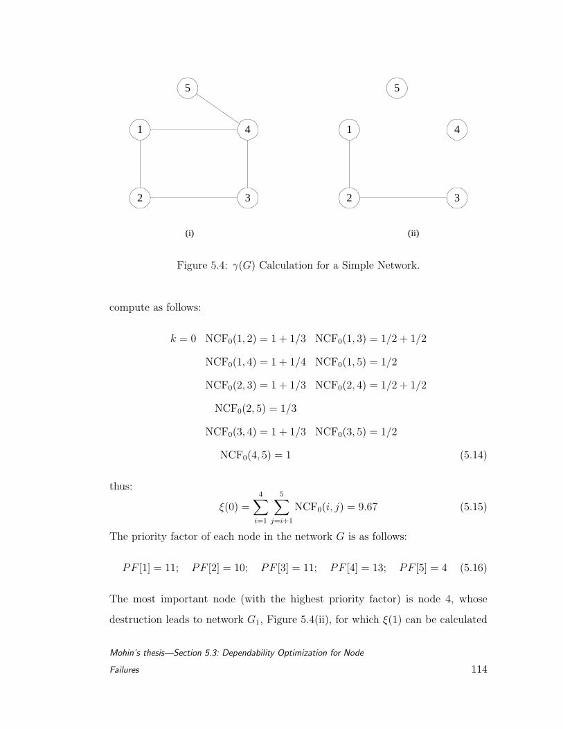
1

2 3

4

5

1

2 3

4

5

(i) (ii)

Figure 5.4: γ(G) Calculation for a Simple Network.

compute as follows:

k = 0 NCF0(1, 2) = 1 + 1/3 NCF0(1, 3) = 1/2 + 1/2

NCF0(1, 4) = 1 + 1/4 NCF0(1, 5) = 1/2

NCF0(2, 3) = 1 + 1/3 NCF0(2, 4) = 1/2 + 1/2

NCF0(2, 5) = 1/3

NCF0(3, 4) = 1 + 1/3 NCF0(3, 5) = 1/2

NCF0(4, 5) = 1 (5.14)

thus:

ξ(0) =4∑

i=1

5∑j=i+1

NCF0(i, j) = 9.67 (5.15)

The priority factor of each node in the network G is as follows:

PF [1] = 11; PF [2] = 10; PF [3] = 11; PF [4] = 13; PF [5] = 4 (5.16)

The most important node (with the highest priority factor) is node 4, whose

destruction leads to network G1, Figure 5.4(ii), for which ξ(1) can be calculated


Failures 114

in a similar manner:

ξ(1) = 1 + 1/2 + 1 = 2.5 (5.17)

In this case, the important node is node 2, with PF[2]=3, and its removal leaves

the network completely isolated. Therefore m=2 and thus:

γ(G) = ξ(0) + ξ(1) = 9.67 + 2.5 = 12.17 (5.18)

For the defined DNRC metric, the key idea in the calculations is to remove

the most important node first (the node with the highest priority factor), which

results in a substantial savings in computation time. This implies that the metric

captures the worst case situation of the most important node being destroyed first,

and is therefore a lower bound on the dependability of the network as a whole.

Furthermore, the metric has also combined the effects of link failures associated

with a node failure. It is thus a combined dependability metric that is directly

applicable to the NGI network, as discussed in Chapter 4. It is also applicable

to other types of data fusing sensor network architectures such as those that are

charaterized by having a small number of processing nodes supported by a dense

sensor mesh (Chapter 2).

5.3.2 Simulation Study of the DNRC Metric

To verify the proposed dependability metric, we have automated the computa-

tions discussed in Section 5.3.1 on the MATLAB simulation environment, with

C/C++ customizations. Standard data structures for graph representations, via

adjacency and incidency matrices, were programmed for medium scale networks

of up to 50 nodes. The scenario consisted of n static nodes representing, for ex-

ample, sensor nodes in a data fusion architecture, with n ≤ 50. The subsequent

steps in the simulation are summarized below:


Failures 115

Algorithm 5.1 (DNRC Simulation).

• Input constants (set ‘a priori’): Randomly generated graph G adjacency

and incidency matrices.

• Output : calculated DNRC and P values (probability that remaining net-

work is still connected).

• Initialization Step: Arbitrarily chose e À n links among the pairs of the

nodes in the network, to simulate a randomly designed, connected, network

architecture G, with a small diameter, typically Diam(G) ≤ 2 or 3.

• Calculate D0, the baseline DNRC measure for the random graph.

• While iteration count ≤ 1000, DO:

1. Randomly disable 50% of the nodes in the graph, along with the ad-

jacent edges.

2. Determine if the resulting graph is still connected. Update count.

3. Reset to original graph G and repeat.

• Estimate P, the fraction of the instances when the network was still con-

nected.

The probability value, P, is the Monte Carlo simulated quantification of the

likelihood of the network remaining connected despite suffering upto a 50% de-

struction of its nodes. Higher P values for a particular architecture imply that

network is more dependable and fault tolerant of node failures. On the other

hand, the DNRC values are computed for the same network as prescribed by

Equation (5.11).


Failures 116

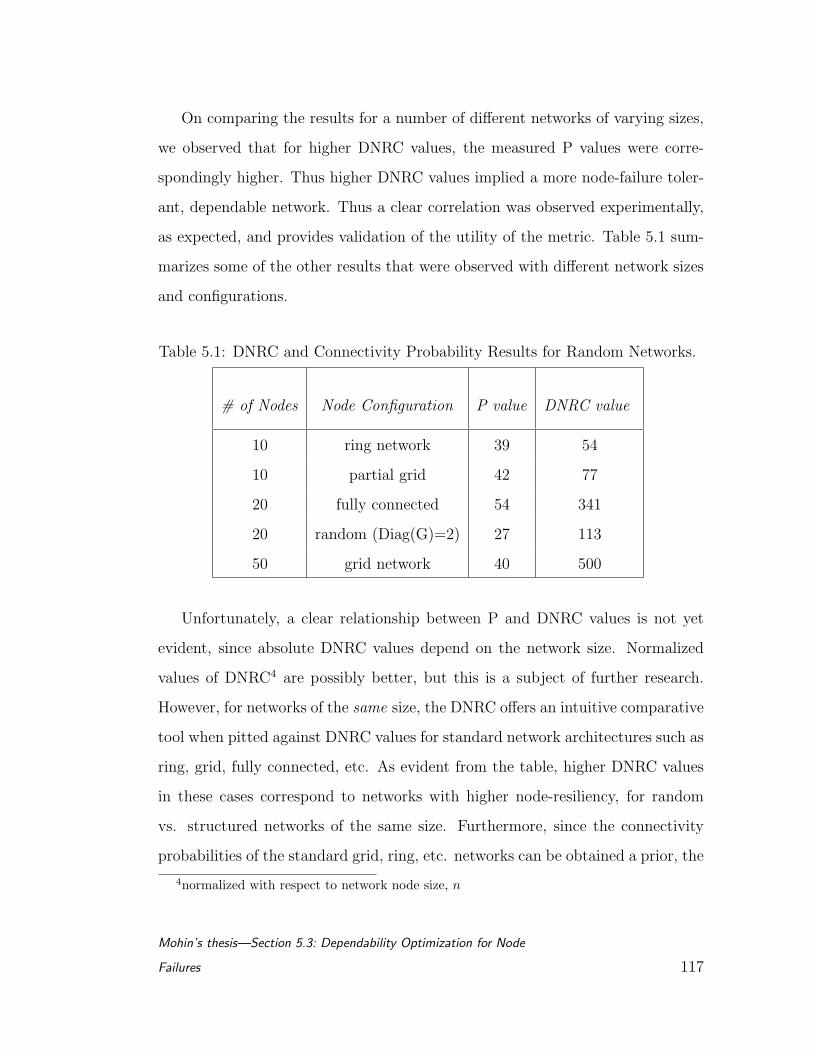
On comparing the results for a number of different networks of varying sizes,

we observed that for higher DNRC values, the measured P values were corre-

spondingly higher. Thus higher DNRC values implied a more node-failure toler-

ant, dependable network. Thus a clear correlation was observed experimentally,

as expected, and provides validation of the utility of the metric. Table 5.1 sum-

marizes some of the other results that were observed with different network sizes

and configurations.

Table 5.1: DNRC and Connectivity Probability Results for Random Networks.

# of Nodes Node Configuration P value DNRC value

10 ring network 39 54

10 partial grid 42 77

20 fully connected 54 341

20 random (Diag(G)=2) 27 113

50 grid network 40 500

Unfortunately, a clear relationship between P and DNRC values is not yet

evident, since absolute DNRC values depend on the network size. Normalized

values of DNRC4 are possibly better, but this is a subject of further research.

However, for networks of the same size, the DNRC offers an intuitive comparative

tool when pitted against DNRC values for standard network architectures such as

ring, grid, fully connected, etc. As evident from the table, higher DNRC values

in these cases correspond to networks with higher node-resiliency, for random

vs. structured networks of the same size. Furthermore, since the connectivity

probabilities of the standard grid, ring, etc. networks can be obtained a prior, the

4normalized with respect to network node size, n


Failures 117

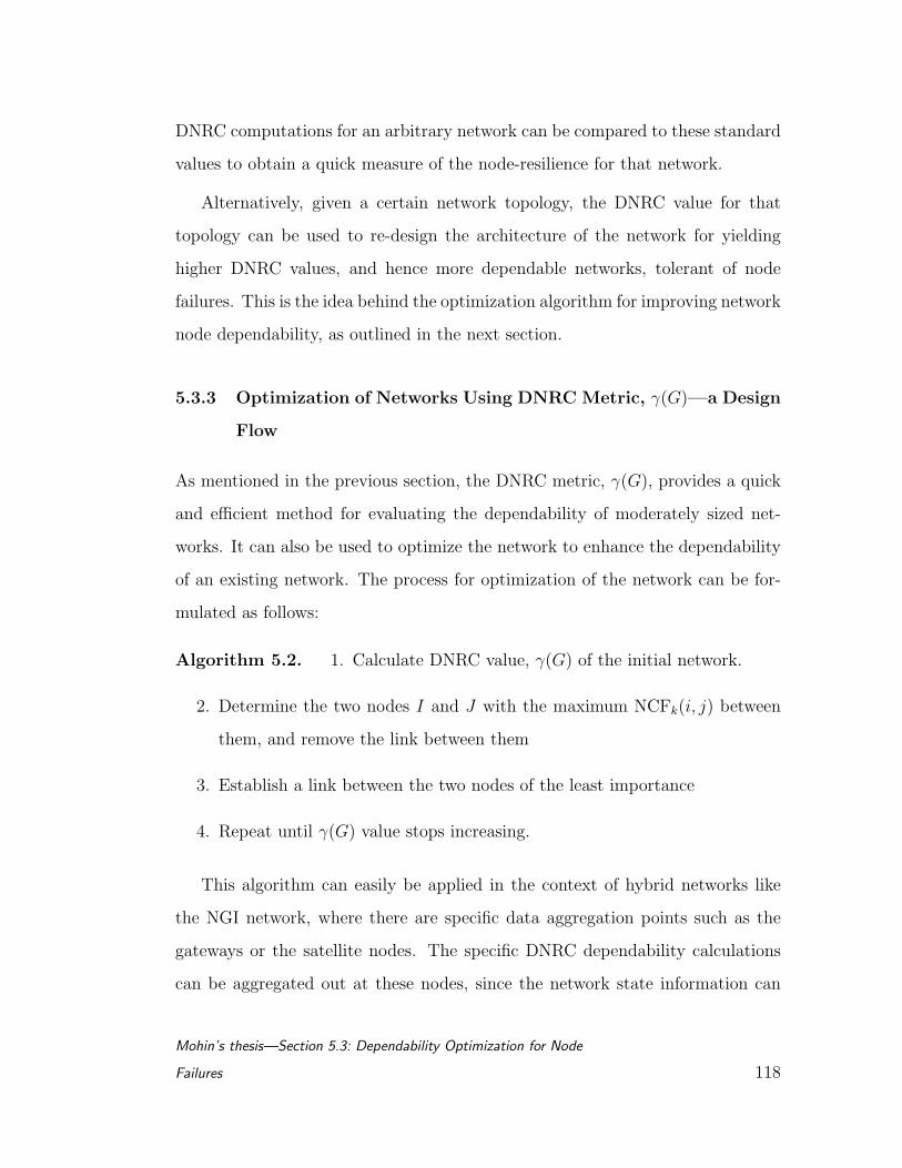
DNRC computations for an arbitrary network can be compared to these standard

values to obtain a quick measure of the node-resilience for that network.

Alternatively, given a certain network topology, the DNRC value for that

topology can be used to re-design the architecture of the network for yielding

higher DNRC values, and hence more dependable networks, tolerant of node

failures. This is the idea behind the optimization algorithm for improving network

node dependability, as outlined in the next section.

5.3.3 Optimization of Networks Using DNRC Metric, γ(G)—a Design

Flow

As mentioned in the previous section, the DNRC metric, γ(G), provides a quick

and efficient method for evaluating the dependability of moderately sized net-

works. It can also be used to optimize the network to enhance the dependability

of an existing network. The process for optimization of the network can be for-

mulated as follows:

Algorithm 5.2. 1. Calculate DNRC value, γ(G) of the initial network.

2. Determine the two nodes I and J with the maximum NCFk(i, j) between

them, and remove the link between them

3. Establish a link between the two nodes of the least importance

4. Repeat until γ(G) value stops increasing.

This algorithm can easily be applied in the context of hybrid networks like

the NGI network, where there are specific data aggregation points such as the

gateways or the satellite nodes. The specific DNRC dependability calculations

can be aggregated out at these nodes, since the network state information can


Failures 118

Figure 5.5: Flowchart for CCA or ‘Aggregation’ Node Local Computation for

Optimizing Reliability

be queried most easily from these locations these locations (e.g. position, load-

ing, BER values that are forwarded to the gateway nodes as part of the route

update messages). In this manner, the route themselves can be updated and

links explicitly instructed to be turned on or off according to the results of the


Failures 119

γ(G) calculations. The flowchart of the algorithm can be summarized as given

in Figure 5.5.


The technique presented in the previous sections provides a form of Reliability

Based Node/Route Selection Process for enhancing the dependability of a peer-

to-peer wireless network. We have provided a platform model on which to ana-

lyze hybrid networks, and defined a novel measure for the dependability of such

networks. The computational process involved in calculating the dependability

measure for an arbitrary network was seen to be a tractable iterative algorithm

which enabled us to create a network design flow (for moderate sized networks)

for improving the reliability of the network.

5.4 Case Study: Dependability Protocols for the NGI

Network

Thus far, we have discussed techniques for the dependability analysis and design

of general peer-to-peer networks, and Section 5.3 in particular introduced tech-

niques for node failures in moderately sized (primarily static) networks. In this

section, we apply and extend these ideas to the canonical example of the DARPA

proposed Next Generation Internet network, which is a hybrid, multi-tiered, het-

erogeneous “network of wireless networks”, as discussed in detail in Chapter 4.

We will consider this as a case study for devising fault tolerance techniques that

will improve dependability of this hybrid network at the points of its maximum

vulnerability—the gateway nodes.

Mohin’s thesis—Section 5.4: Case Study: Dependability Protocols

for the NGI Network 120

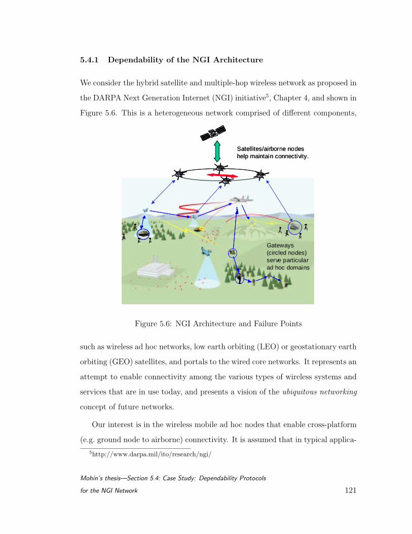
5.4.1 Dependability of the NGI Architecture

We consider the hybrid satellite and multiple-hop wireless network as proposed in

the DARPA Next Generation Internet (NGI) initiative5, Chapter 4, and shown in

Figure 5.6. This is a heterogeneous network comprised of different components,

Satellites/airborne nodeshelp maintain connectivity.

Gateways (circled nodes) serve particular ad hoc domains

Satellites/airborne nodeshelp maintain connectivity.

Gateways (circled nodes) serve particular ad hoc domains

Figure 5.6: NGI Architecture and Failure Points

such as wireless ad hoc networks, low earth orbiting (LEO) or geostationary earth

orbiting (GEO) satellites, and portals to the wired core networks. It represents an

attempt to enable connectivity among the various types of wireless systems and

services that are in use today, and presents a vision of the ubiquitous networking

concept of future networks.

Our interest is in the wireless mobile ad hoc nodes that enable cross-platform

(e.g. ground node to airborne) connectivity. It is assumed that in typical applica-

5http://www.darpa.mil/ito/research/ngi/



tions of the NGI network concept, users forming ad hoc networks will be clustered

into separate mobile groups or domains, e.g. in troop deployments involving mul-

tiple independent platoon units. The objective, then, is to enable reliable, secure

communications among the various node elements across different, geographically

disparate domains. Relatively powerful mobile gateway nodes, which are nodes

that are capable of interfacing between the various hybrid components of the

network are also deployed in the domain of each cluster of nodes, to facilitate

communication with a LEO or GEO satellite, or with each other. Hence, these

gateway nodes serve to extend the range and connectivity of the clusters of mo-

bile nodes. The environment is characterized by the presence of terrain blockages

or other severe channel impairments.

Since the gateways are expected to be the only nodes among the (ground-

based) nodes to be equipped with multi-protocol capable radios, consequently,

all the communication from the ad hoc network to other components of the NGI

extended network have to be routed through these gateway nodes. Any node in

an ad hoc network that wishes to send data to a node in another ad hoc network

that is part of the NGI infrastructure has to first route the data packets to

the gateway. The gateway then forwards them to the appropriate gateway in the

destination ad hoc network, which in turn forwards the packets to the destination

node. However, for this chain of events to execute successfully, each node in the

extended network needs to be configured with the information for identifying the

gateway that it is affiliated with. If only a single gateway is present in each ad

hoc network, then the job of configuring each node with gateway information

is not difficult. As in wired LANs, the mobile nodes can be configured either

manually or during IP address assignment using DHCP.

However, from a fault tolerance point of view, a gateway based architecture



is undesirable because it has catastrophic single points of failure. If each network

domain has just one gateway, then the failure of that gateway will disconnect

that ad hoc network from the NGI infrastructure. The disadvantages of using a

hierarchical network, such as NGI, are well known for distributed systems in gen-

eral, and was discussed in Section 2.4.1. However, for the NGI architecture, there

are no other viable alternatives, since the communication systems involved rely

on different physical and network layer protocols, so gateway or bridge nodes

are the only portal through which common data can be exchanged. This in-

troduces a serious bottleneck at the gateway node, both from a network load

performance and from a dependability perspective. As discussed in Section 4.3.2,

a viable, simple solution to this dilemma is to introduce redundant gateways in

each sub-domain of the network. The redundancy provides a measure of fault

tolerance, and eases the load on any one gateway node—provided that the net-

work signalling and management operations for coordinating multiple gateways

are handled efficiently. Furthermore, all gateways may not be able to communi-

cate with LEO satellites at all times for various reasons (e.g. terrain blockages,

buffer overflows, etc.). In such cases, at least one other gateway-capable node

needs to take over the responsibility of being the gateway for the group, and the

mobile nodes within its purview need to be informed to route their inter -domain

packets to the new gateway. Unfortunately, standard Internet inter-domain rout-

ing protocols like BGP do not apply in these cases because of the high frequency

of changes that is likely in an ad hoc network.

Thus, one of the end objectives of this section is to determine a group of

protocols that enable gateways to efficiently incorporate security and a measure

of dependability and distributed fault tolerance during their normal operations.

In the following sections, we demonstrate mechanisms by which the mobile gate-

ways can alternate amongst themselves the task of being the primary gateway



providing cross layer connectivity, and thus ensure fault tolerance in case of gate-

way failures. These techniques also address the security problem associated with

gateway-centric operations in tactical applications, when critical gateways may

be commandeered or maliciously controlled to disrupt the network. To avoid this

situation, the responsibility of being the gateway should be rotated among the

gateway-capable nodes at pseudo-random times, in an authenticated, distributed

manner. This serves to protect the gateway resource from hostile attacks on the

system that may compromise the connectivity or data integrity of the network.

Time-out conditions can also be set so that if a gateway fails and thus cannot

communicate its status, then the other gateway-enabled nodes would take over

the responsibility autonomously.

In the following sections, these issues are addressed systematically for de-

pendability optimization of gateway-centric, hybrid, multi-tiered networks. In

particular, the following are novel applications of the dependability concepts, as

discussed in this chapter:

• Fault tolerance algorithms by which the network can detect failures among

gateways, and can coordinate the selection and initiation of backup gate-

ways.

• A technique for enabling a random and secure mechanism for rotating the

responsibility of being a gateway among a group of gateway-capable nodes.

This is done by modifying and reducing to practice standard distributed

processing techniques based on generalized Byzantine fault-tolerance algo-

rithms. The algorithms have been specialized to apply to the case of mobile,

wireless gateways.

• The design of the relevant network control features such as routing and



medium access control messaging, to implement the secure and distributed

fault tolerance.

• An implementation and simulations study of the proposed algorithms, uti-

lizing standard DSDV and DSR routing algorithms [79] to estimate over-

head and throughput performance.

5.4.2 Prior Research

It is somewhat surprising that scant literature exists that addresses distributed

fault tolerance and reliability design for ad hoc networks explicitly. A wealth of

literature exists regarding centralized wireless schemes, such as cellular telephony,

but peer-to-peer network reliability has been relegated to the best efforts of the

routing and MAC layer protocols, with no particular system design approach for

hybrid networks.

Several routing protocols, for e.g., DSR [41], DSDV [68], and TORA [66] have

been proposed for ad hoc networks. Almost all of these algorithms are targeted

for routing within the ad hoc network only. They do not extend to heterogeneous

networks containing a mix of both ad hoc components and infrastructure-based

networks. As discussed earlier, such a setup has multiple gateways present within

network that are capable of routing packets between the ad hoc network and the

other types of fixed or airborne networks. Anycasting is a possible solution where

all the gateways can be grouped into a single anycast address and mobile nodes

can use this address as the router for communicating with hosts not in their ad

hoc network. But not all routing protocols support such anycast mechanisms.

Vaidya et al. [45] propose extensions to TORA to support anycasting and Dante,

et al. [38] propose a sink based anycast routing protocol.



Haas, et al. [104] discuss the security related issues related to routing in

ad hoc networks and propose that ad hoc networks should have a distributed

architecture with no central entities to achieve high survivability. They propose

to use (n, t+1) threshold cryptographic methods to decentralize any cryptographic

operation (e.g., signing a key), where at least t + 1 nodes have to collaborate to

perform the operation and no t nodes can achieve the same result, even operating

in collusion.

Any fault tolerant algorithm has to be inherently distributed. The complexity

of such algorithms in ad hoc networks is elevated due to the highly dynamic nature

of such networks and the unreliability of the communication medium. Hatzis, et

al. [35] propose two distributed leader election algorithms for ad hoc networks.

Their algorithms require that all nodes know the coordinates of the space in

advance. In contrast, Malpani, et al. [57] propose distributed leader election

algorithms that are based on TORA. However, both these works consider only the

dynamic and multi-hop nature of the mobile ad hoc network and assume that the

communication medium is reliable and that the nodes are ‘well-behaved’. Other

distributed problems solved for the mobile ad hoc networks are mutual exclusion

[98], and reliable broadcast [65]; however, none of these deals with the case of

misbehaving or malicious nodes.

In contrast to these efforts, we propose distinct algorithms for handling dis-

tributed gateway failures in a hierarchical setting, and study the overhead and

throughput performance in a detailed simulation environment (Section 5.4.5.

5.4.3 Failure Recovery Modes for Gateways in Hybrid Network

We now discuss the general techniques for recovering from gateway failures in

a multi-tiered wireless ad hoc network. In general, hierarchical or centralized



controllers for distributed processing can face a variety of failure conditions during

their normal operations. In the context of wireless gateways in a mobile ad hoc

network setting, these failures can be classified into the following three broad

groups:

(i) Fail-stop: This happens when a gateway is destroyed or otherwise incapac-

itated.

(ii) Intermittent: This can occur when gateways are disabled temporarily be-

cause of terrain blockages, etc.

(iii) Byzantine: This happens when a gateway is confiscated and is being ma-

nipulated by the enemy.

In the following subsections, we propose combined algorithms that can handle

the first two types of failures mentioned above, and also formulate a distributed

algorithm for the third type of failure, based on the standard Byzantine Generals

algorithm, for gateway selection.

5.4.3.1 Fail-stop Behavior and Intermittent failures

We consider both case (i): fail-stop failures, and case (ii): intermittent failures

together, since they can be handled by similar techniques. In fail-stop failures,

the number of gateway-enabled nodes that are available in an ad hoc group

is permanently reduced (through destruction or power/operational outage). In

contrast, for intermittent type failures, gateway nodes are temporarily disabled as

these nodes experience intermittent satellite connectivity (or terrain blockages).

But in this case, the total number of simple nodes (non-satellite connected nodes)

increase since the gateways then become simple nodes.



There are several solutions by which these failures can be handled. These

solutions can be broadly divided into two categories:

(i) Mobile node initiated.

(ii) Gateway initiated.

The solutions for each category can also be sub-divided into two types:

1. Reactive

2. Proactive

Thus there are four possible combinations of solutions, and the algorithms

corresponding to these solutions are outlined in Section 5.4.4.1, and presented

in flowchart and algorithmic form in Section 5.4.7. For estimating the numerical

order for the control messages generated for each strategy, we assume a network

consisting of m mobile nodes and n gateway nodes, per ad hoc network domain.

5.4.3.2 Gateway Byzantine Faults

The more difficult fault arises when a gateway is confiscated and is being manip-

ulated by enemy. The confiscated/manipulated node is henceforth referred to as

the malicious gateway. The fundamental problem that arises as a result is that if

this node manages to assume the role of the gateway for the network, either du-

ring the regular gateway rotation step or by subterfuge, then all communication

in the system is rendered insecure, or worse. The ideal fault tolerance goal for

this scenario will be to prevent the malicious node from becoming the gateway,

or interfering in the gateway selection or data routing tasks.



A gateway, when active, attracts a lot of communication from nearby mobile

nodes, as part of it regular function of routing inter-domain packets. However,

an analysis of the traffic pattern might reveal the position information of the

active gateway, and thus making it susceptible to attacks or confiscation. To

avoid these problems (as well as for power conservation reasons), it is clear that

no gateway should be active for long periods. Instead, the task of being the

gateway in a domain should be rotated among the gateway-capable nodes in

that local network. In addition, no mobile node should use same gateway for

communication for long periods. This is to avoid a malicious node claiming to

be active and manipulating the packets from that mobile node. This also avoids

the collection of contiguous encrypted packets of data by the malicious gateway,

where the contiguity may become helpful in decrypting the data or revealing of

the key used to encrypt the data.

Thus, an algorithm is required that assigns the role of the gateway among

the gateway-enabled nodes in a pseudo-random fashion. Any such algorithm

that selects active gateways and configures the nodes with at least one gateway

should follow three criteria:

(i) No gateway should be allowed to be active for long period of time.

(ii) No mobile node should use a single gateway for long period of time.

(iii) The order in which gateways become active should not be pre-decided or

predictable.

If the selection sequence is pre-decided, then a confiscation of a gateway will

allow the malicious node to know in advance exactly the times when each gateway

becomes active. It will also know which gateway is being used by each mobile

node. To avoid this vulnerability, any gateway selection algorithm should follow



the following third criterion: i.e., gateways that will become active for a time

period should be selected just prior to that time period, by at least a majority of

gateways participating in the selection procedure. This is a distributed majority

selection problem, which is a modified form of the ‘Byzantine Generals Problem’

that has been extensively studied [49]. For the case of gateways in mobile ad hoc

networks, we have modified the general algorithm and reduced to practice the

essential algorithm that satisfies all the three criteria mentioned above. This is

discussed in Section 5.4.4.2, and flowcharts and pseudo-code are also included in

Section 5.4.7.

5.4.4 Algorithms for NGI Gateway Fault Tolerance and Security

We now discuss the algorithms for the four possible combinations of solutions for

recovering from gateway failures, as mentioned earlier, as well as from Byzantine-

type faults for a multi-tiered wireless ad hoc network. The fault tolerance algo-

rithms that we propose are designed to be implemented as hardware or software

protocols on computing devices operating as part of a wireless network. They rely

on underlying and overlying systems and software modules for complete system

operation. As such, our assumptions regarding the NGI system architecture are

as follows:

Assumptions Regarding NGI Architecture for Fault Tolerant System Design

• The fault tolerance algorithms are network programs residing at the network

layer and/or transport layer of the 7 layer OSI stack. They will interact with

the routing protocol to direct the formation/destruction of routes within

the ad hoc network.

• The network employs standard MAC, Routing or Physical Layer protocols.



• The network may have application level or packet level encryption/data

authentication, but strong encryption and mutual authentication is an ab-

solute necessity for passing the control messages among the gateways exe-

cuting the fault tolerance algorithms. This is to ensure against Byzantine

attacks from unauthorized nodes.

• During initial deployment, all the gateway-capable nodes in an ad hoc net-

work are aware of each other’s identity (e.g. authentication public key,

network address etc.).

• During normal operations, only one gateway per ad hoc group is active as

the primary gateway for that domain. Backup gateways are activated (one

at any given time) in response to failures or for security/alteration reasons.

There is no system architectural reason that prevents multiple gateways

from operating simultaneously. However, simulation studies have suggested

that the overhead necessary (in handoff, tracking, power conservation etc.

for the mobile nodes in the group) for multiple operational gateways per

group outweighs the benefits.

• During initialization and boot-up, the gateway node with the lowest net-

work ID assumes the task of being the gateway and floods the network with

this identification information. Standard underlying protocols are assumed

to ensure authentication (e.g. by digital signatures, etc.) for the other

nodes in the network.

• Since gateway nodes are expected to be GPS enabled, a common synchro-

nization clock is assumed to be available to all the gateway nodes for rec-

onciling time-out clocks and timers for the distributed algorithms.



5.4.4.1 Fail-stop or Intermittent Failure Recovery Algorithms

Mobile initiated and Reactive

In this case, each mobile node starts a search for a gateway only if it finds its

current gateway to be inactive. The detailed algorithm is shown in flowchart form

as Figure 5.7 with the accompanying pseudo-code, in Section 5.4.76. To check the

‘liveness’ status of its current gateway (which indicates whether it is operating

or dead), the mobile node pings the gateway periodically. Each mobile node

periodically sends gateway STATUS query message to its current gateway and

expects a KEEP ALIVE message as the reply within an RTT amount of time.

If no such reply is received, the mobile node broadcasts a gateway SOLICIT

message and waits for a reply from any active gateway for T2 time. The mobile

node keeps retrying for every T2 time until an active gateway sends a gateway AD

message. This whole procedure is repeated every T1 units of time. The broadcast

messages need to reach beyond a single hop in the ad hoc network; consequently

all nodes rebroadcast a broadcast message upon receiving one for the first time.

The number of messages that flow in the network as a result is n ·1/T1 unicast

messages per unit time. However, when a gateway is determined to be dead, there

will be a flood of n gateway SOLICIT broadcast messages in the worst case, and

n/m broadcast messages for the average case. The replies to gateway SOLICIT

messages are unicast messages and can be up to (m−1) ·n messages in the worst

case and (m− 1) · n/m for the average case.

Mobile initiated and Proactive:

In this case, each mobile node keeps track of all active gateways by periodically

pinging all the gateways. When the current gateway that the node is affiliated

6All the figures and algorithm pseudo-codes for this section are listed together in Section5.4.7 towards the end of this chapter.



with does not respond to ping messages, the node switches to one of the gateways

that recently responded to its ping messages. The detailed description of this

approach is Figure 5.8. This algorithm is similar to the reactive case presented

earlier. The main difference lies in the fact that the mobile nodes have to keep

track of all the gateways in the network. This is useful for fast recovery, if the

current gateway becomes inactive, but at the cost of an increase in the overhead.

The number of messages in the normal case is m · n · 1/T1 unicast messages

per unit time. When a failure is detected, the switch-over time to a new gateway

is close to zero in most cases, and is the same as for the reactive case when no

other gateway responds to gateway STATUS query message.

Gateway initiated and Reactive:

For the gateway initiated reactive case, each gateway keeps track of the active

gateways through a periodic KEEP ALIVE message exchange between them-

selves. Each gateway responds to another gateway’s KEEP ALIVE message

with a KEEP ALIVE ACK message. A particular gateway is labeled as dead

only if this gateway does not respond to fixed number of multiple retries of the

KEEP ALIVE message transmissions. When a gateway is found to be inactive,

all gateways broadcast a gateway AD message that includes information about

all known gateways that are alive. The nodes previously using the dead gateway,

on collecting such messages, can subsequently switch to a new active gateway in

its radio range.

In the reactive case, there is a flow of m · (m− 1) · 1/T1 unicast messages per

unit time and m broadcast messages upon detection of a faulty gateway. The

detection time is T1/2 seconds, on the average.

Gateway initiated and Proactive:

For the gateway initiated proactive case, all gateway enabled nodes period-



ically broadcast a gateway AD message. Each mobile node that receives such

a message from a gateway-enabled node decides whether to switch to this new

gateway based upon on two parameters: (i) hop count, and (ii) last time, Tlast

at which a gateway AD message was received from the current gateway. If the

hop count to the new gateway-enabled node is less than the current gateway’s

hop count to which it is affiliated, or if the condition:

Tlast < 2 · 1

(gateway ad frequency)

is true, then the mobile sets the ‘better’ gateway-enabled node as its new gateway.

Figure 5.10 and the associated pseudo-code explains the actions of the mobile

node and gateways in further detail.

The proactive solution requires m · 1/T1 number of broadcast messages per

unit time, where 1/T1 is the frequency of gateway advertisement broadcasts. The

switchover time upon detection of a faulty gateway is negligible, but the detection

time itself is T1 · (3/2) units, on the average.

The overhead required for the four solutions presented above can be summa-

rized as shown in Table 5.2.

Table 5.2: Overhead Requirements for Gateway Fault Tolerance Algorithms.

Mobile Node Initiated Gateway Initiated

Reactive (m− 1) · nm

unicast, m · (m− 1) · 1T1

unicast,

nm

broadcast m broadcast

Proactive m · n · 1T1

unicast m · 1T1

broadcast

Best Solution:

Based on the number of messages exchanged, detection time and switchover

times, for each of the four algorithms presented above, the gateway initiated



solutions are better since they can make use of the connectivity through the

overhead satellite network, and also present low overhead on the communication

infrastructure in the ground-based ad hoc network. In particular, all other things

being equal, the gateway initiated and reactive solution is best because all the

messaging is only between gateways.

5.4.4.2 Gateway Selection Algorithm

The general flowchart of the gateway selection algorithm is shown as Figure 5.11.

The precondition for this algorithm is that every gateway knows the list of all

other gateways in the ad hoc network. We will use the same KEEP ALIVE based

mechanism as described in previous sections. The properties of the gateways we

assume in this system are: (i) the gateways are synchronized (almost synchronized

because of accessibility to GPS for all gateways), (ii) the messages may be lost,

and (iii) not all gateways are reliable.

The algorithm has two phases. During the initialization phase, each gateway-

enabled node looks up its list of all other known gateway-enabled node in its

domain and queries them regarding status (of being dead or alive). Based upon

the status, each gateway-enabled node forms the list of the ‘voting gateways’. In

case there is a malicious gateway among this group of voting nodes, then at least

4 gateway nodes are required to be alive, otherwise the impossibility situation of

the Byzantine Generals Problem occurs [49]. In this case, the default operation

mode would be for each gateway-enabled node to assume the role of being the

gateway to all the nodes within one hop distance of itself (nodes that are within

one hop distance of more than one gateway decides locally which gateway node’s

domain to join). The domain is thus partitioned in this mode (to minimize

the data manipulation activities of the malicious node), and the command and



control center, and all the nodes in the domain are informed of the impossibility

situation. If necessary, then depending upon the application scenario, the nodes

may choose to stop transmitting all sensitive inter-domain data altogether.

If the impossibility situation mentioned above does not occur, and more than

4 gateway nodes are alive, then each gateway-enabled node waits a random time,

T, between 0 to T1max It then generates its vote as to who the next gateway

should be from among the list of the voting gateways, excluding the current

gateway as a possible candidate. This vote is then signed using the underlying

encryption technology that is being used, and transmitted to all the other gate-

ways in the voting list. This is done for all the members of the voting list and

each gateway sends its message and collects the messages sent by other gateways.

Since the communication path between gateways can have intermittent failures,

ACK-based mechanism is used (e.g. IEEE 802.11) to increase the reliability of

message exchange in each round. If more than two-thirds of the votes are re-

ceived by each node before timeout condition T2max, then each gateway performs

a count of the majority vote and if a clear winner emerges, then switches to this

new gateway. All the mobile nodes are then informed of this decision by all the

gateways broadcasting SELECTED gateway messages. If either a timeout occurs

or no majority winner emerges, then the algorithm is repeated (up to a software

settable number of times, depending upon the application requirements). How-

ever, if two-thirds of the votes are not received by the timeout condition, then

once again, the impossibility situation of the Byzantine Generals Problem occurs

and the domain-partitioned default mode of operation is invoked.

The gateway selection algorithm is periodically executed (with large enough

timeout periods T1maxand T2max to prevent too frequent gateway changes). Since

all gateways are almost synchronized, each gateway knows when the selection



algorithm needs to be (re)started. It is interesting to note that this algorithm

may also be used if the currently active gateway is destroyed or its satellite link

is blocked. Thus, it can be used as another variation (albeit inefficient) of the

gateway fault recovery system described earlier.

5.4.5 Implementation of the Gateway Reliability Algorithms

We have simulated the algorithms for gateway fault tolerance, outlined in Section

5.4.3, on the ns-2 network simulation platform, version 2.1b8 [95]. This version

contains modules that implement different wireless network protocols, such as

DSDV, DSR, TORA and AODV. Our simulation setup is similar to that shown

in Figure 5.12, where the ad hoc network component consisted of five mobile

nodes. Some of the mobile nodes are designated as gateways, and are labeled

as BSx in the figure. They serve to connect wireless ad hoc network to the

other components of NGI. The Control Operations Center (COC) is divided into

several components, labeled as COCx. Each normal mobile node, labeled as Nx,

has a TCP connection with corresponding COCx. Depending on the gateway

BSx that a mobile node Nx is using at any time instant, all links from COCx to

all gateways in ad hoc network are disabled, except the link to BSx. This forces

the packets from COCx to Nx to flow through the gateway BSx. A single COC

cannot be used in our ns-2 setup because packets to different mobile nodes need

to be routed through different gateways. In a real-life setup, the COCs would

normally be low earth orbiting satellites, and would have some satellite network

handoff mechanism to decide about which gateway to use.

For preliminary experiments, we performed gateway selection in a round-

robin fashion. In this method, every node in the ad hoc component knows which

gateway will be active at any time instance in advance, according to a fixed time



look-up table. There is no data overhead incurred in gateway selection and no

overhead in the mobile node configuration. The only overhead is due to the

abrupt change in switching from old to new gateway, during which time some

packets may be lost as new routes are established. We compared this case with

best base-station approach. In best base-station approach, each mobile node is

periodically configured to use the nearest gateway (nearest in number of hops).

The experimental setup contained 100 mobile nodes in the ad hoc network,

moving in a rectangular, bounded region of 700mx700m size, at an average speed

of 40 m/s. We generated the movement scenario file using CMU’s setdest tool. We

implemented fault-tolerant agents, referred to as ftagents, which runs on each node

of the ad hoc network. The ftagents on gateways keep track of other gateways,

participate in gateway selection and perform the task of informing all mobile

nodes. The ftagents on nodes receive messages from gateways and configure the

node to use the selected gateway for communicating with the nodes not in same

domain.

The overall throughput for different numbers of gateways, with DSDV as the

underlying routing protocol, is shown in Figures 5.13 and for DSR is shown in

Figure 5.14. In each of the results graphs, we have compared the performance of

the best base-station approach to the round-robin case. The main point to note

from the plots is that the change in the overall throughput is not very significant

for the fault tolerance algorithms, implying that the overhead and computational

load incurred are bearable for the fault tolerance objectives for this system.


Thus far, we have outlined algorithms that provide a measure of fault tolerance

and security in the operation of gateways in a hybrid satellite, mobile multi-hop



network environment. Based on the number of messages exchanged, detection

time and switchover times, for each of the four algorithms presented above, the

gateway initiated solutions are better since they can make use of the connectivity

through the overhead satellite network, and also present low overhead on the

communication infrastructure in the ground-based ad hoc network.

Simulation results obtained by studying some representative cases on the ns-2

simulation platform implied that the algorithms are practical and implement-able,

with only a marginal increase in overhead and complexity.

In summary, we have thus demonstrated that the reliability and dependability

of critical information processing nodes in hierarchical networks such as the NGI

can be enhanced by means of relatively simple fault tolerant, secure protocols.

The techniques employed also enabled the network to be self-recoverable, and to

have a graceful degradation in the network performance in the face of failures—

either unintentional or malicious. These techniques can also be applied to any

hybrid satellite/mobile ad hoc network that is deployed in a terrain with blockages

and communication impairments (e.g. tactical applications involving divisions of

troops communicating with mobile gateways in harsh fading/jammed communi-

cation environments with blockages and high failure hazards). Other applications

can be in distributed robotic platforms, e.g. in terrestrial or extraterrestrial ex-

ploration, where mobile nodes have to operate in possibly inhospitable terrain

(outer space, planetary or earth remote locations) for remote sensing, data col-

lection, control applications, etc. The gateways in such applications can serve as

the central data collection point for various mobile nodes, which are then relayed

to appropriate LEO or GEO points. Thus the gateways in these scenarios have

to be ultra-reliable and secure.

Commercial applications are also possible in industrial settings where mobile



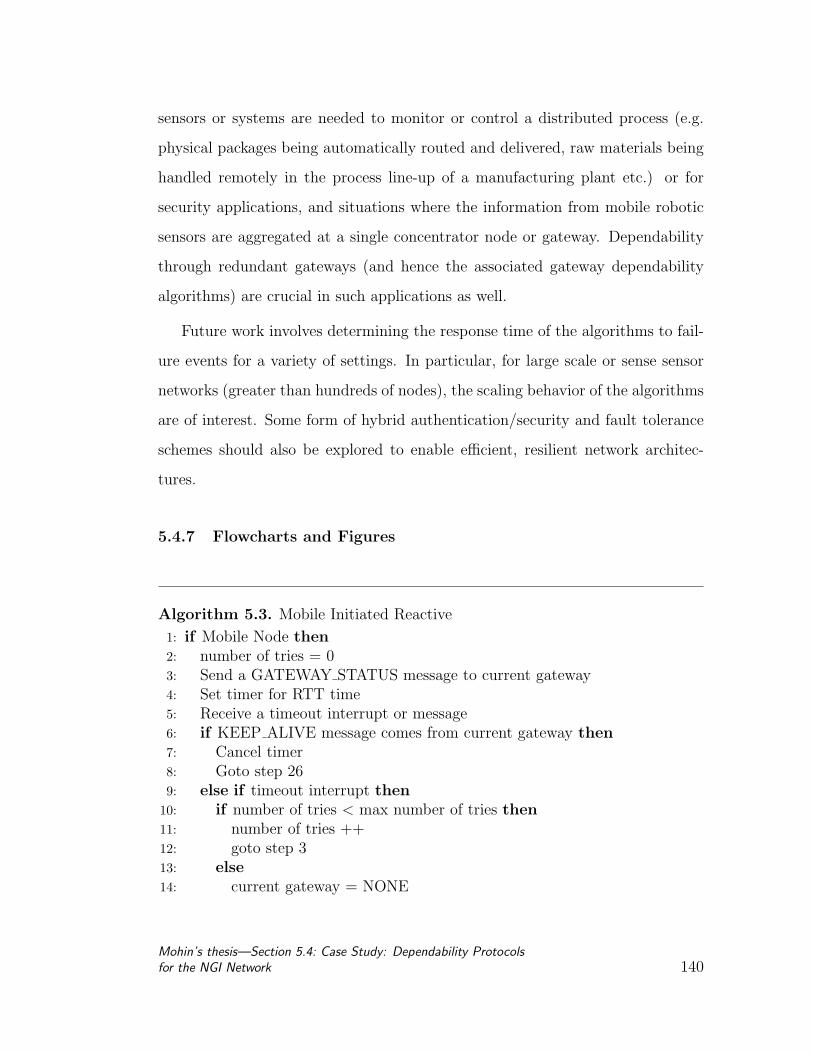
sensors or systems are needed to monitor or control a distributed process (e.g.

physical packages being automatically routed and delivered, raw materials being

handled remotely in the process line-up of a manufacturing plant etc.) or for

security applications, and situations where the information from mobile robotic

sensors are aggregated at a single concentrator node or gateway. Dependability

through redundant gateways (and hence the associated gateway dependability

algorithms) are crucial in such applications as well.

Future work involves determining the response time of the algorithms to fail-

ure events for a variety of settings. In particular, for large scale or sense sensor

networks (greater than hundreds of nodes), the scaling behavior of the algorithms

are of interest. Some form of hybrid authentication/security and fault tolerance

schemes should also be explored to enable efficient, resilient network architec-

tures.

5.4.7 Flowcharts and Figures

Algorithm 5.3. Mobile Initiated Reactive

1: if Mobile Node then2: number of tries = 03: Send a GATEWAY STATUS message to current gateway4: Set timer for RTT time5: Receive a timeout interrupt or message6: if KEEP ALIVE message comes from current gateway then7: Cancel timer8: Goto step 269: else if timeout interrupt then

10: if number of tries < max number of tries then11: number of tries ++12: goto step 313: else14: current gateway = NONE

Mohin’s thesis—Section 5.4: Case Study: Dependability Protocolsfor the NGI Network 140

15: Broadcast a GATEWAY SOLICIT message16: Set timer for T2 time17: Receive a message or timeout interrupt18: if GATEWAY AD received from a gateway G then19: current gateway = G20: Cancel timer21: else if timeout interrupt then22: goto step 1523: end if24: end if25: end if26: Sleep for T1 time27: goto step 228: end if

1: if Gateway then2: Send KEEP ALIVE message to the sender of GATEWAY STATUS mes-

sage3: Send GATEWAY AD message to the sender of GATEWAY SOLICIT mes-

sage4: end if

Algorithm 5.4. Mobile Initiated Proactive

1: if Mobile Node then2: number of tries = 03: Set of responding gateways G = NULL4: Send a GATEWAY STATUS message to all known gateways5: Set timer for RTT time6: Receive a timeout interrupt or message7: if KEEP ALIVE message comes from gateway g then8: if current gateway == g then9: Cancel timer

10: Goto Step 3811: else12: G = G

⋃ g13: Goto Step 614: end if15: else if timeout interrupt then16: if number of tries < max number of tries then


17: number of tries ++18: Send a GATEWAY STATUS message to current gateway19: goto step 420: else21: current gateway = NONE22: if S 6= NULL then23: current gateway = choose one from set S24: Goto step 3825: else26: Broadcast a GATEWAY SOLICIT message27: Set timer for T2 time28: Receive a message or timeout interrupt29: if GATEWAY AD received from a gateway G then30: current gateway = G31: Cancel timer32: else if timeout interrupt then33: goto step 2634: end if35: end if36: end if37: end if38: Sleep for T1 time39: goto step 240: end if

1: if Gateway then2: Send KEEP ALIVE message to the sender of GATEWAY STATUS mes-

sage3: Send GATEWAY AD message to the sender of GATEWAY SOLICIT mes-

sage4: end if

Algorithm 5.5. Gateway Initiated Reactive

1: if Gateway then2: S = set of all gateways3: number of tries = 04: Set of gateways that acknowledge S’ = NULL5: Send a KEEP ALIVE message to all gateways in set S6: Set timer for T2 time


7: Receive a message or timeout interrupt8: if received a KEEP ALIVE ACK message from gateway g then9: S’ = S’

⋃ g10: Goto Step 711: else if timeout interrupt then12: if S == S’ then13: Goto step 2314: else if number of tries < max number of tries then15: number of tries ++16: Send a KEEP ACK message to gateways in set (S-S’)17: goto step 518: else19: S = S’20: Broadcast a GATEWAY AD message including G in the message21: end if22: end if23: Sleep for T1 time24: goto step 325: end if

1: if MobileNode then2: Receive a GATEWAY AD message from gateway G with gateway set S3: if current gateway ∈ S then4: Goto step 25: else6: current gateway = G7: end if8: Goto step 29: end if

Algorithm 5.6. Gateway Initiated Proactive

1: if Gateway then2: Broadcast a GATEWAY AD message3: Sleep for T1 units of time4: Goto step 25: end if

1: if Mobile Node then2: Receive a GATEWAY AD message from gateway G


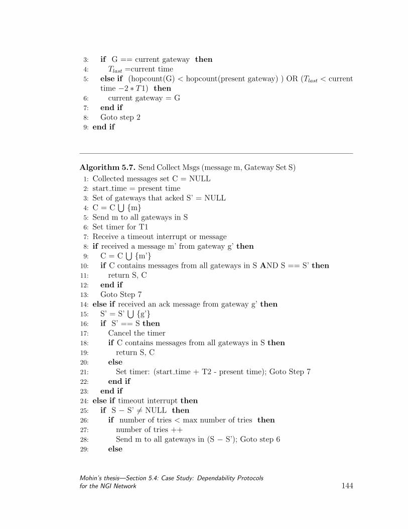
3: if G == current gateway then4: Tlast =current time5: else if (hopcount(G) < hopcount(present gateway) ) OR (Tlast < current

time −2 ∗ T1) then6: current gateway = G7: end if8: Goto step 29: end if

Algorithm 5.7. Send Collect Msgs (message m, Gateway Set S)

1: Collected messages set C = NULL2: start time = present time3: Set of gateways that acked S’ = NULL4: C = C

⋃ m5: Send m to all gateways in S6: Set timer for T17: Receive a timeout interrupt or message8: if received a message m’ from gateway g’ then9: C = C

⋃ m’10: if C contains messages from all gateways in S AND S == S’ then11: return S, C12: end if13: Goto Step 714: else if received an ack message from gateway g’ then15: S’ = S’

⋃ g’16: if S’ == S then17: Cancel the timer18: if C contains messages from all gateways in S then19: return S, C20: else21: Set timer: (start time + T2 - present time); Goto Step 722: end if23: end if24: else if timeout interrupt then25: if S − S’ 6= NULL then26: if number of tries < max number of tries then27: number of tries ++28: Send m to all gateways in (S − S’); Goto step 629: else


30: Label all gateways in set (S − S’) as dead; S = S’31: if C contains messages from all gateways in S then32: return S, C33: end if34: Goto Step 735: end if36: else37: Label all gateways whose messages does not appear in C to be dead38: S = S - dead gateways; return S, C39: end if40: end if

Algorithm 5.8. Check Consistency (message set C)

1: Suppose C = C1, C2, C3, ..., Cm2: G = NULL3: R = NULL4: for all gateway g s.t. g’s message is in at least one c ∈ C do5: if g’s message is in at least f ∗ |C| number of c’s in C then6: G = G

⋃ g7: R = R

⋃ g’s message8: end if9: end for

10: return G, R

Algorithm 5.9. Select Gateway (gateway set G)

1: Choose a random number r2: Calculate MD5 hash(r) = h3: G,c = SendCollectMsgs(h, G) /* Phase 1 Round 1 */4: G,C’ = SendCollectMsgs(c, G) /* Phase 1 Round 2 */5: G, H SET = CheckConsistency(C’)6: G,D = SendCollectMsgs(R, G) /* Phase 2 Round 1 */7: G,D’ = SendCollectMsgd(D, G) /* Phase 2 Round 2 */8: G, R SET = CheckConsistency(D’)9: for all g ∈ G do

10: if MD5Hash(rg) 6= hg then11: G = G - g;12: end if


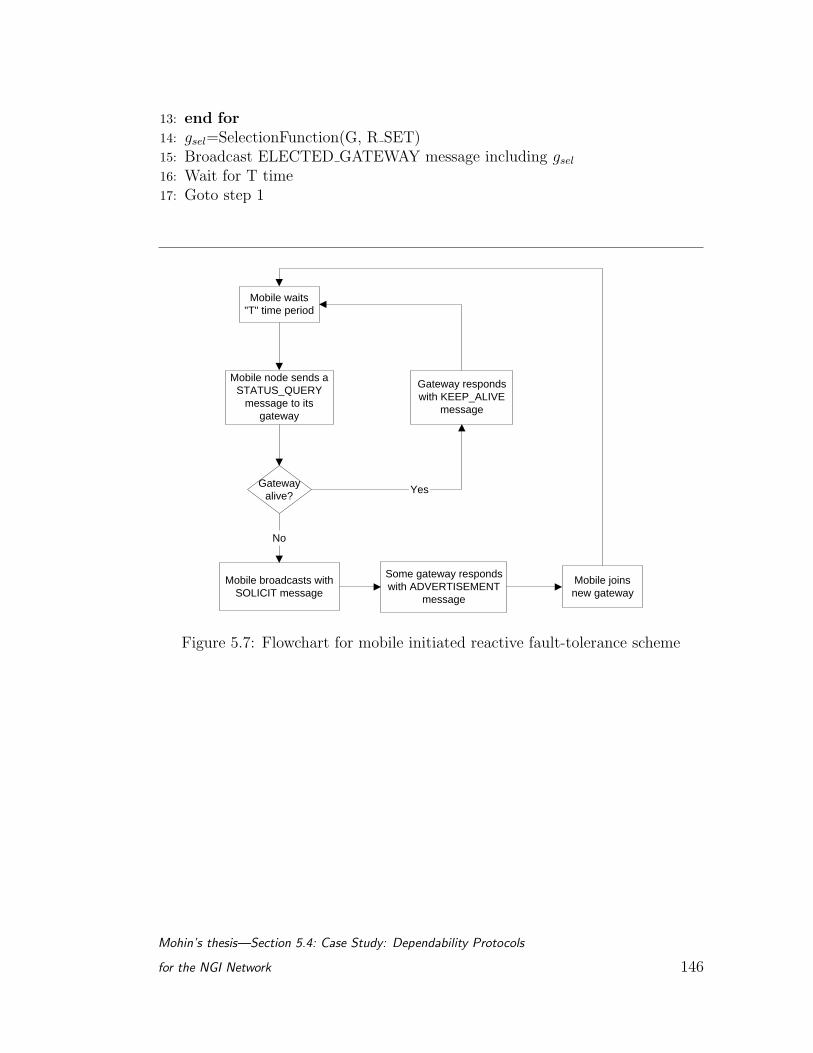
13: end for14: gsel=SelectionFunction(G, R SET)15: Broadcast ELECTED GATEWAY message including gsel

16: Wait for T time17: Goto step 1

Mobile node sends a STATUS_QUERY

message to its gateway

Gateway responds with KEEP_ALIVE

message

Gateway alive?

Mobile broadcasts with SOLICIT message

Mobile waits "T" time period

Yes

No

Some gateway responds with ADVERTISEMENT

message

Mobile joins new gateway

Figure 5.7: Flowchart for mobile initiated reactive fault-tolerance scheme



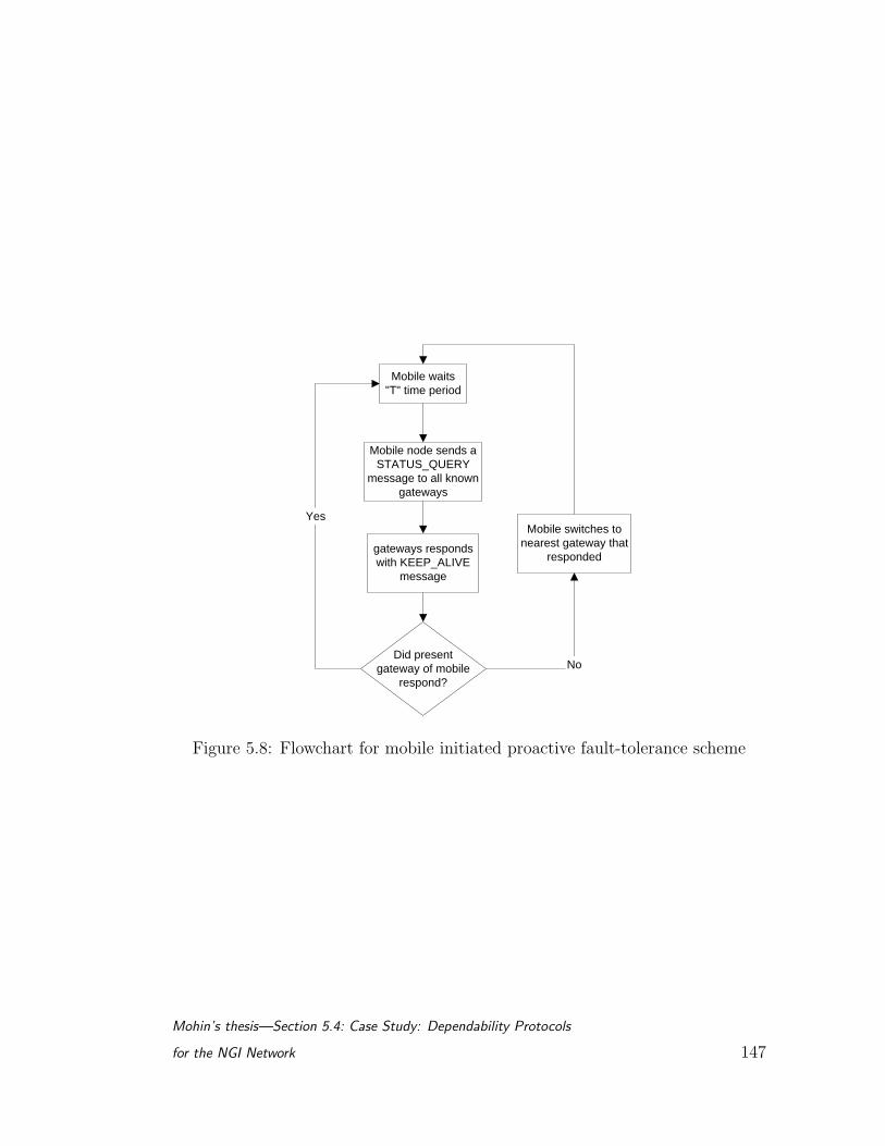
Mobile node sends a STATUS_QUERY

message to all known gateways

gateways responds with KEEP_ALIVE

message

Did present gateway of mobile

respond?

Mobile waits "T" time period

No

Yes Mobile switches to

nearest gateway that responded

Figure 5.8: Flowchart for mobile initiated proactive fault-tolerance scheme



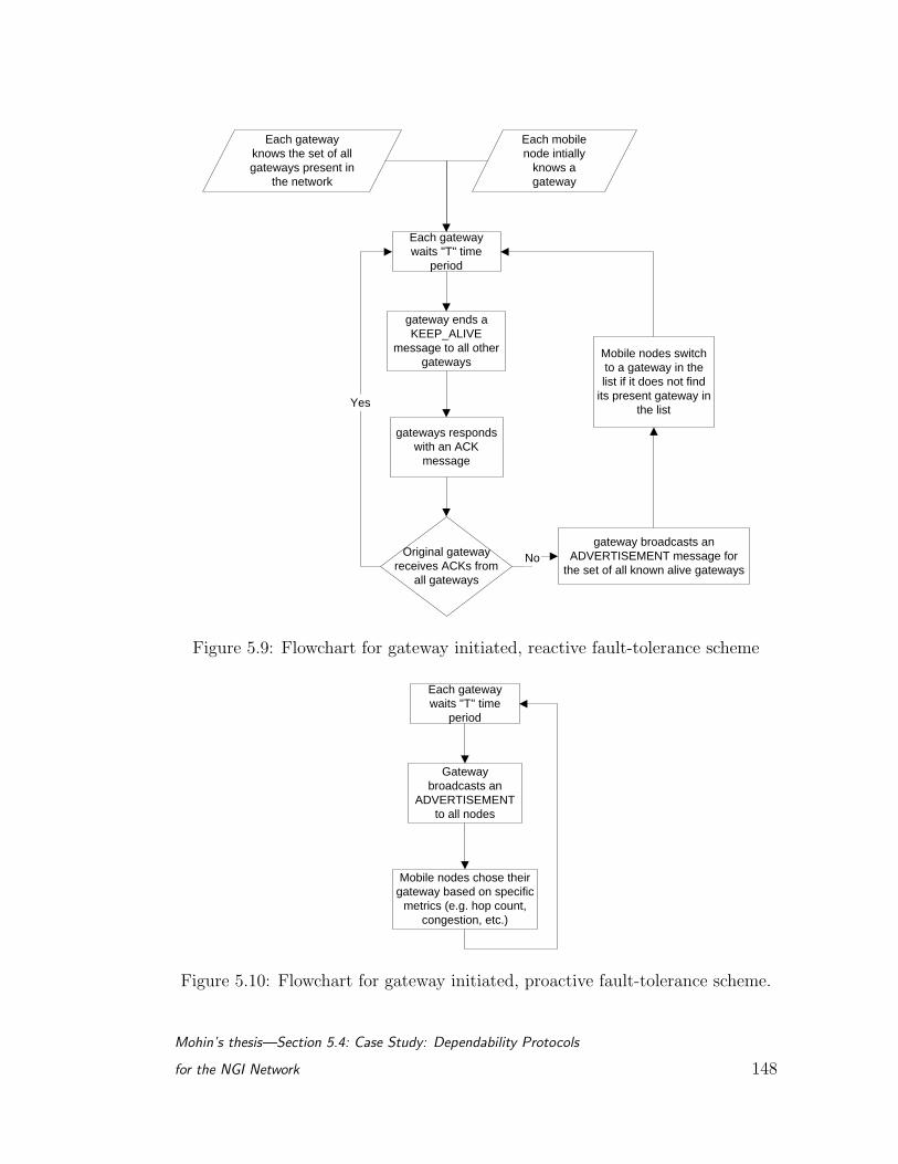
gateway ends a KEEP_ALIVE

message to all other gateways

gateways responds with an ACK

message

Original gateway receives ACKs from

all gateways

Each gateway waits "T" time

period

No

Yes

gateway broadcasts an ADVERTISEMENT message for

the set of all known alive gateways

Each gateway knows the set of all gateways present in

the network

Each mobile node intially

knows a gateway

Mobile nodes switch to a gateway in the list if it does not find

its present gateway in the list

Figure 5.9: Flowchart for gateway initiated, reactive fault-tolerance scheme

Gateway broadcasts an

ADVERTISEMENT to all nodes

Mobile nodes chose their gateway based on specific

metrics (e.g. hop count, congestion, etc.)

Each gateway waits "T" time

period

Figure 5.10: Flowchart for gateway initiated, proactive fault-tolerance scheme.



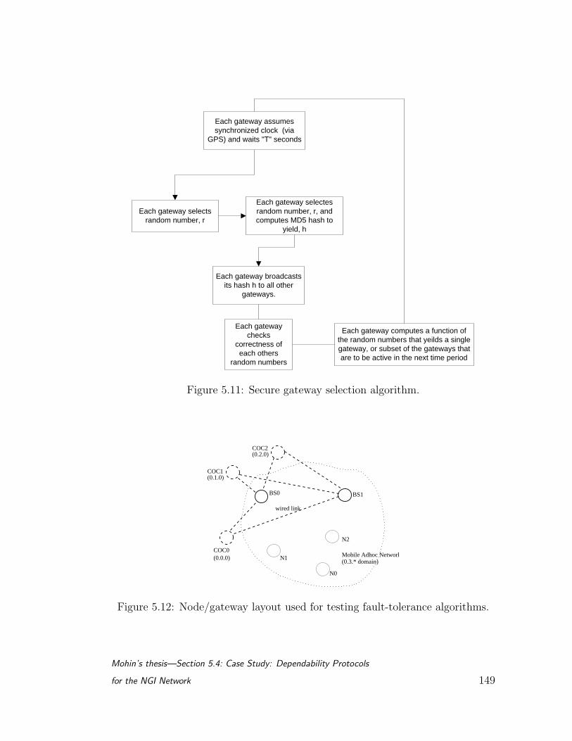
Each gateway selectes random number, r, and computes MD5 hash to

yield, h

Each gateway broadcasts its hash h to all other

gateways.

Each gateway selects random number, r

Each gateway checks

correctness of each others

random numbers

Each gateway computes a function of the random numbers that yeilds a single gateway, or subset of the gateways that are to be active in the next time period

Each gateway assumes synchronized clock (via

GPS) and waits "T" seconds

Figure 5.11: Secure gateway selection algorithm.

BS0 BS1

N1 Mobile Adhoc Network(0.0.0)COC0

wired link

N2

COC1(0.1.0)

(0.2.0)COC2

(0.3.* domain)

N0

Figure 5.12: Node/gateway layout used for testing fault-tolerance algorithms.



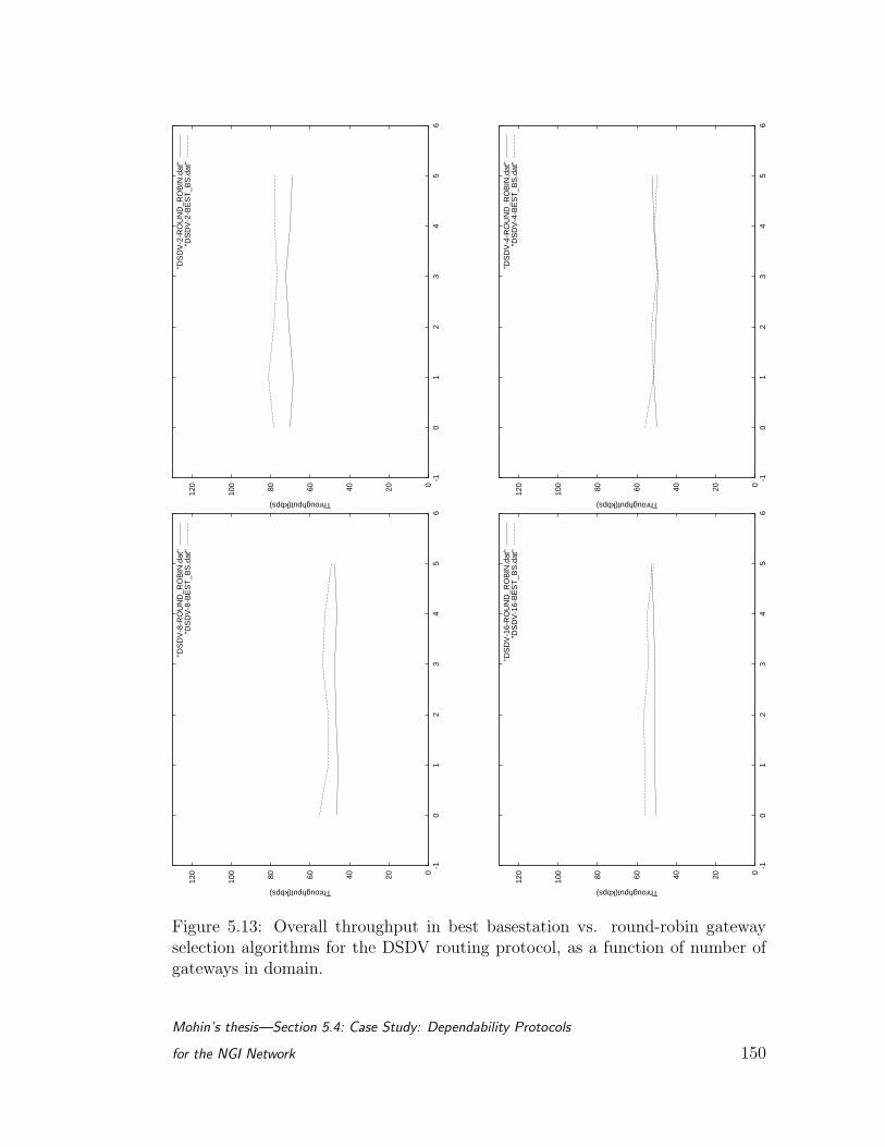
020406080100

120

-10

12

34

56

Throughput(kbps)

"DS

DV

-2-R

OU

ND

_RO

BIN

.dat

""D

SD

V-2

-BE

ST

_BS

.dat

"

020406080100

120

-10

12

34

56

Throughput(kbps)

"DS

DV

-4-R

OU

ND

_RO

BIN

.dat

""D

SD

V-4

-BE

ST

_BS

.dat

"

020406080100

120

-10

12

34

56

Throughput(kbps)

"DS

DV

-8-R

OU

ND

_RO

BIN

.dat

""D

SD

V-8

-BE

ST

_BS

.dat

"

020406080100

120

-10

12

34

56

Throughput(kbps)

"DS

DV

-16-

RO

UN

D_R

OB

IN.d

at"

"DS

DV

-16-

BE

ST

_BS

.dat

"

Figure 5.13: Overall throughput in best basestation vs. round-robin gatewayselection algorithms for the DSDV routing protocol, as a function of number ofgateways in domain.



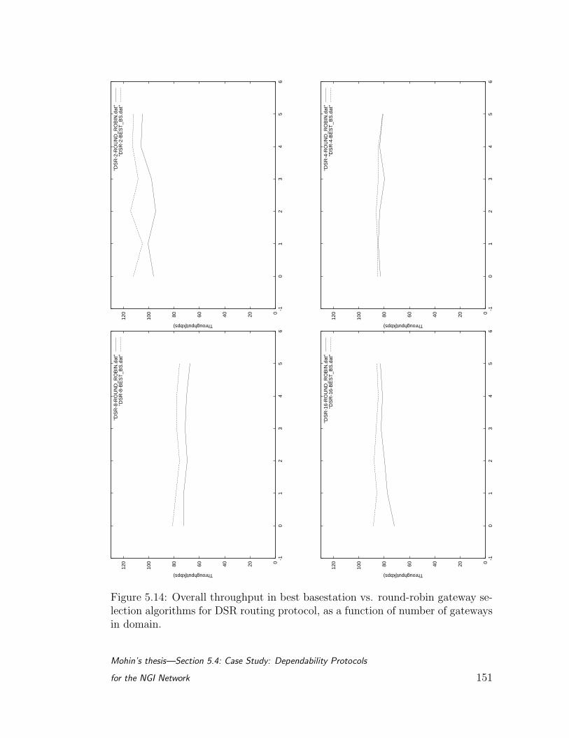
020406080100

120

-10

12

34

56

Throughput(kbps)

"DS

R-2

-RO

UN

D_R

OB

IN.d

at"

"DS

R-2

-BE

ST

_BS

.dat

"

020406080100

120

-10

12

34

56

Throughput(kbps)

"DS

R-4

-RO

UN

D_R

OB

IN.d

at"

"DS

R-4

-BE

ST

_BS

.dat

"

020406080100

120

-10

12

34

56

Throughput(kbps)

"DS

R-8

-RO

UN

D_R

OB

IN.d

at"

"DS

R-8

-BE

ST

_BS

.dat

"

020406080100

120

-10

12

34

56

Throughput(kbps)

"DS

R-1

6-R

OU

ND

_RO

BIN

.dat

""D

SR

-16-

BE

ST

_BS

.dat

"

Figure 5.14: Overall throughput in best basestation vs. round-robin gateway se-lection algorithms for DSR routing protocol, as a function of number of gatewaysin domain.



CHAPTER 6

Rate Adaptive MIMO OFDM LDPC transceiver

The final chapter of this thesis deals with a physical layer issue for wireless

nodes: the design of a rate adaptive transceiver based on multi-input, multi-

output (MIMO) antenna technology, together with some modern modulation and

coding support. The interesting issue about this development is regarding how

information is processed in such a device. It is seen that, in the spirit of Chapter

2 of this thesis, the fundamental techniques that allow signals to be separated

in such devices, and thus allows MIMO to realize its full potential, is a form of

data fusion. The multiple transmit/receive channels can be thought of as inde-

pendent sensor nodes observing independent data, and the challenge is, again,

one of efficient data fusion. Even more interestingly, the techniques that have

been developed over the years in this discipline, and the modified technique that

is proposed, are seen to be case specific implementations of the likelihood fusion

principles discussed in earlier chapters.

The introductory section below outlines the objectives and approaches under-

taken for designing the new radio, and provides a roadway for the subsequent

sections.

152

6.1 Introduction

It was mentioned at the outset that the objective of communication devices can

be generalized to be the acquisition, processing and dissemination of informa-

tion. However, with the exponential rise in the use of wireless devices, the time,

space and frequency dimensions that are necessary to enable all these devices

to operate is becoming crowded. Secondly, as discussed earlier, if the maximum

benefit is to be obtained from these systems, then they need to be networked

in a cooperative communication configuration, and this in turn is placing huge

demands on the available bandwidth. Finally, for most applications involving

wireless devices nowadays, the channel conditions under which these devices are

supposed to operate severely limit the effectiveness of the underlying physical

layer technology. Most wireless channels have very detrimental effects on ra-

dio frequency propagation of communication signals, and essentially constricts

effective bandwidth.

All these constraints have necessitated the development of highly bandwidth

efficient techniques for the physical data transmission/reception functions for

wireless systems of all varieties (sensors, ad hoc node, etc.). In this chapter

of the thesis, an attempt is made to alleviate these problem by presenting a

novel approach that maximizes the raw spectral efficiency of transceivers. This is

accomplished by using a combination of three technologies to form a space-time

coded transceiver that can be adaptively optimized to extract the maximum

diversity from the wireless channel. These technologies are: multi-input, multi-

output antenna technology (MIMO), orthogonal frequency domain multiplexing

(OFDM), and the powerful low density parity check channel codes (LDPC)—

outlined in Sections 6.2.1, 6.2.2, and 6.2.3, respectively.

It has been shown that MIMO technology is the only means by which to


improve upon the Shannon’s hard limit [81] for the capacity of a single antenna

system, also known as single input, single output (SISO) . Over the last few

decades, steady progress has been made in digital communication theory and

practice to the point where the Shannon limit has already been approached using

modern single antenna based coding and modulation techniques [22]. At this

stage, to extract further spectral gains from the wireless channel, MIMO appears

to be the only viable solution. OFDM, on the other hand, is a multi-carrier

modulation technique which has only recently become practically useful with the

advent of powerful FFT and IFFT chipsets [4]. This allows independent data

bits to be sent over smaller individual bins in the frequency spectrum, and thus

counteracts the frequency selective fading effects of the wireless channel, without

the expense and complexity of equalizers. Using OFDM, it then becomes possible

to undo the severe effects of the Rayleigh channel and make the channel appear

more like an AWGN channel. Finally, the newly re-discovered LDPC codes are

powerful channel codes, with performance similar to (or better than) the best

Turbo codes, but having much simpler coding/decoding structures by nature of

being a block code. Over harsh fading channels, it has been shown to achieve

impressive coding gains [56].

Our novel approach has been to combine the best elements of these three

technologies to present a smart, ‘spectrum-aware’, software defined transceiver.

The basic block diagram of the transceiver is shown as Figure 6.1.

In particular, a novel multi-antenna signal separation scheme is proposed,

which uses likelihood decoding of LDPC streams that are transmitted over in-

dependent antennas (Section 6.4.2). Good convergence has been observed in

simulation studies to date. This is coupled with a simplified MIMO channel

estimation scheme that can be incorporated as part of a robust system design


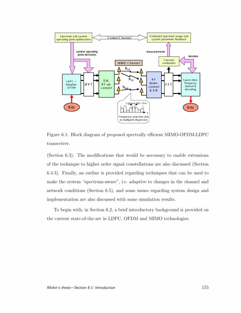
Channelestimation

LDPC + Adaptive

OFDM

Bits

MIMO Channel

Bits

IFFT FFTSpace-time-frequencydemod &decoding

iterative

Spectrum and system operating point optimization Control Channel

measurements

Estimated spectrum usage and system parameter feedback

h11

D/A, RF up-convert

RF down-convert & A/D

h12

Frequency-selective due to multipath dispersion

Coherent BW~1/Tm

f

hmn

system operatingpoint decisions

Channelestimation

LDPC + Adaptive

OFDM

Bits

MIMO Channel

Bits

IFFT FFTSpace-time-frequencydemod &decoding

iterative

Spectrum and system operating point optimization Control Channel

measurements

Estimated spectrum usage and system parameter feedback

h11

D/A, RF up-convert

D/A, RF up-convert



h12

Frequency-selective due to multipath dispersion

Coherent BW~1/Tm

f

hmn

system operatingpoint decisions

Figure 6.1: Block diagram of proposed spectrally efficient MIMO-OFDM-LDPC

transceiver.

(Section 6.3). The modifications that would be necessary to enable extensions

of the technique to higher order signal constellations are also discussed (Section

6.4.3). Finally, an outline is provided regarding techniques that can be used to

make the system “spectrum-aware”, i.e. adaptive to changes in the channel and

network conditions (Section 6.5), and some issues regarding system design and

implementation are also discussed with some simulation results.

To begin with, in Section 6.2, a brief introductory background is provided on

the current state-of-the-art in LDPC, OFDM and MIMO technologies.


6.2 Primer on MIMO, OFDM and LDPC

6.2.1 Multiple Input, Multiple Output (MIMO) Systems

Broadband connectivity has long been considered the future of the telecommu-

nications industry. ‘Broadband’ nowadays typically refers to data services op-

erating at data rates in excess of 1.544 Megabits per second (Mbps), which is

known as the T-1 rate. However, with the explosive growth in the availability

and use of the wireless channel, the available radio frequency spectrum for wire-

less applications has gradually become crowded. Thus, innovative technologies

are now required for optimum spectrum utilization and interference endurance,

while maintaining low-complexity for deployable wireless systems.

This is especially true for mobile ad hoc network (MANET), where low-power,

resource allocation and re-use are of prime concern. In light of these develop-

ments, it has recently been recognized that Multi-input-multi-output (MIMO)

antenna-based radio systems provide marked capacity gain and interference-

combating potential, with manageable system complexity. This is because MIMO

systems with appropriate modulation and coding can better exploit the Space-

Time-Frequency diversity of the wireless channel for maximum spectral efficiency

(measured as the user capacity: bits/sec/Hz/Area, or some physical layer at-

tribute such as bit error rate (BER), outage rate, etc.).

There are also sound system engineering reasons for preferring MIMO systems

as the backbone technology for broadband applications. This is because higher

data rates through single antenna, single carrier systems require expensive equal-

izers/codecs to combat the effects of intersymbol interference (ISI). Multi-carrier

MIMO systems, however, can overcome this constraint, but at the expense of

increased RF processing costs. But historically, the cost of RF processing has

Mohin’s thesis—Section 6.2: Primer on MIMO, OFDM and LDPC 156

grown slower than baseband processing cost as data rates have increased. In ad-

dition, spatio-temporal modems can operate at rates well below their theoretical

limit, while still providing the required throughput, whereas traditional modems

have already been forced to operate in close-to-theoretical operation regions (Fig-

ure 6.3). Therefore, for these combined reasons, MIMO based spatial-temporal

technology is inevitable for high bandwidth wireless systems.

It has been well known for decades that multiple receive antennas can pro-

vide improved resolution and detection estimates/decisions than a single antenna

receiver. As a matter of fact, this feature is simply a special case of the informa-

tion processing concepts that were explored in depth in Chapter 2 in the context

of wireless sensor networks. It was seen there that data pooled from multiple

sources (in this case, from multiple antennas) and appropriately combined yield

superior observation and detection statistics. However, the fact that using mul-

tiple transmit antennas—in addition to multiple receive antennas—can drama-

tically improve channel capacity is a fairly recent practical discovery [22]. The

pioneering work demonstrating that a transmitter with N transmit antennas and

a receiver with M receive antennas (M ≥ N) can achieve a minN,M-fold ca-

pacity increase, without any increase in bandwidth occupation and signal power,

was shown by researchers at AT&T Bell Labs in 1995 with their BLAST MIMO

system [23]. This has, in turn, spurred a huge research interest in space-time

processing transceivers.

The basic theory is intuitive. Transmitted signals from N multiple antennas

form a wavefied, s(t, r) in time and space (Figure 6.2). Properly designed MIMO

systems can sample this wavefield space at multiple spatial and temporal points

(the M receive antennas), and thus achieve diversity order up to N×M . But the

sampled signals are uncorrelated only when there are radio frequency scatterers in


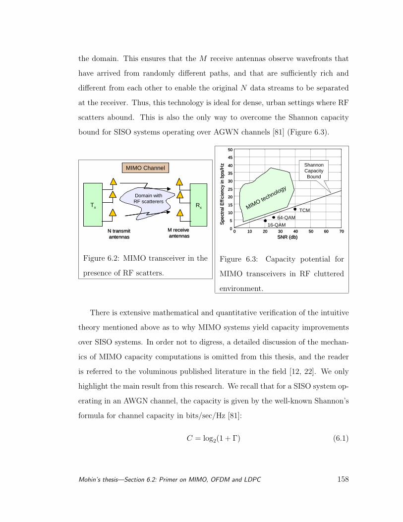
the domain. This ensures that the M receive antennas observe wavefronts that

have arrived from randomly different paths, and that are sufficiently rich and

different from each other to enable the original N data streams to be separated

at the receiver. Thus, this technology is ideal for dense, urban settings where RF

scatters abound. This is also the only way to overcome the Shannon capacity

bound for SISO systems operating over AGWN channels [81] (Figure 6.3).

MIMO Channel

Tx Rx

N transmitantennas

M receiveantennas

Domain with RF scatterers

MIMO Channel

Tx Rx

N transmitantennas

M receiveantennas

Domain with RF scatterers

Figure 6.2: MIMO transceiver in the

presence of RF scatters.

0 10 20 30 40 50 60 700

5

10

15

20

25

30

35

40

45

50

Spe

ctra

l Eff

icie

ncy

in b

ps/H

z

SNR (db)

Shannon Capacity Bound

MIMO technology

16-QAM

64-QAM

TCM

0 10 20 30 40 50 60 700

5

10

15

20

25

30

35

40

45

50

Spe

ctra

l Eff

icie

ncy

in b

ps/H

z

SNR (db)

Shannon Capacity Bound

MIMO technology

16-QAM

64-QAM

TCM

Figure 6.3: Capacity potential for

MIMO transceivers in RF cluttered

environment.

There is extensive mathematical and quantitative verification of the intuitive

theory mentioned above as to why MIMO systems yield capacity improvements

over SISO systems. In order not to digress, a detailed discussion of the mechan-

ics of MIMO capacity computations is omitted from this thesis, and the reader

is referred to the voluminous published literature in the field [12, 22]. We only

highlight the main result from this research. We recall that for a SISO system op-

erating in an AWGN channel, the capacity is given by the well-known Shannon’s

formula for channel capacity in bits/sec/Hz [81]:

C = log2(1 + Γ) (6.1)


where Γ is the signal to noise ratio. However, in a MIMO system with N transmit

and M receive antennas, the capacity increases to:

CMN = log2 det

(IN +

Γ

NHH∗

)(6.2)

= log2 det

(IM +

Γ

NH∗H

)(6.3)

=N∑

i=1

log2

(1 +

Γ

Nλi

)(6.4)

where H is the M ×N channel propagation (mixing) matrix (discussed in further

detail in Section 6.3), λi are the eigenvalues of the M × M matrix HH∗, I is

the identity matrix, and det(A) is the determinant of matrix A. We note that

the capacity of an M ×N system is the same as an N ×M and, therefore, this

expression be used for overloaded arrays where there are fewer receiving antennas

than transmitting antennas. For symmetric systems with M = N , the capacity

is thus a function of N , the SNR, and the eigenvalues λi.

If the propagation is line of sight (LOS) and there is little or no multipath,

then the majority of the eigenvalues λi will be insignificant. In the limiting

case of one dominant eigenvalue, the MIMO capacity expression simplifies to the

following lower bound:

CminNN = log2(1 + NΓ) (6.5)

which represents the case when there is maximum correlation between the receiv-

ing antennas and H has only a single degree of freedom. In this case, the capacity

increases only logarithmically with the number of antennas.

However, if the domain of the MIMO system has many scattering surfaces,

then many multipath components are generated as a result and the receiving

antennas observe signals from many different angles. In this case, upto N of the

eigenvalues λi can be significant, and the channel matrix H can have upto N


degrees of freedom. The correlation between the receiving antennas is thus low.

In the limit, if H is an orthogonal matrix with HH∗ being the identity matrix,

then all the N eigenvalues are equal to N , and the resulting upper bound on

capacity is given by:

CmaxNN = N log2(1 + Γ) (6.6)

So, for multipath rich environments, the theoretical limiting MIMO capacity

increases linearly with the number of antennas (while the total amount of trans-

mitter power is fixed and divided equally among the transmitting antennas).

This is the fundamental motivation that for using a MIMO based system for our

proposed transceiver.

6.2.2 Orthogonal Frequency Domain Multiplexing (OFDM)

As mentioned earlier, the mobile radio channel is characterized by multipath fad-

ing environment. The signal at the receiver contains a large number of reflected

radio waves that arrive at the receiver at different times. However, for broad-

band multimedia mobile communication systems, it is nowadays necessary to use

high-bit-rate transmission of at least several megabits per second. Unfortunately,

if digital data is transmitted at this rate, the delay time of the reflected, delayed

waves exceeds 1 symbol time for most urban settings. These reflected waves in-

terfere with the direct line of sight reception (if there is one) and causes ISI, or

frequency selective fading. Such frequency-selective fading is a dominant impair-

ment in mobile communications. Fading reduces receive signal-to-noise ratio and

degrades the bit-error-rate (BER).

To combat frequency-selective fading, the effects of ISI must be eliminated.

There are several ways to accomplish this. Adaptive equalization techniques at

the receiver can be used, but in practice, achieving this equalization at several


megabits per second is difficult and expensive. The alternative technique is to use

multicarrier transmission techniques, in particular orthogonal frequency domain

multiplexing (OFDM) [4].

The basic idea of OFDM is to divide the available spectrum into several sub-

channels, and to transmit independent carriers in each subchannel. By making

all the subchannels narrowband, they experience almost flat fading, which makes

equalization unnecessary or very simple. However, if traditional “brick-wall” [74]

type filters are used to separate the subchannels, then there is considerable in-

efficiency in packing the subchannels, with their guard bands, into the available

bandwidth. Instead, to obtain high spectral efficiency, the frequency response of

the subchannels are chosen to be orthogonal so that they may overlap in the fre-

quency domain. Hence the name OFDM. The orthogonality is maintained even

when the composite signal passes through a time-dispersive channel by introduc-

ing a cyclic prefix.

The frequency domain overlapping is most easily accomplished by means of

digital signal processing techniques, specifically fast Fourier transforms (FFT)

and inverse FFTs, rather than by frequency synthesizers.1 So, if D0, D1, . . . , DN−1

are the data symbols, then the discrete Fourier transform (DFT) can be used as

a linear transformation to map the complex data symbols to OFDM symbols

d0, d1, . . . , dN−1 such that:

dk =N−1∑n=0

Dnej2πn kN (6.7)

1Incidentally, it is only recently that very fast FFT hardware processors that enable real-time OFDM operations have become widely available; and this is the primary reason whymulticarrier systems have gained in popularity.


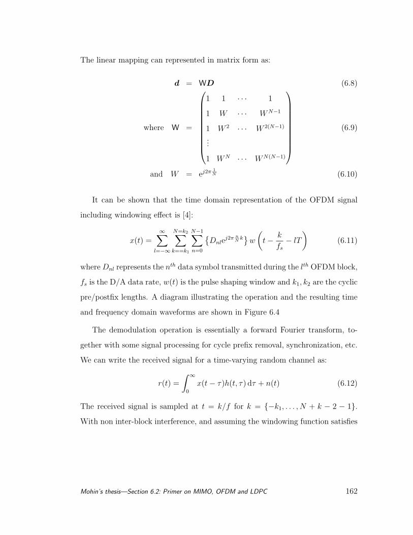
The linear mapping can represented in matrix form as:

d = WD (6.8)

where W =

1 1 · · · 1

1 W · · · WN−1

1 W 2 · · · W 2(N−1)

...

1 WN · · · WN(N−1)

(6.9)

and W = ej2π 1N (6.10)

It can be shown that the time domain representation of the OFDM signal

including windowing effect is [4]:

x(t) =∞∑

l=−∞

N=k2∑

k==k1

N−1∑n=0

Dnle

j2π nN

k

w

(t− k

fs

− lT

)(6.11)

where Dnl represents the nth data symbol transmitted during the lth OFDM block,

fs is the D/A data rate, w(t) is the pulse shaping window and k1, k2 are the cyclic

pre/postfix lengths. A diagram illustrating the operation and the resulting time

and frequency domain waveforms are shown in Figure 6.4

The demodulation operation is essentially a forward Fourier transform, to-

gether with some signal processing for cycle prefix removal, synchronization, etc.

We can write the received signal for a time-varying random channel as:

r(t) =

∫ ∞

0

x(t− τ)h(t, τ) dτ + n(t) (6.12)

The received signal is sampled at t = k/f for k = −k1, . . . , N + k − 2 − 1.With non inter-block interference, and assuming the windowing function satisfies


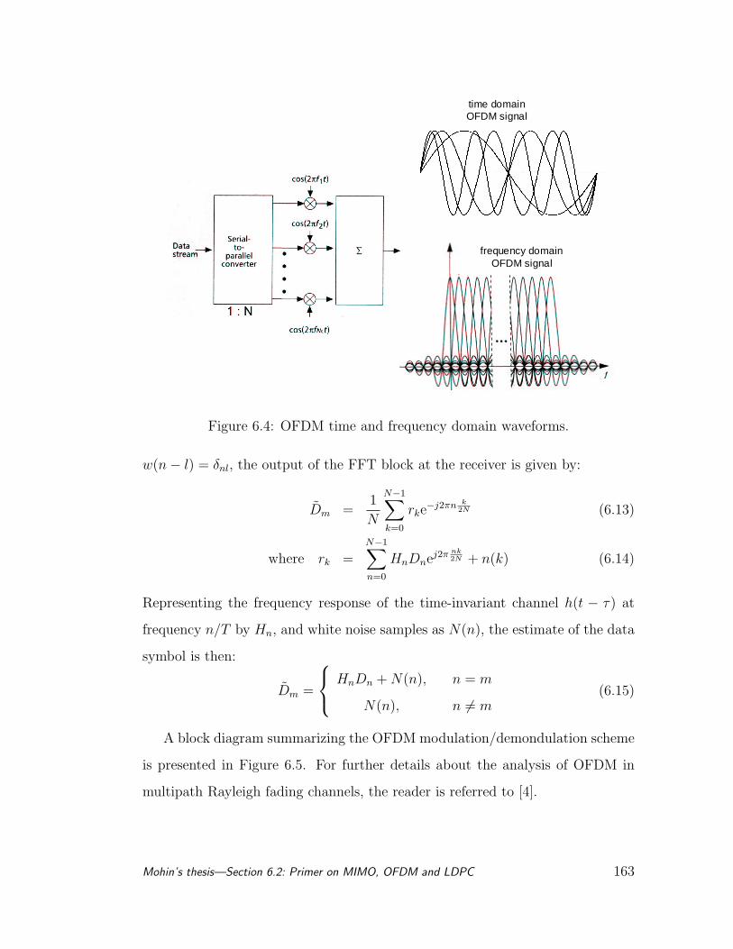
time domain OFDM signal

frequency domain OFDM signal

Figure 6.4: OFDM time and frequency domain waveforms.

w(n− l) = δnl, the output of the FFT block at the receiver is given by:

Dm =1

N

N−1∑

k=0

rke−j2πn k

2N (6.13)

where rk =N−1∑n=0

HnDnej2π nk2N + n(k) (6.14)

Representing the frequency response of the time-invariant channel h(t − τ) at

frequency n/T by Hn, and white noise samples as N(n), the estimate of the data

symbol is then:

Dm =

HnDn + N(n), n = m

N(n), n 6= m(6.15)

A block diagram summarizing the OFDM modulation/demondulation scheme

is presented in Figure 6.5. For further details about the analysis of OFDM in

multipath Rayleigh fading channels, the reader is referred to [4].


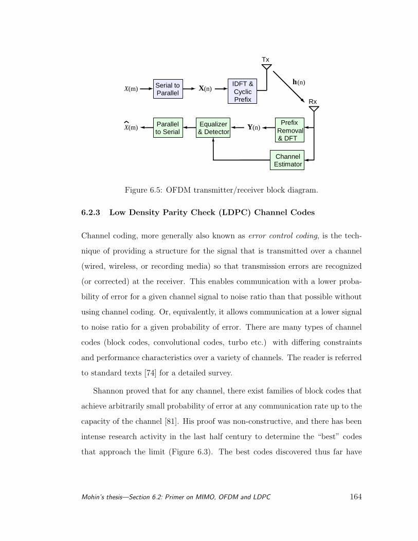
Serial to Parallel

Parallel to Serial

IDFT & Cyclic Prefix

Prefix Removal& DFT

X(m) X(n)

Equalizer & Detector

X(m)

Channel Estimator

Y(n)

Tx

Rx

h(n)

Figure 6.5: OFDM transmitter/receiver block diagram.

6.2.3 Low Density Parity Check (LDPC) Channel Codes

Channel coding, more generally also known as error control coding, is the tech-

nique of providing a structure for the signal that is transmitted over a channel

(wired, wireless, or recording media) so that transmission errors are recognized

(or corrected) at the receiver. This enables communication with a lower proba-

bility of error for a given channel signal to noise ratio than that possible without

using channel coding. Or, equivalently, it allows communication at a lower signal

to noise ratio for a given probability of error. There are many types of channel

codes (block codes, convolutional codes, turbo etc.) with differing constraints

and performance characteristics over a variety of channels. The reader is referred

to standard texts [74] for a detailed survey.

Shannon proved that for any channel, there exist families of block codes that

achieve arbitrarily small probability of error at any communication rate up to the

capacity of the channel [81]. His proof was non-constructive, and there has been

intense research activity in the last half century to determine the “best” codes

that approach the limit (Figure 6.3). The best codes discovered thus far have


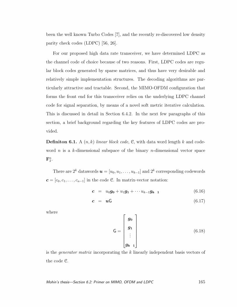
been the well known Turbo Codes [7], and the recently re-discovered low density

parity check codes (LDPC) [56, 26].

For our proposed high data rate transceiver, we have determined LDPC as

the channel code of choice because of two reasons. First, LDPC codes are regu-

lar block codes generated by sparse matrices, and thus have very desirable and

relatively simple implementation structures. The decoding algorithms are par-

ticularly attractive and tractable. Second, the MIMO-OFDM configuration that

forms the front end for this transceiver relies on the underlying LDPC channel

code for signal separation, by means of a novel soft metric iterative calculation.

This is discussed in detail in Section 6.4.2. In the next few paragraphs of this

section, a brief background regarding the key features of LDPC codes are pro-

vided.

Definiton 6.1. A (n, k) linear block code, C, with data word length k and code-

word n is a k-dimensional subspace of the binary n-dimensional vector space

Fn2 .

There are 2k datawords u = [u0, u1, . . . , uk−1] and 2k corresponding codewords

c = [c0, c1, . . . , cn−1] in the code C. In matrix-vector notation:

c = u0g0 + u1g1 + · · · uk−1gk1 (6.16)

c = uG (6.17)

where

G =

g0

g1

...

gk1

(6.18)

is the generator matrix incorporating the k linearly independent basis vectors of

the code C.


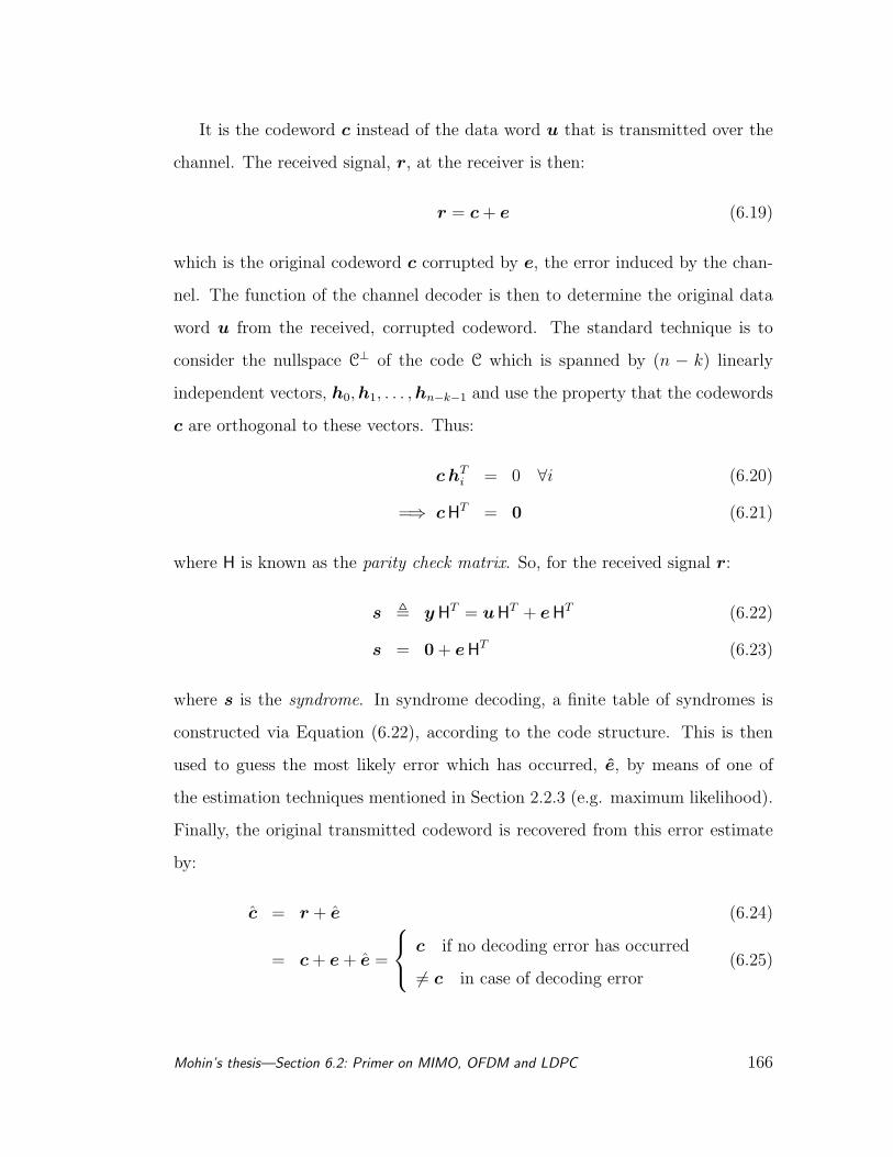
It is the codeword c instead of the data word u that is transmitted over the

channel. The received signal, r, at the receiver is then:

r = c + e (6.19)

which is the original codeword c corrupted by e, the error induced by the chan-

nel. The function of the channel decoder is then to determine the original data

word u from the received, corrupted codeword. The standard technique is to

consider the nullspace C⊥ of the code C which is spanned by (n − k) linearly

independent vectors, h0,h1, . . . , hn−k−1 and use the property that the codewords

c are orthogonal to these vectors. Thus:

c hTi = 0 ∀i (6.20)

=⇒ c HT = 0 (6.21)

where H is known as the parity check matrix. So, for the received signal r:

s , y HT = u HT + e HT (6.22)

s = 0 + e HT (6.23)

where s is the syndrome. In syndrome decoding, a finite table of syndromes is

constructed via Equation (6.22), according to the code structure. This is then

used to guess the most likely error which has occurred, e, by means of one of

the estimation techniques mentioned in Section 2.2.3 (e.g. maximum likelihood).

Finally, the original transmitted codeword is recovered from this error estimate

by:

c = r + e (6.24)

= c + e + e =

c if no decoding error has occurred

6= c in case of decoding error(6.25)


which is successful in recovering the original codeword with a specified probability

of error, depending on the noise statistics and code design (G).

Definiton 6.2. A regular (n, k) LDPC code is a linear block code who’s parity

check matrix, H contains exactly wc 1’s per column and wr = wc · (n/m) 1’s per

row, where wc ¿ wm.

If the number of 1’s per column or row are not constant, then the code is

an irregular LDPC code. LDPC codes were invented by Gallager at MIT in the

1960’s [26], and rediscovered by Makcay in the 1990’s [56]. Since the generator

matrix (and hence the parity check matrix) is sparse, the minimum code distance,

dmin, which is the minimum number of columns of the parity check matrix that

adds up to 0, is large. This is precisely what gives LDPC codes the ability to

correct a large number of channel errors. Another interesting feature of LDPC

codes shown by Gallager is that over an ensemble of regular LDPC codes, the

distribution function for dmin for a randomly selected member of the ensemble re-

sembles a step function, for dmin, greater than a small threshold, δn, where δ is a

function of wc, wr. This implies that almost any randomly selected sparse gener-

ator matrix, G, for relatively large block lengths is automatically a “good” LDPC

code. This remarkable fact makes the design of LDPC codes straightforward.

For the LDPC code for our transceiver design, we simply used the semi-

random construction technique [56], whereby H is generated with weight-wc

columns, weight-wr rows, and no two columns are allowed to have an overlap

greater than one. In addition, short cycles are avoided and H = [H1...H2 con-

strained so that H2 is full rank. The algorithm is summarized as Algorithm 6.1.

Algorithm 6.1. Construction of LDPC Codes:

1. Chose parameters n, k, wc, wr and Lmin = minimum cycle length. H will


then be an m × n matrix (m = n − k) with wc 1’s per column and wr 1’s

per row.

2. Set column counter ic = 0

3. Generate a weight-wc column vector and place in column ic of the H matrix

that is being generated.

4. In the H matrix at this point, if the weight of each row is≤ Wr, if the overlap

between any two columns is ≤ 1, and if all the cycle lengths are ≥ Lmin,

then ic = ic + 1.

5. if ic = n, STOP; else goto 3.

Because the algorithm is semi-random, the algorithm may not converge all

the time. In such cases, it should be restarted with a new seed. A few extra

steps may be necessary to ensure that the row weights are uniformly equal to wr,

but this is usually unnecessary since irregular LDPC codes have been shown to

be better than regular LDPC codes. Once H is obtained, it is straightforward to

obtain the generator matrix, G and perform the codeword encoding operation:

c = u G.

The decoding algorithms for LDPC codes are elegant iterative techniques,

originally proposed by Gallager [26], and are effectively optimal. It iteratively

computes distributions of variables in graph-based models and come under dif-

ferent names, depending upon the context:

• sum-product algorithm (all graphical models)

• min-sum algorithm (approximation to the sum-product algorithm)

• forward-backward algorithm, BCJR algorithm, APP or MAP algorithm

(trellis-based graphical models)


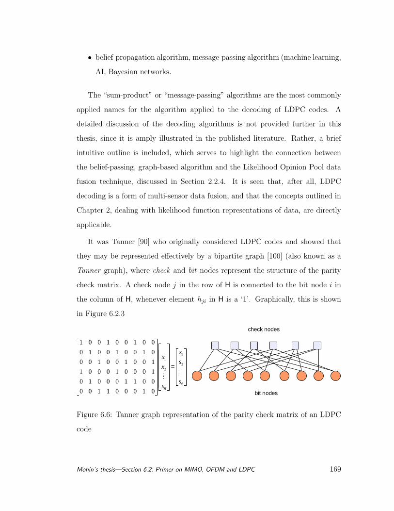
• belief-propagation algorithm, message-passing algorithm (machine learning,

AI, Bayesian networks.

The “sum-product” or “message-passing” algorithms are the most commonly

applied names for the algorithm applied to the decoding of LDPC codes. A

detailed discussion of the decoding algorithms is not provided further in this

thesis, since it is amply illustrated in the published literature. Rather, a brief

intuitive outline is included, which serves to highlight the connection between

the belief-passing, graph-based algorithm and the Likelihood Opinion Pool data

fusion technique, discussed in Section 2.2.4. It is seen that, after all, LDPC

decoding is a form of multi-sensor data fusion, and that the concepts outlined in

Chapter 2, dealing with likelihood function representations of data, are directly

applicable.

It was Tanner [90] who originally considered LDPC codes and showed that

they may be represented effectively by a bipartite graph [100] (also known as a

Tanner graph), where check and bit nodes represent the structure of the parity

check matrix. A check node j in the row of H is connected to the bit node i in

the column of H, whenever element hji in H is a ‘1’. Graphically, this is shown

in Figure 6.2.3

bit nodes

check nodes

11

22

69

1 0 0 1 0 0 1 0 0

0 1 0 0 1 0 0 1 0

0 0 1 0 0 1 0 0 1

1 0 0 0 1 0 0 0 1

0 1 0 0 0 1 1 0 0

0 0 1 1 0 0 0 1 0

sx

sx

sx

=

Figure 6.6: Tanner graph representation of the parity check matrix of an LDPC

code


During decoding, the received codeword is matched to the bit nodes, and the

structure of the parity check matrix then causes the check nodes to check the

parity of the resulting node connections from the check to the bit nodes. If the

parity of the connections at each check not does not match, it implies that the

received codeword is in error. In this case, the decoding algorithm then uses

bipartite graph and attempts to determine which of the bit nodes contain the

error. The check nodes provides “guesses” regarding which nodes it suspects

are in error (due to parity check failures) to the bit nodes. This is a form of

extrinsic information, and in the soft-decoding version of the algorithm, involves

likelihood ratios (similar to the observations of multiple sensors in a distributed

sensor network, Section 2.2.4), as in Equation (6.26).

Log-Likelihood Ratio (LRR) = log

Pr(ci = 0 | r, si)

Pr(ci = 1 | r, si)

(6.26)

where, r is the received codeword, si is the event that the bits in the codeword c

satisfy the wc parity check equations involving ci. In the second half of the itera-

tion, the aggregated likelihood metrics and messages from the bit nodes are then

passed back to the check nodes. Decoding is stopped after a maximum number

of iterations is reached or before that, provided c HT = 0, else the codeword error

in unrecoverable. The algorithm is summarized as Algorithm

Algorithm 6.2. General LDPC Decoding Algorithm:

1. Initialize bit/check nodes.

2. Pass messages from bit nodes to check nodes for parity check.

3. Pass messages (parity check likelihood ratios) from check nodes to bit nodes.

4. Find x and c from the probabilistic information residing at the nodes xi,attempting to satisfy c HT = 0 within a maximum number of iterations,

then goto 2; else STOP - declare error, goto 2.


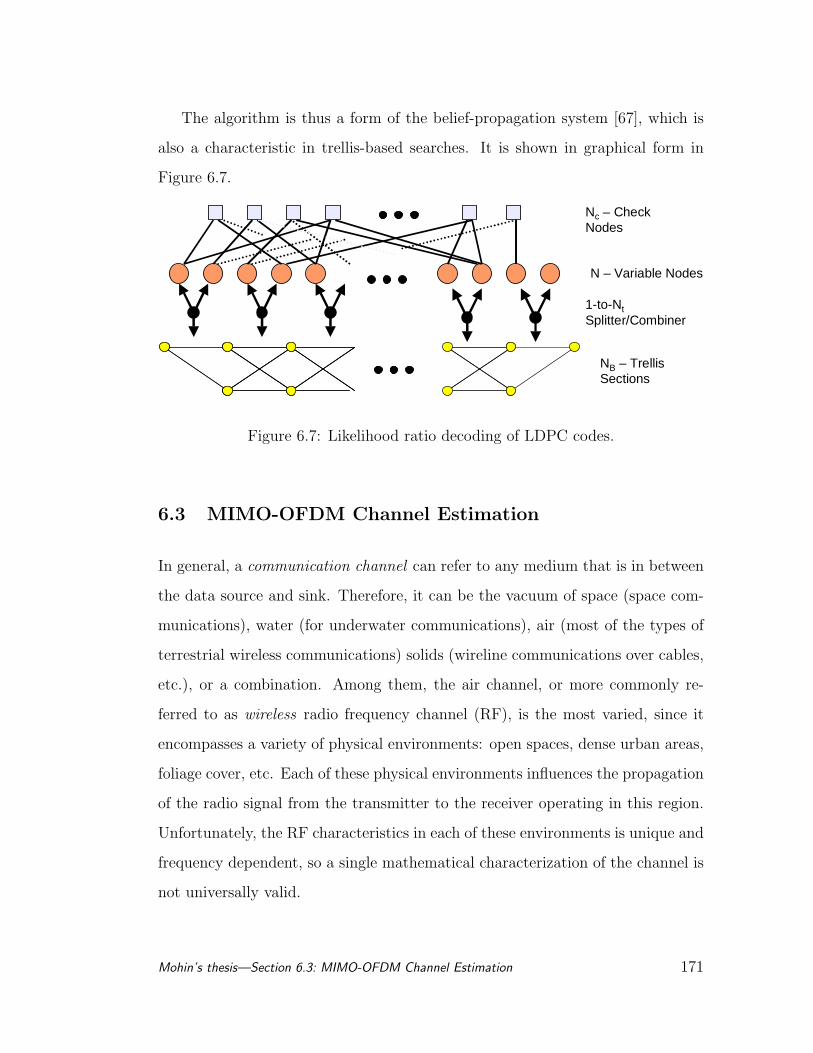
The algorithm is thus a form of the belief-propagation system [67], which is

also a characteristic in trellis-based searches. It is shown in graphical form in

Figure 6.7.

NB – Trellis Sections

N – Variable Nodes

Nc – Check Nodes

1-to-NtSplitter/Combiner

Figure 6.7: Likelihood ratio decoding of LDPC codes.

6.3 MIMO-OFDM Channel Estimation

In general, a communication channel can refer to any medium that is in between

the data source and sink. Therefore, it can be the vacuum of space (space com-

munications), water (for underwater communications), air (most of the types of

terrestrial wireless communications) solids (wireline communications over cables,

etc.), or a combination. Among them, the air channel, or more commonly re-

ferred to as wireless radio frequency channel (RF), is the most varied, since it

encompasses a variety of physical environments: open spaces, dense urban areas,

foliage cover, etc. Each of these physical environments influences the propagation

of the radio signal from the transmitter to the receiver operating in this region.

Unfortunately, the RF characteristics in each of these environments is unique and

frequency dependent, so a single mathematical characterization of the channel is

not universally valid.

Mohin’s thesis—Section 6.3: MIMO-OFDM Channel Estimation 171

The dense urban area, specifically, with multiple physical structures, RF re-

flecting/absorbing areas, and strong sources of interference, is a particularly harsh

RF environment. Also referred to as the mobile communication channel, this

channel is characterized as being the most difficult environment to conduct wire-

less communications over. Because of multiple signal reflections (and random

adding/subtracting of the resulting signal paths), this channel is prone to multi-

path fading, which takes the form of nonlinear channel responses in the frequency

spectrum.

To successfully design radio devices for the mobile RF channel (for detection,

demodulation, decoding), it is necessary to be able to estimate the effects of the

channel in the time/frequency domain. The estimation is, by definition, only an

approximation since the channel state is infinite dimensional. The traditional ap-

proach for single-input single-output systems (1 transmit and 1 receive antenna)

has been to be model the effects of the channel by means of a large finite-state

machine (FSM). The engineering version of this model is in the form of a Finite

Impulse Response (FIR) filter together with a AWGN source. The filter’s impulse

response is then tuned to approximate the impulse response of the channel under

consideration, which corresponds to the noise contaminated multipath behavior

of the RF channel.

The magnitude, phase and time of arrival of the multipath components, in

particular, are the critical factors that are of importance to the radio designer.

The FIR structure can model these as a fractionally sampled filter approximat-

ing the discrete-time sampled version of the infinite-dimensional mobile channel.

The problem of estimating the channel parameters (channel estimation) then

simply reduces to estimating the time-varying FIR filter coefficients, and the de-

lay spacing of the taps. Thus, for a SISO system, the end result is a tapped delay


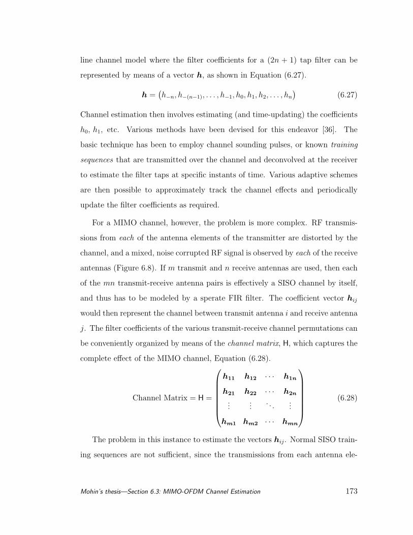
line channel model where the filter coefficients for a (2n + 1) tap filter can be

represented by means of a vector h, as shown in Equation (6.27).

h =(h−n, h−(n−1), . . . , h−1, h0, h1, h2, . . . , hn

)(6.27)

Channel estimation then involves estimating (and time-updating) the coefficients

h0, h1, etc. Various methods have been devised for this endeavor [36]. The

basic technique has been to employ channel sounding pulses, or known training

sequences that are transmitted over the channel and deconvolved at the receiver

to estimate the filter taps at specific instants of time. Various adaptive schemes

are then possible to approximately track the channel effects and periodically

update the filter coefficients as required.

For a MIMO channel, however, the problem is more complex. RF transmis-

sions from each of the antenna elements of the transmitter are distorted by the

channel, and a mixed, noise corrupted RF signal is observed by each of the receive

antennas (Figure 6.8). If m transmit and n receive antennas are used, then each

of the mn transmit-receive antenna pairs is effectively a SISO channel by itself,

and thus has to be modeled by a sperate FIR filter. The coefficient vector hij

would then represent the channel between transmit antenna i and receive antenna

j. The filter coefficients of the various transmit-receive channel permutations can

be conveniently organized by means of the channel matrix, H, which captures the

complete effect of the MIMO channel, Equation (6.28).

Channel Matrix = H =

h11 h12 · · · h1n

h21 h22 · · · h2n

......

. . ....

hm1 hm2 · · · hmn

(6.28)

The problem in this instance to estimate the vectors hij. Normal SISO train-

ing sequences are not sufficient, since the transmissions from each antenna ele-


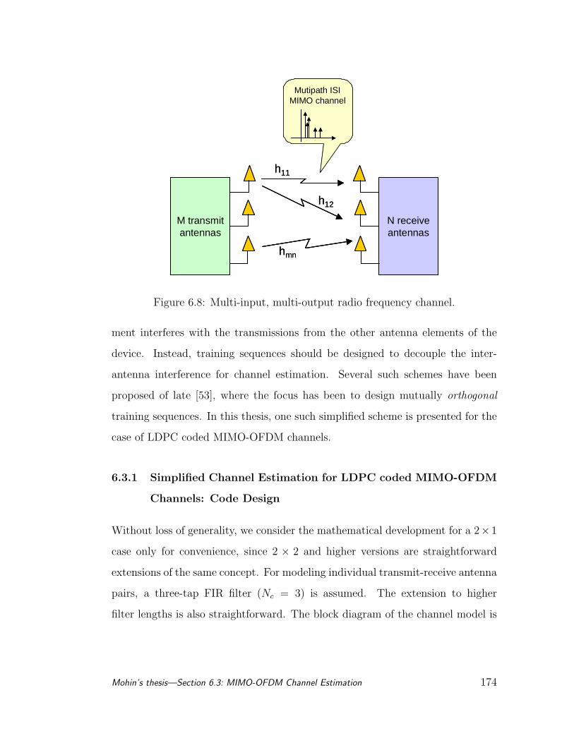
h11

M transmit antennas

N receive antennas

hmn

h12

Mutipath ISI MIMO channel

h11

M transmit antennas

N receive antennas

hmn

h12

Mutipath ISI MIMO channel

Figure 6.8: Multi-input, multi-output radio frequency channel.

ment interferes with the transmissions from the other antenna elements of the

device. Instead, training sequences should be designed to decouple the inter-

antenna interference for channel estimation. Several such schemes have been

proposed of late [53], where the focus has been to design mutually orthogonal

training sequences. In this thesis, one such simplified scheme is presented for the

case of LDPC coded MIMO-OFDM channels.

6.3.1 Simplified Channel Estimation for LDPC coded MIMO-OFDM

Channels: Code Design

Without loss of generality, we consider the mathematical development for a 2×1

case only for convenience, since 2 × 2 and higher versions are straightforward

extensions of the same concept. For modeling individual transmit-receive antenna

pairs, a three-tap FIR filter (Nc = 3) is assumed. The extension to higher

filter lengths is also straightforward. The block diagram of the channel model is


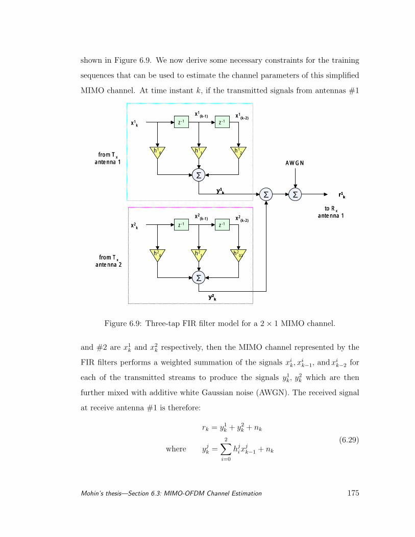
shown in Figure 6.9. We now derive some necessary constraints for the training

sequences that can be used to estimate the channel parameters of this simplified

MIMO channel. At time instant k, if the transmitted signals from antennas #1

z-1

Σ

h10 h1

1 h12

z-1

x1(k-1)

x1k

x1(k-2)

z-1

Σ

h20 h2

1 h202

z-1

x2(k-1)

x2k

x2(k-2)

Σ Σ

AWGN

y1k

y2k

r1k

from Txantenna 1

from Txantenna 2

to Rxantenna 1

z-1

Σ

h10 h1

1 h12

z-1

x1(k-1)

x1k

x1(k-2)

z-1

Σ

h20 h2

1 h202

z-1

x2(k-1)

x2k

x2(k-2)

Σ Σ

AWGN

y1k

y2k

r1k

from Txantenna 1

from Txantenna 2

to Rxantenna 1

Figure 6.9: Three-tap FIR filter model for a 2× 1 MIMO channel.

and #2 are x1k and x2

k respectively, then the MIMO channel represented by the

FIR filters performs a weighted summation of the signals xik, x

ik−1, and xi

k−2 for

each of the transmitted streams to produce the signals y1k, y2

k which are then

further mixed with additive white Gaussian noise (AWGN). The received signal

at receive antenna #1 is therefore:

rk = y1k + y2

k + nk

where yjk =

2∑i=0

hjix

jk−1 + nk

(6.29)


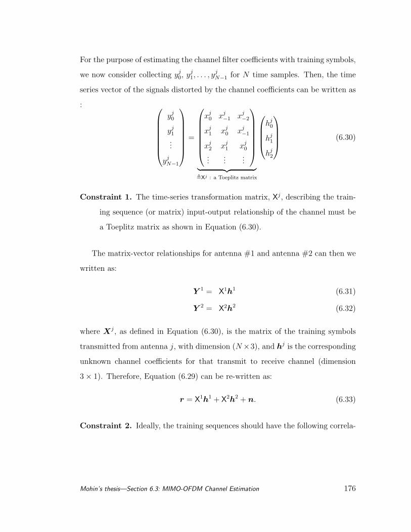
For the purpose of estimating the channel filter coefficients with training symbols,

we now consider collecting yj0, yj

1, . . . , yjN−1 for N time samples. Then, the time

series vector of the signals distorted by the channel coefficients can be written as

:

yj0

yj1

...

yjN−1

=

xj0 xj

−1 xj−2

xj1 xj

0 xj−1

xj2 xj

1 xj0

......

...

︸︷︷︸,Xj : a Toeplitz matrix

hj0

hj1

hj2

(6.30)

Constraint 1. The time-series transformation matrix, Xj, describing the train-

ing sequence (or matrix) input-output relationship of the channel must be

a Toeplitz matrix as shown in Equation (6.30).

The matrix-vector relationships for antenna #1 and antenna #2 can then we

written as:

Y 1 = X1h1 (6.31)

Y 2 = X2h2 (6.32)

where Xj, as defined in Equation (6.30), is the matrix of the training symbols

transmitted from antenna j, with dimension (N×3), and hj is the corresponding

unknown channel coefficients for that transmit to receive channel (dimension

3× 1). Therefore, Equation (6.29) can be re-written as:

r = X1h1 + X2h2 + n. (6.33)

Constraint 2. Ideally, the training sequences should have the following correla-


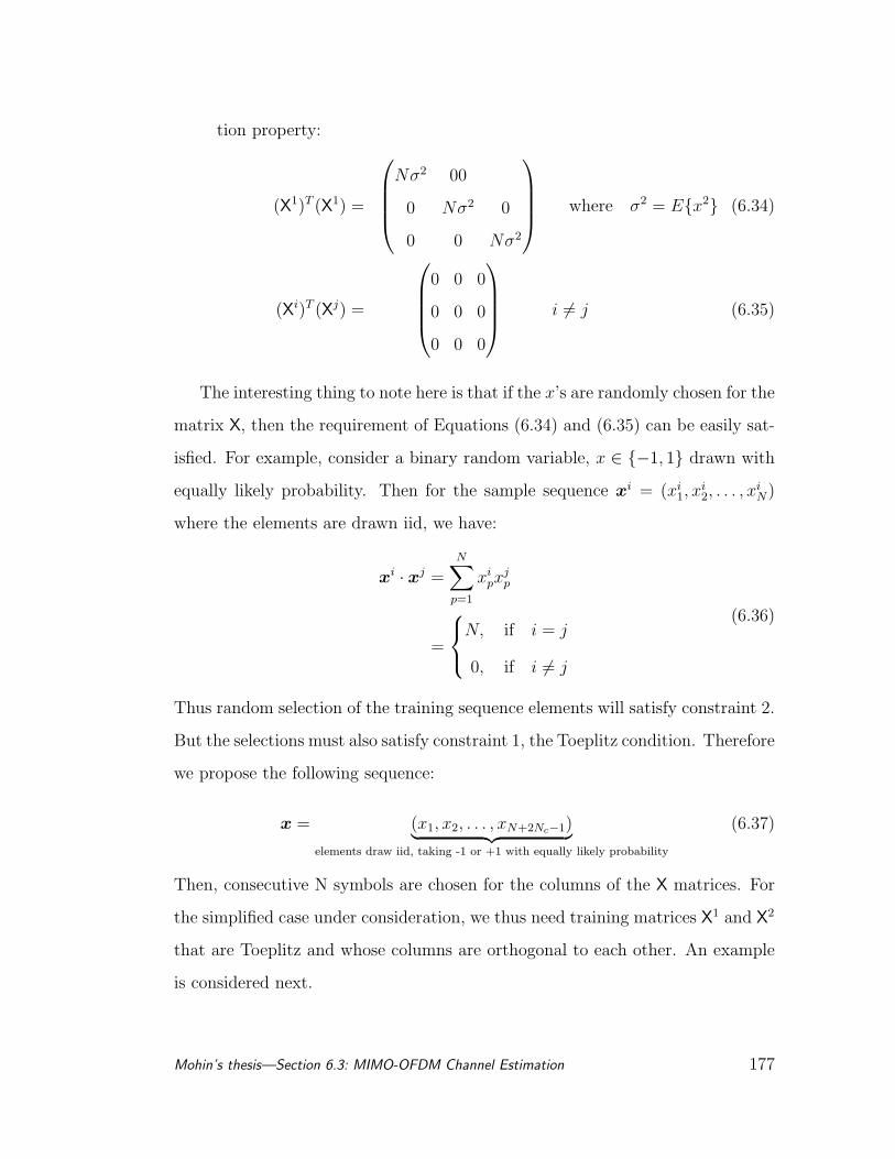
tion property:

(X1)T (X1) =

Nσ2 00

0 Nσ2 0

0 0 Nσ2

where σ2 = Ex2 (6.34)

(Xi)T (Xj) =

0 0 0

0 0 0

0 0 0

i 6= j (6.35)

The interesting thing to note here is that if the x’s are randomly chosen for the

matrix X, then the requirement of Equations (6.34) and (6.35) can be easily sat-

isfied. For example, consider a binary random variable, x ∈ −1, 1 drawn with

equally likely probability. Then for the sample sequence xi = (xi1, x

i2, . . . , x

iN)

where the elements are drawn iid, we have:

xi · xj =N∑

p=1

xipx

jp

=

N, if i = j

0, if i 6= j

(6.36)

Thus random selection of the training sequence elements will satisfy constraint 2.

But the selections must also satisfy constraint 1, the Toeplitz condition. Therefore

we propose the following sequence:

x = (x1, x2, . . . , xN+2Nc−1)︸︷︷︸elements draw iid, taking -1 or +1 with equally likely probability

(6.37)

Then, consecutive N symbols are chosen for the columns of the X matrices. For

the simplified case under consideration, we thus need training matrices X1 and X2

that are Toeplitz and whose columns are orthogonal to each other. An example

is considered next.


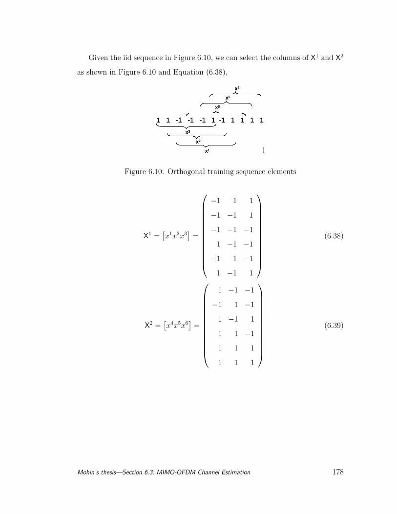
Given the iid sequence in Figure 6.10, we can select the columns of X1 and X2

as shown in Figure 6.10 and Equation (6.38),

1 1 -1 -1 -1 1 -1 1 1 1 1

x3

x2

x1

x6

x5

x4

1 1 -1 -1 -1 1 -1 1 1 1 1

x3x3

x2x2

x1x1

x6x6

x5x5

x4x4

l

Figure 6.10: Orthogonal training sequence elements

X1 =[x1x2x3

]=

−1 1 1

−1 −1 1

−1 −1 −1

1 −1 −1

−1 1 −1

1 −1 1

(6.38)

X2 =[x4x5x6

]=

1 −1 −1

−1 1 −1

1 −1 1

1 1 −1

1 1 1

1 1 1

(6.39)


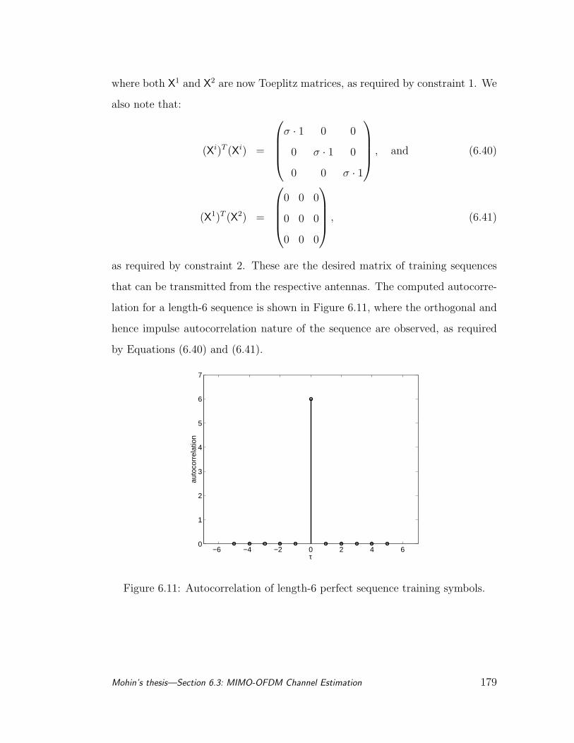
where both X1 and X2 are now Toeplitz matrices, as required by constraint 1. We

also note that:

(Xi)T (Xi) =

σ · 1 0 0

0 σ · 1 0

0 0 σ · 1

, and (6.40)

(X1)T (X2) =

0 0 0

0 0 0

0 0 0

, (6.41)

as required by constraint 2. These are the desired matrix of training sequences

that can be transmitted from the respective antennas. The computed autocorre-

lation for a length-6 sequence is shown in Figure 6.11, where the orthogonal and

hence impulse autocorrelation nature of the sequence are observed, as required

by Equations (6.40) and (6.41).

−6 −4 −2 0 2 4 60

1

2

3

4

5

6

7

τ

auto

corr

elat

ion

Figure 6.11: Autocorrelation of length-6 perfect sequence training symbols.


6.3.2 Channel Matrix Estimation

In the previous section, the matrices of the training sequences for each antenna

were designed. They were seen to be have desirable correlation properties and

a Toeplitz structure. At the receiving antenna(s), the individual channel para-

meters can then be estimated by the received versions of these training pulses,

as per the following theorem.

Theorem 6.1. The optimum estimate of the channel matrix hj for a MIMO

channel, given the training sequence matrices as in Equations (6.40) and (6.41),

is given by:

hj =[(Xj)T (Xj)

]−1(Xj)T r (6.42)

Proof. The total received signal for the 2× 1 system is given by:

r = X1h1 + X2h2 + n (6.43)

Therefore:

(X1)T r =[(X1)T (X1)

]h1 +

=0︷︸︸︷[(X1)T (X2)

]h2 +(X1)T n (6.44)

Thus, the Least Squares Estimate of h1, by the Gauss-Markov theorem [88], can

be shown to be:

h1 =[(X1)T (X1)

]−1(X1)T r (6.45)

A similar symmetric relationship holds for h2.

We note that the matrix[(X1)T (X1)

]is diagonal, so the estimation algorithm

can be efficiently implemented. The sequence in Figure 6.10 that we considered

for constructing the training matrix is a perfect sequence, and as we have seen,

it can be obtained by randomly selecting samples from binary random variables

∈ +1,−1.


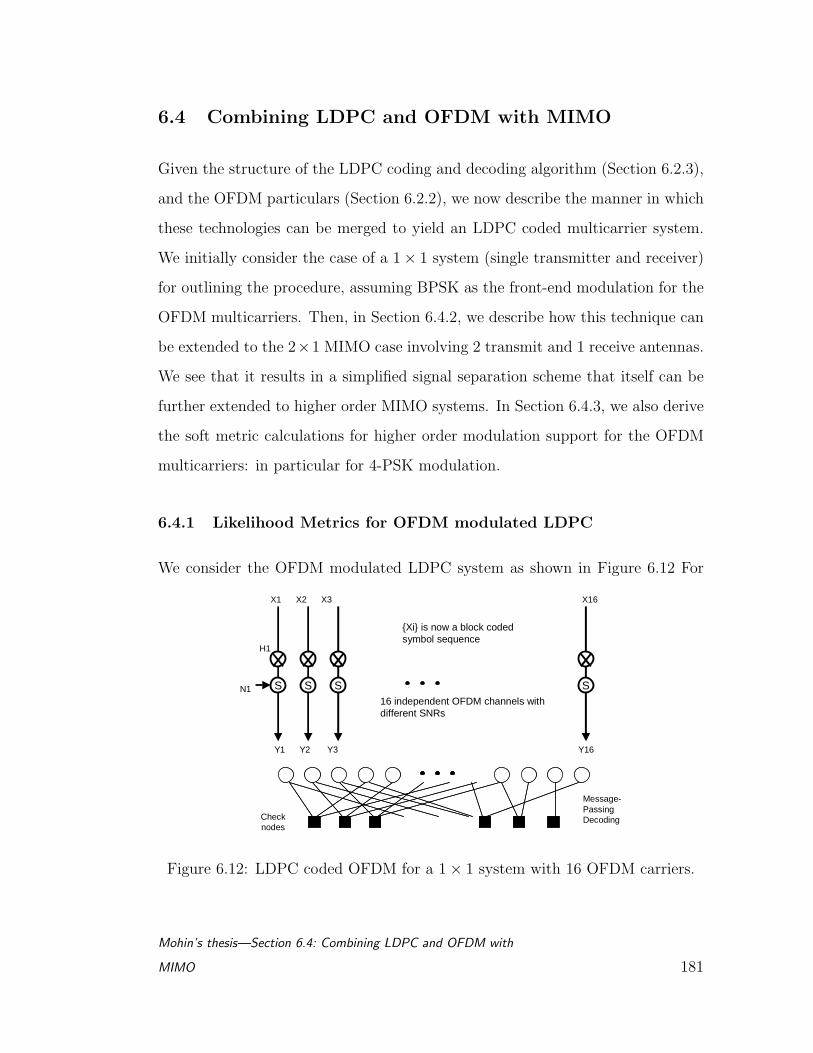
6.4 Combining LDPC and OFDM with MIMO

Given the structure of the LDPC coding and decoding algorithm (Section 6.2.3),

and the OFDM particulars (Section 6.2.2), we now describe the manner in which

these technologies can be merged to yield an LDPC coded multicarrier system.

We initially consider the case of a 1× 1 system (single transmitter and receiver)

for outlining the procedure, assuming BPSK as the front-end modulation for the

OFDM multicarriers. Then, in Section 6.4.2, we describe how this technique can

be extended to the 2×1 MIMO case involving 2 transmit and 1 receive antennas.

We see that it results in a simplified signal separation scheme that itself can be

further extended to higher order MIMO systems. In Section 6.4.3, we also derive

the soft metric calculations for higher order modulation support for the OFDM

multicarriers: in particular for 4-PSK modulation.

6.4.1 Likelihood Metrics for OFDM modulated LDPC

We consider the OFDM modulated LDPC system as shown in Figure 6.12 For

X1 X2 X3

SSSS

H1

N1

Y1 Y2 Y3 Y16

X16

16 independent OFDM channels with different SNRs

Message-PassingDecoding

Xi is now a block coded symbol sequence

Check nodes

Figure 6.12: LDPC coded OFDM for a 1× 1 system with 16 OFDM carriers.

Mohin’s thesis—Section 6.4: Combining LDPC and OFDM with

MIMO 181

this 1 × 1 system, in order to decode the LDPC channel code, we require a

suitable likelihood probability that can be used for the bit nodes of the LDPC

decoder. The result is stated as Theorem and derived below. We see that the

result turns out to be a relatively simple Gaussian dominated soft metric, if we

use the orthogonal bipolar symbolling scheme similar to the channel estimation

techniques discussed in Section 6.3. We assume that we have used the channel

estimation techniques described in that Section and thus have an estimate of the

channel matrix (in this case a vector of the channel coefficients, H).

Theorem 6.2. The optimum log-likelihood ratio soft metric for LDPC decoding

of an 1× 1 OFDM multicarrier system is:

1

σ2(hi + h∗i ) (6.46)

where hi is the channel coefficient for the ith individual OFDM carrier bin.

Proof. At the receiver of the system, we observe:

Yi︸︷︷︸observation

= hi︸︷︷︸known

· Xi︸︷︷︸unknown

+ Ni︸︷︷︸∼N(0,σ2)

(6.47)

Thus, the apriori probability yields:

Pr [Yi = y | Xi = x ∈ −1, +1] = Pr Ni = y − x (6.48)

=1√2πσ

· e−|y−hix|2

2σ2 (6.49)

from where the likelihood ratio can be computed to be:

Pr [Yi = y | Xi = 1]

Pr [Yi = y | Xi = −1]=

exp−y2−(hi+h∗i )+‖hi‖2

2σ2

exp−y2+(hi+h∗i )+‖hi‖2

2σ2

(6.50)

= exp

1

2σ2· 2(hi + h∗i )

(6.51)


MIMO 182

Taking logarithms:

log

Pr [Yi = y | Xi = 1]

Pr [Yi = y | Xi = −1]

=

1

σ2(hi + h∗i ) (6.52)

6.4.2 Signal Separation of LDPC coded OFDM Signals in MIMO Sys-

tems

The technique for combining the advantages of LDPC channel codes with the ISI-

combating OFDM multicarrier technology has been described for a 1 × 1 in the

previous subsection. However, a major problem occurs when trying to incorporate

the diversity benefits of a MIMO system on top of these techniques. This is the

issue of signal separation. For example, for a 2 MIMO system, both the transmit

antennas will be transmitting signals simultaneously (in the same time-frequency

dimension), so the receiver will observe a mixture of the two transmitted signals.

This is the same problem that we encountered in Section 6.3.1 when we were

attempting to estimate the MIMO channel parameters. However, in that case, we

designed known, special orthogonal training codes that could be easily separated.

For regular data transmissions, the symbols are unknown. What is required is

a technique that will enable the simultaneous transmission of independent data

streams on each of the MIMO antennas, and yet enable separation of the received,

mixed signals at the receiver.

There has been significant research activity in this area since the seminal

paper by Siavash Alamouti [1]. In the Alamouti scheme, a repetition coding

approach is taken for MIMO signal separation (for a 2×n system). In summary,

a symbol is first transmitted from one antenna, and the conjugate of the same

symbol is then re-transmitted from the second antenna, but with a unit delay.

The conjugate structure allows some selective processing at the receive antennas


MIMO 183

to eventually separate the transmitted streams. The Alamouti scheme is mainly

used to achieve transmit diversity of order 2, and thus reduces the probability of

error for the overall system. However, since the constraint length of the code is

only 2, it does not make a good code. Further work has extended the Alamouti

scheme to more than 2 transmit antennas. Our contention is that almost all of

the diversity benefits, together with added coding benefits can be achieved with

simple LDPC+OFDM embedded onto MIMO, since the LDPC code is a much

better code than a simple repetition code. In addition, the interference problem

can be solved with Turbo code-like iterations.

The proposed scheme is as follows (considered for a 2× 1 system). There are

two possible methods.

Method 1: Two streams of LDPC coded symbols are transmitted over the two

transmit antennas. For example, the odd indexed symbols can be transmitted via

the first antenna and the even indexed symbols can be transmitted over the second

antenna. The scheme can be extended in an analogous manner for more than 2

antenna systems. Considering the BPSK example discussed in previous sections,

if x1, x2, . . . , xN ∈ +1,−1, where N is the number of OFDM bins (e.g. 1024),

then x1, x3, x5, . . . would be transmitted from antenna 1, and x2, x4, x6, . . . from

antenna 2. At the receiver, the signals would mutually interfere, but the LDPC

code structure that the signals have been embedded with can now be exploited.

In principle, Baye’s rule can be applied to extract likelihood probabilities for the

odd and even sequences from the received signal rk = x1k + x2

k + n. The question

is in how to generate the likelihood probabilities for the even and odd sequences

in practice.

We propose that a simple scheme is to use the posterior probabilities from


MIMO 184

the odd sequence as the prior probability estimates for generating the likelihood

probability for the even sequence, and vice versa. In this manner, the LDPC de-

coding algorithm would thus be able to compute the forward-backward iterations

and separate the signal mixture into the even and odd streams.

Mathematically, we consider the first frequency bin (e.g. out of a total of 1024)

for the LDPC coded OFDM system. Then, rewriting Equation (6.33), we have:

r1 = H11x

11 + H2

1x21 + n1. (6.53)

We drop the subscripts indices for brevity. Then the likelihood metric for the

first antenna is given by:

Prr | x1 =∑

x2Prr, x2 | x1 (6.54)

=∑

x2Prr | x2,x1Prx2 | x1 (6.55)

=∑

x2Prr | x2,x1Prx2 (6.56)

since the odd and even streams x1, x2 are in general independent. The inter-

esting thing to note here is that Equation (6.56) is computable. The posterior

probability Prx2 | r over the whole sequence is used in place of Prx2, which

is obtained from a similar operation on the second antenna.

Finally, with the likelihood probability Prr | x1, the posterior probability

Prx1 | r itself can be obtained. This routine is then repeated at every iteration

for convergence to the correct estimate of the transmitted symbol.

Method 2: A variation on Method 1 can be achieved by sending two indepen-

dent blocks of LDPC codes over the two antennas. For example, if half of the

bits from an LDPC code word is transmitted on the first antenna then the other


MIMO 185

half can be sent on the second antenna, for an overall bit rate of 1 bps. The

advantage in this case is that the independence assumption of Equation (6.56) is

then perfectly valid. The same decoding scheme as discussed for Method 1 can

also be applied here, with an expectation of better convergence results.

We note that both these schemes are scalable to many transmit antennas. A

simulation study and results are presented in later sections of this chapter.

6.4.3 LDPC Soft Bit-Metrics for Decoding M-ary Symbols in OFDM

As mentioned earlier, the decoding development that has been considered in the

previous sections has been for the case of BPSK modulated OFDM carriers with

LDPC channel codes. In this scheme, the soft values of the transmitted bits

(not symbols), together with the likelihood values, are what are required to per-

form the forward-backward iterations for LDPC decoding (Section 6.2.3). In this

subsection, we now consider the case of LDPC decoding for OFDM with higher

constellation modulations, e.g 4-QAM or 16-QAM. Ostensibly, for 4-QAM, the

problem can be treated as two independent BPSK’s, but for the other constella-

tions, either a hard decision decoding can be performed (mapping the received

symbols to their guessed symbols and then LDPC decoding), or a soft decision

metric has to be derived. Hard decision decoding in this case is inherently a

poor choice since it can lead to instability in the forward-backward algorithm

and higher decoding errors. Thus, a soft decision metric is derived below.

We consider the case of the symbols being drawn from a 16-QAM signal

constellation. That is, Xk ∈ 16-QAM. Then there are four bits representing each

symbol in the constellation. For the symbol sequence X1, X2, . . . , XN , we need

to the extract the binary soft-decision metric for the bit sequence of length 4N .

For OFDM which produces no ISI, it is sufficient to show the procedure for a


MIMO 186

particular k ∈ 1, 2, . . . , N, since the operations are the same the for all k.

We have four bits per symbol, which are denoted by:

b1k, b

2k, b

3k and b4

k for each symbol Yk (6.57)

The received signal is Yk = Xk + Nk where Nk is AWGN and Xk ∈ 16-QAM. On

each Yk, we can generate 16 likelihood functions, which are basically 16 Gaussian

pdfs, each having a mean value of the 16 QAM symbols and a variance of σ2:

fk(i) = PrYk | Xk(i) = x(i) (6.58)

Alternatively, we can take the 15 ratios: f1/f1, f2/f1, . . . etc., all with respect

to f1 if we wish to avoid performing an exact calculation of the pdfs.

Next, the 16 QAM symbols in the constellation have to be mapped with a

specific rule to their 4 bit representations. It is an open question at this point

as to the optimum mapping rule (Gray code, anti-Gray code etc.) with respect

to LDPC decoding, but we have assumed the natural mapping rule assigning

symbol-indices to bits:

Xk(0) = (0000)

Xk(1) = (0001)

Xk(2) = (0010), etc. (6.59)

Denoting the posterior probability of the first bit being a “1” as π1k, we have:

π1k = Pr

b1k = 1 | Yk

(6.60)

There are 8 possibilities that the first bit is zero, i.e.(1 * * *), 23 = 8, so adding

all the 8 likelihoods and dividing out the sum of all the 16 likelihoods, we have:

π1k =

sum of the 8 likelihoods

sum of all the 16 likelihoods(6.61)


MIMO 187

The exact same routine holds for the other three positions of the “1”, such as

(* 1 * *), (* * 1 *), and (* * * 1), and symmetric expressions can be derived for

the other πik’s. These binary π’s are the required soft metrics that are then fed

to the LDPC decoding subroutine.

6.5 Adaptivity for LDPC coded MIMO-OFDM and Sys-

tem Design

One of the aims of this effort has been to enable the proposed transceiver system

to be adaptive to the channel and network conditions. If additional bandwidth be-

comes available, or SNR improves, etc., the radio units in communication should

be able to dynamically change their operating parameters to exploit the resource

that has become available. This is the basic concept behind software defined

radios [94].

Specifically, one parameter of frequent interest is frequency domain (spec-

trum) usage. For the proposed transceiver, this can be exploited by using an

adaptive form of OFDM, whereby the number of carriers are dynamically altered

in response to the available bandwidth. This is in response to studies that have

shown that a large portion of the bandwidth allocation for most types of networks

wireless services (with the possible exception of commercial cellular service) of-

ten remain idle. Examples include wireless LANs such as IEEE802.11a, military

radio systems, etc. This technology can attempt to fill those ‘frequency holes’ by

using multi-carrier modulation with a variable number of carriers. An example

for the IEEE802.11a standard is shown in Figure 6.13.

However, the adaptivity operation requires a feedback mechanism from the re-

ceiver to transmitter over a common control channel that relays updated channel

Mohin’s thesis—Section 6.5: Adaptivity for LDPC coded

MIMO-OFDM and System Design 188

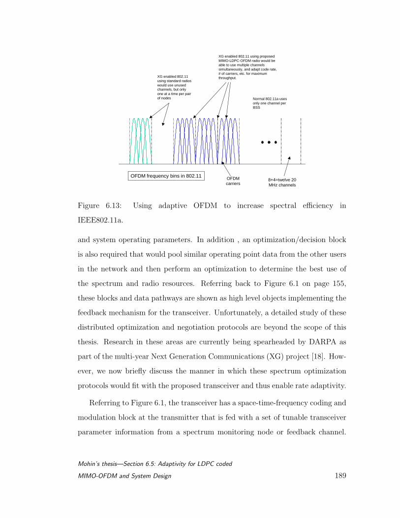
OFDM frequency bins in 802.11

Normal 802.11a uses only one channel per BSS

8+4=twelve 20 MHz channels

OFDM carriers

XG enabled 802.11 using standard radios would use unused channels, but only one at a time per pair of nodes

XG enabled 802.11 using proposed MIMO-LDPC-OFDM radio would be able to use multiple channels simultaneously, and adapt code rate, # of carriers, etc. for maximum throughput.

Figure 6.13: Using adaptive OFDM to increase spectral efficiency in

IEEE802.11a.

and system operating parameters. In addition , an optimization/decision block

is also required that would pool similar operating point data from the other users

in the network and then perform an optimization to determine the best use of

the spectrum and radio resources. Referring back to Figure 6.1 on page 155,

these blocks and data pathways are shown as high level objects implementing the

feedback mechanism for the transceiver. Unfortunately, a detailed study of these

distributed optimization and negotiation protocols are beyond the scope of this

thesis. Research in these areas are currently being spearheaded by DARPA as

part of the multi-year Next Generation Communications (XG) project [18]. How-

ever, we now briefly discuss the manner in which these spectrum optimization

protocols would fit with the proposed transceiver and thus enable rate adaptivity.

Referring to Figure 6.1, the transceiver has a space-time-frequency coding and

modulation block at the transmitter that is fed with a set of tunable transceiver

parameter information from a spectrum monitoring node or feedback channel.



The exact nature and availability of this channel would be application depen-

dent: e.g. it could be one of the 20 common channels for the IEEE 802.11a stan-

dard that is pre-negotiated. In this case, the modified 802.11a standard would

enable adaptive tuning of standard OFDM parameters. These parameters can

include the transmission bandwidth W, the carrier frequency fc, the number of

frequency bins Q, and the set of transmission rates Rii=1,...,Q in the individual

frequency bins fii=1,...,Q, which the spectrum monitoring/optimizing algorithm

has determined as being supportable for a given scenario. It should be noted that

in some frequency bins, the rate Ri can be selected to be zero, implying that no

information will be carried at those particular frequency locations. This would be

case if, in that portion of the RF spectrum, either there is on-going communica-

tions, or there is too much jamming-interference present. This ability of making

frequency-agile transmitted waveforms is one of the unique advantages of using

the OFDM modulation scheme which the proposed transceiver can exploits.

In addition, the transmission power and the number of bits per frequency

bin, can also be adaptively assigned, based on the general principle of the classic

’water-filling’ solution in the frequency domain. This can be done in several

ways: by adjusting the code rate of the low-density parity check codes, or by

manipulating the constellation size for the encoded information that is mapped

to the OFDM modulation symbol sets. Finally, adaptivity can also be obtained by

controlling the individual data streams that are transmitted from the independent

antenna elements. Repetition coding techniques can be used, like the Alamouti

scheme [1] discussed in Section 6.4.2, or the novel signal separation scheme as

discussed in Section 6.4.2.

An implementation block diagram of the transmitter and receiver portions of

the radio, the data packet structure, and a plot of the performance simulated



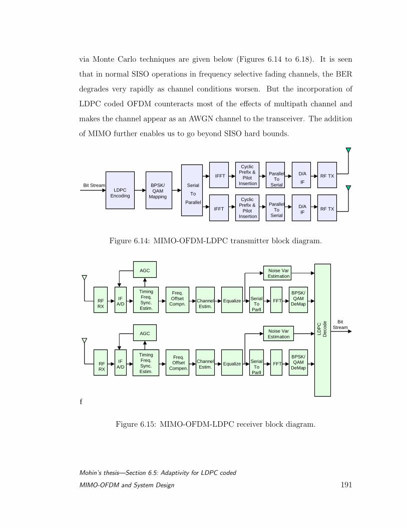
via Monte Carlo techniques are given below (Figures 6.14 to 6.18). It is seen

that in normal SISO operations in frequency selective fading channels, the BER

degrades very rapidly as channel conditions worsen. But the incorporation of

LDPC coded OFDM counteracts most of the effects of multipath channel and

makes the channel appear as an AWGN channel to the transceiver. The addition

of MIMO further enables us to go beyond SISO hard bounds.

LDPC Encoding

BPSK/QAM

Mapping

Serial

To

Parallel

Bit Stream

IFFT

IFFT

CyclicPrefix &

PilotInsertion

CyclicPrefix &

PilotInsertion

ParallelTo

Serial

ParallelTo

Serial

D/A

IF

D/AIF

RF TX

RF TX

Figure 6.14: MIMO-OFDM-LDPC transmitter block diagram.

f

IFA/D

Timing Freq.Sync.Estim.

Freq.Offset

Compn.Serial

ToParll

ChannelEstim.

Equalize FFT

AGC

IFA/D

Serial To

Parll

Equalize FFT

AGC Noise VarEstimation

RFRX

BitStream

Timing Freq.Sync.Estim.

Freq.Offset

Compen.

ChannelEstim.

Noise VarEstimation

BPSK/QAM

DeMap

BPSK/QAM

DeMap

RFRX

LDP

CD

ecod

e

Figure 6.15: MIMO-OFDM-LDPC receiver block diagram.



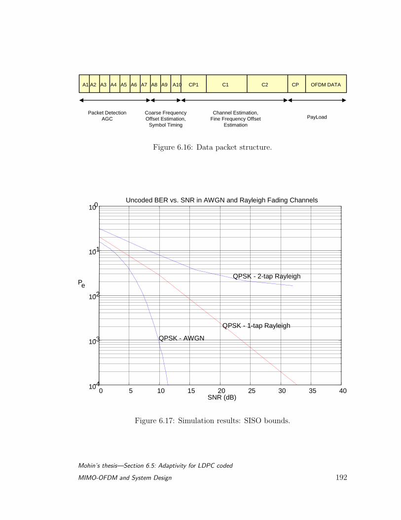
A1 A2 A3 A4 A5 A6 A7 A8 A9 A10 CP1 C1 C2 CP OFDM DATA

Coarse FrequencyOffset Estimation,

Symbol Timing

Packet DetectionAGC

Channel Estimation,Fine Frequency Offset

Estimation

PayLoad

Figure 6.16: Data packet structure.

0 5 10 15 20 25 30 35 4010-4

10-3

10-2

10-1

100

SNR (dB)

Pe

Uncoded BER vs. SNR in AWGN and Rayleigh Fading Channels

QPSK - AWGN

QPSK - 1-tap Rayleigh

QPSK - 2-tap Rayleigh

Figure 6.17: Simulation results: SISO bounds.



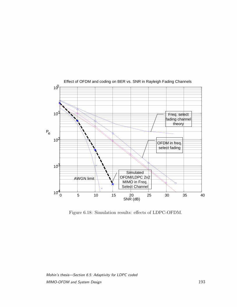
0 5 10 15 20 25 30 35 4010-4

10-3

10-2

10-1

100

SNR (dB)

Pe

Effect of OFDM and coding on BER vs. SNR in Rayleigh Fading Channels

AWGN limit

Simulated OFDM/LDPC 2x2

MIMO in Freq. Select Channel

Freq. select fading channel

theory

OFDM in freq. select fading

Figure 6.18: Simulation results: effects of LDPC-OFDM.



CHAPTER 7

Conclusion

This research effort has dealt with several inter-related problems relating to the

processing of information in wireless networks, and has presented a collection

of analysis, techniques and results designed to optimize performance in hybrid

networks. Sensors were used as the starting point of the study, and rules were

developed for a unified, consistent and efficient data fusion methodology, in het-

erogeneous, decentralized settings. The need for fundamental limits on perfor-

mance in such networks was realized, and some bounds on the data rate and de-

lay in idealized configurations were derived. Next, some practical issues dealing

with the administration of wireless resources, for sensor networking, for example,

was studied. In particular, a hybrid structure for connectivity among disparate,

heterogeneous wireless nodes was presented, and optimization techniques were

developed for efficient network performance under a variety of constraints. The

dependability of such networks was also analyzed, and protocols that improved

the dependability of the network were presented. Finally, bandwidth efficient

techniques based on the latest developments in digital communication theory

were proposed, that were able to achieve maximum spectral efficiency for node

to node communications in the decentralized network.

The overall unifying objective that is common to these topics is the analysis

of factors that affect performance when scaling the number of nodes in a sensor

system from a few (when combinatorial methods for system performance may be

194

tractable) to many (when statistical methods are the only options). The goal is to

determine intelligent unifying techniques from these varying analysis viewpoints,

which can be applied to quantify and answer some of the basic performance limits

questions for distributed sensing systems. In this regard, we believe this study

is novel, and yields insights into the many facets of design for heterogeneous

scalable, networked systems.

7.1 Future Directions

Several topics of further research and development, in each of the topics discussed

in this thesis, can be gleaned from the work that has been completed to date. The

broad goal will be as before: the development of tractable theoretical, modeling

and simulation tools that can assist in the ‘best-case’ design and deployment of

heterogeneous networked systems for particular mission objectives.

In the case of data fusion techniques, the Bayesian approach was seen as

the central unifying tool. However, it may be mentioned at this stage that the

basic philosophy behind the Bayesian probabilistic paradigm is not universally

accepted, and there exists alternative theories for decision making. Two of these

alternatives are possibility theory, also known as fuzzy logic, and Dempster-Schafer

theory [99]. Both have reached a level of maturity and a measure of success to

warrant their comparisons with the historically older probability theory. Such

a comparative analysis is likely to be very useful for distributed information

processing applications, such as sensor networking. It will yield invaluable insight

as to the utility of the various methods in application specific cases, and may

suggest ways to combine the methods and design hybrid techniques that can

extract the benefit from all the tools that are avaialable to the system designer.

Mohin’s thesis—Section 7.1: Future Directions 195

In the case of information theoretic bounds for sensor networks, many unan-

swered questions remain, unfortunately. The n-helper type bounds for non-

Gaussian channels is of immediate interest, as is the case when the nodes are

mobile. The development of the actual data compression and channel codes for

these distributed, cooperating sensor platforms is another huge area of practical

interest. It is not at all clear if the codes that have currently been developed

and optimized for SISO systems are in fact the optimum choice for distributed,

cooperating systems that can tolerate distortions. A thorough analytical and

simulation study is desired to determine the tradeoff parameters and performance

region. The general problem of satisfactorily combining networking and informa-

tion theory is also a major unsolved area of research [19]. Delay bounds, similar

to those calculated in Chapter 3, are required for practical sized networks with

real queueing models. They also have to be derived for the mobile cases, which

is where the QoS issues are of real concern.

For hybrid networks, there are a plethora of issues to be solved to enable true

wireless connectivity, “anywhere, anytime.” The approach taken in Chapter 4 is

not the only option that researchers have considered. A comprehensive end-to-

end system simulation study is necessary to weigh the relative merits of gateway

centric approaches, as opposed to completely ad hoc or “random” schemes. Mo-

bile wireless standards are still contentious issues, both commercially and from an

academic point of view, and it would be most helpful to have a unifying analytical

framework with which to analyze competing standards exhaustively. Needless to

say, many higher layer protocol issues are still major driving forces in the wireless

communications and networking community.

Reliability and dependability issues for ad hoc wireless nodes and networks,

as discussed in Chapter 5, unfortunately, are still under-appreciated topics, often


coming as after-thoughts to the main network design. At best, the attitude that

prevails is for enabling routing, MAC and other protocols to recover once failures

have occurred (link breakages, node failures, etc.), and not necessarily designing

networks that are fault tolerant and very reliable to begin with. A lack of usable

analytical and computational/predictive tools and techniques are primarily to

blame, and this thesis has attempted to address this shortcoming. Further work

remains to be done to enable more comprehensive techniques that are applicable

to real network systems, such as being able to incorporate protocol specific metrics

for the various network stack operations. A modular approach, as is the case for

cellular telephony systems, is called for. As mentioned in Chapter 5, the problems

may turn out to be intractable from a theoretical or computational complexity

point of view, but engineering approximations should be feasible in most cases of

practical interest.

Finally, bandwidth efficient MIMO techniques are an exciting new arena in

digital communications research. Its potential for precipitating a revolution in

sensor networking cannot be underestimated. Especially in tactical and military

applications, high data rate sensing/processing capabilities have become the cen-

tral focus and of prime importance for enabling network centric and operational

theater visualization applications. As illustrated in Chapter 6, software adaptive

radios that can efficiently utilize the time-frequency-space dimensions are the

current design challenges, and streamlined design/evaluation specifications are

desired. Despite large theoretical hurdles (unified LDPC decoding characteriza-

tion, efficient MIMO signalling techniques, joint source/channel coding for MIMO

systems etc.), rapid progress is being made. Unfortunately, commercial interest

has not yet caught on which has hindered the development of practical systems.

Actual results from prototypes and field measurements are lacking, which may

invalidate some cherished assumptions that many of use take for granted in the


design and simulation of these types of systems during pen and paper or soft-

ware development (e.g. accurate MIMO channel models, frequency compensation

performance for high data rate OFDM, true effect of mobility on MIMO perfor-

mance, etc.). Also, comprehensive comparative evaluations of the many proposed

schemes for OFDM and LDPC, and combinations thereof, are few. Work remains

in this regard.

It is heartening to note, however, that the recent progress and projected ad-

vances in semiconductor technology, nano-electronics, wireless communications

and system design tools are remarkable. These will no doubt enable the practical

development, deployment and use, on a mass scale, of the types of wireless dis-

tributed information processing systems that this thesis is about. New questions

and issues will inevitably arise. But, by necessity, the research questions of today

will be tackled and hopefully lead to the solutions of tomorrow, and make the

goal of ubiquitous wireless connectivity a reality.


References

[1] S. M. Alamouti, “A simple transmit diversity technique for wireless com-munications,” IEEE Journal on Selected Areas in Communications, vol. 16,no. 8, pp. 1451–1458, October 1998.

[2] K. Amouris et al., “A position-based multi-zone routing protocol for widearea mobile ad hoc networks,” in Proceedings of the 49th IEEE VehicularTechnology Conference, vol. 2, 1999, pp. 1365–1369.

[3] V. Anantharam and S. Verdu, “Bits through queues,” IEEE Transactionson Information Theory, vol. 42, no. 1, January 1996.

[4] A. R. S. Bahai and B. R. Saltzberg, Multi-Carrier Digital Communications:Theory and Applications of OFDM, ser. Information Technology: Transmis-sion, Processing, and Storage. New York, N.Y.: Kluwer Academic/PlenumPublishers, 1999.

[5] J. Balchen et al., Highly Redundant Sensing in Robotic Systems, ser. NATOAdvanced Science Institutes Series. Springer-Verlag, 1991, vol. 58, ch.Structural Solution of Highly Redundant Sensing in Robotic Systems.

[6] T. Berger et al., “Model distribution in decentralized multi-sensor fusion,”in Proceedings of the American Control Conference (ACC), 1991, pp. 2291–2294.

[7] C. Berrou and A. Galvieux, “Near optimum error correcting coding anddecoding: Turbo-codes,” IEEE Transactions on Communications, vol. 44,pp. 1261–1271, October 1996.

[8] D. Bertsekas, Nonlinear Programming. Belmont, Massachusetts: AthenaScientific, 1995.

[9] D. J. Bertsimas and J. N. Tsitsiklis, Introduction to Linear Optimization.Belmont, Massachusetts: Athena Scientific, 1997.

[10] W. L. Brogan, Modern Control Theory, 3rd ed. Englewood Cliffs, NewJersey: Prentice-Hall, 1991.

[11] D. Catlin, Estimation, Control and the Discrete Kalman Filter. Springer-Verlag, 1989.

[12] R. S. Cheng and S. Verdu, “Gaussian multiaccess channels with isi: Capac-ity region and multiuser water-filling,” IEEE Transactions on InformationTheory, vol. 39, no. 3, pp. 773–785, May 1993.

199

[13] C. Colbourn, The Combinatorics of Network Reliability. Oxford UniversityPress, 1987.

[14] T. M. Cover and J. A. Thomas, Elements of Information Theory. Hoboken,New Jersey: Wiley-Interscience, 1991.

[15] R. L. Cruz, “A calculus for network delay, part I: Network elements in iso-lation,” IEEE Transactions on Information Theory, vol. 37, no. 1, January1991.

[16] ——, “A calculus for network delay, part II: Network analysis,” IEEETransactions on Information Theory, vol. 37, no. 1, January 1991.

[17] I. Csiszar and J. Korner, “Towards a general theory of source networks,”IEEE Transactions on Information Theory, vol. IT-26, pp. 155–165, 1980.

[18] D. A. R. P. A. DARPA, “Next generation communications XG initiative,”World Wide Web, http://www.darpa.mil/ato/programs/xg.htm, 2001.

[19] A. Ephremides and B. Hajek, “Information theory and communication net-works: An unconsummated union,” IEEE Transactions on InformationTheory, vol. 44, no. 6, October 1998.

[20] R. A. Fisher, “On the mathematical foundations of theoretical statistics,”Philosophical Transactions of the Royal Society of London, vol. Sec A, no.222, pp. 309–368, 1922.

[21] A. M. Flynn, “Combining ultra-sonic and infra-red sensors for mobile robotnavigation,” International Journal of Robotics Research, vol. 7, no. 5, pp.5–14, 1988.

[22] G. Foschini, “Layered space-time architecture for wireless communicationin a fading environment when using multi-element antennas,” Bell LabsTechnical Journal, vol. 1, no. 2, pp. 41–59, 1998.

[23] G. Foschini, G. D. Golden, R. A. Valenzuela, and P. W. Wolniansky, “Sim-plified processing for high spectral efficiency wireless communications em-ploying multi-element arrays,” IEEE Journal on Selected Areas in Commu-nications, vol. 17, no. 11, pp. 1841–52, November 1999.

[24] R. Frank, Understanding Smart Sensors. Norwood, MA: Artech House,2000.

[25] B. Fristedt and L. Gray, A Modern Approach to Probability Theory.Boston, MA: Birkhauser, 1997, vol. Probability and its Applications.

Mohin’s thesis—REFERENCES 200

[26] R. G. Gallager, Low Density Parity Check Codes. Cambridge, MA: MITPress, 1963, vol. Research Monograph Series, no. 21.

[27] ——, Information Theory and Reliable Communications. New York, NY:John Wiley & Sons, 1968.

[28] E. Gamal and T. M. Cover, “Multiple user information theory,” Proceedingsof the IEEE, vol. 68, pp. 1466–1483, 1980.

[29] T. Garvey et al., “Model distribution in decentralized multi-sensor fusion,”Proceedings of the American Control Conference, pp. 2291–2294, 1991.

[30] J. Gondzio, “Multiple centrality corrections in a primal-dual method forlinear programming,” Computational Optimization and Applications, vol. 6,pp. 137–156, 1996.

[31] P. Gupta and P. R. Kumar, “The capacity of wireless networks,” IEEETransactions on Information Theory, vol. 46, no. 2, March 2000.

[32] Z. Haas et al., “Guest editorial on wireless ad hoc networks,” IEEE Journalon Selected Areas in Communications, vol. 17, no. 8, 1999.

[33] T. S. Han, “Hypothesis testing with multi-terminal data compression,”IEEE Transactions on Information Theory, vol. IT-33, pp. 759–772,November 1987.

[34] T. S. Han and K. Kobayashi, “A unified achievable rate region for a gen-eral class of multi-terminal source coding systems,” IEEE Transactions onInformation Theory, vol. IT-26, pp. 277–288, May 1980.

[35] K. P. Hatzis et al., “Fundamental control algorithms in mobile networks,” inACM Symposium on Parallel Algorithms and Architectures, 1999, pp. 251–260. [Online]. Available: “url–citeseer.nj.nec.com/hatzis99fundamental.html˝

[36] S. S. Haykin, Adaptive Filter Theory, 4th ed. Upper Saddle River, NewJersey: Prentice-Hall, 2002.

[37] Y.-C. Hu and D. B. Johnson, “Caching strategies in on-demand routingprotocols for wireless ad hoc networks,” in Proceedings of the 6th AnnualIEEE/ACM International Conference on Mobile Computing and Network-ing (MOBICOM), August 2000, pp. 231–242.

[38] C. Intanagonwiwat and D. D. Lucia, “The sink-based anycast routing pro-tocol for ad hoc wireless sensor networks,” USC Information Sciences In-stitute, Tech. Rep. 99–698, 1999.


[39] Intel Corporation, World Wide Web, http://www.intel.com.

[40] D. S. Johnson, Algorithms and Complexity, ser. Handbook of TheoreticalComputer Science. Amsterdam: Elsevier Science Publishing Company,1990, vol. A, ch. A Catalog of Complexity Classes, pp. 67–161.

[41] D. B. Johnson and D. A. Maltz, “Dynamic source routing in ad hoc wirelessnetworks,” in Mobile Computing, T. Imielinski and H. Korth, Eds. KluwerAcademic/Plenum Publishers, 1996, ch. 5, pp. 153–181.

[42] R. E. Kalman, “A new approach to linear filtering and prediction prob-lems,” Transactions of the ASME Journal of Basic Engineering, vol. 82,no. D, pp. 34–35, 1969.

[43] G. Karumanchi et al., “Information dissemination in partitionable mobilead hoc networks,” in Proceedings of the 18th IEEE Symposium on ReliableDistributed Systems, 1998, pp. 4–13.

[44] Y.-B. Ko and N. H. Vaidya, “Using location information in wireless ad hocnetwork,” in Proceedings of the 49th IEEE Vehicular Technology Confer-ence, vol. 3, 1999, pp. 1952–1956.

[45] ——, “Anycasting and geocasting in mobile ad hoc networks,” Departmentof Computer Sciences, Texas A & M University, Tech. Rep. TR00-015, 2000.

[46] G. Kocza, Models & Algorithms for Automatic Reliability Assessment ofComplex Systems. Delft University Press, 1997.

[47] R. Kuc and Siegel, “Physically based simulation model for acoustic sensorrobot navigation,” IEEE Transactions on Pattern Analysis and MachineIntelligence, vol. 9, no. 6, pp. 766–778, 1987.

[48] A. D. Kucar, “Mobile radio—an overview,” IEEE Personal Communica-tions Magazine, pp. 72–85, Nov. 1991.

[49] L. Lamport, R. Shostak, and M. Pease, “The byzantine generals problem,”ACM Transactions on Programming, Language and Systems, vol. 4, no. 3,pp. 382–401, July 1982.

[50] L. M. Leemis, Reliability: Probabilistic Models and Statistical Methods. En-glewood Cliffs, New Jersey: Prentice-Hall, 1994.

[51] B. M. Leiner, “Goals and challenges of the DARPA GloMo program (GlobalMobile Information Systems),” IEEE Personal Communications Magazine,vol. 3, no. 6, pp. 34–43, December 1996.


[52] J. J. Leonard, “Directed sonar sensing for mobile robot navigation,” Ph.D.dissertation, University of Oxford, 1991.

[53] Y. G. Li, “Simplified channel estimaton for ofdm systems with multi-ple transmit antennas,” IEEE Transaction on Wireless Communications,vol. 1, no. 1, pp. 67–75, January 2002.

[54] I. Local and M. A. N. S. Committee, “Wireless lan medium access control(MAC) and physical layer (PHY) specifications, IEEE Std 802.11-1997,”IEEE, New York, Tech. Rep., 1997.

[55] R. Luo and M. Kay, “Multi-sensor integration and fusion in intelligentsystems,” IEEE Transactions on Systems Man and Cybernetics, vol. 19,no. 5, pp. 901–931, 1989.

[56] D. J. C. Mackay, “Good error-correcting codes based on very sparse matri-ces,” IEEE Transactions on Information Theory, vol. 45, no. 2, pp. 399–431,March 1999.

[57] N. Malpani, J. L. Welch, and N. H. Vaidya, “Leader election algorithms formobile ad hoc networks,” in Proceedings of the 4th international workshopon Discrete algorithms and methods for mobile computing and communica-tions, Boston, MA, August 2000, pp. 96–103.

[58] Mathematics and A. N. L. Computer Science Division, World Wide Web,http://www.mcs.anl.gov.

[59] S. Mehrotra, “On the implementation of a primal-dual interior pointmethod,” SIAM Journal on Optimization, vol. 2, pp. 575–601, 1992.

[60] D. Middleton, Statistical Communication Theory. McGraw-Hill, 1960.

[61] L. E. Miller, “Probability of a two-hop connection in a random mobile net-work,” John Hopkins University 2001 Conference on Information Sciencesand Systems, March 2001.

[62] A. Mitchie and J. K. Aggarwal, “Multiple sensor integration through imageprocessing: A review,” Optical Engineering, vol. 23, no. 2, 1986.

[63] Y. Nakamura, Data fusion ion Robotics and Machine Intelligence. Aca-demic Press, 1992, ch. Geometric Fusion: Minimizing Uncertainty EllipsoidVolumes.

[64] NASA Jet Propulsion Laboratory (JPL), World Wide Web, http://www.jpl.nasa.gov.


[65] E. Pagani and G. P. Rossi, “Reliable broadcast in mobile multihop packetnetworks,” in Mobile Computing and Networking, 1997, pp. 34–42.

[66] V. Park and M. Corson, “A highly adaptive distributed routing algorithmfor mobile wireless networks,” in IEEE Infocomm, 1997.

[67] J. Pearl, Probabilistic Reasoning in Intelligent Systems: Networks of Plau-sible Inference. Morgan Kaufmann, 1997.

[68] C. E. Perkins and P. Bhagwa, “Highly dynamic destination-sequenceddistance-vector routing (DSDV) for mobile computers,” in ACM SIG-COMM Conference on Communications Architectures, Protocols and Ap-plications, 1994, pp. 234–244.

[69] C. E. Perkins and E. M. Royer, “Ad-hoc on-demand distance vector rout-ing,” in Proceedings of the 2nd IEEE Workshop on Mobile Computing Sys-tems and Applications, New Orleans, Louisiana, Feb. 1999, pp. 90–100.

[70] H. V. Poor, An Introduction to Signal Detection and Estimation. NewYork, NY: Springer-Verlag, 1988.

[71] R. Popoli, “The sensor management imperative,” in Multi-Target Multi-Sensor Tracking, Y. Bar-Shalom, Ed. Artech House, 1992, pp. 325–392.

[72] G. Pottie, “Hierarchical information processing in distributed sensor net-works,” in IEEE International Symposium on Information Theory, Cam-bridge, MA, August 16-21 1998.

[73] G. Pottie et al., “Wireless sensor networks,” in Information Theory Work-shop Proceedings, Killamey, Ireland, June 22-26 1998.

[74] J. G. Proakis, Digital Communications. New York, NY: McGraw-Hill,2000.

[75] S. Rai and D. P. Agrawal, Eds., Distributed Computing Network Reliability.IEEE Computer Press, 1990.

[76] P. Rai-Choudhury, Ed., MEMS and MOEMS Technology and Applications.Society of Photo-optical Instrumentation Engineers, 2000.

[77] J. Raju and J. J. Garcia-Luna-Aceves, “A comparison of on-demand and ta-ble driven routing for ad-hoc wireless networks,” in Proceedings of theIEEEInternational Conference on Communications(ICC 2000), vol. 3, New Or-leans, Louisiana, June 2000, pp. 1702–1706.


[78] G. G. Roussas, A Course in Mathematical Statistics, 2nd ed. Burlington,MA: Harcourt/Academic Press, 1997.

[79] E. Royer and C.-K. Toh, “A review of current routing protocols for adhoc wireless networks,” IEEE Personal Communications Magazine, vol. 6,no. 2, pp. 46–55, April 1999.

[80] J. T. Scheick, Linear Algebra with Applications. New York, NY: McGraw-Hill, 1996.

[81] C. E. Shannon, “A mathematical theory of communication,” Bell SystemsTechnical Journal, vol. 27, pp. 279–423, 1948.

[82] D. R. Shier, Network Reliability and Algebraic Structures. New York, NY:Oxford University Press, 1991.

[83] S. Singh et al., “Power-aware routing in mobile ad hoc networks,” in Pro-ceedings of the 4th Annual IEEE/ACM International Conference on MobileComputing and Networking (MOBICOM), Dallas, TX, 1998, pp. 181–190.

[84] D. Slepian and J. K. Wolf, “Noiseless coding of correlated informationsources,” IEEE Transactions on Information Theory, vol. IT-19, pp. 471–480, July 1973.

[85] A. P. Snow, “A survivability metric for telecommunications: Insights andshorcomings,” in Proceedings of the Information Survivability Workshop.Los Alamitos, CA: IEEE CS Press, Oct. 1998.

[86] K. Sohrabi and G. Pottie, “Performance of a self-organizing algorithm forwireless ad-hoc sensor networks,” IEEE Vehicular Technology Conference,Fall 1999.

[87] K. Sohrabi, G. Pottie, et al., “Protocols for self-organization for a wirelesssensor network,” IEEE Personal Communications Magazine, pp. 6–17, Oct.2000.

[88] H. Stark and J. W. Woods, Probability, Random Processes, and EstimationTheory for Engineers, 2nd ed. Englewood Cliffs, New Jersey: Prentice-Hall, 1994.

[89] M. Stone, “The opinion pool,” The Annals of Statistics, vol. 32, pp. 1339–1342, 1961.

[90] R. M. Tanner, “A recursive approach to low complexity codes,” IEEETransactions on Information Theory, pp. 533–547, September 1981.


[91] I. E. Telatar and R. G. Gallagher, “Combining queuing theory with infor-mation theory for multiaccess,” IEEE Journal on Selected Areas in Com-munications, vol. 13, no. 6, August 1995.

[92] D. Tipper, S. Ramaswamy, and T. Dahlberg, “Pcs network survivability,”Proceedings of the Mobile and Wireless Communication Networks Confer-ence (MWCN), 1999 1999.

[93] J. N. Tsitsiklis, “On the complexity of decentralized decision-making anddetection problems,” IEEE Transactions on Automatic Control, vol. 30,no. 5, pp. 440–446, 1985.

[94] W. Tuttlebee, Ed., Software Defined Radio: Enabling Technologies. JohnWiley & Sons, 2002.

[95] USC-Information Sciences Institute, “ns-2 network simulator,” WorldWide Web, http://www.isi.edu/nsnam/ns.

[96] P. K. Varshney, Distributed Detection and Data Fusion. New York:Springer-Verlag, 1997.

[97] S. Verdu, Multiuser Detection. Cambridge University Press, 1998.

[98] J. Walter, J. Welch, and N. H. Vaidya, “A mutual exclusion algorithmfor ad hoc mobile networks,” Department of Computer Sciences, TexasA & M University, Tech. Rep. TR99-011, 1999. [Online]. Available:http://citeseer.nj.nec.com/walter98mutual.html

[99] E. Waltz and J. Llinas, Multi-Sensor Data Fusion. Artech House, 1991.

[100] D. B. West, Introduction to Graph Theory, 2nd ed. Upper Saddle River,New Jersey: Prentice-Hall, 2001.

[101] L. Wu and P. K. Varshney, “On survivability measures for military net-works,” Proceedings of the IEEE Military Communications Conference(MILCOM), pp. 1120–1124, 1990.

[102] D. Wyner and J. Ziv, “The rate-distortion function for source coding withside information at the decoder,” IEEE Transactions on Information The-ory, vol. IT-22, pp. 1–10, January 1976.

[103] K. Yao et al., “Blind beamforming on a randomly distributed sensor array,”IEEE Journal on Selected Areas in Communications, vol. 16, no. 8, Oct.1998.


[104] L. Zhou and Z. Haas, “Securing ad hoc networks,” IEEE Network Magazine,vol. 13, no. 6, 1999.

[105] J. Zyren, “Reliability of IEEE 802.11 Hi Rate DSSS WLANs in a highdensity bluetooth environment,” Intersil Corporation, Tech. Rep., 1999.


Documents

Decentralized Information Processing in Wireless Peer-to