Decentralized Decision-making and Protocol Design for Recycled Material Flows

Reverse logistics networks often consist of several tiers with independent members competing at

each tier. This paper develops a methodology to examine the individual entity behavior in

reverse production systems where every entity acts to maximize its own benefits. We consider

two tiers in the network, collectors and processors. The collectors determine individual flow

functions that relate the flow they provide each processor to the overall vector of prices that the

processors determine. Because the exact final prices are unknown, each collector solves a robust

optimization formulation where the prices paid by the processors are assumed to be within given

ranges. The processors compete for the flow from the collectors until the Nash equilibrium is

reached in this competitive tier, which sets the vector of prices to be offered to the collectors. To

demonstrate the approach, a numerical example is given for a prototypical recycling network.

Key words: decentralized decision-making; reverse production systems; the Nash Equilibrium

1. Introduction Maximizing the efficiency of recycled material flows is growing in urgency due to high demands

in many raw material markets and the increasing concern for environmental impact of disposal.

Supply chains are evolving from “open loop” unidirectional flows of materials, parts, and

products from suppliers to end customers into more complex “closed loop” linked forward and

reverse arcs (Fleischmann et al. 2000; Guide and Harrison 2003; Realff et al. 2004). Forward

production systems are being expanded to incorporate reverse production systems (RPS) that

include sorting, demanufacturing and/or refurbished processes in reverse logistics systems.

Most of the research on RPS design views the system in a centralized way; the key

assumption is that one planner has the requisite information about all the participating entities

and seeks the optimal solution for the entire system (see Ammons et al. 2001; Shih 2001; Barros

et al. 1998; Assavapokee et al. 2005). Wang et al. (2004) remark upon the three major

drawbacks of centralized supply chain optimization models: (1) By ignoring the independence

of the supply chain members, the competitive behavior between entities may lower the system

1

efficiency and hence a centralized model may not capture the appropriate bargaining

mechanisms that can mitigate the competitive behavior; (2) The cost of information processing

may be expensive and the central decision maker must gather all the information from every

entity; and (3) The computation of solutions to centralized optimization models can be very

challenging.

Many emerging RPS structures consist of several independent entities where individual

entrepreneurs have their own profit functions and often are unwilling to reveal their own

information to each other or the public. This type of system behavior is decentralized. Often the

decision variables for each entity in a decentralized system are also influenced by other entities’

decisions, coupling prices between members of the same tier, and flows between supply chain

tiers. In this paper, we focus on decentralized decision-making and protocol design for the RPS

with two tiers. The two tiers represent the collectors, who interact directly with the source of

recycled items, and the processors who purchase the items from the collectors and convert them

into more fungible commodities that are sold to customers.

The Cournot- (see Hobbs 2001) and the Stackelberg-typed (Savaskan et al. 2004) models are

two commonly used equilibrium models in decentralized systems. However, in practice the

Cournot-typed model may incur information divulgence problems because it requires the

collection of optimality conditions from different entities in order to establish the equilibrium

solution. Conceptually, the solution procedure implies that entities need to pass the information

of their optimality conditions to some invisible hand in the system, which requires the

willingness to share information among participants with a centralized body in order to obtain

the equilibrium solution. Furthermore, the Stackelberg-typed model (a leader-follower problem)

may have implicit solution problems in a multiple-entity case since the leader considers the

follower’s optimal response to its decision under the Stackelberg model framework.

Technically, this means the leader substitutes the follower’s optimal response function into its

problem, and hence must have knowledge of it. This type of models is solved by the backward

induction (Fudenberg and Tirole 1991). Nevertheless, an implicit solution may be reached in a

multiple-entity case due to the property of substitution for optimal responses. We doubt whether

the leader will have knowledge of the follower’s optimal response in real-world decentralized

systems. Instead, to avoid the problems of information divulgence and implicit solutions, we

develop an explicit decision-making mechanism for calculating the optimal (self-interest)

2

acquisition prices and the independent optimal flow determination for recycled materials in a

decentralized RPS.

While forward and reverse supply chains share many similarities, there are significant

differences. For forward supply chain systems, the material flow volumes are usually assumed

to be functions of all prices in the final market (Nicholson 2002; Corbett and Karmarkar 2001).

Once the historical data of demand and prices are available, the quantity and price relationship

can be predicted since retailers face a considerable number of customers and perfect market

assumptions are not unreasonable. However, for the RPS, the number of entities in the network

is relatively small compared to a forward supply chain network. The relationship of the quantity

and price in certain parts of the supply chain can not been derived due to the lack of data.

Instead, we present a robust approach to determine the relationship between the material flow

volume and price between the collection and processing tier of the supply chain.

The remainder of the paper is organized as follows. In Section 2 we give a brief literature

review. In Section 3 we provide the formal definition of our two-tier problem: the upstream and

downstream entities and their connection. In Section 4 and 5 we develop mathematical models

for upstream and downstream entities to determine the price and flow decisions in a

decentralized RPS. In Section 6 we summarize the solution algorithm for the upstream and

downstream models. In Section 7, we apply the algorithm to a numerical example to determine

the equilibrium product prices and resulting flows, and also provide a discussion of the model

and results. Section 8 presents conclusions and also suggests directions for future research.

2. Literature Review The past decade has seen an enormous increase in research on reverse logistics management

issues. Flapper (1995, 1996), Fleishmann et al. (2000), and Guide and Harrison (2003) give

systematic overviews and challenges of the logistic aspects of reuse and recycling in closed-loop

supply chains. Much of the research in RPS tends to be product, or system, specific due to the

various features and complexities needed to handle the different recycling and reuse scenarios.

Research on recycling and resource recovery for specific materials such as paper, plastics and

sand include Pohlen and Farris (1992), Wang et al. (1995), Huttunen (1996) and Barros et al.

(1998). Examples of product recovery and reuse include copy machines (Theirry et al. 1995;

Theirry 1997; Krikke 1998), computers and electronics equipment (Jayaraman et al. 1997; Hong

3

et al. 2006), and reusable transportation containers (Kroon and Vrijens 1995). The basic

underlying assumption in these papers is that the planning of reverse logistics operations is done

by a single decision maker to optimize the total system performance.

There is a growing number of research papers on forward or reverse supply chains that model

the independent decision-making process of each supply chain entity, specifically the interaction

between pricing decisions and material flow volume transacted in the network. Majumder and

Groenevelt (2001) examine the competition behavior between an original equipment

manufacturer (OEM) and the third-party local remanufacturer when the recycled products affect

the demand of the original products. Guide et al. (2003) present an economic analysis for

calculating the optimal acquisition prices and the optimal selling price for remanufactured

products with different quality classes in one single remanufacturing firm. Savaskan et al.

(2004) model three options for collecting used products, subcontracting with retailers,

outsourcing to a third-party firm, and collecting by themselves, as decentralized decision-making

systems with the manufacturer being the Stackelberg leader. Savaskan and Van Wassenhove

(2006) analyze different reverse channel designs of direct and indirect product collection systems

where the manufacturer collects used products directly from the consumers or collects via

retailers. The models presented in the above papers are limited in the number of supply chain

entities and their coordination. Several researchers have presented competition models with the

scope of multiple entities (Corbett and Karmarkar 2001; Nagurney and Toyasaki 2005). Corbett

and Karmarkar (2001) develop a model that considers entry decisions and post-entry competition

in multitier serial supply chains. Nagurney and Toyasaki (2005) use a variational inequality

solution approach to solve for the equilibrium network flow and endogenous prices of recycled

materials. In this paper, instead, we consider a general RPS network structure with two tiers and

multiple entities and propose an algorithm to solve independently for the explicit equilibrium

acquisition prices and resulting network flows within the network. We take the perspective of

decentralized decision-making analysis and protocol design for the collection and processing of

recycled items which may be ultimately converted into used-products or raw materials demanded

by several specific markets.

4

3. A Two-tier RPS Problem: Upstream and Downstream A RPS to reuse or recycle end-of-life products is a network of transportation logistics and

processing functions that collect, refurbish, and demanufacture. In general, several entities in

different tiers compose a network of collection and processing steps, connected by a

transportation logistics system. In this paper, for simplicity, we assume a basic RPS consisting

of two tiers of multiple facilities, one collection and one processing, facing sources and demand

markets. Material flow allocation and product acquisition are common challenges for the reverse

logistics network, where the network may be geographically dispersed. Our experience with

firms or non-profit recycling organizations in scrap electronics (e-scrap) reveals several specific

questions that go beyond the current reverse logistics models either in the strategic or operational

level.

• What is the end-of-life product transaction mechanism between collectors and processors

when they negotiate the price-flow contract?

• How do the collectors allocate their collected items to the processors if both of them are

run by independent individuals?

• How do the processors determine their price offers if they bid for the collected items

from collectors?

1

1

i

j

Upstream(Collectors)

Demand markets

m

nDownstream(Processors)

Sources of recycle materials

….

….….

….

Figure 1: A Two-tier RPS Network with Collection and Processing Sites

We first illustrate a two-tier network problem consisting of upstream and downstream tiers

for a RPS depicted in Figure 1. In general, the RPS is a network of several entities with

functions that include collection and processing phases. The upstream tier represents the

collection phase relating to sorting/consolidation processes and the downstream tier denotes the

5

processing phase including refurbish/demanufacturing processes. Upstream entities collect end-

of-life items from the residential or business sectors, and then independent downstream entities

bid exchange prices for collected items from upstream entities. Upstream entities usually collect

in distinct market segments (business or residential) or distinct geographic locations. Thus, there

is no competition among the upstream entities in our model. A successful upstream entity must

carefully manage its material flow allocation of collected items, i.e., design an effective, fair and

transparent price-flow contracts between itself and downstream entities, to pursue its self-interest

and ensure it meets the demand for material. Independent downstream entities compete for

collected items from upstream entities with other members in the downstream tier. There are

several value-added refurbishing/demanufacturing processes involved in the downstream entities

and items are transformed to refurbished items, subcomponents, or materials (e.g., used products,

or raw materials) which are sold in several specific demand markets. An important issue for

independent downstream entities is how to determine the optimal acquisition price which is used

to acquire the items from upstream entities.

We focus on the transaction between upstream and downstream tiers on material flow

allocation and associated price decisions. Upstream entities collect end-of-life products from

residential or business sectors which may hold positive- or negative-value recycled items. In the

e-scrap industry, residential or business sources may need to pay a collection fee to collectors for

discarding the obsolete e-scrap items (Hong et al. 2006). We assume the collection amount in

upstream entities is a function of the collection fee that the upstream entity charges from end-of-

life product sources: the higher the fee, the lower the potential amount collected from sources.

We let the source supply function denote this function. Downstream entities convert end-of-life

products into several valuable raw materials and used products as well as trash after

refurbish/demanufacturing processes. The transportation cost for the recycled item is paid by the

downstream entity. The price the downstream entity pays for transportation will be taken into

account by the upstream entity in flow allocation. In this paper, we specifically focus on the

transaction of valuable items between upstream and downstream tiers and, as a result, we assume

the acquisition prices to be offered by downstream entities are positive. We also argue that the

amount of raw materials resulting from the decomposition of end-of-life products and used

products is relatively small compared to the quantity in the virgin raw material and brand-new

product markets. This observation leads to the assumption that the selling prices of raw

6

materials or used products in demand markets are fixed amounts, not affected by the sales

quantities.

We focus on two issues, the equilibrium acquisition prices to be offered by downstream

entities, and the optimal price-flow contract between upstream and downstream tiers. The price-

flow contract is a mechanism describing the correspondence between the acquisition prices

offered by downstream entities and the flow amount supplied by the upstream entity to its

subsequent downstream entities. The decision timeline for a two-tier problem is shown in Figure

2 where the upper arrows indicate the tasks of upstream or downstream entities, and the lower

arrows state information disclosure timeline. Upstream entities first determine the price-flow

contracts and communicate them to the associated downstream entities. We assume that

upstream entities are unable to change the price-flow contracts after communication. Then,

downstream entities compete with other entities within the same tier for the flow from upstream

entities on the basis of the price they offer for the recycled items. The downstream tier gives a

single vector of prices that apply to all the upstream tier members. The decisions of downstream

entities are the acquisition prices to be offered to the upstream tier. Downstream entities

simultaneously choose their respective price decisions based on the price-flow contracts given by

the associated upstream entities. Finally, upstream entities determine the collection fee to

acquire the corresponding amount of recycled items from the source.

Upstream sites design the price-flow contract.

Upstream sites know source supply functions.

Downstream sites know the final market price and the price-flow contract.

GAME TIMELINEUpstream sites determine the collection fee.

Market clears.

Downstream sites determine the price to be offered to upstream sites.

Upstream sites know the price offered by downstream sites.

Time

Action

Information Flow

Figure 2: The Decision Timeline for a Two-tier Problem

We present our modeling for independent upstream and downstream entities in the following

subsequent sections followed by the summary of the algorithm.

7

4. The Upstream Model: Price-Flow Contract In this section, we present a robust optimization model for the independent upstream entity to

determine the robust price-flow contract between upstream and downstream tiers. For

simplicity, we refer to the price-flow contract as the flow function. We depict the upstream and

downstream sites as nodes and the material flows as links in Figure 1. Specifically, we consider

m upstream sites who are involved in the collection of end-of-life products, which can then be

acquired by n downstream sites. A typical upstream site is denoted by i, and a typical

downstream site by j. We first discuss the robust approach and scenario setting in the upstream

model followed by the description of flow functions determined by the independent upstream

site and the upstream model itself.

4.1 The Robust Approach and Scenario Setting The goal of the upstream model for any particular site i, i = 1, 2,…, m, is to design a “good”

price-flow contract, or flow function. Due to the assumption of no information sharing in our

decentralized model, upstream entities do not know the exact final acquisition prices to be

offered by downstream entities. Each upstream entity predicts the possible range of acquisition

prices as input information for determining flow functions. One way to forecast lower and upper

bounds of acquisition prices is based upon the information of transportation costs and market

prices. A lower bound on the price is the transportation cost between upstream and downstream

tiers; otherwise, the upstream sites obtain a negative price offer. We assume this is not in their

interest, since the downstream site must compensate for transportation costs. Consequently, we

assume the forecast acquisition prices are at least as much as the associated transportation costs

in the model. One possible upper bound of the acquisition price is the highest market price of

the recycled item, assuming that downstream sites are unwilling to pay more than the market

price.

A particular price combination, 1( , , , , )j nP P Pω ω ωL L , of downstream entities refers to one

scenario ω∈Ω , where jPω is the unit material price downstream site j willing to offer in price

scenario ω . There are an infinite number of scenarios if the range of acquisition prices

forecasted by the upstream entities fall in continuous compact intervals. In this paper we assume

the price range is restricted to a finite number of discrete points for computational convenience.

8

A practical approach for computation is to select k points evenly in every dimension of the price

range. Thus, the scenario space Ω considered is with nk scenarios if there are n downstream tier

entities.

The objective of upstream entities is to construct a set of robust flow functions against the

price ambiguity. In this paper we use the measure of robust deviation defined by (Kouvelis and

Yu 1997), such that each upstream site is to minimize the maximum difference between the best

it can obtain when price offers from downstream sites are realized and the robust objective value

under the designed flow function. This differs from a stochastic approach because each

upstream entity is not required to assign a probability distribution over the acquisition prices, and

it has practical benefits as the knowledge of acquisition prices is limited in a decentralized RPS.

This minimax optimization approach (Winston 1994) captures a notion of “risk” - the upstream

site wants to protect itself from doing very poorly in a given price realization, which is unknown

before contracting with the downstream tier.

4.2 The Price-Flow Contract: Flow Functions A growing literature in operations management presents studies of supply chain contracting (see

Tsay 1999; Donohue 2000; Cachon and Lariviere 2001; Corbett et al. 2004). These papers focus

on the coordination between two parties of a upstream and a downstream entity (say a supplier

and a buyer). In this paper, we present a general price-flow contract describing not only the

coordination between tiers but also the competition within the tier. Intuitively the upstream

entity tends to ship higher flow to the downstream entity who offers the higher acquisition price.

Obviously the price-flow contract from upstream sites to downstream sites are dependent of

acquisition prices offered by downstream entities. Since the downstream tier entities pay the

transportation costs, a downstream entity will prefer to acquire recycled items from a closer

upstream entity and hence offer a proportionately higher price.

We let ( )TrijV denote the unit transportation cost from site i to j. The unit reward that upstream

site i receives from downstream site j is represented as the material price that the downstream

entity is willing to offer while covering the associated unit transportation cost. Therefore, the

unit reward of site i in price scenario ω is ( )Trj ijP Vω − . For the material flow from upstream site i

to downstream site j for scenario ω , denoted by ( )Trijx ω , upstream site i tends to increase the flow

9

amount on ( )Trijx ω if downstream site j offers a higher price. Meanwhile, upstream site i may

decrease the amount of ( )Trijx ω to feed more flow to other arcs if other downstream sites provide

more incentives in price offers. Our modeling implies any particular arc of material flow is not

only a function of the price offered by its destination downstream site, but also the relative price

offers of other downstream sites. The decision variables for upstream site i are the coefficients

of material flow determination, denoted by 'ijjα , from upstream site i to downstream site j

affected by downstream site 'j for all of downstream site pairs j and 'j . Note the decision

variables of 'ijjα are not dependent of price scenario ω : 'ijjα is a common set of coefficients for

all of price scenarios. Using the common linear function assumption (Corbett and Karmarkar

2001; Guide et al. 2003), the material flow from upstream site i to downstream site j in price

scenario ω is represented as

( )( ) ( )' ' '

'=1

, .n

Tr Trij ijj j ij

j

x P V i jω ωα= − ∀∑ (1)

4.3 Potential Maximum Flow Determination Upstream entities may determine different collection fees and collect different amounts from

sources given different acquisition prices to be offered by downstream entities. Before

constructing price-flow contracts for upstream entities, we first examine transactions between

upstream sites and sources to obtain the potential maximum flow corresponding to each different

price scenario. Assume the collection amount in upstream site i, i = 1,2, …, m, is given by a

source supply function ( )Coi i i iS a b Pω ω= − , where ia and ib are parameters and , 0i ia b > . We let

( )CoiPω denote the collection fee charged by site i, and iS ω be the potential maximum flow amount

collected in upstream site i corresponding to price scenario ω . To ensure that the upstream site i

obtains the non-negative amount of flow, we require ( ) /Coi i iP a bω ≤ for all price scenarios. The

potential profit of upstream site i in price scenario ω , iωΠ , is

( ) ( ) ( )( ) ( ) ( ) ( ) ( )

1,..., 1,...,max max ,Co Tr Co Co Tr

i i i j ij i i i i j ijj n j nS P P V a b P P P Vω ω ω ω ω ω ω= =

Π = + − = − + − (2)

where upstream site i picks the highest price offer from downstream sites as the selling price and

the only unknown variable in (2) is the collection fee of ( )CoiPω that site i charged for the material

from sources corresponding to price scenario ω . For notation simplicity, we let

10

( ) ( )

1,...,maxmax Tr

i j ijj nP P Vω ω=

= − . The potential profit function iωΠ is concave in ( )CoiPω whenever 0ib > ,

so (2) is maximized when the first-order condition holds, i.e., when

( ) ( )* ( )min / 2 , /Co maxi i i i i i iP a b P b a bω ω= − ⋅ , .i ω∀ (3)

Thus, (3) is the optimal collection fee for upstream site i in price scenario ω . The potential

maximum flow amount collected in upstream site i corresponding to price scenario ω , *iS ω , can

be obtained by substituting ( )*CoiPω into ( )Co

i i i iS a b Pω ω= − . Note *iS ω and ( )*Co

iPω are realized by

solving (3) in price scenario ω . Next we construct each upstream site’s robust optimization

model to determine price-flow contracts.

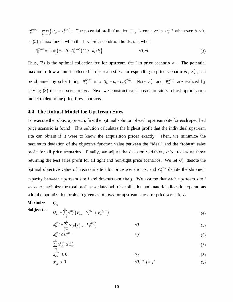
4.4 The Robust Model for Upstream Sites To execute the robust approach, first the optimal solution of each upstream site for each specified

price scenario is found. This solution calculates the highest profit that the individual upstream

site can obtain if it were to know the acquisition prices exactly. Then, we minimize the

maximum deviation of the objective function value between the “ideal” and the “robust” sales

profit for all price scenarios. Finally, we adjust the decision variables, 'sα , to ensure those

returning the best sales profit for all tight and non-tight price scenarios. We let *iOω denote the

optimal objective value of upstream site i for price scenario ω , and ( )TrijC denote the shipment

capacity between upstream site i and downstream site j. We assume that each upstream site i

seeks to maximize the total profit associated with its collection and material allocation operations

with the optimization problem given as follows for upstream site i for price scenario ω .

Maximize iOω

Subject to: ( )( ) ( ) ( )*

1

nTr Tr Co

i ij j ij ij

O x P V Pω ω ω ω=

= − +∑ (4)

( )( ) ( )' ' '

' 1

nTr Tr

ij ijj j ijj

x P Vω ωα=

= −∑ j∀ (5)

( ) ( )Tr Trij ijx Cω ≤ j∀ (6)

( ) *

1

nTr

ij ij

x Sω ω=

≤∑ (7)

( ) 0Trijx ω ≥ j∀ (8)

' 0ijjα > , ', 'j j j j∀ = (9)

11

' 0ijjα ≤ , ', '.j j j j∀ ≠ (10)

The objective function (4) is the sum of the sales profits and collection fees. Constraints (5)

are the material flow function definitions for emanating arcs from upstream site i. Constraints

(6) and (7) provide capacity limits for each arc and for the recycled item source. Constraints (8),

(9), and (10) are sign restrictions for unknown variables. Obviously, the material flow variables, ( )Trijx ω , are nonnegative, and the sign restrictions for 'sα require that the upstream site has more

incentive to ship more flow on the arc where its destination price offer is increased, but less

incentive when other downstream sites offer higher prices competing the material flow.

Next, we determine the robust flow function, or a common set of coefficients, 'sα , to be

evaluated in every price scenario ω∈Ω for site i. Thus, for each price scenario we subtract the

robust objective function value ( iRω ) using the common set of robust coefficients from the

optimal objective value ( *iOω ) of realization of acquisition price offers. The min-max robust

optimization model over all price scenarios for upstream site i can be stated as:

Minimize iδ Subject to: *

i i iO Rω ωδ ≥ − ω∀ (11)

( )( ) ( ) ( )*

1

nTr Tr Co

i ij j ij ij

R x P V Pω ω ω ω=

= − +∑ ω∀ (12)

( )( ) ( )' ' '

' 1

nTr Tr

ij ijj j ijj

x P Vω ωα=

= −∑ ,j ω∀ (13)

( ) ( )Tr Trij ijx Cω ≤ ,j ω∀ (14)

( ) *

1

nTr

ij ij

x Sω ω=

≤∑ ω∀ (15)

( ) 0Trijx ω ≥ ,j ω∀ (16)

' 0ijjα > , ', 'j j j j∀ = (17)

' 0ijjα ≤ , ', '.j j j j∀ ≠ (18)

The minimum maximum deviation *iδ of upstream site i is realized after solving the min-max

robust optimization model. The final step of the upstream model is solving the following model

to optimality to ensure that the decision variables, 'sα , return the best sales profit for non-

effective price scenarios (non-tight price scenarios in (11)) for upstream site i. The model for

each upstream site i is:

12

Maximize iRωω∈Ω∑

Subject to: * *i i iO Rω ωδ ≥ − ω∀

Constraints set of (12) - (18).

Given the robust solution values for α , the upstream site models determine robust flow

functions for each independent upstream site. Thus, the robust flow function describing the flow

shipment from upstream site i to downstream site j, denoted by ( )Trijx , is represented as

( )( ) ( )' ' '

'=1 ,

nTr Tr

ij ijj j ijj

x p V i jα= − ∀∑ (19)

where 'jp is the acquisition price offered by downstream site 'j . Note that the price scenario ω

is not an argument in the flow function at this point, and that (19) describes the material flow

relationship of the amount and acquisition price between upstream and downstream tiers. Each

upstream site provides each downstream site with a robust flow function to govern the material

flow transactions between them. The general form of the price-flow contract for each arc shown

in (19) represents not only the coordination between tiers but also the competition within the tier.

For example, in the price-flow contract of arc (i, j) associated with upstream site i, site i specifies

both how downstream site j’s acquisition price affects the flow on arc (i, j) and how other

downstream sites’ acquisition prices influence the flow on arc (i, j). If an upstream entity

determines its price-flow contract based on only the price of the specific downstream j it is

considering, the price-flow contract is found by setting the rest of the ' sα equal to zero in the

upstream model. In the next section, we present downstream site models to solve for the

equilibrium acquisition prices between these two tiers.

5. The Downstream Model: The Equilibrium Price Downstream sites are involved in transactions with upstream sites and customers in final demand

markets since they wish to obtain recycled items from upstream tier and sell the materials or sub-

components after refurbished/demanufacturing processes. Downstream sites make decisions on

their own acquisition prices subject to their constraints of processing capacities, transportation

capacities, and technology restrictions. We develop an equilibrium model of competitive

downstream sites to determine the Nash equilibrium price where no downstream site can

improve its objective function value by a unilateral change in its price solution. In this paper, we

13

utilize the relaxation algorithm (see Krawczyk and Uryasev 2000; Contreras et al. 2004) to find

the Nash equilibrium price solution.

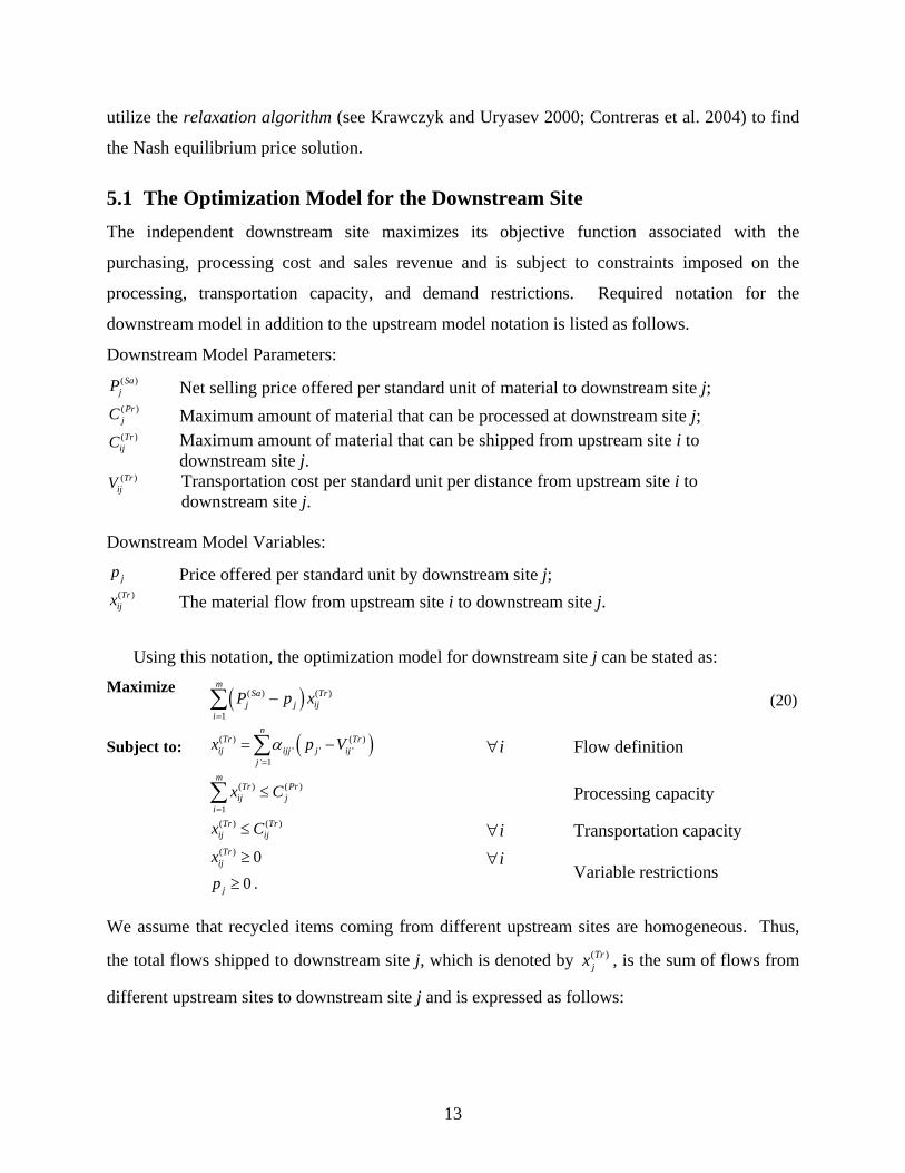
5.1 The Optimization Model for the Downstream Site The independent downstream site maximizes its objective function associated with the

purchasing, processing cost and sales revenue and is subject to constraints imposed on the

processing, transportation capacity, and demand restrictions. Required notation for the

downstream model in addition to the upstream model notation is listed as follows.

Downstream Model Parameters: ( )SajP Net selling price offered per standard unit of material to downstream site j; ( )PrjC Maximum amount of material that can be processed at downstream site j; ( )TrijC Maximum amount of material that can be shipped from upstream site i to

downstream site j. ( )Tr

ijV Transportation cost per standard unit per distance from upstream site i to downstream site j.

Downstream Model Variables:

jp Price offered per standard unit by downstream site j; ( )Trijx The material flow from upstream site i to downstream site j.

Using this notation, the optimization model for downstream site j can be stated as:

Maximize ( )( ) ( )

1

mSa Tr

j j iji

P p x=

−∑

(20)

Subject to: ( )( ) ( )' ' '

' 1

nTr Tr

ij ijj j ijj

x p Vα=

= −∑ i∀ Flow definition

( ) ( )

1

mTr Pr

ij ji

x C=

≤∑ Processing capacity

( ) ( )Tr Trij ijx C≤ i∀ Transportation capacity

( ) 0Trijx ≥ i∀

0jp ≥ . Variable restrictions

We assume that recycled items coming from different upstream sites are homogeneous. Thus,

the total flows shipped to downstream site j, which is denoted by ( )Trjx , is the sum of flows from

different upstream sites to downstream site j and is expressed as follows:

14

( )( ) ( ) ( )' ' '

1 1 '=1

= .m m n

Tr Tr Trj ij ijj j ij

i i j

x x p V jα= =

= − ∀∑ ∑∑ (21)

Here, the material flow variable for recycled items shipped to downstream site j, ( )Trjx , is the

function of acquisition prices of all downstream sites. Hence in order for the downstream site to

compute its optimal price bid, it must know the bids of the other downstream sites, and only this.

The optimization model of (20) for downstream site j can be generally transformed into the

model shown in (22), expressed in acquisition price variables where 1= ( , , )np pp L are the

collective price actions and where jφ is the payoff (or objective) function of downstream site j.

Let jdg denote the row d of constraint function and j

db the right-hand-side parameter of row d in

downstream site j’s optimization model.

Maximize ( )jφ p (22)Subject to:

1 1( )

( )

j j

j jr r

g b

g b

≤

≤

p

pM

0jp ≥

Next, we show the convex property of downstream site models for the existence and uniqueness

of the Nash equilibrium acquisition price solution.

Proposition 1 The optimization model for downstream site j, j = 1,…, n, has a strictly concave

objective function with respect to jp and a convex constraint set.

Proof. Trivially the set of linear constraints is a convex set with respect to price variables

(Nemhauser and Wolsey 1999).

Again, the format of the material flow variable ( )Trjx is written as ( )( )

' ' '1 ' 1

m nTr

ijj j iji j

p Vα= =

−∑∑ where

all coefficients 'sα are given by upstream sites and ( )TrijV are transportation cost parameters.

The only unknown variables are all 'p s . The variable ( )Trjx can be rewritten as:

( )1 1

Tr j jj n n jx p p Cα α= + + +L (23)

where jC is a constant and 'jjα is the coefficient term with 'jp for downstream site j’s model.

The interpretation of (23) is that the material flows shipped to downstream site j are a function of

price jp and also functions of other price variables offered by other downstream sites. Clearly,

the material flow is increasing as the price offer increases but decreasing when the competitors’

15

prices increase, if there exists a price effect between downstream site j and other downstream

sites. Thus, we have the following inequality relations

0jjα > and ' 0 ', 'j

j j j jα ≤ ∀ ≠ . (24)

From (24), the sign of second derivative of the objective function jφ can be determined as

2

2 0j

jpφ∂

<∂

.

Proposition 2 The impact of the change of acquisition price jp , j=1, 2,…,n, on the material

flow ( )Trjx is greater than the total impact on ( )Tr

jx due to the price changes from the rest of

downstream sites.

Proof. For every upstream site i, we have ' 0ijjα > for all , 'j j when j is equal to 'j , and ' 0ijjα ≤

for all , 'j j when j is not equal to 'j . In order to ensure a positive robust objective function for

each arc between the upstream and downstream tier in all of price scenarios, ω, we have

'' 1'

n

ijj ijjjj j

α α=≠

> ∑ for all i and j. Therefore, '' 1'

nj jj j

jj j

α α=≠

> ∑ for all j and it completes the proof.

In the next section, we provide some concepts and the required notation for the illustration of

the downstream site model algorithm.

5.2 Definitions and Concepts There are j = 1,…, n downstream sites participating in competing the material flows with the

price. Each downstream site j, j = 1,…, n, can adopt an individual price setting denoted by

j jp P∈ , where Pj is the set of price actions that downstream site j can choose. All downstream

entities, when acting together, can take a collective action, which is a vector 1= ( , , )np pp L .

Denote the collective price action set by P, and, by definition, 1 2 nP P P P⊆ × × ×L . Let

1= ( , , )np pp L and 1= ( , , )nq qq L be elements of the collective price action set 1 2 nP P P× × ×L .

The following notation and terminology are based upon (Krawczyk and Uryasev 2000;

Contrearas et al. 2004). An element 1 1 1( | ) ( , , , , , , )j j j j nq p p q p p− +≡p L L of the collective price

action set can be interpreted as a set of price actions where the jth downstream entity selects

16

price offer jq while the remaining entities are taking price jp , j = 1, 2,…, j-1, j+1,…, n. A

price action set * *1( , , )np p=*p L is called the Nash equilibrium price if, for downstream site j,

( | )( ) max ( | )

jj j j

ppφ φ

∈=

*

* *

pp p

P.

Note that at the Nash equilibrium solution, no entity can improve its individual objective

value by a unilateral change in its price decisions. In order to compute the Nash equilibrium, we

introduce the Nikaido-Isoda function (Nidaido and Isoda 1955). This function transforms an

equilibrium problem into an optimization problem (Contreras et al. 2004). The Nikaido-Isoda

function 1: ( )nP PΨ × × ×L 1( )nP P× × →ℜL is defined as:

1

( , )= ( | ) ( )n

j j jj

qφ φ=

⎡ ⎤Ψ −⎣ ⎦∑p q p p .

Each summand of the Nikaido-Isoda function can be viewed as the change in the objective

function value when its price action changes from pj to qj for all sites j in the downstream tier,

while all other downstream sites continue to choose according to price vector p. This means that

one entity changes its price action while others do not. Thus, the function represents the sum of

these changes in objective functions. Krawczyk and Uryasev (2000) claim that the function is

non-positive for all feasible q when p* is a Nash equilibrium solution, since no entity can

improve its objective function value at equilibrium by unilaterally alternating its solution. This

observation is used to construct a termination condition for the relaxation algorithm, such that

when an ε is chosen, the Nash equilibrium is obtained when max ( , )P

ε∈

Ψ <s

qp q , where s is the

iterative step of the relaxation algorithm.

Finally we introduce the optimum response function which returns the set of downstream

entities’ price actions whereby they all try to unilaterally maximize their respective objective

function values. The optimum response function (Krawczyk and Uryasev 2000) at the price

vector p is expressed in (25).

q( )=arg max ( , ) , ( )

PZ Z P

∈Ψ ∈p p q p p . (25)

Next, we illustrate the relaxation algorithm to solve for the Nash Equilibrium acquisition prices

between upstream and downstream tiers.

17

5.3 The Relaxation Algorithm The relaxation algorithms are used by (Krawczyk and Uryasev 2000; Contreras et al. 2004) for

different applications. We apply the relaxation algorithm to iteratively search for the Nash

equilibrium acquisition price solution of downstream site models. At each iteration of the

algorithm, downstream sites wish to move to a price point that represents an improvement on the

current price point. Having an initial estimate price vector, p0, the relaxation algorithm is shown

as follows:

1 (1 ) ( ) 0, 1, 2,s s ss sZ sβ β+ = − + =p p p L . (26)

where 0 1sβ< ≤ . The iterative step s+1 is constructed as a weighted average of the

improvement price point ( ) sZ p and the current price point sp . The optimum response function

( ) sZ p returns the next best move of price solutions by solving the quadratic convex model

shown in (20); in turn, each downstream site is trying to maximize its objective function by

unilaterally moving its price solution given others’ price solution. The iteration at each step is

constructed as a weighted average of the improvement solution ( ) Z p and the current price

solution p. By taking a sufficient number of iterations, the algorithm converges to the Nash

equilibrium price p* with a specified precision.

It is also interesting to note that the concept of the algorithm itself matches the idea of a

decentralized view on downstream sites. In each iteration, every entity can access all entities’

previous price actions and determines its best move in price decision based on its own interests

and constraints. In other words, the problem is a calculation of the succession of price decisions,

where entities choose their optimum response given the price decisions of the competitors in the

previous iteration.

The following theorem states the conditions of existence and uniqueness of the Nash

equilibrium solution and the convergence of the relaxation algorithm. Our optimization

downstream models satisfy these conditions, which is proven in Corollary 1. First we state

required definitions as follows (see Contreras and Krawczyk 2004). Let : P PΨ × →ℜ be a

function defined on a product P P× , where P is a convex closed subset of the Euclidean space nℜ . Further, we consider that ( , )Ψ p q is weakly convex-concave if it satisfies the following

inequalities.

18

( , ) (1 ) ( , ) ( (1 ) , ) (1 ) ( ,0 1(and 0, as 0, ,

r Pr P

β β β β β β βΨ + − Ψ ≥ Ψ − + − ∀ ∈ ≤ ≤

→ → ∀ ∈

z

z

x z y z x + y z x,y) x,y,zx,y) x - y z

x - y

and

( , ) (1 ) ( , ) ( (1 ) ) (1 ) ( ,0 1(and 0, as 0,

P

P

β β β β β β µ βµ

Ψ + − Ψ ≤ Ψ − + − ∀ ∈ ≤ ≤

→ → ∀ ∈

z

z

z x z y z, x + y x,y) x,y,zx,y) x - y z

x - y

where (rz x, y) and (µz x, y) are called the residual terms.

In other words, a function Ψ of two vector arguments is referred to as weakly convex-

concave if it satisfies weak convexity with respect to its first argument and weak concavity with

respect to its second argument. The notions of weak convexity and concavity are relaxations of

strict convexity and concavity (Berridge and Krawczyk 1997). The residual terms, to be chosen

at will, ensure that there are many concave functions which are weakly convex and many convex

functions which are weakly concave.

Theorem 1 (Uryasev and Rubinstein 1994) There exists a unique Nash equilibrium point to

which the relaxation algorithm converges if :

(1) P is a convex compact subset of nℜ ,

(2) the Nikaido-Isoda function : P PΨ × →ℜ is a weakly convex-concave function and ( , ) 0Ψ =p p

for P∈p ,

(3) the optimum response function ( ) Z p is single-valued and continuous on P,

(4) the residual term (rz x,y) is uniformly continuous on P with respect to z for all P∈x,y ,

(5) the residual terms satisfy

( ( r Pµ λ≥ ∈y xx,y) - y,x) ( x - y ) x, y where (0) 0λ = and λ is a strictly increasing function,

(6) the relaxation parameters sβ satisfy (a) 0sβ > , (b) 0

ss

β∞

=

= ∞∑ , and (c) 0 as s sβ → →∞ .

Corollary 1 There exists a unique Nash equilibrium price solution for downstream sites to

which the relaxation algorithm converges.

Proof. We need to verify that our downstream models satisfy the conditions (1) to (6) in

Theorem 1.

Condition (1): it is trivially satisfied.

19

Condition (2): from (23), we have that the material flows shipped to downstream site j, j =

1,…,n, is expressed as ( )1 1

Tr j jj n n jx p p Cα α= + + +L . After algebra manipulations, the objective

function of downstream site j is simply expressed in (27), where Vj is a constant parameter for

downstream site j.

1 1( ) ( )( )j jj j j n n jV p p p Cφ α α= − + + +p L . (27)

For any solution 1 1 1( | ) ( , , , , , , )j j j j nz p p z p p P− += ∈p L L and 1 1 1( | ) ( , , , , , , )j j j j nz q q z q q P− += ∈q L L ,

( | ) (1 ) ( | )j j j jz zβφ β φ+ −p q

1 1 1 1 1 1

1 1 1 1 1 1

( )( )

+(1- )( )( )

j j j j jj j j j j j j j n n j

j j j j jj j j j j j j j n n j

V z p p z p p C

V z q q z q q C

β α α α α α

β α α α α α− − + +

− − + +

= − + + + + + +

− + + + + + +

L L

L L

1 1 1 1 1 1

1 1 1

( )[ [ (1- ) ] [ (1- ) ]

[ (1- ) ] [ (1- ) ] ]

j j jj j j j j j j

j jj j j n n n j

V z p q p q z

p q p q C

α β β α β β α

α β β α β β− − −

+ + +

= − + + + + +

+ + + + +

L

L

( | (1- ) )j jzφ β β= p + q . Thus,

( | ) (1 ) ( | ) ( | (1- ) )j j j j j jz z zβφ β φ φ β β+ − =p q p + q j∀ . (28)

Since the objective functions jφ for all downstream sites are concave, we have

( ) (1 ) ( ) ( (1- ) )j j jβφ β φ φ β β+ − ≤p q p + q j∀ . (29)

Combining (28) and (29), the following inequality is satisfied. [ ( | ) ( )] (1 )[ ( | ) ( )] ( | (1- ) ) ( (1- ) )j j j j j j j j jz z zβ φ φ β φ φ φ β β φ β β− + − − ≥ −p p q q p + q p + q j∀ . (30)

Summing up all inequalities of (30) for all downstream site j, it implies that

1 1 1[ ( | ) ( )] (1 ) [ ( | ) ( )] [ ( | (1- ) ) ( (1- ) )]

n n n

j j j j j j j j jj j j

z z zβ φ φ β φ φ φ β β φ β β= = =

− + − − ≥ −∑ ∑ ∑p p q q p + q p + q . (31)

The definition of the Nikaido-Isoda function is referred to (31), we have

( , (1- ) ( , ( (1- ) ,β β β βΨ Ψ ≥ Ψp z) + q z) p + q z) . (32)

From (32), the Nikaido-Isoda function Ψ is convex with respect to the first argument. Based on

the same algebra manipulation, the function Ψ is also concave with respect to the second

argument which is

( , (1- ) ( , ( (1- )β β β βΨ Ψ ≤ Ψz p) + z q) z, p + q) . (33)

From (32) and (33), the Nikaido-Isoda function Ψ is convex-concave which is also weakly

convex-concave. Then, the optimization model for each downstream site j satisfies Condition

(2).

20

Condition (3): the optimum response function ( ) Z p is single-valued and continuous on P by

solving the concave quadratic convex constrained model.

Condition (4): if the Nikaido-Isoda function ( ,Ψ p q) is twice continuously differentiable with

respect to both arguments on the set P P× , the residual term is given by (Uryasev and

Rubinstein 1994)

21( ( )( ), ( )2

r A o+z p,q) = p,p p - q p - q p - q

where ,• • is the notation of inner product and ( ) ( , |pp q pA == Ψp,p p q) is the Hessian of the

Nikaido-Isoda function with respect to the first argument evaluated at q = p. Moreover, if the

function ( ,Ψ p q) is convex with respect to p, then 2( ) 0o =p - q (Uryasev 1988). The residual

term of (rz p,q) is a polynomial expression which is continuous on P. Furthermore, (rz p,q) is

uniformly continuous on P since P is compact (Bartle 1976).

Condition (5): assuming that ( ,Ψ p q) is twice continuously differentiable, in order to prove

this condition, it suffices to show that ( , | ( , |pp q p qq q p= =Ψ −Ψp q) p q) is positive definite (Krawczyk

and Uryasev 2000), where ( , |pp q p=Ψ p q) is the Hessian of the Nikaido-Isoda function with respect

to the first argument and ( , |qq q p=Ψ p q) is the Hessian of the Nikaido-Isoda function with respect

to the second argument, both evaluated at q = p.

The Hessian matrices of the Nikaido-Isoda function are shown in (34) and (35) respectively.

( , |pp q p=Ψ =p q)

1 1 2 11 2 1 1

2 1 21 2 2

11

22

2

nn

n nn n

α α α α αα α α

α α α

⎛ ⎞+ +⎜ ⎟

+⎜ ⎟⎜ ⎟⎜ ⎟⎜ ⎟+⎝ ⎠

L

M

M O

L

. (34)

( , |qq q p=Ψ =p q)

11

22

2 0 00 2

0 2 nn

αα

α

⎛ ⎞−⎜ ⎟

−⎜ ⎟⎜ ⎟⎜ ⎟⎜ ⎟−⎝ ⎠

L

M

M O

L

. (35)

( , | ( , |pp q p qq q p= =Ψ −Ψ =p q) p q)

1 1 2 11 2 1 1

2 1 21 2 2

11

44

4

nn

n nn n

α α α α αα α α

α α α

⎛ ⎞+ +⎜ ⎟

+⎜ ⎟⎜ ⎟⎜ ⎟⎜ ⎟+⎝ ⎠

L

M

M O

L

.

21

As discussed in Proposition 1, we require that 0jjα > and ' 0 ', 'j

j j j jα ≤ ∀ ≠ . Since all pivots

for the matrix of ( , | ( , |pp q p qq q p= =Ψ −Ψp q) p q) are positive, ( , |pp q p=Ψ p q) ( , |qq q p=−Ψ p q) is positive

definite (Strang 1986). We can conclude that the optimization models of downstream sites

satisfy Condition (5).

Condition (6): in order for the algorithm to converge, we may choose any sequence ( sβ )

satisfying the Condition (6) of Theorem 1.

All conditions in Theorem 1 are satisfied for the optimization model of downstream sites. It

completes the proof.

The Relaxation Algorithm states that each downstream site is trying to maximize its

objective function by unilaterally moving its price solution given others’ previous price

solutions. The algorithm itself essentially is in an iterative scheme and continues until all of

downstream sites find the Nash equilibrium acquisition price solution where no downstream site

is willing to alter its acquisition price based on the price-flow contracts given by associated

upstream sites. In the next section, we summarize the solution algorithm consisting of upstream

and downstream models and explicitly illustrate the decision-making procedures under this

framework of Section 4 and 5.

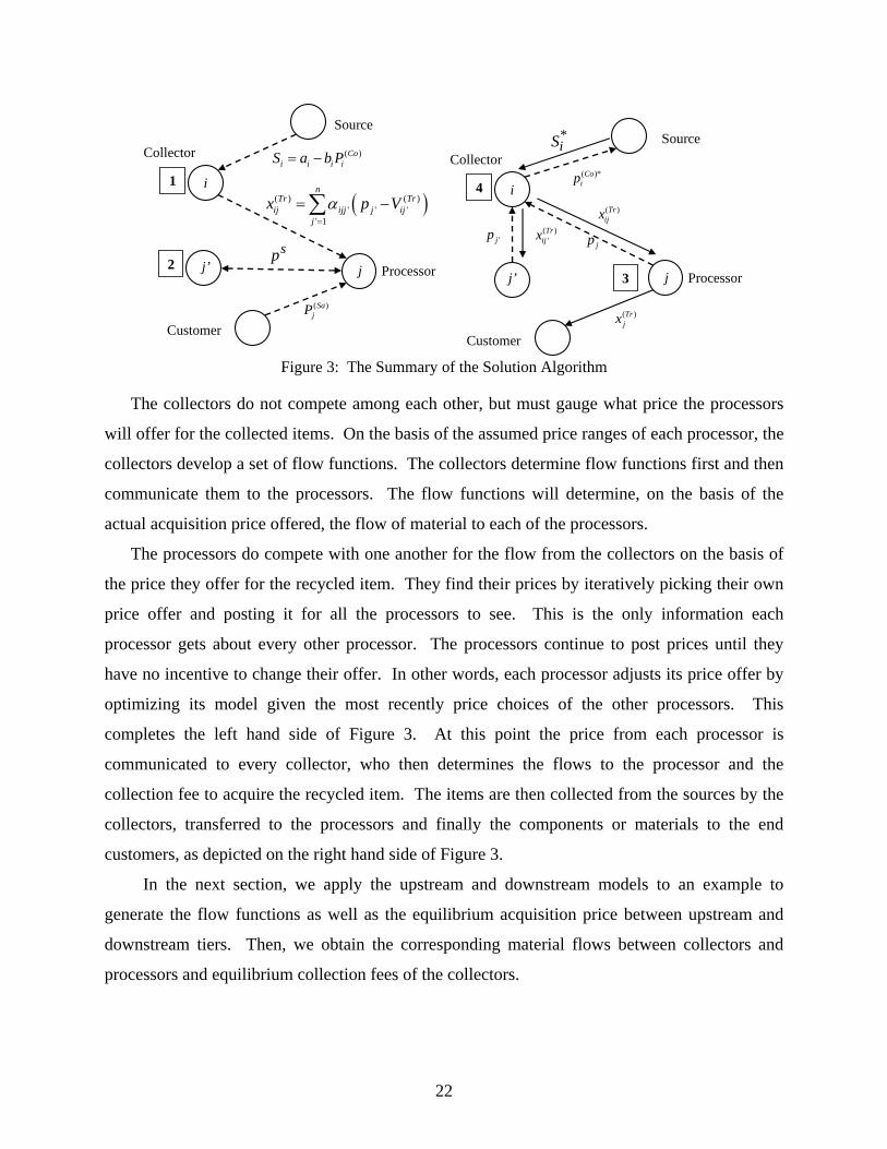
6. The Summary of the Solution Algorithm The overall reverse production system is comprised of four entities: sources, collectors,

processors and customers as shown in Figure 3. The material flows are represented as solid

lines, information communication is denoted by the dashed line, and the steps of the solution

algorithm are illustrated by the number in the rectangle box in Figure 3. The behavior of the

source and the customer is assumed simple. The source supplies the collector on the basis of a

fee charged by the collector, and the relationship is known by both parties. We assume that this

is linear in the fee, with a decreasing flow for a higher collection fee. The source can be thought

of as the aggregate behavior of many independent entities that have a given product ready for

disposal that will choose to go, or not to go, to a collector based on the fee. The customers have

a fixed price for a given material or sub-component and the market is assumed to be very large

such that the flow from processors to customers does not change the price. The customers

communicate the price to the processors at the outset, but it is not considered private

information.

22

i

Source

Customer

( )Coi i i iS a b P= −

( )( ) ( )' ' '

' 1

nTr Tr

ij ijj j ijj

x p Vα=

= −∑

)(SajP

1

jsp2

i

Source

Processor

Customer

4

j3j’

'jpjp

( )*Coip

( )Trjx

( )Trijx

( )'Tr

ijx

*iS

j’

Collector Collector

Processor

Figure 3: The Summary of the Solution Algorithm

The collectors do not compete among each other, but must gauge what price the processors

will offer for the collected items. On the basis of the assumed price ranges of each processor, the

collectors develop a set of flow functions. The collectors determine flow functions first and then

communicate them to the processors. The flow functions will determine, on the basis of the

actual acquisition price offered, the flow of material to each of the processors.

The processors do compete with one another for the flow from the collectors on the basis of

the price they offer for the recycled item. They find their prices by iteratively picking their own

price offer and posting it for all the processors to see. This is the only information each

processor gets about every other processor. The processors continue to post prices until they

have no incentive to change their offer. In other words, each processor adjusts its price offer by

optimizing its model given the most recently price choices of the other processors. This

completes the left hand side of Figure 3. At this point the price from each processor is

communicated to every collector, who then determines the flows to the processor and the

collection fee to acquire the recycled item. The items are then collected from the sources by the

collectors, transferred to the processors and finally the components or materials to the end

customers, as depicted on the right hand side of Figure 3.

In the next section, we apply the upstream and downstream models to an example to

generate the flow functions as well as the equilibrium acquisition price between upstream and

downstream tiers. Then, we obtain the corresponding material flows between collectors and

processors and equilibrium collection fees of the collectors.

23

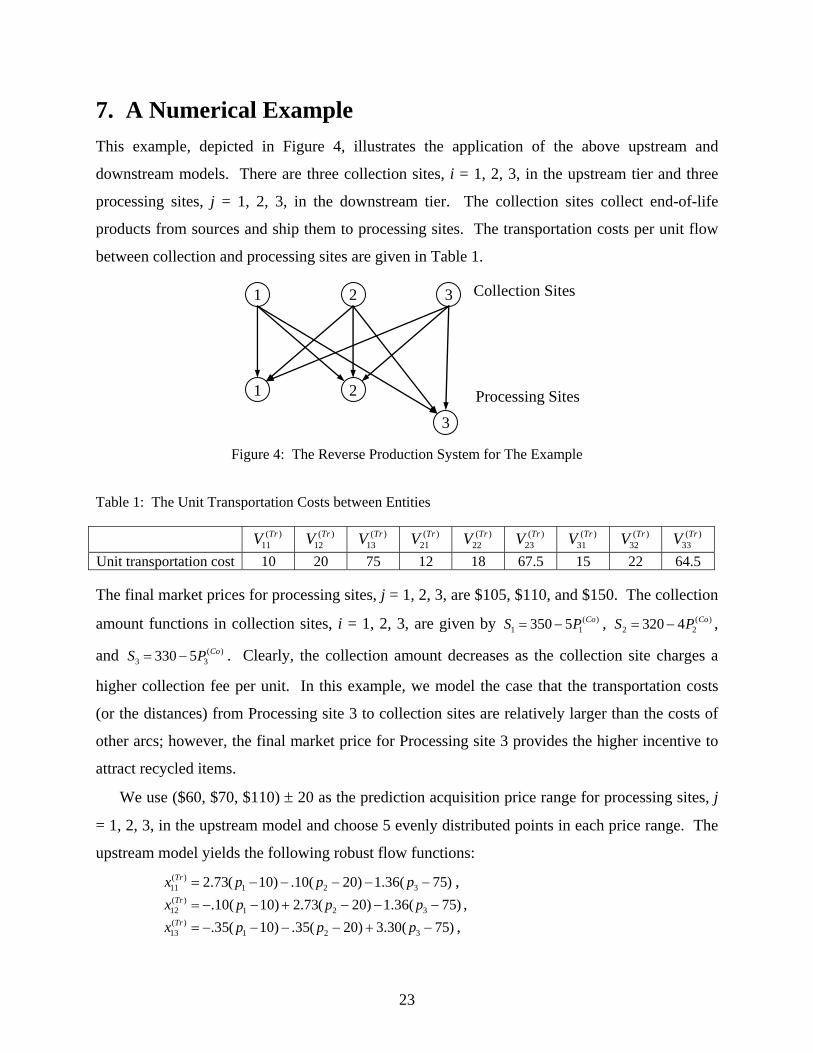
7. A Numerical Example This example, depicted in Figure 4, illustrates the application of the above upstream and

downstream models. There are three collection sites, i = 1, 2, 3, in the upstream tier and three

processing sites, j = 1, 2, 3, in the downstream tier. The collection sites collect end-of-life

products from sources and ship them to processing sites. The transportation costs per unit flow

between collection and processing sites are given in Table 1.

Processing Sites

1

1

2

2

3

3

Collection Sites

Figure 4: The Reverse Production System for The Example

Table 1: The Unit Transportation Costs between Entities

( )11

TrV ( )12

TrV ( )13

TrV ( )21

TrV ( )22

TrV ( )23

TrV ( )31

TrV ( )32

TrV ( )33

TrV

Unit transportation cost 10 20 75 12 18 67.5 15 22 64.5 The final market prices for processing sites, j = 1, 2, 3, are $105, $110, and $150. The collection

amount functions in collection sites, i = 1, 2, 3, are given by ( )1 1350 5 CoS P= − , ( )

2 2320 4 CoS P= − ,

and ( )3 3330 5 CoS P= − . Clearly, the collection amount decreases as the collection site charges a

higher collection fee per unit. In this example, we model the case that the transportation costs

(or the distances) from Processing site 3 to collection sites are relatively larger than the costs of

other arcs; however, the final market price for Processing site 3 provides the higher incentive to

attract recycled items.

We use ($60, $70, $110) ± 20 as the prediction acquisition price range for processing sites, j

= 1, 2, 3, in the upstream model and choose 5 evenly distributed points in each price range. The

upstream model yields the following robust flow functions:

( )11 1 2 32.73( 10) .10( 20) 1.36( 75)Trx p p p= − − − − − ,

( )12 1 2 3.10( 10) 2.73( 20) 1.36( 75)Trx p p p= − − + − − − ,

( )13 1 2 3.35( 10) .35( 20) 3.30( 75)Trx p p p= − − − − + − ,

24

( )21 1 32.72( 12) 1.22( 67.5)Trx p p= − − − ,

( )22 1 2 3.64( 12) 2.23( 18) .44( 67.5)Trx p p p= − − + − − − ,

( )23 1 3.88( 12) 2.65( 67.5)Trx p p= − − + − ,

( )31 1 2 32.78( 15) .73( 22) .31( 64.5)Trx p p p= − − − − − ,

( )32 1 2 3.08( 15) 2.67( 22) 1.06( 64.5)Trx p p p= − − + − − − ,

( )33 1 31.14( 15) 2.92( 64.5)Trx p p= − − + − .

We apply the relaxation algorithm to obtain the Nash Equilibrium acquisition prices

determined by processing sites. The detailed steps of the relaxation algorithm are illustrated in

Table 2. At iteration 7, the max ( ,P∈Ψ s

qp q) approaches to zero which indicates 7

1p , 72p , and 7

3p are

the Nash Equilibrium acquisition prices for processing sites 1, 2, and 3.

Table 2: The Calculation of the Relaxation Algorithm for the Example

Iteration(s) 1sp 2

sp 3sp 1( )sZ p 2( )sZ p 3( )sZ p sα 1

1sp + 1

2sp + 1

3sp +

1 60.00 60.00 60.00 58.73 65.79 116.72 1.00 58.73 65.79 116.72 2 58.73 65.79 116.72 68.95 76.36 116.67 0.99 68.85 76.25 116.67 3 68.85 76.25 116.67 69.47 76.90 118.23 0.98 69.46 76.88 118.20 4 69.46 76.88 118.20 69.77 77.22 118.33 0.97 69.76 77.21 118.32 5 69.76 77.21 118.32 69.81 77.26 118.37 0.96 69.81 77.25 118.37 6 69.81 77.25 118.37 69.82 77.27 118.38 0.95 69.82 77.27 118.38 7 69.82 77.27 118.38 69.82 77.27 118.38 0.94 69.82 77.27 118.38

The corresponding material flows between collection and processing sites and equilibrium

collection fees of collection sites are listed in Table 3 and Table 4 respectively.

Table 3: The Resulting Material Flows between Collection and Processing Sites

( )11

Trx ( )12

Trx ( )13

Trx ( )21Trx ( )

22Trx ( )

23Trx ( )

31Trx ( )

32Trx ( )

33Trx

Material flow 98.3 91.1 101.8 95.2 72.6 84.1 95.8 86.2 94.4 Table 4: The Equilibrium Collection Fees

( )*1

CoP ( )*2

CoP ( )*3

CoP Equilibrium collection fee 11.76 17.02 10.72

The preceding example demonstrates a two-tier and single-commodity decentralized RPS

problem that can be solved using the models given in Section 4 and 5. First, the upstream model

for each collection site provides the flow functions used to contract with processing sites. Then,

we solve for the Nash equilibrium acquisition prices between collection and processing sites by

the relaxation algorithm. Finally, we obtain the corresponding material flows between these two

tiers and the equilibrium collection fees of collection sites.

25

8. Conclusions and Extensions This paper presents a decentralized perspective for reverse production systems where each

independent entity considers its own objective function and is subject to its own constraints.

Meanwhile, the objective function of each entity not only depends on its own decision variables

but also depends on decision variables of other entities. In this paper, we focus on a two-tier

reverse production system involving the price and material flow decisions where the price-flow

contract is determined by upstream entities and the acquisition prices of material flows

transacted between upstream and downstream sites are determined by downstream entities. We

apply the min-max robust optimization on each of the independent upstream models to generate

the flow functions which are used to contract with downstream sites.

Downstream entities compete for material flows from the upstream tier. The iterated

relaxation algorithm is used to solve for the Nash equilibrium acquisition prices between

upstream and downstream sites. Note that the algorithm itself matches the idea of a

decentralized decision-making process where every downstream entity can access all entities’

previous price actions and determines its next best move for its price decision. We also show the

existence and uniqueness of the Nash Equilibrium price under reasonable assumptions about the

underlying functions of each entity. Then, the equilibrium acquisition prices from downstream

entities are communicated to associated upstream entities, who then determine the flows to the

downstream entities and the collection fees to acquire recycled items.

In this paper, upstream entities determine price-flow contracts by using a robust optimization

approach, but there are other criteria, such as an expected value and a max-min objective, that

may be used by different upstream entities. Also, many reverse production systems have

network structures that involve more than the two types of entities we have discussed here, and

with more than one type of item to be picked up and recycled. For example, computers, printers,

monitors and other auxiliary equipment are available from sources and may be converted into

commodities such as steel and copper through a supply chain that involves multiple processors

engaged in size reduction and smelting. The extension of our approach to these multi-tier

problems with multiple item types requires further refinement of the models we have developed.

Finally, the reverse supply chains differ general forward chains in that, in the former, the

government may involve more with policy making or evaluation. The model presented in this

paper is a prototype decentralized RPS model and can be used as a tool to analyze the issues of

26

the government-subsidy, price fluctuation, comparison of centralized vs. decentralized systems,

and other situations where the individual behavior of the supply chain components might be an

important overall factor in the system behavior.

Acknowledgments This research has been partially supported by the National Science Foundation under grants

DMI#0200162 and SBE-0123532 The authors are grateful for the generous interaction and

guidance provided from many industry experts, including Julian Powell of Zentech, Carolyn

Phillips and the staff of Reboot, Nader Nejad of Molam, Ken Clark of MARC5R, and Bob

Donaghue and Chuck Boelkins of P2AD. We appreciate the efforts and expertise of the previous

anonymous reviewers and are thankful for his/her careful comments and thoughtful reading of

the paper. We have found them greatly valuable to improving the current manuscript.

References Ammons, J. C., M. J. Realff, D. J. Newton. 2001. Decision models for reverse production

system design. Handbook of Environmentally Conscious Manufacturing. Kluwer Academic

Publishers, Boston, MA, 341-362.

Assavapokee, T., J. C. Ammons, M. Realff. 2005. A new min-max regret robust optimization

approach for interval data uncertainty. Submitted to Journal of Global Optimization.

Barros, A. I., R. Dekker, V. Scholten. 1998. A two-level network for recycling sand: a case

study. European Journal of Operational Research 110 199-214.

Berridge, S., J. B. Krawczyk. 1997. Relaxation algorithms in finding Nash equilibria.

Economic Working Paper, Institute of Statistics and Operations Research, Victoria

University of Wellington, New Zealand.

Bartle, R. G. 1976. The Elements of Real Analysis, 2nd edition. John Wiley & Sons, Inc.

Bazaraa, M. S., M. D. Sherali, C. M. Shetty. 1993. Nonlinear Programming, Theory and

Algorithms, 2nd edition. John Wiley & Sons, Inc.

Cachon, G. P., M. A. Lariviere. 2001. Contracting to assure supply: How to share demand

forecasts in a supply chain. Management Science 47(5) 629-646

27

Contreras, J., M. Klusch, J. B. Krawczyk. 2004. Numerical solutions to Nash-Cournot equlibria

in coupled constraint electricity markets. IEEE Transactions on Power Systems 19(1) 195-

206.

Corbett, C. J., U. S. Karmarkar. 2001. Competition and structure in serial supply chains with

deterministic demand. Management Science 47(7) 966-978.

Corbett, C. J., D. Zhou, C. S. Tang. 2004. Designing supply contracts: Contract type and

information asymmetry. Management Science 50(4) 550-559.

Donohue, K. L. 2000. Efficient supply contracts for fashion goods with forecast updating and

two production modes. Management Science 46(11) 1397-1411.

Flapper, S. D. P. 1995. On the operational aspects of reuse. Proceedings of the 2nd

International Symposium on Logistics, Nottingham, UK. 109-118.

Flapper, D. D. P. 1996. Logistic aspects of reuse: an overview. Proceedings of the 1st

International Working Seminar on Reuse, Eindhoven, The Netherlands. 109-118.

Fleischmann, M., H. R. Krikke, R. Dekker, S. D. P. Flapper. 2000. A characterization of

logistics networks for product recovery. Omega 28 653-666.

Fudenberg, D., J. Tirole. 1991. Game Theory. MIT Press, Cambridge, MA.

Guide, V. D. R., T. P. Harrison. 2003. The challenge of closed-loop supply chains. Interfaces

33(6) 3-6.

Guide, V. D. R., R. H. Teunter, L. N. Van Wassenhove. 2003. Matching demand and supply to

maximize profits from remanufacturing. Manufacturing & Service Operations Management

5(4) 303-316.

Hobbs, B. F. 2001. Linear complementarity models of Nash-Cournot competition in bilateral

and POOLCO power market. IEEE Transactions on Power Systems 16(2) 194-202.

Hong, I-H., T. Assavapokee, J. C. Ammons, C. Boelkins, K. Gilliam, D. Oudit, M. J. Realff, J.

M. Vannicola, W. Wongthatsanekorn. 2006. Planning the e-scrap reverse production system

under uncertainty in the state of Georgia: a case study. To appear in IEEE Transactions on

Electronics Packaging Manufacturing.

28

Huttunen, A. 1996. The Finnish solution for controlling the recovered paper flows.

Proceedings of the 1st International Seminar on Reuse. Eindhoven, The Netherlands. 177-

187.

Jayaraman, V., V. D. R. Guide, R. Srivastava. 1997. A closed-loop technical report, logistics

model for use within a recoverable manufacturing environment. Air Force Institute of

Technology, Wright-Patterson, OH.

Kouvelis, P., G. Yu. 1997. Robust Discrete Optimization and Its Applications. Kluwer, Boston,

MA.

Krawczyk, J. B., S. Uryasev. 2000. Relaxation algorithms to find Nash equlibria with economic

applications. Environmental Modeling and Assessment 5 63-73.

Krikke, H. R. 1998. Recovery strategies and reverse logistic network design. Ph.D.

dissertation, University of Twente, Enchede, The Netherlands.

Kroon, L., G. Vrijens. 1995. Returnable containers: an example of reverse logistics.

International Journal of Physical Distribution & Logistics Management 25(2) 56-68.

Lemke, C. E. 1965. Bimatrix equilibrium points and mathematical programming. Management

Science 11 681-689.

Majumder, P., H. Groenevelt. 2001. Competition in remanufacturing. Production and

Operations Management 10(2) 125-141.

Nagurney, A., F. Toyasaki. 2005. Reverse supply chain management and electronic waste

recycling: a multitiered network equilibrium framework for e-cycling. Transportation

Research Part E 41 1-28.

Nemhauser, G. L., L. A. Wolsey. 1999. Integer and Combinatorial Optimization. John Wiley

& Sons, Inc., New York, NJ.

Nicholson, W. 2002. Microeconomic Theory – Basic Principles And Extensions. Thomson

Learning, Inc.

Nikaido, H., K. Isoda. 1955. Note on noncooperative convex games. Pacific Journal of

Mathematics 5 807-815.

Pohlen, T. L., M. Farris II. 1992. Reverse logistics in plastic recycling. International Journal of

Physical Distribution & Logistics Management 22(7) 35-47.

29

Realff, M. J., J. C. Ammons, D. J. Newton. 2004. Robust reverse production system design for

carpet recycling. IIE Transactions 36 767-776.

Savaskan, R. C., S. Bhattacharya, L. N. Van Wassenhove. 2004. Closed-loop supply chain

models with product remanufacturing. Management Science 50(2) 239-252.

Savaskan, R. C., L. N. Van Wassenhove. 2006. Reverse channel design: The case of competing

retailers. Management Science 52(1) 1-14.

Shih, L.-H. 2001. Reverse logistics system planning for recycling electrical appliances and

computers in Taiwan. Resources, Conservation, and Recycling 32 55-72.

Strang, G. 1986. Linear Algebra and Its Applications. Harcourt Brace Jovanovich, Inc.

Thierry, M., M. Salomon, J. Van Nunen, L. Van Wassenhove. 1995. Strategic issues in product

recovery management. California Management Review 37(2) 114-135.

Thierry, M. 1997. An analysis of the impact of product recovery management on manufacturing

companies. Ph.D. dissertation, Erasmus University, Rotterdam, The Netherlands.

Tsay, A. A. 1999. The quantity flexibility contract and supplier-customer incentives.

Management Science 45(10) 1339-1358.

Uryasev, S., R. Y. Rubinstein 1994. On relaxation algorithms in computation of noncooperative

equilibria. IEEE Transactions on Automatic Control 39(6) 1263-1267.

Wang, H., M. Guo, J. Efstathiou. 2004. A geme-theoretical cooperative mechanism design for a

two-echelon decentralized supply chain. European Journal of Operational Research 157(2)

372-388.

Wang, C.-H., J. C. Even Jr., S. K. Adams. 1995. A mixed-integer linear model for optimal

processing and transport of secondary materials. Resources, Conservation, and Recycling 15

65-78.

Winston, W. L. 1994. Operations Research – Applications and Algorithms. Wadsworth, Inc.

Belmont, CA.