Embed Size (px)
Citation preview

December 4, 2000 © 2000 Fernando L. Alvarado 1
Reliability concepts and market power
Fernando L. AlvaradoProfessor, The University of Wisconsin
Invited Seminar at the U. S. Department of EnergyDecember 4, 2000

December 4, 2000 © 2000 Fernando L. Alvarado 2
Outline
• Reliability basics overview
• Some market power issues

December 4, 2000 © 2000 Fernando L. Alvarado 3
Basics overview (assumptions)
• Exactly two technologies– Each technology has a known price
• No market power
• Inelastic demand
• Reliability event occurs when demand exceeds supply

December 4, 2000 © 2000 Fernando L. Alvarado 4
Quantity (power)
Pri
ce
Dem
and
(ine
last
ic)
Available supply
Clearingprice
Maximumavailable
power
Deterministic Demand and Supply, low demand case

December 4, 2000 © 2000 Fernando L. Alvarado 5
Quantity (power)
Pri
ce
Dem
and
(ine
last
ic)
Available supply
Clearingprice
Maximumavailable
power
Deterministic Demand and Supply, high demand case

December 4, 2000 © 2000 Fernando L. Alvarado 6
Probabilistic Demand, high demand case
Outageprobability
Probability of low prices

December 4, 2000 © 2000 Fernando L. Alvarado 7
The piece-wise nature of the supply curve
Gen
erat
or 1
Gen
erat
or 2
Gen
erat
or 3
Gen
erat
or 4 G
ener
ator
5
Gen
erat
or 6

December 4, 2000 © 2000 Fernando L. Alvarado 8
The effect of a generator outage
Outagedgenerator
Oldsupply
limit
Newsupplylimit

December 4, 2000 © 2000 Fernando L. Alvarado 9
Effect of demand uncertainty and generator outage
n-1 secure
insecure
Probabilityp2
Outage probability is p1*p2
Probability p1

December 4, 2000 © 2000 Fernando L. Alvarado 10
System B
System A
Gen
erat
or 1
A
Gen
erat
or 2
A
Gen
erat
or 3
A
Gen
erat
or 4
A
Gen
erat
or 5
A
Gen
erat
or 6
A
Gen
erat
or 1
B
Gen
erat
or 2
B
Gen
erat
or 3
B
Gen
erat
or 4
B
Gen
erat
or 5
B
High pricen-1 insecureLow price
Secure

December 4, 2000 © 2000 Fernando L. Alvarado 11
System B
System AHigh pricen-1 secureLow price
n-1 secure

December 4, 2000 © 2000 Fernando L. Alvarado 12
System B
System ALow pricen-1 secureLow price
n-1 secure
Flow

December 4, 2000 © 2000 Fernando L. Alvarado 13
Temptation: construct a composite supply curve
+
Low pricen-1 secure
unnecessary

December 4, 2000 © 2000 Fernando L. Alvarado 14
Flow
Normal conditions
System B
System ALow pricen-1 insecureLow price
n-1 secure
Situation with line transmission limits
Maxflow
Maxflow
Outagedgenerator
Unableto clear

December 4, 2000 © 2000 Fernando L. Alvarado 15
System B
System AFlow
Maxflow
Use of distributed reserves
Low pricen-1 secureLow price
n-1 secure

December 4, 2000 © 2000 Fernando L. Alvarado 16
Features of the example
• Only two areas (one flowgate)
• Radial
• Demand is inelastic
• Time delays are not an issue
• Generators have no startup/shutdown costs or restrictions or minimum power levels

December 4, 2000 © 2000 Fernando L. Alvarado 17
Observations
• Demand elasticity is important• Locational aspects of reserves matter
– LMP for reserves
• Ramping rates matter• In deregulated markets only units explicitly
committed to reserves are available– In regulated markets and in PJM all units are
• Reliability requires that we increase supply– Standby charges tend to reduce supply (Tim Mount)

December 4, 2000 © 2000 Fernando L. Alvarado 18
Reality
• Many flowgates• Networked sysyem• Demand can be elastic• Time delays important• Generators have fixed
costs and restrictions• Load is uncertain
• Transmission outages exacerbate problems
• If one firm dominates a technology, market power occurs (next)
• If one firm dominates a location, market power results

December 4, 2000 © 2000 Fernando L. Alvarado 19
Market Power?
• The ability to raise prices significantly above the efficient economic equilibrium
• Disclaimer: the slides that follow are not really a market power study but rather they represent a simplified illustration of how higher prices could result as a result of market concentration.

December 4, 2000 © 2000 Fernando L. Alvarado 20
Market Power: Assumptions
• There are exactly two technologies– Each technology has a fixed marginal price availability of the expensive technology– Limited availability of the cheap technology– Cheap technology has fixed costs to recover
• Demand is inelastic– First deterministic, then probabilistic
• All suppliers but a schedule all their cheap power• Supplier a owns P MW in n1 equal-sized generators
– Supplier a can “withhold” one or more generators– Bidding above marginal cost is not allowed, withholding isBidding above marginal cost is not allowed, withholding is

December 4, 2000 © 2000 Fernando L. Alvarado 21
The piece-wise nature of the supply curve revisited
Oth
er s
uppl
iers
Sup
plie
r a
gene
rato
r 1
Dem
and
Clearingprice
If generators bid marginal price,the generators surplus is zero
Sup
plie
r a
gene
rato
r 2

December 4, 2000 © 2000 Fernando L. Alvarado 22
Red generator decides to withhold one generator
Withheldgenerator
Clearingprice
Sur
plus
for
red
supp
lier
Red supplier nowhas large surplus
Of course blue supplierhas even LARGER surplus!
Sur
plus
for
blue
sup
plie
r

December 4, 2000 © 2000 Fernando L. Alvarado 23
If margins are increased
Clearingprice
Now it is not possible for redsupplier to withhold and gain
Raising priceswould requirecollusion
Question: and how are theexpensive technology units
supposed to recover theirfixed costs if they always
clear at their marginal cost?
Answer: you may endup with less capacitythan you thought

December 4, 2000 © 2000 Fernando L. Alvarado 24
If demand is uncertain
The expected surplusgain is: p*(2-1)*P1
Probability p thatwithholding willresult in surplus
2
P1
price 1
Quantity (power)
Pri
ce
Since 1 is cheap unit’s marginalcost, there is no expected surplus loss

December 4, 2000 © 2000 Fernando L. Alvarado 25
Additional observations
• If the margin to the “knee” is Pm, any supplier with a total ownership above Pm may profit from withholding– If more than one supplier meets this conditions,
chances are that someone will withhold

December 4, 2000 © 2000 Fernando L. Alvarado 26
For two generators, surplusis P*(2-1)/2 for demandabove this level
Effect of “granularity”
With only onegenerator, it isimpossible towithhold andbenefit P
Surplus is P*(2-1) fordemand above this level

December 4, 2000 © 2000 Fernando L. Alvarado 27
Effect of “granularity,” three generator case
Surplus is P*(2-1)/3 fordemand above this level
Surplus is 2P*(2-1)/3 fordemand above this level

December 4, 2000 © 2000 Fernando L. Alvarado 28
Effect of “granularity”
Sur
plus
With n=1, there is no surplus
Surplus with n=2
Surplus with n=3
Surplus with n=4
Surplus with n
Demand level

December 4, 2000 © 2000 Fernando L. Alvarado 29
Observations and assumptions
• For “worst case” effect, assume n=• Assume withholding will occur
– Withholding “softens” the supply curve
• High cost periods needed for fixed cost recovery• Demand is probabilistic• Suggestion: market power occurs if expected
surplus exceeds fixed cost recovery– This is also a signal for system expansion
• This means that in the absence of uncertainty, expansion will occur when expected profits exceed long run marginal costs

December 4, 2000 © 2000 Fernando L. Alvarado 30
Effect of number of suppliers on supply curve
One supplier
2 su
pplie
rs3
supp
liers
10 s
uppl
iers
Demand
Pri
ce

December 4, 2000 © 2000 Fernando L. Alvarado 31
Pri
ce
Demand
Period during whichfixed cost recoverycan take place
Effect of demand uncertainty on fixed cost recovery
Withholding increases the period duringwhich surplus accrues but reduces theamount that accrues

December 4, 2000 © 2000 Fernando L. Alvarado 32
Pri
ce
Demand
Period during whichfixed cost recoverycan take place
The effect of demand uncertainty on fixed cost recovery
December 4, 2000 © 2000 Fernando L. Alvarado 33
Numerical studies
• Demand is 60/70/80/90/95% of “knee”
• for demand varies from 0 to 20%
• Demand probability distribution is normal
• Supplier has equal size units available
• There are 3/6/10/15/ suppliers
We illustrate the fixed costs that can be recoveredfor each of the case combinations above accordingto our earlier withholding assumptions

December 4, 2000 © 2000 Fernando L. Alvarado 34
0 0.02 0.04 0.06 0.08 0.1 0.12 0.14 0.16 0.18 0.20
50
100
150
200
250
80%
Variance of demand (per unit)
Fixed cost recovery without market power ( suppliers)
Tho
usan
ds p
er y
ear
per
MW
90%
95%
99% Demand level as a percentageof available capacity
December 4, 2000 © 2000 Fernando L. Alvarado 35
0 2 4 6 8 10 12 14 16 18 200
20
40
60
80
100
120
140
160
180
200
Demand Variance (percent)
Fix
ed
co
st r
eco
very
(th
ou
san
ds
per
MW
-yea
r)
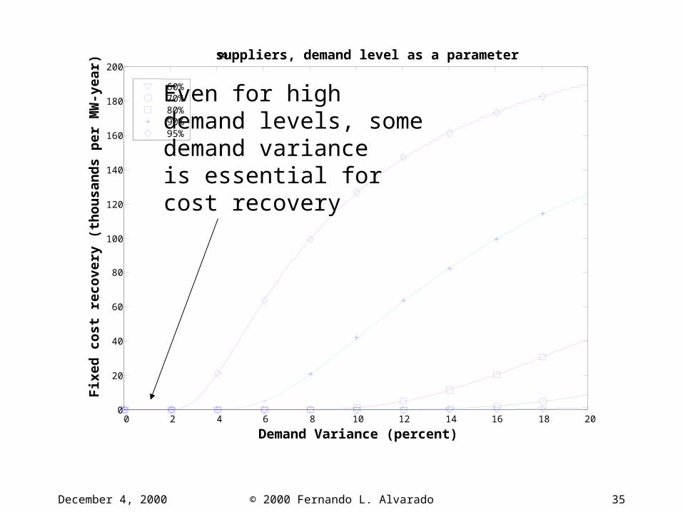
suppliers, demand level as a parameter
60%70%80%90%95%
Even for highdemand levels, somedemand varianceis essential forcost recovery

December 4, 2000 © 2000 Fernando L. Alvarado 36
0 2 4 6 8 10 12 14 16 18 200
50
100
150
200
250
Demand Variance (percent)
Fix
ed
co
st r
eco
very
(th
ou
san
ds
per
MW
-yea
r)
15 suppliers, demand level as a parameter
60%70%80%90%95%
For high enough demand levelscost recovery is possibleeven without demand variance

December 4, 2000 © 2000 Fernando L. Alvarado 37
0 2 4 6 8 10 12 14 16 18 200
50
100
150
200
250
300
Demand Variance (percent)
Fix
ed
co
st r
eco
very
(th
ou
san
ds
per
MW
-yea
r)
10 suppliers, demand level as a parameter
60%70%80%90%95%
For high demand levelsdemand variance can becomeirrelevant

December 4, 2000 © 2000 Fernando L. Alvarado 38
0 2 4 6 8 10 12 14 16 18 200
50
100
150
200
250
300
350
400
Demand Variance (percent)
Fix
ed
co
st r
eco
very
(th
ou
san
ds
per
MW
-yea
r)
6 suppliers, demand level as a parameter
60%70%80%90%95%
For low demand levels it isvery difficult to recoverfixed costs
December 4, 2000 © 2000 Fernando L. Alvarado 39
0 2 4 6 8 10 12 14 16 18 200
50
100
150
200
250
300
350
400
450
Demand Variance (percent)
Fix
ed
co
st r
eco
very
(th
ou
san
ds
per
MW
-yea
r)
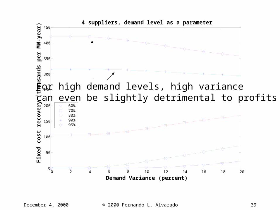
4 suppliers, demand level as a parameter
60%70%80%90%95%
For high demand levels, high variancecan even be slightly detrimental to profits

December 4, 2000 © 2000 Fernando L. Alvarado 40
0 2 4 6 8 10 12 14 16 18 200
50
100
150
200
250
300
350
400
450
Demand Variance (percent)
Fix
ed
co
st r
eco
very
(th
ou
san
ds
per
MW
-yea
r)
3 suppliers, demand level as a parameter
60%70%80%90%95%
With three or less suppliers, it becomes feasibleat high variances to recover fixed costs bywithholding at low demand

December 4, 2000 © 2000 Fernando L. Alvarado 41
0 2 4 6 8 10 12 14 16 18 200
5
10
15
20
25
30
35
40
45
50
Demand Variance (percent)
Fix
ed
co
st r
eco
very
(th
ou
san
ds
per
MW
-yea
r)
Demand level 60%, number of suppliers as a parameter
suppliers15 suppliers 10 suppliers 6 suppliers 4 suppliers 3 suppliers
At low demand and lowvariance it is impossibleto recover fixed costs

December 4, 2000 © 2000 Fernando L. Alvarado 42
0 2 4 6 8 10 12 14 16 18 200
20
40
60
80
100
120
Demand Variance (percent)
Fix
ed
co
st
rec
ov
ery
(th
ou
sa
nd
s p
er
MW
-ye
ar)
Demand level 70%, number of suppliers as a parameter
suppliers15 suppliers 10 suppliers 6 suppliers 4 suppliers 3 suppliers
At higher demand with 3 suppliersit is possible to recovercosts at low variance

December 4, 2000 © 2000 Fernando L. Alvarado 43
0 2 4 6 8 10 12 14 16 18 200
50
100
150
200
250
Demand Variance (percent)
Fix
ed
co
st
rec
ov
ery
(th
ou
sa
nd
s p
er
MW
-ye
ar)
Demand level 80%, number of suppliers as a parameter
suppliers15 suppliers 10 suppliers 6 suppliers 4 suppliers 3 suppliers
0 2 4 6 8 10 12 14 16 18 200
50
100
150
200
250
300
350
400
Demand Variance (percent)
Fix
ed
co
st
rec
ov
ery
(th
ou
sa
nd
s p
er
MW
-ye
ar)
Demand level 90%, number of suppliers as a parameter
suppliers15 suppliers 10 suppliers 6 suppliers 4 suppliers 3 suppliers
As demand increases, withholding becomesprofitable even when there are many suppliers

December 4, 2000 © 2000 Fernando L. Alvarado 44
0 2 4 6 8 10 12 14 16 18 200
50
100
150
200
250
300
350
400
450
Demand Variance (percent)
Fix
ed
co
st
rec
ov
ery
(th
ou
sa
nd
s p
er
MW
-ye
ar)
Demand level 95%, number of suppliers as a parameter
suppliers15 suppliers 10 suppliers 6 suppliers 4 suppliers 3 suppliers
Only in the caseof infinite suppliers is it
impossible to recover costs

December 4, 2000 © 2000 Fernando L. Alvarado 45
Comments on numeric results• The number of suppliers has a strong influence on cost
recovery– Below a certain number of suppliers, cost recovery by
withholding becomes easier
• There are demand threshold levels beyond which there is a jump in the ability to recover costs
• All studies assume that supplier can adjust level of withholding after learning the demand– Lower returns when this is not true, study underway
• Demand variance has a strong influence on ability to recover costs, sometimes with a threshold level
December 4, 2000 © 2000 Fernando L. Alvarado 46
Final remarks
• Two-technology suppliers can lead to higher than marginal prices as the knee of the supply curve is approached
• Larger number of suppliers reduces this effect• Market power studies should consider fixed
cost recovery issues• We did not even look at congestion or voltage
problems!


![La Chronica Gothorum Pseudo-Isidoriana (ms. Paris BN 6113) [Texto impreso] edición crítica, traducción y estudio, Fernando González Muñoz 2000](https://img.dokumen.tips/doc/110x75/55cf8631550346484b95337c/la-chronica-gothorum-pseudo-isidoriana-ms-paris-bn-6113-texto-impreso.jpg)


![O FERRO NA ESCULTURA PORTUGUESA DO …39 FC 2: Escultura do Penta Hotel [CONDUTO, Fernando – Conduto. Lisboa : 2000, p. 139.] FC 3: Escultura em Chaves [CONDUTO, Fernando – Conduto.Lisboa](https://img.dokumen.tips/doc/110x75/5fa5ca05f4ed1361ec2bba44/o-ferro-na-escultura-portuguesa-do-39-fc-2-escultura-do-penta-hotel-conduto-fernando.jpg)


