Embed Size (px)
Citation preview

Debt Rollover Risk, Credit Default Swap Spread and Stock Returns:
Evidence from the COVID-19 Crisis*
Ya Liu, Buhui Qiu, Teng Wang
First version: May 2020
This version: October 2020
Abstract
This paper studies how the COVID-19 shock affects the CDS spread changes and abnormal stock
returns of U.S. firms with different levels of debt rollover risk. We use the COVID-19 crisis as a
quasi-natural experiment of adverse cash flow shock that increases the default risk of firms facing
an immediate liquidity shortfall. We find that the COVID-19 shock significantly increased the
CDS spread and decreased the shareholder value for firms facing higher debt rollover risk. The
effect is stronger for firms that are non-financial, with higher volatility, and are more financially
constrained. Moreover, we find that firms with immediate refinancing needs suffered more than
firms with distant refinancing needs during the COVID-19 shock, which further confirms that
firms’ debt rollover risk is indeed a key factor that drives the heterogenous reactions to the shock.
The paper provides fresh insights into the role of firms’ debt rollover risk during the COVID-19
health crisis.
Keywords: Debt Rollover Risk; Credit Default Swap Spread; Stock Returns
* Ya Liu is affiliated to the University of Sydney, NSW 2006, Australia; Email: [email protected].
Buhui Qiu is affiliated to the University of Sydney, NSW 2006, Australia; Email: [email protected].
Teng Wang is affiliated to Board of Governors of the Federal Reserve System, Constitution Ave NW,
Washington DC 20551, USA; Email: [email protected]. The views expressed in this paper are solely
those of the authors and should not be interpreted as reflecting the views of the Board of Governors or the
staff of the Federal Reserve System
1
1. Introduction
The COVID-19 health crisis has caused significant disruptions to the economic activities around
the globe. Businesses of all sizes have been adversely affected due to both the lockdown imposed
by the local governments and the panic from local residence, causing a precipitous drop in
customer attendance rates. The health crisis creates a liquidity shock by triggering a sudden plunge
in firms’ cash flow, leaving those firms with little cash reserve and pressing financing needs
vulnerable to default. With unemployment rate skyrocketed to 14.7% within a few weeks’ time
and the unprecedented level of economic uncertainty due to the unpredictability of the COVID
pandemic, it is expected that a bankruptcy boom will arrive with default rates over the next twelve
months could rival or even exceed 2009 levels. In the event of actual bankruptcies, shareholders
can only claim the residual value of the firms, which often results in a total loss to the shareholder
value. How do investors react to the heightened bankruptcy risks at firms? Do firms facing
significant debt rollover risk (i.e., firms that have the immediate needs of repaying maturing debt
but may not have enough liquidity to meet the repayment obligation) suffer more from the health
crisis? These are very pressing questions to understand the economic impact of the pandemic. In
this paper, we use the COVID-19 crisis as a quasi-natural experiment of adverse cash flow shock
to investigate the effects of debt rollover risk on firms’ default risk and thus shareholder value.
The unprecedented health crisis provides a unique opportunity to study the heterogeneous
impact of debt rollover risk on firms’ default risk and shareholder value. The presence of capital
market frictions makes firms’ debt maturity structure matters (e.g., Diamond, 1991). The cash flow
shock induced by COVID-19 crisis exacerbates the rollover risks for firms having a large amount
of debt due shortly and insufficient cash reserves. First, the significant cash flow plunge caused by
the COVID-19 crisis makes it difficult for firms with large amount of debt maturing and little cash
2
reserves to meet its debt payment obligation and thus need to roll over their maturing debt to future
periods. Second, it is unclear ex ante whether such firms can rely on alternative sources for
refinancing given it is costly to acquire external financing through new equity or bond issuance
during the market downturns caused by COVID-19. Thus, without meaningful cash reserves,
borrower firms with a large amount of debt due shortly face significant debt rollover risk, as
lenders’ possible refusal to roll over the maturing debt (due to poor cash flows and huge
uncertainties) to future periods could force the borrower firms into default. If the cash reserve is
large enough to pay back the debt due, there is no need to roll the maturing debt over to future
periods. The literature also suggests that the negative impact of the Global Financial Crisis on firm
investment is more pronounced for firms with lower level of pre-cautionary cash reserves and
firms with more short-term debt outstanding (Duchin, Ozbas and Sensoy, 2010). Thus, we
construct a debt-rollover-risk measure based on the ratio of firms’ short-term debt (debt due within
one year) to cash and short-term investment before the crisis, and identify firms facing significant
debt rollover risk in the near future.
We focus on the credit default swap (CDS) spread changes and abnormal stock returns
when evaluating the heterogeneous market reactions to the shock. To the extent that the financial
markets are efficient enough to digest the potential effects from the shock, we will be able to
capture the heterogeneous impacts on firms’ default risk and shareholder value through these
measures. As firms with debt maturing shortly and insufficient cash reserve to pay off the maturing
debt may face severe debt rollover risk, their market measures are likely to react more strongly to
the shock. Similar to the Great Recession, the recent COVID-19 shock features a sudden collapse
in asset prices. With the S&P 500 stock price index dropping 34% within 33 days (from February
19 to March 23, 2020), the shock is severe enough to hit U.S. public firms unexpectedly. Although

3
COVID-19 shock is a systemic shock that affects the whole economy, the actual timing of the debt
due is different across various firms, causing different levels of rollover risk for firms at the time
of the COVID shock struck the market and thus the effects are likely to be more pronounced in
firms that face significant debt rollover risk.
Using data on firms’ CDS spread changes, we investigate whether the COVID-19 crisis
significantly increases the default probabilities of firms with significant debt rollover risk. Figure
1 shows the average cumulative 6-month CDS spread changes for the debt-rollover-risk quartiles.
Although CDS spread increases in February and March 2020 across all debt-rollover-risk quartiles,
the increase is much more prominent for firms in the highest rollover risk quartile—the cumulative
CDS spread change is a startling 900 basis points before declining subsequently. The cumulative
6-month CDS spread change for firms in the highest debt-rollover-risk quartile is more than four
times larger than the cumulative change for firms in the other three quartiles. We further examine
the cumulative 1-year, 5-year and 10-year CDS spread changes and document similar patterns, as
shown in Figures A1, A2 and A3 in the Appendix.
[Please insert Figure 1 here]
Our regression results also confirm that the COVID-19 shock exerts heterogeneous impact
on the default risk and CDS spread of firms with different levels of debt rollover risk. In particular,
we find that the shorter the CDS contract maturity, the greater is the increase in CDS spread for
firms with high debt rollover risk, indicating that investors are more concerned about the short-
term default risk for high rollover-risk firms than these firms’ long-term default risk. The COVID-
19 shock leads to an increase in CDS spread of 349 to 880 basis points across different CDS
contract maturities for firms in the highest rollover-risk quartile relative to firms in the other
rollover-risk quartiles. We also find that the impact of the COVID-19 crisis on CDS spread of high
4
rollover-risk firms is much more pronounced in the later sample period (from 3/2/2020 to
3/26/2020) when the U.S. gradually becoming the most COVID-19 affected country in the world
than in the first sample period (from 1/30/2020 to 2/28/2020) when the crisis mostly affecting Asia
and Europe. Additionally, we find that the impact of the shock on CDS spread of high rollover-
risk firms is much stronger if such firms also face tight financial constraints or have high firm
volatilities.
Since shareholders are the residual claimers of a firm’s assets once the firm defaults, an
increase in firms’ default risk negatively affects shareholder wealth. Consistent with the evidence
on default risk, we find that the crisis leads to significant negative abnormal stock returns for firms
with higher debt rollover risks. Figure 2 shows the average buy-and-hold abnormal stock returns
(BHARs) for different debt-rollover-risk quartiles over the sample period. Although the average
BHARs significantly decrease in general across all debt-rollover-risk quartiles in February and
March, the decline is more pronounced for the top two firm quartiles with the highest rollover risk.
[Please insert Figure 2 here]
Our regression results further confirm that relative to firms in the other quartiles of debt
rollover risk, the crisis leads to an economically significant decline of -2% to -3% in stock returns
for real-sector firms in the highest rollover-risk quartile over the sample period. Further, the lower
stock returns for high rollover-risk firms are confined to real-sector firms and not financial-sector
firms, and mainly concentrated in the later sample period when the U.S. becomes heavily impacted
by COVID-19. This finding is consistent with the notion that different from the Global Financial
Crisis, the COVID-19 crisis is a health crisis that directly hits the real sector and not the financial
sector businesses.1 In addition, we show that the negative stock return reactions are much stronger
1 The banking and financial industries are much better prepared when the COVID-19 crisis hit possibly also due to
the resilience built up through various post-Great Recession regulations.
5
for high debt-rollover-risk firms when such firms also face tight financial constraints, or have
higher stock return volatilities, consistent with the earlier findings from CDS spread changes and
the findings from the Global Financial Crisis (e.g., Ivashina and Scharfstein, 2011).
Our evidence that financial constraints amplify the magnitude of the impact of the COVID-
19 crisis on stock returns of high debt-rollover-risk firms is consistent with the implications from
the literature. For example, previous studies suggest that stock returns of financially constrained
firms tend to comove together, and such firms tend to earn higher returns on average (e.g., Whited
and Wu 2006). However, during crisis time, such firms tend to suffer more likely due to their
corporate liquidity shortfall. For example, Campbello, Graham, and Harvey (2010) find that during
the Global Financial Crisis, financially constrained firms planned deeper cuts in tech spending,
employment, and capital spending, burned through more cash, drew more heavily on lines of credit,
sold more assets to fund their operations, and bypassed attractive investment opportunities. The
evidence from our paper indicates that the liquidity shortfall due to the COVID-19 cash flow shock
exposes firms, especially those facing tight financial constraints, to debt rollover risk. Moreover,
the literature suggests that stock returns are primarily driven by firm’s cash flow news (e.g.,
Vuolteenaho, 2002). Our evidence that firm’s cash flow uncertainty amplifies the magnitude of
the impact of the COVID-19 crisis on stock returns of high debt-rollover-risk firms is consistent
with the implications from the literature. That is, firms with high cash flow uncertainty are likely
to be hit particularly hard by the cash flow shock of COVID-19 and thus should earn lower stock
returns during the crisis.
To strengthen the identification on the effects of rollover risk, we further zoom in on the
timing of firms’ debt rollover, and compare the effects of rollover risk on CDS spreads and BHARs
for firms with debt maturing immediately and firms with debt due later in the year. The key is to
6
understand that the actual timing of the COVID-19 strike is what makes it an exogeneous shock
to the firms. As the outbreak of the COVID-19 pandemic is entirely unexpected, the percentage of
firms’ debt that is maturing in the first few months of year 2020 when the COVID-19 shock hit
the U.S. is exogenous to firms’ choice ex ante. Even if the total amount of debt due in year 2020
is the same for two firms, the actual timing of the debt due is different, causing different levels of
rollover risk for firms at the time of the COVID-19 shock. The COVID-19 crisis creates a liquidity
shortfall by causing a sudden plunge in firms’ cash flow. If debt rollover risk is indeed a driver for
the heterogenous reactions in firms’ CDS spread and shareholder value, then we should expect a
stronger effect for firms that face immediate refinancing needs than for firms that face refinancing
needs in the second half of year 2020 (in other words, distant refinancing needs). Indeed, our
empirical results show that firms with immediate refinancing needs suffered more than firms with
distant refinancing needs during the COVID-19 cash flow shock. The results thus further confirm
the finding of our main tests. Finally, we perform various robustness tests including controlling
for new debt issuance in the first quarter of 2020, using alternative measures of debt rollover risk,
and separating the impact of the COVID-19 shock from that of the U.S. government relief package.
The results of these robustness tests are all consistent with our main findings and suggest that firms’
debt rollover risk is indeed a key factor that drives the heterogenous reactions to the COVID-19
shock.
This paper contributes to a few strands of literature. First, the paper contributes to the
literature on firms’ debt rollover risk. The extant literature highlights the importance of carefully
managing the risks from maturing debt (e.g. Froot, Scharfstein and Stein, 1993). Earlier research
on debt maturity choice discusses the trade-offs between having long-term versus short-term debt.
For example, the use of short-term debt overcomes underinvestment problems by mitigating the

7
conflicts of interest between managers, debt holders and equity holders (Myers 1977; Barclay and
Smith 1995), but exposes firms to rollover risks more often and heightens the chance of inefficient
liquidation (Diamond, 1991; He and Xiong, 2012). In the presence of credit market imperfections,
short-term debt can lower firm value if it has to be refinanced at an overly high interest rate (Froot,
Scharfstein and Stein, 1993; Sharpe, 1991; Titman, 1992). Looking at the Global Financial Crisis,
Almeida et al. (2012) demonstrate the adverse impact on investment for firms having large
proportion of debt maturing right after August 2007. Gopalan, Song and Yerramilli (2013) employ
a similar framework and find that firms with a large portion of debt maturing likely experience
credit downgrades and face higher spreads in the bond market.2
Our paper contributes to the literature on debt rollover risk in two important aspects. First,
our study provides fresh empirical evidence on the adverse effects of debt rollover risk on firm
default risk as reflected in the CDS spread and abnormal stock returns. Second, our study is the
first that looks at the adverse effects of debt rollover risk in a unique setting of the COVID-19
crisis. Differing from the Global Financial Crisis which first affected the financial market and
credit supply to firms, the COVID-19 health crisis directly affected firms’ cash flows. Stable cash
flows are not only essential for covering maturing debt but also crucial for raising new debt. Given
the unprecedented COVID-19 shock to cash flows, it is uncertain ex ante whether firms with large
amount of debt maturing and little cash reserves can successfully roll over their maturing debt.
This study takes advantage of the unique setting of the COVID-19 shock to study the impact of
debt rollover risk on corporate default and shareholder value.
2 A related stream of research looks at the granularity of the entire maturity structure of outstanding debt and provides
evidence on the availability and costs of financing (e.g., Norden, Roosenboom, and Wang 2016; Choi, Hackbarth, and
Zechner, 2018).
8
Moreover, the paper is related to the literature on the impact of economic shocks. The
literature shows that economic crises are associated with reductions in the aggregate output level
(e.g., Reinhart and Rogoff, 2008). Some studies examine the impact of the financial crises on banks
and show that there are significant negative effects on banks’ capital that reduces the supply of
loans to the corporate sector. Further evidence suggests that adverse consequences from increased
losses in the banking sector spill over to the corporate sector and negatively affect borrowing firms’
performance (Lemmon and Roberts, 2010; Chava and Purnanandam, 2011). This paper contributes
to the literature by documenting the heterogeneous effects of the COVID-19 shock on real-sector
firms and financial firms from a financial market perspective. Unlike the Global Financial Crisis,
the COVID-19 crisis is a health crisis that directly hits the real sector and not the financial sector.
The paper is also related to research on firms’ holding of cash reserves. Many empirical
papers on corporate liquidity management focus on cash and short-term investment as an important
source of liquidity in the presence of market frictions. For example, financially constrained firms
may benefit from holding cash that mitigates the underinvestment problem (e.g., Opler et al. 1999;
Almeida, Campello and Weisbach, 2004; Faulkender and Wang, 2006; Denis and Sibilkov, 2010;
Duchin, Ozbas and Sensoy, 2010). However, in firms with agency problems, holding cash provides
the chance for managers to engage in value-destroying investment activities (Jensen, 1986;
Harford, 1999). Thus, holding excess cash reserve is regarded as expensive in practice (Holmstrom
and Tirole, 2000, 2001). This paper contributes to the literature by emphasizing the importance of
holding enough cash reverses to mitigate the rollover risks under the context of the COVID-19
health crisis.

9
Last but not least, this paper relates to the contemporaneous work on the market reaction
to COVID-19 crisis for firms.3 For instance, Ramelli and Wagner (2020) find that investors were
moving away from U.S. firms with exposures to China when the virus was contained in China.
Moreover, when the virus spread to Europe and the U.S., leverage ratio and cash holding are
important value drivers as they have significant negative and positive effects on stock prices
respectively. Ding, Levine, Lin and Xie (2020) investigate the stock market reactions of firms
around the world in the early 2020. They find that the drop in stock price was milder for firms with
stronger pre-2020 finances, less exposure to COVID-19 through global supply chains and
customer locations, more CSR activities, and less entrenched executives. Focusing on non-
financial firms during the COVID-19 crisis, Fahlenbrach, Rageth, and Stulz (2020) find a worse
decline in stock prices for firms with less cash reserves, and firms with more short-term or long-
term debt. The difference between the effects of short-term and long-term debt is insignificant.
The authors also find levered firms experienced stronger increase in the CDS premiums but do not
find firms with more short-term debt to be affected differently from firms with more long-term
debt. In addition, they find that the decline in the stock prices was not affected by firms’ ability of
accessing financial markets as measured by the financial constraint indices prior to the crisis.
Alfaro, Chari, Greenland and Schott (2020) find that an unanticipated doubling (halving) of
projected COVID-19 infections forecasts next-day decreases (increases) in aggregate US stock
market value of 4 to 11 percent, and firms with higher leverage, lower profitability or higher capital
intensity experienced worse COVID-19 related losses. These contemporaneous papers on the
market reactions during the COVID-19 crisis do not focus on the effects of debt rollover risk as
3 There are many contemporaneous papers that are broadly related to the impact of COVID-19 crisis, but not on the
effects on the financial markets (e.g., Acharya and Steffen, 2020; Cejnek, Randl and Zechner, 2020; Halling, Yu and
Zechner, 2020; Li, Strahan and Zhang, 2020; Bartik, Cullen, Glaeser, Luca and Stanton, 2020; Baker, Farrokhnia,
Meyer, Pagel and Yannelis, 2020).
10
we do. In this paper, we look at both financial and real-sector firms with immediate financing needs
and distant financing needs of rolling over debt at the time of COVID-19 shocks. Facing an
immediate liquidity shortfall as implied by the COVID-19 crisis, we document a substantial
increase in CDS spread changes and decline in stock returns for firms with higher levels of debt
rollover risk. We also find that being financially constrained or having greater firm volatilities
makes these firms with higher rollover risks suffered more from the COVID-19 crisis.
The rest of the paper proceeds as follows. Section 2 describes data and explains how we
measure debt rollover risk and market reactions. Section 3 investigates the relation between debt
rollover risk and CDS spread changes during the COVID-19 crisis. Section 4 examines the relation
between debt rollover risk and abnormal stock returns during the crisis. Section 5 investigates
whether firms with immediate refinancing needs suffered more during the COVID-19 cash flow
shock. Section 6 reports the results from various robustness tests. Section 7 concludes.
2. Background and Data
2.1. COVID-19 Crisis in the United States
The COVID-19 pandemic, also known as the coronavirus pandemic, is an ongoing pandemic of
coronavirus disease, caused by severe acute respiratory syndrome coronavirus 2 (SARS-CoV-2).
The outbreak was first identified in Wuhan, China, in December 2019. The virus then quickly
spread across the globe, and the U.S. too was hard hit by the COVID-19 crisis in early of 2020.
After the first death in the United States was reported in Washington state on February 29,
Governor Jay Inslee declared a state of emergency, an action soon followed by other states.
President Trump then declared a national emergency on March 13, making federal funds available
to respond to the crisis. As of May 17, 2020, more than 4.71 million cases of COVID-19 have been
reported in more than 188 countries and territories, resulting in more than 315,000 deaths. The

11
outbreak of COVID-19 pandemic has far-reaching consequences on the society than the spread of
the deadly disease itself. Various levels of mandatory shutdowns and social distancing measures
implemented by local and states governments have brought many parts of the U.S. economy to a
standstill. In April alone, nearly a quarter of residents (renters and homeowners) did not pay full
housing costs. Many workers were furloughed or laid off as a result of business and school closures
and the cancellation of public events. According to data released by the U.S. Bureau of Labor
Statistics on May 8, the U.S. economy lost a staggering record 20.5 million jobs in April, pushing
the unemployment rate to 14.7%—the highest monthly rate since record keeping began in 1948.
2.2. Data and Variables
We measure firms’ stock price reactions and CDS spread changes over the entire sample period
from 1/30/2020 to 3/26/2020. We also separately examine two subperiods: 1/30/2020-2/28/2020
and 3/2/2020-3/26/2020.4 The sample period and subperiods are based on three major milestones
related to the development of COVID-19 crisis, including 1/30/2020, the date when the World
Health Organization (WHO) declared a global public-health emergency, 2/29/2020, the date when
the US reports the first death on American soil, and 3/26/2020, the date when the U.S. became the
world’s most affected country—total confirmed cases in the US reached 82,404 on this date,
surpassing China’s 81,782 and Italy’s 80,589.5
To analyze the stock market reactions, we obtain daily stock price data of all common
stocks (CRSP share code 10 or 11) listed on NYSE, AMEX, and NASDAQ from the Center for
Research in Security Prices (CRSP). We obtain information on firms’ CDS spread from Markit
4 2/29/2020 and 3/1/2020 are weekends with no trading activities. 5 The two-trillion-dollar relief package passed the U.S. Senate on March 25th and the House of Representatives on
March 27th. It was then immediately signed into law by President Trump on March 27th. News about the rescue package
sent the S&P 500 index up by 9.38% on March 24—its best day since Oct 28, 2008. The market has generally been
in an upward trend since then. Our results are even stronger if our sample period stops on March 23 rd.
12
database for firms with CDS contracts of various maturities. Only the CDS contracts on public
firms for which we have data in CRSP and COMPUSTAT are used in our study. To control for
firm characteristics, we obtain one-quarter lagged financial data from Compustat. We then link
firms’ stock price and CDS reactions to firms’ characteristics such as rollover risk in the quarter
prior to the COVID crisis to study the cross-sectional variation in the market reactions to the
shocks. We also include standard firm-level control variables such as firm size (Size), profitability
(Roa), firm market-to-book equity ratio (MTB), leverage ratio (Leverage), past stock returns of the
firm (Past_Return) and past volatility of stock returns (Vol) as it is well known that these firm
characteristics are related to cross-sectional stock returns.
We measure the potential impact of debt rollover risk based on the ratio of firms’ debt that
matures shortly (due within one year) to cash and short-term investment before the crisis
(DD_One). Having a larger percent of debt maturing shortly subjects a firm to liquidity risks of
creditors’ refusing to roll over the debt due to the cash flow shock imposed by the COVID-19
crisis.6 And having abundant cash reserves help mitigate the adverse effects from potentially not
being able to roll over the debt due. If the cash reserve is large enough to pay back the debt due,
there is no need to roll the debt over to future periods. The literature also suggests that the negative
impact of the Global Financial Crisis on firm investment is more pronounced for firms with lower
level of pre-cautionary cash reserves and firms with more short-term debt outstanding (Duchin,
Ozbas and Sensoy, 2010). A higher value of this ratio thus indicates higher potential effects from
debt rollover risk. In other words, firms with immediate needs of repaying maturing debt and
insufficient cash reserves will face significant debt rollover risk. In the robustness tests, we also
6 Corporate cash flows are one of the key factors considered by banks when they structure terms on new loans and
renegotiating existing loans, and cash flow covenants are one of the most widely used types in lines of credit (e.g.,
Roberts and Sufi, 2009; Sufi, 2009).
13
construct two alternative debt-rollover-risk measures by scaling the amount of debt due within one
year with the amount of total debt outstanding (Friewald, Nagler and Wagner, 2018) and the
amount of total long-term debt outstanding (Almeida et al., 2012; Hu, 2010), respectively.
Our dataset consists of 3,047 firm observations with non-missing stock returns and
financial data. Then, we create a subsample that contains 234 firms having CDS contracts with
non-missing main spread data in Q1 2020. Table A1 provides the detailed definition and data
source for each of the variables used in the study and Table 1 provides the summary statistics. All
continuous variables are winsorized at the 1st and 99th percentiles to limit the influence of outliers.
[Please insert Tables 1 here]
3. Debt Rollover Risk and CDS Spread during the COVID-19 Crisis
This section investigates how the COVID-19 shock affects the CDS spread of firms with different
levels of debt rollover risk. We also examine whether financial constraints and firm volatilities
amplify the impact of the COVID-19 shock on the default risk and CDS spread of high debt-
rollover-risk firms.
3.1. Debt Rollover Risk and CDS Spread
We sort firms with available CDS spread data (i.e., 234 firms) equally into quartiles according to
their debt rollover risk (DD_One) and construct an indicator variable, DD_One_High25, which
equals 1 if the firm falls in the top quartile of debt due within one year scaled by cash and short-
term investment (with available CDS data) and equals 0 otherwise. We then employ the following
regression model to examine the impact of the COVID-19 shock on CDS spread of firms with
different levels of debt rollover risk:
𝑆𝑝𝑟𝑒𝑎𝑑𝑖 = 𝛼 + 𝛽1𝐷𝐷_𝑂𝑛𝑒_𝐻𝑖𝑔ℎ25𝑖 + 𝛽2𝐶𝑜𝑛𝑡𝑟𝑜𝑙𝑠𝑖 + 𝐼𝑛𝑑𝑢𝑠𝑡𝑟𝑦_𝐹𝐸 + 𝜀𝑖,𝑡 . (1)
14
In Equation (1), the dependent variable, Spread, is the change in firm i’s 6-month, 1-year,
5-year or 10-year CDS spread over the sample period (CDS_6M, CDS_1Y, CDS_5Y or CDS_10Y).
The regression coefficient of DD_One_High25 reflects the incremental impact of the crisis on
firms in the highest debt-rollover-risk quartile relative to firms in the other quartiles. Control
variables include firm characteristics such as firm size (Size), profitability (Roa), market-to-book
equity ratio (MTB), financial leverage (Leverage), past stock returns (Past_Return), stock return
volatility (Vol) and stock illiquidity (Illiquidity). Industry fixed effects (i.e., 2-digit SIC industry
indicators) are included to control for potential heterogeneous responses of firms from different
industries.7 Standard errors are clustered at the 2-digit SIC industry level. The results are reported
in Table 2.
[Please insert Table 2 here]
We separately estimate Equation (1) for the first period from 1/30/2020 to 2/28/2020 (i.e.,
the period from the date when WHO declares a global public-health emergency to the date when
the U.S. reports the first death on American soil), the second period from 3/2/2020 to 3/26/2020
(i.e., the period when the U.S. gradually develops into the most COVID-19 affected country in
terms of the number of cases identified), and the full sample period from 1/30/2020 to 3/26/2020
and report the results in Panels A, B, and C respectively. Panel A of Table 2 shows that the
regression coefficients of DD_One_High25 are significantly positive at the 1% level across
different regression models with CDS_6M, CDS_1Y, CDS_5Y and CDS_10Y as the dependent
variables respectively. The results indicate that relative to firms in the other quartiles of debt
rollover risk, the COVID-19 crisis leads to an economically significant increase in CDS spread of
7 For example, firms from transportation industries may react very differently from internet or online gaming firms.

15
104 to 207 basis points across different CDS contract maturities for firms in the highest rollover-
risk quartile in the first period when the US reports the first death on American soil.
Panel B shows even more significant results in the second period. Again, the regression
coefficients of DD_One_High25 are significantly positive across different regression models. The
results indicate that the crisis leads to a startling increase in CDS spread of 270 to 673 basis points
across different CDS contract maturities for firms in the highest rollover-risk quartile relative to
firms in the other rollover-risk quartiles. Moreover, the shorter the CDS maturity, the larger is the
increase in CDS spread, indicating that investors are more concerned about the short-term default
risk for high rollover-risk firms than these firms’ long-term default risk.
Panel C shows the impact of the COVID-19 crisis on the CDS spread of firms with different
levels of debt rollover risk over the entire sample period from 1/30/2020 to 3/26/2020. Consistent
with the earlier results, the results in Panel C suggest that the COVID-19 crisis leads to an increase
in CDS spread of 349 to 880 basis points across different CDS contract maturities for firms in the
highest rollover-risk quartile relative to firms in the other rollover-risk quartiles—again, the shorter
the CDS maturity, the greater is the impact. The regression coefficients of three control variables,
Roa, Past_Return and Vol, are also statistically significant, indicating that firms with lower past
stock returns, greater stock return volatility or greater profitability experience greater increase in
CDS spread during the COVID-19 crisis.
As a robustness test, we use the first (lowest) rollover-risk quartile as the reference group
and construct three indicator variables, including DD_One_Group2, DD_One_Group3, and
DD_One_Group4, to indicate the other three quartiles and re-estimate Equation (1). The results
are reported in Table A2 in the Appendix. We consistently find that only the regression coefficient
of the highest rollover-risk quartile (DD_One_Group4) is significantly positive across different
16
regression models with CDS_6M, CDS_1Y, CDS_5Y and CDS_10Y as the dependent variables
respectively in the first, second and whole periods. The results indicate that relative to firms in the
lowest debt-rollover-risk quartile, firms in the highest debt-rollover-risk quartile on average
experience a highly significant increase in CDS spread of 353 to 974 basis points over the full
sample period. Moreover, the increase in CDS spread is much more pronounced in the second
period than in the first period.
To summarize, we find that the COVID-19 shock exerts heterogeneous impact on the
default risk and CDS spread change of firms with different levels of debt rollover risk. The crisis
leads to a sharp increase in CDS spread for firms in the highest debt-rollover-risk quartile relative
to firms in the other quartiles—the shorter the maturity of the CDS contract, the greater is the
increase in CDS spread for firms with high debt rollover risk. Furthermore, the impact is much
more pronounced in the second period than in the first period.
3.2. Debt Rollover Risk and CDS Spread Conditional on Financial Constraints or Firm Volatilities
Given that the COVID-19 crisis posts a significant hit to firm cash flow, it may be particularly
challenging for a financially constrained firm with little cash reserves and large amount of debt
due in the near future to meet its payment obligation, resulting in significant default risk. Literature
suggests that stock returns of financially constrained firms tend to comove together, and such firms
tend to earn higher returns on average (e.g., Whited and Wu 2006). However, during crisis time,
such firms tend to suffer more likely due to their corporate liquidity shortfall (e.g. Campbello,
Graham, and Harvey, 2010). We expect the negative cash flow shock due to the COVID-19 crisis
to increase the default risk for high debt-rollover-risk firms particularly when these firms also face
tight financial constraints. In other words, financial constraints can amplify the impact of the
COVID-19 shock on the default risk and CDS spread of high debt-rollover-risk firms.

17
We thus partition the sample firms with available CDS spread data (i.e., 234 firms) into
high- and low-constraint groups based on six commonly used financial-constraint measures: 1) the
Hadlock and Pierce (2010) index (HP), 2) the Whited and Wu (2006) index (WW), 3) the Altman’s
Z score (Z_Score), 4) the Kaplan and Zingales (1997) index (KZ), 5) whether the firm paid any
cash dividend over the past fiscal year (Non_Div), and 6) Whether the firm’s Standard & Poor’s
(S&P) long-term debt is rated below investment grade (Non_Invest_Grade). For each of the first
four financial-constraint measures, the indicator variable, High_FC, equals 1 for firms with
greater-than-sample-median financial constraints and equals 0 otherwise. For the fifth measure,
High_FC equals 1 if the Non_Div indicator (which takes the value of 1 if the firm did not pay any
cash dividend in 2019) equals 1 and equals 0 otherwise. For the sixth measure, High_FC equals 1
if the Non_Invest_Grade indicator (which takes the value of 1 if the firm’s long-term debt is rated
below investment grade by S&P) equals 1 and equals 0 otherwise. We then interact High_FC with
the DD_One_High25 indicator in CDS spread regressions.8 Component terms of the interaction
terms (i.e., High_FC and DD_One_High25) are also included in the regressions. Moreover, we
include the firm-level control variables and industry fixed effects as in Table 2. The results are
reported in Table 3. For brevity concern, we only report the regression results using 6-month CDS
spread (CDS_6M) as the dependent variable in the full sample period (as the results with other
CDS maturities and with the first and second subperiods are qualitatively similar to the reported
results) and only report the regression coefficients of the interaction terms (which are our main
interest).
[Please insert Table 3 here]
8 We further check and find that the high- and low-constraint firms are allocated quite evenly into the different debt-
rollover-risk quartiles.

18
Panel A of Table 3 shows that the regression coefficients of the interaction terms
DD_One_High25*High_FC are significantly positive and large in magnitude across all
regressions with different financial-constraint measures. The results suggest that the COVID-19
shock increases the CDS spread for the firms in the top quartile of debt rollover risk relative to
firms in the other rollover-risk quartiles by an incremental 1,157 to 3,575 basis points over the full
sample period if these high-rollover-risk firms also face tight financial constraints.9 Thus, our
empirical results confirm that the negative cash flow shock occasioned by the COVID-19 crisis
significantly increases the default risk and CDS spread for high debt-rollover-risk firms
particularly when such firms also face tight financial constraints.
It is known that firms with greater volatilities tend to have greater default risk and CDS
spread (Ericsson, Jacobs and Oviedo, 2009). Thus, we further conjecture that the negative cash
flow shock occasioned by the COVID-19 crisis should significantly increase the default risk for
high debt-rollover-risk firms especially if such firms also have high volatilities prior to the crisis.
That is, high volatilities can also amplify the impact of the COVID-19 shock on the CDS spread
of firms with high debt rollover risk.
We next partition the sample firms with available CDS spread data equally into high- and
low-volatility groups based on their past total stock return volatility (Vol), idiosyncratic stock
return volatility (Ivol), options-implied volatility (Impl_Vol),10 ROA volatility (Roa_Vol), and
operating cash flow volatility (Operating_Cash_Vol) respectively. For each of these volatility
measures, we construct an indicator variable High_Vol, which equals 1 for firms with greater-than-
9 In Panel A of Table A3 in the Appendix, instead of interacting High_FC only with DD_One_High25, we interact
High_FC with three different debt-rollover-risk indicators (i.e., DD_One_Group2, DD_One_Group3, and
DD_One_Group4) in CDS spread regressions. The results are qualitatively similar to those in Panel A of Table 3. 10 Options-implied volatility is a market-based, forward-looking measure of firm stock return volatility (e.g.,
Christensen and Prabhala, 1998; Fleming, Kirby and Ostdiek, 1998; Busch, Christensen and Nielsen, 2011; Guo and
Qiu, 2014).
19
sample-median level of volatility and equals 0 otherwise. We then interact High_Vol with the
DD_One_High25 indicators in CDS spread regressions.11 Component terms of the interaction
terms, firm-level control variables and industry fixed effects are also included in the regressions.
The results are reported in Panel B of Table 3. For brevity concern, again we report only the
regression results using 6-month CDS spread (CDS_6M) as the dependent variable in the full
sample period (the results with other CDS maturities and with the first and second subperiods are
qualitatively similar to the reported results) and only report the regression coefficients of the
interaction terms.
Consistent with our expectation, Panel B of Table 3 shows that the coefficients of the
interaction terms DD_One_High25*High_Vol are positive and statistically significant across all
five regressions. The results indicate that the COVID-19 shock increases the CDS spread for the
firms in the top quartile of debt rollover risk relative to firms in the other rollover-risk quartiles by
an incremental 1,443-2,290 basis points over the full sample period if these high-rollover-risk
firms also have high volatilities.12 Therefore, our empirical results strongly support the conjecture
that the negative cash flow shock occasioned by the COVID-19 crisis significantly increases the
default risk and CDS spread for high debt-rollover-risk firms particularly if such firms also have
high stock return or cash flow volatilities.
4. Debt Rollover Risk and Stock Returns during the COVID-19 Crisis
In the last section, we document that the COVID-19 shock significantly increases the default risk
and CDS spread of firms with high debt rollover risk. Because a sharp increase in default risk
11 We check that high- and low-volatility firms are allocated quite equally into different debt-rollover-risk quartiles. 12 In Panel B of Table A3 in the Appendix, instead of interacting High_Vol only with DD_One_High25, we interact
High_Vol with three different debt-rollover-risk indicators (i.e., DD_One_Group2, DD_One_Group3, and
DD_One_Group4) in CDS spread regressions. The results are very similar to those in Panel B of Table 3.
20
should significantly decrease the firm’s equity value, we next examine how the COVID-19 shock
affects stock returns of firms with different levels of debt rollover risk.
4.1. Debt Rollover Risk and Stock Returns
We first use the event study approach to discern the impact of the COVID-19 shock on stock
returns of firms with different levels of debt rollover risk. The sample consists of 3,047 firms with
non-missing stock return data from CRSP and financial data from Compustat. We sort the sample
firms equally into quartiles according to their levels of debt due within one-year scaled by cash
and short-term investment (DD_One). For each firm, we then calculate its buy and hold abnormal
stock returns (BHARs) and cumulative abnormal returns (CARs) for three periods: 1) 1/30/2020
– 2/28/2020 (the first period); 2) 3/2/2020 – 3/26/2020 (the second period); and 3) 1/30/2020 –
3/26/2020 (the full period) similar to Table 2. We use the S&P 500 stock market index as the
market portfolio. We calculate CARs using both the market model and the market-adjusted model.
The market-model estimation window is days (-150, -50) before 1/30/2020. The event-study
results are reported in Table 4.
[Please insert Table 4 here]
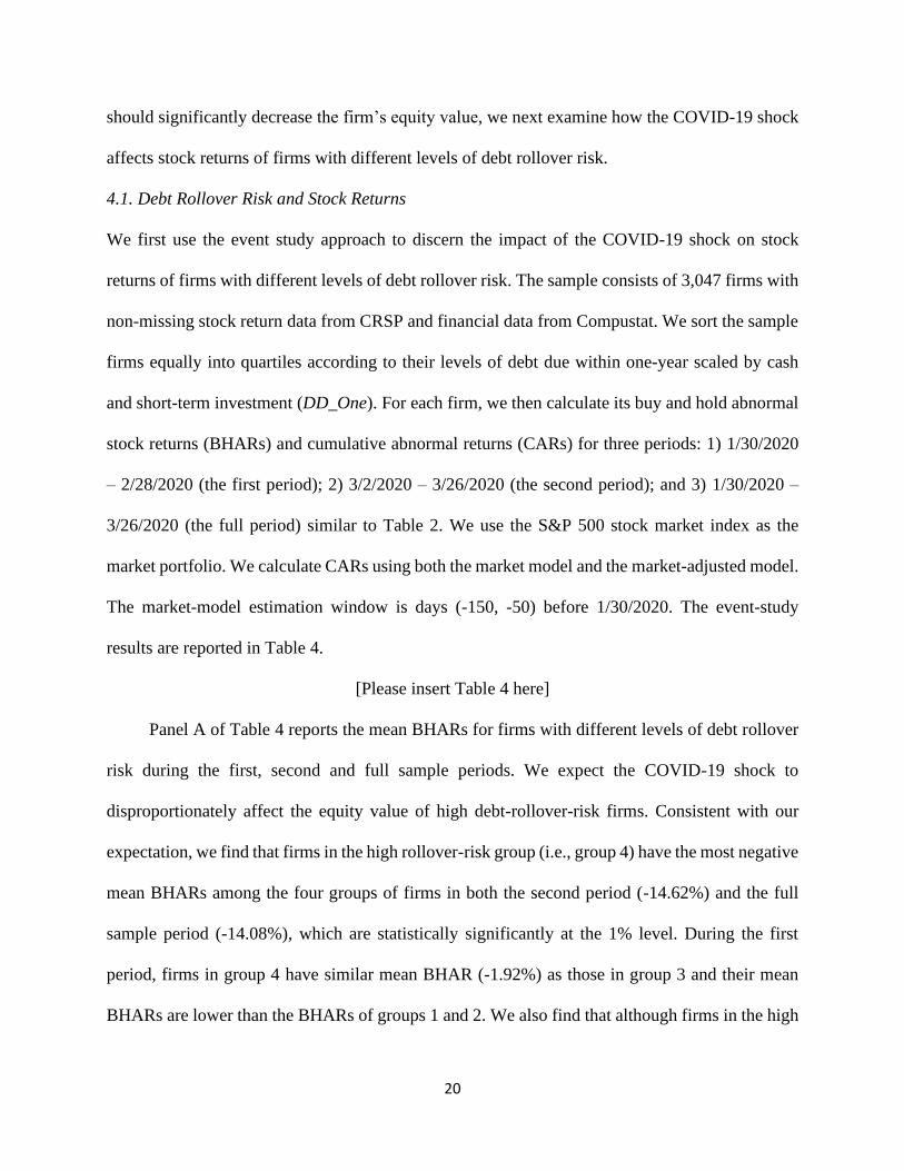
Panel A of Table 4 reports the mean BHARs for firms with different levels of debt rollover
risk during the first, second and full sample periods. We expect the COVID-19 shock to
disproportionately affect the equity value of high debt-rollover-risk firms. Consistent with our
expectation, we find that firms in the high rollover-risk group (i.e., group 4) have the most negative
mean BHARs among the four groups of firms in both the second period (-14.62%) and the full
sample period (-14.08%), which are statistically significantly at the 1% level. During the first
period, firms in group 4 have similar mean BHAR (-1.92%) as those in group 3 and their mean
BHARs are lower than the BHARs of groups 1 and 2. We also find that although firms in the high

21
rollover-risk group generally have the lowest BHARs, the relation between mean BHAR and debt
rollover risk is not monotonic in the first three groups—firms in group 2 have higher mean BHARs
than firms in the other two groups. The significantly negative average BHARs for all sample firms
during the first, second and full sample periods suggest that small firms generally fare worse than
large firms during the COVID-19 crisis. Results are qualitatively similar when we examine CARs
estimated using the market model (Panel B) and the market-adjusted model (Panel C). In particular,
firms with high debt rollover risk (group 4) generally have the lowest CARs among the four debt-
rollover-risk groups during the COVID-19 crisis.
Next, we use the following regression specification to examine the impact of the COVID-
19 shock on stock returns of firms with different levels of debt rollover risk:
𝑅𝑒𝑡𝑢𝑟𝑛𝑖 = 𝛼 + 𝛽1𝐷𝐷_𝑂𝑛𝑒_𝐻𝑖𝑔ℎ25𝑖 + 𝛽2𝐶𝑜𝑛𝑡𝑟𝑜𝑙𝑠𝑖 + 𝐼𝑛𝑑𝑢𝑠𝑡𝑟𝑦_𝐹𝐸 + 𝜀𝑖,𝑡 . (2)
In Equation (2), the dependent variable, Return, is the BHAR or CAR of firm i in the first,
second or full sample period. DD_One_High25 equals 1 if firm i’s debt rollover risk falls in the
highest quartile of 3,047 sample firms with available stock returns and financial data and equals 0
otherwise. Similar to Equation (1), the regression coefficients of DD_One_High25 reflect the
incremental impacts of the crisis on firms in the highest debt-rollover-risk quartile relative to firms
in the other quartiles. Control variables include firm size (Size), profitability (Roa), market-to-
book equity ratio (MTB), financial leverage (Leverage), past stock returns (Past_Return), stock
return volatility (Vol), stock illiquidity (Illiquidity), and industry fixed effects (i.e., 2-digit SIC
industry indicators). Standard errors are again clustered at the 2-digit SIC industry level. The
results are reported in Table 5. For brevity, we report only the results using BHAR as the dependent
variable (as results using CAR as the dependent variable are qualitatively very similar to the
reported results).

22
[Please insert Table 5 here]
We separately report the results of estimating Equation (2) for real-sector firms, banking
and financial firms and the full sample in Panels A, B and C of Table 5, respectively.13 Panel A
shows that while the regression coefficients of DD_One_High25 are insignificantly negative in
the first period (Columns 1 and 2), they are significantly negative in the second and the full periods
(Columns 3 to 6)—comparing with firms in the other debt-rollover-risk quartiles, high rollover-
risk firms on average produce significantly lower BHARs by 2-3% during the COVID-19 crisis
(mainly due to their low returns in the second period). This finding is consistent with our earlier
findings on the CDS spread changes of firms with high debt rollover risk.
In terms of control variables, the regression coefficients of Size, MTB, Past_Return, and
Illiquidity are significantly positive, while those of Leverage and Vol are significantly negative.
This finding indicates that larger firms and firms with higher valuation, better past stock
performance or lower stock liquidity fare better, while firms with greater leverage or more volatile
past stock returns fare worse, during the COVID-19 crisis.
Panel B shows the regression results for banking and financial firms. Interestingly, we find
that the regression coefficients of high debt rollover risk are statistically insignificant in general.
This finding suggests that the uncovered heterogeneous effect of the COVID-19 shock on firms
with different levels of debt rollover risk is mainly concentrated in the main-street firms. Different
from the Global Financial Crisis, which is a financial crisis first starting from the banking and
financial industries and then spreading to the real sector through the decrease in credit supply, the
COVID-19 crisis is a health crisis that directly hits the real sector and not the financial sector.
13 It is valuable to compare the CDS spread changes between the real-sector and financial firms. However, we are
constrained by the limitation of the CDS data––only 20+ financial firms have complete and non-missing data on CDS
spreads. Thus, it is challenging to draw general conclusions on the comparison between the financial and real-sector
firms when it comes to the effects of the COVID-19 on CDS spread changes.

23
Moreover, the banking and financial industries are much better prepared when the COVID-19
crisis hit, possibly also due to the resilience built up through various post-global-financial-crisis
regulations (e.g., the Dodd-Frank Act, the stress tests, etc.). Thus, the finding that the uncovered
effect is mainly concentrated in the real sector is perhaps not too surprising.
Panel C shows the regression results using the full sample of both real-sector and financial-
sector firms. The results are qualitatively similar to, but understandably weaker than, those
reported in Panel A. We generally find that firms in the highest rollover-risk quartile produce lower
stock returns than firms in the other rollover-risk quartiles during the crisis.
To ensure the robustness of the findings, we use the first (lowest) rollover-risk quartile as
the reference group and construct three indicator variables, including DD_One_Group2,
DD_One_Group3, and DD_One_Group4, to indicate the other three rollover-risk quartiles and
reestimate Equation (2). The results are reported in Table A4 in the Appendix. Panel A of Table
A4 shows the regression results for real-sector firms, which are qualitatively similar to those
reported in Panel A of Table 5. The regression coefficients of DD_One_Group4 are negative
across all the six regressions and significantly so in the latter four regressions. The results indicate
that relative to firms in the lowest rollover-risk quartile, firms in the highest debt-rollover-risk
quartile on average produce significantly lower BHARs by around 2.5-3% during the full sample
period. Moreover, the low stock returns of high rollover-risk firms are mainly concentrated in the
second period. Panels B and C of Table A4 also show qualitatively similar results as those reported
in Panels B and C of Table 5. In particular, the heterogeneous impact of the COVID-19 shock on
firms with different levels of debt rollover risk is mainly confined to the real sector and not the
financial sector.14
14 Consistent with the results in Table 4 (that firms in the second rollover-risk quartile have the highest returns during
the crisis), Panel C of Table A4 shows that the coefficient of DD_One_Group2 is positive in all regression models
24
To summarize, we find that the COVID-19 shock exerts heterogeneous impact on stock
returns of firms with different levels of debt rollover risk. Consistent with the patterns depicted in
Figure 2, the crisis leads to a significantly lower stock returns for firms with high debt rollover risk
than other firms—the finding is mainly driven by real-sector firms and not financial-sector firms
and mainly concentrated in the second period (when the U.S. becomes heavily impacted by the
health crisis).
4.2. Debt Rollover Risk and Stock Returns Conditional on Financial Constraints or Firm
Volatilities
In earlier results, we document that financial constraints amplify the impact of the COVID-19
shock on the default risk and CDS spread of high debt-rollover-risk firms. In this section, we
similarly examine whether financial constraints affect the magnitude of the impact of the COVID-
19 shock on stock returns of high debt-rollover-risk firms.
We partition the sample firms with available stock returns and financial data (i.e., 3,047
firms) into high- and low-constraint groups based on the following six financial-constraint
measures: 1) the Hadlock and Pierce (2010) index (HP), 2) the Whited and Wu (2006) index (WW),
3) the Altman’s Z score (Z_Score), 4) the Kaplan and Zingales (1997) index (KZ), 5) whether the
firm paid any cash dividend over the past fiscal year (Non_Div), and 6) Whether the firm’s
Standard & Poor’s (S&P) long-term debt is rated below investment grade (Non_Invest_Grade).
For each of these measures, we then similarly construct the indicator variable High_FC to indicate
firms facing tight financial constraints. We then interact High_FC with the DD_One_High25
indicator in stock return regressions. Component terms of the interaction term (i.e., High_FC and
and significantly so in five out of six regression models—although firms in both the first and second rollover risk
quantiles have low debt rollover risk, firms in the second rollover risk quartile on average have higher BHARs than
firms in the first quartile by around 2-2.5% in the whole period.

25
DD_One_High25), firm-level control variables and industry fixed effects are included in all
regressions. The results are reported in Table 6. For brevity concern, we only report the regression
results using BHAR as the dependent variable in the full sample period and only report the
regression coefficient of the interaction term.
[Please insert Table 6 here]
Panel A of Table 6 shows that the regression coefficients of the interaction terms
DD_One_High25*High_FC are negative in all regressions and significantly so in three out of the
six regressions. The results suggest that the COVID-19 shock decreases stock returns for the firms
in the top quartile of debt rollover risk relative to firms in the other rollover-risk quartiles by an
incremental 2-4% over the full sample period if these high-rollover-risk firms also face tight
financial constraints according to the financial-constraint measures of HP, Z-Score, and KZ. Thus,
consistent with the earlier CDS spread finding, we find that the COVID-19 shock significantly
decreases stock returns for firms with high debt rollover risk particularly when these firms also
face tight financial constraints.15
As our earlier findings suggest that high firm volatilities amplify the impact of the COVID-
19 shock on the default risk and CDS spread of high debt-rollover-risk firms, we further examine
whether firm volatilities similarly amplify the impact of the COVID-19 shock on stock returns of
such firms. We again partition the sample firms with available stock returns and financial data
equally into high- and low-volatility groups based on their past total stock return volatility (Vol),
idiosyncratic stock return volatility (Ivol), options-implied volatility (Impl_Vol), ROA volatility
(Roa_Vol), and operating cash flow volatility (Operating_Cash_Vol). For each of these volatility
15 In Panel A of Table A5 in the Appendix, instead of interacting High_FC only with DD_One_High25, we interact
High_FC with three different debt-rollover-risk indicators (i.e., DD_One_Group2, DD_One_Group3, and
DD_One_Group4) in stock return regressions. The results are qualitatively similar to those in Panel A of Table 6.
26
measures, we then construct an indicator variable High_Vol to indicate above-sample-median level
of volatility. We then interact High_Vol with the DD_One_High25 indicator in stock return
regressions, respectively. Component terms of the interaction term, firm-level control variables
and industry fixed effects are also included. The results are reported in Panel B of Table 6.
Consistent with our expectation, Panel B of Table 6 shows that the regression coefficients
of the interaction term DD_One_High25*High_Vol are negative in all regressions and
significantly so in three out of the five regressions. The results indicate that the COVID-19 shock
decreases BHARs for firms in the top quartile of debt rollover risk relative to firms in the other
rollover-risk quartiles by an incremental 3% over the full sample period if these high-rollover-risk
firms also have high stock return volatilities according to Vol, Ivol and Impl_Vol. Therefore, our
empirical results confirm that the COVID-19 shock significantly decreases abnormal stock returns
for high debt-rollover-risk firms particularly if such firms also have high stock return volatilities.16
5. Immediate Refinancing Needs versus Distant Refinancing Needs
In this section, we further strengthen the identification on the effects of debt rollover risk. Our
identification strategy hinges on the assumption that the COVID-19 shock was entirely unexpected
and thus the percentage of firms’ debt that was maturing in the first few months of year 2020 when
COVID-19 hit the U.S. is largely exogenous to firms’ choice.17 To identify the effect of debt
rollover risk on firms’ CDS spread and stock return reactions during the COVID-19 crisis, we thus
zoom in on the timing of firms’ debt rollover, and compare the effects of rollover risk on CDS
spread changes and BHARs for firms with debt maturing immediately and firms with debt due
16 In Panel B of Table A5 in the Appendix, instead of interacting High_Vol only with DD_One_High25, we interact
High_Vol with three different debt-rollover-risk indicators (i.e., DD_One_Group2, DD_One_Group3, and
DD_One_Group4) in stock return regressions. The results are qualitatively similar to those in Panel B of Table 6. 17 We are grateful to a referee for suggesting this identification strategy to us.
27
later in the year. Even if the total amount of debt due in year 2020 were the same for two firms,
the actual timing of the debt due would be different, causing different levels of rollover risk for
firms at the time of the COVID shock. The COVID-19 crisis creates a liquidity shortfall by causing
a sudden plunge in firms’ cash flow. If debt rollover risk is indeed a driver for the heterogenous
reactions in firms’ CDS spread and shareholder value, then we should expect a stronger effect for
firms with debt maturing immediately rather than for firms with debt due later in the year (firms
with distant refinancing needs).
Thus, we distinguish firms with immediate needs of repaying maturing debt and firms with
distant refinancing needs, and test whether firms with immediate refinancing needs suffered more
during the COVID-19 cash flow shock. In particular, we collect comprehensive bond and bank
loan data from the SDC New Debt Issuance and Thomson Reuters Dealscan Syndicated Loan
databases over the past 30 years. We extract the maturity information on firms’ outstanding bonds
and bank loans, and construct the maturity profiles of firms’ debt outstanding. We identify firms
in the highest quartile in terms of the immediate refinancing needs with debt maturing in March-
June, and firms in the highest quartile in terms of distant refinancing needs with debt maturing in
the rest of year 2020 (July-December). We then rerun the baseline regressions of Equation (1) and
Equation (2), using the new rollover risk variables constructed. The results are reported in Table
7.
[Please insert Table 7 here]
As shown in Table 7, the regression coefficients of DD_One_High25 (March-June) on
changes in CDS spread are significantly positive and very large in magnitude (e.g., 751 basis points
for 6-month CDS spread changes). Similarly, relative to the other firms, real-sector firms in the
highest immediate debt-rollover-risk quartile (debt due in March-June) on average produce
28
significantly lower BHARs by around 2.3 percent. By contrast, the effect of having a large
proportion of debt maturing in July to December is largely muted. These empirical results hence
confirm the finding from our main tests, showing that firms’ debt rollover risk is a key factor that
drives the heterogenous CDS spread and stock return reactions to the COVID-19 shock.
6. Robustness Results
6.1. Controlling for New Debt Issuance in the First Quarter of 2020
The existing evidence shows that firms had substantially borrowed from banks (Acharya and
Steffen, 2020) and the public bond market (Halling, Yu and Zechner, 2020) during the COVID-
19 crisis period. It is likely that those firms with a larger amount of debt maturing within one year
may borrow more. Thus, firms’ default risk may increase if there is a surge in firms’ leverage ratio
during the sample period. In that case, controlling for the leverage ratio measured at the end of
2019 Q4 cannot fully reflect the effects from potential new debt issuance.18
To address this valid concern, we collect new data on firms’ new debt (including both bonds
and bank loans) issuance in the first quarter 2020, from Compustat, SDC New Debt Issuance and
Thomson Reuters Dealscan Syndicated Loan databases. The idea is that if it is the potential surge
in firm leverage during the sample period that drives up default risks, then controlling for the new
debt issuance will likely mute the effect of debt rollover risk (i.e., the coefficient of
DD_One_High25 indicator, which indicates firms in the top quartile of debt rollover risk). We
include the new debt issuance measures constructed from Compustat and merged SDC/DealScan
databases in our baseline regressions, respectively. The results are reported in Table 8.
18 When controlling for leverage ratio, we use book leverage to be consistent with other accounting variables which
also use book value. We also conduct additional robustness check controlling for market leverage instead of book
leverage. As shown in Table A6 in the Appendix, the results controlling for market leverage are consistent with the
original results.

29
[Please insert Table 8 here]
Panel A of Table 8 reports the regression results controlling for new debt issuance
(New_Debt_Issuance) constructed from Compustat database, while Panel B reports the regression
results controlling for New_Debt_Issuance constructed from merged SDC New Issuance and
Dealscan Syndicated Loan databases. Indeed, we find that new debt issuance (scaled by lagged
total assets) during the sample period is significantly and positively related to CDS spread changes
and significantly and negatively related to BHARs (real sector). Nevertheless, it is clear that the
coefficients of DD_One_High25 remain statistically and economically significant in the
regressions of CDS spread changes and BHARs. For example, after controlling for new debt
issuance (constructed from merged SDC/Dealscan), Panel B of Table 8 shows that the regression
coefficients of DD_One_High25 on CDS spread changes are significantly positive and very large
in magnitude (e.g., 702 basis points for 6-month CDS spread changes). Similarly, relative to the
other firms, real-sector firms in the highest debt-rollover-risk quartile on average produce
significantly lower BHARs by around 1.7 percent. Empirical results are qualitatively similar after
controlling for new debt issuance constructed from Compustat in Panel A of Table 8.
6.2. Alternative Measures of Debt Rollover Risk
To ensure the robustness of our findings, we further construct two alternative measures of firms’
debt rollover risk. Instead of using firm’s cash and short-term investment, we use the amount of
total debt outstanding (Friewald, Nagler, and Wagner, 2018) and the amount of total long-term
debt outstanding (Almeida et al., 2012; and Hu, 2010) as the denominators to scale the total amount
of debt due within one-year, respectively. Accordingly, we construct two alternative debt-rollover-
risk measures for robustness (DD_One_Alternative1_High25 and DD_One_Alternative2_High25)

30
to reflect whether the firm falls in the top quartile in terms of debt rollover risks or not. The results
using these alternative debt-rollover-risk measures are reported in Table 9.
[Please insert Table 9 here]
The results in Table 9 are very similar to the baseline results in Tables 2 and 5. It is clear
that the coefficients of both DD_One_Alternative1_High25 and DD_One_Alternative2_High25
are significantly positive across the regression models with CDS spread changes as the dependent
variables and significantly negative with BHAR (Real Sector) as the dependent variable over the
full sample period. The results indicate that relative to the other firms, firms in the highest debt-
rollover-risk quartile, as measured using the two alternative debt-rollover-risk variables, on
average experience a highly significant increase in CDS spread and a significant decline in stock
prices over the full sample period. Moreover, the economic significance of the effects using
alternative measures is also comparable to our findings using the original measure of rollover risk.
These robustness results suggest that our findings are insensitive to the choice of debt-rollover-
risk measures.
6.3. Two-Trillion-Dollar Government Relief Package and Federal Reverse Rate Cut
We conduct additional tests looking at the period leading to the launch of U.S. government’s relief
package (i.e., Jan 30 to Mar 23, 2020), and the period around the U.S. Senate passing the two-
trillion-dollar relief package on March 25th (i.e., Mar 24 to Mar 26, 2020). News about the rescue
package sent the S&P 500 index up by 9.38% on March 24—its best day since Oct 28, 2008. The
market has generally been in an upward trend since then. We examine how the CDS spreads and
stock returns of firms of different levels of debt rollover risk may have reacted differently to the
lockdown from the COVID-19 that happened initially, as compared to the two-trillion-dollar
government relief package that was launched at the later stage. The results are shown in Table 10.
31
[Please insert Table 10 here]
We document strong effects of the COVID-19 shock on firms facing high debt rollover risk
during the period leading to the launch of the government interventions. The results indicate that
relative to firms in the other rollover-risk quartiles, the crisis on average leads to a startling increase
in CDS spread of up to 812 basis points for firms in the highest rollover-risk quartile, and
significantly lower BHARs by around 1.9% for real sector firms in the highest rollover-risk
quartile, during the period leading to the launch of the two-trillion-dollar government relief
package. In contrast, we observe opposite (albeit statistically insignificant) effects for firms with
the highest rollover risks around the launch of the government relief package, suggesting the
potential positive effects of the government relief package on firms’ cash flow.
We further investigate how firms’ CDS spread changes and stock returns react to the interest
rate reduction by the Federal Reserve System on March 15, 2020. As shown in Table A7 in the
Appendix, we do not find any significant effect from the changes in Federal Reserve’s interest rate.
The results make sense given that the interest cut is largely expected by the market. Also, although
a reduction in the interest rate may reduce the cost of a firm’s rolling over maturing debt if it is
able to roll it over, it is not immediately clear that the odds for firms to be able to roll over debt
will increase.
7. Conclusion
In this paper, we investigate the heterogeneous impacts of the COVID-19 shock on the default risk
and abnormal stock returns of firms with different levels of debt rollover risk. The COVID-19
crisis has caused significant disruptions to economic activities and resulted in a sharp decline in
firms’ cash flows, leaving those firms with little cash and short-term investment and pressing

32
financing needs vulnerable to default risk. The health crisis is expected to cause a significant surge
in bankruptcies should it persists. In the event of actual bankruptcies, shareholders, who are
residual claimers of firms’ assets, often suffer a total loss of their shareholder value. Thus, the
increased default risk will negatively affect shareholder wealth.
Because both the short-term debt and cash reserve play an important role in determining
firms’ funding liquidity risk, we construct a measure based on the ratio of firms’ short-term debt
(debt due within one year) to cash reserve to identify those firms facing significant debt rollover
risk in the near future. The idea is that firms that have the immediate needs of repaying maturing
debt and do not have enough cash to meet the repayment obligation will face significant debt
rollover risk—these firms will have to default their debt-repayment obligation if they cannot roll
over the maturing debt to future periods. We then sort US public firms equally into quartiles
according to their debt rollover risk right before the crisis.
Using data on firms’ CDS spread, we then investigate whether the COVID-19 shock exerts
differential impact on the default risk of firms facing different levels of debt rollover risk. We find
that the crisis leads to a sharp increase in CDS spread of 349 to 880 basis points for firms in the
highest debt-rollover-risk quartile relative to firms in the other quartiles. Moreover, the shorter the
maturity of the CDS contract, the greater is the increase in CDS spread for firms with high debt
rollover risk, indicating that investors are more concerned about the short-term default risk for
high rollover-risk firms than these firms’ long-term default risk. Further, we find that the impact
of the crisis on CDS spread of high rollover-risk firms is much more pronounced in the later sample
period when the U.S. gradually becoming the most COVID-19 affected country than in the first
sample period when the crisis mostly affecting Asia and Europe.
33
Consistent with the evidence on default risk, we find that the COVID-19 shock also exerts
heterogeneous negative impact on the stock returns of firms with different levels of debt rollover
risk. The crisis leads to significantly lower abnormal stock returns for firms with high debt rollover
risk than other firms. The finding of the lower stock returns for high rollover-risk firms is mainly
driven by real-sector firms and not financial-sector firms and mainly concentrated in the later
sample period when the U.S. becomes heavily impacted by COVID-19. Real-sector firms with
high debt rollover risk produced 2-3% lower abnormal stock returns than other firms during the
crisis. The finding is consistent with the notion that different from the Global Financial Crisis, the
COVID-19 crisis is a health crisis that directly hits the real sector and not the financial sector. In
addition, our evidence indicates that the negative cash flow shock occasioned by the COVID-19
crisis significantly increases default risk (CDS spreads) and depresses stock prices for high debt-
rollover-risk firms particularly if such firms also face tight financial constraints or have high firm
volatilities.
To strengthen the identification on the effects of rollover risk, we zoom in on the timing of
firms’ debt rollover. We find that firms with immediate refinancing needs (debt due in March-
June) suffered more than firms with distant refinancing needs (debt due in July-December) during
the COVID-19 cash flow shock, which further confirms that firms’ debt rollover risk is indeed a
key factor that drives the heterogenous reactions to the COVID-19 shock. This study is the first
that investigates the effects of debt rollover risk on firms’ default risk and shareholder value using
the unique quasi-natural experiment of the COVID-19 health crisis. The study contributes new
evidence to the literature on debt rollover risk and economic shocks, and sheds light on the
economic impact of the unprecedented COVID-19 health crisis.
34
References
Acharya, V.V., and Steffen, S, 2020. The risk of being a fallen angel and the corporate dash for
cash in the midst of COVID. CEPR COVID Economics, 10.
Alfaro, L., Chari, A., Greenland, A.N. and Schott, P.K., 2020. Aggregate and firm-level stock
returns during pandemics, in real time. NBER Working Paper No. 26950.
Almeida, H., Campello, M. and Weisbach, M.S., 2004. The cash flow sensitivity of cash. Journal
of Finance, 59(4), 1777-1804.
Almeida, H., Campello, M., Laranjeira, B. and Weisbenner, S., 2012. Corporate debt maturity and
the real effects of the 2007 credit crisis. Critical Finance Review, 1(1), 3-58.
Altman, E.I., 1968. Financial ratios, discriminant analysis and the prediction of corporate
bankruptcy. Journal of Finance, 23(4), 589-609.
Baker, S.R., Farrokhnia, R.A., Meyer, S., Pagel, M. and Yannelis, C., 2020. How does household
spending respond to an epidemic? Consumption during the 2020 COVID-19 pandemic.
NBER Working Paper No. 26949.
Barclay, M.J. and Smith Jr, C.W., 1995. The maturity structure of corporate debt. Journal of
Finance, 50(2), 609-631.
Bartik, A.W., Bertrand, M., Cullen, Z.B., Glaeser, E.L., Luca, M. and Stanton, C.T., 2020. How
are small businesses adjusting to COVID-19? Early evidence from a survey. NBER
Working Paper No. 26989.
Busch, T., Christensen, B.J. and Nielsen, M.Ø., 2011. The role of implied volatility in forecasting
future realized volatility and jumps in foreign exchange, stock, and bond markets. Journal
of Econometrics, 160(1), 48-57.
Campello, M., Graham, J.R. and Harvey, C.R., 2010. The real effects of financial constraints:
Evidence from a financial crisis. Journal of Financial Economics, 97(3), 470-487.
Cejnek, G., Randl, O. and Zechner, J., 2020. The COVID-19 pandemic and corporate dividend
policy. CEPR Discussion Papers No. 14571.

35
Chava, S. and Purnanandam, A., 2011. The effect of banking crisis on bank-dependent borrowers.
Journal of Financial Economics, 99(1), 116-135.
Choi, J., Hackbarth, D. and Zechner, J., 2018. Corporate debt maturity profiles. Journal of
Financial Economics, 130(3), 484-502.
Christensen, B.J. and Prabhala, N.R., 1998. The relation between implied and realized volatility.
Journal of Financial Economics, 50(2), 125-150.
Denis, D.J. and Sibilkov, V., 2010. Financial constraints, investment, and the value of cash
holdings. Review of Financial Studies, 23(1), 247-269.
Diamond, D. W., 1991. Debt maturity structure and liquidity risk. Quarterly Journal of Economics,
106(3), 709-737.
Ding, W., Levine, R., Lin, C. and Xie W., 2020. Corporate immunity to the COVID-19 pandemic.
NBER Working Paper No. 27055.
Duchin, R., Ozbas, O., Sensoy, B.A., 2010. Costly external finance, corporate investment, and the
subprime mortgage credit crisis. Journal of Financial Economics, 97(3), 418-435.
Ericsson, J., Jacobs, K. and Oviedo, R., 2009. The determinants of credit default swap premia.
Journal of Financial and Quantitative Analysis, 44(1), 109-132.
Fahlenbrach, R., Rageth, K. and Stulz, R.M., 2020. How valuable is financial flexibility when
revenue stops? Evidence from the COVID-19 crisis. NBER Working Paper No. 27106.
Faulkender, M. and Wang, R., 2006. Corporate financial policy and the value of cash. Journal of
Finance, 61(4), 1957-1990.
Fleming, J., Kirby, C. and Ostdiek, B., 1998. Information and volatility linkages in the stock, bond,
and money markets. Journal of Financial Economics, 49(1), 111-137.
Friewald, N., Nagler, F. and Wagner, C., 2018. Debt refinancing and equity returns. Working
Paper, Norwegian School of Economics.
Froot, K.A., Scharfstein, D.S. and Stein, J.C., 1993. Risk management: Coordinating corporate
investment and financing policies. Journal of Finance, 48(5), 1629-1658.

36
Gopalan, R., Song, F. and Yerramilli, V., 2014. Debt maturity structure and credit quality. Journal
of Financial and Quantitative Analysis, 49(4), 817-842.
Guo, H. and Qiu, B., 2014. Options-implied variance and future stock returns. Journal of Banking
& Finance, 44, 93-113.
Hadlock, C.J. and Pierce, J.R., 2010. New evidence on measuring financial constraints: Moving
beyond the KZ index. Review of Financial Studies, 23(5), 1909-1940.
Halling, M., Yu, J. and Zechner, J., 2020. How did COVID-19 affect firms’ access to public capital
markets?. The Review of Corporate Finance Studies, 9(3), 501-533.
Harford, J., 1999. Corporate cash reserves and acquisitions. Journal of Finance, 54(6), 1969-1997.
He, Z. and Xiong, W., 2012. Rollover risk and credit risk. Journal of Finance, 67(2), 391-430.
Holmström, B. and Tirole, J., 2000. Liquidity and risk management. Journal of Money, Credit and
Banking, 32(3), 295-319.
Holmström, B. and Tirole, J., 2001. LAPM: A liquidity-based asset pricing model. Journal of
Finance, 56(5), 1837-1867.
Hu, X., 2010. Rollover risk and credit spreads in the financial crisis of 2008. Working paper,
Princeton University.
Ivashina, V., Scharfstein, D.S. and Stein, J.C., 2015. Dollar funding and the lending behavior of
global banks. Quarterly Journal of Economics, 130(3), 1241-1281.
Jensen, M.C., 1986. Agency costs of free cash flow, corporate finance, and takeovers. American
Economic Review, 76(2), 323-329.
Kaplan, S.N. and Zingales, L., 1997. Do investment-cash flow sensitivities provide useful
measures of financing constraints?. Quarterly Journal of Economics, 112(1), 169-215.
Li, L., Strahan, P. E. and Zhang, S., 2020. Banks as lenders of first resort: Evidence from the
COVID-19 Crisis. NBER Working Paper No. 27256.
37
Lemmon, M. and Roberts, M.R., 2010. The response of corporate financing and investment to
changes in the supply of credit. Journal of Financial and Quantitative Analysis, 45(3), 555-
587.
Myers, S.C., 1977. Determinants of corporate borrowing. Journal of Financial Economics, 5(2),
147-175.
Norden, L., Roosenboom, P. and Wang, T., 2016. The effects of corporate bond granularity.
Journal of Banking & Finance, 63, 25-34.
Opler, T., Pinkowitz, L., Stulz, R. and Williamson, R., 1999. The determinants and implications
of corporate cash holdings. Journal of Financial Economics, 52(1), 3-46.
Ramelli, S. and Wagner, A.F., 2020. Feverish stock price reactions to COVID-19. Swiss Finance
Institute Research Paper No. 20-12.
Reinhart, C.M. and Rogoff, K.S., 2008. Is the 2007 US sub-prime financial crisis so different? An
international historical comparison. American Economic Review, 98(2), 339-44.
Roberts, M.R. and Sufi, A., 2009. Renegotiation of financial contracts: Evidence from private
credit agreements. Journal of Financial Economics, 93(2), 159-184.
Sharpe, S.A., 1991. Credit rationing, concessionary lending, and debt maturity. Journal of Banking
& Finance, 15(3), 581-604.
Sufi, A., 2009. Bank lines of credit in corporate finance: An empirical analysis. Review of
Financial Studies, 22(3), 1057-1088.
Titman, S., 1992. Interest rate swaps and corporate financing choices. Journal of Finance, 47(4),
1503-1516.
Vuolteenaho, T., 2002. What drives firm-level stock returns? Journal of Finance, 57(1), 233-264.
Whited, T.M. and Wu, G., 2006. Financial constraints risk. Review of Financial Studies, 19(2),
531-559.

38
Table 1. Summary Statistics
Table 1 reports sample descriptive statistics. The sample consists of 3,047 firm observations with no missing CRSP-
Compustat data that covers the period from January 1, 2019 to March 31, 2020. A detailed description of the variables
is presented in Table A1 of the Appendix. All dollar values are in 2019 constant dollars. All continuous variables are
winsorized at the 1st and 99th percentiles. We report the means, medians, standard deviations, 25th percentiles, 75th
percentiles, and numbers of observations for the variables used.
Variable Mean Median Standard
Deviation
P25 P75 N
BHAR (Period 1) -1.081 -1.464 11.027 -6.742 4.015 3047
BHAR (Period 2) -11.365 -10.033 17.29 -21.528 0.509 3047
BHAR (Whole Period) -10.639 -9.79 18.846 -22.185 1.154 3047
CDS_6M 250.61 3.825 1715.395 0.65 25.31 234
CDS_1Y 246.392 5.317 1548.984 1.145 32.535 234
CDS_5Y 197.519 10.147 940.78 1.014 80.719 234
CDS_10Y 178.055 7.226 789.246 -0.001 90.956 228
DD_One 1.187 0.081 5.223 0.002 0.522 3047
DD_One_High25 0.250 0.000 0.433 0.000 0.000 3047
Size 7.642 7.742 2.177 6.389 9.022 3047
Roa -4.007 1.842 29.06 -1.537 5.552 3047
MTB 3.263 1.745 9.706 0.254 3.908 3047
Leverage 34.043 28.633 32.17 8.955 48.746 3047
Past_Return 23.627 21.208 43.533 0 42.795 3047
Vol 39.356 32.546 24.095 23.134 48.405 3047
KZ -19.181 -0.237 87.554 -9.064 0.127 3047
WW -9.533 -0.353 31.481 -3.116 -0.17 3047
HP -4.119 -4.045 0.864 -5.119 -3.398 3047
Z_Score -0.262 0.212 6.117 0 1.438 3047
Non_Div 0.464 0 0.499 0 1 3047
Ivol 36.758 29.041 24.834 19.184 45.809 3047
Impl_Vol 41.803 33.899 27.879 24.546 48.223 3047
Roa_Vol 8.033 2.778 15.767 1.179 7.224 3047
Operating_Cash_Vol 6.378 2.849 11.364 1.272 6.012 3047
Illiquidity 36.533 1.592 177.269 0.522 5.993 3047
New_Debt_Issues
(Compustat) 4.902 0.201 9.407 0.000 5.910 3047
New_Debt_Issues
(SDC&Dealscan) 4.012 0.351 7.543 0.000 4.864 3047
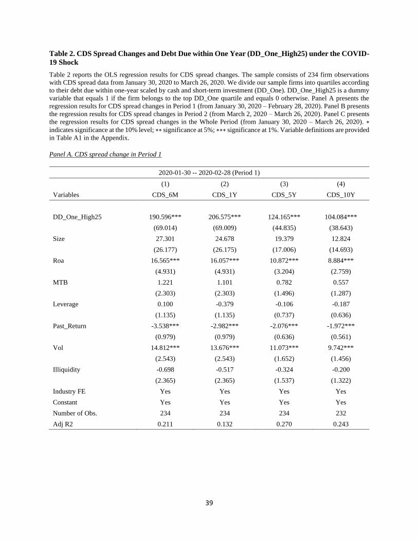
39
Table 2. CDS Spread Changes and Debt Due within One Year (DD_One_High25) under the COVID-
19 Shock
Table 2 reports the OLS regression results for CDS spread changes. The sample consists of 234 firm observations
with CDS spread data from January 30, 2020 to March 26, 2020. We divide our sample firms into quartiles according
to their debt due within one-year scaled by cash and short-term investment (DD_One). DD_One_High25 is a dummy
variable that equals 1 if the firm belongs to the top DD_One quartile and equals 0 otherwise. Panel A presents the
regression results for CDS spread changes in Period 1 (from January 30, 2020 – February 28, 2020). Panel B presents
the regression results for CDS spread changes in Period 2 (from March 2, 2020 – March 26, 2020). Panel C presents
the regression results for CDS spread changes in the Whole Period (from January 30, 2020 – March 26, 2020). ∗
indicates significance at the 10% level; ∗∗ significance at 5%; ∗∗∗ significance at 1%. Variable definitions are provided
in Table A1 in the Appendix.
Panel A. CDS spread change in Period 1
2020-01-30 -- 2020-02-28 (Period 1)
(1) (2) (3) (4)
Variables CDS_6M CDS_1Y CDS_5Y CDS_10Y
DD_One_High25 190.596*** 206.575*** 124.165*** 104.084***
(69.014) (69.009) (44.835) (38.643)
Size 27.301 24.678 19.379 12.824
(26.177) (26.175) (17.006) (14.693)
Roa 16.565*** 16.057*** 10.872*** 8.884***
(4.931) (4.931) (3.204) (2.759)
MTB 1.221 1.101 0.782 0.557
(2.303) (2.303) (1.496) (1.287)
Leverage 0.100 -0.379 -0.106 -0.187
(1.135) (1.135) (0.737) (0.636)
Past_Return -3.538*** -2.982*** -2.076*** -1.972***
(0.979) (0.979) (0.636) (0.561)
Vol 14.812*** 13.676*** 11.073*** 9.742***
(2.543) (2.543) (1.652) (1.456)
Illiquidity -0.698 -0.517 -0.324 -0.200
(2.365) (2.365) (1.537) (1.322)
Industry FE Yes Yes Yes Yes
Constant Yes Yes Yes Yes
Number of Obs. 234 234 234 232
Adj R2 0.211 0.132 0.270 0.243

40
Panel B. CDS spread change in Period 2
2020-03-02 -- 2020-03-26 (Period 2)
(1) (2) (3) (4)
Variables CDS_6M CDS_1Y CDS_5Y CDS_10Y
DD_One_High25 673.498*** 568.930*** 319.250*** 270.181***
(238.709) (211.349) (122.189) (103.619)
Size 94.141 87.151 47.331 33.984
(90.542) (80.164) (46.346) (39.202)
Roa 54.117*** 46.933*** 25.694*** 21.910***
(17.057) (15.102) (8.731) (7.495)
MTB 3.849 3.360 1.668 1.336
(7.967) (7.054) (4.078) (3.528)
Leverage 0.760 0.701 0.534 0.350
(3.926) (3.476) (2.009) (1.691)
Past_Return -11.106*** -10.082*** -5.138*** -4.720***
(3.386) (2.998) (1.733) (1.488)
Vol 53.058*** 49.138*** 29.010*** 24.711***
(8.797) (7.788) (4.503) (3.840)
Illiquidity -2.362 -2.177 -1.122 -0.878
(8.181) (7.243) (4.187) (3.511)
Industry FE Yes Yes Yes Yes
Constant Yes Yes Yes Yes
Number of Obs. 234 234 234 227
Adj R2 0.264 0.302 0.338 0.343
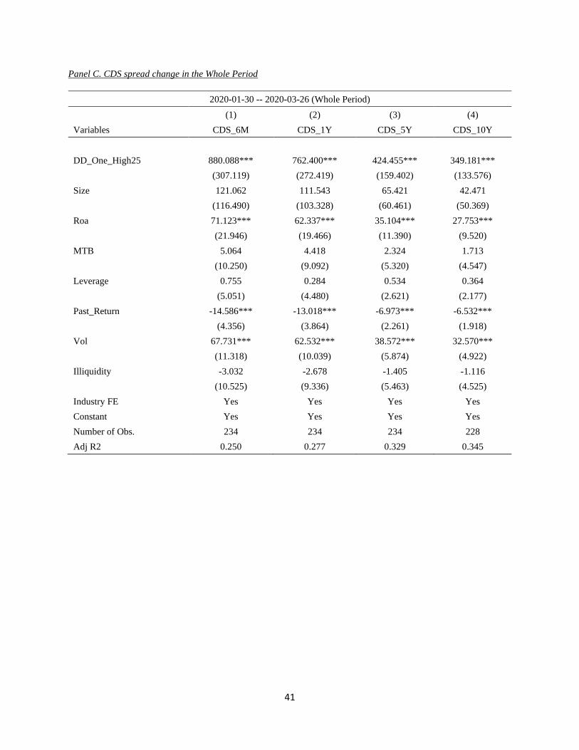
41
Panel C. CDS spread change in the Whole Period
2020-01-30 -- 2020-03-26 (Whole Period)
(1) (2) (3) (4)
Variables CDS_6M CDS_1Y CDS_5Y CDS_10Y
DD_One_High25 880.088*** 762.400*** 424.455*** 349.181***
(307.119) (272.419) (159.402) (133.576)
Size 121.062 111.543 65.421 42.471
(116.490) (103.328) (60.461) (50.369)
Roa 71.123*** 62.337*** 35.104*** 27.753***
(21.946) (19.466) (11.390) (9.520)
MTB 5.064 4.418 2.324 1.713
(10.250) (9.092) (5.320) (4.547)
Leverage 0.755 0.284 0.534 0.364
(5.051) (4.480) (2.621) (2.177)
Past_Return -14.586*** -13.018*** -6.973*** -6.532***
(4.356) (3.864) (2.261) (1.918)
Vol 67.731*** 62.532*** 38.572*** 32.570***
(11.318) (10.039) (5.874) (4.922)
Illiquidity -3.032 -2.678 -1.405 -1.116
(10.525) (9.336) (5.463) (4.525)
Industry FE Yes Yes Yes Yes
Constant Yes Yes Yes Yes
Number of Obs. 234 234 234 228
Adj R2 0.250 0.277 0.329 0.345
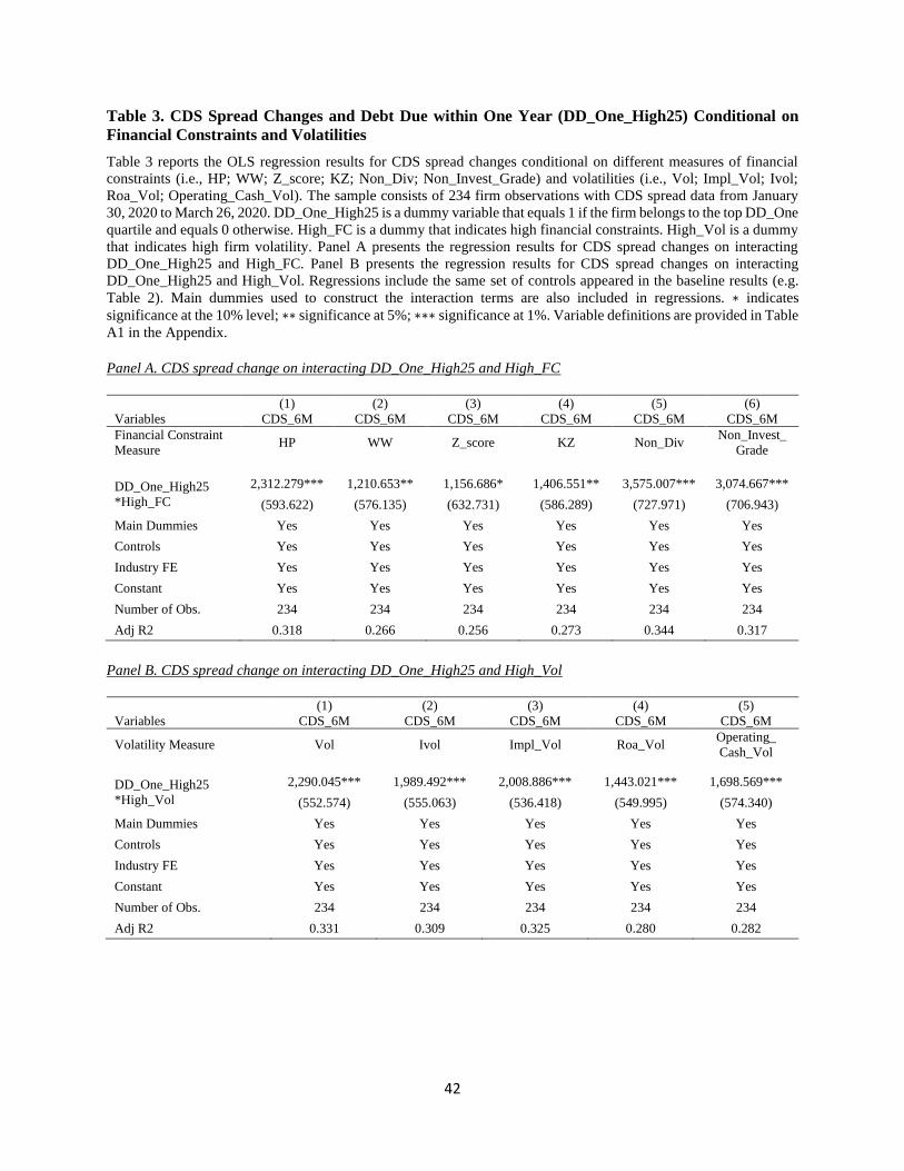
42
Table 3. CDS Spread Changes and Debt Due within One Year (DD_One_High25) Conditional on
Financial Constraints and Volatilities
Table 3 reports the OLS regression results for CDS spread changes conditional on different measures of financial
constraints (i.e., HP; WW; Z_score; KZ; Non_Div; Non_Invest_Grade) and volatilities (i.e., Vol; Impl_Vol; Ivol;
Roa_Vol; Operating_Cash_Vol). The sample consists of 234 firm observations with CDS spread data from January
30, 2020 to March 26, 2020. DD_One_High25 is a dummy variable that equals 1 if the firm belongs to the top DD_One
quartile and equals 0 otherwise. High_FC is a dummy that indicates high financial constraints. High_Vol is a dummy
that indicates high firm volatility. Panel A presents the regression results for CDS spread changes on interacting
DD_One_High25 and High_FC. Panel B presents the regression results for CDS spread changes on interacting
DD_One_High25 and High_Vol. Regressions include the same set of controls appeared in the baseline results (e.g.
Table 2). Main dummies used to construct the interaction terms are also included in regressions. ∗ indicates
significance at the 10% level; ∗∗ significance at 5%; ∗∗∗ significance at 1%. Variable definitions are provided in Table
A1 in the Appendix.
Panel A. CDS spread change on interacting DD_One_High25 and High_FC
(1) (2) (3) (4) (5) (6)
Variables CDS_6M CDS_6M CDS_6M CDS_6M CDS_6M CDS_6M
Financial Constraint
Measure HP WW Z_score KZ Non_Div
Non_Invest_
Grade
DD_One_High25
*High_FC
2,312.279*** 1,210.653** 1,156.686* 1,406.551** 3,575.007*** 3,074.667***
(593.622) (576.135) (632.731) (586.289) (727.971) (706.943)
Main Dummies Yes Yes Yes Yes Yes Yes
Controls Yes Yes Yes Yes Yes Yes
Industry FE Yes Yes Yes Yes Yes Yes
Constant Yes Yes Yes Yes Yes Yes
Number of Obs. 234 234 234 234 234 234
Adj R2 0.318 0.266 0.256 0.273 0.344 0.317
Panel B. CDS spread change on interacting DD_One_High25 and High_Vol
(1) (2) (3) (4) (5)
Variables CDS_6M CDS_6M CDS_6M CDS_6M CDS_6M
Volatility Measure Vol Ivol Impl_Vol Roa_Vol Operating_
Cash_Vol
DD_One_High25
*High_Vol
2,290.045*** 1,989.492*** 2,008.886*** 1,443.021*** 1,698.569***
(552.574) (555.063) (536.418) (549.995) (574.340)
Main Dummies Yes Yes Yes Yes Yes
Controls Yes Yes Yes Yes Yes
Industry FE Yes Yes Yes Yes Yes
Constant Yes Yes Yes Yes Yes
Number of Obs. 234 234 234 234 234
Adj R2 0.331 0.309 0.325 0.280 0.282

43
Table 4. Event Study on Stock Returns and Debt Due within One Year under the COVID-19 Shock
Table 4 reports event study results of the impact of COVID-19 on individual stock returns for U.S. listed firms. The
sample consists of 3,047 firm observations from January 30, 2020 to March 26, 2020. We divide our sample firms
into quartiles according to their debt due within one-year scaled by cash and short-term investment (DD_One)—group
1 has the lowest DD_One value and group 4 has the highest DD_One value. We report the mean of the buy and hold
abnormal returns (BHARs) and cumulative abnormal returns (CARs) for three periods: January 30, 2020 – February
28, 2020 (Period 1); March 2, 2020 – March 26, 2020 (Period 2); and January 30, 2020 – March 26, 2020 (Whole
Period). We calculate CARs using both the market model and the market-adjusted model. We use the S&P 500 stock
market index as the market portfolio. The market model estimation window is days (-150, -50) before the event date.
Panel A demonstrates results in BHARs. Panel B demonstrates results in CARs calculated using the market model.
Panel C demonstrates results in CARs calculated using the market-adjusted model. ∗ indicates significance at the 10%
level; ∗∗ significance at 5%; ∗∗∗ significance at 1%. Variable definitions are provided in Table A1 in the Appendix.
Panel A. BHARs
Group 1 Group 2 Group 3 Group 4 Total
2020-01-30 -- 2020-02-28 (Period 1) -0.634* 0.205 -1.975*** -1.924** -1.081**
(0.332) (0.432) (0.549) (0.752) (0.452)
2020-03-02 -- 2020-03-26 (Period 2) -11.464*** -7.255*** -12.126*** -14.618*** -11.365***
(2.089) (1.225) (1.472) (1.923) (1.487)
2020-01-30 -- 2020-03-26 (Whole Period) -10.516*** -6.041*** -11.926*** -14.079*** -10.639***
(2.013) (1.364) (1.553) (1.997) (1.551)
Number of Obs. 762 762 762 761 3,047
Panel B. CARs based on the market model
Group 1 Group 2 Group 3 Group 4 Total
2020-01-30 -- 2020-02-28 (Period 1) -1.505* 1.661* -0.998 -2.016*** -0.714
(0.859) (0.831) (0.705) (0.690) (0.739)
2020-03-02 -- 2020-03-26 (Period 2) -10.886*** -5.826*** -10.242*** -13.776*** -10.181***
(2.214) (1.328) (1.465) (1.754) (1.555)
2020-01-30 -- 2020-03-26 (Whole Period) -12.953*** -3.378 -11.681*** -16.769*** -11.194***
(3.115) (2.277) (2.170) (2.040) (2.401)
Number of Obs. 762 762 762 761 3,047
Panel C. CARs based on the market-adjusted model
Group 1 Group 2 Group 3 Group 4 Total
2020-01-30 -- 2020-02-28 (Period 1) -0.387 0.531 -2.030*** -1.931** -0.954*
(0.380) (0.496) (0.596) (0.819) (0.508)
2020-03-02 -- 2020-03-26 (Period 2) -9.466*** -6.064*** -10.756*** -13.221*** -9.876***
(1.765) (1.394) (1.465) (2.111) (1.478)
2020-01-30 -- 2020-03-26 (Whole Period) -9.657*** -5.393*** -12.435*** -14.848*** -10.582***
(2.075) (1.796) (1.951) (2.641) (1.912)
Number of Obs. 762 762 762 761 3,047
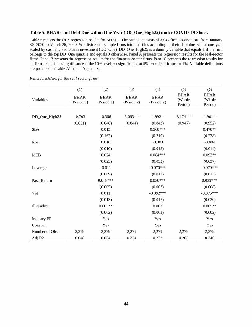
44
Table 5. BHARs and Debt Due within One Year (DD_One_High25) under COVID-19 Shock
Table 5 reports the OLS regression results for BHARs. The sample consists of 3,047 firm observations from January
30, 2020 to March 26, 2020. We divide our sample firms into quartiles according to their debt due within one-year
scaled by cash and short-term investment (DD_One). DD_One_High25 is a dummy variable that equals 1 if the firm
belongs to the top DD_One quartile and equals 0 otherwise. Panel A presents the regression results for the real-sector
firms. Panel B presents the regression results for the financial-sector firms. Panel C presents the regression results for
all firms. ∗ indicates significance at the 10% level; ∗∗ significance at 5%; ∗∗∗ significance at 1%. Variable definitions
are provided in Table A1 in the Appendix.
Panel A. BHARs for the real-sector firms
(1) (2) (3) (4) (5) (6)
Variables BHAR
(Period 1)
BHAR
(Period 1)
BHAR
(Period 2)
BHAR
(Period 2)
BHAR
(Whole
Period)
BHAR
(Whole
Period)
DD_One_High25 -0.703 -0.356 -3.063*** -1.992** -3.174*** -1.961**
(0.631) (0.648) (0.844) (0.842) (0.947) (0.952)
Size 0.015 0.568*** 0.478**
(0.162) (0.210) (0.238)
Roa 0.010 -0.003 -0.004
(0.010) (0.013) (0.014)
MTB 0.024 0.084*** 0.092**
(0.025) (0.032) (0.037)
Leverage -0.011 -0.070*** -0.070***
(0.009) (0.011) (0.013)
Past_Return 0.018*** 0.030*** 0.039***
(0.005) (0.007) (0.008)
Vol 0.011 -0.092*** -0.075***
(0.013) (0.017) (0.020)
Illiquidity 0.003** 0.003 0.005**
(0.002) (0.002) (0.002)
Industry FE Yes Yes Yes
Constant Yes Yes Yes
Number of Obs. 2,279 2,279 2,279 2,279 2,279 2,279
Adj R2 0.048 0.054 0.224 0.272 0.203 0.240

45
Panel B. BHARs for the financial firms
(1) (2) (3) (4) (5) (6)
Variables BHAR
(Period 1)
BHAR
(Period 1)
BHAR
(Period 2)
BHAR
(Period 2)
BHAR
(Whole
Period)
BHAR
(Whole
Period)
DD_One_High25 0.833 0.517 -1.271 0.462 -0.343 0.995
(0.615) (0.607) (1.276) (1.276) (1.322) (1.327)
Size -0.545*** -0.541* -0.864**
(0.154) (0.323) (0.336)
Roa 0.048*** 0.055 0.086**
(0.017) (0.035) (0.036)
MTB -0.048 0.020 -0.028
(0.037) (0.077) (0.080)
Leverage 0.038*** -0.110*** -0.071***
(0.010) (0.022) (0.023)
Past_Return 0.001 0.067*** 0.063***
(0.010) (0.022) (0.023)
Vol -0.060** 0.013 -0.008
(0.024) (0.050) (0.052)
Illiquidity 0.005*** 0.001 0.004*
(0.001) (0.003) (0.003)
Industry FE Yes Yes Yes
Constant Yes Yes Yes
Number of Obs. 768 768 768 768 768 768
Adj R2 0.005 0.076 0.118 0.161 0.099 0.136

46
Panel C. BHARs for all firms
(1) (2) (3) (4) (5) (6)
Variables BHAR
(Period 1)
BHAR
(Period 1)
BHAR
(Period 2)
BHAR
(Period 2)
BHAR
(Whole
Period)
BHAR
(Whole
Period)
DD_One_High25 -0.305 -0.075 -2.599*** -1.348* -2.440*** -1.152
(0.495) (0.506) (0.708) (0.707) (0.781) (0.786)
Size -0.132 0.227 0.075
(0.125) (0.175) (0.194)
Roa 0.016* 0.009 0.011
(0.008) (0.012) (0.013)
MTB 0.014 0.087*** 0.087***
(0.021) (0.029) (0.033)
Leverage -0.001 -0.077*** -0.069***
(0.007) (0.010) (0.011)
Past_Return 0.018*** 0.032*** 0.041***
(0.005) (0.007) (0.007)
Vol 0.001 -0.089*** -0.078***
(0.012) (0.016) (0.018)
Illiquidity 0.004*** 0.003 0.005***
(0.001) (0.002) (0.002)
Industry FE Yes Yes Yes
Constant Yes Yes Yes
Number of Obs. 3,047 3,047 3,047 3,047 3,047 3,047
Adj R2 0.047 0.056 0.208 0.251 0.188 0.222
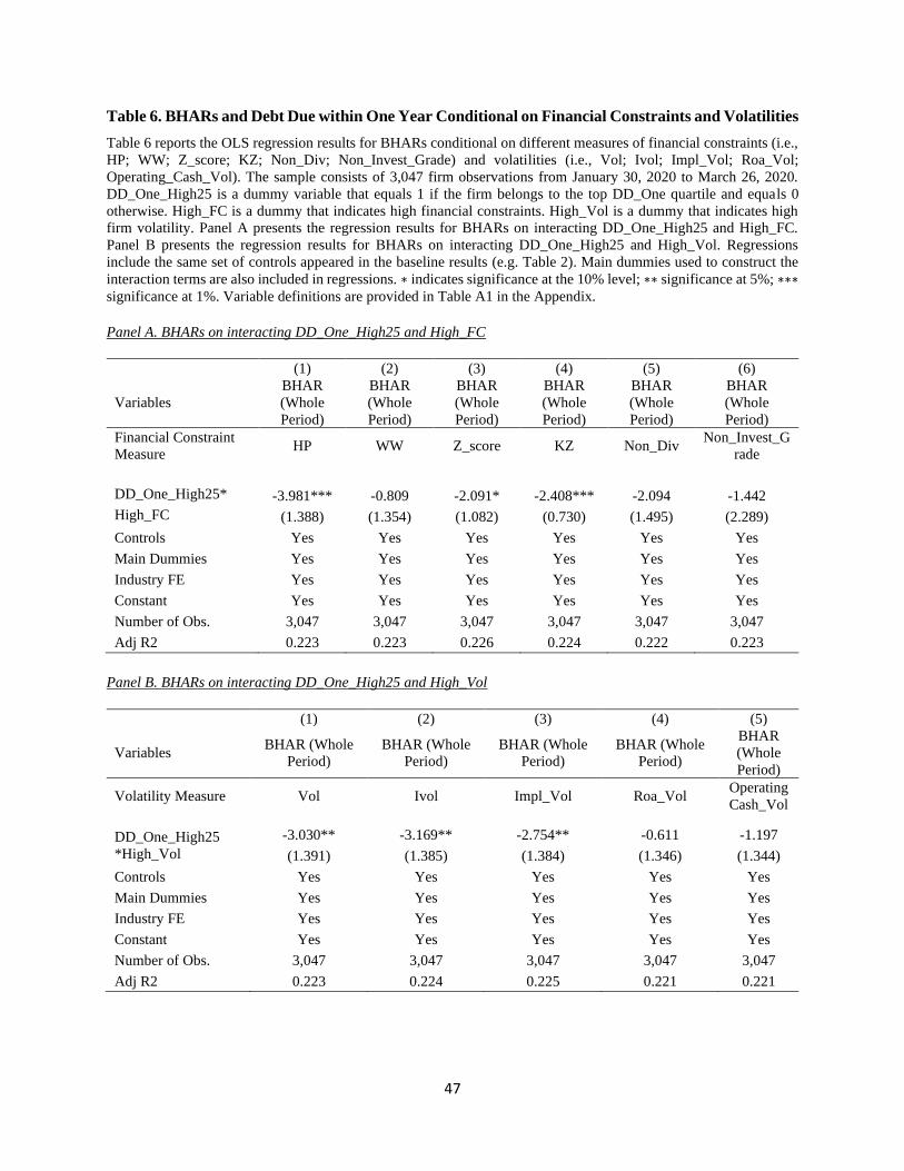
47
Table 6. BHARs and Debt Due within One Year Conditional on Financial Constraints and Volatilities
Table 6 reports the OLS regression results for BHARs conditional on different measures of financial constraints (i.e.,
HP; WW; Z_score; KZ; Non_Div; Non_Invest_Grade) and volatilities (i.e., Vol; Ivol; Impl_Vol; Roa_Vol;
Operating_Cash_Vol). The sample consists of 3,047 firm observations from January 30, 2020 to March 26, 2020.
DD_One_High25 is a dummy variable that equals 1 if the firm belongs to the top DD_One quartile and equals 0
otherwise. High_FC is a dummy that indicates high financial constraints. High_Vol is a dummy that indicates high
firm volatility. Panel A presents the regression results for BHARs on interacting DD_One_High25 and High_FC.
Panel B presents the regression results for BHARs on interacting DD_One_High25 and High_Vol. Regressions
include the same set of controls appeared in the baseline results (e.g. Table 2). Main dummies used to construct the
interaction terms are also included in regressions. ∗ indicates significance at the 10% level; ∗∗ significance at 5%; ∗∗∗
significance at 1%. Variable definitions are provided in Table A1 in the Appendix.
Panel A. BHARs on interacting DD_One_High25 and High_FC
(1) (2) (3) (4) (5) (6)
Variables
BHAR
(Whole
Period)
BHAR
(Whole
Period)
BHAR
(Whole
Period)
BHAR
(Whole
Period)
BHAR
(Whole
Period)
BHAR
(Whole
Period)
Financial Constraint
Measure HP WW Z_score KZ Non_Div
Non_Invest_G
rade
DD_One_High25* -3.981*** -0.809 -2.091* -2.408*** -2.094 -1.442
High_FC (1.388) (1.354) (1.082) (0.730) (1.495) (2.289)
Controls Yes Yes Yes Yes Yes Yes
Main Dummies Yes Yes Yes Yes Yes Yes
Industry FE Yes Yes Yes Yes Yes Yes
Constant Yes Yes Yes Yes Yes Yes
Number of Obs. 3,047 3,047 3,047 3,047 3,047 3,047
Adj R2 0.223 0.223 0.226 0.224 0.222 0.223
Panel B. BHARs on interacting DD_One_High25 and High_Vol
(1) (2) (3) (4) (5)
Variables BHAR (Whole
Period)
BHAR (Whole
Period)
BHAR (Whole
Period)
BHAR (Whole
Period)
BHAR
(Whole
Period)
Volatility Measure Vol Ivol Impl_Vol Roa_Vol Operating
Cash_Vol
DD_One_High25
*High_Vol
-3.030** -3.169** -2.754** -0.611 -1.197
(1.391) (1.385) (1.384) (1.346) (1.344)
Controls Yes Yes Yes Yes Yes
Main Dummies Yes Yes Yes Yes Yes
Industry FE Yes Yes Yes Yes Yes
Constant Yes Yes Yes Yes Yes
Number of Obs. 3,047 3,047 3,047 3,047 3,047
Adj R2 0.223 0.224 0.225 0.221 0.221

48
Table 7 CDS Spread Changes, BHARs and Debt Due within One Year by Months (Immediate Refinancing Needs vs Distant Refinancing
Needs) under COVID-19 Shock
Table 7 reports the OLS regression results for both CDS spread changes and BHARs under debt due within one-year measures with different maturity months. The
sample consists of 3,047 firm observations from January 30, 2020 to March 26, 2020. We merge and collect relevant debt maturity by months information in the
past 30 years from merged SDC New Debt Issuance and Dealscan Syndicated Loan databases. We divide our sample firms into quartiles according to either their
immediate debt due amount (debt due from March--June) or their distant debt due amount (debt due from July--December), both scaled by cash and short-term
investment, respectively. DD_One_High25 (March--June) is a dummy variable that equals 1 if the firm belongs to the top debt due from March to June scaled by
cash and short-term investment quartile and equals 0 otherwise. DD_One_High25 (July--December) is a dummy variable that equals 1 if the firm belongs to the
top debt due from July to December scaled by cash and short-term investment quartile and equals 0 otherwise. ∗ indicates significance at the 10% level; ∗∗
significance at 5%; ∗∗∗ significance at 1%. Variable definitions are provided in Table A1 in the Appendix.
The Influence of Debt Maturity Month (Immediate Refinancing Needs vs Distant Refinancing Needs)
CDS Spread Changes BHARs
Immediate Refinancing
(March-June)
Distant Refinancing
(July-December)
Immediate Refinancing
(March-June)
Distant Refinancing
(July-December)
VARIABLES CDS_6M CDS_1Y CDS_6M CDS_1Y BHAR
(Real Sector)
BHAR
(Financial
Sector)
BHAR
(Real Sector)
BHAR
(Financial
Sector)
DD_One_High25
(March -- June)
750.713** 666.566** -2.299** 0.918
(289.186) (256.226) (0.926) (1.314)
DD_One_High25
(July --December)
218.567 133.312 -1.770* 0.507
(314.426) (278.813) (0.927) (1.334)
Size 149.885 135.992 165.301 152.065 0.464* -0.860** 0.469** -0.856**
(115.857) (102.652) (118.174) (104.789) (0.237) (0.336) (0.237) (0.336)
Roa 81.350*** 71.453*** 69.800*** 61.112*** -0.003 0.086** -0.003 0.086**
(22.495) (19.932) (22.420) (19.881) (0.014) (0.036) (0.014) (0.036)
MTB 1.479 1.258 4.102 3.559 0.093** -0.028 0.093** -0.027
(10.331) (9.153) (10.468) (9.282) (0.037) (0.080) (0.037) (0.080)
Leverage 0.198 -0.237 1.650 1.145 -0.069*** -0.071*** -0.070*** -0.069***
(5.099) (4.518) (5.165) (4.580) (0.013) (0.023) (0.013) (0.023)
Past_Return -12.780*** -11.423*** -14.130*** -12.632*** 0.039*** 0.063*** 0.039*** 0.062***
(4.404) (3.902) (4.449) (3.945) (0.008) (0.023) (0.008) (0.023)
Vol 71.697*** 65.961*** 71.515*** 65.929*** -0.075*** -0.007 -0.076*** -0.008
(11.266) (9.982) (11.484) (10.183) (0.020) (0.052) (0.020) (0.052)
Illiquidity -6.097 -5.368 -3.579 -3.396 0.005** 0.004 0.005** 0.004*
(10.572) (9.367) (10.828) (9.602) (0.002) (0.003) (0.002) (0.003)
Industry FE Yes Yes Yes Yes Yes Yes Yes Yes
Constant Yes Yes Yes Yes Yes Yes Yes Yes
Observations 234 234 234 234 2,279 768 2,279 768
Adj R2 0.244 0.272 0.217 0.245 0.240 0.136 0.240 0.135
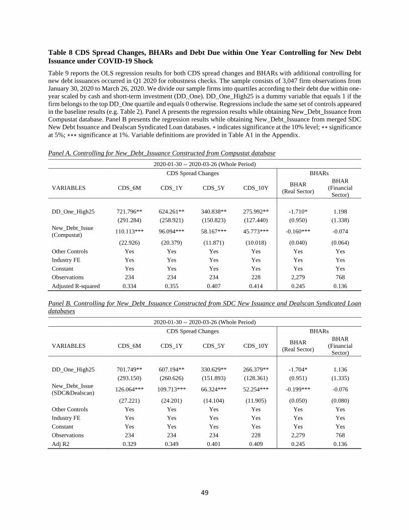
49
Table 8 CDS Spread Changes, BHARs and Debt Due within One Year Controlling for New Debt
Issuance under COVID-19 Shock
Table 9 reports the OLS regression results for both CDS spread changes and BHARs with additional controlling for
new debt issuances occurred in Q1 2020 for robustness checks. The sample consists of 3,047 firm observations from
January 30, 2020 to March 26, 2020. We divide our sample firms into quartiles according to their debt due within one-
year scaled by cash and short-term investment (DD_One). DD_One_High25 is a dummy variable that equals 1 if the
firm belongs to the top DD_One quartile and equals 0 otherwise. Regressions include the same set of controls appeared
in the baseline results (e.g. Table 2). Panel A presents the regression results while obtaining New_Debt_Issuance from
Compustat database. Panel B presents the regression results while obtaining New_Debt_Issuance from merged SDC
New Debt Issuance and Dealscan Syndicated Loan databases. ∗ indicates significance at the 10% level; ∗∗ significance
at 5%; ∗∗∗ significance at 1%. Variable definitions are provided in Table A1 in the Appendix.
Panel A. Controlling for New_Debt_Issuance Constructed from Compustat database
2020-01-30 -- 2020-03-26 (Whole Period)
CDS Spread Changes BHARs
VARIABLES CDS_6M CDS_1Y CDS_5Y CDS_10Y BHAR
(Real Sector)
BHAR
(Financial
Sector)
DD_One_High25 721.796** 624.261** 340.838** 275.992** -1.710* 1.198 (291.284) (258.921) (150.823) (127.440) (0.950) (1.338)
New_Debt_Issue
(Compustat) 110.113*** 96.094*** 58.167*** 45.773*** -0.160*** -0.074
(22.926) (20.379) (11.871) (10.018) (0.040) (0.064)
Other Controls Yes Yes Yes Yes Yes Yes
Industry FE Yes Yes Yes Yes Yes Yes
Constant Yes Yes Yes Yes Yes Yes
Observations 234 234 234 228 2,279 768
Adjusted R-squared 0.334 0.355 0.407 0.414 0.245 0.136
Panel B. Controlling for New_Debt_Issuance Constructed from SDC New Issuance and Dealscan Syndicated Loan
databases
2020-01-30 -- 2020-03-26 (Whole Period)
CDS Spread Changes BHARs
VARIABLES CDS_6M CDS_1Y CDS_5Y CDS_10Y BHAR
(Real Sector)
BHAR
(Financial
Sector)
DD_One_High25 701.749** 607.194** 330.629** 266.379** -1.704* 1.136 (293.150) (260.626) (151.893) (128.361) (0.951) (1.335)
New_Debt_Issue
(SDC&Dealscan) 126.064*** 109.713*** 66.324*** 52.254*** -0.199*** -0.076
(27.221) (24.201) (14.104) (11.905) (0.050) (0.080)
Other Controls Yes Yes Yes Yes Yes Yes
Industry FE Yes Yes Yes Yes Yes Yes
Constant Yes Yes Yes Yes Yes Yes
Observations 234 234 234 228 2,279 768
Adj R2 0.329 0.349 0.401 0.409 0.245 0.136

50
Table 9 CDS Spread Changes, BHARs and Alternative Debt Due within One Year Measures under
COVID-19 Shock
Table 8 reports the OLS regression results for both CDS spread changes and BHARs under two alternative debt due
within one-year measures for robustness checks. The sample consists of 3,047 firm observations from January 30,
2020 to March 26, 2020. We divide our sample firms into quartiles according to their debt due within one-year scaled
by either total debt amount (DD_One_Alternative 1) or total long-term debt amount (DD_One_Alternative 2),
respectively. DD_One_Alternative 1_High25 is a dummy variable that equals 1 if the firm belongs to the top debt due
within one-year scaled by total debt amount quartile and equals 0 otherwise. DD_One_Alternative 2_High25 is a
dummy variable that equals 1 if the firm belongs to the top debt due within one-year scaled by total long-term debt
amount quartile and equals 0 otherwise. Regressions include the same set of controls appeared in the baseline results
(e.g. Table 2). Panel A presents the regression results for the DD_One_Alternative 1 measures. Panel B presents the
regression results for the DD_One_Alternative 2 measures. ∗ indicates significance at the 10% level; ∗∗ significance
at 5%; ∗∗∗ significance at 1%. Variable definitions are provided in Table A1 in the Appendix.
Panel A. DD_One is defined as debt due within one-year divided by total debt amount
2020-01-30 -- 2020-03-26 (Whole Period)
CDS Spread
Changes BHARs
VARIABLES CDS_6M CDS_1Y CDS_5Y CDS_10Y BHAR (Real
Sector)
BHAR
(Financial
Sector)
DD_One_
Alternative 1_High25
815.402*** 706.693** 355.366** 260.421* -3.962** 2.835
(306.035) (271.414) (159.283) (133.445) (1.550) (1.904)
Controls Yes Yes Yes Yes Yes Yes
Industry FE Yes Yes Yes Yes Yes Yes
Constant Yes Yes Yes Yes Yes Yes
Observations 234 234 234 228 2,279 768
Adj R2 0.246 0.272 0.321 0.334 0.243 0.140
Panel B. DD_One is defined as debt due within one-year divided by long-term debt amount
2020-01-30 -- 2020-03-26 (Whole Period)
CDS Spread
Changes BHARs
VARIABLES CDS_6M CDS_1Y CDS_5Y CDS_10Y BHAR (Real
Sector)
BHAR
(Financial
Sector)
DD_One_
Alternative 2_High25
719.195** 617.337** 298.818* 214.691 -4.340*** 3.785*
(307.012) (272.304) (159.740) (133.648) (1.479) (1.810)
Controls Yes Yes Yes Yes Yes Yes
Industry FE Yes Yes Yes Yes Yes Yes
Constant Yes Yes Yes Yes Yes Yes
Observations 234 234 234 228 2,279 768
Adj R2 0.239 0.266 0.315 0.329 0.244 0.143

51
Table 10 CDS Spread Changes, BHARs and Debt Due within One Year before vs. around Government’s Relief Package
Table 10 reports the OLS regression results for both CDS spread changes and BHARs before vs. around government’s relief package. The two-trillion-dollar relief
package passed the U.S. Senate on March 25 and the House of Representatives on March 27. It was then immediately signed into law by President Trump on March
27. News about the rescue package sent the S&P 500 index up by 9.38% on March 24, which is the best day since October 28, 2008. The market has generally
been in an upward trend since then. The sample consists of 3,047 firm observations from January 30, 2020 to March 26, 2020. We divide our sample firms into
quartiles according to their debt due within one-year scaled by cash and short-term investment (DD_One). DD_One_High25 is a dummy variable that equals 1 if
the firm belongs to the top DD_One quartile and equals 0 otherwise. Regressions include the same set of controls appeared in the baseline results (e.g. Table 2). ∗
indicates significance at the 10% level; ∗∗ significance at 5%; ∗∗∗ significance at 1%. Variable definitions are provided in Table A1 in the Appendix.
The Influence of Government Relief Package (Pre-Relief Package vs. Post-Relief Package)
CDS Spread Changes BHARs
Before Relief
(Jan 30 to Mar 23, 2020)
Around Relief
(Mar 24 to Mar 26, 2020)
Before Relief
(Jan 30 to Mar 23, 2020)
Around Relief
(Mar 24 to Mar 26, 2020)
VARIABLES CDS_6M CDS_1Y CDS_6M CDS_1Y BHAR
(Real Sector)
BHAR
(Financial
Sector)
BHAR
(Real Sector)
BHAR
(Financial
Sector)
DD_One_High25 812.182*** 672.898*** -23.870 -20.571 -1.911** 1.485 0.566 -1.243
(288.431) (248.124) (22.922) (26.130) (0.936) (1.261) (0.737) (1.260)
Size 128.594 113.000 -5.225 -7.512 -0.142 -1.309*** 0.965*** 1.241***
(109.401) (94.113) (8.694) (9.911) (0.234) (0.319) (0.184) (0.319)
Roa 67.389*** 55.905*** -1.516 -1.607 0.011 0.074** -0.024** -0.004 (20.610) (17.730) (1.638) (1.867) (0.014) (0.034) (0.011) (0.034)
MTB 4.986 4.022 -0.228 -0.137 0.094*** -0.083 -0.043 0.103 (9.627) (8.281) (0.765) (0.872) (0.036) (0.076) (0.028) (0.076)
Leverage 0.293 0.673 -0.500 -0.624 -0.082*** -0.075*** 0.061*** 0.047** (4.743) (4.081) (0.377) (0.430) (0.013) (0.022) (0.010) (0.022)
Past_Return -13.343*** -11.515*** 0.162 0.284 0.021*** 0.032 0.027*** 0.025 (4.091) (3.520) (0.325) (0.371) (0.008) (0.021) (0.006) (0.021)
Vol 67.910*** 60.790*** -2.064** -3.154*** -0.063*** 0.018 -0.017 -0.067
(10.629) (9.144) (0.845) (0.963) (0.019) (0.049) (0.015) (0.049)
Illiquidity -2.778 -2.496 0.065 0.110 0.006*** 0.008*** -0.004* -0.009***
(9.885) (8.503) (0.786) (0.895) (0.002) (0.003) (0.002) (0.003)
Industry FE Yes Yes Yes Yes Yes Yes Yes Yes
Constant Yes Yes Yes Yes Yes Yes Yes Yes
Observations 234 234 234 234 2,279 768 2,279 768
Adj R2 0.283 0.309 -0.090 -0.030 0.222 0.175 0.135 0.145

52
Figure 1. CDS Spread Changes (6-Month) and Debt Due within One Year under the COVID-19
Shock
Figure 1 shows the cumulative CDS spread changes (6-month) for various groups. We divide our sample firms into
quartiles according to their debt due within one-year scaled by cash and short-term investments (DD_One)—group 1
has the lowest DD_One value and group 4 has the highest DD_One value).
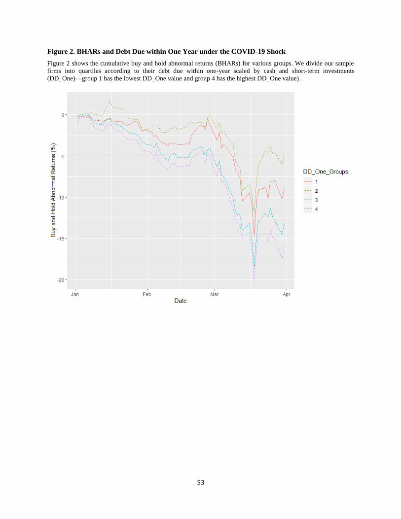
53
Figure 2. BHARs and Debt Due within One Year under the COVID-19 Shock
Figure 2 shows the cumulative buy and hold abnormal returns (BHARs) for various groups. We divide our sample
firms into quartiles according to their debt due within one-year scaled by cash and short-term investments
(DD_One)—group 1 has the lowest DD_One value and group 4 has the highest DD_One value).
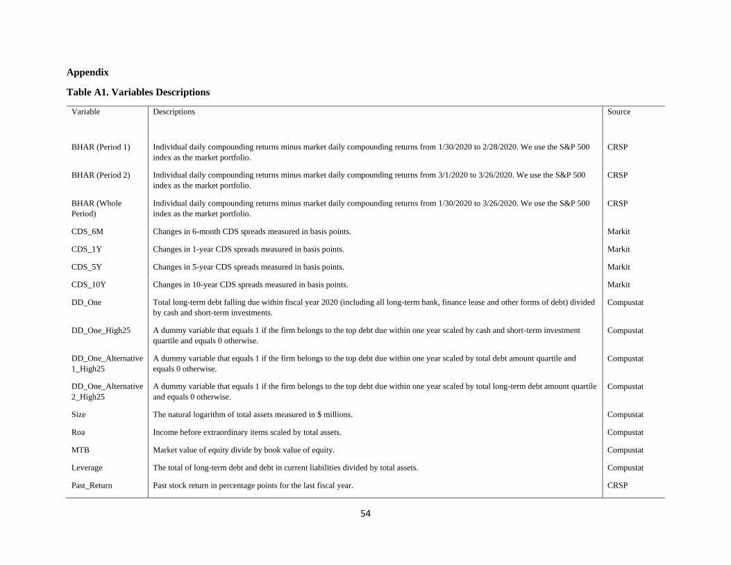
54
Appendix
Table A1. Variables Descriptions
Variable Descriptions Source
BHAR (Period 1) Individual daily compounding returns minus market daily compounding returns from 1/30/2020 to 2/28/2020. We use the S&P 500
index as the market portfolio.
CRSP
BHAR (Period 2) Individual daily compounding returns minus market daily compounding returns from 3/1/2020 to 3/26/2020. We use the S&P 500
index as the market portfolio.
CRSP
BHAR (Whole
Period)
Individual daily compounding returns minus market daily compounding returns from 1/30/2020 to 3/26/2020. We use the S&P 500
index as the market portfolio.
CRSP
CDS_6M Changes in 6-month CDS spreads measured in basis points. Markit
CDS_1Y Changes in 1-year CDS spreads measured in basis points. Markit
CDS_5Y Changes in 5-year CDS spreads measured in basis points. Markit
CDS_10Y Changes in 10-year CDS spreads measured in basis points. Markit
DD_One Total long-term debt falling due within fiscal year 2020 (including all long-term bank, finance lease and other forms of debt) divided
by cash and short-term investments.
Compustat
DD_One_High25 A dummy variable that equals 1 if the firm belongs to the top debt due within one year scaled by cash and short-term investment
quartile and equals 0 otherwise.
Compustat
DD_One_Alternative
1_High25
A dummy variable that equals 1 if the firm belongs to the top debt due within one year scaled by total debt amount quartile and
equals 0 otherwise.
Compustat
DD_One_Alternative
2_High25
A dummy variable that equals 1 if the firm belongs to the top debt due within one year scaled by total long-term debt amount quartile
and equals 0 otherwise.
Compustat
Size The natural logarithm of total assets measured in $ millions. Compustat
Roa Income before extraordinary items scaled by total assets. Compustat
MTB Market value of equity divide by book value of equity. Compustat
Leverage The total of long-term debt and debt in current liabilities divided by total assets. Compustat
Past_Return Past stock return in percentage points for the last fiscal year. CRSP
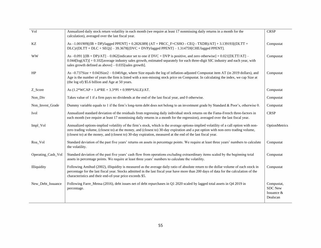
55
Vol Annualized daily stock return volatility in each month (we require at least 17 nonmissing daily returns in a month for the
calculation), averaged over the last fiscal year.
CRSP
KZ As –1.001909[(IB + DP)/lagged PPENT] + 0.2826389[ (AT + PRCC_F×CSHO - CEQ - TXDB)/AT] + 3.139193[(DLTT +
DLC)/(DLTT + DLC + SEQ)] – 39.3678[(DVC + DVP)/lagged PPENT] – 1.314759[CHE/lagged PPENT].
Compustat
WW As –0.091 [(IB + DP)/AT] – 0.062[indicator set to one if DVC + DVP is positive, and zero otherwise] + 0.021[DLTT/AT] –
0.044[log(AT)] + 0.102[average industry sales growth, estimated separately for each three-digit SIC industry and each year, with
sales growth defined as above] – 0.035[sales growth].
Compustat
HP As –0.737Size + 0.043Size2 – 0.040Age, where Size equals the log of inflation-adjusted Compustat item AT (in 2019 dollars), and
Age is the number of years the firm is listed with a non-missing stock price on Compustat. In calculating the index, we cap Size at
(the log of) $5.6 billion and Age at 50 years.
Compustat
Z_Score As (1.2*WCAP + 1.4*RE + 3.3*PI + 0.999*SALE)/AT. Compustat
Non_Div Takes value of 1 if a firm pays no dividends at the end of the last fiscal year, and 0 otherwise. Compustat
Non_Invest_Grade Dummy variable equals to 1 if the firm’s long-term debt does not belong to an investment grade by Standard & Poor’s, otherwise 0. Compustat
Ivol Annualized standard deviation of the residuals from regressing daily individual stock returns on the Fama-French three-factors in
each month (we require at least 17 nonmissing daily returns in a month for the regression), averaged over the last fiscal year.
CRSP
Impl_Vol Annualized options-implied volatility of the firm’s stock, which is the average options-implied volatility of a call option with non-
zero trading volume, (closest to) at the money, and (closest to) 30-day expiration and a put option with non-zero trading volume,
(closest to) at the money, and (closest to) 30-day expiration, measured at the end of the last fiscal year.
OptionMetrics
Roa_Vol Standard deviation of the past five years’ returns on assets in percentage points. We require at least three years’ numbers to calculate
the volatility.
Compustat
Operating_Cash_Vol Standard deviation of the past five years’ cash flow from operations excluding extraordinary items scaled by the beginning total
assets in percentage points. We require at least three years’ numbers to calculate the volatility.
Compustat
Illiquidity Following Amihud (2002), illiquidity is measured as the average daily ratio of absolute return to the dollar volume of each stock in
percentage for the last fiscal year. Stocks admitted in the last fiscal year have more than 200 days of data for the calculation of the
characteristics and their end-of-year price exceeds $5.
Compustat
New_Debt_Issuance Following Farre_Mensa (2016), debt issues net of debt repurchases in Q1 2020 scaled by lagged total assets in Q4 2019 in
percentage.
Compustat,
SDC New
Issuance &
Dealscan

56
Table A2. CDS Spread Changes and Debt Due within One Year (DD_One_Group4,
DD_One_Group3, and DD_One_Group2) under the COVID-19 Shock
Table A2 reports the OLS regression results for CDS spread changes. The sample consists of 234 firm observations
with CDS spread data from January 30, 2020 to March 26, 2020. We divide our sample firms into quartiles according
to their debt due within one-year scaled by cash and short-term investment (DD_One). DD_One_Group4,
DD_One_Group 3 and DD_One_Group2 are dummy variables that equal 1 if the firm belongs to the top, second to
the top, and third to the top, quartile according to the value of DD_One, respectively, and equal 0 otherwise. Panel A
presents the regression results for CDS spread changes in Period 1 (from January 30, 2020 – February 28, 2020). Panel
B presents the regression results for CDS spread changes in Period 2 (from March 2, 2020 – March 26, 2020). Panel
C presents the regression results for CDS spread changes in the Whole Period (from January 30, 2020 – March 26,
2020). ∗ indicates significance at the 10% level; ∗∗ significance at 5%; ∗∗∗ significance at 1%. Variable definitions
are provided in Table A1 in the Appendix.
Panel A. CDS spread change in Period 1
2020-01-30 -- 2020-02-28 (Period 1)
(1) (2) (3) (4)
Variables CDS_6M CDS_1Y CDS_5Y CDS_10Y
DD_One_Group4 223.574** 225.216** 142.974** 110.008**
(87.798) (88.059) (57.116) (49.482)
DD_One_Group3 69.865 38.253 38.736 18.687
(80.341) (80.580) (52.265) (45.670)
DD_One_Group2 -15.263 -5.895 -6.247 -15.435
(75.122) (75.345) (48.870) (42.431)
Size 25.756 23.888 18.572 12.203 (26.259) (26.337) (17.082) (14.773)
Roa 17.085*** 16.338*** 11.157*** 9.046*** (4.967) (4.981) (3.231) (2.788)
MTB 0.971 0.974 0.652 0.444 (2.321) (2.328) (1.510) (1.300)
Leverage 0.046 -0.415 -0.141 -0.171 (1.172) (1.175) (0.762) (0.657)
Past_Return -3.319*** -2.867*** -1.958*** -1.900*** (0.998) (1.001) (0.649) (0.573)
Vol 14.973*** 13.773*** 11.170*** 9.764*** (2.586) (2.594) (1.682) (1.480)
Illiquidity -0.700 -0.515 -0.323 -0.214
(2.371) (2.378) (1.542) (1.328)
Industry FE Yes Yes Yes Yes
Constant Yes Yes Yes Yes
Number of Obs. 234 234 234 232
Adj R2 0.209 0.124 0.266 0.238

57
Panel B. CDS spread change in Period 2
2020-03-02 -- 2020-03-26 (Period 2)
(1) (2) (3) (4)
Variables CDS_6M CDS_1Y CDS_5Y CDS_10Y
DD_One_Group4 739.926** 642.418** 349.903** 253.803*
(304.586) (269.593) (155.985) (133.611)
DD_One_Group3 135.928 143.489 58.765 -14.889
(278.718) (246.696) (142.737) (123.584)
DD_One_Group2 -20.139 -7.071 -0.546 -35.659
(260.611) (230.670) (133.464) (114.753)
Size 91.350 84.525 46.308 33.360
(91.096) (80.630) (46.652) (39.489)
Roa 55.115*** 47.967*** 26.114*** 21.849***
(17.230) (15.251) (8.824) (7.559)
MTB 3.401 2.945 1.508 1.233
(8.054) (7.128) (4.124) (3.565)
Leverage 0.630 0.524 0.455 0.464
(4.065) (3.598) (2.082) (1.749)
Past_Return -10.696*** -9.673*** -4.974*** -4.715***
(3.461) (3.063) (1.772) (1.528)
Vol 53.404*** 49.552*** 29.188*** 24.571***
(8.971) (7.940) (4.594) (3.898)
Illiquidity -2.355 -2.154 -1.110 -0.918
(8.225) (7.280) (4.212) (3.533)
Industry FE Yes Yes Yes Yes
Constant Yes Yes Yes Yes
Number of Obs. 234 234 234 227
Adj R2 0.257 0.296 0.331 0.336
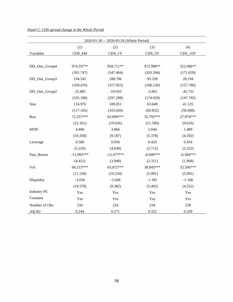
58
Panel C. CDS spread change in the Whole Period
2020-01-30 -- 2020-03-26 (Whole Period)
(1) (2) (3) (4)
Variables CDS_6M CDS_1Y CDS_5Y CDS_10Y
DD_One_Group4 974.197** 858.711** 472.998** 352.946**
(391.747) (347.464) (203.394) (171.659)
DD_One_Group3 194.541 188.796 95.339 28.194
(358.476) (317.953) (186.120) (157.780)
DD_One_Group2 -32.881 -10.910 -5.901 -45.731
(335.188) (297.298) (174.029) (147.705)
Size 116.976 108.051 63.649 41.125
(117.165) (103.920) (60.832) (50.698)
Roa 72.557*** 63.699*** 35.792*** 27.974***
(22.161) (19.656) (11.506) (9.616)
MTB 4.406 3.866 2.044 1.489
(10.358) (9.187) (5.378) (4.592)
Leverage 0.580 0.056 0.420 0.454
(5.229) (4.638) (2.715) (2.252)
Past_Return -13.993*** -12.477*** -6.699*** -6.384***
(4.451) (3.948) (2.311) (1.968)
Vol 68.213*** 63.072*** 38.843*** 32.506***
(11.538) (10.234) (5.991) (5.001)
Illiquidity -3.026 -2.649 -1.391 -1.160
(10.578) (9.382) (5.492) (4.552)
Industry FE Yes Yes Yes Yes
Constant Yes Yes Yes Yes
Number of Obs. 234 234 234 228
Adj R2 0.244 0.271 0.322 0.339

59
Table A3. CDS Spread Changes and Debt Due within One Year (DD_One_Group4,
DD_One_Group3 and DD_One_Group2) Conditional on Financial Constraints and Volatilities
Table A3 reports the OLS regression results for CDS spread changes conditional on different measures of financial
constraints (i.e., HP; WW; Z_score; KZ; Non_Div; Non_Invest_Grade) and volatilities (i.e., Vol; Impl_Vol; Ivol;
Roa_Vol; Operating_Cash_Vol). The sample consists of 234 firm observations with CDS spread data from January
30, 2020 to March 26, 2020. High_FC is a dummy that indicates high financial constraints. High_Vol is a dummy that
indicates high firm volatility. Panel A presents the regression results for CDS spread changes on interacting
DD_One_Group4, DD_One_Group3, DD_One_Group2 and High_FC. Panel B presents the regression results for
CDS spread changes on interacting DD_One_Group4, DD_One_Group3, DD_One_Group2 and High_Vol.
Regressions include the same set of controls appeared in the baseline results (e.g. Table 2). Main dummies used to
construct the interaction terms are also included. ∗ indicates significance at the 10% level; ∗∗ significance at 5%; ∗∗∗
significance at 1%. Variable definitions are provided in Table A1 in the Appendix.
Panel A. CDS spread change on interacting DD_One_Group4, DD_One_Group3, DD_One_Group2 and High_FC
(1) (2) (3) (4) (5) (6)
Variables CDS_6M CDS_6M CDS_6M CDS_6M CDS_6M CDS_6M
Financial Constraint
Measure HP WW Z_score KZ Non_Div
Non_Invest_
Grade
DD_One_Group4*
High_FC
2,068.376*** 1,007.194 1,099.353 905.904 3,733.480*** 2,720.286***
(688.516) (691.899) (775.551) (694.430) (857.373) (913.142)
DD_One_Group3*
High_FC
-561.427 -371.384 -75.908 -843.476 467.741 -381.958
(613.152) (636.804) (685.165) (635.372) (997.822) (871.202)
DD_One_Group2*
High_FC
-143.022 -189.731 -213.222 -664.589 214.094 -701.354
(614.737) (637.124) (668.428) (638.562) (897.595) (954.299)
Controls Yes Yes Yes Yes Yes Yes
Main Dummies Yes Yes Yes Yes Yes Yes
Industry FE Yes Yes Yes Yes Yes Yes
Constant Yes Yes Yes Yes Yes Yes
Number of Obs. 234 234 234 234 234 234
Adj R2 0.307 0.252 0.242 0.267 0.330 0.306
Panel B. CDS spread change on interacting DD_One_Group4, DD_One_Group3, DD_One_Group2 and High_Vol
(1) (2) (3) (4) (5)
Variables CDS_6M CDS_6M CDS_6M CDS_6M CDS_6M
Volatility Measure Vol Ivol Impl_Vol Roa_Vol Operating_
Cash_Vol
DD_One_Group4*High_Vol 2,368.742*** 2,063.652*** 1,954.251*** 1,509.180** 1,699.692** (654.293) (660.761) (638.541) (668.365) (696.629)
DD_One_Group3*High_Vol 209.555 138.883 -100.519 156.216 -138.855 (600.834) (599.730) (600.247) (648.313) (641.123)
DD_One_Group2*High_Vol 52.464 103.398 -32.928 17.812 147.703 (608.289) (601.792) (609.462) (654.078) (636.076)
Controls Yes Yes Yes Yes Yes
Main Dummies Yes Yes Yes Yes Yes
Industry FE Yes Yes Yes Yes Yes
Constant Yes Yes Yes Yes Yes
Number of Obs. 234 234 234 234 234
Adj R2 0.317 0.295 0.311 0.267 0.269

60
Table A4. BHARs and Debt Due within One Year (DD_One_Group4, DD_One_Group3, and
DD_One_Group2) under COVID-19 Shock
Table A4 reports the OLS regression results for BHARs. The sample consists of 3,047 firm observations from January
30, 2020 to March 26, 2020. We divide our sample firms into quartiles according to their debt due within one-year
scaled by cash and short-term investment (DD_One). DD_One_Group4, DD_One_Group 3 and DD_One_Group2 are
dummy variables that equal 1 if the firm belongs to the top, second to the top, and third to the top, quartile according
to the value of DD_One, respectively, and equal 0 otherwise. Panel A presents the regression results for the real-sector
firms. Panel B presents the regression results for the financial-sector firms. Panel C presents the regression results for
all firms. ∗ indicates significance at the 10% level; ∗∗ significance at 5%; ∗∗∗ significance at 1%. Variable definitions
are provided in Table A1 in the Appendix.
Panel A. BHARs for the real-sector firms
(1) (2) (3) (4) (5) (6)
Variables BHAR
(Period 1)
BHAR
(Period 1)
BHAR
(Period 2)
BHAR
(Period 2)
BHAR
(Whole
Period)
BHAR
(Whole
Period)
DD_One_Group4 -0.580 -0.301 -3.216*** -2.752** -3.237*** -2.525*
(0.832) (0.881) (1.110) (1.143) (1.244) (1.291)
DD_One_Group3 -0.705 -0.655 -1.634 -2.190** -1.977* -2.308*
(0.775) (0.813) (1.035) (1.055) (1.159) (1.192)
DD_One_Group2 1.446* 1.381* 1.947* 1.370 2.748** 2.261**
(0.772) (0.780) (1.030) (1.012) (1.154) (1.143)
Size 0.062 0.685*** 0.611** (0.165) (0.214) (0.241)
Roa 0.010 -0.003 -0.004 (0.010) (0.013) (0.014)
MTB 0.021 0.078** 0.085** (0.025) (0.032) (0.036)
Leverage -0.009 -0.064*** -0.063*** (0.009) (0.012) (0.013)
Past_Return 0.018*** 0.029*** 0.038*** (0.005) (0.007) (0.008)
Vol 0.011 -0.091*** -0.075*** (0.013) (0.017) (0.020)
Illiquidity 0.003** 0.003 0.005**
(0.002) (0.002) (0.002)
Industry FE Yes Yes Yes
Constant Yes Yes Yes
Number of Obs. 2,279 2,279 2,279 2,279 2,279 2,279
Adj R2 0.052 0.057 0.229 0.276 0.210 0.246
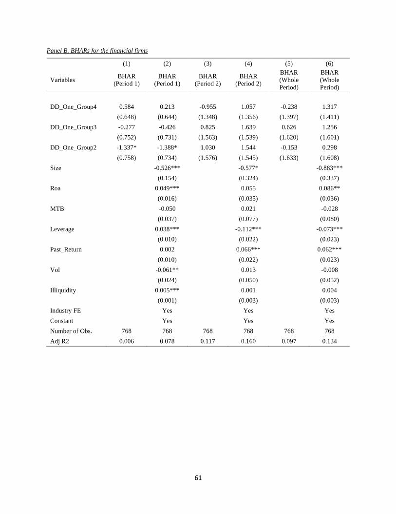
61
Panel B. BHARs for the financial firms
(1) (2) (3) (4) (5) (6)
Variables BHAR
(Period 1)
BHAR
(Period 1)
BHAR
(Period 2)
BHAR
(Period 2)
BHAR
(Whole
Period)
BHAR
(Whole
Period)
DD_One_Group4 0.584 0.213 -0.955 1.057 -0.238 1.317
(0.648) (0.644) (1.348) (1.356) (1.397) (1.411)
DD_One_Group3 -0.277 -0.426 0.825 1.639 0.626 1.256
(0.752) (0.731) (1.563) (1.539) (1.620) (1.601)
DD_One_Group2 -1.337* -1.388* 1.030 1.544 -0.153 0.298
(0.758) (0.734) (1.576) (1.545) (1.633) (1.608)
Size -0.526*** -0.577* -0.883***
(0.154) (0.324) (0.337)
Roa 0.049*** 0.055 0.086**
(0.016) (0.035) (0.036)
MTB -0.050 0.021 -0.028
(0.037) (0.077) (0.080)
Leverage 0.038*** -0.112*** -0.073***
(0.010) (0.022) (0.023)
Past_Return 0.002 0.066*** 0.062***
(0.010) (0.022) (0.023)
Vol -0.061** 0.013 -0.008
(0.024) (0.050) (0.052)
Illiquidity 0.005*** 0.001 0.004
(0.001) (0.003) (0.003)
Industry FE Yes Yes Yes
Constant Yes Yes Yes
Number of Obs. 768 768 768 768 768 768
Adj R2 0.006 0.078 0.117 0.160 0.097 0.134
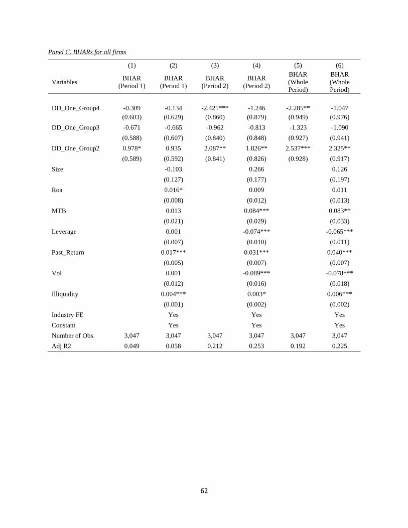
62
Panel C. BHARs for all firms
(1) (2) (3) (4) (5) (6)
Variables BHAR
(Period 1)
BHAR
(Period 1)
BHAR
(Period 2)
BHAR
(Period 2)
BHAR
(Whole
Period)
BHAR
(Whole
Period)
DD_One_Group4 -0.309 -0.134 -2.421*** -1.246 -2.285** -1.047
(0.603) (0.629) (0.860) (0.879) (0.949) (0.976)
DD_One_Group3 -0.671 -0.665 -0.962 -0.813 -1.323 -1.090
(0.588) (0.607) (0.840) (0.848) (0.927) (0.941)
DD_One_Group2 0.978* 0.935 2.087** 1.826** 2.537*** 2.325**
(0.589) (0.592) (0.841) (0.826) (0.928) (0.917)
Size -0.103 0.266 0.126
(0.127) (0.177) (0.197)
Roa 0.016* 0.009 0.011
(0.008) (0.012) (0.013)
MTB 0.013 0.084*** 0.083**
(0.021) (0.029) (0.033)
Leverage 0.001 -0.074*** -0.065***
(0.007) (0.010) (0.011)
Past_Return 0.017*** 0.031*** 0.040***
(0.005) (0.007) (0.007)
Vol 0.001 -0.089*** -0.078***
(0.012) (0.016) (0.018)
Illiquidity 0.004*** 0.003* 0.006***
(0.001) (0.002) (0.002)
Industry FE Yes Yes Yes
Constant Yes Yes Yes
Number of Obs. 3,047 3,047 3,047 3,047 3,047 3,047
Adj R2 0.049 0.058 0.212 0.253 0.192 0.225

63
Table A5. BHARs and Debt Due within One Year (DD_One_Group4, DD_One_Group3 and
DD_One_Group2) Conditional on Financial Constraints and Volatilities
Table A5 reports the OLS regression results for BHARs conditional on different measures of financial constraints (i.e.,
HP; WW; Z_score; KZ; Non_Div; Non_Invest_Grade) and volatilities (i.e., Vol; Impl_Vol; Ivol; Roa_Vol;
Operating_Cash_Vol). The sample consists of 234 firm observations with BHARs data from January 30, 2020 to
March 26, 2020. High_FC is a dummy that indicates high financial constraints. High_Vol is a dummy that indicates
high firm volatility. Panel A presents the regression results for BHARs on interacting DD_One_Group4,
DD_One_Group3, DD_One_Group2 and High_FC. Panel B presents the regression results for BHARs on interacting
DD_One_Group4, DD_One_Group3, DD_One_Group2 and High_Vol. Regressions include the same set of controls
appeared in the baseline results (e.g. Table 2). Main dummies used to construct the interaction terms are also included.
∗ indicates significance at the 10% level; ∗∗ significance at 5%; ∗∗∗ significance at 1%. Variable definitions are
provided in Table A1 in the Appendix.
Panel A. BHARs on interacting DD_One_Group4, DD_One_Group3, DD_One_Group2 and High_FC
(1) (2) (3) (4) (5) (6)
Variables
BHAR
(Whole
Period)
BHAR
(Whole
Period)
BHAR
(Whole
Period)
BHAR
(Whole
Period)
BHAR
(Whole
Period)
BHAR
(Whole
Period)
Financial Constraint
Measure HP WW Z_score KZ Non_Div
Non_Invest_Gr
ade
DD_One_Group4*
High_FC
-3.851*** -0.719 -3.383** -3.498*** -1.577 -3.165
(1.473) (1.363) (1.324) (1.344) (1.831) (3.418)
DD_One_Group3*
High_FC
-0.443 -0.449 -2.127 -2.932** -1.905 -3.156
(1.454) (1.308) (1.390) (1.258) (1.794) (3.158)
DD_One_Group2*
High_FC
0.437 0.309 -1.423 -1.290 2.748 -1.357
(1.478) (1.340) (1.363) (1.337) (1.796) (3.148)
Controls Yes Yes Yes Yes Yes Yes
Main Dummies Yes Yes Yes Yes Yes Yes
Industry FE Yes Yes Yes Yes Yes Yes
Constant Yes Yes Yes Yes Yes Yes
Number of Obs. 3,047 3,047 3,047 3,047 3,047 3,047
Adj R2 0.226 0.226 0.226 0.227 0.226 0.226
Panel B. BHARs on interacting DD_One_Group4, DD_One_Group3, DD_One_Group2 and High_Vol
(1) (2) (3) (4) (5)
Variables BHAR (Whole
Period)
BHAR (Whole
Period)
BHAR (Whole
Period)
BHAR (Whole
Period)
BHAR
(Whole
Period)
Volatility Measure Vol Ivol Impl_Vol Roa_Vol Operating_
Cash_Vol
DD_One_Group4*
High_Vol
-3.574** -3.836*** -2.610* -0.486 -1.120
(1.421) (1.417) (1.412) (1.355) (1.353)
DD_One_Group3*
High_Vol
-3.226** -2.804** -0.660 -0.017 -0.489
(1.320) (1.332) (1.322) (1.277) (1.276)
DD_One_Group2*
High_Vol
-0.483 -1.971 1.163 0.502 0.400
(1.385) (1.371) (1.330) (1.365) (1.362)
Controls Yes Yes Yes Yes Yes
Main Dummies Yes Yes Yes Yes Yes
Industry FE Yes Yes Yes Yes Yes
Constant Yes Yes Yes Yes Yes
Number of Obs. 3,047 3,047 3,047 3,047 3,047
Adj R2 0.227 0.228 0.229 0.224 0.224

64
Table A6 CDS Spread Changes, BHARs and Debt Due within One Year Controlling for Market
Leverage under the COVID-19 Shock
Table A6 reports the OLS regression results for both CDS spread changes and BHARs further controlling for market
leverage ratio for robustness checks. The sample consists of 3,047 firm observations from January 30, 2020 to March
26, 2020. We divide our sample firms into quartiles according to their debt due within one-year scaled by cash and
short-term investment (DD_One). DD_One_High25 is a dummy variable that equals 1 if the firm belongs to the top
DD_One quartile and equals 0 otherwise. We replace book leverage ratio in the baseline regression with market
leverage ratio for robustness check. ∗ indicates significance at the 10% level; ∗∗ significance at 5%; ∗∗∗ significance
at 1%. Variable definitions are provided in Table A1 in the Appendix.
2020-01-30 -- 2020-03-26 (Whole Period)
CDS Spread Changes BHARs
VARIABLES CDS_6M CDS_1Y CDS_5Y CDS_10Y
BHAR
(Real
Sector)
BHAR
(Financial
Sector)
DD_One_High25 771.547*** 654.699*** 365.201** 299.230** -2.840*** 0.264 (287.294) (251.213) (147.750) (123.705) (0.945) (1.300)
Size 151.586 139.253 82.761 56.797 0.242 -0.977*** (107.263) (93.792) (55.163) (45.992) (0.235) (0.333)
Roa 76.340*** 67.275*** 38.014*** 30.105*** -0.001 0.106*** (20.520) (17.943) (10.553) (8.812) (0.015) (0.036)
MTB 5.826 5.181 2.738 2.011 0.084** -0.015 (9.592) (8.387) (4.933) (4.213) (0.037) (0.079)
Market_Leverage 10.067*** 9.775*** 5.552*** 4.569*** -0.002 -0.090*** (2.021) (1.767) (1.040) (0.861) (0.007) (0.025)
Past_Return -10.896*** -9.453*** -4.933** -4.837*** 0.039*** 0.048** (4.139) (3.619) (2.129) (1.804) (0.008) (0.023)
Vol 70.726*** 65.190*** 40.289*** 33.890*** -0.088*** 0.018 (10.274) (8.984) (5.284) (4.415) (0.020) (0.052)
Illiquidity -4.429 -4.127 -2.152 -1.749 0.005** 0.004 (9.808) (8.576) (5.044) (4.175) (0.002) (0.003)
Industry FE Yes Yes Yes Yes Yes Yes
Constant Yes Yes Yes Yes Yes Yes
Observations 234 234 234 228 2,279 768
Adj R2 0.343 0.384 0.422 0.438 0.230 0.139

65
Table A7 CDS Spread Changes, BHARs and Debt Due within One Year Reacting to Interest Rate Reduction
Table A7 reports the OLS regression results for both CDS spread changes and BHARs reacting to the interest rate reduction by Federal Reserve announced on
March 15, 2020. The sample consists of 3,047 firm observations from January 30, 2020 to March 26, 2020. We investigate both the one-day (March 16) and two-
day (March 16 and March 17) market reactions to the interest rate reduction announcement made by Federal Reserve. We divide our sample firms into quartiles
according to their debt due within one-year scaled by cash and short-term investment (DD_One). DD_One_High25 is a dummy variable that equals 1 if the firm
belongs to the top DD_One quartile and equals 0 otherwise. ∗ indicates significance at the 10% level; ∗∗ significance at 5%; ∗∗∗ significance at 1%. Variable
definitions are provided in Table A1 in the Appendix.
The Influence of Cutting Interest Rate on March 15, 2020 by Federal Reserve
CDS Spread Changes BHARs
One-Day Reactions Two-Day Reactions One-Day Reactions Two-Day Reactions
VARIABLES CDS_6M CDS_1Y CDS_6M CDS_1Y BHAR
(Real Sector)
BHAR
(Financial
Sector)
BHAR
(Real Sector)
BHAR
(Financial
Sector)
DD_One_High25 18.811 54.097** 6.615 12.956 0.449 0.214 -0.264 1.007 (38.705) (26.742) (13.907) (14.806) (0.420) (0.635) (0.654) (0.980)
Size 12.137 13.612 3.193 6.058 -0.282*** -0.804*** -0.456*** -1.470*** (14.681) (10.143) (5.275) (5.616) (0.105) (0.161) (0.163) (0.248)
Roa 3.929 5.174*** 0.471 1.925* -0.004 0.012 0.003 0.021 (2.766) (1.911) (0.994) (1.058) (0.006) (0.017) (0.010) (0.027)
MTB 0.484 0.480 -0.017 0.100 -0.021 0.005 -0.006 -0.103* (1.292) (0.893) (0.464) (0.494) (0.016) (0.038) (0.025) (0.059)
Leverage 0.481 -0.002 0.229 0.209 -0.031*** -0.023** -0.039*** -0.067*** (0.637) (0.440) (0.229) (0.244) (0.006) (0.011) (0.009) (0.017)
Past_Return -1.055* -1.162*** 0.199 0.005 -0.017*** -0.015 -0.012** -0.002 (0.549) (0.379) (0.197) (0.210) (0.004) (0.011) (0.005) (0.017)
Vol 6.071*** 6.970*** 1.589*** 3.412*** -0.011 0.007 -0.014 -0.002 (1.426) (0.985) (0.512) (0.546) (0.009) (0.025) (0.014) (0.038)
Illiquidity -0.272 -0.149 -0.112 -0.172 0.005*** 0.005*** 0.003* -0.002 (1.326) (0.916) (0.477) (0.507) (0.001) (0.001) (0.002) (0.002)
Industry FE Yes Yes Yes Yes Yes Yes Yes Yes
Constant Yes Yes Yes Yes Yes Yes Yes Yes
Observations 234 234 234 234 2,279 768 2,279 768
Adj R2 0.059 0.312 0.002 0.292 0.184 0.196 0.214 0.285
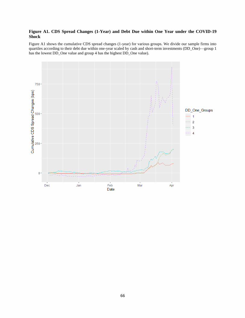
66
Figure A1. CDS Spread Changes (1-Year) and Debt Due within One Year under the COVID-19
Shock
Figure A1 shows the cumulative CDS spread changes (1-year) for various groups. We divide our sample firms into
quartiles according to their debt due within one-year scaled by cash and short-term investments (DD_One)—group 1
has the lowest DD_One value and group 4 has the highest DD_One value).

67
Figure A2. CDS Spread Changes (5-Year) and Debt Due within One Year under the COVID-19
Shock
Figure A2 shows the cumulative CDS spread changes (5-year) for various groups. We divide our sample firms into
quartiles according to their debt due within one-year scaled by cash and short-term investments (DD_One)—group 1
has the lowest DD_One value and group 4 has the highest DD_One value).
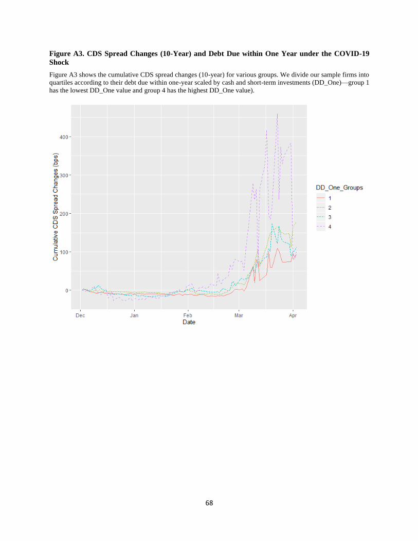
68
Figure A3. CDS Spread Changes (10-Year) and Debt Due within One Year under the COVID-19
Shock
Figure A3 shows the cumulative CDS spread changes (10-year) for various groups. We divide our sample firms into
quartiles according to their debt due within one-year scaled by cash and short-term investments (DD_One)—group 1
has the lowest DD_One value and group 4 has the highest DD_One value).