Debt Dynamics, Fiscal Deficit, and Stability in Government Borrowing in India: A Dynamic Panel Analysis

ADBI Working Paper Series

Debt Dynamics, Fiscal Deficit, and Stability in Government Borrowing in India: A Dynamic Panel Analysis

Panchanan Das

No. 557 March 2016

Asian Development Bank Institute

The Working Paper series is a continuation of the formerly named Discussion Paper series; the numbering of the papers continued without interruption or change. ADBI’s working papers reflect initial ideas on a topic and are posted online for discussion. ADBI encourages readers to post their comments on the main page for each working paper (given in the citation below). Some working papers may develop into other forms of publication.

Suggested citation:

Das, P. 2016. Debt Dynamics, Fiscal Deficit, and Stability in Government Borrowing in India: A Dynamic Panel Analysis. ADBI Working Paper 557. Tokyo: Asian Development Bank Institute. Available: http://www.adb.org/publications/debt-dynamics-fiscal-deficit-and-stability-government-borrowing-india-dynamic-panel/ Please contact the author for information about this paper.

Email: [email protected]

Panchanan Das is a professor at the University of Calcutta, India. The author is thankful to the discussants and participants at the conference, Central and Local Government Relations: Fiscal Sustainability, sponsored by the Asian Development Bank Institute and Zhongnan University of Economics and Law, held in Wuhan, People’s Republic of China, on 24–25 October 2015, for their valuable comments. The views expressed in this paper are the views of the author and do not necessarily reflect the views or policies of ADBI, ADB, its Board of Directors, or the governments they represent. ADBI does not guarantee the accuracy of the data included in this paper and accepts no responsibility for any consequences of their use. Terminology used may not necessarily be consistent with ADB official terms. Working papers are subject to formal revision and correction before they are finalized and considered published.

Asian Development Bank Institute Kasumigaseki Building 8F 3-2-5 Kasumigaseki, Chiyoda-ku Tokyo 100-6008, Japan Tel: +81-3-3593-5500 Fax: +81-3-3593-5571 URL: www.adbi.org E-mail: [email protected] © 2016 Asian Development Bank Institute

ADBI Working Paper 557 Das

Abstract Despite the initiatives of the Finance Commission of India, fiscal performance has been deteriorating and increasingly diverging across Indian states. Given that the state governments are endowed with expenditure autonomy, this paper investigates whether the composition of expenditure of the subnational governments has an impact on the degree of indebtedness. A panel analysis for the 17 non-special category states over 1980–2013 indicates that apart from the budget structure, the state-specific factors affecting fiscal performance plays an important role in government borrowing. Curiously enough, government borrowing is more responsive to revenue expenditure than capital outlay and has more growth-augmenting effect through revenue expenditure. JEL Classification: H72, H74, H77


Contents

1. Introduction ................................................................................................................ 3

2. Fiscal Capacity, Fiscal Health, and Government Borrowing ....................................... 4

3. Budget Deficit, Public Debt, and Economic Growth ................................................... 9

4. Empirical Analysis.................................................................................................... 10

5. Summary and Conclusions ...................................................................................... 15

References ......................................................................................................................... 17

Appendix ............................................................................................................................. 19


1. INTRODUCTION The debt and interest payments of the subnational governments have been increasing, although the rates have declined slowly in recent years in India. If fiscal deficits follow a course of a self-continuing rise in the debt to gross domestic product (GDP) ratio affecting adversely the growth rate, the fiscal policy would be inefficient creating a more serious debt problem. One popular way to stabilize the high debt to GDP ratio is to create primary surplus through restrictive fiscal policies at least temporarily by following the neoclassical solution. But, it is not an easy task for subnational governments in India to generate a primary surplus even in the short run, primarily because the subnational governments at the state level have limited power to raise tax revenues while they have to bear a lot of expenditure liabilities. Moreover, a benevolent government, both at the national and subnational levels, has some compulsions to provide different types of welfare benefits through the revenue account of the budget, creating more deficit. As the financial power and tax autonomy for the subnational governments are limited, control and reallocation of expenditure have been the primary source to adjust budget deficits. In this context, the expenditure side of the budget has a significant role in fiscal performance and government borrowing by influencing economic growth. The widening gap between revenues and expenditures in the states’ budgets has resulted in government borrowing. The interest rates applicable to the borrowing by the state governments are higher than the rate charged by the union government 1 in India. Borrowing by the government at the subnational level at higher interest rates has raised the debt servicing costs and worsened further their fiscal imbalance. Thus, fiscal deficits at the subnational level are more critical than those pertaining to the national government in India (Chelliah 2001). In effect, the fiscal federalism in India has been creating a vicious cycle of deficit and debt for many years, and the debt vulnerability as experienced recently in West Bengal, Punjab, and some other states in India is an outcome of it. Against this background, the main focus of this study is to look into whether the budget structure in terms of the allocation of expenditure by revenue and capital account has an influence on government borrowing and on economic growth in Indian states. The study investigates the current fiscal health of the state governments in terms of the major deficit and debt indicators. The analysis is based on panel data from 17 non-special category states2 in India from1980 to 2013. The effects of government expenditures of different types on the debt to GDP ratio and on economic growth have been estimated after controlling for fixed state specific effects. Potential endogeneity has been addressed by estimating the relationship with a one-way error component fixed effect model. The long-run debt–deficit behavior is analyzed within the framework developed by Domar (1944) on the basis of Keynes’ approach to public debt. Domar’s observation is a contrast to the neoclassical view that the primary deficit leads to an ever-growing public debt that inevitably leads to an increasing tax burden on the economy. One of the major hypotheses of Domar’s study is that if the GDP grows exponentially, the growth rate of debt converges to the growth rate of GDP and, thus, the ratio of debt to GDP will tend to a stationary state. It follows that higher proportional growth of

1 In India, the central government of India is officially referred to as the union government. 2 Special category states are given a higher share in the union government's resource allocation, due to

their severe topography, underdevelopment, and other social problems.

3


GDP reduces ultimately the ratio of debt to GDP. The higher the share of borrowing utilized in capital formation through the capital account, the greater will be the growth enhancing effect. Public investment in health, education, and research and development contributes to higher economic growth. The empirical results of this study indicate that state-specific unobserved factors mostly related to the budget management capabilities of the state governments and the motivation of the political parties in power in the states have had a decisive impact on the rise in government borrowing and on economic growth of the Indian states. The composition of government spending has had an effect on government debt as well as on the growth rate. Government borrowing has been increasing because of higher government spending on public consumption through the revenue account, not because of higher capital outlays. While the higher government spending in the revenue account by borrowing enhances GDP growth though the multiplier effect, it will increase debt. On the other hand, if government borrowing was used for capital formation, then growth potential of the economy would increase and the higher growth will ultimately reduce the share of public debt in GDP. The higher growth elasticity of revenue expenditure as observed in this study is mostly explained by the multiplier effect of Keynes’ type, but conflicting the way to fiscal adjustments on the sustainability of debt dynamics. The major contribution of the present study to the literature consists of analyzing in detail the regional variation of deficit structure and its impact on government borrowing and growth at the subnational level in the context of the fiscal reforms prescribed by the Finance Commission of India. The rest of the study is organized in the following way. Section 2 describes the regional variation in fiscal capacity, fiscal health, and the incidence of borrowing of the subnational governments within the federal fiscal structure as observed in India. Three major deficit indicators, namely, the revenue deficit, the primary deficit, and the gross fiscal deficit are used to analyze fiscal health of the state governments. Poor fiscal health is an indication of a high incidence of debt that varies significantly across the states. Section 3 presents different theoretical views on the relationship between budget deficit, public debt, and economic growth. Section 4 interprets the empirical results. The empirical analysis focuses on the impacts of the budget structure on the rise in debt burden of the state governments in India by decomposing total government expenditure in revenue and capital accounts. Section 5 concludes.

2. FISCAL CAPACITY, FISCAL HEALTH, AND GOVERNMENT BORROWING

Fiscal capacity of a state is measured conventionally by its own tax ratio. The variation of state’s own tax revenue as a percentage of its domestic product across the non-special category states as observed very recently is shown in Table 1. The tax ratio was the highest in Karnataka and the lowest in West Bengal in 2013–2014. The states exhibiting higher tax ratios during this fiscal year included Kerala, Tamil Nadu, Punjab, Goa, and Chhattisgarh. The tax ratio for most of the states remained roughly stable over the last three fiscal years. The higher tax ratio, however, is not necessarily an indicator of healthy fiscal position of an economy. As shown below, the fiscal performance in terms of deficit indicators of some states like Punjab and Kerala was not so sound despite their higher tax ratio. As the sources of revenues of the subnational governments in India are restricted, state governments depend highly on the national government for funds. The inter-governmental transfer, however, is a problem of political economy in a sense that the

4


design and implementation of a transfer system depends largely on political bargaining between the national and the subnational governments. It seems that the states with greater bargaining power manage to receive larger per capita transfer (Singh and Vasishtha 2004) and in the process horizontal imbalance remains a cause of concern along with the prominence of vertical imbalance. The transfer through the Finance Commission, although restricted to the non-plan side of the budget, plays an important role in correcting the horizontal imbalance.3 There has been a significant regional variation in the distribution of taxes collected by the union government as well as the grants provided by the central government (Table 1). The state’s share of central tax relative to the state’s domestic product was the highest, over 13%, in Bihar followed by Uttar Pradesh and Odisha4 in 2013–2014. The proportional share of central tax was the lowest at just about 1% in Haryana during the 2013–2014 fiscal year. The share of central tax as a percentage to state’s income was 4.4 in West Bengal in that period. Jharkhand got the highest central grant and Tamil Nadu got the lowest grant relative to states’ income in 2013–2014. The states displaying a higher ratio included Bihar, Chhattisgarh, and Odisha. In West Bengal, the ratio was moderate at 4.8.

Table 1: Own Tax, Share of Central Tax, and Central Grant by States in India Own Tax Revenue Share of Central Tax Central Grant 2011–

12 2012–

13 2013–

14 2011–

12 2012–

13 2013–

14 2011–

12 2012–

13 2013–

14 Andhra Pradesh 9.4 9.7 9.8 3.9 3.3 3.4 3.7 2.9 2.9 Bihar 6.0 6.3 7.0 16.4 13.4 13.3 9.0 8.4 7.9 Chhattisgarh 9.0 10.1 10.4 6.6 6.0 6.2 7.9 7.1 6.9 Goa 7.3 8.9 10.6 2.4 2.4 2.9 1.4 1.4 2.4 Gujarat 8.9 9.4 9.6 2.0 1.7 1.7 2.2 2.1 2.0 Haryana 7.8 8.1 8.5 1.3 1.1 1.1 2.0 2.6 2.6 Jharkhand 6.2 7.2 7.1 8.1 7.3 6.9 9.1 12.5 9.3 Karnataka 11.9 12.2 12.6 3.6 3.0 3.2 4.1 4.6 4.5 Kerala 9.8 10.7 11.7 2.9 2.4 2.6 2.7 2.4 2.5 Madhya Pradesh 10.3 9.3 8.7 8.6 7.1 6.4 7.2 5.6 5.2 Maharashtra 8.6 8.8 8.4 1.6 1.4 1.5 2.3 2.1 2.0 Odisha 7.9 7.5 7.8 9.1 7.0 7.5 9.4 7.0 6.7 Punjab 8.6 10.0 10.6 2.0 1.8 2.0 2.2 3.4 3.3 Rajasthan 7.4 7.7 7.8 5.4 4.6 4.9 4.2 3.1 3.2 Tamil Nadu 10.4 11.4 11.7 2.8 2.4 2.5 2.5 1.5 1.5 Uttar Pradesh 9.0 9.2 9.6 10.8 9.5 9.6 5.9 4.7 4.3 West Bengal 5.5 6.1 6.5 5.0 4.2 4.4 5.9 4.3 4.8 Note: Figures shown as a percentage to net state domestic product (NSDP) at current prices. Source: Author’s calculations with data from Reserve Bank of India. State Finances–A Study of Budgets, various years; Government of India, Central Statistics Office.

3 The Finance Commission decides on tax shares and makes grants. 4 In 2011, the Government of India approved the name change of the State of Orissa to Odisha. This

document reflects this change. However, when reference is made to policies that predate the name change, the formal name Orissa is retained.

5


In analyzing fiscal health at the subnational level, this paper focuses attention on revenue deficit, primary deficit, and gross fiscal deficit. The problems of fiscal deficit and public debt in an economy have been accumulated through a long-run process. The revenue deficits at the subnational level in India have persisted since the late 1980s, and the progressive deterioration in state finances started since the late 1990s. Deficits in the budget of most state governments recorded the highest levels with the lowest central transfers to states during the late 1990s and the beginning of the next decade. Growing revenue expenditure (particularly in the form of wages, salaries, and pensions), losses of state public sector enterprises, and declining transfers from the union government are mostly attributed to worsening finances of the states. In addition, states’ own tax revenue declined significantly partly because of different types of tax exemptions provided by the state governments to the private corporations in the process of competition to attract private capital in the wake of neoliberal reforms since the early 1990s. Revenue deficit increased at the highest rate in Bihar followed by Uttar Pradesh, Punjab, and West Bengal during the 1990s. Deficit in the revenue account, however, improved only in Goa over the 1980s and 1990s and in many states during 2000–2013, probably because of the initiation of fiscal reforms legislation. But in West Bengal, Kerala, and Gujarat the deficit deteriorated during this period and at a significantly higher rate in West Bengal. The poor performance of the states on revenue balance is due to the lack of revenue receipts to meet expenditure, including interest payments on past debt (Das forthcoming). The gross fiscal deficit also followed roughly the similar pattern. The deterioration in fiscal deficit during the 1990s was mainly because of a higher interest burden to the states. Table 2 displays a comparison of the deficit indicators (deficits relative to states’ income) among 17 non-special category states during the past 3 fiscal years. The most important indicator of fiscal health is revenue deficit. West Bengal was at the top in terms of revenue deficit relative to income in 2011–2012, but the revenue deficit declined significantly during the past 3 years and it ranked fourth in 2013–2014. Haryana registered the highest deficit in revenue account followed by Kerala and Punjab during the 2013–2014 fiscal year. Many states in India managed to create a surplus in the revenue balance recently because of the initiation of the fiscal responsibility legislation by following the recommendation of the Report of the Twelfth Finance Commission (GOI 2004). West Bengal’s poor performance (along with some other states) on revenue balance is due to the lack of revenue receipts to meet expenditure, including interest payments on past debt. The overall resource gap between receipt and expenditure, taking both the revenue and capital accounts together, is reflected in the fiscal deficit. Capital receipts cover receipts as capital in nature and capital expenditures comprise spending, usually met from the borrowed funds, to create capital assets. The gross fiscal deficit relative to states’ domestic product varied widely across the states with the highest deficit in Goa and the lowest in Maharashtra in 2013–2014. The gross fiscal deficit in West Bengal was significantly small during this period. Fiscal deficit less interest payments determines primary deficit, the extent of borrowing used by the government for current expenditures both in revenue and capital accounts. The remaining part of fiscal deficit is claimed by interest payments. The primary deficit on revenue account might show the true resource gap in the government budget. As the primary revenue balance (revenue deficit less interest payments) does not consider interest payment liabilities on past debts, a surplus in primary revenue account is required to reduce the overall revenue account deficit. All the non-special category states have experienced a surplus in the primary fiscal balance consistently during the

6


past three years, but unevenly across the states. West Bengal generated the highest surplus in primary balance while experiencing significant fiscal deficit.

Table 2: Major Deficit Indicators of State Governments Revenue Deficit Primary Deficit Gross Fiscal Deficit 2011–

12 2012–

13 2013–

14 2011–

12 2012–

13 2013–

14 2011–

12 2012–

13 2013–

14 Andhra Pradesh –0.53 –0.25 –0.13 –1.75 –1.73 –1.85 2.59 3.11 3.18 Bihar –2.17 0.28 –2.16 –1.91 –1.85 –1.84 2.66 6.33 2.78 Chhattisgarh –2.63 –1.57 –1.57 –0.96 –0.90 –0.78 0.65 3.33 3.33 Goa –0.79 1.03 0.56 –1.84 –1.97 –2.24 2.31 5.72 6.17 Gujarat –0.62 –0.67 –0.71 –2.09 –2.06 –2.07 2.13 3.11 3.15 Haryana 0.53 1.02 0.70 –1.44 –1.62 –1.77 2.62 2.61 2.56 Jharkhand –1.23 –3.26 –2.10 –1.94 –1.87 –1.62 1.66 2.44 2.72 Karnataka –1.15 –0.20 –0.12 –1.46 –1.45 –1.61 3.02 3.30 3.38 Kerala 2.95 1.10 0.65 –2.26 –2.24 –2.18 4.71 3.67 3.42 Madhya Pradesh –3.58 –1.93 –1.28 –1.89 –1.76 –1.58 2.08 3.14 3.01 Maharashtra 0.21 0.00 –0.01 –1.62 –1.59 –1.56 1.88 1.64 1.81 Odisha –3.17 –1.40 –0.81 –1.46 –2.13 –2.11 –0.35 1.32 2.53 Punjab 2.99 1.89 0.62 –2.72 –2.74 –2.67 3.73 3.73 3.29 Rajasthan –0.93 –0.19 –0.22 –2.18 –2.04 –1.98 1.01 2.73 2.83 Tamil Nadu –0.23 –0.07 –0.09 –1.44 –1.49 –1.66 2.86 2.96 2.97 Uttar Pradesh –1.14 –0.80 –1.25 –2.51 –2.35 –2.13 2.53 3.06 3.03 West Bengal 3.03 2.39 0.55 –3.27 –3.16 –3.04 3.68 3.75 2.11 Notes: Deficits are expressed as percentage to net state domestic product (NSDP) at current prices. The negative figures indicate surpluses. Source: Author’s calculations with data from Reserve Bank of India. State Finances–A Study of Budgets, various years; Government of India, Central Statistics Office.

As the states have limited capacity to generate revenue they are forced to borrow to meet their fiscal deficit, and higher fiscal deficit causes the higher incidence of indebtedness. A growing debt ratio implies that public expenditure is excessively devoted to unproductive spending primarily because of inefficient fiscal management of the state governments. Non-development expenditure on administrative services, salaries, pensions, and interest payments has grown considerably since the late 1980s in all states (Das forthcoming). As a result, revenue deficit relative to fiscal deficit increased disproportionately in every state during the 1990s. Many states, however, managed to control non-developmental expenditure through fiscal reforms during the later decades. Debt burden increased significantly in all states except Goa from 1980–1981 till the mid-2000s. Interest burden, measured by interest payment as a share of revenue receipts, increased everywhere in the country and at a higher rate during the 1990s. Average interest payments during 2000–2013 were the highest (over 37% of the revenue receipt) for West Bengal followed by Punjab exhibiting nearly one-fourth of its revenue receipt as interest for public borrowing during the same period. Rajasthan, Gujarat, and Kerala registered interest payments over 20% of their revenue receipt. Recently, the debt ratio declined, although slowly in most states in India (Table 3). In West Bengal, the debt burden was the highest among the non-special category states despite exhibiting moderate fiscal deficit in 2013–2014. If the fiscal deficit on revenue account gap for a state is relatively high, as in the case of West Bengal, the state is in a worse position. A very high debt ratio in West Bengal was strongly related to a high

7


revenue deficit relative to its fiscal deficit.5 Total debt stock in the state was over 36% of its net domestic product, registering the highest share among the non-special category states, and in Chhattisgarh it was lowest at below 13% during 2013–2014. Punjab ranked second followed by Uttar Pradesh in terms of debt liability during the same period. Since the late 1980s, subnational governments have been experiencing financial imbalance primarily because of growing non-development expenditure on administrative services, salaries, pensions, and interest payments. The interest payment liability of West Bengal was more than one fifth of its revenue receipt, far above the interest liability of other non-special category states, during this fiscal period. However, interest liability of the state declined over the past 3 fiscal years by following the fall in debt ratio. Interest payments have been one of the major components of revenue expenditure of states creating revenue deficits more vulnerable. A large debt ratio and corresponding larger proportion of interest payment is a cause of concern from the point of view of stability and sustainability of fiscal policy of the government of West Bengal.

Table 3: Debt Indicators of State Governments Total Outstanding Debt

Relative to NSDP (%) Interest Payment Relative to Revenue Receipt (%)

Revenue Deficit Relative to Fiscal Deficit (%)

2011–12

2012–13

2013–14

2011–12

2012–13

2013–14

2011–12

2012–13

2013–14

Andhra Pradesh 23.48 22.19 21.97 11.29 10.94 11.36 –0.20 –0.08 –0.04 Bihar 28.58 25.04 24.29 8.38 7.78 7.36 –0.82 0.04 –0.78 Chhattisgarh 13.82 13.02 12.96 4.60 3.99 3.34 –4.05 –0.47 –0.47 Goa 25.12 26.87 30.94 12.28 11.52 11.35 –0.34 0.18 0.09 Gujarat 27.58 25.89 25.25 17.36 16.15 15.93 –0.29 –0.21 –0.22 Haryana 16.95 18.23 18.64 13.09 13.51 14.39 0.20 0.39 0.27 Jharkhand 24.40 24.23 22.79 10.12 7.58 7.35 –0.74 –1.34 –0.77 Karnataka 22.97 22.94 20.88 8.68 8.07 8.67 –0.38 –0.06 –0.03 Kerala 30.86 30.65 30.79 16.55 14.61 13.21 0.63 0.30 0.19 Madhya Pradesh 27.29 24.32 21.30 8.47 8.29 8.19 –1.72 –0.61 –0.43 Maharashtra 21.66 20.54 20.24 14.43 13.28 13.53 0.11 0.00 –0.01 Odisha 26.60 22.71 20.36 6.41 9.89 9.77 9.05 –1.06 –0.32 Punjab 32.89 32.90 33.09 23.93 17.80 17.81 0.80 0.51 0.19 Rajasthan 27.55 25.95 25.25 13.84 12.41 11.97 –0.93 –0.07 –0.08 Tamil Nadu 18.99 19.45 19.51 10.41 10.02 10.99 –0.08 –0.02 –0.03 Uttar Pradesh 37.70 35.24 32.83 11.83 10.53 9.59 –0.45 –0.26 –0.41 West Bengal 40.16 38.35 36.66 27.06 24.72 22.05 0.82 0.64 0.26 NSDP = net state domestic product. Source: Author’s calculations with data from Reserve Bank of India. State Finances–A Study of Budgets, various years; Government of India, Central Statistics Office.

A sharp deterioration of financial health of the state governments during the past few decades has not only been because of state specific reasons, but also owing to the ever growing vertical imbalance (Report of the Tenth Finance Commission [GOI 1994]). As discussed above, the rate of deterioration of the fiscal health is not similar for all states in India. West Bengal among all non-special category states in India has been experiencing severe fiscal strain in terms of debt ratio as shown in Table 3. Rising

5 One can compare states’ fiscal performance on asset creation by comparing a ratio of revenue deficit relative to fiscal deficit, a part of fiscal deficit that does not transform to create government assets. If the fiscal deficit is caused by the revenue account gap, then it will be an idle deficit.

8


interest payments, inadequate recovery of user charges, rising expenditure on wages and salaries, and sluggishness in the central transfer of resources have been the major factors for the deterioration in the fiscal conditions of the Indian states (Reserve Bank of India 2002). While the states’ own revenue sources are not increasing fast enough to match their rising expenditure, central devolution and other assistance are not adequate to cover the gap. Revenue deficits have widened and borrowings are being increasingly used to meet revenue expenditure. Thus, there has been a marked deterioration in the fiscal health of all states in India since the early 1990s, reaching a peak in the mid-2000s in most states. While the fiscal health of the state governments has improved recently, the debt ratio and the interest payments are still alarming and the primary causes for growing debt ratio need to be analyzed. In this study I have estimated the relative contribution of revenue expenditure and capital expenditure to government borrowings in a framework of debt dynamics as suggested by Domar (1944) in the following section. The standard theory in public economics suggests that the erosion of fiscal viability will be more if the larger proportion of total borrowing is used for bridging the revenue deficit. Thus, the pattern of use of government borrowings is crucial as far as the sustainability of debt finance is concerned.

3. BUDGET DEFICIT, PUBLIC DEBT, AND ECONOMIC GROWTH

As discussed above, high fiscal deficit has left a legacy of huge public debt and growing interest payments. The escalating debt burden also has a serious implication for the fiscal imbalance of the states. In this context, an empirical estimation of the long-run relationship between debt and deficit has immense significance to examine whether the fiscal policies adopted by the state governments are sustainable. The sustainability of public debt ratio is an important issue as it can be regarded as an indicator of the efficiency of public finance. In the neoclassical model, budget deficits financed by borrowing have no expansionary effect on GDP. In this case interest rate rises crowd out the multiplier effect of private spending on GDP. The endogenous growth model, however, has favored government borrowing to finance the deficits if it is used in growth-enhancing sectors such as developmental expenditures on public infrastructure, education, and health (Barro 1990; Lucas 1988; Romer 1990). There was significant contribution to the analysis of debt sustainability by Diamond (1965) in a general equilibrium framework. He analyzed the effect of a positive stock of debt on long-term competitive equilibrium of an economy with neoclassical technology. Rankin and Roffia (2003) developed further a model of debt sustainability on the basis of this approach. The budget deficit in Keynes’ sense has a multiplier effect on aggregate demand that ultimately generates employment and income even when the deficit is financed by borrowing. The traditional Keynesian framework does not distinguish between alternative uses of the fiscal deficit as between government consumption or investment expenditure. It also fails to distinguish between alternative sources of financing the fiscal deficit through monetization or external or internal borrowing. Keynes, later on, put forward a detailed analysis of the budget by arguing that full employment may be ensured through the increase in capital expenditure keeping the revenue expenditure under control. But, capital expenditures should be efficient and carried out by following some economic principles (Keynes 1980). If public investment is capable to yield a positive return, the deficit will be controlled in the long run. Subsequent elaborations of

9


the Keynesian paradigm envisage that the multiplier-based expansion of output leads to a rise in the demand for money, and if money supply is fixed and the deficit is bond financed, interest rates would rise offsetting at least partially the multiplier effect. Keynesians argue that deficits may stimulate savings and investment even if interest rates rise, primarily because of the employment of unutilized resources. However, at full employment, deficits would lead to crowding out even in the Keynesian paradigm. On the basis of Keynes’ framework, Domar (1944) formulated the necessary conditions for fiscal sustainability. Domar’s model has been extended by Buiter (1985) and further developed by Blanchard et al. (1990). In this structure, the ratio of public debt to GDP will converge in the long run to its initial level to attain fiscal sustainability. Domar (1944) studied the relationship between budget deficits and the behavior of the ratio of the public debt to GDP over time. He argued that there need not be a tendency for debt to GDP ratio to grow indefinitely. According to him, if income grows at a constant percentage rate, the growth rate of debt will approach the growth rate of income and, therefore, the ratio of debt to GDP will tend to a stationary state. Thus, the problem of the debt ratio lies in the ability to make income grow rather than in attempting to reduce it without taking account of the effects of such a reduction on income. A higher growth of income can be achieved if sufficient amount of the expenditures is directed toward increasing the efficiency of production. This empirical study is based on an extended formulation of the theoretical framework developed in Domar (1944) with panel data from 17 non-special category states over 1980–2013. A similar type of model has been used by Rangarajan and Srivastava (2005) in studying India’s state finances. But, they considered the long-run constancy of the nominal growth rate and effective interest rate in their basic formulation of the model.

4. EMPIRICAL ANALYSIS This study addresses the question of how different types of government spending are responsible for the rise in debt at the subnational level in India. The study focuses on the impacts of the budget structure on the rise in debt burden of the state governments by decomposing total government expenditure in revenue and capital accounts. To examine the shape of debt–deficit relationship, I hypothesize that the states’ economic growth is more responsive to government spending on capital formation than to spending on public consumption. The more the growth rate is sensitive to capital expenditure, the lower the debt burden in terms of net interest payment will be (interest payment less return to capital). Thus, the larger the proportion of public debt toward capital outlay, the larger the growth rate will be, and debt will be sustainable. To test these hypotheses empirically I have used panel data for government borrowing, own tax ratio, and different components of government expenditures from 17 non-special category states over 34 years (1980–2013). The Reserve Bank of India publishes the data on state finances from budgets of the state governments. I have used this database in this study. The data on state government finances are based on the receipts and expenditure statements presented in the budget documents of the state governments over the years. Data on net state domestic products (NSDP) are collected from the National Accounts Division of the Central Statistical Office. States’ domestic products at constant (2004–2005) prices are used to find out economic growth and NSDP at current prices are used to calculate debt and deficit ratios because debt and deficits are provided at current prices.

10


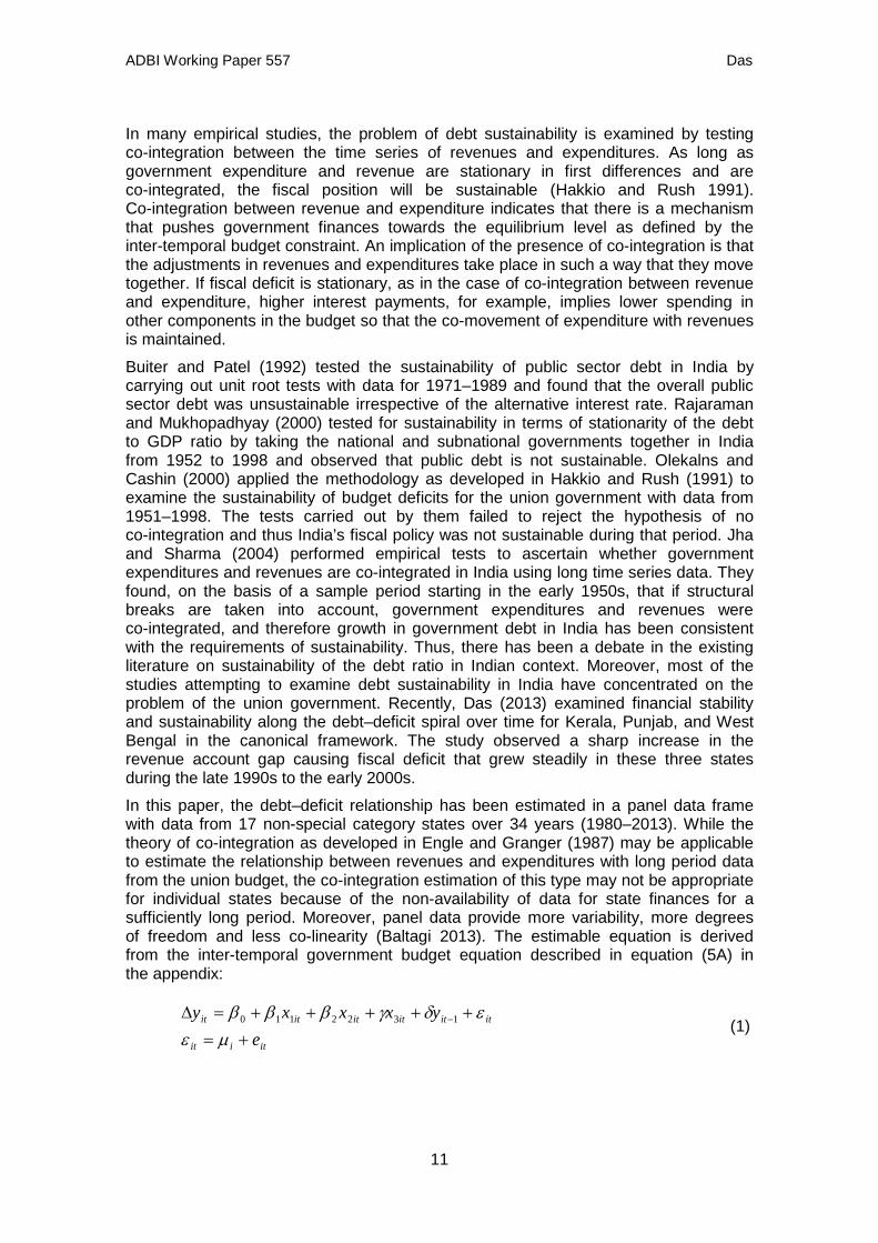
In many empirical studies, the problem of debt sustainability is examined by testing co-integration between the time series of revenues and expenditures. As long as government expenditure and revenue are stationary in first differences and are co-integrated, the fiscal position will be sustainable (Hakkio and Rush 1991). Co-integration between revenue and expenditure indicates that there is a mechanism that pushes government finances towards the equilibrium level as defined by the inter-temporal budget constraint. An implication of the presence of co-integration is that the adjustments in revenues and expenditures take place in such a way that they move together. If fiscal deficit is stationary, as in the case of co-integration between revenue and expenditure, higher interest payments, for example, implies lower spending in other components in the budget so that the co-movement of expenditure with revenues is maintained. Buiter and Patel (1992) tested the sustainability of public sector debt in India by carrying out unit root tests with data for 1971–1989 and found that the overall public sector debt was unsustainable irrespective of the alternative interest rate. Rajaraman and Mukhopadhyay (2000) tested for sustainability in terms of stationarity of the debt to GDP ratio by taking the national and subnational governments together in India from 1952 to 1998 and observed that public debt is not sustainable. Olekalns and Cashin (2000) applied the methodology as developed in Hakkio and Rush (1991) to examine the sustainability of budget deficits for the union government with data from 1951–1998. The tests carried out by them failed to reject the hypothesis of no co-integration and thus India’s fiscal policy was not sustainable during that period. Jha and Sharma (2004) performed empirical tests to ascertain whether government expenditures and revenues are co-integrated in India using long time series data. They found, on the basis of a sample period starting in the early 1950s, that if structural breaks are taken into account, government expenditures and revenues were co-integrated, and therefore growth in government debt in India has been consistent with the requirements of sustainability. Thus, there has been a debate in the existing literature on sustainability of the debt ratio in Indian context. Moreover, most of the studies attempting to examine debt sustainability in India have concentrated on the problem of the union government. Recently, Das (2013) examined financial stability and sustainability along the debt–deficit spiral over time for Kerala, Punjab, and West Bengal in the canonical framework. The study observed a sharp increase in the revenue account gap causing fiscal deficit that grew steadily in these three states during the late 1990s to the early 2000s. In this paper, the debt–deficit relationship has been estimated in a panel data frame with data from 17 non-special category states over 34 years (1980–2013). While the theory of co-integration as developed in Engle and Granger (1987) may be applicable to estimate the relationship between revenues and expenditures with long period data from the union budget, the co-integration estimation of this type may not be appropriate for individual states because of the non-availability of data for state finances for a sufficiently long period. Moreover, panel data provide more variability, more degrees of freedom and less co-linearity (Baltagi 2013). The estimable equation is derived from the inter-temporal government budget equation described in equation (5A) in the appendix:

itiit

itititititit

eyxxxy

+=+++++=∆ −

µεεδγβββ 1322110 (1)

11


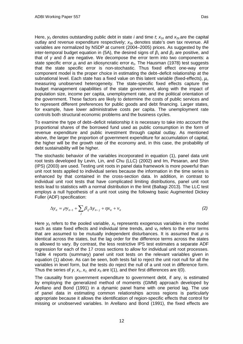
Here, yit denotes outstanding public debt in state i and time t; x1it and x2it are the capital outlay and revenue expenditure respectively; x3it denotes state’s own tax revenue. All variables are normalized by NSDP at current (2004–2005) prices. As suggested by the inter-temporal budget equation in (5A), the desired signs of β1 and β2 are positive, and that of γ and δ are negative. We decompose the error term into two components: a state specific error µi and an idiosyncratic error eit. The Hausman (1978) test suggests that the state specific error is non-stochastic. Thus fixed effect one-way error component model is the proper choice in estimating the debt–deficit relationship at the subnational level. Each state has a fixed value on this latent variable (fixed-effects), µi, measuring unobserved heterogeneity. The state-specific fixed effects capture the budget management capabilities of the state government, along with the impact of population size, income per capita, unemployment rate, and the political orientation of the government. These factors are likely to determine the costs of public services and to represent different preferences for public goods and debt financing. Larger states, for example, have lower administrative costs per capita. The unemployment rate controls both structural economic problems and the business cycles. To examine the type of debt–deficit relationship it is necessary to take into account the proportional shares of the borrowed fund used as public consumption in the form of revenue expenditure and public investment through capital outlay. As mentioned above, the larger the proportion of government expenditure for accumulation of capital, the higher will be the growth rate of the economy and, in this case, the probability of debt sustainability will be higher. The stochastic behavior of the variables incorporated in equation (1), panel data unit root tests developed by Levin, Lin, and Chu (LLC) (2002) and Im, Pesaran, and Shin (IPS) (2003) are used. Testing unit roots in panel data framework is more powerful than unit root tests applied to individual series because the information in the time series is enhanced by that contained in the cross-section data. In addition, in contrast to individual unit root tests that have complicated limiting distributions, panel unit root tests lead to statistics with a normal distribution in the limit (Baltagi 2013). The LLC test employs a null hypothesis of a unit root using the following basic Augmented Dickey Fuller (ADF) specification:

ititj

jitijitit vxyyy ++∆+=∆ ∑ −− ηβρ 1 (2)

Here yit refers to the pooled variable, xit represents exogenous variables in the model such as state fixed effects and individual time trends, and νit refers to the error terms that are assumed to be mutually independent disturbances. It is assumed that ρ is identical across the states, but the lag order for the difference terms across the states is allowed to vary. By contrast, the less restrictive IPS test estimates a separate ADF regression for each of the 17 cross sections to allow for individual unit root processes. Table 4 reports (summary) panel unit root tests on the relevant variables given in equation (1) above. As can be seen, both tests fail to reject the unit root null for all the variables in level form, but the tests do reject the null of a unit root in difference form. Thus the series of y, x1, x2, and x3 are I(1), and their first differences are I(0). The causality from government expenditure to government debt, if any, is estimated by employing the generalized method of moments (GMM) approach developed by Arellano and Bond (1991) in a dynamic panel frame with one period lag. The use of panel data in estimating common relationships across regions is particularly appropriate because it allows the identification of region-specific effects that control for missing or unobserved variables. In Arellano and Bond (1991), the fixed effects are

12


first eliminated by using first differences instead of the actual level of the variables and then an instrumental variable estimation of the differenced equation is performed. The lagged values of the endogenous variable or other variables which are correlated with the differenced error term, starting with lag two and potentially going back to the beginning of the sample are used as instrumental variables in the model. The overall validity of instruments is checked by the Sargan test of over-identifying restrictions.

Table 4: Estimated Statistics for Panel Unit Root Tests Series LLC t-statistics IPS W-statistics

yit –1.173 0.079 Δ yit –3.563 –4.863 x1it –3.332 –3.784 Δ x1it –10.060 –14.795 x2it 3.752 3.019 Δ x2it –11.046 –9.699 x3it –0.049 –1.874 Δ x3it –8.215 –11.969

Note: yit denotes debt-gdp ratio in state i and time t; x1it and x2it are the revenue expenditure and capital outlay relative to state’s income; x3it denotes state’s own tax revenue to state gdp ratio. Source: Author’s calculations with data from Reserve Bank of India. State Finances–A Study of Budgets, various years; Government of India, Central Statistics Office.

The estimated results shown in Table 5 suggest that the change in debt ratio is significantly more sensitive to revenue expenditure than capital expenditure at the subnational level. The elasticity of debt due to capital outlay was very little, but the government borrowing was highly attributable to public consumption in revenue account. Thus, a much larger fraction of the government debt has been used as revenue expenditure as public consumption at the subnational level. The increase in the states’ own tax revenue improved significantly the debt situation of the state governments. The coefficient for lagged debt ratio provides the nature of dynamics, but it is statistically insignificant. A higher level of expenditure, either in revenue account or capital account or both is the conventional reason for debt for every government. Public debt is also affected by some other factors relating to the capability of fiscal management of the government that are state specific and unobserved. The extent of debt escalating effect varied widely across the states because of the variation in fiscal performance of the subnational governments.

Table 5: Dynamic Panel Estimation of Debt and Government Spending Explanatory variables Coefficients z-statistics P>z

Intercept 0.227 2.52 0.012 log yit-1 0.023 0.51 0.607 log x1it 0.275 7.05 0.000 log x2it 0.005 1.79 0.073 log x3it –0.092 –2.88 0.004 Wald χ2(4) 60.31

Prob > χ2 0.0000 Source: Author’s calculations with data from Reserve Bank of India. State Finances–A Study of Budgets, various years;

Government of India, Central Statistics Office.

13


We observe that the increase in revenue expenditure has been mostly responsible for the higher level of borrowing at the subnational level in India. Government borrowing may be sustainable when it has a growth enhancing effect at a given cost per unit, the interest rate. Higher growth due to debt financed government expenditure could be the return from borrowing. This is because higher growth ultimately results in higher government revenues. Table 6 produces the estimates of growth enhancing effects of capital expenditure and revenue expenditure of the subnational governments in India. The results have been obtained by applying a one-way error component fixed effect model. I hypothesize that capital outlay has more growth enhancing effect than the revenue expenditure. But the estimated results shown in Table 6 fail to reject this hypothesis.

Table 6: Growth Effect of Borrowing by States Variables Coefficient t-statistics P>t

log x1it 3.1 2.830 0.005 log x2it 0.1 8.930 0.000 State-specific fixed effects Andhra Pradesh 16.3 21.860 0.000 Bihar 14.6 22.880 0.000 Chhattisgarh 15.9 21.300 0.000 Goa 13.4 19.980 0.000 Gujarat 16.6 20.900 0.000 Haryana 16.0 20.690 0.000 Jharkhand 15.8 21.480 0.000 Karnataka 16.1 21.490 0.000 Kerala 15.8 21.370 0.000 Madhya Pradesh 15.2 22.150 0.000 Maharashtra 17.6 21.310 0.000 Odisha 15.3 21.210 0.000 Punjab 15.8 21.470 0.000 Rajasthan 15.8 21.370 0.000 Tamil Nadu 16.6 21.810 0.000 Uttar Pradesh 16.4 22.250 0.000 West Bengal 16.7 21.730 0.000 Source: Author’s calculations with data from Reserve Bank of India. State Finances–A Study of Budgets, various years; Government of India, Central Statistics Office.

The growth elasticity of revenue expenditure is significantly higher than the elasticity of capital outlay. Again, as shown in Table 5, a larger proportion of government borrowing has been used in public consumption as revenue expenditure at the subnational level. In that sense, borrowings of the state governments have a growth enhancing effect, but the other way around. Government borrowing induced higher growth in states’ income mainly through the multiplier effect, not by raising public investment as such. The growth enhancing power of government borrowing has not been the same across the states. The growth effect of borrowing was the highest in Maharashtra and the lowest in Goa. In West Bengal, Gujarat, and Tamil Nadu, the growth effect was higher among the non-special category states. In Punjab, on the other hand, the growth effect was moderate while the incidence of borrowing for public consumption was high.

14


5. SUMMARY AND CONCLUSIONS This study describes the current fiscal health of the state governments in India in terms of the major deficit and debt indicators. Fiscal capacity, measured by its own tax ratio, varies considerably across the states. The tax ratio was the highest in Karnataka and the lowest in West Bengal in 2013–2014. There has also been a significant regional variation in the distribution of taxes collected by the union government as well as the grants provided by the central government. Perhaps, the most important indicator of fiscal health is revenue deficit, which was the highest in Haryana during 2013–2014, while Bihar exhibited the highest revenue surplus during the 2013–2014 fiscal year. The extent of borrowing used by the government for current expenditures is reflected in the primary deficit. All major states have recently experienced surplus in their primary fiscal balance. In 2013–2014, West Bengal generated the highest surplus in primary balance while experiencing significant fiscal deficit and the highest debt ratio among the non-special category states. While government debt and interest payments have no additional liability of the economy as a whole, larger interest payments have an adverse impact on income distribution and distort domestic demand in the form of higher consumption expenditure at the cost of capital accumulation and provision of public goods and services (Rakshit 2000). The interest payment liability of West Bengal was more than one-fifth of its revenue receipt, far above the interest liability of other non-special category states, during the fiscal period 2013–2014. While the states’ own revenue sources are not increasing fast enough to match their rising expenditure, the central devolution and other assistance are not adequate to cover the gap. Revenue deficits have widened and borrowings are being increasingly used to meet revenue expenditure. There has been a marked deterioration in the fiscal health of all states in India since the early 1990s, which reached a peak in the mid-2000s in almost every state in India. While the fiscal health of the state governments has improved recently, the debt ratio and interest payments are still alarming and the primary causes for growing debt ratio need to be analyzed. The expenditure side of the budget has a significant role in fiscal performance and government borrowing by influencing economic growth. The pattern of use of government borrowing is crucial as far as the sustainability of debt finance is concerned. The effects of government expenditures of different types on the debt to GDP ratio and on economic growth have been estimated after controlling for fixed state-specific effects. This study addresses the question of how different types of government spending are responsible for the rise in debt at the subnational level. The empirical findings suggest that the change in debt ratio is significantly more sensitive to revenue expenditure than capital expenditure at the subnational level. The increase in the states’ own tax revenue did not improve significantly the debt situation of the state governments. The growth elasticity of revenue expenditure is significantly higher than the elasticity of capital outlay. Thus, the borrowings of the state governments have a growth enhancing effect, but the other way round. The results also indicate that state-specific unobserved factors mostly related to the budget management capabilities of the state governments and the motivation of the political parties in power in the states have had a decisive impact on the rise in government borrowing and on economic growth of the states.

15


For a viable fiscal system, debt ratio should be sustainable over a long time. Debt will be sustainable when government consumption expenditure and transfer payments are to be met from revenue receipts of the government, while public investment and net government support to private investment should be financed through borrowing. The empirical findings of this study reject this hypothesis. In the empirical results expounded in this study, a growing debt ratio implies the inefficiency in fiscal management of the government in a sense that government spending on capital fails to contribute to the economic growth significantly. Thus, more emphasis is to be put on capital expenditure than on public consumption to make public debt sustainable at the subnational level.

16


REFERENCES Arellano, M. and S. Bond. 1991 Some Tests of Specification for Panel Data: Monte

Carlo Evidence and an Application to Employment Equations. Review of Economic Studies. 58. 277–297.

Barro, R. J. 1990. Government Spending in a Simple Model of Endogenous Growth. The Journal of Political Economy. 98 (5). S103–S125.

Baltagi, B. H. 2013. Econometric Analysis of Panel Data, 5th Edition. Chichester, United Kingdom: John Wiley & Sons Ltd.

Blanchard, O. J., J. C. Chouraki, R. P. Hagemann, and N. Sartor. 1990. The Sustainability of Fiscal Policy: New Answers to an Old Question. OECD Economic Studies. (15). 7–36.

Buiter, W. H. 1985. Guide to Public Sector Deficit and Debt. Economic Policy. November. 13–79.

Buiter, W.H. and U. R. Patel. 1992. Debt, Deficits and Inflation: An Application to the Public Finances of India. Journal of Public Economics. 47 (2). 171–205.

Chelliah, R. J. 2001. The Nature of the Fiscal Crisis in Indian Federation and Calibrating Fiscal Policy. ICRA Bulletin. Money and Finance. January–June. 52–75.

Das, N. 2013. Subnational-level Fiscal Health: Stability and sustainability implications for Kerala, Punjab, and West Bengal, IEG Working Paper No. 329.

Das, P. Forthcoming. Fiscal Deficit, Public Debt and Reforms–A Study of Subnational Finances in India: 1980–2013. The Journal of Income and Wealth.

Diamond, P. A. 1965. National Debt in a Neoclassical Growth Model. The American Economic Review. 55 (5). 1126–1150.

Domar, E. 1944. The Burden of Public Debt and National Income. American Economic Review. 34 (4). 798–827.

Engle, R. F. and C. W. J. Granger. 1987. Co-integration and Error Correction: Representation, Estimation, and Testing. Econometrica. 5. 251–276.

Government of India. 1994. Report of the Tenth Finance Commission (FOR 1995–2000). New Delhi: Finance Commission, Government of India,

Government of India. 2004. Report of the Twelfth Finance Commission (FOR 2005–2010). New Delhi: Finance Commission, Government of India.

Hakkio, C. S. and M. Rush. 1991. Is the Budget Deficit “Too Large?” Economic Inquiry. 29. 429–445.

Hausman, J. A. 1978. Specification Tests in Econometrics. Econometrica. 46 (6). 1251–1271.

Im, K. S., M. H. Pesaran, and Y. Shin. 2000. Testing Unit Roots in Heterogeneous Panels. Journal of Econometrics. 115. 53–74.

Jha, R. and A. Sharma. 2004. Structural Breaks, Unit Roots, and Cointegration: A Further Test of the Sustainability of the Indian Fiscal Deficit. Public Finance Review. 32, 220–231.

17

http://en.wikipedia.org/wiki/Jerry_A._Hausman

http://en.wikipedia.org/wiki/Econometrica


Keynes, J. M. 1980. Activities 1940–1946. Shaping the Post-War World: Employment and Commodities. In The Collected Writings of John Maynard Keynes, Vol. XXVII. London: Macmillan.

Levin, A., C. F. Lin, and C. Chu. 2002. Unit Root Tests in Panel Data: Asymptotic and Finite-Sample Properties. Journal of Econometrics. 108. 1–24.

Lucas, R. E. 1988. On the Mechanics of Economic Development. Journal of Monetary Economics. 22 (1). 3–42.

Olekalns, N. and P. Cashin. 2000. An Examination of the Sustainability of Indian Fiscal Policy. University of Melbourne, Department of Economics, Working Paper No.748, May.

Rajaraman, I. and A. Mukhopadhyay. 2000. Sustainability of Public Domestic Debt In India. National Institute of Public Finance and Policy Working Paper.

Rakshit, M. 2000. On Correcting Fiscal Imbalances in the Indian Economy Some Perspectives. Money and Finance. July–September 2000. 19–58.

Rangarajan, C. and D. K. Srivastava. 2005. Fiscal Deficits and Government Debt: Implications for Growth and Stabilisation. Economic and Political Weekly. 40 (27). 2919–2934.

Rankin, N. and B. Roffia. 2003. Maximum Sustainable Government Debt in the Overlapping Generations Model. The Manchester School. 71 (3). 217–241.

Reserve Bank of India. 2002. Report on Currency and Finance, 2000–01. New Delhi: Reserve Bank of India.

Romer, P. M. 1990. Endogenous Technological Change. Journal of Political Economy. 98 (5). S71–S102.

Singh, N. and G. Vasishtha. 2004. Patterns in Centre-State Fiscal Transfers – An Illustrative Analysis. Economic and Political Weekly. 39 (45). 489–493.

18


APPENDIX Domar’s model can be summarized in terms of the following inter-temporal budget constraint by assuming budget deficits are debt financed:

( ) 1

11

11

1 −

−−

−−

++=

−=+

−=−+

tttt

ttttt

tttttt

DrPDor

DDDrPor

DDRDrG

(1A)

Here, Gt is government spending (including transfer payment but excluding interest liability), Rt is government revenue, Dt is outstanding debt and rt is rate of interest in time t. Gt – Rt = Pt, the primary deficit. In this specification of dynamic budget constraint, the possibility to finance budget deficits through the creation of high-powered money is ruled away. This is because the subnational governments have no power to create money through the national central bank.6 Thus the subnational governments are more similar to a private borrower as they rely on some external source for the liquidity required to finance its expenditures in excess of revenues. By normalizing with GDP, Yt = (1 + gt)Yt-1, gt being the growth rate,

ttt

t

t

t

t

ttt

t

ttt Y

RYG

YP

pdgr

pd τγ −=−==

++

+= − ,11

1

(2A)

Equation (2A) suggests that the outstanding public debt is an accumulated sum of primary deficit and past stock of debt adjusted with the ratio of interest rate to GDP growth. Initially, Domar assumed that the economy's growth rate is exogenously given and is independent of public spending. The real interest rate is considered to be higher than the economy's growth rate. By subtracting dt-1 from both sides of equation (2A) yields,

11 −

+−

−−=∆ tt

ttttt d

grg

d τγ (3A)

The change in debt over time is the sum of primary deficit and, gap between growth rate and interest rate. When growth rate of GDP equals the interest rate, any increase in public debt would be the outcome of accumulated primary deficit only. As long as the rate of interest exceeds growth of GDP, debt stock will be more than the level of primary deficit. Thus the debt-stabilizing primary deficit is:

6 The possibility to finance public deficits by issuing high-powered money is excluded even if the government has a power to issue high-powered money because financing deficits through the creation of additional money would generate inflation in the long run. In a New Keynesian model, the increase in the supply of money generates inflation in so far as it raises aggregate demand and, hence, employment.

19


1*

1 −

+−

= tt

ttt d

grgp

(4A)

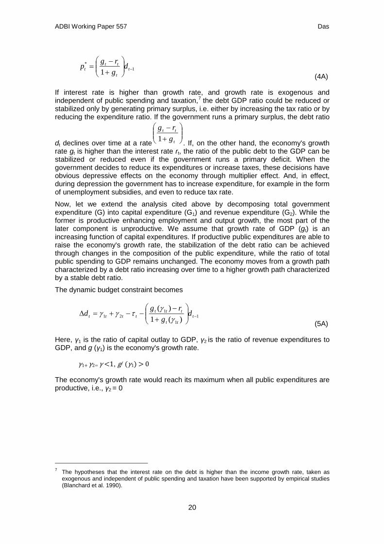
If interest rate is higher than growth rate, and growth rate is exogenous and independent of public spending and taxation,7 the debt GDP ratio could be reduced or stabilized only by generating primary surplus, i.e. either by increasing the tax ratio or by reducing the expenditure ratio. If the government runs a primary surplus, the debt ratio

dt declines over time at a rate

+−

t

tt

grg

1 . If, on the other hand, the economy's growth rate gt is higher than the interest rate rt, the ratio of the public debt to the GDP can be stabilized or reduced even if the government runs a primary deficit. When the government decides to reduce its expenditures or increase taxes, these decisions have obvious depressive effects on the economy through multiplier effect. And, in effect, during depression the government has to increase expenditure, for example in the form of unemployment subsidies, and even to reduce tax rate. Now, let we extend the analysis cited above by decomposing total government expenditure (G) into capital expenditure (G1) and revenue expenditure (G2). While the former is productive enhancing employment and output growth, the most part of the later component is unproductive. We assume that growth rate of GDP (gt) is an increasing function of capital expenditures. If productive public expenditures are able to raise the economy's growth rate, the stabilization of the debt ratio can be achieved through changes in the composition of the public expenditure, while the ratio of total public spending to GDP remains unchanged. The economy moves from a growth path characterized by a debt ratio increasing over time to a higher growth path characterized by a stable debt ratio. The dynamic budget constraint becomes

11

121 )(1

)(−

+

−−−+=∆ t

tt

ttttttt d

grg

dγ

γτγγ

(5A)

Here, γ1 is the ratio of capital outlay to GDP, γ2 is the ratio of revenue expenditures to GDP, and g (γ1) is the economy's growth rate.

γ1+ γ2= γ <1, g/ (γ1) > 0

The economy's growth rate would reach its maximum when all public expenditures are productive, i.e., γ2 = 0

7 The hypotheses that the interest rate on the debt is higher than the income growth rate, taken as exogenous and independent of public spending and taxation have been supported by empirical studies (Blanchard et al. 1990).

20

Documents

Debt Dynamics, Fiscal Deficit, and Stability in Government Borrowing in India: A Dynamic Panel Analysis