Embed Size (px)
Citation preview

econstorMake Your Publications Visible
A Service of
zbwLeibniz-InformationszentrumWirtschaftLeibniz Information Centrefor Economics
Kapeller Jakob Schuumltz Bernhard
Working Paper
Debt Boom Bust A Theory of Minsky-VeblenCycles
Working Paper No 1214
Provided in Cooperation withJohannes Kepler University of Linz Department of Economics
Suggested Citation Kapeller Jakob Schuumltz Bernhard (2012) Debt Boom Bust A Theoryof Minsky-Veblen Cycles Working Paper No 1214 Johannes Kepler University of LinzDepartment of Economics Linz
This Version is available athttphdlhandlenet1041973601
Standard-Nutzungsbedingungen
Die Dokumente auf EconStor duumlrfen zu eigenen wissenschaftlichenZwecken und zum Privatgebrauch gespeichert und kopiert werden
Sie duumlrfen die Dokumente nicht fuumlr oumlffentliche oder kommerzielleZwecke vervielfaumlltigen oumlffentlich ausstellen oumlffentlich zugaumlnglichmachen vertreiben oder anderweitig nutzen
Sofern die Verfasser die Dokumente unter Open-Content-Lizenzen(insbesondere CC-Lizenzen) zur Verfuumlgung gestellt haben solltengelten abweichend von diesen Nutzungsbedingungen die in der dortgenannten Lizenz gewaumlhrten Nutzungsrechte
Terms of use
Documents in EconStor may be saved and copied for yourpersonal and scholarly purposes
You are not to copy documents for public or commercialpurposes to exhibit the documents publicly to make thempublicly available on the internet or to distribute or otherwiseuse the documents in public
If the documents have been made available under an OpenContent Licence (especially Creative Commons Licences) youmay exercise further usage rights as specified in the indicatedlicence
wwweconstoreu
DDEEPPAARRTTMMEENNTT OOFF EECCOONNOOMMIICCSS
JJOOHHAANNNNEESS KKEEPPLLEERR UUNNIIVVEERRSSIITTYY OOFF
LLIINNZZ
Johannes Kepler University of Linz Department of Economics
Altenberger Strasse 69 A-4040 Linz - Auhof Austria
wwweconjkuat
bernhardschuetzjkuat phone +43 (0)732 2468 8584 -9679 (fax)
Debt Boom Bust A Theory of Minsky-Veblen Cycles
by
Jakob KAPELLER Bernhard SCHUumlTZ)
Working Paper No 1214 December 2012
Debt Boom Bust
A Theory of Minsky-Veblen Cycles
Jakob Kapellerlowast
Bernhard Schutzdagger
Abstract
This paper reflects on the development leading to the recent crisis and interprets this
development as a series of events within a Minsky-Veblen Cycle To illustrate this claim
we introduce conspicuous consumption concerns as described by Veblen into a stock flow
consistent Post Keynesian model and demonstrate that under these conditions a decrease
in income equality leads to a corresponding increase in debt-financed consumption demand
Here Minskyian dynamics come into play increased credit demand leads to a corresponding
rise in credit supply which eventually gives rise to a debt-financed consumption boom
As the solvency of households decreases and interest rates move up banks reduce lending
triggering household bankruptcies and finally a recession What follows is a stable period
of consolidation where past debts are repaid financial stability is regained and conspicuous
consumption motives may gradually take over again We illustrate this approach to the
current crisis and its explanatory validity by extending our stock-flow consistent model into
a dynamic simulation
JEL classification numbers B52 D11 E12 E20 G01
lowastUniversity of Linz Department of Philosophy and Theory of Science Altenbergerstrasse 69 4040 Linz Aus-
tria email jakobkapellerjkuat phone +43 732 2468 3685daggerUniversity of Linz Department of Economics Altenbergerstrasse 69 4040 Linz Austria email Bern-
hardSchuetzjkuat phone +43 732 2468 8584
1
DEBT BOOM BUST A THEORY OF MINSKY-VEBLEN CYCLES
1 Introduction
If one was asked by an educated layperson about the best way to understand the rdquocurrent crisisrdquo
which already has evolved from a financial or private debt crisis to a sovereign debt crisis we
claim that one legitimate answer would be the following
First read Thorstein Veblenrsquos seminal book The Theory of the Leisure Class (espe-
cially chapters 4-5) and pay attention to the remarkable increase in income inequality
in the US during the last decades This might convince you that relative consump-
tion concerns are an important factor for explaining why so many households were
willing to take up so much debt Second read the book by Hyman Minsky called
Stabilizing an Unstable Economy (in particular chapters 9-10) and you will under-
stand which immanent forces breed the emergence of instruments such as CDSrsquo and
CDOrsquos within the banking system to meet additional credit demand and lead almost
by necessity to ever riskier loan provision and gradually move the system from a
state of relative stability to a state of extreme fragility and crisis Finally take a
look in John Maynard Keynesrsquo The General Theory of Employment Interest and
Money (chapter 3 should suffice at least for the moment) to get a rough under-
standing of the principle of effective demand and the macroeconomic consequences
for employment and income
Any reader instructed this way is possibly quite astonished when stumbling on the publishing
dates of these books (1899 1936 1986) and one is inclined to ask how such a crisis can emerge
unnoticed if these books already pointed to what had to be expected
The purpose of this paper is to explore and to validate this story by illustrating how the US
economy (as well as many European economies) finds itself in the middle of a Minsky-Veblen
Cycle In doing so we draw on the path-breaking contributions on stock flow consistent modeling
by Lavoie and Godley (2002) and Godley and Lavoie (2007) By bringing together concepts
from different origins - the InstitutionaryEvolutionary concept of relative consumption concerns
(Veblen) and Keynesian ideas on the nature of financial markets (Minsky) - it contributes to a
Pluralist Paradigm in the spirit of Dobusch and Kapeller (2012) that seeks to create new insights
through the exploitation of complementary concepts as they are found in different schools of
thought1
1Other approaches that try to incorporate the Veblenian idea of conspicuous consumption in Post Keynesianmodels are eg Barba and Pivetti (2009) Dutt (2005 2006 2008) Hein (2012) Kapeller and Schutz (2012) andZezza (2008)
2
DEBT BOOM BUST A THEORY OF MINSKY-VEBLEN CYCLES
The paper is structured as follows Section 2 presents the basic theoretical arguments put
forth by Veblen (1970 [1899]) and Minsky (1986) as well as some stylized facts emphasizing
the importance of these concepts for understanding the current crisis Section 3 introduces a
theoretical model incorporating and accounting for these insights In section 4 we dynamically
extend our model to provide simulation results for different scenarios illustrating the mechanisms
giving rise to the existence of Minsky-Veblen cycles Section 5 concludes the paper
2 Income inequality debt and crisis Theoretical perspectives
and stylized facts
The pivotal role of the increase in income inequality in the US as one of the main causes of the
recent crisis is widely acknowledged and discussed extensively (see eg Barba and Pivetti 2009
Evans 2009 ILO and IMF 2010 Kumhof et al 2012 Kumhof and Ranciere 2010 Rajan 2010
Stiglitz 2009 UN Commission of Experts 2009 van Treeck 2012) Figure 1 shows how family
incomes diverged during the last 30 years thereby reversing the process of convergence taking
place in the prior 30 years
Figure 1 Real family income growth by quintiles
1174
9791035 1047
887
37-74
112
227
490
-200
00
200
400
600
800
1000
1200
1400
Lowest fifth Second fifth Third fifth Fourth fifth Highest fifth
1947-1973 1979-2009
Source State of Working America EPI analysis of Census Bureau data
3
DEBT BOOM BUST A THEORY OF MINSKY-VEBLEN CYCLES
When inequality increases people may find it hard to sustain a rdquoconventionalrdquo living standard
which is often perceived as a living standard comparable to the people one associates with
(friends neighbors colleagues family members) that is the people with whom we share our
social identity (Hogg and Terry 2000) These people serve as reference standards as rdquoprotoypesrdquo
(Kahneman et al 1991) so to say insofar as they influence the consumption aspirations of their
associates In this context Veblen (1970 [1899]) emphasized the ubiquity of relative consumption
concerns thereby ascribing a central role to the social mediation of preferences Following this
argument the primary reason why people suffer from a reduction in their level of consumption
relative to others is not to be found in the alleged loss of comfort or arousal that goes with it
but in the loss of social status in the broadest sense Following that argument people define
themselves relative to the (visible) consumption of their neighbors and colleagues (or other
people they closely associate with) In this sense conspicuous consumption is far from being
identical to envy or greed but is ultimately about social belonging and the social conventions
associated with carrying a specific social identity
For the great body of people in any modern community the proximate ground of
expenditure in excess of what is required for physical comfort [] is a desire to
live up to the conventional standard of decency in the amount and grade of goods
consumed (Veblen 1970 [1899] p 80)
No class of society not even the most abjectly poor forgoes all customary conspic-
uous consumption The last items of this category of consumption are not given up
except under the stress of the direst necessity Very much of squalor and discomfort
will be endured before the last pretense of pecuniary decency is put away (Veblen
1970 [1899] p 70)
Applying this argument to recent developments implies that an increase in income inequality will
induce some of the disadvantaged people to reduce their saving rate or ndash if this is not sufficient
to realize onersquos consumption aspirations ndash go into debt2 Additionally he argues that social
comparisons across the social scale will exhibit an upward tendency since
[] each class envies and emulates the class next above it in the social scale while
it rarely compares itself with those below or with those who are considerably in
advancerdquo (Veblen 1970 [1899] p 81)
2Half a century later Duesenberry (1962[1949]) arrived at a similar conclusion though he argued that the fall inthe saving rate is caused by the desire of people for superior goods which stem from the continual improvementof consumption goods rdquoFor any particular family the frequency of contact with superior goods will increaseprimarily as the consumption expenditure of others increase When that occurs impulses to increase expenditurewill increase in frequency and strength and resistance to them will be inadequate The result will be an increasein expenditure at the expense of savingrdquo (Duesenberry 1962[1949] p 27)
4
DEBT BOOM BUST A THEORY OF MINSKY-VEBLEN CYCLES
Evidence for the empirical relevance of conspicuous consumption and its connection to the in-
creasing indebtedness of US households can be found in Boushey and Weller (2006) Bowles
and Park (2005) Christen and Morgan (2005) Krueger and Perri (2006) Neumark and Postle-
waite (1998) Pollin (1988 1990) and Schor (1998)3 See also van Treeck (2012) who provides
an accessible overview of the main results
While these results imply that there was considerable demand for credit in the pre-crisis period
high demand for credit as such hardly increases the fragility of the financial system if it is
not accommodated by a corresponding increase in credit supply This crisis has been called
a Minsky moment at various occasions (see eg McCulley 2009 The Economist 2009 The
Financial Times 2007 The New Yorker 2008 The Wall Street Journal 2007 Whalen 2007)
since both the deregulation of financial markets (culminating eg in the repeal of the Glass-
Steagall Act) as well as the rise of financial rdquoinnovationsrdquo like Credit Default Swaps (CDS) and
Collateralized Debt Obligations (CDOs) allowing profit seeking bankers to create an ever rising
flow of loans to people who could not afford them are strongly reminiscent of Minskyrsquos works
Following Minsky this type of development is a quite natural aftermath of a period of relative
stability4
A period of successful functioning of the economy leads to a decrease in the value
of liquidity and to an acceptance of more aggressive financing practices Banks
nonbank financial institutions and money-market organizations can experiment with
new liabilities and increase their asset-equity ratio without their liabilities losing any
significant credence (Minsky 1986 p 249)
Margins of safety continuously decrease in a period of financial stability rdquoas success leads to a
belief that the prior - and even the present - margins are too largerdquo (Minsky 1986 p 220) Sim-
ilarly regulatory obligations erode as the financial system develops strategies and instruments
to evade them
3Pollin (1988 1990) concludes that the increase in household indebtedness beginning in the early 1970s was dueto efforts to maintain past living standards in a period of low wage growth Neumark and Postlewaite (1998) findthat women whose sisterrsquos husband earns a higher income are more likely to seek paid employment Schor (1998)found during interviews that the relative financial position of workers to their reference group had a significantimpact on their saving rate Bowles and Park (2005) report a significant positive impact of income inequality onworking hours and Christen and Morgan (2005) and Boushey and Weller (2006) find that higher income inequalityleads to an increase in household debt Krueger and Perri (2006) find that an increase in income inequality doesnot lead to an increase in consumption inequality
4See also Kindleberger (1978) on how institutional innovations or rearrangements leading to an increasedsupply of credit are a general feature of financial euphoria and crises
5
DEBT BOOM BUST A THEORY OF MINSKY-VEBLEN CYCLES
The profit-seeking bankers almost always win their game with the authorities but in
winning the banking community destabilizes the economy the true losers are those
who are hurt by unemployment and inflation (Minsky 1986 p 250)
Furthermore a housing price bubble led banks to lend against asset values instead of the bor-
rowers income (McCulley 2009) which contributed significantly to the destabilization of the
financial system
A cash-flow orientation by bankers is conducive to sustaining a robust financial struc-
ture An emphasis by bankers on the collateral value and the expected values of assets
is conducive to the emergence of a fragile financial structure (Minsky 1986 p 234)
From this it follows that households which initially start out as hedge financing units (who
could pay interest and principal out of current income) gradually turn into speculative financing
(who can only pay the interest but not the principal out of current income) or Ponzi financing
units (who can neither repay interest nor principal out of current income) This development is
further accelerated by a rise in interest rates and the burst of asset bubbles
All of this resembles very much the developments observed before and during the crisis (see
McCulley 2009) Banks found new ways to increase profitability and circumvent regulation by
granting mortgage loans to people who were hardly creditworthy (subprime mortgages) bundling
these loans and selling them This system could continue as long as house prices and therefore
collateral values kept rising As the overvaluation became all too apparent (see on this also
Shiller 2005) the housing bubble burst In turn banks reduced lending which in combination
with fallen collateral values caused speculative- and Ponzi-financing units to default inflicting
huge losses on the financial sector Eventually this development culminated in a financial crisis
that quickly spread around the globe and into the real economy causing the worst recession
since the Great Depression
3 A stock-flow consistent framework for exploring Minsky-Veblen
Cycles
In this section we incorporate the Veblenian and Minskyan concepts introduced above in a stock
flow consistent accounting framework as developed by Lavoie and Godley (2002) and Godley
and Lavoie (2007) This method allows us to keep track of stock developments and to ensure
that all flows and money stocks within our model economy add up to zero thereby avoiding
6
DEBT BOOM BUST A THEORY OF MINSKY-VEBLEN CYCLES
model inconsistencies For simplicity we assume a closed economy without taxes and government
spending Aggregate output Y is the sum of the supplies of investment and consumption goods
where we assume that within each short period supply equals demand
Y (t) = Cd(t) + Id(t) (1)
Furthermore we assume three distinct classes capitalists workers whose share in aggregate
income remains constant (we will simply refer to them as type 1 workers) and workers whose
income share is decreasing (type 2 workers) Workers receive wage income as well as interest
income on (positive) money deposits which makes their disposable income (Y Dw)
Y Dwi(t) = wi(t)Ndwi(t) + λMwi(tminus 1) (2)
λ =
Mwi(tminus 1) ge 0 rD
Mwi(tminus 1) lt 0 rL + φ
Here i = 1 2 denotes workers of type 1 or 2 wi the real wage rate and Ndwi the respective
employment level When workers are saving they accumulate deposits Mwi on which they
receive interest payments In this case r = rD If workers decide to spend more than their
disposable income they reduce their deposits Mwi If Mwi is depleted workers can take up
loans which is expressed by negative values of Mwi In such a case r = rL (where rL gt rD)
and they additionally repay a part φ of the principal each period Capitalists receive distributed
profits from firms and banks as well as interest income on their (positive) deposits Thus their
disposable income is equal to
Y Dc(t) = πfΠf (t) + πbΠb(t) + λMc(tminus 1) (3)
λ =
Mc(tminus 1) ge 0 rD
Mc(tminus 1) lt 0 rL + φ
πf and πb are the ratios of distributed firm and bank profits and Πf and Πb denote firm and
bank profits Unlike profits losses remain within the firm resp banking sector which means
πf = 0 if Πf lt 0 as well as πb = 0 if Πb lt 0 Like workers they can also spend more than their
disposable income by depleting their money balances or taking up loans in which case they too
have to pay interest and repay part φ of the principal each period
7
DEBT BOOM BUST A THEORY OF MINSKY-VEBLEN CYCLES
We assume that the ratio of type 1 and type 2 workers employed in the production process
(β = Ndw2N
dw1) remains constant This leaves us with the following labor demand functions
Ndw1(t) =
Y (t)
PR
1
1 + βNd
w2(t) =Y (t)
PR
β
1 + ββ = Nd
w2Ndw1 (4)
For simplicity labor productivity (PR) is assumed constant Workers will always consume
at least subsistence level consumption where a0 denotes the aggregate subsistence level con-
sumption of the working class Furthermore workers consume fraction a1 of disposable income
exceeding the necessary amount for subsistence level consumption In case of type 1 workers
this leaves us with the following consumption function
Cdw1(t) =
1
1 + βa0 + a1
[Y Dw1(t)minus
1
1 + βa0
](5)
where 1(1 + β)a0 is the amount of subsistence level consumption related to type 1 workers
Consumption demand cannot fall below the subsistence level therefore Cdw1(t) = 1(1+β)a0 for
Y Dw1(t) lt 1(1 + β)a0 As indicated above we assume that consumer preferences are socially
mediated Specifically in what follows we assume that one group of workers (type 2 ) suffers
a decline in wages relative to the other group (type 1 ) but partly still tries to keep up with
the latter group in terms of consumption expenditures In Veblenian terms this scenario posits
that type 2 workers become a somewhat rdquolowerrdquo class and therefore change their behavior ie
their preferred ratio of consumption aspirations to current income while it leaves the behavior
of type 1 workers (becoming a superior class) relatively unaffected (see Veblen 1970 [1899]) In
line with this argument we assume that as long as disposable income of type 2 workers is at
least as high as those of type 1 workers ie Y Dw2 ge Y Dw1(t)β the consumption function of
type 2 workers looks similar to their type 1 counterparts
Cdw2(t) =
β
1 + βa0 + a1
[Y Dw2(t)minus
β
1 + βa0
](6)
where β(1 + β)a0 is the amount of subsistence level consumption of type 2 workers and sim-
ilar to above consumption demand cannot fall below β(1 + β)a0 However as soon as their
income drops below their peersrsquo income ie Y Dw2(t) lt YDw1(t)β an additional type of social
interaction emerges which is the desire to keep up with type 1 workers
Cdw2(t) = (1minus α)
(β
1 + βa0 + a1
[Y Dw2(t)minus
β
1 + βa0
])+ αCd
w1(t)β (7)
8
DEBT BOOM BUST A THEORY OF MINSKY-VEBLEN CYCLES
While consumption behavior as described in equation (6) is still present in equation (7) the
latter also introduces relative consumption concerns where the relative importance of these two
motives is given by α If α = 1 relative consumption concerns fully determine consumer behavior
implying that workers would exactly hold on to the consumption level of type 1 workers while
in the case of α = 0 equation (7) reduces to equation (6) ie relative consumption concerns
would be irrelevant for individual consumer behavior In general the higher the desire to keep
up with the other group the larger will be α (see Kapeller and Schutz 2012)
The composition of capitalist consumption demand on the other hand is much simpler and given
by
Cdc (t) = b0 + b1 [Y Dc(t)minus b0] (8)
where we assume b1 lt a1
Investment depends on the past utilization rate (z = YY lowast) and the past rate of return (RR =
ΠfK)
Id(t) = i0 + i1z(tminus 1) + i2RR(tminus 1) (9)
Here K denotes the capital stock and Y lowast full capacity output which is determined by the capital
stock according to Y lowast = νK where ν is assumed constant
The capital stock evolves over time following
K(t) = K(tminus 1) + Is(tminus 1)minus δK(tminus 1) (10)
where δ denotes the depreciation rate
Profits of the firm and the banking sector are given by
Πf (t) = Y (t)minus w1(t)Ndw1(t)minus w2(t)N
dw2(t) + λMf (tminus 1) (11)
λ =
Mf (tminus 1) ge 0 rD
Mf (tminus 1) lt 0 rL + φ
9
DEBT BOOM BUST A THEORY OF MINSKY-VEBLEN CYCLES
Πb(t) = minus[rMw1(tminus 1) + rMw2(tminus 1) + rMc(tminus 1) + rMf (tminus 1)]minus cancel(t) (12)
where in (12) r = rL if the respective sectorrsquos money balance is negative and r = rD otherwise
cancel denotes debt cancelations in case of bankruptcies of clients Since workers do not receive
loans indefinitely we assume that loans are granted as long as workersrsquo income exceeds payments
on past loans plus a certain margin of safety θ
wwi(t)Ndwi(t) ge minus [rL(t) + φ]Mwi(tminus 1) + θwi(t) (13)
We express the initial margin of safety (in a Minskyan fashion it will be subject to change) in
multiples of subsistence level consumption a0 such that in case of type 2 workers its initial level
is given by
θw2(0) = η
[β
1 + βa0
](14)
where larger values of η imply more cautious banks This specification allows for a direct
comparison between a householdrsquos financial status as envisaged by the financial sector and the
Minskyan conditions for distinguishing hedge and speculativePonzi financing units Following
this line of argument our type 2 workers are hedge financing units as long as condition (15)
holds and turn into speculative financing units when condition (15) is violated In this case they
remain speculative financing units as long as condition (16) holds and turn into Ponzi financing
units if condition (16) is violated
Y Dw2 geβ
1 + βa0 (15)
Y Dw2 geβ
1 + βa0 + φMw2(tminus 1) (16)
Similar to households also banks are assumed to behave according to Minskyan propositions
thereby (slowly) relaxing the margin of safety in times of financial stability and (rapidly) in-
creasing the very same margin in cases of financial distress Specifically we assume that if no
bankruptcies occur during a certain period θ will decrease with rate γ whereas in case of re-
ported customer bankruptcies it jumps up by τθ (where τ gt γ) This reflects the Minskyan
argument that during periods of economic stability financial intermediaries become gradually
less cautious until bankruptcies lead to a sudden readjustment of risk perceptions thereby pos-
10
DEBT BOOM BUST A THEORY OF MINSKY-VEBLEN CYCLES
sibly creating a credit crunch Additionally banks are assumed to get more cautious when the
total amount of private debt (L) which is the absolute value of negative deposits increases (and
vice versa)
θ(t) = θ(tminus 1)(1 + micro) + ζ∆L(t) (17)
where micro = minusγ in periods where no case of bankruptcy occurs and micro = τ in periods of bankrupt-
cies Our conception of θ is thereby quite flexible While a fall in θ can be due to profit
seeking bankers becoming gradually less cautious (due to various reasons discussed by Minsky)
or find new ways to circumvent regulation it can also be due to a housing price bubble which
may increase γ when loan officers begin lending against asset values instead of current income
also implying a decrease in the margin of safety5 This conceptual flexibility distinguishes it
from other Minskyan models (see Dos Santos 2005 Keen 1995 2011 Palley 1994 Taylor and
OrsquoConnell 1985 Tymoigne 2006)
If bank clients are bankrupt ndash ie they become credit constrained and their income after debt
payments is not enough to afford subsistence level consumption ndash we assume that banks have to
write off a fixed proportion χ of their claims From the point of view of workers this looks like
∆Mwi = minusχMwi = cancelwi (18)
Generally workers will always consume at least subsistence level consumption If their income
is not sufficient to afford subsistence level consumption and debt payments workers will first
suspend debt repayments and then interest rates Following Minsky (1986) the interest rate on
loans depends positively on the amount of debt in the economy
rL = rL(tminus 1) + ρ∆L(t) (19)
Table 1 and 2 provide an overview of all flows and stocks incorporated in our model
5See Zezza (2008) for the implementation of the housing market in a stock-flow consistent model
11
DEBT BOOM BUST A THEORY OF MINSKY-VEBLEN CYCLES
Table 1 Stock matrix
Households Firms Bankssum
Worker 1 Worker 2 Capitalists
Money deposits +Mw1 +Mw2 +Mc +Mf minusM 0
Fixed capital +K K
Balance (net-worth) minusVw1 minusVw2 minusVc minusVf minusVb minusKsum0 0 0 0 0 0
Note that M = Mw1 + Mw2 + Mc + Mf Subtracting net worth assures that columns and rows add up
to zero The only row not adding up to zero relates to the capital stock which is the only stock that is
only an asset and not a liability at the same time See Godley and Lavoie (2007) for further details
12
DEBT BOOM BUST A THEORY OF MINSKY-VEBLEN CYCLES
Table
2
Flo
wm
atr
ix
House
hold
sF
irm
sB
anks
sumW
ork
er1
Work
er2
Capit
alist
sC
urr
ent
Capit
al
Curr
ent
Capit
al
Consu
mpti
on
minusC
d w1(t
)minusC
d w2(t
)minusC
d c(t
)+C
s(t
)0
Invest
ment
+Is(t
)minusId(t
)0
[Pro
ducti
on]
[Y(t
)]
Wages
+w
1(t
)Nw1(t
)+w
w2(t
)Nw2(t
)minusw
1(t
)Nw1(t
)0
minusw
w2(t
)Nw2(t
)
Inte
rest
+rM
w1(tminus
1)
+rM
w2(tminus
1)
+rM
c(tminus
1)
+rM
f(tminus
1)
minusrM
w1(tminus
1)
0minusrM
w2(tminus
1)
minusrM
c(tminus
1)
minusrM
f(tminus
1)
Repaym
ent
+φM
w1(tminus
1)
+φM
w2(tminus
1)
+φM
c(tminus
1)
+φM
f(tminus
1)
0minusφM
w1(tminus
1)
minusφM
w2(tminus
1)
minusφM
c(tminus
1)
minusφM
f(tminus
1)
Debt
Cancela
tion
minusχM
w1(tminus
1)
minusχM
w2(tminus
1)
minusχM
c(tminus
1)
+χM
w1(tminus
1)
0+χM
w2(tminus
1)
+χM
c(tminus
1)
Pro
fits
+πfΠ
f(t
)+πbΠ
b(t
)-Π
f(t
)+
(1minusπf)Π
f(t
)-Π
b(t
)+
(1minusπb)Π
b(t
)0
∆D
ep
osi
tsminus
∆M
w1(t
)minus
∆M
w2(t
)minus
∆M
c(t
)minus
∆M
f(t
)+
∆M
(t)
0sum
00
00
00
00
The
sup
ersc
rip
tsd
ands
den
ote
dem
and
and
sup
ply
N
ote
thatC
=C
w1
+C
w2
+C
candM
=M
w1
+M
w2
+M
c+M
fth
at
for
the
resp
ecti
vese
ctor
r=r D
ifit
sm
oney
bal
ance
isp
osit
ive
andr
=r L
oth
erw
ise
Note
furt
her
that
for
the
resp
ecti
vese
ctorφ
=0
ifit
sm
oney
bala
nce
isp
osi
tive
and
that
rep
aym
ent
ofdeb
tis
don
eou
tof
curr
ent
inco
me
(an
den
ters
wit
ha
posi
tive
sign
since
money
dep
osi
tsare
neg
ati
ve
for
ind
ebte
dh
ouse
hold
s)and
isca
nce
led
out
inth
esa
me
colu
mn
sin
cere
pay
men
tsgo
dir
ectl
yin
toth
ere
spec
tive
dep
osi
ts
Note
finally
that
all
row
san
dco
lum
ns
add
up
toze
ro
assu
ring
the
mod
elrsquos
stock
-flow
con
sist
ency
See
Godle
yan
dL
avoie
(2007)
for
furt
her
det
ails
13
DEBT BOOM BUST A THEORY OF MINSKY-VEBLEN CYCLES
4 Simulation results
This section presents a simulation of a dynamic version of the stock-flow consistent model intro-
duced in the previous section All simulations have been run for 420 periods where one period
is treated as equal to a quarter of a year Graphical representations of our main simulation
results can be found in figure 2 and 3 All starting values and parameter specifications used in
this paper are supplied in Appendix A Appendix B reproduces the exact Mathematica code
which has been used for generating the simulations presented below
In what follows we distinguish four scenarios In the first scenario ndash our baseline case ndash we
assume that no increase in inequality occurs leaving the economy on a stable path The second
scenario shows the effects of an increase in inequality without any social mediation of prefer-
ences ndash here growth rates are negative which is in line with the standard results concerning
consumption-driven economies in Post Keynesian models The third scenario modifies the sec-
ond by incorporating relative consumption concerns which in contrast to the second scenario
leads to a significant growth in output due to debt-financed private consumption While the
third scenario does not impose any limits in credit supply the fourth scenario introduces bank
behavior modelled according the theoretical premises sketched above leading to the alleged
Minsky-Veblen Cycles
41 Scenario 1 ndash The Baseline Case
In our baseline scenario we assume that the household sector holds all positive deposits while
firms hold all liabilities Wages and interest rates are assumed constant where the initial wage
share is assumed to be 68 and bank equity as well as workersrsquo deposits are initially zero
Output shows a marginal upward trend which is due to capitalists spending their savings in
order to finance their lifestyle Capitalistrsquo expenditures allow workers to increase their deposits
and firms to have positive profits We assume that banks distribute all of their profits to
capitalistrsquo households while firms retain 10 percent of their profits
42 Scenario 2 ndash Increasing inequality in the absence of relative consumption
concerns a case of contraction
Next we assume a gradual decrease of wages of type 2 workers taking place in the first 8 periods
leading to a decline in the wage share to 65 solely at the expense of type 2 workers Relative
consumption concerns are absent in this scenario (α = 0) leading to a downswing in output due
14
DEBT BOOM BUST A THEORY OF MINSKY-VEBLEN CYCLES
to reduced consumption spending of type 2 workers Consequentially this scenario looks similar
to the previous but stabilizes at a lower level of aggregate income
43 Scenario 3 ndash Increasing inequality in the presence of relative consumption
concerns a case of expansion
Here we replicate the decrease in wages of type 2 workers under the assumption that the social
mediation of preferences has a strong impact on individual consumer behavior (α = 08) In
this case the decline in wages causes the saving rate of type 2 workers to decrease becoming
negative from the third period onwards Let us for now leave aside Minskyan dynamics expressed
in equations (13)-(19) and assume an infinite supply of credit (θ = minusinfin) and a constant interest
rate (rL = rL(0)) In this case overconsumption of type 2 workers leads to an initial expansion
As debt payments increase and disposable income falls type 2 workers gradually reduce their
consumption bringing the expansion to a quick end Nevertheless overconsumption is sufficient
to keep output at a high level However when reaching their subsistence level workers cannot
further reduce consumption Here disposable income has already turned negative meaning that
workers have already turned into Ponzi financing units that depend on banks rolling over credit
With debt and interest payments increasing without workers being able to reduce consumption
any further this creates a second expansion at the end of the scenario which follows a pure
Ponzi scheme Type 2 households are taking up new loans to make debt payments on outstanding
loans causing debt obligations to rise even further and creating ever increasing flows of interest
payments manifesting itself in ever increasing bank profits These profits which lead to an
increase in capitalist consumption that is the source of the subsequent boom are of course only
artificial since the underlying rdquocash flowsrdquo are generated by the banking system itself and no
one can expect those loans to be ever repaid
44 Scenario 4 ndash The case of rdquoMinsky-Veblen Cyclesrdquo
Of course the possibility of such a prolonged boom is quite unrealistic At some point banks
have to admit that those loans can never be repaid necessarily leading to a rapid decline of
credit supply Interest rates are also likely to increase in such a scenario Therefore we add the
Minskyan dynamics introduced in equations (13)-(19) and discuss three variants of this scenario
where each variant assumes a different level of cautiousness in the banking sector
15
DEBT BOOM BUST A THEORY OF MINSKY-VEBLEN CYCLES
441 Scenario 4a ndash Minsky-Veblen Cycles and Speculative Dynamics
In every variant of scenario 4 the decrease in the wage rate of type 2 workers causes an initial
boom We assume that η = 12 meaning that at the beginning banks do grant loans as long as
type 2 workers have sufficient disposable income to pay for 12 times the amount of subsistence
level consumption ie θw2(0) = 12 [β(1 + β)a0]
As wages of type 2 workers decrease we initially observe the same debt financed boom as in the
third scenario When debt payments increase workers gradually reduce consumption leading
to a small recession and a phase of stagnation Nevertheless during this period of economic
stability (ie the absence of bankruptcies) the already mentioned Minskyan dynamics cause
banksrsquo margin of safety to fall and thereby assure that credit supply continues and output
remains at a relatively high level However since loans of type 2 workers quickly accumulate
and correspondingly the exposure of the banking sector increases this downward trend in the
margin of safety is gradually reversed while at the same time disposable incomes of type 2
workers are decreasing (which is further accentuated by a gradual rise in the interest rate on
loans) We call this the phase of compression At some point disposable income has fallen
and the margin of safety has risen sufficiently such that banks refuse to grant new loans to
type 2 workers In this first variant of scenario 4 households turn from hedge financing units
into speculative financing units (unable to repay the principal but still able to pay interest out
of current income) without ever becoming Ponzi-units However in case of a shortening of
credit supply speculative financing units go bankrupt since they already depend on rolling
over debt (their wage bill is not enough to afford subsistence level consumption and all debt
payments) Therefore they have no alternative but to reduce their consumption dramatically
and end up at subsistence level consumption This decline in consumption expenditures triggers
a full-scale recession by first causing a sharp decline in all incomes which in turn leads to
bankruptcies among type 2 workers forcing banks to write off their assets and turning bank
equity negative6 These developments lead to a sharp increase in margins of safety followed by
a period of consolidation in which workers gradually repay remaining loans and interest rates
go down again Figure 4 illustrates these four phases - the expansionary phase the compression
phase where additional debt payments reduce consumption spending the credit crunch (Panic)
as well as the consolidation phase
6Note that while in our model it is possible that parts of the household sector go bankrupt (eg type 2workers) bankruptcy of the entire banking or firm sector is not possible
16
DEBT BOOM BUST A THEORY OF MINSKY-VEBLEN CYCLESFigure
2
Sim
ula
tion
resu
lts
for
scen
ari
os
1-3
88Sc
enar
io 1
Bas
elin
e C
ase
Scen
ario
2 I
neq
ual
ity
and
co
ntr
acti
on
Scen
ario
3 I
neq
ual
ity
and
exp
ansi
on
200
100
68 4 2
100
200
300
400
GD
PC
w1
Cw
2C
cI
YD
w2
Pro
fits
Ban
ksPr
ofit
s Fi
rms
Mw
2M
cM
w1
Ban
k Eq
uit
y
100
200
300
400
05
10
15
20
100
200
300
400
20406080100
Mw
2M
cM
w1
Ban
k Eq
uit
y
100
200
300
400
20406080100
Mw
2M
cM
w1
Ban
k Eq
uit
y
100
200
300
400
-20040
0
200
YD
w2
Pro
fits
Ban
ksPr
ofit
s Fi
rms
100
200
300
400
YD
w2
Pro
fits
Ban
ksPr
ofit
s Fi
rms
100
200
300
400
05
10
15
1234 -1
100
200
300
400
GD
PC
w1
Cw
2C
cI
68 4 2
68 4 210
100
200
300
400
GD
PC
w1
Cw
2C
cI
17
DEBT BOOM BUST A THEORY OF MINSKY-VEBLEN CYCLESFigure
3
Sim
ula
tion
resu
lts
for
scen
ari
os
4a-4
c
Scen
ario
4a
Min
sky-
Veb
len
Cyc
les
-
Spec
ula
tive
Dyn
amic
sSc
enar
io 4
b M
insk
y-Ve
ble
n C
ycle
s -
Po
nzi
Dyn
amic
sSc
enar
io 4
c M
insk
y-Ve
ble
n C
ycle
s -
H
edg
e D
ynam
ics
GD
PC
w1
Cw
2C
cI
YD
w2
Pro
fits
BPr
ofit
s F
Safe
ty M
arg
in
Mw
2M
cM
w1
Ban
k Eq
uit
y
inte
rest
rate
GD
PC
w1
Cw
2C
cI
GD
PC
w1
Cw
2C
cI
Mw
2M
cM
w1
Ban
k Eq
uit
yM
w2
Mc
Mw
1B
ank
Equ
ity
YD
w2
Pro
fits
BPr
ofit
s F
Safe
ty M
arg
inY
Dw
2Pr
ofit
s B
Pro
fits
FSa
fety
Mar
gin
inte
rest
rate
inte
rest
rate
100
200
300
400
68 4 2
100
200
300
400
68 4 2
100
200
300
400
68 4 2
100
200
300
400
-1123
100
200
300
400
-10
10
20
30
100
200
300
400
05
10
15
20
100
200
300
400
20406080100
100
200
300
400
20 -20
100
100
200
300
400
80 20
100 60 40
100
200
300
400
005
2
004
6
005
4
005
0
004
8
005
6
005
8
100
200
300
400
005
2
004
6
005
0
004
8
100
200
300
400
004
8
004
5
004
9
004
7
004
6
005
0
406080
18
DEBT BOOM BUST A THEORY OF MINSKY-VEBLEN CYCLES
Figure 4 A Minsky-Veblen Cycle from scenario 4a (periods 150 to 250)
Expansion
Compression
Panic
Consolidation
These four phases describe a specific dynamical interaction between aggregate output and total
debt Figure 5 gives a stylized representation of these developments and shows the relationship
between output debt and the prevalence of the different phases
Figure 5 Output-debt dynamics in a Minsky-Veblen Cycle a stylized representation
Ou
tpu
t
Debt
Expansion Compression
Panic
Consolidation
As the level of debt declines disposable income of type 2 workers gradually increases and so
does their consumption When decreasing debt levels and interest rates have led to a sufficient
increase in disposable income of type 2 workers and Minskyan dynamics have reduced the margin
of safety history repeats itself Access to credit for type 2 workers causes a consumption boom
motivated by relative consumption concerns As debt payments decrease disposable income
type 2 workers gradually reduce consumption which is again the start of a recession This
recession is not yet a severe crisis because access to credit prevents a larger fall in consumption
However as disposable income continues to decline in the phase of compression banks stop
lending at some point which causes a severe drop in aggregate output and turns the recession
into a full scale crisis Subsequent worker bankruptcies and debt cancelations finally carry the
economy into another consolidation phase There is no further boom until Minskyan dynamics
19
DEBT BOOM BUST A THEORY OF MINSKY-VEBLEN CYCLES
have caused the margin of safety to decline sufficiently When this is the case developments are
repeating themselves causing another Minsky-Veblen Cycle households take up unsustainable
levels of debt to finance conspicuous consumption causing a boom that leads to a bust and ends
in a consolidation phase
In this context we can compare the stylized dynamics of output and debt as depicted in Figure 5
with the actual dynamics represented by our simulation results (Figure 6) Plotting the relative
development of output and debt between the 100th and 200th period gives a result very similar
to our stylized representation of output-debt dynamics within a Minsky-Veblen Cycle
Figure 6 Results for output-debt dynamics (Scenario 4a periods 100-220)
Ou
tpu
t
Debt
75
80
85
90
108 110 112 114 116 118
Expansion Compression
Panic
Consolidation 75
80
85
90
130 135 140 145 150 155
Ou
tpu
t
Debt Output
Expansion
Compression
Panic
Consolidation
442 Scenario 4b ndash Minsky-Veblen Cycles and Ponzi Dynamics
In case of less cautious banks the margin of safety is less sensible in the face of an increasing
amount of outstanding debt (ζ decreases from 005 to 0025) In this setting an increase in
inequality leads to an initial debt-financed expansion followed by a recession when indebted
workers gradually reduce consumption While in the previous variant the recession led to a
crisis because banks stopped lending before workers became Ponzi financing units here banks
prolong lending even beyond this point resulting in a longer phase of compression Thereby
the basic mechanisms stay the same a steady flow of credit money facilitates consumption of
type 2 workers until banks finally stop lending because disposable income of type 2 workers falls
below the margin of safety shortly after type 2 workers turned into Ponzi financing units These
workers unable to repay their debt have to reduce consumption to subsistence level and banks
have to cancel debt until workers are again able to service it In the following phase households
are gradually repaying loans leading to a steady increase in disposable income while the margin
of safety and the interest rate are declining Consolidation continues until disposable income
20
DEBT BOOM BUST A THEORY OF MINSKY-VEBLEN CYCLES
of type 2 workers has increased and the margin of safety has decreased sufficiently to set off
another Minsky-Veblen Cycle This kind of consolidation phase is now significantly longer than
in the previous scenario since the pile of accumulated debt is greater than before leading to
bankruptcies in successive periods which lets the margin of safety soar
443 Scenario 4c ndash Minsky-Veblen Cycles and Hedge Dynamics
Let us now consider very cautious banks meaning that the margin of safety is very sensitive with
respect to the total amount of debt in the economy (ie ζ increases from 0025 to 05) In this
case the margin of safety increases quickly since firms take up loans to finance investment and
banks stop lending before the expansion reaches its peak As a consequence credit constrained
households reduce consumption and the economy enters a recession similar to scenario 2 without
relative consumption concerns When the margin of safety declines sufficiently type 2 workers
get access to credit and output increases However as soon as the amount of debt in the economy
increases cautious banks instantaneously increase the margin of safety thereby restricting access
to credit for type 2 workers which decreases aggregate output Since the amount of outstanding
debt is low workers quickly meet the margin of safety again enabling them to take up loans
As loans are given the margin of safety immediately increases and type 2 workers are again
granted no more funds and so on So while the basic mechanism of the cycle stays constant its
impact is strongly constrained by the extreme cautiousness of lenders
5 Concluding thoughts
In this paper we tried to analyze those forces that contributed most significantly to the emergence
and outbreak of the current crisis This led us to a formulation of Minsky-Veblen Cycles These
cycles typically start with an increase in income inequality that leads to a reduction in the saving
rate as well as increasing levels of household debt Institutional developments in general and the
evolution of banking practices in particular lead to a significant increase in credit supply resulting
in a self-feeding boom As increasing debt levels and growing interest rates dramatically reduce
the solvency of households households gradually reduce consumption ndash causing a recession and
starting a phase of compression ndash and banks shorten the credit supply leading to bankruptcies
and a severe crisis that is followed by a stable phase of consolidation in which households service
their debt But within this stable period the destabilizing institutional dynamics as described
by Minsky will gradually take over to cause the next Minsky-Veblen Cycle
While our story stops with the financial crisis it also leaves room to consider the current fiscal
crisis in the context of this framework In the simulations leading to our Minsky-Veblen Cycles
21
DEBT BOOM BUST A THEORY OF MINSKY-VEBLEN CYCLES
we assumed that all bank profits are distributed to capitalists while all losses show up in
negative bank equity and do not have to be born by capitalists While at first this seems like
a convenient simplification it is more or less what happens in reality When bank equity turns
negative governments pass huge rescue packages to keep the system from collapsing ultimately
leading to reallocation of negative balances from the banking sector to the governmental sector
Therefore a realistic extension of the existing framework would be to introduce a governmental
sector absorbing these negative equity balances However if one wants to do that diligently it
would also require adding a series of other features to our model (like the role of fiscal austerity in
the middle of a recession) which lies outside of the scope of this paper but may provide an even
richer theory of Minsky-Veblen Cycles in the future For now it seems a good approximation
to look at those negative bank balances as representing what they will most likely end up in
reality social debt
Acknowledgements
We would like to thank Michael Landesmann for a series of helpful comments Furthermore we
are greatly indebted to Miriam Rehm who started us off on Minsky and Stefan Steinerberger
whose patient advice guided us through our first steps in Mathematica For helpful comments
we would also like to thank Martin Riese Remaining errors are ours
22
DEBT BOOM BUST A THEORY OF MINSKY-VEBLEN CYCLES
References
Barba A Pivetti M 2009 Rising household debt Its causes and macroeconomic implicationsndash a long-period analysis Cambridge Journal of Economics 33(1) 113ndash137
Boushey H Weller C 2006 Inequality and household economic hardship in the United Statesof America DESA Working Paper no 18
Bowles S Park Y 2005 Emulation inequality and work hours Was Thorstein Veblen rightThe Economic Journal 115(507) 379ndash412
Christen M Morgan R M 2005 Keeping up with the Joneses Analyzing the effect of incomeinequality on consumer borrowing Quantitative Marketing and Economics 3 145ndash173
Dobusch L Kapeller J 2012 Heterodox United vs Mainstream city Sketching a frameworkfor interested pluralism in economics Forthcoming in the Journal of Economic Issues
Dos Santos C 2005 A stock-flow consistent general framework for Minskyan analyses of closedeconomies Journal of Post Keynesian Economics 27(4) 711ndash735
Duesenberry J S 1962[1949] Income Saving and the Theory of Consumer Behavior HarvardUniversity Press
Dutt A K 2005 Conspicuous consumption consumer debt and growth In Setterfield M(Ed) Interactions in Analytical Political Economy Theory Policy and Applications M ESharpe pp 155ndash178
Dutt A K 2006 Maturity stagnation and consumer debt A Steindlian approach Metroeco-nomica 57(3) 339ndash364
Dutt A K 2008 The dependence effect consumption and happiness Galbraith revisitedReview of Political Economy 20(4) 527ndash550
Evans T 2009 The 2002-2007 US economic expansion and the limits of finance-led capitalismStudies in Political Economy 83 33ndash59
Godley W Lavoie M 2007 Monetary Economics An Integrated Approach to Credit MoneyIncome Production and Wealth Palgrave Macmillan
Hein E 2012 Finance-dominated capitalism re-distribution household debt and financialfragility in a Kaleckian distribution growth model PSL Quarterly Review 65(260) 11ndash51
Hogg M A Terry D J 2000 Social identity and self-categorization processes in organizationalcontexts Academy of Management Review 25(1) 121ndash140
ILO IMF 2010 The challenges of growth employment and social cohesion Discussion Docu-ment Proceeding from the joint ILO-IMF conference held in Oslo Norway
Kahneman D Knetsch J L Thaler R H 1991 Anomalies The endowment effect lossaversion and status quo bias Journal of Economic Perspectives 1 193ndash206
Kapeller J Schutz B 2012 Conspicuous consumption inequality and debt The nature ofconsumption-driven profit-led regimes Working Paper
23
DEBT BOOM BUST A THEORY OF MINSKY-VEBLEN CYCLES
Keen S 1995 Finance and economic breakdown modeling Minskyrsquos rdquofinancial instability hy-pothesisrdquo Journal of Post Keynesian Economics 17(4) 607ndash635
Keen S 2011 A monetary Minsky model of the Great Moderation and the Great RecessionJournal of Economic Behavior amp Organization doi101016jjebo201101010
Keynes J M 1997[1936] The General Theory of Employment Interest and MoneyPrometheus
Kindleberger C P 1978 Manias Panics and Crashes Macmillan
Krueger D Perri F 2006 Does income inequality lead to consumption inequality Evidenceand theory The Review of Economic Studies 73(1) 163ndash193
Kumhof M Lebarz C Ranniere R Richter A W Throckmorton A 2012 Income in-equality and current account imbalances IMF Working Paper no 1208
Kumhof M Ranciere R 2010 Inequality leverage and the crisis IMF Working Paper no10268
Lavoie M Godley W 2002 Kaleckian models of growth in a coherent stock-flow monetaryframework a Kaldorian view Journal of Post Keynesian Economics 24(2) 277ndash311
McCulley P 2009 The shadow banking system and Hyman Minskyrsquos economic journey InSiegel L B (Ed) Insights into the Global Financial Crisis Research Foundation of CFAInstitute pp 257ndash268
Minsky H P 1986 Stabilizing an Unstable Economy Yale University Press
Neumark D Postlewaite A 1998 Relative income concerns and the rise in married womenrsquosemployment Journal of Public Economics 70 157ndash183
Palley T I 1994 Debt aggregate demand and the business cycle an analysis in the spirit ofKaldor and Minsky Journal of Post Keynesian Economics 16(3) 371ndash390
Pollin R 1988 The growth of US household debt Demand-side influences Journal of Macroe-conomics 10(2) 231ndash248
Pollin R 1990 Deeper in Debt The changing Financial Conditions of US Households Eco-nomic Policy Institute
Rajan R G 2010 Fault Lines How Hidden Fractures Still Threaten the World EconomyPrinceton University Press
Schor J B 1998 The Overspent American Why we want what we donrsquot need Basic Books
Shiller R J 2005 Irrational Exuberance Princeton University Press
Stiglitz J E 2009 The global crisis social protection and jobs International Labour Review148(1-2) 1ndash13
Taylor L OrsquoConnell S 1985 A Minsky crisis The Quarterly Journal of Economics 100 (Sup-plement) 871ndash885
The Economist 2009 Minskyrsquos momentURL httpwwweconomistcomnode13415233[2372012]
24
DEBT BOOM BUST A THEORY OF MINSKY-VEBLEN CYCLES
The Financial Times 2007 What this Minsky moment meansURL httpwwwftcomintlcmss0ddb7842c-50c2-11dc-86e2-0000779fd2ac
htmlaxzz21QerqSki[2372012]
The New Yorker 2008 A Minsky momentURL httpwwwnewyorkercomtalkcomment20080204080204taco_talk_
cassidy[2372012]
The Wall Street Journal 2007 In time of rumult obscure economist gains currencyURL httponlinewsjcomarticleSB118736585456901047html[2372012]
Tymoigne E 2006 The Minskyan system part iii System dynamics of a stock flow-consistentMinskyan model The Levy Economics Institute of Bard College Working Paper No 455
UN Commission of Experts 2009 Report of the Commission of Experts of the President of theUnited Nations General Assembly on Reforms of the International Monetary and FinancialSystem United Nations
van Treeck T 2012 Did inequality cause the US financial crisis IMK Working Paper no 91
Veblen T 1970 [1899] The Theory of the Leisure Class Unwin
Whalen C J 2007 The US credit crunch of 2007 A Minsky moment Levy Institute PublicPolicy Brief No 92
Zezza G 2008 US growth the housing market and the distribution of income Journal ofPost 30(3) 375ndash401
25
DEBT BOOM BUST A THEORY OF MINSKY-VEBLEN CYCLES
A Parameters and starting values
A1 Constant parameters
a0 = 4 Aggregate subsistence level consumption of workers
a1 = 09 Workersrsquo marginal propensity to consume
b0 = 15 Autonomous consumption capitalists
b1 = 04 Capitalistsrsquo marginal propensity to consume
PR = 1 Labor productivity
β = 05 Ratio worker 2worker 1
ww1 = 068 Real wage rate type 1 workers
πf = 09 Payout ratio firm profits
πb = 1 Payout ratio bank profits
i0 = 0375 Autonomous investment
i1 = 15 Investment parameter
i2 = 15 Investment parameter
γ = minus001 Margin of safety parameter
τ = 025 Margin of safety parameter
χ = 02 Debt cancelation ratio in case of bankruptcy
rD = 001 Interest rate on deposits
φ = 005 Installment rate
κ = 025 Ratio potential outputcapital stock
δ = 01 Depreciation rate of the capital stock
We assume one model period to correspond to one quarter all interest and installment rates are therefore divided
by four before entering the simulation
A2 Starting values
Y (0) = 85 Aggregate output
K(0) = 548 Capital stock
Πf (0) = 024 Firm profits
Mw1(0) = 0 Deposits worker 1
Mw2(0) = 0 Deposits worker 2
Mc(0) = 100 Deposits capitalists
Mf (0) = minus100 Deposits firms
Eb(0) = 0 Bank equity
L(0) = 100 Sum of outstanding loans
ww2(0) = 068 Real wage rate type 2 workers
26
DEBT BOOM BUST A THEORY OF MINSKY-VEBLEN CYCLES
A3 Changing parameters
A31 Szenario 1
ww2 = 068 Real wage rate of type 2 workers
α = 08 Conspicuous consumption parameter
η = 12 Margin of safety parameter
ρ = 0 Parameter of the interest rate function
ζ = 005 Margin of safety parameter
A32 Szenario 2
ww2 = 06 Real wage rate of type 2 workers (after adjustment)
α = 0 Conspicuous consumption parameter
η = 12 Margin of safety parameter
ρ = 0 Parameter of the interest rate function
ζ = 005 Margin of safety parameter
A33 Szenario 3
ww2 = 06 Real wage rate of type 2 workers (after adjustment)
α = 08 Conspicuous consumption parameter
η = minusinfin Margin of safety parameter
ρ = 0 Parameter of the interest rate function
ζ = 005 Margin of safety parameter
A34 Szenario 4a
ww2 = 06 Real wage rate of type 2 workers (after adjustment)
α = 08 Conspicuous consumption parameter
η = 12 Margin of safety parameter
ρ = 00004 Parameter of the interest rate function
ζ = 005 Margin of safety parameter
A35 Szenario 4b
ww2 = 06 Real wage rate of type 2 workers (after adjustment)
α = 08 Conspicuous consumption parameter
η = 12 Margin of safety parameter
ρ = 00004 Parameter of the interest rate function
ζ = 0025 Margin of safety parameter
27
DEBT BOOM BUST A THEORY OF MINSKY-VEBLEN CYCLES
A36 Szenario 4c
ww2 = 06 Real wage rate of type 2 workers (after adjustment)
α = 08 Conspicuous consumption parameter
η = 12 Margin of safety parameter
ρ = 00004 Parameter of the interest rate function
ζ = 05 Margin of safety parameter
28
DEBT BOOM BUST A THEORY OF MINSKY-VEBLEN CYCLES
B Mathematica Code
(lowast 1) Parameters lowast)
(lowast 11 Starting values lowast)
y = 85 (lowastGDPlowast)firmprofits = 02424072059835578lsquo (lowastProfits firmslowast)mc = 100 (lowastDeposits capitalistslowast)mw1 = 0 (lowastDeposits type 1 workerslowast)mw2 = 0 (lowastDeposits type 2 workerslowast)mf = minus100 (lowastDeposits firmslowast)eb = 0 (lowastBank equitylowast)totdebt = 100 (lowastTotal debtlowast)k = 5484311260821174lsquo (lowastCapital stocklowast)
(lowast 12 Population and labor market lowast)
pr = 1(lowastLabor productivitylowast)wr1 = 068(lowastWage rate type 1 workerslowast)wr2 = 068(lowastWage rate type 2 workers (starting value)lowast)wr2min =
068(lowastWage rate type 2 workers after the increase in inequalitylowast)(lowastwr2min=06 Scenarios 2minus4 lowast)beta = 05(lowastRatio of the number of type 2 and type 1 workerslowast)
(lowast 13 Firms investment and capital lowast)
periodsperyear = 4(lowastPeriods per yearlowast)pif = 09(lowastPayout ratio firm profitslowast)pib = 1(lowastPayout ratio bank profitslowast)rdyear = 001(lowastInterest rate on deposit yearlylowast)rlyear = 0045(lowastInterest rate on loans yearlylowast)rd = rdyearperiodsperyear(lowastInterest rate on deposits quarterlylowast)rl = rlyearperiodsperyear(lowastInterest rate on loans quarterlylowast)rho = 0(lowastInterest rate parameter lowast)(lowastrho=00004 Scenario 4 lowast)phiyear = 005(lowastDebt repayment ratio yearlylowast)phi = phiyearperiodsperyear(lowastDebt repayment ratio quarterlylowast)delta = 01periodsperyear(lowastDepreciation rate capital stocklowast)kappa = 025(lowastPotential output to Capital ratiolowast)i0 = 0375(lowastAutonomous investmentlowast)i1 = 15(lowastInvestment parameterlowast)i2 = 15(lowastInvestment parameterlowast)
(lowast 14 Consumption and Banking lowast)
a0 = 4(lowastAggregate subsistance level consumption workerslowast)a0w1 = a0lowast1(
1 + beta)(lowastSubsistence level consumption related to type 1 workerslowast)a0w2 = a0lowastbeta(
1 + beta)(lowastSubsistence level consumption related to type 2 workerslowast)a1 = 09(lowastWorkersrsquo marginal propensity to consumelowast)b0 = 15(lowastAutonomous consumption capitalistslowast)b1 = 04(lowastCapitalistsrsquo marginal propensity to consumelowast)
eta = 12(lowastMargin of safety factorlowast)(lowasteta=minus[Infinity] Scenario 3 lowast)thetaw1 = etalowasta0w1(lowastMargin of safety in t=0 type 1 workerslowast)thetaw2 = etalowasta0w2(lowastMargin of safety in t=0 type 2 workerslowast)chi = 02(lowastDebt cancellation ratiolowast)gamma = minus001(lowastParameter margin of safety functionlowast)tau = 025(lowastParameter margin of safety functionlowast)zeta = 005(lowastParameter margin of safety functionlowast)(lowastzeta=0025 Scenario 4b lowast)
29
DEBT BOOM BUST A THEORY OF MINSKY-VEBLEN CYCLES
(lowastzeta=05 Scenario 4c lowast)alpha = 08 (lowastrelative consumption concerns parameterlowast)(lowastalpha=0scenario 2 lowast)
(lowast 2 Lists lowast)
listey = y listeydw1 = listeydw2 = listeydc = listecs = listecd = listecwd = listecw1d = listecw2d = listecw2db = listecw2dcc = listeccd = listeid = listeis = listetotprofits = listetotwages = listewageshare = listeprofitshare = listeyp = listefirmprofits = listez = listerr = listewr1 = listewr2 = listerlyear = listerl = listens = listend = listenw1d = listenw2d = listewb1 = listewb2 = listemc = listemw1 = listemw2 = listemf = listeeb = listebankprofits = listerw1 = listerw2 = listerc = listerf = listepbw1 = listepbw2 = listepbc = listepbf = listecancelw1 = listecancelw2 = listethetaw1 = listethetaw2 = listek = listetotdebt = listedebttogdp =
(lowast 3 Model lowast)
For[period = 0 period lt= 420 period++
yp = klowastkappa AppendTo[listeyp yp](lowastPotential outputlowast)z = yyp AppendTo[listez z](lowastRate of capacity utilizationlowast)rr = firmprofitsk AppendTo[listerr rr](lowastRate of return firmslowast)
id = i0 + i1lowastz + i2lowastrr AppendTo[listeid id](lowastInvestment functionlowast)
is = id AppendTo[listeis is](lowastSupply equals demandlowast)k = k + is minus deltalowastkAppendTo[listek k](lowastEvolution of the capital stocklowast)
nw1d = yprlowast1(1 + beta)AppendTo[listenw1d nw1d](lowastLabor demand for type 1 workerslowast)nw2d = yprlowastbeta(1 + beta)AppendTo[listenw2d nw2d](lowastLabor demand for type 2 workerslowast)nd = nw1d + nw2d AppendTo[listend nd](lowastAggregate labor demandlowast)ns = nd AppendTo[listens ns](lowastSupply equals demandlowast)wb1 = wr1lowastnw1d AppendTo[listewb1 wb1](lowastWage bill type 1 workerslowast)
wb2 = wr2lowastnw2d AppendTo[listewb2 wb2](lowastWage bill type 2 workerslowast)
wr2 = If[wr2 gt wr2min wr2 minus 001 wr2]AppendTo[listewr2wr2](lowastEvolution of the wage rate of type 2 workerslowast)
rw1 = If[mw1 gt 0 rd rl]lowastmw1AppendTo[listerw1rw1](lowastInterest rate on deposits of type 1 workerslowast)rw2 = If[mw2 gt 0 rd rl]lowastmw2AppendTo[listerw2rw2](lowastInterest rate on deposits of type 2 workerslowast)rc = If[mc gt 0 rd rl]lowastmcAppendTo[listerc rc](lowastInterest rate on deposits of capitalistslowast)rf = If[mf gt 0 rd rl]lowastmfAppendTo[listerf rf](lowastInterest rat on firm depositslowast)pbw1 = If[mw1 gt 0 0 philowastmw1]AppendTo[listepbw1 pbw1](lowastInstallments type 1 workerslowast)pbw2 = If[mw2 gt 0 0 philowastmw2]AppendTo[listepbw2 pbw2](lowastInstallments type 2 workerslowast)pbc = If[mc gt 0 0 philowastmc]AppendTo[listepbc pbc](lowastInstallments capitalistslowast)pbf = If[mf gt 0 0 philowastmf]
30
DEBT BOOM BUST A THEORY OF MINSKY-VEBLEN CYCLES
AppendTo[listepbf pbf](lowastInstallements firmslowast)
ydw1 = wb1 + rw1 + pbw1AppendTo[listeydw1 ydw1](lowastDisposable income type 1 workerslowast)ydw2 = wb2 + rw2 + pbw2AppendTo[listeydw2 ydw2](lowastDisposable income type 2 workerslowast)totdebt =If[mw1 gt= 0 0 minusmw1] + If[mw2 gt= 0 0 minusmw2] +If[mc gt= 0 0 minusmc] + If[mf gt= 0 0 minusmf]
AppendTo[listetotdebttotdebt](lowastAmount of total debt in the economylowast)thetaw2 =thetaw2lowast(1 + If[cancelw2 == 0 gamma tau]) +zetalowast(totdebt minus
If[listetotdebt == totdebt totdebt listetotdebt[[minus2]]])AppendTo[listethetaw2 thetaw2](lowastMargin of safety type 2 workerslowast)
cancelw2 =If[ydw2 lt a0w2 ampamp mw2 lt 0 ampamp ydw2 lt thetaw2 minuschilowastmw2 0]AppendTo[listecancelw2 cancelw2](lowastDebt cancellation type 2 workerslowast)
firmprofits = y minus wb1 minus wb2 + rf + pbfAppendTo[listefirmprofits firmprofits](lowastProfits firmslowast)bankprofits = minusrw1 minus rw2 minus rc minus rf minus cancelw2AppendTo[listebankprofits bankprofits](lowastProfits bankslowast)ydc = piflowastIf[firmprofits gt 0 firmprofits 0] +
piblowastIf[bankprofits gt 0 bankprofits 0] + rc + pbcAppendTo[listeydc ydc](lowastDisposable income capitalistslowast)
cw1d = Max[a0w1 a0w1 + a1lowast(ydw1 minus a0w1)]AppendTo[listecw1d cw1d](lowastConsumption demand type 1 workerslowast)cw2db = Max[a0w2 a0w2 + a1lowast(ydw2 minus a0w2)]AppendTo[listecw2dbcw2db](lowastConsumption demand of type 2 workers when income is not
below type 1 workerslowast)cw2dcc =Max[(1 minus alpha)lowast(a0w2 + a1lowast(ydw2 minus a0w2)) + alphalowastbetalowastcw1d a0w2]AppendTo[listecw2dcccw2dcc](lowastConsumption demand type 2 workers when income is lower
than income of type 1 workerslowast)cw2d = If[ydw2 gt= ydw1lowastbeta cw2db
If[ydw2 gt= thetaw2 cw2dccIf[mw2 gt 0 Min[ydw2 + mw2 cw2dcc]If[ydw2 gt= a0w2 Min[ydw2 cw2dcc] a0w2]]]]
AppendTo[listecw2d cw2d](lowastConsumption demand type 2 workerslowast)ccd = Max[b0 b0 + b1lowast(ydc minus b0)]AppendTo[listeccd ccd](lowastConsumption demand capitalistslowast)cwd = cw1d + cw2dAppendTo[listecwd cwd](lowastAggregate consumption demand workerslowast)cd = ccd + cwd AppendTo[listecd cd](lowastAggregate consumption demandlowast)
cs = cd AppendTo[listecs cs](lowastSupply equals demandlowast)y = cs + isAppendTo[listeyy](lowastOutput is equal to the supply of consumption and investment
goodslowast)
mf = If[y minus wb1 minus wb2 + rf + pbf gt0 (1 minus pif)lowast(y minus wb1 minus wb2 + rf + pbf)y minus wb1 minus wb2 + rf + pbf] minus pbf minus is + mf
AppendTo[listemf mf](lowastDeposits firmslowast)mc = If[y minus wb1 minus wb2 + rf + pbf gt 0 piflowast(y minus wb1 minus wb2 + rf + pbf)
0] + piblowastIf[bankprofits gt 0 bankprofits 0] + rc + pbc minus ccd minuspbc + mc AppendTo[listemc mc](lowastDeposits capitalistslowast)
mw1 = ydw1 minus cw1d minus pbw1 + mw1
31
DEBT BOOM BUST A THEORY OF MINSKY-VEBLEN CYCLES
AppendTo[listemw1 mw1](lowastDeposits type 1 workerslowast)mw2 = ydw2 minus cw2d minus pbw2 + mw2 + cancelw2AppendTo[listemw2 mw2](lowastDeposits type 2 workerslowast)eb = If[bankprofits gt 0 (1 minus pib)lowastbankprofits bankprofits] + ebAppendTo[listeeb eb](lowastBank equitylowast)
totprofits = y minus wb1 minus wb2AppendTo[listetotprofits totprofits](lowastFirm profitslowast)totwages = wb1 + wb2AppendTo[listetotwages totwages](lowastTotal wageslowast)profitshare = totprofitsyAppendTo[listeprofitshare profitshare](lowastProfit sharelowast)wageshare = totwagesyAppendTo[listewageshare wageshare](lowastWage sharelowast)
rlyear =rlyear +rholowast(totdebt minus
If[listetotdebt == totdebt totdebt listetotdebt[[minus2]]])AppendTo[listerlyear rlyear](lowastInterest rate on loans yearlylowast)rl = rlyearperiodsperyearAppendTo[listerl rl] (lowastInterest rate on loans quarterlylowast)
debttogdp = totdebtyAppendTo[listedebttogdp debttogdp] (lowastDebt to GDP ratiolowast)
]
(lowastTest for stockminusflow consistency lowast)
mw1 + mw2 + mf + mc + eb (lowastSum of all money stocks must be equal to zerolowast)
(lowast 3 Figures lowast)
Needs[PlotLegendslsquo]ListPlot[listey listecw1d listecw2d listeccd listeidJoined minusgt TruePlotStyle minusgt Black AbsoluteThickness[4] Black
Dashing[Large] AbsoluteThickness[2] BlackAbsoluteThickness[3] Black Dashing[Small]AbsoluteThickness[1] Black Dashing[Medium]AbsoluteThickness[1]
PlotLegend minusgt GDP Cw1 Cw2 Cc ILegendPosition minusgt 11 minus04 LegendSize minusgt AutomaticImageSize minusgt 600]
ListPlot[listeydw2(lowastlistethetaw2lowast)listebankprofitslistefirmprofits Joined minusgt TruePlotStyle minusgt Black AbsoluteThickness[4](lowastBlackDashing[Small]AbsoluteThickness[2]lowast)Black Dashing[Large] AbsoluteThickness[1] BlackDashing[Medium] AbsoluteThickness[1]
PlotLegend minusgt YDw2(lowastSafetymarginlowast)Profits BanksProfits Firms LegendPosition minusgt 11 minus04
LegendSize minusgt Automatic ImageSize minusgt 600]
ListPlot[listemc listemw1 listemw2 listeeb Joined minusgt TruePlotStyle minusgt Black AbsoluteThickness[1] Dashing[Small] Black
AbsoluteThickness[2] Dashing[Medium] BlackAbsoluteThickness[3] Black Dashing[Small]AbsoluteThickness[1]
PlotLegend minusgt Mc Mw1 Mw2 Bank EquityLegendPosition minusgt 11 minus04 LegendSize minusgt AutomaticImageSize minusgt 600]
ListPlot[listerlyear Joined minusgt True PlotStyle minusgt Black
32
DEBT BOOM BUST A THEORY OF MINSKY-VEBLEN CYCLES
PlotLegend minusgt interest rate LegendPosition minusgt 11 minus04ImageSize minusgt 600]
ListPlot[ Table[listetotdebt[[i]] listey[[i]] i 100 220]PlotStyle minusgt Black ImageSize minusgt 600]
ListPlot[ Table[listedebttogdp[[i]] listey[[i]] i 100 220]PlotStyle minusgt Black ImageSize minusgt 600]
33

DEBT BOOM BUST A THEORY OF MINSKY-VEBLEN CYCLES
441 Scenario 4a ndash Minsky-Veblen Cycles and Speculative Dynamics
In every variant of scenario 4 the decrease in the wage rate of type 2 workers causes an initial
boom We assume that η = 12 meaning that at the beginning banks do grant loans as long as
type 2 workers have sufficient disposable income to pay for 12 times the amount of subsistence
level consumption ie θw2(0) = 12 [β(1 + β)a0]
As wages of type 2 workers decrease we initially observe the same debt financed boom as in the
third scenario When debt payments increase workers gradually reduce consumption leading
to a small recession and a phase of stagnation Nevertheless during this period of economic
stability (ie the absence of bankruptcies) the already mentioned Minskyan dynamics cause
banksrsquo margin of safety to fall and thereby assure that credit supply continues and output
remains at a relatively high level However since loans of type 2 workers quickly accumulate
and correspondingly the exposure of the banking sector increases this downward trend in the
margin of safety is gradually reversed while at the same time disposable incomes of type 2
workers are decreasing (which is further accentuated by a gradual rise in the interest rate on
loans) We call this the phase of compression At some point disposable income has fallen
and the margin of safety has risen sufficiently such that banks refuse to grant new loans to
type 2 workers In this first variant of scenario 4 households turn from hedge financing units
into speculative financing units (unable to repay the principal but still able to pay interest out
of current income) without ever becoming Ponzi-units However in case of a shortening of
credit supply speculative financing units go bankrupt since they already depend on rolling
over debt (their wage bill is not enough to afford subsistence level consumption and all debt
payments) Therefore they have no alternative but to reduce their consumption dramatically
and end up at subsistence level consumption This decline in consumption expenditures triggers
a full-scale recession by first causing a sharp decline in all incomes which in turn leads to
bankruptcies among type 2 workers forcing banks to write off their assets and turning bank
equity negative6 These developments lead to a sharp increase in margins of safety followed by
a period of consolidation in which workers gradually repay remaining loans and interest rates
go down again Figure 4 illustrates these four phases - the expansionary phase the compression
phase where additional debt payments reduce consumption spending the credit crunch (Panic)
as well as the consolidation phase
6Note that while in our model it is possible that parts of the household sector go bankrupt (eg type 2workers) bankruptcy of the entire banking or firm sector is not possible
16
DEBT BOOM BUST A THEORY OF MINSKY-VEBLEN CYCLESFigure
2
Sim
ula
tion
resu
lts
for
scen
ari
os
1-3
88Sc
enar
io 1
Bas
elin
e C
ase
Scen
ario
2 I
neq
ual
ity
and
co
ntr
acti
on
Scen
ario
3 I
neq
ual
ity
and
exp
ansi
on
200
100
68 4 2
100
200
300
400
GD
PC
w1
Cw
2C
cI
YD
w2
Pro
fits
Ban
ksPr
ofit
s Fi
rms
Mw
2M
cM
w1
Ban
k Eq
uit
y
100
200
300
400
05
10
15
20
100
200
300
400
20406080100
Mw
2M
cM
w1
Ban
k Eq
uit
y
100
200
300
400
20406080100
Mw
2M
cM
w1
Ban
k Eq
uit
y
100
200
300
400
-20040
0
200
YD
w2
Pro
fits
Ban
ksPr
ofit
s Fi
rms
100
200
300
400
YD
w2
Pro
fits
Ban
ksPr
ofit
s Fi
rms
100
200
300
400
05
10
15
1234 -1
100
200
300
400
GD
PC
w1
Cw
2C
cI
68 4 2
68 4 210
100
200
300
400
GD
PC
w1
Cw
2C
cI
17
DEBT BOOM BUST A THEORY OF MINSKY-VEBLEN CYCLESFigure
3
Sim
ula
tion
resu
lts
for
scen
ari
os
4a-4
c
Scen
ario
4a
Min
sky-
Veb
len
Cyc
les
-
Spec
ula
tive
Dyn
amic
sSc
enar
io 4
b M
insk
y-Ve
ble
n C
ycle
s -
Po
nzi
Dyn
amic
sSc
enar
io 4
c M
insk
y-Ve
ble
n C
ycle
s -
H
edg
e D
ynam
ics
GD
PC
w1
Cw
2C
cI
YD
w2
Pro
fits
BPr
ofit
s F
Safe
ty M
arg
in
Mw
2M
cM
w1
Ban
k Eq
uit
y
inte
rest
rate
GD
PC
w1
Cw
2C
cI
GD
PC
w1
Cw
2C
cI
Mw
2M
cM
w1
Ban
k Eq
uit
yM
w2
Mc
Mw
1B
ank
Equ
ity
YD
w2
Pro
fits
BPr
ofit
s F
Safe
ty M
arg
inY
Dw
2Pr
ofit
s B
Pro
fits
FSa
fety
Mar
gin
inte
rest
rate
inte
rest
rate
100
200
300
400
68 4 2
100
200
300
400
68 4 2
100
200
300
400
68 4 2
100
200
300
400
-1123
100
200
300
400
-10
10
20
30
100
200
300
400
05
10
15
20
100
200
300
400
20406080100
100
200
300
400
20 -20
100
100
200
300
400
80 20
100 60 40
100
200
300
400
005
2
004
6
005
4
005
0
004
8
005
6
005
8
100
200
300
400
005
2
004
6
005
0
004
8
100
200
300
400
004
8
004
5
004
9
004
7
004
6
005
0
406080
18
DEBT BOOM BUST A THEORY OF MINSKY-VEBLEN CYCLES
Figure 4 A Minsky-Veblen Cycle from scenario 4a (periods 150 to 250)
Expansion
Compression
Panic
Consolidation
These four phases describe a specific dynamical interaction between aggregate output and total
debt Figure 5 gives a stylized representation of these developments and shows the relationship
between output debt and the prevalence of the different phases
Figure 5 Output-debt dynamics in a Minsky-Veblen Cycle a stylized representation
Ou
tpu
t
Debt
Expansion Compression
Panic
Consolidation
As the level of debt declines disposable income of type 2 workers gradually increases and so
does their consumption When decreasing debt levels and interest rates have led to a sufficient
increase in disposable income of type 2 workers and Minskyan dynamics have reduced the margin
of safety history repeats itself Access to credit for type 2 workers causes a consumption boom
motivated by relative consumption concerns As debt payments decrease disposable income
type 2 workers gradually reduce consumption which is again the start of a recession This
recession is not yet a severe crisis because access to credit prevents a larger fall in consumption
However as disposable income continues to decline in the phase of compression banks stop
lending at some point which causes a severe drop in aggregate output and turns the recession
into a full scale crisis Subsequent worker bankruptcies and debt cancelations finally carry the
economy into another consolidation phase There is no further boom until Minskyan dynamics
19
DEBT BOOM BUST A THEORY OF MINSKY-VEBLEN CYCLES
have caused the margin of safety to decline sufficiently When this is the case developments are
repeating themselves causing another Minsky-Veblen Cycle households take up unsustainable
levels of debt to finance conspicuous consumption causing a boom that leads to a bust and ends
in a consolidation phase
In this context we can compare the stylized dynamics of output and debt as depicted in Figure 5
with the actual dynamics represented by our simulation results (Figure 6) Plotting the relative
development of output and debt between the 100th and 200th period gives a result very similar
to our stylized representation of output-debt dynamics within a Minsky-Veblen Cycle
Figure 6 Results for output-debt dynamics (Scenario 4a periods 100-220)
Ou
tpu
t
Debt
75
80
85
90
108 110 112 114 116 118
Expansion Compression
Panic
Consolidation 75
80
85
90
130 135 140 145 150 155
Ou
tpu
t
Debt Output
Expansion
Compression
Panic
Consolidation
442 Scenario 4b ndash Minsky-Veblen Cycles and Ponzi Dynamics
In case of less cautious banks the margin of safety is less sensible in the face of an increasing
amount of outstanding debt (ζ decreases from 005 to 0025) In this setting an increase in
inequality leads to an initial debt-financed expansion followed by a recession when indebted
workers gradually reduce consumption While in the previous variant the recession led to a
crisis because banks stopped lending before workers became Ponzi financing units here banks
prolong lending even beyond this point resulting in a longer phase of compression Thereby
the basic mechanisms stay the same a steady flow of credit money facilitates consumption of
type 2 workers until banks finally stop lending because disposable income of type 2 workers falls
below the margin of safety shortly after type 2 workers turned into Ponzi financing units These
workers unable to repay their debt have to reduce consumption to subsistence level and banks
have to cancel debt until workers are again able to service it In the following phase households
are gradually repaying loans leading to a steady increase in disposable income while the margin
of safety and the interest rate are declining Consolidation continues until disposable income
20
DEBT BOOM BUST A THEORY OF MINSKY-VEBLEN CYCLES
of type 2 workers has increased and the margin of safety has decreased sufficiently to set off
another Minsky-Veblen Cycle This kind of consolidation phase is now significantly longer than
in the previous scenario since the pile of accumulated debt is greater than before leading to
bankruptcies in successive periods which lets the margin of safety soar
443 Scenario 4c ndash Minsky-Veblen Cycles and Hedge Dynamics
Let us now consider very cautious banks meaning that the margin of safety is very sensitive with
respect to the total amount of debt in the economy (ie ζ increases from 0025 to 05) In this
case the margin of safety increases quickly since firms take up loans to finance investment and
banks stop lending before the expansion reaches its peak As a consequence credit constrained
households reduce consumption and the economy enters a recession similar to scenario 2 without
relative consumption concerns When the margin of safety declines sufficiently type 2 workers
get access to credit and output increases However as soon as the amount of debt in the economy
increases cautious banks instantaneously increase the margin of safety thereby restricting access
to credit for type 2 workers which decreases aggregate output Since the amount of outstanding
debt is low workers quickly meet the margin of safety again enabling them to take up loans
As loans are given the margin of safety immediately increases and type 2 workers are again
granted no more funds and so on So while the basic mechanism of the cycle stays constant its
impact is strongly constrained by the extreme cautiousness of lenders
5 Concluding thoughts
In this paper we tried to analyze those forces that contributed most significantly to the emergence
and outbreak of the current crisis This led us to a formulation of Minsky-Veblen Cycles These
cycles typically start with an increase in income inequality that leads to a reduction in the saving
rate as well as increasing levels of household debt Institutional developments in general and the
evolution of banking practices in particular lead to a significant increase in credit supply resulting
in a self-feeding boom As increasing debt levels and growing interest rates dramatically reduce
the solvency of households households gradually reduce consumption ndash causing a recession and
starting a phase of compression ndash and banks shorten the credit supply leading to bankruptcies
and a severe crisis that is followed by a stable phase of consolidation in which households service
their debt But within this stable period the destabilizing institutional dynamics as described
by Minsky will gradually take over to cause the next Minsky-Veblen Cycle
While our story stops with the financial crisis it also leaves room to consider the current fiscal
crisis in the context of this framework In the simulations leading to our Minsky-Veblen Cycles
21
DEBT BOOM BUST A THEORY OF MINSKY-VEBLEN CYCLES
we assumed that all bank profits are distributed to capitalists while all losses show up in
negative bank equity and do not have to be born by capitalists While at first this seems like
a convenient simplification it is more or less what happens in reality When bank equity turns
negative governments pass huge rescue packages to keep the system from collapsing ultimately
leading to reallocation of negative balances from the banking sector to the governmental sector
Therefore a realistic extension of the existing framework would be to introduce a governmental
sector absorbing these negative equity balances However if one wants to do that diligently it
would also require adding a series of other features to our model (like the role of fiscal austerity in
the middle of a recession) which lies outside of the scope of this paper but may provide an even
richer theory of Minsky-Veblen Cycles in the future For now it seems a good approximation
to look at those negative bank balances as representing what they will most likely end up in
reality social debt
Acknowledgements
We would like to thank Michael Landesmann for a series of helpful comments Furthermore we
are greatly indebted to Miriam Rehm who started us off on Minsky and Stefan Steinerberger
whose patient advice guided us through our first steps in Mathematica For helpful comments
we would also like to thank Martin Riese Remaining errors are ours
22
DEBT BOOM BUST A THEORY OF MINSKY-VEBLEN CYCLES
References
Barba A Pivetti M 2009 Rising household debt Its causes and macroeconomic implicationsndash a long-period analysis Cambridge Journal of Economics 33(1) 113ndash137
Boushey H Weller C 2006 Inequality and household economic hardship in the United Statesof America DESA Working Paper no 18
Bowles S Park Y 2005 Emulation inequality and work hours Was Thorstein Veblen rightThe Economic Journal 115(507) 379ndash412
Christen M Morgan R M 2005 Keeping up with the Joneses Analyzing the effect of incomeinequality on consumer borrowing Quantitative Marketing and Economics 3 145ndash173
Dobusch L Kapeller J 2012 Heterodox United vs Mainstream city Sketching a frameworkfor interested pluralism in economics Forthcoming in the Journal of Economic Issues
Dos Santos C 2005 A stock-flow consistent general framework for Minskyan analyses of closedeconomies Journal of Post Keynesian Economics 27(4) 711ndash735
Duesenberry J S 1962[1949] Income Saving and the Theory of Consumer Behavior HarvardUniversity Press
Dutt A K 2005 Conspicuous consumption consumer debt and growth In Setterfield M(Ed) Interactions in Analytical Political Economy Theory Policy and Applications M ESharpe pp 155ndash178
Dutt A K 2006 Maturity stagnation and consumer debt A Steindlian approach Metroeco-nomica 57(3) 339ndash364
Dutt A K 2008 The dependence effect consumption and happiness Galbraith revisitedReview of Political Economy 20(4) 527ndash550
Evans T 2009 The 2002-2007 US economic expansion and the limits of finance-led capitalismStudies in Political Economy 83 33ndash59
Godley W Lavoie M 2007 Monetary Economics An Integrated Approach to Credit MoneyIncome Production and Wealth Palgrave Macmillan
Hein E 2012 Finance-dominated capitalism re-distribution household debt and financialfragility in a Kaleckian distribution growth model PSL Quarterly Review 65(260) 11ndash51
Hogg M A Terry D J 2000 Social identity and self-categorization processes in organizationalcontexts Academy of Management Review 25(1) 121ndash140
ILO IMF 2010 The challenges of growth employment and social cohesion Discussion Docu-ment Proceeding from the joint ILO-IMF conference held in Oslo Norway
Kahneman D Knetsch J L Thaler R H 1991 Anomalies The endowment effect lossaversion and status quo bias Journal of Economic Perspectives 1 193ndash206
Kapeller J Schutz B 2012 Conspicuous consumption inequality and debt The nature ofconsumption-driven profit-led regimes Working Paper
23
DEBT BOOM BUST A THEORY OF MINSKY-VEBLEN CYCLES
Keen S 1995 Finance and economic breakdown modeling Minskyrsquos rdquofinancial instability hy-pothesisrdquo Journal of Post Keynesian Economics 17(4) 607ndash635
Keen S 2011 A monetary Minsky model of the Great Moderation and the Great RecessionJournal of Economic Behavior amp Organization doi101016jjebo201101010
Keynes J M 1997[1936] The General Theory of Employment Interest and MoneyPrometheus
Kindleberger C P 1978 Manias Panics and Crashes Macmillan
Krueger D Perri F 2006 Does income inequality lead to consumption inequality Evidenceand theory The Review of Economic Studies 73(1) 163ndash193
Kumhof M Lebarz C Ranniere R Richter A W Throckmorton A 2012 Income in-equality and current account imbalances IMF Working Paper no 1208
Kumhof M Ranciere R 2010 Inequality leverage and the crisis IMF Working Paper no10268
Lavoie M Godley W 2002 Kaleckian models of growth in a coherent stock-flow monetaryframework a Kaldorian view Journal of Post Keynesian Economics 24(2) 277ndash311
McCulley P 2009 The shadow banking system and Hyman Minskyrsquos economic journey InSiegel L B (Ed) Insights into the Global Financial Crisis Research Foundation of CFAInstitute pp 257ndash268
Minsky H P 1986 Stabilizing an Unstable Economy Yale University Press
Neumark D Postlewaite A 1998 Relative income concerns and the rise in married womenrsquosemployment Journal of Public Economics 70 157ndash183
Palley T I 1994 Debt aggregate demand and the business cycle an analysis in the spirit ofKaldor and Minsky Journal of Post Keynesian Economics 16(3) 371ndash390
Pollin R 1988 The growth of US household debt Demand-side influences Journal of Macroe-conomics 10(2) 231ndash248
Pollin R 1990 Deeper in Debt The changing Financial Conditions of US Households Eco-nomic Policy Institute
Rajan R G 2010 Fault Lines How Hidden Fractures Still Threaten the World EconomyPrinceton University Press
Schor J B 1998 The Overspent American Why we want what we donrsquot need Basic Books
Shiller R J 2005 Irrational Exuberance Princeton University Press
Stiglitz J E 2009 The global crisis social protection and jobs International Labour Review148(1-2) 1ndash13
Taylor L OrsquoConnell S 1985 A Minsky crisis The Quarterly Journal of Economics 100 (Sup-plement) 871ndash885
The Economist 2009 Minskyrsquos momentURL httpwwweconomistcomnode13415233[2372012]
24
DEBT BOOM BUST A THEORY OF MINSKY-VEBLEN CYCLES
The Financial Times 2007 What this Minsky moment meansURL httpwwwftcomintlcmss0ddb7842c-50c2-11dc-86e2-0000779fd2ac
htmlaxzz21QerqSki[2372012]
The New Yorker 2008 A Minsky momentURL httpwwwnewyorkercomtalkcomment20080204080204taco_talk_
cassidy[2372012]
The Wall Street Journal 2007 In time of rumult obscure economist gains currencyURL httponlinewsjcomarticleSB118736585456901047html[2372012]
Tymoigne E 2006 The Minskyan system part iii System dynamics of a stock flow-consistentMinskyan model The Levy Economics Institute of Bard College Working Paper No 455
UN Commission of Experts 2009 Report of the Commission of Experts of the President of theUnited Nations General Assembly on Reforms of the International Monetary and FinancialSystem United Nations
van Treeck T 2012 Did inequality cause the US financial crisis IMK Working Paper no 91
Veblen T 1970 [1899] The Theory of the Leisure Class Unwin
Whalen C J 2007 The US credit crunch of 2007 A Minsky moment Levy Institute PublicPolicy Brief No 92
Zezza G 2008 US growth the housing market and the distribution of income Journal ofPost 30(3) 375ndash401
25
DEBT BOOM BUST A THEORY OF MINSKY-VEBLEN CYCLES
A Parameters and starting values
A1 Constant parameters
a0 = 4 Aggregate subsistence level consumption of workers
a1 = 09 Workersrsquo marginal propensity to consume
b0 = 15 Autonomous consumption capitalists
b1 = 04 Capitalistsrsquo marginal propensity to consume
PR = 1 Labor productivity
β = 05 Ratio worker 2worker 1
ww1 = 068 Real wage rate type 1 workers
πf = 09 Payout ratio firm profits
πb = 1 Payout ratio bank profits
i0 = 0375 Autonomous investment
i1 = 15 Investment parameter
i2 = 15 Investment parameter
γ = minus001 Margin of safety parameter
τ = 025 Margin of safety parameter
χ = 02 Debt cancelation ratio in case of bankruptcy
rD = 001 Interest rate on deposits
φ = 005 Installment rate
κ = 025 Ratio potential outputcapital stock
δ = 01 Depreciation rate of the capital stock
We assume one model period to correspond to one quarter all interest and installment rates are therefore divided
by four before entering the simulation
A2 Starting values
Y (0) = 85 Aggregate output
K(0) = 548 Capital stock
Πf (0) = 024 Firm profits
Mw1(0) = 0 Deposits worker 1
Mw2(0) = 0 Deposits worker 2
Mc(0) = 100 Deposits capitalists
Mf (0) = minus100 Deposits firms
Eb(0) = 0 Bank equity
L(0) = 100 Sum of outstanding loans
ww2(0) = 068 Real wage rate type 2 workers
26
DEBT BOOM BUST A THEORY OF MINSKY-VEBLEN CYCLES
A3 Changing parameters
A31 Szenario 1
ww2 = 068 Real wage rate of type 2 workers
α = 08 Conspicuous consumption parameter
η = 12 Margin of safety parameter
ρ = 0 Parameter of the interest rate function
ζ = 005 Margin of safety parameter
A32 Szenario 2
ww2 = 06 Real wage rate of type 2 workers (after adjustment)
α = 0 Conspicuous consumption parameter
η = 12 Margin of safety parameter
ρ = 0 Parameter of the interest rate function
ζ = 005 Margin of safety parameter
A33 Szenario 3
ww2 = 06 Real wage rate of type 2 workers (after adjustment)
α = 08 Conspicuous consumption parameter
η = minusinfin Margin of safety parameter
ρ = 0 Parameter of the interest rate function
ζ = 005 Margin of safety parameter
A34 Szenario 4a
ww2 = 06 Real wage rate of type 2 workers (after adjustment)
α = 08 Conspicuous consumption parameter
η = 12 Margin of safety parameter
ρ = 00004 Parameter of the interest rate function
ζ = 005 Margin of safety parameter
A35 Szenario 4b
ww2 = 06 Real wage rate of type 2 workers (after adjustment)
α = 08 Conspicuous consumption parameter
η = 12 Margin of safety parameter
ρ = 00004 Parameter of the interest rate function
ζ = 0025 Margin of safety parameter
27
DEBT BOOM BUST A THEORY OF MINSKY-VEBLEN CYCLES
A36 Szenario 4c
ww2 = 06 Real wage rate of type 2 workers (after adjustment)
α = 08 Conspicuous consumption parameter
η = 12 Margin of safety parameter
ρ = 00004 Parameter of the interest rate function
ζ = 05 Margin of safety parameter
28
DEBT BOOM BUST A THEORY OF MINSKY-VEBLEN CYCLES
B Mathematica Code
(lowast 1) Parameters lowast)
(lowast 11 Starting values lowast)
y = 85 (lowastGDPlowast)firmprofits = 02424072059835578lsquo (lowastProfits firmslowast)mc = 100 (lowastDeposits capitalistslowast)mw1 = 0 (lowastDeposits type 1 workerslowast)mw2 = 0 (lowastDeposits type 2 workerslowast)mf = minus100 (lowastDeposits firmslowast)eb = 0 (lowastBank equitylowast)totdebt = 100 (lowastTotal debtlowast)k = 5484311260821174lsquo (lowastCapital stocklowast)
(lowast 12 Population and labor market lowast)
pr = 1(lowastLabor productivitylowast)wr1 = 068(lowastWage rate type 1 workerslowast)wr2 = 068(lowastWage rate type 2 workers (starting value)lowast)wr2min =
068(lowastWage rate type 2 workers after the increase in inequalitylowast)(lowastwr2min=06 Scenarios 2minus4 lowast)beta = 05(lowastRatio of the number of type 2 and type 1 workerslowast)
(lowast 13 Firms investment and capital lowast)
periodsperyear = 4(lowastPeriods per yearlowast)pif = 09(lowastPayout ratio firm profitslowast)pib = 1(lowastPayout ratio bank profitslowast)rdyear = 001(lowastInterest rate on deposit yearlylowast)rlyear = 0045(lowastInterest rate on loans yearlylowast)rd = rdyearperiodsperyear(lowastInterest rate on deposits quarterlylowast)rl = rlyearperiodsperyear(lowastInterest rate on loans quarterlylowast)rho = 0(lowastInterest rate parameter lowast)(lowastrho=00004 Scenario 4 lowast)phiyear = 005(lowastDebt repayment ratio yearlylowast)phi = phiyearperiodsperyear(lowastDebt repayment ratio quarterlylowast)delta = 01periodsperyear(lowastDepreciation rate capital stocklowast)kappa = 025(lowastPotential output to Capital ratiolowast)i0 = 0375(lowastAutonomous investmentlowast)i1 = 15(lowastInvestment parameterlowast)i2 = 15(lowastInvestment parameterlowast)
(lowast 14 Consumption and Banking lowast)
a0 = 4(lowastAggregate subsistance level consumption workerslowast)a0w1 = a0lowast1(
1 + beta)(lowastSubsistence level consumption related to type 1 workerslowast)a0w2 = a0lowastbeta(
1 + beta)(lowastSubsistence level consumption related to type 2 workerslowast)a1 = 09(lowastWorkersrsquo marginal propensity to consumelowast)b0 = 15(lowastAutonomous consumption capitalistslowast)b1 = 04(lowastCapitalistsrsquo marginal propensity to consumelowast)
eta = 12(lowastMargin of safety factorlowast)(lowasteta=minus[Infinity] Scenario 3 lowast)thetaw1 = etalowasta0w1(lowastMargin of safety in t=0 type 1 workerslowast)thetaw2 = etalowasta0w2(lowastMargin of safety in t=0 type 2 workerslowast)chi = 02(lowastDebt cancellation ratiolowast)gamma = minus001(lowastParameter margin of safety functionlowast)tau = 025(lowastParameter margin of safety functionlowast)zeta = 005(lowastParameter margin of safety functionlowast)(lowastzeta=0025 Scenario 4b lowast)
29
DEBT BOOM BUST A THEORY OF MINSKY-VEBLEN CYCLES
(lowastzeta=05 Scenario 4c lowast)alpha = 08 (lowastrelative consumption concerns parameterlowast)(lowastalpha=0scenario 2 lowast)
(lowast 2 Lists lowast)
listey = y listeydw1 = listeydw2 = listeydc = listecs = listecd = listecwd = listecw1d = listecw2d = listecw2db = listecw2dcc = listeccd = listeid = listeis = listetotprofits = listetotwages = listewageshare = listeprofitshare = listeyp = listefirmprofits = listez = listerr = listewr1 = listewr2 = listerlyear = listerl = listens = listend = listenw1d = listenw2d = listewb1 = listewb2 = listemc = listemw1 = listemw2 = listemf = listeeb = listebankprofits = listerw1 = listerw2 = listerc = listerf = listepbw1 = listepbw2 = listepbc = listepbf = listecancelw1 = listecancelw2 = listethetaw1 = listethetaw2 = listek = listetotdebt = listedebttogdp =
(lowast 3 Model lowast)
For[period = 0 period lt= 420 period++
yp = klowastkappa AppendTo[listeyp yp](lowastPotential outputlowast)z = yyp AppendTo[listez z](lowastRate of capacity utilizationlowast)rr = firmprofitsk AppendTo[listerr rr](lowastRate of return firmslowast)
id = i0 + i1lowastz + i2lowastrr AppendTo[listeid id](lowastInvestment functionlowast)
is = id AppendTo[listeis is](lowastSupply equals demandlowast)k = k + is minus deltalowastkAppendTo[listek k](lowastEvolution of the capital stocklowast)
nw1d = yprlowast1(1 + beta)AppendTo[listenw1d nw1d](lowastLabor demand for type 1 workerslowast)nw2d = yprlowastbeta(1 + beta)AppendTo[listenw2d nw2d](lowastLabor demand for type 2 workerslowast)nd = nw1d + nw2d AppendTo[listend nd](lowastAggregate labor demandlowast)ns = nd AppendTo[listens ns](lowastSupply equals demandlowast)wb1 = wr1lowastnw1d AppendTo[listewb1 wb1](lowastWage bill type 1 workerslowast)
wb2 = wr2lowastnw2d AppendTo[listewb2 wb2](lowastWage bill type 2 workerslowast)
wr2 = If[wr2 gt wr2min wr2 minus 001 wr2]AppendTo[listewr2wr2](lowastEvolution of the wage rate of type 2 workerslowast)
rw1 = If[mw1 gt 0 rd rl]lowastmw1AppendTo[listerw1rw1](lowastInterest rate on deposits of type 1 workerslowast)rw2 = If[mw2 gt 0 rd rl]lowastmw2AppendTo[listerw2rw2](lowastInterest rate on deposits of type 2 workerslowast)rc = If[mc gt 0 rd rl]lowastmcAppendTo[listerc rc](lowastInterest rate on deposits of capitalistslowast)rf = If[mf gt 0 rd rl]lowastmfAppendTo[listerf rf](lowastInterest rat on firm depositslowast)pbw1 = If[mw1 gt 0 0 philowastmw1]AppendTo[listepbw1 pbw1](lowastInstallments type 1 workerslowast)pbw2 = If[mw2 gt 0 0 philowastmw2]AppendTo[listepbw2 pbw2](lowastInstallments type 2 workerslowast)pbc = If[mc gt 0 0 philowastmc]AppendTo[listepbc pbc](lowastInstallments capitalistslowast)pbf = If[mf gt 0 0 philowastmf]
30
DEBT BOOM BUST A THEORY OF MINSKY-VEBLEN CYCLES
AppendTo[listepbf pbf](lowastInstallements firmslowast)
ydw1 = wb1 + rw1 + pbw1AppendTo[listeydw1 ydw1](lowastDisposable income type 1 workerslowast)ydw2 = wb2 + rw2 + pbw2AppendTo[listeydw2 ydw2](lowastDisposable income type 2 workerslowast)totdebt =If[mw1 gt= 0 0 minusmw1] + If[mw2 gt= 0 0 minusmw2] +If[mc gt= 0 0 minusmc] + If[mf gt= 0 0 minusmf]
AppendTo[listetotdebttotdebt](lowastAmount of total debt in the economylowast)thetaw2 =thetaw2lowast(1 + If[cancelw2 == 0 gamma tau]) +zetalowast(totdebt minus
If[listetotdebt == totdebt totdebt listetotdebt[[minus2]]])AppendTo[listethetaw2 thetaw2](lowastMargin of safety type 2 workerslowast)
cancelw2 =If[ydw2 lt a0w2 ampamp mw2 lt 0 ampamp ydw2 lt thetaw2 minuschilowastmw2 0]AppendTo[listecancelw2 cancelw2](lowastDebt cancellation type 2 workerslowast)
firmprofits = y minus wb1 minus wb2 + rf + pbfAppendTo[listefirmprofits firmprofits](lowastProfits firmslowast)bankprofits = minusrw1 minus rw2 minus rc minus rf minus cancelw2AppendTo[listebankprofits bankprofits](lowastProfits bankslowast)ydc = piflowastIf[firmprofits gt 0 firmprofits 0] +
piblowastIf[bankprofits gt 0 bankprofits 0] + rc + pbcAppendTo[listeydc ydc](lowastDisposable income capitalistslowast)
cw1d = Max[a0w1 a0w1 + a1lowast(ydw1 minus a0w1)]AppendTo[listecw1d cw1d](lowastConsumption demand type 1 workerslowast)cw2db = Max[a0w2 a0w2 + a1lowast(ydw2 minus a0w2)]AppendTo[listecw2dbcw2db](lowastConsumption demand of type 2 workers when income is not
below type 1 workerslowast)cw2dcc =Max[(1 minus alpha)lowast(a0w2 + a1lowast(ydw2 minus a0w2)) + alphalowastbetalowastcw1d a0w2]AppendTo[listecw2dcccw2dcc](lowastConsumption demand type 2 workers when income is lower
than income of type 1 workerslowast)cw2d = If[ydw2 gt= ydw1lowastbeta cw2db
If[ydw2 gt= thetaw2 cw2dccIf[mw2 gt 0 Min[ydw2 + mw2 cw2dcc]If[ydw2 gt= a0w2 Min[ydw2 cw2dcc] a0w2]]]]
AppendTo[listecw2d cw2d](lowastConsumption demand type 2 workerslowast)ccd = Max[b0 b0 + b1lowast(ydc minus b0)]AppendTo[listeccd ccd](lowastConsumption demand capitalistslowast)cwd = cw1d + cw2dAppendTo[listecwd cwd](lowastAggregate consumption demand workerslowast)cd = ccd + cwd AppendTo[listecd cd](lowastAggregate consumption demandlowast)
cs = cd AppendTo[listecs cs](lowastSupply equals demandlowast)y = cs + isAppendTo[listeyy](lowastOutput is equal to the supply of consumption and investment
goodslowast)
mf = If[y minus wb1 minus wb2 + rf + pbf gt0 (1 minus pif)lowast(y minus wb1 minus wb2 + rf + pbf)y minus wb1 minus wb2 + rf + pbf] minus pbf minus is + mf
AppendTo[listemf mf](lowastDeposits firmslowast)mc = If[y minus wb1 minus wb2 + rf + pbf gt 0 piflowast(y minus wb1 minus wb2 + rf + pbf)
0] + piblowastIf[bankprofits gt 0 bankprofits 0] + rc + pbc minus ccd minuspbc + mc AppendTo[listemc mc](lowastDeposits capitalistslowast)
mw1 = ydw1 minus cw1d minus pbw1 + mw1
31
DEBT BOOM BUST A THEORY OF MINSKY-VEBLEN CYCLES
AppendTo[listemw1 mw1](lowastDeposits type 1 workerslowast)mw2 = ydw2 minus cw2d minus pbw2 + mw2 + cancelw2AppendTo[listemw2 mw2](lowastDeposits type 2 workerslowast)eb = If[bankprofits gt 0 (1 minus pib)lowastbankprofits bankprofits] + ebAppendTo[listeeb eb](lowastBank equitylowast)
totprofits = y minus wb1 minus wb2AppendTo[listetotprofits totprofits](lowastFirm profitslowast)totwages = wb1 + wb2AppendTo[listetotwages totwages](lowastTotal wageslowast)profitshare = totprofitsyAppendTo[listeprofitshare profitshare](lowastProfit sharelowast)wageshare = totwagesyAppendTo[listewageshare wageshare](lowastWage sharelowast)
rlyear =rlyear +rholowast(totdebt minus
If[listetotdebt == totdebt totdebt listetotdebt[[minus2]]])AppendTo[listerlyear rlyear](lowastInterest rate on loans yearlylowast)rl = rlyearperiodsperyearAppendTo[listerl rl] (lowastInterest rate on loans quarterlylowast)
debttogdp = totdebtyAppendTo[listedebttogdp debttogdp] (lowastDebt to GDP ratiolowast)
]
(lowastTest for stockminusflow consistency lowast)
mw1 + mw2 + mf + mc + eb (lowastSum of all money stocks must be equal to zerolowast)
(lowast 3 Figures lowast)
Needs[PlotLegendslsquo]ListPlot[listey listecw1d listecw2d listeccd listeidJoined minusgt TruePlotStyle minusgt Black AbsoluteThickness[4] Black
Dashing[Large] AbsoluteThickness[2] BlackAbsoluteThickness[3] Black Dashing[Small]AbsoluteThickness[1] Black Dashing[Medium]AbsoluteThickness[1]
PlotLegend minusgt GDP Cw1 Cw2 Cc ILegendPosition minusgt 11 minus04 LegendSize minusgt AutomaticImageSize minusgt 600]
ListPlot[listeydw2(lowastlistethetaw2lowast)listebankprofitslistefirmprofits Joined minusgt TruePlotStyle minusgt Black AbsoluteThickness[4](lowastBlackDashing[Small]AbsoluteThickness[2]lowast)Black Dashing[Large] AbsoluteThickness[1] BlackDashing[Medium] AbsoluteThickness[1]
PlotLegend minusgt YDw2(lowastSafetymarginlowast)Profits BanksProfits Firms LegendPosition minusgt 11 minus04
LegendSize minusgt Automatic ImageSize minusgt 600]
ListPlot[listemc listemw1 listemw2 listeeb Joined minusgt TruePlotStyle minusgt Black AbsoluteThickness[1] Dashing[Small] Black
AbsoluteThickness[2] Dashing[Medium] BlackAbsoluteThickness[3] Black Dashing[Small]AbsoluteThickness[1]
PlotLegend minusgt Mc Mw1 Mw2 Bank EquityLegendPosition minusgt 11 minus04 LegendSize minusgt AutomaticImageSize minusgt 600]
ListPlot[listerlyear Joined minusgt True PlotStyle minusgt Black
32
DEBT BOOM BUST A THEORY OF MINSKY-VEBLEN CYCLES
PlotLegend minusgt interest rate LegendPosition minusgt 11 minus04ImageSize minusgt 600]
ListPlot[ Table[listetotdebt[[i]] listey[[i]] i 100 220]PlotStyle minusgt Black ImageSize minusgt 600]
ListPlot[ Table[listedebttogdp[[i]] listey[[i]] i 100 220]PlotStyle minusgt Black ImageSize minusgt 600]
33

DEBT BOOM BUST A THEORY OF MINSKY-VEBLEN CYCLESFigure
2
Sim
ula
tion
resu
lts
for
scen
ari
os
1-3
88Sc
enar
io 1
Bas
elin
e C
ase
Scen
ario
2 I
neq
ual
ity
and
co
ntr
acti
on
Scen
ario
3 I
neq
ual
ity
and
exp
ansi
on
200
100
68 4 2
100
200
300
400
GD
PC
w1
Cw
2C
cI
YD
w2
Pro
fits
Ban
ksPr
ofit
s Fi
rms
Mw
2M
cM
w1
Ban
k Eq
uit
y
100
200
300
400
05
10
15
20
100
200
300
400
20406080100
Mw
2M
cM
w1
Ban
k Eq
uit
y
100
200
300
400
20406080100
Mw
2M
cM
w1
Ban
k Eq
uit
y
100
200
300
400
-20040
0
200
YD
w2
Pro
fits
Ban
ksPr
ofit
s Fi
rms
100
200
300
400
YD
w2
Pro
fits
Ban
ksPr
ofit
s Fi
rms
100
200
300
400
05
10
15
1234 -1
100
200
300
400
GD
PC
w1
Cw
2C
cI
68 4 2
68 4 210
100
200
300
400
GD
PC
w1
Cw
2C
cI
17
DEBT BOOM BUST A THEORY OF MINSKY-VEBLEN CYCLESFigure
3
Sim
ula
tion
resu
lts
for
scen
ari
os
4a-4
c
Scen
ario
4a
Min
sky-
Veb
len
Cyc
les
-
Spec
ula
tive
Dyn
amic
sSc
enar
io 4
b M
insk
y-Ve
ble
n C
ycle
s -
Po
nzi
Dyn
amic
sSc
enar
io 4
c M
insk
y-Ve
ble
n C
ycle
s -
H
edg
e D
ynam
ics
GD
PC
w1
Cw
2C
cI
YD
w2
Pro
fits
BPr
ofit
s F
Safe
ty M
arg
in
Mw
2M
cM
w1
Ban
k Eq
uit
y
inte
rest
rate
GD
PC
w1
Cw
2C
cI
GD
PC
w1
Cw
2C
cI
Mw
2M
cM
w1
Ban
k Eq
uit
yM
w2
Mc
Mw
1B
ank
Equ
ity
YD
w2
Pro
fits
BPr
ofit
s F
Safe
ty M
arg
inY
Dw
2Pr
ofit
s B
Pro
fits
FSa
fety
Mar
gin
inte
rest
rate
inte
rest
rate
100
200
300
400
68 4 2
100
200
300
400
68 4 2
100
200
300
400
68 4 2
100
200
300
400
-1123
100
200
300
400
-10
10
20
30
100
200
300
400
05
10
15
20
100
200
300
400
20406080100
100
200
300
400
20 -20
100
100
200
300
400
80 20
100 60 40
100
200
300
400
005
2
004
6
005
4
005
0
004
8
005
6
005
8
100
200
300
400
005
2
004
6
005
0
004
8
100
200
300
400
004
8
004
5
004
9
004
7
004
6
005
0
406080
18
DEBT BOOM BUST A THEORY OF MINSKY-VEBLEN CYCLES
Figure 4 A Minsky-Veblen Cycle from scenario 4a (periods 150 to 250)
Expansion
Compression
Panic
Consolidation
These four phases describe a specific dynamical interaction between aggregate output and total
debt Figure 5 gives a stylized representation of these developments and shows the relationship
between output debt and the prevalence of the different phases
Figure 5 Output-debt dynamics in a Minsky-Veblen Cycle a stylized representation
Ou
tpu
t
Debt
Expansion Compression
Panic
Consolidation
As the level of debt declines disposable income of type 2 workers gradually increases and so
does their consumption When decreasing debt levels and interest rates have led to a sufficient
increase in disposable income of type 2 workers and Minskyan dynamics have reduced the margin
of safety history repeats itself Access to credit for type 2 workers causes a consumption boom
motivated by relative consumption concerns As debt payments decrease disposable income
type 2 workers gradually reduce consumption which is again the start of a recession This
recession is not yet a severe crisis because access to credit prevents a larger fall in consumption
However as disposable income continues to decline in the phase of compression banks stop
lending at some point which causes a severe drop in aggregate output and turns the recession
into a full scale crisis Subsequent worker bankruptcies and debt cancelations finally carry the
economy into another consolidation phase There is no further boom until Minskyan dynamics
19
DEBT BOOM BUST A THEORY OF MINSKY-VEBLEN CYCLES
have caused the margin of safety to decline sufficiently When this is the case developments are
repeating themselves causing another Minsky-Veblen Cycle households take up unsustainable
levels of debt to finance conspicuous consumption causing a boom that leads to a bust and ends
in a consolidation phase
In this context we can compare the stylized dynamics of output and debt as depicted in Figure 5
with the actual dynamics represented by our simulation results (Figure 6) Plotting the relative
development of output and debt between the 100th and 200th period gives a result very similar
to our stylized representation of output-debt dynamics within a Minsky-Veblen Cycle
Figure 6 Results for output-debt dynamics (Scenario 4a periods 100-220)
Ou
tpu
t
Debt
75
80
85
90
108 110 112 114 116 118
Expansion Compression
Panic
Consolidation 75
80
85
90
130 135 140 145 150 155
Ou
tpu
t
Debt Output
Expansion
Compression
Panic
Consolidation
442 Scenario 4b ndash Minsky-Veblen Cycles and Ponzi Dynamics
In case of less cautious banks the margin of safety is less sensible in the face of an increasing
amount of outstanding debt (ζ decreases from 005 to 0025) In this setting an increase in
inequality leads to an initial debt-financed expansion followed by a recession when indebted
workers gradually reduce consumption While in the previous variant the recession led to a
crisis because banks stopped lending before workers became Ponzi financing units here banks
prolong lending even beyond this point resulting in a longer phase of compression Thereby
the basic mechanisms stay the same a steady flow of credit money facilitates consumption of
type 2 workers until banks finally stop lending because disposable income of type 2 workers falls
below the margin of safety shortly after type 2 workers turned into Ponzi financing units These
workers unable to repay their debt have to reduce consumption to subsistence level and banks
have to cancel debt until workers are again able to service it In the following phase households
are gradually repaying loans leading to a steady increase in disposable income while the margin
of safety and the interest rate are declining Consolidation continues until disposable income
20
DEBT BOOM BUST A THEORY OF MINSKY-VEBLEN CYCLES
of type 2 workers has increased and the margin of safety has decreased sufficiently to set off
another Minsky-Veblen Cycle This kind of consolidation phase is now significantly longer than
in the previous scenario since the pile of accumulated debt is greater than before leading to
bankruptcies in successive periods which lets the margin of safety soar
443 Scenario 4c ndash Minsky-Veblen Cycles and Hedge Dynamics
Let us now consider very cautious banks meaning that the margin of safety is very sensitive with
respect to the total amount of debt in the economy (ie ζ increases from 0025 to 05) In this
case the margin of safety increases quickly since firms take up loans to finance investment and
banks stop lending before the expansion reaches its peak As a consequence credit constrained
households reduce consumption and the economy enters a recession similar to scenario 2 without
relative consumption concerns When the margin of safety declines sufficiently type 2 workers
get access to credit and output increases However as soon as the amount of debt in the economy
increases cautious banks instantaneously increase the margin of safety thereby restricting access
to credit for type 2 workers which decreases aggregate output Since the amount of outstanding
debt is low workers quickly meet the margin of safety again enabling them to take up loans
As loans are given the margin of safety immediately increases and type 2 workers are again
granted no more funds and so on So while the basic mechanism of the cycle stays constant its
impact is strongly constrained by the extreme cautiousness of lenders
5 Concluding thoughts
In this paper we tried to analyze those forces that contributed most significantly to the emergence
and outbreak of the current crisis This led us to a formulation of Minsky-Veblen Cycles These
cycles typically start with an increase in income inequality that leads to a reduction in the saving
rate as well as increasing levels of household debt Institutional developments in general and the
evolution of banking practices in particular lead to a significant increase in credit supply resulting
in a self-feeding boom As increasing debt levels and growing interest rates dramatically reduce
the solvency of households households gradually reduce consumption ndash causing a recession and
starting a phase of compression ndash and banks shorten the credit supply leading to bankruptcies
and a severe crisis that is followed by a stable phase of consolidation in which households service
their debt But within this stable period the destabilizing institutional dynamics as described
by Minsky will gradually take over to cause the next Minsky-Veblen Cycle
While our story stops with the financial crisis it also leaves room to consider the current fiscal
crisis in the context of this framework In the simulations leading to our Minsky-Veblen Cycles
21
DEBT BOOM BUST A THEORY OF MINSKY-VEBLEN CYCLES
we assumed that all bank profits are distributed to capitalists while all losses show up in
negative bank equity and do not have to be born by capitalists While at first this seems like
a convenient simplification it is more or less what happens in reality When bank equity turns
negative governments pass huge rescue packages to keep the system from collapsing ultimately
leading to reallocation of negative balances from the banking sector to the governmental sector
Therefore a realistic extension of the existing framework would be to introduce a governmental
sector absorbing these negative equity balances However if one wants to do that diligently it
would also require adding a series of other features to our model (like the role of fiscal austerity in
the middle of a recession) which lies outside of the scope of this paper but may provide an even
richer theory of Minsky-Veblen Cycles in the future For now it seems a good approximation
to look at those negative bank balances as representing what they will most likely end up in
reality social debt
Acknowledgements
We would like to thank Michael Landesmann for a series of helpful comments Furthermore we
are greatly indebted to Miriam Rehm who started us off on Minsky and Stefan Steinerberger
whose patient advice guided us through our first steps in Mathematica For helpful comments
we would also like to thank Martin Riese Remaining errors are ours
22
DEBT BOOM BUST A THEORY OF MINSKY-VEBLEN CYCLES
References
Barba A Pivetti M 2009 Rising household debt Its causes and macroeconomic implicationsndash a long-period analysis Cambridge Journal of Economics 33(1) 113ndash137
Boushey H Weller C 2006 Inequality and household economic hardship in the United Statesof America DESA Working Paper no 18
Bowles S Park Y 2005 Emulation inequality and work hours Was Thorstein Veblen rightThe Economic Journal 115(507) 379ndash412
Christen M Morgan R M 2005 Keeping up with the Joneses Analyzing the effect of incomeinequality on consumer borrowing Quantitative Marketing and Economics 3 145ndash173
Dobusch L Kapeller J 2012 Heterodox United vs Mainstream city Sketching a frameworkfor interested pluralism in economics Forthcoming in the Journal of Economic Issues
Dos Santos C 2005 A stock-flow consistent general framework for Minskyan analyses of closedeconomies Journal of Post Keynesian Economics 27(4) 711ndash735
Duesenberry J S 1962[1949] Income Saving and the Theory of Consumer Behavior HarvardUniversity Press
Dutt A K 2005 Conspicuous consumption consumer debt and growth In Setterfield M(Ed) Interactions in Analytical Political Economy Theory Policy and Applications M ESharpe pp 155ndash178
Dutt A K 2006 Maturity stagnation and consumer debt A Steindlian approach Metroeco-nomica 57(3) 339ndash364
Dutt A K 2008 The dependence effect consumption and happiness Galbraith revisitedReview of Political Economy 20(4) 527ndash550
Evans T 2009 The 2002-2007 US economic expansion and the limits of finance-led capitalismStudies in Political Economy 83 33ndash59
Godley W Lavoie M 2007 Monetary Economics An Integrated Approach to Credit MoneyIncome Production and Wealth Palgrave Macmillan
Hein E 2012 Finance-dominated capitalism re-distribution household debt and financialfragility in a Kaleckian distribution growth model PSL Quarterly Review 65(260) 11ndash51
Hogg M A Terry D J 2000 Social identity and self-categorization processes in organizationalcontexts Academy of Management Review 25(1) 121ndash140
ILO IMF 2010 The challenges of growth employment and social cohesion Discussion Docu-ment Proceeding from the joint ILO-IMF conference held in Oslo Norway
Kahneman D Knetsch J L Thaler R H 1991 Anomalies The endowment effect lossaversion and status quo bias Journal of Economic Perspectives 1 193ndash206
Kapeller J Schutz B 2012 Conspicuous consumption inequality and debt The nature ofconsumption-driven profit-led regimes Working Paper
23
DEBT BOOM BUST A THEORY OF MINSKY-VEBLEN CYCLES
Keen S 1995 Finance and economic breakdown modeling Minskyrsquos rdquofinancial instability hy-pothesisrdquo Journal of Post Keynesian Economics 17(4) 607ndash635
Keen S 2011 A monetary Minsky model of the Great Moderation and the Great RecessionJournal of Economic Behavior amp Organization doi101016jjebo201101010
Keynes J M 1997[1936] The General Theory of Employment Interest and MoneyPrometheus
Kindleberger C P 1978 Manias Panics and Crashes Macmillan
Krueger D Perri F 2006 Does income inequality lead to consumption inequality Evidenceand theory The Review of Economic Studies 73(1) 163ndash193
Kumhof M Lebarz C Ranniere R Richter A W Throckmorton A 2012 Income in-equality and current account imbalances IMF Working Paper no 1208
Kumhof M Ranciere R 2010 Inequality leverage and the crisis IMF Working Paper no10268
Lavoie M Godley W 2002 Kaleckian models of growth in a coherent stock-flow monetaryframework a Kaldorian view Journal of Post Keynesian Economics 24(2) 277ndash311
McCulley P 2009 The shadow banking system and Hyman Minskyrsquos economic journey InSiegel L B (Ed) Insights into the Global Financial Crisis Research Foundation of CFAInstitute pp 257ndash268
Minsky H P 1986 Stabilizing an Unstable Economy Yale University Press
Neumark D Postlewaite A 1998 Relative income concerns and the rise in married womenrsquosemployment Journal of Public Economics 70 157ndash183
Palley T I 1994 Debt aggregate demand and the business cycle an analysis in the spirit ofKaldor and Minsky Journal of Post Keynesian Economics 16(3) 371ndash390
Pollin R 1988 The growth of US household debt Demand-side influences Journal of Macroe-conomics 10(2) 231ndash248
Pollin R 1990 Deeper in Debt The changing Financial Conditions of US Households Eco-nomic Policy Institute
Rajan R G 2010 Fault Lines How Hidden Fractures Still Threaten the World EconomyPrinceton University Press
Schor J B 1998 The Overspent American Why we want what we donrsquot need Basic Books
Shiller R J 2005 Irrational Exuberance Princeton University Press
Stiglitz J E 2009 The global crisis social protection and jobs International Labour Review148(1-2) 1ndash13
Taylor L OrsquoConnell S 1985 A Minsky crisis The Quarterly Journal of Economics 100 (Sup-plement) 871ndash885
The Economist 2009 Minskyrsquos momentURL httpwwweconomistcomnode13415233[2372012]
24
DEBT BOOM BUST A THEORY OF MINSKY-VEBLEN CYCLES
The Financial Times 2007 What this Minsky moment meansURL httpwwwftcomintlcmss0ddb7842c-50c2-11dc-86e2-0000779fd2ac
htmlaxzz21QerqSki[2372012]
The New Yorker 2008 A Minsky momentURL httpwwwnewyorkercomtalkcomment20080204080204taco_talk_
cassidy[2372012]
The Wall Street Journal 2007 In time of rumult obscure economist gains currencyURL httponlinewsjcomarticleSB118736585456901047html[2372012]
Tymoigne E 2006 The Minskyan system part iii System dynamics of a stock flow-consistentMinskyan model The Levy Economics Institute of Bard College Working Paper No 455
UN Commission of Experts 2009 Report of the Commission of Experts of the President of theUnited Nations General Assembly on Reforms of the International Monetary and FinancialSystem United Nations
van Treeck T 2012 Did inequality cause the US financial crisis IMK Working Paper no 91
Veblen T 1970 [1899] The Theory of the Leisure Class Unwin
Whalen C J 2007 The US credit crunch of 2007 A Minsky moment Levy Institute PublicPolicy Brief No 92
Zezza G 2008 US growth the housing market and the distribution of income Journal ofPost 30(3) 375ndash401
25
DEBT BOOM BUST A THEORY OF MINSKY-VEBLEN CYCLES
A Parameters and starting values
A1 Constant parameters
a0 = 4 Aggregate subsistence level consumption of workers
a1 = 09 Workersrsquo marginal propensity to consume
b0 = 15 Autonomous consumption capitalists
b1 = 04 Capitalistsrsquo marginal propensity to consume
PR = 1 Labor productivity
β = 05 Ratio worker 2worker 1
ww1 = 068 Real wage rate type 1 workers
πf = 09 Payout ratio firm profits
πb = 1 Payout ratio bank profits
i0 = 0375 Autonomous investment
i1 = 15 Investment parameter
i2 = 15 Investment parameter
γ = minus001 Margin of safety parameter
τ = 025 Margin of safety parameter
χ = 02 Debt cancelation ratio in case of bankruptcy
rD = 001 Interest rate on deposits
φ = 005 Installment rate
κ = 025 Ratio potential outputcapital stock
δ = 01 Depreciation rate of the capital stock
We assume one model period to correspond to one quarter all interest and installment rates are therefore divided
by four before entering the simulation
A2 Starting values
Y (0) = 85 Aggregate output
K(0) = 548 Capital stock
Πf (0) = 024 Firm profits
Mw1(0) = 0 Deposits worker 1
Mw2(0) = 0 Deposits worker 2
Mc(0) = 100 Deposits capitalists
Mf (0) = minus100 Deposits firms
Eb(0) = 0 Bank equity
L(0) = 100 Sum of outstanding loans
ww2(0) = 068 Real wage rate type 2 workers
26
DEBT BOOM BUST A THEORY OF MINSKY-VEBLEN CYCLES
A3 Changing parameters
A31 Szenario 1
ww2 = 068 Real wage rate of type 2 workers
α = 08 Conspicuous consumption parameter
η = 12 Margin of safety parameter
ρ = 0 Parameter of the interest rate function
ζ = 005 Margin of safety parameter
A32 Szenario 2
ww2 = 06 Real wage rate of type 2 workers (after adjustment)
α = 0 Conspicuous consumption parameter
η = 12 Margin of safety parameter
ρ = 0 Parameter of the interest rate function
ζ = 005 Margin of safety parameter
A33 Szenario 3
ww2 = 06 Real wage rate of type 2 workers (after adjustment)
α = 08 Conspicuous consumption parameter
η = minusinfin Margin of safety parameter
ρ = 0 Parameter of the interest rate function
ζ = 005 Margin of safety parameter
A34 Szenario 4a
ww2 = 06 Real wage rate of type 2 workers (after adjustment)
α = 08 Conspicuous consumption parameter
η = 12 Margin of safety parameter
ρ = 00004 Parameter of the interest rate function
ζ = 005 Margin of safety parameter
A35 Szenario 4b
ww2 = 06 Real wage rate of type 2 workers (after adjustment)
α = 08 Conspicuous consumption parameter
η = 12 Margin of safety parameter
ρ = 00004 Parameter of the interest rate function
ζ = 0025 Margin of safety parameter
27
DEBT BOOM BUST A THEORY OF MINSKY-VEBLEN CYCLES
A36 Szenario 4c
ww2 = 06 Real wage rate of type 2 workers (after adjustment)
α = 08 Conspicuous consumption parameter
η = 12 Margin of safety parameter
ρ = 00004 Parameter of the interest rate function
ζ = 05 Margin of safety parameter
28
DEBT BOOM BUST A THEORY OF MINSKY-VEBLEN CYCLES
B Mathematica Code
(lowast 1) Parameters lowast)
(lowast 11 Starting values lowast)
y = 85 (lowastGDPlowast)firmprofits = 02424072059835578lsquo (lowastProfits firmslowast)mc = 100 (lowastDeposits capitalistslowast)mw1 = 0 (lowastDeposits type 1 workerslowast)mw2 = 0 (lowastDeposits type 2 workerslowast)mf = minus100 (lowastDeposits firmslowast)eb = 0 (lowastBank equitylowast)totdebt = 100 (lowastTotal debtlowast)k = 5484311260821174lsquo (lowastCapital stocklowast)
(lowast 12 Population and labor market lowast)
pr = 1(lowastLabor productivitylowast)wr1 = 068(lowastWage rate type 1 workerslowast)wr2 = 068(lowastWage rate type 2 workers (starting value)lowast)wr2min =
068(lowastWage rate type 2 workers after the increase in inequalitylowast)(lowastwr2min=06 Scenarios 2minus4 lowast)beta = 05(lowastRatio of the number of type 2 and type 1 workerslowast)
(lowast 13 Firms investment and capital lowast)
periodsperyear = 4(lowastPeriods per yearlowast)pif = 09(lowastPayout ratio firm profitslowast)pib = 1(lowastPayout ratio bank profitslowast)rdyear = 001(lowastInterest rate on deposit yearlylowast)rlyear = 0045(lowastInterest rate on loans yearlylowast)rd = rdyearperiodsperyear(lowastInterest rate on deposits quarterlylowast)rl = rlyearperiodsperyear(lowastInterest rate on loans quarterlylowast)rho = 0(lowastInterest rate parameter lowast)(lowastrho=00004 Scenario 4 lowast)phiyear = 005(lowastDebt repayment ratio yearlylowast)phi = phiyearperiodsperyear(lowastDebt repayment ratio quarterlylowast)delta = 01periodsperyear(lowastDepreciation rate capital stocklowast)kappa = 025(lowastPotential output to Capital ratiolowast)i0 = 0375(lowastAutonomous investmentlowast)i1 = 15(lowastInvestment parameterlowast)i2 = 15(lowastInvestment parameterlowast)
(lowast 14 Consumption and Banking lowast)
a0 = 4(lowastAggregate subsistance level consumption workerslowast)a0w1 = a0lowast1(
1 + beta)(lowastSubsistence level consumption related to type 1 workerslowast)a0w2 = a0lowastbeta(
1 + beta)(lowastSubsistence level consumption related to type 2 workerslowast)a1 = 09(lowastWorkersrsquo marginal propensity to consumelowast)b0 = 15(lowastAutonomous consumption capitalistslowast)b1 = 04(lowastCapitalistsrsquo marginal propensity to consumelowast)
eta = 12(lowastMargin of safety factorlowast)(lowasteta=minus[Infinity] Scenario 3 lowast)thetaw1 = etalowasta0w1(lowastMargin of safety in t=0 type 1 workerslowast)thetaw2 = etalowasta0w2(lowastMargin of safety in t=0 type 2 workerslowast)chi = 02(lowastDebt cancellation ratiolowast)gamma = minus001(lowastParameter margin of safety functionlowast)tau = 025(lowastParameter margin of safety functionlowast)zeta = 005(lowastParameter margin of safety functionlowast)(lowastzeta=0025 Scenario 4b lowast)
29
DEBT BOOM BUST A THEORY OF MINSKY-VEBLEN CYCLES
(lowastzeta=05 Scenario 4c lowast)alpha = 08 (lowastrelative consumption concerns parameterlowast)(lowastalpha=0scenario 2 lowast)
(lowast 2 Lists lowast)
listey = y listeydw1 = listeydw2 = listeydc = listecs = listecd = listecwd = listecw1d = listecw2d = listecw2db = listecw2dcc = listeccd = listeid = listeis = listetotprofits = listetotwages = listewageshare = listeprofitshare = listeyp = listefirmprofits = listez = listerr = listewr1 = listewr2 = listerlyear = listerl = listens = listend = listenw1d = listenw2d = listewb1 = listewb2 = listemc = listemw1 = listemw2 = listemf = listeeb = listebankprofits = listerw1 = listerw2 = listerc = listerf = listepbw1 = listepbw2 = listepbc = listepbf = listecancelw1 = listecancelw2 = listethetaw1 = listethetaw2 = listek = listetotdebt = listedebttogdp =
(lowast 3 Model lowast)
For[period = 0 period lt= 420 period++
yp = klowastkappa AppendTo[listeyp yp](lowastPotential outputlowast)z = yyp AppendTo[listez z](lowastRate of capacity utilizationlowast)rr = firmprofitsk AppendTo[listerr rr](lowastRate of return firmslowast)
id = i0 + i1lowastz + i2lowastrr AppendTo[listeid id](lowastInvestment functionlowast)
is = id AppendTo[listeis is](lowastSupply equals demandlowast)k = k + is minus deltalowastkAppendTo[listek k](lowastEvolution of the capital stocklowast)
nw1d = yprlowast1(1 + beta)AppendTo[listenw1d nw1d](lowastLabor demand for type 1 workerslowast)nw2d = yprlowastbeta(1 + beta)AppendTo[listenw2d nw2d](lowastLabor demand for type 2 workerslowast)nd = nw1d + nw2d AppendTo[listend nd](lowastAggregate labor demandlowast)ns = nd AppendTo[listens ns](lowastSupply equals demandlowast)wb1 = wr1lowastnw1d AppendTo[listewb1 wb1](lowastWage bill type 1 workerslowast)
wb2 = wr2lowastnw2d AppendTo[listewb2 wb2](lowastWage bill type 2 workerslowast)
wr2 = If[wr2 gt wr2min wr2 minus 001 wr2]AppendTo[listewr2wr2](lowastEvolution of the wage rate of type 2 workerslowast)
rw1 = If[mw1 gt 0 rd rl]lowastmw1AppendTo[listerw1rw1](lowastInterest rate on deposits of type 1 workerslowast)rw2 = If[mw2 gt 0 rd rl]lowastmw2AppendTo[listerw2rw2](lowastInterest rate on deposits of type 2 workerslowast)rc = If[mc gt 0 rd rl]lowastmcAppendTo[listerc rc](lowastInterest rate on deposits of capitalistslowast)rf = If[mf gt 0 rd rl]lowastmfAppendTo[listerf rf](lowastInterest rat on firm depositslowast)pbw1 = If[mw1 gt 0 0 philowastmw1]AppendTo[listepbw1 pbw1](lowastInstallments type 1 workerslowast)pbw2 = If[mw2 gt 0 0 philowastmw2]AppendTo[listepbw2 pbw2](lowastInstallments type 2 workerslowast)pbc = If[mc gt 0 0 philowastmc]AppendTo[listepbc pbc](lowastInstallments capitalistslowast)pbf = If[mf gt 0 0 philowastmf]
30
DEBT BOOM BUST A THEORY OF MINSKY-VEBLEN CYCLES
AppendTo[listepbf pbf](lowastInstallements firmslowast)
ydw1 = wb1 + rw1 + pbw1AppendTo[listeydw1 ydw1](lowastDisposable income type 1 workerslowast)ydw2 = wb2 + rw2 + pbw2AppendTo[listeydw2 ydw2](lowastDisposable income type 2 workerslowast)totdebt =If[mw1 gt= 0 0 minusmw1] + If[mw2 gt= 0 0 minusmw2] +If[mc gt= 0 0 minusmc] + If[mf gt= 0 0 minusmf]
AppendTo[listetotdebttotdebt](lowastAmount of total debt in the economylowast)thetaw2 =thetaw2lowast(1 + If[cancelw2 == 0 gamma tau]) +zetalowast(totdebt minus
If[listetotdebt == totdebt totdebt listetotdebt[[minus2]]])AppendTo[listethetaw2 thetaw2](lowastMargin of safety type 2 workerslowast)
cancelw2 =If[ydw2 lt a0w2 ampamp mw2 lt 0 ampamp ydw2 lt thetaw2 minuschilowastmw2 0]AppendTo[listecancelw2 cancelw2](lowastDebt cancellation type 2 workerslowast)
firmprofits = y minus wb1 minus wb2 + rf + pbfAppendTo[listefirmprofits firmprofits](lowastProfits firmslowast)bankprofits = minusrw1 minus rw2 minus rc minus rf minus cancelw2AppendTo[listebankprofits bankprofits](lowastProfits bankslowast)ydc = piflowastIf[firmprofits gt 0 firmprofits 0] +
piblowastIf[bankprofits gt 0 bankprofits 0] + rc + pbcAppendTo[listeydc ydc](lowastDisposable income capitalistslowast)
cw1d = Max[a0w1 a0w1 + a1lowast(ydw1 minus a0w1)]AppendTo[listecw1d cw1d](lowastConsumption demand type 1 workerslowast)cw2db = Max[a0w2 a0w2 + a1lowast(ydw2 minus a0w2)]AppendTo[listecw2dbcw2db](lowastConsumption demand of type 2 workers when income is not
below type 1 workerslowast)cw2dcc =Max[(1 minus alpha)lowast(a0w2 + a1lowast(ydw2 minus a0w2)) + alphalowastbetalowastcw1d a0w2]AppendTo[listecw2dcccw2dcc](lowastConsumption demand type 2 workers when income is lower
than income of type 1 workerslowast)cw2d = If[ydw2 gt= ydw1lowastbeta cw2db
If[ydw2 gt= thetaw2 cw2dccIf[mw2 gt 0 Min[ydw2 + mw2 cw2dcc]If[ydw2 gt= a0w2 Min[ydw2 cw2dcc] a0w2]]]]
AppendTo[listecw2d cw2d](lowastConsumption demand type 2 workerslowast)ccd = Max[b0 b0 + b1lowast(ydc minus b0)]AppendTo[listeccd ccd](lowastConsumption demand capitalistslowast)cwd = cw1d + cw2dAppendTo[listecwd cwd](lowastAggregate consumption demand workerslowast)cd = ccd + cwd AppendTo[listecd cd](lowastAggregate consumption demandlowast)
cs = cd AppendTo[listecs cs](lowastSupply equals demandlowast)y = cs + isAppendTo[listeyy](lowastOutput is equal to the supply of consumption and investment
goodslowast)
mf = If[y minus wb1 minus wb2 + rf + pbf gt0 (1 minus pif)lowast(y minus wb1 minus wb2 + rf + pbf)y minus wb1 minus wb2 + rf + pbf] minus pbf minus is + mf
AppendTo[listemf mf](lowastDeposits firmslowast)mc = If[y minus wb1 minus wb2 + rf + pbf gt 0 piflowast(y minus wb1 minus wb2 + rf + pbf)
0] + piblowastIf[bankprofits gt 0 bankprofits 0] + rc + pbc minus ccd minuspbc + mc AppendTo[listemc mc](lowastDeposits capitalistslowast)
mw1 = ydw1 minus cw1d minus pbw1 + mw1
31
DEBT BOOM BUST A THEORY OF MINSKY-VEBLEN CYCLES
AppendTo[listemw1 mw1](lowastDeposits type 1 workerslowast)mw2 = ydw2 minus cw2d minus pbw2 + mw2 + cancelw2AppendTo[listemw2 mw2](lowastDeposits type 2 workerslowast)eb = If[bankprofits gt 0 (1 minus pib)lowastbankprofits bankprofits] + ebAppendTo[listeeb eb](lowastBank equitylowast)
totprofits = y minus wb1 minus wb2AppendTo[listetotprofits totprofits](lowastFirm profitslowast)totwages = wb1 + wb2AppendTo[listetotwages totwages](lowastTotal wageslowast)profitshare = totprofitsyAppendTo[listeprofitshare profitshare](lowastProfit sharelowast)wageshare = totwagesyAppendTo[listewageshare wageshare](lowastWage sharelowast)
rlyear =rlyear +rholowast(totdebt minus
If[listetotdebt == totdebt totdebt listetotdebt[[minus2]]])AppendTo[listerlyear rlyear](lowastInterest rate on loans yearlylowast)rl = rlyearperiodsperyearAppendTo[listerl rl] (lowastInterest rate on loans quarterlylowast)
debttogdp = totdebtyAppendTo[listedebttogdp debttogdp] (lowastDebt to GDP ratiolowast)
]
(lowastTest for stockminusflow consistency lowast)
mw1 + mw2 + mf + mc + eb (lowastSum of all money stocks must be equal to zerolowast)
(lowast 3 Figures lowast)
Needs[PlotLegendslsquo]ListPlot[listey listecw1d listecw2d listeccd listeidJoined minusgt TruePlotStyle minusgt Black AbsoluteThickness[4] Black
Dashing[Large] AbsoluteThickness[2] BlackAbsoluteThickness[3] Black Dashing[Small]AbsoluteThickness[1] Black Dashing[Medium]AbsoluteThickness[1]
PlotLegend minusgt GDP Cw1 Cw2 Cc ILegendPosition minusgt 11 minus04 LegendSize minusgt AutomaticImageSize minusgt 600]
ListPlot[listeydw2(lowastlistethetaw2lowast)listebankprofitslistefirmprofits Joined minusgt TruePlotStyle minusgt Black AbsoluteThickness[4](lowastBlackDashing[Small]AbsoluteThickness[2]lowast)Black Dashing[Large] AbsoluteThickness[1] BlackDashing[Medium] AbsoluteThickness[1]
PlotLegend minusgt YDw2(lowastSafetymarginlowast)Profits BanksProfits Firms LegendPosition minusgt 11 minus04
LegendSize minusgt Automatic ImageSize minusgt 600]
ListPlot[listemc listemw1 listemw2 listeeb Joined minusgt TruePlotStyle minusgt Black AbsoluteThickness[1] Dashing[Small] Black
AbsoluteThickness[2] Dashing[Medium] BlackAbsoluteThickness[3] Black Dashing[Small]AbsoluteThickness[1]
PlotLegend minusgt Mc Mw1 Mw2 Bank EquityLegendPosition minusgt 11 minus04 LegendSize minusgt AutomaticImageSize minusgt 600]
ListPlot[listerlyear Joined minusgt True PlotStyle minusgt Black
32
DEBT BOOM BUST A THEORY OF MINSKY-VEBLEN CYCLES
PlotLegend minusgt interest rate LegendPosition minusgt 11 minus04ImageSize minusgt 600]
ListPlot[ Table[listetotdebt[[i]] listey[[i]] i 100 220]PlotStyle minusgt Black ImageSize minusgt 600]
ListPlot[ Table[listedebttogdp[[i]] listey[[i]] i 100 220]PlotStyle minusgt Black ImageSize minusgt 600]
33

DEBT BOOM BUST A THEORY OF MINSKY-VEBLEN CYCLESFigure
3
Sim
ula
tion
resu
lts
for
scen
ari
os
4a-4
c
Scen
ario
4a
Min
sky-
Veb
len
Cyc
les
-
Spec
ula
tive
Dyn
amic
sSc
enar
io 4
b M
insk
y-Ve
ble
n C
ycle
s -
Po
nzi
Dyn
amic
sSc
enar
io 4
c M
insk
y-Ve
ble
n C
ycle
s -
H
edg
e D
ynam
ics
GD
PC
w1
Cw
2C
cI
YD
w2
Pro
fits
BPr
ofit
s F
Safe
ty M
arg
in
Mw
2M
cM
w1
Ban
k Eq
uit
y
inte
rest
rate
GD
PC
w1
Cw
2C
cI
GD
PC
w1
Cw
2C
cI
Mw
2M
cM
w1
Ban
k Eq
uit
yM
w2
Mc
Mw
1B
ank
Equ
ity
YD
w2
Pro
fits
BPr
ofit
s F
Safe
ty M
arg
inY
Dw
2Pr
ofit
s B
Pro
fits
FSa
fety
Mar
gin
inte
rest
rate
inte
rest
rate
100
200
300
400
68 4 2
100
200
300
400
68 4 2
100
200
300
400
68 4 2
100
200
300
400
-1123
100
200
300
400
-10
10
20
30
100
200
300
400
05
10
15
20
100
200
300
400
20406080100
100
200
300
400
20 -20
100
100
200
300
400
80 20
100 60 40
100
200
300
400
005
2
004
6
005
4
005
0
004
8
005
6
005
8
100
200
300
400
005
2
004
6
005
0
004
8
100
200
300
400
004
8
004
5
004
9
004
7
004
6
005
0
406080
18
DEBT BOOM BUST A THEORY OF MINSKY-VEBLEN CYCLES
Figure 4 A Minsky-Veblen Cycle from scenario 4a (periods 150 to 250)
Expansion
Compression
Panic
Consolidation
These four phases describe a specific dynamical interaction between aggregate output and total
debt Figure 5 gives a stylized representation of these developments and shows the relationship
between output debt and the prevalence of the different phases
Figure 5 Output-debt dynamics in a Minsky-Veblen Cycle a stylized representation
Ou
tpu
t
Debt
Expansion Compression
Panic
Consolidation
As the level of debt declines disposable income of type 2 workers gradually increases and so
does their consumption When decreasing debt levels and interest rates have led to a sufficient
increase in disposable income of type 2 workers and Minskyan dynamics have reduced the margin
of safety history repeats itself Access to credit for type 2 workers causes a consumption boom
motivated by relative consumption concerns As debt payments decrease disposable income
type 2 workers gradually reduce consumption which is again the start of a recession This
recession is not yet a severe crisis because access to credit prevents a larger fall in consumption
However as disposable income continues to decline in the phase of compression banks stop
lending at some point which causes a severe drop in aggregate output and turns the recession
into a full scale crisis Subsequent worker bankruptcies and debt cancelations finally carry the
economy into another consolidation phase There is no further boom until Minskyan dynamics
19
DEBT BOOM BUST A THEORY OF MINSKY-VEBLEN CYCLES
have caused the margin of safety to decline sufficiently When this is the case developments are
repeating themselves causing another Minsky-Veblen Cycle households take up unsustainable
levels of debt to finance conspicuous consumption causing a boom that leads to a bust and ends
in a consolidation phase
In this context we can compare the stylized dynamics of output and debt as depicted in Figure 5
with the actual dynamics represented by our simulation results (Figure 6) Plotting the relative
development of output and debt between the 100th and 200th period gives a result very similar
to our stylized representation of output-debt dynamics within a Minsky-Veblen Cycle
Figure 6 Results for output-debt dynamics (Scenario 4a periods 100-220)
Ou
tpu
t
Debt
75
80
85
90
108 110 112 114 116 118
Expansion Compression
Panic
Consolidation 75
80
85
90
130 135 140 145 150 155
Ou
tpu
t
Debt Output
Expansion
Compression
Panic
Consolidation
442 Scenario 4b ndash Minsky-Veblen Cycles and Ponzi Dynamics
In case of less cautious banks the margin of safety is less sensible in the face of an increasing
amount of outstanding debt (ζ decreases from 005 to 0025) In this setting an increase in
inequality leads to an initial debt-financed expansion followed by a recession when indebted
workers gradually reduce consumption While in the previous variant the recession led to a
crisis because banks stopped lending before workers became Ponzi financing units here banks
prolong lending even beyond this point resulting in a longer phase of compression Thereby
the basic mechanisms stay the same a steady flow of credit money facilitates consumption of
type 2 workers until banks finally stop lending because disposable income of type 2 workers falls
below the margin of safety shortly after type 2 workers turned into Ponzi financing units These
workers unable to repay their debt have to reduce consumption to subsistence level and banks
have to cancel debt until workers are again able to service it In the following phase households
are gradually repaying loans leading to a steady increase in disposable income while the margin
of safety and the interest rate are declining Consolidation continues until disposable income
20
DEBT BOOM BUST A THEORY OF MINSKY-VEBLEN CYCLES
of type 2 workers has increased and the margin of safety has decreased sufficiently to set off
another Minsky-Veblen Cycle This kind of consolidation phase is now significantly longer than
in the previous scenario since the pile of accumulated debt is greater than before leading to
bankruptcies in successive periods which lets the margin of safety soar
443 Scenario 4c ndash Minsky-Veblen Cycles and Hedge Dynamics
Let us now consider very cautious banks meaning that the margin of safety is very sensitive with
respect to the total amount of debt in the economy (ie ζ increases from 0025 to 05) In this
case the margin of safety increases quickly since firms take up loans to finance investment and
banks stop lending before the expansion reaches its peak As a consequence credit constrained
households reduce consumption and the economy enters a recession similar to scenario 2 without
relative consumption concerns When the margin of safety declines sufficiently type 2 workers
get access to credit and output increases However as soon as the amount of debt in the economy
increases cautious banks instantaneously increase the margin of safety thereby restricting access
to credit for type 2 workers which decreases aggregate output Since the amount of outstanding
debt is low workers quickly meet the margin of safety again enabling them to take up loans
As loans are given the margin of safety immediately increases and type 2 workers are again
granted no more funds and so on So while the basic mechanism of the cycle stays constant its
impact is strongly constrained by the extreme cautiousness of lenders
5 Concluding thoughts
In this paper we tried to analyze those forces that contributed most significantly to the emergence
and outbreak of the current crisis This led us to a formulation of Minsky-Veblen Cycles These
cycles typically start with an increase in income inequality that leads to a reduction in the saving
rate as well as increasing levels of household debt Institutional developments in general and the
evolution of banking practices in particular lead to a significant increase in credit supply resulting
in a self-feeding boom As increasing debt levels and growing interest rates dramatically reduce
the solvency of households households gradually reduce consumption ndash causing a recession and
starting a phase of compression ndash and banks shorten the credit supply leading to bankruptcies
and a severe crisis that is followed by a stable phase of consolidation in which households service
their debt But within this stable period the destabilizing institutional dynamics as described
by Minsky will gradually take over to cause the next Minsky-Veblen Cycle
While our story stops with the financial crisis it also leaves room to consider the current fiscal
crisis in the context of this framework In the simulations leading to our Minsky-Veblen Cycles
21
DEBT BOOM BUST A THEORY OF MINSKY-VEBLEN CYCLES
we assumed that all bank profits are distributed to capitalists while all losses show up in
negative bank equity and do not have to be born by capitalists While at first this seems like
a convenient simplification it is more or less what happens in reality When bank equity turns
negative governments pass huge rescue packages to keep the system from collapsing ultimately
leading to reallocation of negative balances from the banking sector to the governmental sector
Therefore a realistic extension of the existing framework would be to introduce a governmental
sector absorbing these negative equity balances However if one wants to do that diligently it
would also require adding a series of other features to our model (like the role of fiscal austerity in
the middle of a recession) which lies outside of the scope of this paper but may provide an even
richer theory of Minsky-Veblen Cycles in the future For now it seems a good approximation
to look at those negative bank balances as representing what they will most likely end up in
reality social debt
Acknowledgements
We would like to thank Michael Landesmann for a series of helpful comments Furthermore we
are greatly indebted to Miriam Rehm who started us off on Minsky and Stefan Steinerberger
whose patient advice guided us through our first steps in Mathematica For helpful comments
we would also like to thank Martin Riese Remaining errors are ours
22
DEBT BOOM BUST A THEORY OF MINSKY-VEBLEN CYCLES
References
Barba A Pivetti M 2009 Rising household debt Its causes and macroeconomic implicationsndash a long-period analysis Cambridge Journal of Economics 33(1) 113ndash137
Boushey H Weller C 2006 Inequality and household economic hardship in the United Statesof America DESA Working Paper no 18
Bowles S Park Y 2005 Emulation inequality and work hours Was Thorstein Veblen rightThe Economic Journal 115(507) 379ndash412
Christen M Morgan R M 2005 Keeping up with the Joneses Analyzing the effect of incomeinequality on consumer borrowing Quantitative Marketing and Economics 3 145ndash173
Dobusch L Kapeller J 2012 Heterodox United vs Mainstream city Sketching a frameworkfor interested pluralism in economics Forthcoming in the Journal of Economic Issues
Dos Santos C 2005 A stock-flow consistent general framework for Minskyan analyses of closedeconomies Journal of Post Keynesian Economics 27(4) 711ndash735
Duesenberry J S 1962[1949] Income Saving and the Theory of Consumer Behavior HarvardUniversity Press
Dutt A K 2005 Conspicuous consumption consumer debt and growth In Setterfield M(Ed) Interactions in Analytical Political Economy Theory Policy and Applications M ESharpe pp 155ndash178
Dutt A K 2006 Maturity stagnation and consumer debt A Steindlian approach Metroeco-nomica 57(3) 339ndash364
Dutt A K 2008 The dependence effect consumption and happiness Galbraith revisitedReview of Political Economy 20(4) 527ndash550
Evans T 2009 The 2002-2007 US economic expansion and the limits of finance-led capitalismStudies in Political Economy 83 33ndash59
Godley W Lavoie M 2007 Monetary Economics An Integrated Approach to Credit MoneyIncome Production and Wealth Palgrave Macmillan
Hein E 2012 Finance-dominated capitalism re-distribution household debt and financialfragility in a Kaleckian distribution growth model PSL Quarterly Review 65(260) 11ndash51
Hogg M A Terry D J 2000 Social identity and self-categorization processes in organizationalcontexts Academy of Management Review 25(1) 121ndash140
ILO IMF 2010 The challenges of growth employment and social cohesion Discussion Docu-ment Proceeding from the joint ILO-IMF conference held in Oslo Norway
Kahneman D Knetsch J L Thaler R H 1991 Anomalies The endowment effect lossaversion and status quo bias Journal of Economic Perspectives 1 193ndash206
Kapeller J Schutz B 2012 Conspicuous consumption inequality and debt The nature ofconsumption-driven profit-led regimes Working Paper
23
DEBT BOOM BUST A THEORY OF MINSKY-VEBLEN CYCLES
Keen S 1995 Finance and economic breakdown modeling Minskyrsquos rdquofinancial instability hy-pothesisrdquo Journal of Post Keynesian Economics 17(4) 607ndash635
Keen S 2011 A monetary Minsky model of the Great Moderation and the Great RecessionJournal of Economic Behavior amp Organization doi101016jjebo201101010
Keynes J M 1997[1936] The General Theory of Employment Interest and MoneyPrometheus
Kindleberger C P 1978 Manias Panics and Crashes Macmillan
Krueger D Perri F 2006 Does income inequality lead to consumption inequality Evidenceand theory The Review of Economic Studies 73(1) 163ndash193
Kumhof M Lebarz C Ranniere R Richter A W Throckmorton A 2012 Income in-equality and current account imbalances IMF Working Paper no 1208
Kumhof M Ranciere R 2010 Inequality leverage and the crisis IMF Working Paper no10268
Lavoie M Godley W 2002 Kaleckian models of growth in a coherent stock-flow monetaryframework a Kaldorian view Journal of Post Keynesian Economics 24(2) 277ndash311
McCulley P 2009 The shadow banking system and Hyman Minskyrsquos economic journey InSiegel L B (Ed) Insights into the Global Financial Crisis Research Foundation of CFAInstitute pp 257ndash268
Minsky H P 1986 Stabilizing an Unstable Economy Yale University Press
Neumark D Postlewaite A 1998 Relative income concerns and the rise in married womenrsquosemployment Journal of Public Economics 70 157ndash183
Palley T I 1994 Debt aggregate demand and the business cycle an analysis in the spirit ofKaldor and Minsky Journal of Post Keynesian Economics 16(3) 371ndash390
Pollin R 1988 The growth of US household debt Demand-side influences Journal of Macroe-conomics 10(2) 231ndash248
Pollin R 1990 Deeper in Debt The changing Financial Conditions of US Households Eco-nomic Policy Institute
Rajan R G 2010 Fault Lines How Hidden Fractures Still Threaten the World EconomyPrinceton University Press
Schor J B 1998 The Overspent American Why we want what we donrsquot need Basic Books
Shiller R J 2005 Irrational Exuberance Princeton University Press
Stiglitz J E 2009 The global crisis social protection and jobs International Labour Review148(1-2) 1ndash13
Taylor L OrsquoConnell S 1985 A Minsky crisis The Quarterly Journal of Economics 100 (Sup-plement) 871ndash885
The Economist 2009 Minskyrsquos momentURL httpwwweconomistcomnode13415233[2372012]
24
DEBT BOOM BUST A THEORY OF MINSKY-VEBLEN CYCLES
The Financial Times 2007 What this Minsky moment meansURL httpwwwftcomintlcmss0ddb7842c-50c2-11dc-86e2-0000779fd2ac
htmlaxzz21QerqSki[2372012]
The New Yorker 2008 A Minsky momentURL httpwwwnewyorkercomtalkcomment20080204080204taco_talk_
cassidy[2372012]
The Wall Street Journal 2007 In time of rumult obscure economist gains currencyURL httponlinewsjcomarticleSB118736585456901047html[2372012]
Tymoigne E 2006 The Minskyan system part iii System dynamics of a stock flow-consistentMinskyan model The Levy Economics Institute of Bard College Working Paper No 455
UN Commission of Experts 2009 Report of the Commission of Experts of the President of theUnited Nations General Assembly on Reforms of the International Monetary and FinancialSystem United Nations
van Treeck T 2012 Did inequality cause the US financial crisis IMK Working Paper no 91
Veblen T 1970 [1899] The Theory of the Leisure Class Unwin
Whalen C J 2007 The US credit crunch of 2007 A Minsky moment Levy Institute PublicPolicy Brief No 92
Zezza G 2008 US growth the housing market and the distribution of income Journal ofPost 30(3) 375ndash401
25
DEBT BOOM BUST A THEORY OF MINSKY-VEBLEN CYCLES
A Parameters and starting values
A1 Constant parameters
a0 = 4 Aggregate subsistence level consumption of workers
a1 = 09 Workersrsquo marginal propensity to consume
b0 = 15 Autonomous consumption capitalists
b1 = 04 Capitalistsrsquo marginal propensity to consume
PR = 1 Labor productivity
β = 05 Ratio worker 2worker 1
ww1 = 068 Real wage rate type 1 workers
πf = 09 Payout ratio firm profits
πb = 1 Payout ratio bank profits
i0 = 0375 Autonomous investment
i1 = 15 Investment parameter
i2 = 15 Investment parameter
γ = minus001 Margin of safety parameter
τ = 025 Margin of safety parameter
χ = 02 Debt cancelation ratio in case of bankruptcy
rD = 001 Interest rate on deposits
φ = 005 Installment rate
κ = 025 Ratio potential outputcapital stock
δ = 01 Depreciation rate of the capital stock
We assume one model period to correspond to one quarter all interest and installment rates are therefore divided
by four before entering the simulation
A2 Starting values
Y (0) = 85 Aggregate output
K(0) = 548 Capital stock
Πf (0) = 024 Firm profits
Mw1(0) = 0 Deposits worker 1
Mw2(0) = 0 Deposits worker 2
Mc(0) = 100 Deposits capitalists
Mf (0) = minus100 Deposits firms
Eb(0) = 0 Bank equity
L(0) = 100 Sum of outstanding loans
ww2(0) = 068 Real wage rate type 2 workers
26
DEBT BOOM BUST A THEORY OF MINSKY-VEBLEN CYCLES
A3 Changing parameters
A31 Szenario 1
ww2 = 068 Real wage rate of type 2 workers
α = 08 Conspicuous consumption parameter
η = 12 Margin of safety parameter
ρ = 0 Parameter of the interest rate function
ζ = 005 Margin of safety parameter
A32 Szenario 2
ww2 = 06 Real wage rate of type 2 workers (after adjustment)
α = 0 Conspicuous consumption parameter
η = 12 Margin of safety parameter
ρ = 0 Parameter of the interest rate function
ζ = 005 Margin of safety parameter
A33 Szenario 3
ww2 = 06 Real wage rate of type 2 workers (after adjustment)
α = 08 Conspicuous consumption parameter
η = minusinfin Margin of safety parameter
ρ = 0 Parameter of the interest rate function
ζ = 005 Margin of safety parameter
A34 Szenario 4a
ww2 = 06 Real wage rate of type 2 workers (after adjustment)
α = 08 Conspicuous consumption parameter
η = 12 Margin of safety parameter
ρ = 00004 Parameter of the interest rate function
ζ = 005 Margin of safety parameter
A35 Szenario 4b
ww2 = 06 Real wage rate of type 2 workers (after adjustment)
α = 08 Conspicuous consumption parameter
η = 12 Margin of safety parameter
ρ = 00004 Parameter of the interest rate function
ζ = 0025 Margin of safety parameter
27
DEBT BOOM BUST A THEORY OF MINSKY-VEBLEN CYCLES
A36 Szenario 4c
ww2 = 06 Real wage rate of type 2 workers (after adjustment)
α = 08 Conspicuous consumption parameter
η = 12 Margin of safety parameter
ρ = 00004 Parameter of the interest rate function
ζ = 05 Margin of safety parameter
28
DEBT BOOM BUST A THEORY OF MINSKY-VEBLEN CYCLES
B Mathematica Code
(lowast 1) Parameters lowast)
(lowast 11 Starting values lowast)
y = 85 (lowastGDPlowast)firmprofits = 02424072059835578lsquo (lowastProfits firmslowast)mc = 100 (lowastDeposits capitalistslowast)mw1 = 0 (lowastDeposits type 1 workerslowast)mw2 = 0 (lowastDeposits type 2 workerslowast)mf = minus100 (lowastDeposits firmslowast)eb = 0 (lowastBank equitylowast)totdebt = 100 (lowastTotal debtlowast)k = 5484311260821174lsquo (lowastCapital stocklowast)
(lowast 12 Population and labor market lowast)
pr = 1(lowastLabor productivitylowast)wr1 = 068(lowastWage rate type 1 workerslowast)wr2 = 068(lowastWage rate type 2 workers (starting value)lowast)wr2min =
068(lowastWage rate type 2 workers after the increase in inequalitylowast)(lowastwr2min=06 Scenarios 2minus4 lowast)beta = 05(lowastRatio of the number of type 2 and type 1 workerslowast)
(lowast 13 Firms investment and capital lowast)
periodsperyear = 4(lowastPeriods per yearlowast)pif = 09(lowastPayout ratio firm profitslowast)pib = 1(lowastPayout ratio bank profitslowast)rdyear = 001(lowastInterest rate on deposit yearlylowast)rlyear = 0045(lowastInterest rate on loans yearlylowast)rd = rdyearperiodsperyear(lowastInterest rate on deposits quarterlylowast)rl = rlyearperiodsperyear(lowastInterest rate on loans quarterlylowast)rho = 0(lowastInterest rate parameter lowast)(lowastrho=00004 Scenario 4 lowast)phiyear = 005(lowastDebt repayment ratio yearlylowast)phi = phiyearperiodsperyear(lowastDebt repayment ratio quarterlylowast)delta = 01periodsperyear(lowastDepreciation rate capital stocklowast)kappa = 025(lowastPotential output to Capital ratiolowast)i0 = 0375(lowastAutonomous investmentlowast)i1 = 15(lowastInvestment parameterlowast)i2 = 15(lowastInvestment parameterlowast)
(lowast 14 Consumption and Banking lowast)
a0 = 4(lowastAggregate subsistance level consumption workerslowast)a0w1 = a0lowast1(
1 + beta)(lowastSubsistence level consumption related to type 1 workerslowast)a0w2 = a0lowastbeta(
1 + beta)(lowastSubsistence level consumption related to type 2 workerslowast)a1 = 09(lowastWorkersrsquo marginal propensity to consumelowast)b0 = 15(lowastAutonomous consumption capitalistslowast)b1 = 04(lowastCapitalistsrsquo marginal propensity to consumelowast)
eta = 12(lowastMargin of safety factorlowast)(lowasteta=minus[Infinity] Scenario 3 lowast)thetaw1 = etalowasta0w1(lowastMargin of safety in t=0 type 1 workerslowast)thetaw2 = etalowasta0w2(lowastMargin of safety in t=0 type 2 workerslowast)chi = 02(lowastDebt cancellation ratiolowast)gamma = minus001(lowastParameter margin of safety functionlowast)tau = 025(lowastParameter margin of safety functionlowast)zeta = 005(lowastParameter margin of safety functionlowast)(lowastzeta=0025 Scenario 4b lowast)
29
DEBT BOOM BUST A THEORY OF MINSKY-VEBLEN CYCLES
(lowastzeta=05 Scenario 4c lowast)alpha = 08 (lowastrelative consumption concerns parameterlowast)(lowastalpha=0scenario 2 lowast)
(lowast 2 Lists lowast)
listey = y listeydw1 = listeydw2 = listeydc = listecs = listecd = listecwd = listecw1d = listecw2d = listecw2db = listecw2dcc = listeccd = listeid = listeis = listetotprofits = listetotwages = listewageshare = listeprofitshare = listeyp = listefirmprofits = listez = listerr = listewr1 = listewr2 = listerlyear = listerl = listens = listend = listenw1d = listenw2d = listewb1 = listewb2 = listemc = listemw1 = listemw2 = listemf = listeeb = listebankprofits = listerw1 = listerw2 = listerc = listerf = listepbw1 = listepbw2 = listepbc = listepbf = listecancelw1 = listecancelw2 = listethetaw1 = listethetaw2 = listek = listetotdebt = listedebttogdp =
(lowast 3 Model lowast)
For[period = 0 period lt= 420 period++
yp = klowastkappa AppendTo[listeyp yp](lowastPotential outputlowast)z = yyp AppendTo[listez z](lowastRate of capacity utilizationlowast)rr = firmprofitsk AppendTo[listerr rr](lowastRate of return firmslowast)
id = i0 + i1lowastz + i2lowastrr AppendTo[listeid id](lowastInvestment functionlowast)
is = id AppendTo[listeis is](lowastSupply equals demandlowast)k = k + is minus deltalowastkAppendTo[listek k](lowastEvolution of the capital stocklowast)
nw1d = yprlowast1(1 + beta)AppendTo[listenw1d nw1d](lowastLabor demand for type 1 workerslowast)nw2d = yprlowastbeta(1 + beta)AppendTo[listenw2d nw2d](lowastLabor demand for type 2 workerslowast)nd = nw1d + nw2d AppendTo[listend nd](lowastAggregate labor demandlowast)ns = nd AppendTo[listens ns](lowastSupply equals demandlowast)wb1 = wr1lowastnw1d AppendTo[listewb1 wb1](lowastWage bill type 1 workerslowast)
wb2 = wr2lowastnw2d AppendTo[listewb2 wb2](lowastWage bill type 2 workerslowast)
wr2 = If[wr2 gt wr2min wr2 minus 001 wr2]AppendTo[listewr2wr2](lowastEvolution of the wage rate of type 2 workerslowast)
rw1 = If[mw1 gt 0 rd rl]lowastmw1AppendTo[listerw1rw1](lowastInterest rate on deposits of type 1 workerslowast)rw2 = If[mw2 gt 0 rd rl]lowastmw2AppendTo[listerw2rw2](lowastInterest rate on deposits of type 2 workerslowast)rc = If[mc gt 0 rd rl]lowastmcAppendTo[listerc rc](lowastInterest rate on deposits of capitalistslowast)rf = If[mf gt 0 rd rl]lowastmfAppendTo[listerf rf](lowastInterest rat on firm depositslowast)pbw1 = If[mw1 gt 0 0 philowastmw1]AppendTo[listepbw1 pbw1](lowastInstallments type 1 workerslowast)pbw2 = If[mw2 gt 0 0 philowastmw2]AppendTo[listepbw2 pbw2](lowastInstallments type 2 workerslowast)pbc = If[mc gt 0 0 philowastmc]AppendTo[listepbc pbc](lowastInstallments capitalistslowast)pbf = If[mf gt 0 0 philowastmf]
30
DEBT BOOM BUST A THEORY OF MINSKY-VEBLEN CYCLES
AppendTo[listepbf pbf](lowastInstallements firmslowast)
ydw1 = wb1 + rw1 + pbw1AppendTo[listeydw1 ydw1](lowastDisposable income type 1 workerslowast)ydw2 = wb2 + rw2 + pbw2AppendTo[listeydw2 ydw2](lowastDisposable income type 2 workerslowast)totdebt =If[mw1 gt= 0 0 minusmw1] + If[mw2 gt= 0 0 minusmw2] +If[mc gt= 0 0 minusmc] + If[mf gt= 0 0 minusmf]
AppendTo[listetotdebttotdebt](lowastAmount of total debt in the economylowast)thetaw2 =thetaw2lowast(1 + If[cancelw2 == 0 gamma tau]) +zetalowast(totdebt minus
If[listetotdebt == totdebt totdebt listetotdebt[[minus2]]])AppendTo[listethetaw2 thetaw2](lowastMargin of safety type 2 workerslowast)
cancelw2 =If[ydw2 lt a0w2 ampamp mw2 lt 0 ampamp ydw2 lt thetaw2 minuschilowastmw2 0]AppendTo[listecancelw2 cancelw2](lowastDebt cancellation type 2 workerslowast)
firmprofits = y minus wb1 minus wb2 + rf + pbfAppendTo[listefirmprofits firmprofits](lowastProfits firmslowast)bankprofits = minusrw1 minus rw2 minus rc minus rf minus cancelw2AppendTo[listebankprofits bankprofits](lowastProfits bankslowast)ydc = piflowastIf[firmprofits gt 0 firmprofits 0] +
piblowastIf[bankprofits gt 0 bankprofits 0] + rc + pbcAppendTo[listeydc ydc](lowastDisposable income capitalistslowast)
cw1d = Max[a0w1 a0w1 + a1lowast(ydw1 minus a0w1)]AppendTo[listecw1d cw1d](lowastConsumption demand type 1 workerslowast)cw2db = Max[a0w2 a0w2 + a1lowast(ydw2 minus a0w2)]AppendTo[listecw2dbcw2db](lowastConsumption demand of type 2 workers when income is not
below type 1 workerslowast)cw2dcc =Max[(1 minus alpha)lowast(a0w2 + a1lowast(ydw2 minus a0w2)) + alphalowastbetalowastcw1d a0w2]AppendTo[listecw2dcccw2dcc](lowastConsumption demand type 2 workers when income is lower
than income of type 1 workerslowast)cw2d = If[ydw2 gt= ydw1lowastbeta cw2db
If[ydw2 gt= thetaw2 cw2dccIf[mw2 gt 0 Min[ydw2 + mw2 cw2dcc]If[ydw2 gt= a0w2 Min[ydw2 cw2dcc] a0w2]]]]
AppendTo[listecw2d cw2d](lowastConsumption demand type 2 workerslowast)ccd = Max[b0 b0 + b1lowast(ydc minus b0)]AppendTo[listeccd ccd](lowastConsumption demand capitalistslowast)cwd = cw1d + cw2dAppendTo[listecwd cwd](lowastAggregate consumption demand workerslowast)cd = ccd + cwd AppendTo[listecd cd](lowastAggregate consumption demandlowast)
cs = cd AppendTo[listecs cs](lowastSupply equals demandlowast)y = cs + isAppendTo[listeyy](lowastOutput is equal to the supply of consumption and investment
goodslowast)
mf = If[y minus wb1 minus wb2 + rf + pbf gt0 (1 minus pif)lowast(y minus wb1 minus wb2 + rf + pbf)y minus wb1 minus wb2 + rf + pbf] minus pbf minus is + mf
AppendTo[listemf mf](lowastDeposits firmslowast)mc = If[y minus wb1 minus wb2 + rf + pbf gt 0 piflowast(y minus wb1 minus wb2 + rf + pbf)
0] + piblowastIf[bankprofits gt 0 bankprofits 0] + rc + pbc minus ccd minuspbc + mc AppendTo[listemc mc](lowastDeposits capitalistslowast)
mw1 = ydw1 minus cw1d minus pbw1 + mw1
31
DEBT BOOM BUST A THEORY OF MINSKY-VEBLEN CYCLES
AppendTo[listemw1 mw1](lowastDeposits type 1 workerslowast)mw2 = ydw2 minus cw2d minus pbw2 + mw2 + cancelw2AppendTo[listemw2 mw2](lowastDeposits type 2 workerslowast)eb = If[bankprofits gt 0 (1 minus pib)lowastbankprofits bankprofits] + ebAppendTo[listeeb eb](lowastBank equitylowast)
totprofits = y minus wb1 minus wb2AppendTo[listetotprofits totprofits](lowastFirm profitslowast)totwages = wb1 + wb2AppendTo[listetotwages totwages](lowastTotal wageslowast)profitshare = totprofitsyAppendTo[listeprofitshare profitshare](lowastProfit sharelowast)wageshare = totwagesyAppendTo[listewageshare wageshare](lowastWage sharelowast)
rlyear =rlyear +rholowast(totdebt minus
If[listetotdebt == totdebt totdebt listetotdebt[[minus2]]])AppendTo[listerlyear rlyear](lowastInterest rate on loans yearlylowast)rl = rlyearperiodsperyearAppendTo[listerl rl] (lowastInterest rate on loans quarterlylowast)
debttogdp = totdebtyAppendTo[listedebttogdp debttogdp] (lowastDebt to GDP ratiolowast)
]
(lowastTest for stockminusflow consistency lowast)
mw1 + mw2 + mf + mc + eb (lowastSum of all money stocks must be equal to zerolowast)
(lowast 3 Figures lowast)
Needs[PlotLegendslsquo]ListPlot[listey listecw1d listecw2d listeccd listeidJoined minusgt TruePlotStyle minusgt Black AbsoluteThickness[4] Black
Dashing[Large] AbsoluteThickness[2] BlackAbsoluteThickness[3] Black Dashing[Small]AbsoluteThickness[1] Black Dashing[Medium]AbsoluteThickness[1]
PlotLegend minusgt GDP Cw1 Cw2 Cc ILegendPosition minusgt 11 minus04 LegendSize minusgt AutomaticImageSize minusgt 600]
ListPlot[listeydw2(lowastlistethetaw2lowast)listebankprofitslistefirmprofits Joined minusgt TruePlotStyle minusgt Black AbsoluteThickness[4](lowastBlackDashing[Small]AbsoluteThickness[2]lowast)Black Dashing[Large] AbsoluteThickness[1] BlackDashing[Medium] AbsoluteThickness[1]
PlotLegend minusgt YDw2(lowastSafetymarginlowast)Profits BanksProfits Firms LegendPosition minusgt 11 minus04
LegendSize minusgt Automatic ImageSize minusgt 600]
ListPlot[listemc listemw1 listemw2 listeeb Joined minusgt TruePlotStyle minusgt Black AbsoluteThickness[1] Dashing[Small] Black
AbsoluteThickness[2] Dashing[Medium] BlackAbsoluteThickness[3] Black Dashing[Small]AbsoluteThickness[1]
PlotLegend minusgt Mc Mw1 Mw2 Bank EquityLegendPosition minusgt 11 minus04 LegendSize minusgt AutomaticImageSize minusgt 600]
ListPlot[listerlyear Joined minusgt True PlotStyle minusgt Black
32
DEBT BOOM BUST A THEORY OF MINSKY-VEBLEN CYCLES
PlotLegend minusgt interest rate LegendPosition minusgt 11 minus04ImageSize minusgt 600]
ListPlot[ Table[listetotdebt[[i]] listey[[i]] i 100 220]PlotStyle minusgt Black ImageSize minusgt 600]
ListPlot[ Table[listedebttogdp[[i]] listey[[i]] i 100 220]PlotStyle minusgt Black ImageSize minusgt 600]
33

DEBT BOOM BUST A THEORY OF MINSKY-VEBLEN CYCLES
Figure 4 A Minsky-Veblen Cycle from scenario 4a (periods 150 to 250)
Expansion
Compression
Panic
Consolidation
These four phases describe a specific dynamical interaction between aggregate output and total
debt Figure 5 gives a stylized representation of these developments and shows the relationship
between output debt and the prevalence of the different phases
Figure 5 Output-debt dynamics in a Minsky-Veblen Cycle a stylized representation
Ou
tpu
t
Debt
Expansion Compression
Panic
Consolidation
As the level of debt declines disposable income of type 2 workers gradually increases and so
does their consumption When decreasing debt levels and interest rates have led to a sufficient
increase in disposable income of type 2 workers and Minskyan dynamics have reduced the margin
of safety history repeats itself Access to credit for type 2 workers causes a consumption boom
motivated by relative consumption concerns As debt payments decrease disposable income
type 2 workers gradually reduce consumption which is again the start of a recession This
recession is not yet a severe crisis because access to credit prevents a larger fall in consumption
However as disposable income continues to decline in the phase of compression banks stop
lending at some point which causes a severe drop in aggregate output and turns the recession
into a full scale crisis Subsequent worker bankruptcies and debt cancelations finally carry the
economy into another consolidation phase There is no further boom until Minskyan dynamics
19
DEBT BOOM BUST A THEORY OF MINSKY-VEBLEN CYCLES
have caused the margin of safety to decline sufficiently When this is the case developments are
repeating themselves causing another Minsky-Veblen Cycle households take up unsustainable
levels of debt to finance conspicuous consumption causing a boom that leads to a bust and ends
in a consolidation phase
In this context we can compare the stylized dynamics of output and debt as depicted in Figure 5
with the actual dynamics represented by our simulation results (Figure 6) Plotting the relative
development of output and debt between the 100th and 200th period gives a result very similar
to our stylized representation of output-debt dynamics within a Minsky-Veblen Cycle
Figure 6 Results for output-debt dynamics (Scenario 4a periods 100-220)
Ou
tpu
t
Debt
75
80
85
90
108 110 112 114 116 118
Expansion Compression
Panic
Consolidation 75
80
85
90
130 135 140 145 150 155
Ou
tpu
t
Debt Output
Expansion
Compression
Panic
Consolidation
442 Scenario 4b ndash Minsky-Veblen Cycles and Ponzi Dynamics
In case of less cautious banks the margin of safety is less sensible in the face of an increasing
amount of outstanding debt (ζ decreases from 005 to 0025) In this setting an increase in
inequality leads to an initial debt-financed expansion followed by a recession when indebted
workers gradually reduce consumption While in the previous variant the recession led to a
crisis because banks stopped lending before workers became Ponzi financing units here banks
prolong lending even beyond this point resulting in a longer phase of compression Thereby
the basic mechanisms stay the same a steady flow of credit money facilitates consumption of
type 2 workers until banks finally stop lending because disposable income of type 2 workers falls
below the margin of safety shortly after type 2 workers turned into Ponzi financing units These
workers unable to repay their debt have to reduce consumption to subsistence level and banks
have to cancel debt until workers are again able to service it In the following phase households
are gradually repaying loans leading to a steady increase in disposable income while the margin
of safety and the interest rate are declining Consolidation continues until disposable income
20
DEBT BOOM BUST A THEORY OF MINSKY-VEBLEN CYCLES
of type 2 workers has increased and the margin of safety has decreased sufficiently to set off
another Minsky-Veblen Cycle This kind of consolidation phase is now significantly longer than
in the previous scenario since the pile of accumulated debt is greater than before leading to
bankruptcies in successive periods which lets the margin of safety soar
443 Scenario 4c ndash Minsky-Veblen Cycles and Hedge Dynamics
Let us now consider very cautious banks meaning that the margin of safety is very sensitive with
respect to the total amount of debt in the economy (ie ζ increases from 0025 to 05) In this
case the margin of safety increases quickly since firms take up loans to finance investment and
banks stop lending before the expansion reaches its peak As a consequence credit constrained
households reduce consumption and the economy enters a recession similar to scenario 2 without
relative consumption concerns When the margin of safety declines sufficiently type 2 workers
get access to credit and output increases However as soon as the amount of debt in the economy
increases cautious banks instantaneously increase the margin of safety thereby restricting access
to credit for type 2 workers which decreases aggregate output Since the amount of outstanding
debt is low workers quickly meet the margin of safety again enabling them to take up loans
As loans are given the margin of safety immediately increases and type 2 workers are again
granted no more funds and so on So while the basic mechanism of the cycle stays constant its
impact is strongly constrained by the extreme cautiousness of lenders
5 Concluding thoughts
In this paper we tried to analyze those forces that contributed most significantly to the emergence
and outbreak of the current crisis This led us to a formulation of Minsky-Veblen Cycles These
cycles typically start with an increase in income inequality that leads to a reduction in the saving
rate as well as increasing levels of household debt Institutional developments in general and the
evolution of banking practices in particular lead to a significant increase in credit supply resulting
in a self-feeding boom As increasing debt levels and growing interest rates dramatically reduce
the solvency of households households gradually reduce consumption ndash causing a recession and
starting a phase of compression ndash and banks shorten the credit supply leading to bankruptcies
and a severe crisis that is followed by a stable phase of consolidation in which households service
their debt But within this stable period the destabilizing institutional dynamics as described
by Minsky will gradually take over to cause the next Minsky-Veblen Cycle
While our story stops with the financial crisis it also leaves room to consider the current fiscal
crisis in the context of this framework In the simulations leading to our Minsky-Veblen Cycles
21
DEBT BOOM BUST A THEORY OF MINSKY-VEBLEN CYCLES
we assumed that all bank profits are distributed to capitalists while all losses show up in
negative bank equity and do not have to be born by capitalists While at first this seems like
a convenient simplification it is more or less what happens in reality When bank equity turns
negative governments pass huge rescue packages to keep the system from collapsing ultimately
leading to reallocation of negative balances from the banking sector to the governmental sector
Therefore a realistic extension of the existing framework would be to introduce a governmental
sector absorbing these negative equity balances However if one wants to do that diligently it
would also require adding a series of other features to our model (like the role of fiscal austerity in
the middle of a recession) which lies outside of the scope of this paper but may provide an even
richer theory of Minsky-Veblen Cycles in the future For now it seems a good approximation
to look at those negative bank balances as representing what they will most likely end up in
reality social debt
Acknowledgements
We would like to thank Michael Landesmann for a series of helpful comments Furthermore we
are greatly indebted to Miriam Rehm who started us off on Minsky and Stefan Steinerberger
whose patient advice guided us through our first steps in Mathematica For helpful comments
we would also like to thank Martin Riese Remaining errors are ours
22
DEBT BOOM BUST A THEORY OF MINSKY-VEBLEN CYCLES
References
Barba A Pivetti M 2009 Rising household debt Its causes and macroeconomic implicationsndash a long-period analysis Cambridge Journal of Economics 33(1) 113ndash137
Boushey H Weller C 2006 Inequality and household economic hardship in the United Statesof America DESA Working Paper no 18
Bowles S Park Y 2005 Emulation inequality and work hours Was Thorstein Veblen rightThe Economic Journal 115(507) 379ndash412
Christen M Morgan R M 2005 Keeping up with the Joneses Analyzing the effect of incomeinequality on consumer borrowing Quantitative Marketing and Economics 3 145ndash173
Dobusch L Kapeller J 2012 Heterodox United vs Mainstream city Sketching a frameworkfor interested pluralism in economics Forthcoming in the Journal of Economic Issues
Dos Santos C 2005 A stock-flow consistent general framework for Minskyan analyses of closedeconomies Journal of Post Keynesian Economics 27(4) 711ndash735
Duesenberry J S 1962[1949] Income Saving and the Theory of Consumer Behavior HarvardUniversity Press
Dutt A K 2005 Conspicuous consumption consumer debt and growth In Setterfield M(Ed) Interactions in Analytical Political Economy Theory Policy and Applications M ESharpe pp 155ndash178
Dutt A K 2006 Maturity stagnation and consumer debt A Steindlian approach Metroeco-nomica 57(3) 339ndash364
Dutt A K 2008 The dependence effect consumption and happiness Galbraith revisitedReview of Political Economy 20(4) 527ndash550
Evans T 2009 The 2002-2007 US economic expansion and the limits of finance-led capitalismStudies in Political Economy 83 33ndash59
Godley W Lavoie M 2007 Monetary Economics An Integrated Approach to Credit MoneyIncome Production and Wealth Palgrave Macmillan
Hein E 2012 Finance-dominated capitalism re-distribution household debt and financialfragility in a Kaleckian distribution growth model PSL Quarterly Review 65(260) 11ndash51
Hogg M A Terry D J 2000 Social identity and self-categorization processes in organizationalcontexts Academy of Management Review 25(1) 121ndash140
ILO IMF 2010 The challenges of growth employment and social cohesion Discussion Docu-ment Proceeding from the joint ILO-IMF conference held in Oslo Norway
Kahneman D Knetsch J L Thaler R H 1991 Anomalies The endowment effect lossaversion and status quo bias Journal of Economic Perspectives 1 193ndash206
Kapeller J Schutz B 2012 Conspicuous consumption inequality and debt The nature ofconsumption-driven profit-led regimes Working Paper
23
DEBT BOOM BUST A THEORY OF MINSKY-VEBLEN CYCLES
Keen S 1995 Finance and economic breakdown modeling Minskyrsquos rdquofinancial instability hy-pothesisrdquo Journal of Post Keynesian Economics 17(4) 607ndash635
Keen S 2011 A monetary Minsky model of the Great Moderation and the Great RecessionJournal of Economic Behavior amp Organization doi101016jjebo201101010
Keynes J M 1997[1936] The General Theory of Employment Interest and MoneyPrometheus
Kindleberger C P 1978 Manias Panics and Crashes Macmillan
Krueger D Perri F 2006 Does income inequality lead to consumption inequality Evidenceand theory The Review of Economic Studies 73(1) 163ndash193
Kumhof M Lebarz C Ranniere R Richter A W Throckmorton A 2012 Income in-equality and current account imbalances IMF Working Paper no 1208
Kumhof M Ranciere R 2010 Inequality leverage and the crisis IMF Working Paper no10268
Lavoie M Godley W 2002 Kaleckian models of growth in a coherent stock-flow monetaryframework a Kaldorian view Journal of Post Keynesian Economics 24(2) 277ndash311
McCulley P 2009 The shadow banking system and Hyman Minskyrsquos economic journey InSiegel L B (Ed) Insights into the Global Financial Crisis Research Foundation of CFAInstitute pp 257ndash268
Minsky H P 1986 Stabilizing an Unstable Economy Yale University Press
Neumark D Postlewaite A 1998 Relative income concerns and the rise in married womenrsquosemployment Journal of Public Economics 70 157ndash183
Palley T I 1994 Debt aggregate demand and the business cycle an analysis in the spirit ofKaldor and Minsky Journal of Post Keynesian Economics 16(3) 371ndash390
Pollin R 1988 The growth of US household debt Demand-side influences Journal of Macroe-conomics 10(2) 231ndash248
Pollin R 1990 Deeper in Debt The changing Financial Conditions of US Households Eco-nomic Policy Institute
Rajan R G 2010 Fault Lines How Hidden Fractures Still Threaten the World EconomyPrinceton University Press
Schor J B 1998 The Overspent American Why we want what we donrsquot need Basic Books
Shiller R J 2005 Irrational Exuberance Princeton University Press
Stiglitz J E 2009 The global crisis social protection and jobs International Labour Review148(1-2) 1ndash13
Taylor L OrsquoConnell S 1985 A Minsky crisis The Quarterly Journal of Economics 100 (Sup-plement) 871ndash885
The Economist 2009 Minskyrsquos momentURL httpwwweconomistcomnode13415233[2372012]
24
DEBT BOOM BUST A THEORY OF MINSKY-VEBLEN CYCLES
The Financial Times 2007 What this Minsky moment meansURL httpwwwftcomintlcmss0ddb7842c-50c2-11dc-86e2-0000779fd2ac
htmlaxzz21QerqSki[2372012]
The New Yorker 2008 A Minsky momentURL httpwwwnewyorkercomtalkcomment20080204080204taco_talk_
cassidy[2372012]
The Wall Street Journal 2007 In time of rumult obscure economist gains currencyURL httponlinewsjcomarticleSB118736585456901047html[2372012]
Tymoigne E 2006 The Minskyan system part iii System dynamics of a stock flow-consistentMinskyan model The Levy Economics Institute of Bard College Working Paper No 455
UN Commission of Experts 2009 Report of the Commission of Experts of the President of theUnited Nations General Assembly on Reforms of the International Monetary and FinancialSystem United Nations
van Treeck T 2012 Did inequality cause the US financial crisis IMK Working Paper no 91
Veblen T 1970 [1899] The Theory of the Leisure Class Unwin
Whalen C J 2007 The US credit crunch of 2007 A Minsky moment Levy Institute PublicPolicy Brief No 92
Zezza G 2008 US growth the housing market and the distribution of income Journal ofPost 30(3) 375ndash401
25
DEBT BOOM BUST A THEORY OF MINSKY-VEBLEN CYCLES
A Parameters and starting values
A1 Constant parameters
a0 = 4 Aggregate subsistence level consumption of workers
a1 = 09 Workersrsquo marginal propensity to consume
b0 = 15 Autonomous consumption capitalists
b1 = 04 Capitalistsrsquo marginal propensity to consume
PR = 1 Labor productivity
β = 05 Ratio worker 2worker 1
ww1 = 068 Real wage rate type 1 workers
πf = 09 Payout ratio firm profits
πb = 1 Payout ratio bank profits
i0 = 0375 Autonomous investment
i1 = 15 Investment parameter
i2 = 15 Investment parameter
γ = minus001 Margin of safety parameter
τ = 025 Margin of safety parameter
χ = 02 Debt cancelation ratio in case of bankruptcy
rD = 001 Interest rate on deposits
φ = 005 Installment rate
κ = 025 Ratio potential outputcapital stock
δ = 01 Depreciation rate of the capital stock
We assume one model period to correspond to one quarter all interest and installment rates are therefore divided
by four before entering the simulation
A2 Starting values
Y (0) = 85 Aggregate output
K(0) = 548 Capital stock
Πf (0) = 024 Firm profits
Mw1(0) = 0 Deposits worker 1
Mw2(0) = 0 Deposits worker 2
Mc(0) = 100 Deposits capitalists
Mf (0) = minus100 Deposits firms
Eb(0) = 0 Bank equity
L(0) = 100 Sum of outstanding loans
ww2(0) = 068 Real wage rate type 2 workers
26
DEBT BOOM BUST A THEORY OF MINSKY-VEBLEN CYCLES
A3 Changing parameters
A31 Szenario 1
ww2 = 068 Real wage rate of type 2 workers
α = 08 Conspicuous consumption parameter
η = 12 Margin of safety parameter
ρ = 0 Parameter of the interest rate function
ζ = 005 Margin of safety parameter
A32 Szenario 2
ww2 = 06 Real wage rate of type 2 workers (after adjustment)
α = 0 Conspicuous consumption parameter
η = 12 Margin of safety parameter
ρ = 0 Parameter of the interest rate function
ζ = 005 Margin of safety parameter
A33 Szenario 3
ww2 = 06 Real wage rate of type 2 workers (after adjustment)
α = 08 Conspicuous consumption parameter
η = minusinfin Margin of safety parameter
ρ = 0 Parameter of the interest rate function
ζ = 005 Margin of safety parameter
A34 Szenario 4a
ww2 = 06 Real wage rate of type 2 workers (after adjustment)
α = 08 Conspicuous consumption parameter
η = 12 Margin of safety parameter
ρ = 00004 Parameter of the interest rate function
ζ = 005 Margin of safety parameter
A35 Szenario 4b
ww2 = 06 Real wage rate of type 2 workers (after adjustment)
α = 08 Conspicuous consumption parameter
η = 12 Margin of safety parameter
ρ = 00004 Parameter of the interest rate function
ζ = 0025 Margin of safety parameter
27
DEBT BOOM BUST A THEORY OF MINSKY-VEBLEN CYCLES
A36 Szenario 4c
ww2 = 06 Real wage rate of type 2 workers (after adjustment)
α = 08 Conspicuous consumption parameter
η = 12 Margin of safety parameter
ρ = 00004 Parameter of the interest rate function
ζ = 05 Margin of safety parameter
28
DEBT BOOM BUST A THEORY OF MINSKY-VEBLEN CYCLES
B Mathematica Code
(lowast 1) Parameters lowast)
(lowast 11 Starting values lowast)
y = 85 (lowastGDPlowast)firmprofits = 02424072059835578lsquo (lowastProfits firmslowast)mc = 100 (lowastDeposits capitalistslowast)mw1 = 0 (lowastDeposits type 1 workerslowast)mw2 = 0 (lowastDeposits type 2 workerslowast)mf = minus100 (lowastDeposits firmslowast)eb = 0 (lowastBank equitylowast)totdebt = 100 (lowastTotal debtlowast)k = 5484311260821174lsquo (lowastCapital stocklowast)
(lowast 12 Population and labor market lowast)
pr = 1(lowastLabor productivitylowast)wr1 = 068(lowastWage rate type 1 workerslowast)wr2 = 068(lowastWage rate type 2 workers (starting value)lowast)wr2min =
068(lowastWage rate type 2 workers after the increase in inequalitylowast)(lowastwr2min=06 Scenarios 2minus4 lowast)beta = 05(lowastRatio of the number of type 2 and type 1 workerslowast)
(lowast 13 Firms investment and capital lowast)
periodsperyear = 4(lowastPeriods per yearlowast)pif = 09(lowastPayout ratio firm profitslowast)pib = 1(lowastPayout ratio bank profitslowast)rdyear = 001(lowastInterest rate on deposit yearlylowast)rlyear = 0045(lowastInterest rate on loans yearlylowast)rd = rdyearperiodsperyear(lowastInterest rate on deposits quarterlylowast)rl = rlyearperiodsperyear(lowastInterest rate on loans quarterlylowast)rho = 0(lowastInterest rate parameter lowast)(lowastrho=00004 Scenario 4 lowast)phiyear = 005(lowastDebt repayment ratio yearlylowast)phi = phiyearperiodsperyear(lowastDebt repayment ratio quarterlylowast)delta = 01periodsperyear(lowastDepreciation rate capital stocklowast)kappa = 025(lowastPotential output to Capital ratiolowast)i0 = 0375(lowastAutonomous investmentlowast)i1 = 15(lowastInvestment parameterlowast)i2 = 15(lowastInvestment parameterlowast)
(lowast 14 Consumption and Banking lowast)
a0 = 4(lowastAggregate subsistance level consumption workerslowast)a0w1 = a0lowast1(
1 + beta)(lowastSubsistence level consumption related to type 1 workerslowast)a0w2 = a0lowastbeta(
1 + beta)(lowastSubsistence level consumption related to type 2 workerslowast)a1 = 09(lowastWorkersrsquo marginal propensity to consumelowast)b0 = 15(lowastAutonomous consumption capitalistslowast)b1 = 04(lowastCapitalistsrsquo marginal propensity to consumelowast)
eta = 12(lowastMargin of safety factorlowast)(lowasteta=minus[Infinity] Scenario 3 lowast)thetaw1 = etalowasta0w1(lowastMargin of safety in t=0 type 1 workerslowast)thetaw2 = etalowasta0w2(lowastMargin of safety in t=0 type 2 workerslowast)chi = 02(lowastDebt cancellation ratiolowast)gamma = minus001(lowastParameter margin of safety functionlowast)tau = 025(lowastParameter margin of safety functionlowast)zeta = 005(lowastParameter margin of safety functionlowast)(lowastzeta=0025 Scenario 4b lowast)
29
DEBT BOOM BUST A THEORY OF MINSKY-VEBLEN CYCLES
(lowastzeta=05 Scenario 4c lowast)alpha = 08 (lowastrelative consumption concerns parameterlowast)(lowastalpha=0scenario 2 lowast)
(lowast 2 Lists lowast)
listey = y listeydw1 = listeydw2 = listeydc = listecs = listecd = listecwd = listecw1d = listecw2d = listecw2db = listecw2dcc = listeccd = listeid = listeis = listetotprofits = listetotwages = listewageshare = listeprofitshare = listeyp = listefirmprofits = listez = listerr = listewr1 = listewr2 = listerlyear = listerl = listens = listend = listenw1d = listenw2d = listewb1 = listewb2 = listemc = listemw1 = listemw2 = listemf = listeeb = listebankprofits = listerw1 = listerw2 = listerc = listerf = listepbw1 = listepbw2 = listepbc = listepbf = listecancelw1 = listecancelw2 = listethetaw1 = listethetaw2 = listek = listetotdebt = listedebttogdp =
(lowast 3 Model lowast)
For[period = 0 period lt= 420 period++
yp = klowastkappa AppendTo[listeyp yp](lowastPotential outputlowast)z = yyp AppendTo[listez z](lowastRate of capacity utilizationlowast)rr = firmprofitsk AppendTo[listerr rr](lowastRate of return firmslowast)
id = i0 + i1lowastz + i2lowastrr AppendTo[listeid id](lowastInvestment functionlowast)
is = id AppendTo[listeis is](lowastSupply equals demandlowast)k = k + is minus deltalowastkAppendTo[listek k](lowastEvolution of the capital stocklowast)
nw1d = yprlowast1(1 + beta)AppendTo[listenw1d nw1d](lowastLabor demand for type 1 workerslowast)nw2d = yprlowastbeta(1 + beta)AppendTo[listenw2d nw2d](lowastLabor demand for type 2 workerslowast)nd = nw1d + nw2d AppendTo[listend nd](lowastAggregate labor demandlowast)ns = nd AppendTo[listens ns](lowastSupply equals demandlowast)wb1 = wr1lowastnw1d AppendTo[listewb1 wb1](lowastWage bill type 1 workerslowast)
wb2 = wr2lowastnw2d AppendTo[listewb2 wb2](lowastWage bill type 2 workerslowast)
wr2 = If[wr2 gt wr2min wr2 minus 001 wr2]AppendTo[listewr2wr2](lowastEvolution of the wage rate of type 2 workerslowast)
rw1 = If[mw1 gt 0 rd rl]lowastmw1AppendTo[listerw1rw1](lowastInterest rate on deposits of type 1 workerslowast)rw2 = If[mw2 gt 0 rd rl]lowastmw2AppendTo[listerw2rw2](lowastInterest rate on deposits of type 2 workerslowast)rc = If[mc gt 0 rd rl]lowastmcAppendTo[listerc rc](lowastInterest rate on deposits of capitalistslowast)rf = If[mf gt 0 rd rl]lowastmfAppendTo[listerf rf](lowastInterest rat on firm depositslowast)pbw1 = If[mw1 gt 0 0 philowastmw1]AppendTo[listepbw1 pbw1](lowastInstallments type 1 workerslowast)pbw2 = If[mw2 gt 0 0 philowastmw2]AppendTo[listepbw2 pbw2](lowastInstallments type 2 workerslowast)pbc = If[mc gt 0 0 philowastmc]AppendTo[listepbc pbc](lowastInstallments capitalistslowast)pbf = If[mf gt 0 0 philowastmf]
30
DEBT BOOM BUST A THEORY OF MINSKY-VEBLEN CYCLES
AppendTo[listepbf pbf](lowastInstallements firmslowast)
ydw1 = wb1 + rw1 + pbw1AppendTo[listeydw1 ydw1](lowastDisposable income type 1 workerslowast)ydw2 = wb2 + rw2 + pbw2AppendTo[listeydw2 ydw2](lowastDisposable income type 2 workerslowast)totdebt =If[mw1 gt= 0 0 minusmw1] + If[mw2 gt= 0 0 minusmw2] +If[mc gt= 0 0 minusmc] + If[mf gt= 0 0 minusmf]
AppendTo[listetotdebttotdebt](lowastAmount of total debt in the economylowast)thetaw2 =thetaw2lowast(1 + If[cancelw2 == 0 gamma tau]) +zetalowast(totdebt minus
If[listetotdebt == totdebt totdebt listetotdebt[[minus2]]])AppendTo[listethetaw2 thetaw2](lowastMargin of safety type 2 workerslowast)
cancelw2 =If[ydw2 lt a0w2 ampamp mw2 lt 0 ampamp ydw2 lt thetaw2 minuschilowastmw2 0]AppendTo[listecancelw2 cancelw2](lowastDebt cancellation type 2 workerslowast)
firmprofits = y minus wb1 minus wb2 + rf + pbfAppendTo[listefirmprofits firmprofits](lowastProfits firmslowast)bankprofits = minusrw1 minus rw2 minus rc minus rf minus cancelw2AppendTo[listebankprofits bankprofits](lowastProfits bankslowast)ydc = piflowastIf[firmprofits gt 0 firmprofits 0] +
piblowastIf[bankprofits gt 0 bankprofits 0] + rc + pbcAppendTo[listeydc ydc](lowastDisposable income capitalistslowast)
cw1d = Max[a0w1 a0w1 + a1lowast(ydw1 minus a0w1)]AppendTo[listecw1d cw1d](lowastConsumption demand type 1 workerslowast)cw2db = Max[a0w2 a0w2 + a1lowast(ydw2 minus a0w2)]AppendTo[listecw2dbcw2db](lowastConsumption demand of type 2 workers when income is not
below type 1 workerslowast)cw2dcc =Max[(1 minus alpha)lowast(a0w2 + a1lowast(ydw2 minus a0w2)) + alphalowastbetalowastcw1d a0w2]AppendTo[listecw2dcccw2dcc](lowastConsumption demand type 2 workers when income is lower
than income of type 1 workerslowast)cw2d = If[ydw2 gt= ydw1lowastbeta cw2db
If[ydw2 gt= thetaw2 cw2dccIf[mw2 gt 0 Min[ydw2 + mw2 cw2dcc]If[ydw2 gt= a0w2 Min[ydw2 cw2dcc] a0w2]]]]
AppendTo[listecw2d cw2d](lowastConsumption demand type 2 workerslowast)ccd = Max[b0 b0 + b1lowast(ydc minus b0)]AppendTo[listeccd ccd](lowastConsumption demand capitalistslowast)cwd = cw1d + cw2dAppendTo[listecwd cwd](lowastAggregate consumption demand workerslowast)cd = ccd + cwd AppendTo[listecd cd](lowastAggregate consumption demandlowast)
cs = cd AppendTo[listecs cs](lowastSupply equals demandlowast)y = cs + isAppendTo[listeyy](lowastOutput is equal to the supply of consumption and investment
goodslowast)
mf = If[y minus wb1 minus wb2 + rf + pbf gt0 (1 minus pif)lowast(y minus wb1 minus wb2 + rf + pbf)y minus wb1 minus wb2 + rf + pbf] minus pbf minus is + mf
AppendTo[listemf mf](lowastDeposits firmslowast)mc = If[y minus wb1 minus wb2 + rf + pbf gt 0 piflowast(y minus wb1 minus wb2 + rf + pbf)
0] + piblowastIf[bankprofits gt 0 bankprofits 0] + rc + pbc minus ccd minuspbc + mc AppendTo[listemc mc](lowastDeposits capitalistslowast)
mw1 = ydw1 minus cw1d minus pbw1 + mw1
31
DEBT BOOM BUST A THEORY OF MINSKY-VEBLEN CYCLES
AppendTo[listemw1 mw1](lowastDeposits type 1 workerslowast)mw2 = ydw2 minus cw2d minus pbw2 + mw2 + cancelw2AppendTo[listemw2 mw2](lowastDeposits type 2 workerslowast)eb = If[bankprofits gt 0 (1 minus pib)lowastbankprofits bankprofits] + ebAppendTo[listeeb eb](lowastBank equitylowast)
totprofits = y minus wb1 minus wb2AppendTo[listetotprofits totprofits](lowastFirm profitslowast)totwages = wb1 + wb2AppendTo[listetotwages totwages](lowastTotal wageslowast)profitshare = totprofitsyAppendTo[listeprofitshare profitshare](lowastProfit sharelowast)wageshare = totwagesyAppendTo[listewageshare wageshare](lowastWage sharelowast)
rlyear =rlyear +rholowast(totdebt minus
If[listetotdebt == totdebt totdebt listetotdebt[[minus2]]])AppendTo[listerlyear rlyear](lowastInterest rate on loans yearlylowast)rl = rlyearperiodsperyearAppendTo[listerl rl] (lowastInterest rate on loans quarterlylowast)
debttogdp = totdebtyAppendTo[listedebttogdp debttogdp] (lowastDebt to GDP ratiolowast)
]
(lowastTest for stockminusflow consistency lowast)
mw1 + mw2 + mf + mc + eb (lowastSum of all money stocks must be equal to zerolowast)
(lowast 3 Figures lowast)
Needs[PlotLegendslsquo]ListPlot[listey listecw1d listecw2d listeccd listeidJoined minusgt TruePlotStyle minusgt Black AbsoluteThickness[4] Black
Dashing[Large] AbsoluteThickness[2] BlackAbsoluteThickness[3] Black Dashing[Small]AbsoluteThickness[1] Black Dashing[Medium]AbsoluteThickness[1]
PlotLegend minusgt GDP Cw1 Cw2 Cc ILegendPosition minusgt 11 minus04 LegendSize minusgt AutomaticImageSize minusgt 600]
ListPlot[listeydw2(lowastlistethetaw2lowast)listebankprofitslistefirmprofits Joined minusgt TruePlotStyle minusgt Black AbsoluteThickness[4](lowastBlackDashing[Small]AbsoluteThickness[2]lowast)Black Dashing[Large] AbsoluteThickness[1] BlackDashing[Medium] AbsoluteThickness[1]
PlotLegend minusgt YDw2(lowastSafetymarginlowast)Profits BanksProfits Firms LegendPosition minusgt 11 minus04
LegendSize minusgt Automatic ImageSize minusgt 600]
ListPlot[listemc listemw1 listemw2 listeeb Joined minusgt TruePlotStyle minusgt Black AbsoluteThickness[1] Dashing[Small] Black
AbsoluteThickness[2] Dashing[Medium] BlackAbsoluteThickness[3] Black Dashing[Small]AbsoluteThickness[1]
PlotLegend minusgt Mc Mw1 Mw2 Bank EquityLegendPosition minusgt 11 minus04 LegendSize minusgt AutomaticImageSize minusgt 600]
ListPlot[listerlyear Joined minusgt True PlotStyle minusgt Black
32
DEBT BOOM BUST A THEORY OF MINSKY-VEBLEN CYCLES
PlotLegend minusgt interest rate LegendPosition minusgt 11 minus04ImageSize minusgt 600]
ListPlot[ Table[listetotdebt[[i]] listey[[i]] i 100 220]PlotStyle minusgt Black ImageSize minusgt 600]
ListPlot[ Table[listedebttogdp[[i]] listey[[i]] i 100 220]PlotStyle minusgt Black ImageSize minusgt 600]
33
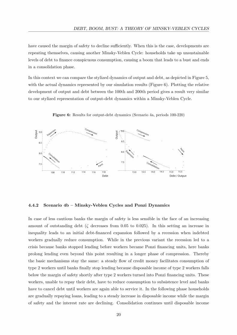
DEBT BOOM BUST A THEORY OF MINSKY-VEBLEN CYCLES
PlotLegend minusgt interest rate LegendPosition minusgt 11 minus04ImageSize minusgt 600]
ListPlot[ Table[listetotdebt[[i]] listey[[i]] i 100 220]PlotStyle minusgt Black ImageSize minusgt 600]
ListPlot[ Table[listedebttogdp[[i]] listey[[i]] i 100 220]PlotStyle minusgt Black ImageSize minusgt 600]
33