Debt as a source of financial stress in Australian households

ANDREW C WORTHINGTON† School of Economics and Finance, Queensland University of Technology, Australia

Abstract This paper examines the role of demographic, socioeconomic and debt portfolio characteristics as contributors to financial stress in Australian households. The data is drawn from the most-recent Household Expenditure Survey Confidentialised Unit Record Files (CURF) and relate to 3,268 probability-weighted households. Financial stress is defined, amongst other things, in terms of financial reasons for being unable to have a holiday, have meals with family and friends, and engage in hobbies and other leisure activities and overall financial management. Characteristics examined included family structure and composition, source and level of household income, age, sex and marital status, ethic background, housing value, debt repayments and credit card usage. Binary logit models are used to identify the source and magnitude of factors associated with financial stress. The evidence provided suggests that financial stress is higher in families with more children or other dependents and from ethnic minorities, especially those more reliant on government pensions and benefits, and negatively related to disposable income and housing value. There is little evidence to suggest that Australia’s historically high levels of household debt are currently the cause of significant amounts of financial stress in these households.

Keywords: Household and consumer debt, owner-occupied and investor housing, financial stress.

JEL classification: C25, D12, G18, R20

Introduction

Household debt has grown dramatically relative to disposable income over recent years, as

has concern that this level of debt poses a threat to the health of global economies. In the

United States mortgage debt and consumer credit relative to disposable income are at or near

all time record highs, with the primary driver being mortgage debt – rising from less than 36

percent of disposable income to more than 66 percent in the last thirty years (Maki 2000).

Since consumer spending accounts for some two-thirds of US GDP, and given that a high

level of indebtedness among households could lead to increased delinquencies and

bankruptcies, and thereby threaten the health of lenders exposed to loan losses, it is argued

that the US economy is then particularly exposed to macroeconomic shocks, especially during

the current period of economic recovery.

By the same token, in the United Kingdom the Bank of England has called for ‘close

monitoring’ of the growth in unsecured lending – some 19 percent of household debt up from

14 percent a decade ago – and has expressed concern about total household debt – currently

Address for correspondence: Associate Professor Andrew C Worthington, School of Economics and Finance, Queensland University of Technology, GPO Box 2434, Brisbane QLD 4001, Australia. Tel. +61 (0)7 3864 2658, Fax. +61 (0)7 3864 1500, email. a.worthington@qut.edu.au

rising by 13 percent annually – and the possible impact on the banking system if the housing

bubble bursts, particularly in London and the Southeast (Nickell 2003; Scheherazade 2002).

There is special concern for the rise in unsecured debt among vulnerable lower-income and

younger households. A similar picture emerges in other OECD economies with total

household debt to income ratios rising from eighty percent or lower in the early 1980s to at

least 120 percent in the UK, Canada, Germany and the US, more than 130 percent in Japan,

and 180 percent in the Netherlands.

In Australia too there has been unease about the growth of household debt (Macfarlane 2003).

In the decade to December 2002 the ratio of household debt to income rose from a level that

was relatively low by international standards (56 percent) to one that is in the upper range for

comparable economies (125 percent) (Macfarlane 2003). This represents an average annual

growth rate of 13.9 percent over the decade and 14.7 percent in the past five years. And while

borrowing for owner-occupied housing still accounts for the major portion of this debt (85.5

percent) and much of its growth (15.3 percent in the last decade and 15.4 percent in the past

five years), substantially faster growth rates are found in borrowing for investor housing (21.6

percent over the decade and 20.7 over the past five years) and credit cards (17.4 percent over

the decade and 20.9 percent in the past five years) (RBA 2003a).

Reasons for the rapid growth in Australian household indebtedness are not hard to find.

Lower mortgage interest rates (averaging 15 percent in the 1980s and 7 percent in the late

1990s) and the fall in servicing costs by itself can account for an almost doubling of

household borrowing. This is particularly the case when combined with the strong and

sustained growth in housing prices, especially in the capital cities (56.9 percent across

Australia and up to 89.3 percent in Melbourne and 62.0 percent in Brisbane from 1997-2002)

(RBA 2002b). At the same time, the low inflation environment of the late 1990s and early

2000s (averaging 2.6 percent), while necessary for the lower interest rate, has its own effect in

that nominal income growth erodes the real value of debt less rapidly than in a high inflation

environment.

Financial deregulation has also had a role to play. To start with, the increase in competition

has meant that the reduction in lending margins of about 2 percent has been fully passed on to

consumers. Similarly, loans for investor housing have risen dramatically as financial

institutions have sought to expand their portfolios with loans on high-return, low-risk

domestic properties, and by offering products with investors in mind such as split-purpose and

interest only loans and deposit bonds (RBA 2002a). Finally, the development of new

products, particularly home-equity loans and redraw facilities, has enabled households to

more flexibly manage equity for building extensions and alterations and other investment and

consumption purposes (RBA 2003b). For example, around 20 percent of borrowers

refinancing home loans over the period 1997-99 used at least some of the proceeds to fund

purchases such as cars and holidays (RBA 2003b).

Nevertheless, it is thought that these outwardly sound contributors to the growth in household

debt obscure some changes that have increased its risk and thereby the exposure of Australian

households to financial stress and the Australian economy to macroeconomic shocks. To start

with, much of the growth in total household debt can be attributed to the very strong growth

of borrowing for investor housing. Because such borrowing is inherently riskier, and given its

high exposure to inner city, multi-unit apartment markets with the immediate prospects of a

glut in supply, it is argued that this exposes some households to a greater level of financial

stress than is the case with purely owner-occupied housing. Next, while aggregate debt

servicing (ratio of interest payments to disposable income) has fallen, households have

increased borrowing by proportionately more than the reduction in interest rates. As with

aggregate gearing (the ratio of the value of housing debt to the stock of housing assets) this at

first appears to have only increased modestly in the past five years, but since most Australian

households hold no housing debt (about seventy percent own their home outright or rent) the

effects are more pronounced than at first suggested (20 percent in across all households but 43

percent in mortgaged households). This suggests that at least some Australian households

may be exposed to a degree of financial stress because of their borrowing. Unfortunately, the

economic and sociological impact of this historically high level of indebtedness is not yet

quantified. That is, it is not known whether Australian households currently experience high

levels of financial stress because of this debt, nor whether it has the potential to expose

households to such stress given an economic shock as feared by many policymakers.

The purpose of the present paper is to add to the small but evolving consumer debt literature

an analysis of financial stress in Australian households using the unit record files underlying

the Australian Bureau of Statistics’ (2002) Household Expenditure Survey. This survey

focuses on the demographic, socioeconomic and financial characteristics of households and

can be linked with these households’ perceptions regarding financial stress, as variously

measured. It thereby provides an important input into current economic policy regarding the

impact of household debt on financial stress as compared to non-debt related influences. To

the author’s knowledge this is the first study of its kind, both in Australia and overseas, and

adds significantly to the literature concerning the psychological impact of consumer debt. The

paper itself is divided into four main areas. The first section briefly reviews the extant

literature regarding consumer debt and household behaviour. The second section explains the

empirical methodology and data employed in the analysis. The third section discusses the

results. The paper ends with some brief concluding remarks.

Literature review

In contrast to the voluminous literature concerned with corporate debt, hypotheses to explain

the causes and consequences of household debt are relatively underdeveloped. Most studies

are conducted at the aggregate level, and it is only comparatively recently that efforts have

been made to construct a conceptual, theoretical and empirical body of work analogous to that

concerning the corporate sector. The literature that does exist may be categorised into three

main areas: (i) attempts to explain differing household financial strategies, or the different

patterns of financial assets and debts found in households, and link these with consumption,

saving and borrowing behaviour; (ii) efforts to investigate the factors which are associated

with the source, level and conditions of debt which a household demands and is granted or

rejected; and (iii) endeavours which explore the issues related to insolvency in household

finances, usually in terms of predictive models of debt repayments, delinquency and

bankruptcy.

To start with, a small amount of empirical attention has been directed at analysing the linkage

between household portfolio choices and other household behaviour. This is important

because the impact of policies on households’ saving and debt behaviour (and consumption)

can vary across different groups in an economy in ways not reflected at the aggregate level.

Gunnarsson and Wahlund (1997), for example, categorised the financial choices of one

thousand Swedish households into residual saving, contractual saving, security saving, risk

hedging, prudent investing and ‘divergent’ strategies and examined the impact of financial

planning and control, financial wealth and home ownership, and attitudes to risk taking across

these categories. For debt, Gunnarssosn and Wahlund (1997) concluded that contractual

savers had a very heavy debt burden and relied upon credit cards, whereas residual savers had

fewer loans and few even possessed credit cards. Alternatively, Viaud and Roland-Levey

(2000) organised a typology of four classes defined along the lines of how households strived

to build up their capital: namely, ‘accumulating savers’, ‘prodigal households’, ‘prudent

agents’ and ‘fragile borrowers’. Using the concept of social identity Viaud and Roland-Levey

(2000) reasoned why households in different economic positions may in fact have the same

structural relationships regarding savings and credit.

Other work in this area has generally concentrated on the link between household portfolios

and decisions regarding consumption or savings/borrowing. For example, de Ruiter and

Smant (1999) examined the relationship between the household balance sheet and consumer

durables expenditure. In particular, they addressed the potential impact of the excessive debt

burdens built up by households and financial deregulation in the 1980s and questioned if it

might be behind the slow recovery of OECD economies. While finding, not entirely

unexpectedly, that household wealth was an important determinant of consumer expenditure;

they found no evidence that the ‘excessive’ household debt ratios of the 1980s were directly

responsible for slowing down consumer durables expenditure during the period of economic

recovery. Moreover, DeRuiter and Smant (1999: 266) concluded that an emphasis on debt-

income ratios at the aggregate level was misleading and that it was “…probably merely an

illustration of common failures to consolidate balance sheets on an appropriate level when

discussing macroeconomic issues”. Lastly, Engelhardt (1996) examined the empirical link

between house price appreciation and the saving/borrowing behaviour of homeowners during

the 1980s. Interestingly, it was concluded that a savings asymmetry existed in that households

that experience real gains in wealth do not change their saving/borrowing behaviour, rather all

the savings offset was from households that experienced a real capital loss.

The second and generally more extensive area of empirical research focuses on the demand

for household debt. At least some part of this work is aimed at differentiating mortgage

demand and housing demand, while others are concerned with the interactions between the

choice of mortgage instrument and the role of mortgage rationing and liquidity constraints.

Leece (2000a), for instance, used the UK Family Expenditure Survey to estimate reduced

form mortgage demand equations to analyse the impact of market rationing and financial

liberalisation on households. The main findings of this analysis were that there is significant

cross-sectional variation regarding the demand for mortgages and that the choice of mortgage

instrument involving saving in an alternative investment vehicle reflects important portfolio

and liquidity consideration (Leece 2000b). Leece (2000b) also examined the determinants of

UK household mortgage debt, though using the British Household Panel Survey and in the

context of the choice between floating or fixed interest rates. Leece (2000b) concluded that no

socioeconomic variables, including age and first-time buyers and marital status, were

significant factors in influencing this choice of mortgage instrument.

Demand functions for household debt have also been modelled in the United States. For

example, using the Survey of Consumer Finance Crook (2001) examined the factors that

determined whether a credit applicant was likely to be rejected and/or discouraged from future

application and what variables significantly affected the demand for household debt. While it

was concluded that household debt was a function of household age, income, size and

employment status, it was largely invariant to the level of expected future interest rates.

Alternatively, Ling and McGill (1998) used the American Housing Survey to simultaneously

estimate mortgage debt level with house value. Ling and McGill (1998) concluded that larger

debt values were often associated with greater value residences and with the level of

household income, along with household mobility and other demographic variables.

Breuckner (1994, 1997), Jones (1993, 1994, 1995), Hendershott et al. (1997) and Lea et al

(1993, 1995) have also examined the demand for household debt as a function of financial,

demographic and socioeconomic factors.

The final area of empirical research is concerned with consumer debt repayment in the

context of household insolvency, delinquency and bankruptcy. Böheim and Taylor (1998), for

example, examined evictions and repossessions using the British Household Panel Survey.

The results showed that previous experience of financial problems had a significant and

positive association with the current financial situation and the probability of eviction, and

that negative financial surprises were an important route into financial difficulties after

controlling for life events such as divorce and loss of employment. Walker (1996) also

examined a significant life event (childbirth) as source of financial strain and presented

evidence that psychological and behavioural variables had a considerable impact on being in

or keeping out of debt. Canner and Luckett (1990), DeVaney and Lytton (1995), DeVaney

(1994), Domowitz and Sartain (1999), Gropp et al. (1997), Kau and Keenan (1999),

Muelbauer and Cameron (1997) also analysed debt in the context of household repayment

difficulties, insolvency and bankruptcy.

This rather more sizeable area of empirical inquiry is generally consistent with DeVany and

Lytton’s (1995) survey evidence that many demographic and socioeconomic variables

influence household debt repayment, the likelihood of default, the propensity for insolvency

and ultimately bankruptcy. For example, renter and ethnic minority status, level of education

and households with higher ratios of mortgage or consumer debt payments to income are

often significant determinants of missed or slow debt payments. Similarly, DeVany and

Hanna (1995) found that the age and income of the household head had a negative

relationship with the propensity for insolvency, as did married couples. Alternatively, Lunt

and Livingstone (1992) concluded that socio-demographic variables such as social class, age

or the number of dependent children were not significant predictors of car debt repayment,

though not so disposable income.

When examining existing research on household debt, a number of salient points emerge.

First, almost all of this work has been undertaken in the United States and, to a lesser extent,

the United Kingdom. Relatively little attention has been paid to disaggregated sets outside of

these financial milieus, not least in Australia. Second, there has been an overwhelming

emphasis in studies examining problems associated with household debt to focus on extreme

conditions such as insolvency and bankruptcy. Certainly, it is expected that households with

potential repayment problems would experience less severe examples of financial stress long

before these events take place, including cutting back on discretionary areas of consumption,

and these are therefore suggestive of leading indicators of debt repayment problems. Finally,

much of the existing literature pre-dates the increase in household debt levels found in the

past five years. This is important because the full impact of sustained low interest rates and

inflation and financial deregulation are only now being fully felt. That is, guidance could be

had on the degree of financial stress that exists when debt service and gearing are at historical

highs. It is with these considerations in mind that the present study is undertaken.

Research method and data

All data is obtained from the Australian Bureau of Statistics’ (ABS) (2002) Household

Expenditure Survey Confidentialised Unit Record File (CURF) and relate to a sample of 3,268

probability-weighted Australian households with at least some outstanding debt. The strength

of this data is that it is a national survey concerning the demographic, socioeconomic and

financial characteristics of Australian households and for the first time includes a number of

items to identify financial stress in households. Unfortunately, it comprises a single cross-

section so there is no meaningful way in which household behaviour in the most recent survey

can be linked with the results of earlier surveys and many of the categories of income and

expenditure can only be interpreted realistically at the household, as against the personal,

level.

The analytical technique employed in the present study is to specify households’ perceptions

of financial stress as the dependent variable (y) in a regression with demographic,

socioeconomic and debt characteristics as explanatory variables (x). The nature of the

dependent variable (either no financial stress or financial stress) indicates discrete dependent

variable techniques are appropriate. Accordingly, the following binary logit model is

specified:

xβey ′−+

==1

1)1(Prob (1)

where x comprises a set of characteristics posited to influence the presence of financial stress,

β is a set of parameters to be estimated and e is the exponential. The coefficients imputed by

the binary logit model provide inferences about the effects of the explanatory variables on the

probability of financial stress.

The dataset employed is composed of four sets of information. All of the sets are derived

from the survey responses. The first set of information relates to several different dimensions

of financial stress and comprises the dependent variable in the binary logit model specified in

equation (1). In the survey the respondents were asked whether their present standard of

living was worse than two years ago (STD), indicate whether it was for financial reasons that

they did not have a holiday away for a least one week a year (HOL), have a night out once a

fortnight (NTO), have friends or family over for a meal once a month (FML), have a special

meal once a week (SPM), buy second-hand clothes most of the time (CLH) and do not spend

time on leisure or hobby activities (HOB), and whether they spend more money than they get

most weeks (MGT) (y = 1). For STD the control was that the household living standard was

better or the same as two years ago, for HOL, NTO, FML, SPM, CLH and HOB that the

household either engaged in the stated activity or did not because of non-financial reasons

only, and for MGT that the household broke even or saved money most weeks (y = 0). These

eight binary variables comprise the dependent variables in eight separate analyses aimed at

explaining the causes of financial stress in Australian households.

Selected descriptive statistics are provided in Table 1. Overall, 758 households (23.19

percent) believed their standard of living was worse than two years earlier, 914 (27.97

percent) could not afford a holiday for one week a year, 665 (20.35 percent) could not afford a

night out once a fortnight, 140 (4.25 percent) could not afford to have friends or family over

for a meal once a month, 347 (10.47 percent) could not afford a special meal once a week,

317 (9.70 percent) could not afford to buy brand new clothes most of the time and 278 (8.51

percent) could not afford to spend time on leisure or hobby activities. In terms of financial

management, 2,204 households or 67.44 percent stated that the household usually spent more

money than it received, as against breaking even or saving money most weeks. The internal

reliability of these eight measures is relatively high (α=0.7299) suggesting broad agreement

between the alternative dimensions of financial stress.

<TABLE 1 HERE>

The next three sets of information are specified as explanatory variables in the binary logit

regression models. The first of these sets of information relates to household demographic

characteristics, the second to socioeconomic characteristics, and the final set to debt

characteristics. The first two sets of information are generally comparable to those employed

in studies of household debt repayment, insolvency and bankruptcy and are intended to proxy

for the factors thought to be non-debt sources of financial stress. The third set of information

is used to identify households with different levels of debt service as a means of establishing a

connection with household financial stress beyond these factors.

The set of demographic variables upon which the financial stress indicators are regressed are

first examined. Whilst there is no unequivocal rationale for predicting the direction and

statistical significance of many of these independent variables, their inclusion is consistent

with both past studies of the determinants of household financial stress (as variously defined)

and the presumed interests of policy-makers and other parties. For example, Böheim and

Taylor (2000) used personal characteristics and demographics of the household head to help

determine the level of transaction costs, preferences and attitudes to risk, and household

structure concerning the number and ages of children as explanatory variables in their study

of evictions and repossessions, while Ling and McGill (1998) included ethnic background as

a means of controlling for variation in household risk preferences.

The first six variables relate to household structure. These represent households composed

respectively of couples and lone parents with children over 15 years of age (CPO and LPO),

couples and lone parents with children 14 years or younger (CPY and LPY) and couples and

lone parents with children both under 14 years and over 15 years (CPB and LPB). The control

for these variables is single person or couple only households. The next eleven variables

relate to the sex, age, marital status and ethnic background of the household head. These are

used as proxies for general characteristics including stage of life cycle, unobservable risk

preferences and access to labour and credit markets. For instance, Böheim and Taylor (2000)

reasoned non-whites may have experience difficulties with debt payments because of a lack of

familiarity with financial institutions or the differential access to credit, while Canner and

Luckett (1991) found in a study of US households that divorced or separated and younger

persons were more likely to experience debt repayment problems, as did DeVaney and Hanna

(1994). The variables specified include the sex (SEX), age (AGE) and marital status of the

household head (DIV and MAR), whether the household head was born in Oceania (OCE),

Europe (EUR), the Middle East and North Africa (MID), Asia (ASA), the Americas (AMR) or

Sub-Saharan Africa (AFR) and the year of arrival in Australia (RES). The control variables for

SEX, DIV and MAR and OCE, EUR, MID, ASA, AMR and AFR are male, unmarried and born

in Australia household heads, respectively. The final two variables are included to reflect

additional dimensions of household structure and characteristics. These are the number of

income units (INU) and the number of dependents (DEP) in each household. Ling and McGill

(1998), for example, identified two-wage earning households as a positive indicator of

financial strain along with the number of children.

The next group of variables relate to the income characteristics of each household. The first

three variables are dummy variables indicating whether the principal source of household

income is derived from self-employment (SEL), superannuation and investments (SUP) or

government pensions and benefits (BEN). The control is wages and salaries as the principal

source of household income. In this instance, and holding income constant, it is hypothesised

that the more fixed the level of permanent income and the lower the ability to earn extra

income, the higher the level of financial stress. Böheim and Taylor (2000) likewise

hypothesised that sources of income were a potential source of financial stress in that a

household with a retired head was more likely to report housing finance difficulties than

employees, and observing that in many cases self-employment predated indebtedness because

of the interaction between businesses and the collateral provided by housing wealth.

The next two variables indicate whether the principal residence is being bought (MRT) or

rented (RNT) (control is owned outright) (Canner and Luckett 1991). It is generally the case

that transaction costs associated with owner-occupation are sizeable when compared to

renting, while mortgaged households with large fixed payments and a general lack of mobility

may be less able to adjust to changes in regional employment conditions. Lastly, the estimated

value of the principal dwelling (VAL) and the level of household disposable income (DIC) are

also included. All other things being equal, greater wealth and/or income should expose debt

holders to a lower level of financial stress.

By and large, the distributional properties of the demographic and socioeconomic variables

appear non-normal. Most of the values, with the exception of MAR and MRT are positively

skewed, indicating a long right tail for the continuous variables and the much lower

probability of ones as against zeros in the binary variables. Since the asymptotic sampling

distribution of skewness is normal with mean 0 and standard deviation of T6 , where T is

the sample size, then the standard error under the null hypothesis of normality is 0.0428: all

estimates of skewness are then significant at the .10 level or higher. The kurtosis, or degree of

excess, in most variables is also generally positive and larger than three, ranging from 4.1359

for CPO to 104.1036 for AFR, thereby indicating leptokurtic or peaked distributions. The

kurtosis for DIV, EUR, AGE, DEP, RNT, MAR, CPY, SEX and MRT is significantly less than

three indicating relatively flat or platykurtic distributions [the sampling distribution of

kurtosis is normal with mean 3 and standard deviation of 0856.024 =T ]. Finally, Jarque-

Bera statistics and p-values (not shown) are used to test the null hypotheses that the

distribution of these variables is not normally distributed. All p-values are smaller than the .01

level of significance suggesting the null hypothesis can be rejected.

The final eight variables in Table 1 represent the indebtedness of households. The six debt

service ratios used are calculated by dividing the weekly repayments (in dollars) for various

categories of loans by disposable income. The categories examined are loans to buy or build

this (RBP) or other property (ROP), loans for alternations and additions to this (RAL) or other

property (ROL) and loans for motor vehicles (RMV), holidays (RHL) and other purposes

(ROT). Broadly, RBP and RAL are loans for owner-occupied housing while ROP and ROL are

loans for investor housing, though there may be some interplay between these and loans for

other purposes due to the existence of equity loans and redraw facilities. A measure of

personal debt is also included in the form of the number of household credit cards, which in

the absence of available credit limit, is the closest approximation of credit card debt available.

On average, loans to buy and build owner-occupied housing account for 34.52 percent of

disposable income, loans for investor housing 4.47 percent, owner occupied and investor

housing alterations and additions 0.67 and 0.22 percent respectively, and loans for motor

vehicle, holidays and other purposes 6.06, 0.12 and 1.66 percent respectively. The average

household also has 1.44 credit cards.

Tests for differences in means and proportions for the explanatory variables in Table 2

indicate statistically significant differences between households that do not and do experience

financial stress across a number of the categories. For example, and all other things being

equal, households seeing their standard of living as being worse than two years previously

(STD) are more likely to be couples with children both under 14 and over 15 years (CPB),

lone parents with children 14 years and younger (LPY) and 15 and over (LPO), with a female

(SEX), older (AGE), divorced or separated (DIV) householder, with superannuation and

investments (SUP) or government pensions and benefits (BEN) as the primary source of

income and with a lower value of residence (VAL) and disposable income (DIC). These

households are also likely to have a higher level of repayments relative to disposable income

for loans for other purposes (ROT) and fewer credit cards (CRC).

<TABLE 2 HERE>

Households that indicate that they spend more money than they get most weeks (MGT) are

significantly more likely to be drawn from couples with younger children (CPY) and both

younger and older children (CPB), all categories of lone parents (LPY, LPO, LPB),

households with female (SEX), divorced/separated (DIV) and born in North Africa and the

Middle East (MID) heads, depending on government pensions and benefits (BEN) and a larger

number of dependents (DEP). They are also more likely to be renting (RNT) and pay a higher

debt-service ratio on other loans (ROP) and with lower residential housing value (VAL) and

disposable income (DIC) and a smaller number of credit cards (CRC). Overall, there are

significant differences in demographic, income and debt characteristics between household

that do and do not experience financial stress across one hundred and forty-two of the two

hundred and seventy-two factors (52.2 percent). However, only twenty significant differences

in financial stress are found across the sixty-four dimensions of debt (31.25 percent) of which

nearly all are concerned with repayments on loans for other purposes (ROT) or the number of

credit cards (CRC).

Empirical findings

The estimated coefficients, standard errors and p-values of the parameters for the logit

regressions are provided in Table 3. To facilitate comparability, marginal effects are also

calculated. These indicate the marginal effect of each outcome on the probability of

experiencing financial stress. Also included in Table 3 are statistics for the log-likelihood (L),

restricted slopes log-likelihood (RL), likelihood ratio (LR) tests, the McFadden R2 as an

analogue for that used in the linear regression model and the Hannan-Quinn Criterion (HC) as

a guide to model selection. Sixteen separate models are estimated. The estimated coefficients,

standard errors, p-values and marginal effects employing the entire set of demographic,

socioeconomic and debt characteristics as predictors for the eight measures of financial stress

are presented initially, followed by a refined specification for each of these measures obtained

using forward stepwise regression using the Wald criteria.

In all cases, and as indicated by the lower values of HC, the refined models are to be preferred

over the beginning specifications in terms of the trade-off between comprehensiveness and

complexity. Yet irrespective of specification, all of the estimated models are highly

significant, with likelihood ratio tests of the hypotheses that all of the slope coefficients are

zero rejected at the 1 percent level or lower using the likelihood ratio statistic. The results in

these models also appear sensible in terms of both the precision of the estimates and the signs

on the coefficients. To test for multicollinearity, variance inflation factors (VIF) are calculated

and presented in Table 1. As a rule of thumb, a VIF greater than ten indicates the presence of

harmful collinearity. Amongst the explanatory variables the highest VIFs are for RES

(3.3449), CPY (3.0625), and RNT (3.009). This suggests that multicollinearity, while present,

is not too much of a problem.

<TABLE 3 HERE>

The first model discussed is that predicting financial stress by comparing the current standard

of living with those two years previously (STD). In the beginning model, the estimated

coefficients for CPO, CPB, LPO, DIV, MID, RES, INU, DEP, BEN and DIC are significant at

the 10 percent level of significance or lower and conform to a priori expectations. The

estimated coefficients in the beginning specification thus indicate that couples with children

fifteen years and over with and without younger children, lone parents with older children,

divorced or separated household heads, recently arrived household heads born in North Africa

and the Middle East, households with a higher number of dependents and income units and

those on government pensions and benefits and lower disposable incomes are more likely to

indicate that their present standard of living is worse than two years earlier. The three greatest

influences on this viewpoint (marginal effect in brackets) is being from a North African or

Middle Eastern background (MID) (3.1530), and being a couple with both younger and older

children (CPB) (1.8187) or on government pensions and benefits (BEN) (1.5588).

These results are generally consistent with the estimated coefficients in the refined model,

which is obtained by forward stepwise regression using a Wald criterion. Seven variables

(excluding the constant) are stepped into the model on this basis (W-statistics and p-values in

brackets): DIC (78.27, 0.0000), INU (21.93, 0.0000), AGE (8.45, 0.0040), DEP (6.95,

0.0080), BEN (6.84, 0.0090), MID (6.49, 0.0110) and CPB (4.13, 0.0420). All of these factors

are associated with increasing levels of financial stress with the exception of disposable

income, which is negatively reacted to financial stress. Interestingly, none of the parameters

associated with household debt are significant, suggesting that demographic and, to a lesser

extent, socioeconomic influences dominate perceptions of increasing financial stress.

Broad agreement is found with the estimated coefficients and signs on the estimated

coefficients in the next six refined models where HOL, NTO, FML, SPM, CLH and HOB are

specified as the dependent variables. In all of these regressions, financial stress is negatively

associated with the value of the dwelling (VAL) and disposable income (DIC) and positively

associated with the number of income units (INU) and dependents (DEP), whether the

principal source of household income is from government pensions and benefits (BEN) and

whether the household head is born in North Africa or the Middle East (MID). The remaining

significant factors (with dependent variable) are LPO, LPY, RES and CRC (HOL), AGE,

MAR, SEL and MRT (NTO), LPB and ASA (FML), CRC (CLH) and LPY, SEL and CRC

(HOB). With the exception of the number of credit cards (CRC) and whether the principal

source of household income is from self-employment (SEL) all of the signs on the estimated

coefficients are positive.

The results in the final two regressions in Table 3 are where financial stress in overall

household management (defined as spending more money than received most weeks) is

regressed against the same set of explanatory variables. In the beginning model the

coefficients for couples with both older and younger children (CPB), female-headed (SEX)

and married or de facto (MAR) households, recently arrived (RES) household heads from a

North African or Middle Eastern background (MID), the number of income units (INU) and

dependents (DEP), households on government pensions and benefits (BEN), renting

households (RNT), households with lower disposable incomes (DIC) and higher repayments

for loans for other purposes (ROT) are significant at the .10 level or lower and the signs on

these coefficients are consistent with a priori expectations. A refined model based on forward

stepwise regression includes seven variables (excluding the constant) in the order of (W-

statistics and p-values in brackets): DIC (174.47, 0.0000), DEP (124.56, 0.0000), INU (77.99,

0.0000), BEN (9.21, 0.0024), ROT (7.04, 0.0080), RNT (6.51, 0.0107) and RBP (2.57,

0.1089). Overall, households with more income earning units, a larger number of dependents,

those that rely principally on government pensions and benefits, renting and lower disposable

income households, those with lower repayments on loans for buying and building owner-

occupied housing and higher repayments on loans for other purposes are more likely to spend

more money than is received most weeks. The greatest marginal effects on this form of

financial stress are high repayments on loans for other purposes, households with larger

number of income units and those dependent upon government pensions and benefits as the

principal source of income.

At first impression, it would appear that debt has little role to play in determining financial

stress in Australian households. In fact, only for household management (MGT) is the

repayment of a loan (ROT) both significant and conform to its hypothesised sign, while the

number of credit cards even where significant (HOL, CLH and HOB) is negative suggesting a

contradiction with a priori reasoning. In the case of the latter, it is of course likely that better

access to credit cards increases financial flexibility and therefore has a role in diminishing

financial stress in all but the most extreme circumstances. For the former, redundant variable

tests of RBP, ROP, RAL, ROL, RMV, RHL and ROT reject the null hypothesis of joint

insignificance (F-statistics and p-values in brackets) for HOL (3.99, 0.0000), SPM (1.93,

0.0514), CLH (5.77, 0.0000), HOB (5.72, 0.0000) and MGT (2.28, 0.0194). This suggests that

debt portfolios exert a weak but significant influence on financial stress, but this is offset by

effects elsewhere. A real possibility is that households are currently willing to carry high

levels of debt with little financial stress seemingly confident that the capital gains provided by

strong owner-occupied and investor housing markets, access to equity loans and other

household investments, and a low and stable outlook for inflation and mortgage interest rates

will provide financial flexibility for the foreseeable future.

As a final requirement, the ability of the various models to accurately predict outcomes in

terms of financial stress is examined. Table 4 provides the predicted results for each refined

model and compares these to the probabilities obtained from a constant probability model.

The probabilities in the constant probability model are the values computed from estimating a

model that includes only an intercept term, and thereby correspond to the probability of

correctly identifying financial stress on the basis of the proportion experiencing it in the

sample. To start with, consider the model where HOL (a holiday away for at least one week a

year) is specified as the dependent variable. Of the 3,268 households in the sample, 2,354

either had such a holiday or did not for some non-financial reason and 914 indicated that they

could not afford such a holiday. Of these the constant probability model correctly predicts

1,696 cases (72.03 percent) as having ‘no financial stress’ and 256 cases (27.97 percent) as

having financial stresses. This represents the correct prediction of 1,952 cases (or 59.71

percent) of all households. By way of contrast, the refined model correctly identifies 2,209

cases (93.84 percent) as not having financial stress and 249 cases (27.24 percent) as having

financial stress. Thus, the model correctly identifies 2,458 of the 3,268 households (or 75.21

percent) in terms of financial stress or not. This indicates an absolute improvement of 25.92

percent over the constant probability model (in terms of the number of correct predictions)

and a relative improvement of 38.40 percent (in terms of the number of incorrect predictions).

<TABLE 4 HERE>

The refined model for the remaining seven dimensions of financial stress delivers a

comparable level of correct and incorrect predictions. The total percentages of correct

prediction across these models (percentage of correct predictions for constant probability

models in brackets) are: STD 77.05 (64.37), NTO 79.83 (67.58), FML 95.62 (91.86), SPM

89.32 (81.26), CLH 90.33 (82.48), HOB 91.40 (84.43) and MGT 71.30 (56.08). Of course,

these are ‘in-sample’ predictions and the results could differ if ‘out-of-sample’ data was made

available. It can be seen is that there is little relative improvement between the constant

probability and refined models for FML and SPM and an obvious factor is the very small

proportion of households who do not undertake these most basic of social activities because

of financial hardship. Likewise, the models generally do much better in predicting the absence

of financial stress, and this is not necessarily the most natural focus of interest. For example,

just 1.08 and 1.46 percent of financially stressed households are predicted correctly when the

dependent variable is respectively HOB and SPM, though 91.52 percent of financially

stressed households are predicted correctly when MGT is specified as the dependent variable.

Regardless, Hosmer-Lemeshow goodness-of-fit test statistics for all the models with the

exception of NTO fail to reject the null hypotheses of no functional misspecification and we

may conclude that the models are appropriate for predicting financial stress in Australian

households.

Concluding remarks and policy recommendations

The present study uses binary logit models to investigate the role of demographic,

socioeconomic and debt characteristics in determining financial stress in Australian

households. The current paper extends empirical work in this area in at least two ways. First,

it represents the first attempt using qualitative statistical techniques to model financial stress

in Australian households. This provides an important starting point for future research in this

area. Second, rather than focusing on progressively more acute life events such as problems

with debt repayment, insolvency and bankruptcy as found in previous empirical work, this

study examines financial stress as defined by the inability to engage in commonplace social

functions and family leisure activities. No comparable study is then thought to exist elsewhere

with a focus on financial stress at the margin rather than at the extreme. The evidence

provided suggests that financial stress is very much a function of the demographic and

socioeconomic characteristics of households and, to a lesser extent, debt portfolios.

First, it has been shown that the primary causes of financial stress in Australian households

are basic demographic characteristics. These include the presence of children, the number of

dependents and income-earning units, the age of the household head, and also whether the

householder was born and a recent immigrant from North Africa and the Middle East and, on

occasion, Asia. Policies already in place such as governmental assistance with child support

and childcare stand out, especially since being a lone parent is two to three times more likely

to suffer financial stress than a couple in the same situation, but the underlying cause of

financial stress in Middle Eastern households especially is unknown. One possibility is a

general lack of financial literacy skills and management; another is the interplay of global

political events and higher perceived risk in, say, labour and credit markets. Regardless of

source, such impacts are significant with Middle Eastern households anywhere from two to

four times more likely to suffer financial stress in a given situation. Second, it has also been

shown that household socioeconomic factors also have a role in fostering financial stress. Key

factors here include the increase in financial stress when a household is dependent upon

government pensions and benefits and the decrease in financial stress associated with higher

values of owner-occupied housing and disposable income. By itself, a ten percent fall in

housing values could be associated with up to an eight percent increase in the likelihood of

being financial stressed, depending on the dimension employed. This is important because the

prospective collapse of both the owner-occupied and investor property markets is feared for

its potential impact on aggregate consumption and thereby macroeconomic stability.

Finally, the results indicate that, for the most part, the historically high levels of indebtedness

by Australian households appear to have little impact at the margin on financial reasons for

being unable to engage in basic social activity such as having family and friends over for

meals, having a night out, going on holiday or engaging in hobbies and other leisure activities.

A key likelihood is that the very strong owner-occupied and investor housing market coupled

with historically (and forecast to continue) low mortgage interest rates provides reassurance to

households taking out debt, which in the main, is focused on housing-related purposes.

Households have also used a variety of other strategies to cope with the growth in

indebtedness including refinancing with lower interest rates, extending the term of housing

loans and substituting mortgage borrowing for more expensive consumer debt (DeKaser

2003). That debt-related financial stress that does exist is not associated with housing, motor

vehicle or holiday debt and thereby relates largely to unsecured debt. That said credit cards

themselves seem to offer much in reducing financial stress for Australian households,

reinforcing the view that they use the flexibility of this form of debt to maintain basic social

and consumption activities.

There are, of course, a number of limitations in this study, all of which suggest further areas

of research. To start with, the results of this analysis are framed around what could be

regarded as relatively mild forms of financial stress; that is, the inability to engage in basic

social activities such as meals with family and friends, nights out, holidays, etc. Certainly,

most work in this area has emphasised the more extreme forms of financial stress, including

insolvency and bankruptcy, and it may be that predictive modelling in that instance could be

relatively more accurate, especially when using the demographic, socioeconomic and

financial characteristics employed in this study. Another possibility is that the current study

has not addressed how households manage financial stress in terms of substituting between

activities or reducing the frequency of these activities. In particular, little is known about how

households use sources of emergency finance to maintain consumption with temporary

changes in income and wealth, even though there is some evidence that this practice, though

unsustainable in the longer term, is increasing. Finally, there is renewed concern in Australia

over the prohibitive costs of owner-occupied housing, especially for young first-home buyers.

In this study age did not appear to be a determining factor of financial stress, though in view

of the life cycle approach to household debt this may not be the case in a subset of younger

households.

References

Athreya, K. B. (2002). Welfare implications of the Bankruptcy Reform Act of 1999, Journal of Monetary Economics, 49(?), 1567-1595

Australian Bureau of Statistics (2002) 1998-99 Household Expenditure Survey Australia, Confidentialised Unit Record File, ABS. Cat. No. 6544.0.30.001

Böheim, R. and Taylor, M. (2000) My home was my castle: Evictions and repossessions in Britain, Journal of Housing Economics, 9(4), 287-319.

Brueckner, J.K. (1994) The demand for mortgage debt: Some basic results, Journal of Housing Economics, 3(1), 1-21.

Brueckner, J.K. (1997) Consumption and investment motives and the portfolio choices of homeowners, Journal of Real Estate Finance and Economics, 15(?), 159-180

Canner, G.B. and Luckett, C.A. Consumer debt repayment woes: Insights from a household survey, Journal of Retail Banking, 12(1), 55-62.

Crook, J. (2001) The demand for household debt in the USA: Evidence from the 1995 Survey of Consumer Finance, Applied Financial Economics, 11(1), 83-91.

DeKaser, R. (2003). Don’t sweat the debt! ABA Banking Journal, 95(4), 72 DeRuiter, M. and Smant, D. J. (1999) The household balance sheet and durable consumer expenditures: An

empirical investigation for The Netherlands, 1972-93, Journal of Policy Modelling, 21(2), 243-274. DeVaney, S. A. and Lytton, R.H. (1995) Household insolvency: A review of household debt repayment,

delinquency and bankruptcy, Financial Services Review, 4(2), 137-156. DeVany, S.A. (1994) The usefulness of financial ratios as predictors of household insolvency: Two perspectives,

Financial Counselling and Planning, 5(1), 5-24. DeVany, S.A. and Hanna, S. (1994) The effect of marital status, income, age and other variables on insolvency

in the USA, Journal of Consumer Studies and Home Economics, 18(?), 293-303. Domowitz, I. and Sartain, R. (1999) Determinants of the consumer bankruptcy decision, Journal of Finance,

54(1), 403-420. Engelhardt, G. V. (1996). House prices and homeowner savings behaviour, Regional Science and Urban

Economics, 26(?), 313-336 Gropp, R., White, M.J. and Scholz, J.K. (1997) Personal bankruptcy and credit supply and demand, Quarterly

Journal of Economics, 112(1), 217-251. Gunnarsson, J. and Wahlund, R. (1997) Household financial strategies in Sweden: An exploratory study, Journal

of Economic Psychology, 18(1), 201-233. Hendershott, P. H., LaFayette, W.C. and Haurin, D.R. (1997) Debt usage and mortgage choice: The FHA-

conventional decision, Journal of Urban Economics, 41(?), 202-217 Jones, L.D. (1993) The demand for home mortgage debt, Journal of Urban Economics, 33(1), 10-28 Jones, L.D. (1994) Home mortgage debt financing of non-housing investments, Journal of Real Estate Finance

and Investment, 9(1), 91-112 Jones, L.D. (1995) Net wealth, marginal tax rates and the demand for home mortgage debt, Regional Science

and Urban Economics, 25(?), 297-322. Kau, J.B., and Keenan, D.C. (1999) Patterns of rational mortgage default, Regional Science and Urban

Economics, 29(?), 765-785. Lea, S.E.G., Webley, P. and Levine, R.M. (1993) The economic psychology of consumer debt, Journal of

Economic Psychology, 14(1), 85-119 Lea, S.E.G., Webley, P. and Levine, R.M. (1995) Psychological factors in consumer debt: Money management,

economic socialisation and credit use, Journal of Economic Psychology, 16(?), 681-701. Leece, D. (2000a) Choice of mortgage instrument, liquidity constraints and the demand for housing debt in the

UK, Applied Economics, 32(?), 1121-1132. Leece, D. (2000b). Household choice of fixed versus floating rate debt: a binomial probit model with correction

for classification error, Oxford Bulletin of Economics and Statistics, 62(1), 61-82. Ling, D. C. and McGill, G. A. (1998) Evidence on the demand for mortgage debt by owner-occupants, Journal

of Urban Economics, 44(3), 391-414 Lunt, P. and Livingstone, S. (1992) Predicting personal debt and debt repayment: Psychological, social and

economic determinants, Journal of Economic Psychology, 13(1), 111-134. Maki, D. M. (2000) The growth of consumer credit and the household debt service burden, Board of Governors

of the Federal Reserve System Working Paper, No. 2000/12. McFarlane, I.J. (2003) Do Australian households borrow too much? <http://www.rba.gov.au/>, Accessed July

2003. Muelbauer, J. and Canmeron, G. (1997) A regional analysis of mortgage possessions: Causes, trends and future

prospects, Housing Finance, 34(1), 25-34. Nickell, S. (2003) House prices, household debt and monetary policy, Bank of England Quarterly Bulletin,

43(1), 131-136. Reserve Bank of Australia (2002a) Innovations in the provision of finance for investor housing, Reserve Bank of

Australia Bulletin, December, 1- 6

Reserve Bank of Australia (2002b) Recent developments in housing: Prices, finance and investor attitudes, Reserve Bank of Australia Bulletin, July, 1-6.

Reserve Bank of Australia (2003a) Household debt: What the data show, Reserve Bank of Australia Bulletin, March, 1-11.

Reserve Bank of Australia (2003b) Housing equity withdrawal, Reserve Bank of Australia Bulletin, February, 50-54

Scheherazade, D. (2002). Consumer debt rising and worsening, warns bank: Financial stability review alarm over house buyers’ borrowing and spiralling debt among vulnerable groups, Financial Times, 12 December, 3.

Stango, V. (1999) The Tax Reform Act of 1986 and the composition of consumer debt, National Tax Journal, 52(4), 717-739

Stevens, G.R. (1997) Some observations on low inflation and household finances, Reserve Bank of Australia Bulletin, October, 38-47

Viaud, J. and Roland-Levy, C. (2000) A positional and representational analysis of consumption: Households when facing debt and credit, Journal of Economic Psychology, 21(?), 411-432.

Walker, C. M. (1996) Financial management, coping and debt in households under financial strain, Journal of Economic Psychology, 17(?), 789-807

TABLE 1. Dependent and independent variable definitions and descriptive statistics

Variable description Mean Std. dev. Skewness Kurtosis VIF Present standard of living compared with two years ago STD 0.2319 0.4221 1.2708 -0.3854 – Reason household does not have a holiday away at least one week a year HOL 0.2797 0.4489 0.9822 -1.0360 – Reason household does not have a night out once a fortnight NTO 0.2035 0.4027 1.4737 0.1719 – Reason household does not have friends or family over for a meal once a month FML 0.0425 0.2018 4.5359 18.5855 – Reason household does not have a special meal once a week SPM 0.1047 0.3062 2.5843 4.6814 – Reason household buys second hand clothes most of the time CLH 0.0970 0.2960 2.7246 5.4267 – Reason household does not spend time on leisure or hobby activities HOB 0.0851 0.2790 2.9760 6.8607 – Overall management of household income MGT 0.6744 0.4687 -0.7448 -1.4462 – Couple with children over 15 years of age CPO 0.1111 0.3143 2.4766 4.1359 1.6267Couple with children 14 years or younger CPY 0.3081 0.4618 0.8314 -1.3095 3.0625Couple with children both under 14 years and over 15 years CPB 0.0737 0.2614 3.2634 8.6549 1.9420Lone parent with children over 15 years of age LPO 0.0321 0.1764 5.3088 26.1989 1.2455Lone parent with children 14 years or younger LPY 0.0422 0.2011 4.5546 18.7558 1.5672Lone parent with children both under 14 years and over 15 years LPB 0.0116 0.1072 9.1153 81.1377 1.2117Sex of household head SEX 0.3418 0.4744 0.6674 -1.5556 1.1913Age of household head AGE 7.6276 2.2957 0.4021 0.2772 1.7376Marital status of household head – widowed, divorced or separated DIV 0.1325 0.3391 2.1690 2.7061 2.3143Marital status of household head – married or de facto relationship MAR 0.7319 0.4430 -1.0478 -0.9027 2.8512Country of birth of household head – Oceania (excluding Australia) OCE 0.0346 0.1827 5.0971 23.9947 1.5963Country of birth of household head – Europe EUR 0.1417 0.3488 2.0560 2.2286 1.8794Country of birth of household head – Middle East and North Africa MID 0.0113 0.1058 9.2420 83.4653 1.1790Country of birth of household head – Asia ASA 0.0526 0.2233 4.0088 14.0789 2.0221Country of birth of household head – North and South America AMR 0.0098 0.0985 9.9612 97.2855 1.1533Country of birth of household head – Sub-Saharan Africa AFR 0.0092 0.0954 10.2976 104.1036 1.2185Year of arrival in Australia of household head RES 0.4777 1.0143 2.5233 6.0304 3.3449Number of income units in household INU 1.2983 0.6156 2.3185 6.0551 1.5944Number of dependents in household DEP 1.0407 1.1780 0.8722 0.0573 2.6708Principal source of household income – self employed SEL 0.0667 0.2496 3.4747 10.0796 1.0378Principal source of household income – superannuation and investments SUP 0.0174 0.1309 7.3757 52.4331 1.1303Principal source of household income – government pensions and benefits BEN 0.1034 0.3046 2.6058 4.7932 1.4793Nature of occupancy of principal dwelling – being bought MRT 0.6527 0.4762 -0.6417 -1.5892 2.3695Nature of occupancy of principal dwelling – rented RNT 0.2170 0.4122 1.3741 -0.1120 3.0009Estimated value of principal dwelling VAL 1.4696 1.3214 1.9391 8.0774 1.7824Household disposable income DIC 0.8952 0.4622 1.3235 4.2232 1.9211Debt service – loan to buy or build this property RBP 0.3452 6.0377 39.4498 1712.8496 1.0680Debt service – loan to buy or build other property ROP 0.0447 1.5399 55.2673 3115.7374 1.0088Debt service – loan for alternations and additions to this property RAL 0.0067 0.0365 9.5150 133.5718 1.0254Debt service – loan for alternations and additions to other property ROL 0.0022 0.0590 41.7696 1882.7308 1.0062Debt service – loan to buy motor vehicle RMV 0.0606 0.4258 34.2715 1373.5883 1.0399Debt service – loan for a holiday RHL 0.0012 0.0101 10.6306 135.3688 1.0251Debt service – loan for another purpose ROT 0.0166 0.0679 13.9447 312.5252 1.0474Number of credit cards in household CRC 1.4364 1.1618 0.6589 -0.2823 1.1924Notes: VIF – variance inflation factor. Critical values for significance of skewness and kurtosis at the .05 level are 0.0839 and0.1678. Dependent variables are binary variables: living standard worse than two years ago (STD) - control is better or same as twoyears ago; cannot afford holiday (HOL) – control is either had a holiday or did not want a holiday for non-financial reason; cannotafford a night out once a fortnight (NTO) – control is either have a night out once a fortnight or do not want a night out for non-financial reason; cannot afford to have friends or family over for a meal once a month (FML) – control is either have friends orfamily over for a meal once a month or did not want to for non-financial reason; cannot afford to have a special meal once a week(SML) – control is either have a special meal once a week or did not want to for non-financial reason; household buys second handclothes for financial reason (CLH) – control is either buy only brand new clothes or want to buy second hand clothes for non-financial reason; cannot afford to spend time on leisure/hobby activities (HOB) – control is either spend time on leisure/hobbyactivities or did not want to for non-financial reason; spend more money than we get (MGT) – control is just break even or savemoney most weeks. The control for the family structure dummy variables (CPO, CPY, CPB, LPO, LPY, LPB) is couple only orsingle person household; the control for sex of household head (SEX) is male; age of household head is defined in fifteen ascendingage groups from under 14 years to 75 years or over; control for marital status of household head (MRT, DIV) is never married orsingle; control for country of birth of household head (OCE, EUR, NID, ASA, AMR, AFR) is born in Australia; year of arrival ofhousehold head is from 1981 onwards; control for principal source of household income (SEL, SUP, BEN) is salaries and wages;control for nature of occupancy (MRT, RNT) is owned outright. Estimated value of dwelling in hundred thousands of dollars;household disposable income (weekly) in thousands of dollars. Debt service ratios (RBP, ROP, RAL, ROL, RMV, RHL, ROT) areweekly repayments in dollars divided by weekly disposable income.

TABLE 2 Tests for differences in means and proportions for independent variables in logit regressions

No financial

stress

Financial stress

tt/Z-statistic

p-value

No financial

stress

Financial stress

t/Z-statistic

p-value

No financial

stress

Financial stress

t/Z-statistic

p-value

No financial

stress

Financial stress

t/Z-statistic

p-value

STD HOL NTO FMLCPO 0.1116 0.1095 0.1578 0.8747 0.1206 0.0864 2.9826 0.0029 0.1222 0.0677 4.6692 0.0000 0.1122 0.0863 1.0521 0.2944CPY 0.3127 0.2929 1.0485 0.2946 0.3029 0.3217 -1.0355 0.3006 0.2847 0.4000 -5.4999 0.0000 0.3119 0.2230 2.4429 0.0157CPB 0.0685 0.0910 -1.9386 0.0528 0.0701 0.0832 -1.2382 0.2158 0.0630 0.1158 -3.9689 0.0001 0.0729 0.0935 -0.8192 0.4140LPO 0.0275 0.0475 -2.3838 0.0173 0.0259 0.0481 -2.8478 0.0045 0.0323 0.0316 0.0902 0.9281 0.0307 0.0647 -1.6090 0.1098LPY 0.0378 0.0567 -2.0454 0.0411 0.0293 0.0755 -4.9079 0.0000 0.0369 0.0632 -2.5922 0.0097 0.0393 0.1079 -2.5753 0.0110LPB 0.0104 0.0158 -1.1019 0.2708 0.0051 0.0284 -4.1003 0.0000 0.0096 0.0195 -1.7438 0.0816 0.0086 0.0791 -3.0603 0.0027SEX 0.3279 0.3879 -2.9932 0.0028 0.3093 0.4256 -6.1441 0.0000 0.3358 0.3654 -1.4216 0.1555 0.3324 0.5540 -5.1358 0.0000AGE 7.5418 7.9116 -3.8949 0.0001 7.6232 7.6389 -0.1761 0.8603 7.5743 7.8361 -2.7513 0.0060 7.6235 7.7194 -0.4819 0.6299DIV 0.1183 0.1794 -3.9762 0.0001 0.1079 0.1958 -6.0199 0.0000 0.1287 0.1474 -1.2249 0.2209 0.1266 0.2662 -3.6658 0.0003MAR 0.7414 0.7005 2.1756 0.0298 0.7545 0.6740 4.5043 0.0000 0.7211 0.7744 -2.8915 0.0039 0.7405 0.5396 4.6567 0.0000OCE 0.0363 0.0290 1.0111 0.3122 0.0319 0.0416 -1.2896 0.1974 0.0338 0.0376 -0.4769 0.6335 0.0352 0.0216 1.0603 0.2906EUR 0.1390 0.1504 -0.7853 0.4323 0.1406 0.1444 -0.2801 0.7794 0.1448 0.1293 1.0524 0.2928 0.1429 0.1151 0.9953 0.3211MID 0.0072 0.0251 -3.0196 0.0026 0.0047 0.0284 -4.1864 0.0000 0.0065 0.0301 -3.4555 0.0006 0.0096 0.0504 -2.1807 0.0309ASA 0.0554 0.0435 1.3598 0.1741 0.0463 0.0689 -2.3973 0.0166 0.0519 0.0556 -0.3891 0.6973 0.0505 0.1007 -1.9379 0.0546AMR 0.0092 0.0119 -0.6639 0.5068 0.0081 0.0142 -1.4203 0.1557 0.0088 0.0135 -0.9697 0.3325 0.0099 0.0072 0.3178 0.7507AFR 0.0096 0.0079 0.4164 0.6772 0.0085 0.0109 -0.6576 0.5109 0.0096 0.0075 0.5031 0.6149 0.0093 0.0072 0.2508 0.8020RES 0.4845 0.4551 0.7312 0.4648 0.4384 0.5788 -3.3999 0.0007 0.4679 0.5158 -1.0660 0.2867 0.4743 0.5540 -0.9062 0.3649INU 1.2952 1.3087 -0.5286 0.5971 1.3093 1.2702 1.7065 0.0881 1.3227 1.2030 5.1475 0.0000 1.2969 1.3309 -0.6378 0.5237DEP 1.0211 1.1055 -1.7298 0.0838 0.9482 1.2790 -6.9765 0.0000 0.9139 1.5368-11.3400 0.0000 1.0243 1.4101 -3.1821 0.0018SEL 0.0669 0.0660 0.0937 0.9254 0.0705 0.0569 1.4640 0.1434 0.0692 0.0571 1.1670 0.2435 0.0684 0.0288 2.6535 0.0087SUP 0.0139 0.0290 -2.3075 0.0212 0.0149 0.0241 -1.6278 0.1038 0.0184 0.0135 0.9431 0.3458 0.0179 0.0072 1.4130 0.1595BEN 0.0765 0.1926 -7.5976 0.0000 0.0561 0.2254 -11.5813 0.0000 0.0718 0.2271 -9.1161 0.0000 0.0898 0.4101 -7.5929 0.0000MRT 0.6602 0.6280 1.6135 0.1069 0.6776 0.5886 4.7006 0.0000 0.6554 0.6421 0.6424 0.5207 0.6619 0.4460 5.0017 0.0000RNT 0.2163 0.2190 -0.1558 0.8762 0.1907 0.2845 -5.5176 0.0000 0.2098 0.2451 -1.9107 0.0563 0.2084 0.4101 -4.7465 0.0000VAL 1.5080 1.3425 3.2320 0.0013 1.6049 1.1213 10.6316 0.0000 1.5397 1.1953 7.0172 0.0000 1.4986 0.8165 8.9450 0.0000DIC 0.9404 0.7458 11.2688 0.0000 0.9734 0.6939 18.4213 0.0000 0.9440 0.7044 14.9463 0.0000 0.9099 0.5648 13.1144 0.0000RBP 0.3591 0.2992 0.2393 0.8109 0.3620 0.3018 0.2560 0.7980 0.3364 0.3797 -0.1650 0.8689 0.3548 0.1272 0.4349 0.6637ROP 0.0488 0.0308 0.2831 0.7771 0.0574 0.0119 0.7583 0.4483 0.0524 0.0142 0.5713 0.5678 0.0461 0.0131 0.2472 0.8048RAL 0.0069 0.0060 0.6008 0.5480 0.0073 0.0052 1.6540 0.0983 0.0065 0.0071 -0.3644 0.7156 0.0067 0.0053 0.4644 0.6424ROL 0.0020 0.0028 -0.3276 0.7433 0.0019 0.0029 -0.4183 0.6758 0.0025 0.0009 0.6147 0.5388 0.0023 0.0000 0.4486 0.6538RMV 0.0590 0.0659 -0.3881 0.6980 0.0545 0.0764 -0.9352 0.3499 0.0615 0.0571 0.2399 0.8104 0.0605 0.0626 -0.0561 0.9553RHL 0.0013 0.0009 1.2936 0.1960 0.0013 0.0009 0.9762 0.3291 0.0013 0.0009 0.9144 0.3607 0.0012 0.0009 0.3213 0.7480ROT 0.0149 0.0223 -2.5808 0.0100 0.0138 0.0237 -3.7403 0.0002 0.0158 0.0197 -1.3399 0.1804 0.0159 0.0319 -1.9591 0.0520CRC 1.4701 1.3245 3.0686 0.0022 1.5705 1.0908 11.1679 0.0000 1.5044 1.1699 6.9593 0.0000 1.4577 0.9568 5.5888 0.0000 SPM CLH HOB MGTCPO 0.1172 0.0585 4.1871 0.0000 0.1176 0.0505 4.9100 0.0000 0.1144 0.0755 2.2968 0.0222 0.1288 0.1025 2.1602 0.0309CPY 0.3018 0.3626 -2.2203 0.0269 0.3050 0.3375 -1.1662 0.2443 0.3050 0.3417 -1.2354 0.2176 0.2744 0.3244 -2.9509 0.0032CPB 0.0731 0.0789 -0.3889 0.6974 0.0722 0.0883 -0.9694 0.3330 0.0726 0.0863 -0.7847 0.4332 0.0479 0.0862 -4.3147 0.0000LPO 0.0335 0.0205 1.5583 0.1198 0.0319 0.0347 -0.2730 0.7848 0.0304 0.0504 -1.4748 0.1413 0.0216 0.0372 -2.5925 0.0096LPY 0.0369 0.0877 -3.2340 0.0013 0.0322 0.1356 -5.2960 0.0000 0.0398 0.0683 -1.8325 0.0678 0.0235 0.0513 -4.2032 0.0000LPB 0.0092 0.0322 -2.3605 0.0188 0.0108 0.0189 -1.0233 0.3068 0.0100 0.0288 -1.8360 0.0674 0.0038 0.0154 -3.6147 0.0003SEX 0.3271 0.4678 -4.9604 0.0000 0.3253 0.4953 -5.7771 0.0000 0.3321 0.4460 -3.6654 0.0003 0.2820 0.3707 -5.1546 0.0000AGE 7.6227 7.6696 -0.3574 0.7208 7.6645 7.2839 2.8080 0.0050 7.6227 7.6799 -0.3967 0.6916 7.5902 7.6456 -0.6466 0.5179DIV 0.1275 0.1754 -2.2307 0.0262 0.1210 0.2397 -4.7977 0.0000 0.1261 0.2014 -3.0321 0.0026 0.0968 0.1497 -4.4722 0.0000MAR 0.7362 0.6959 1.5357 0.1254 0.7445 0.6151 4.5347 0.0000 0.7375 0.6727 2.2100 0.0278 0.7632 0.7169 2.8582 0.0043OCE 0.0355 0.0263 0.9901 0.3227 0.0356 0.0252 1.0936 0.2748 0.0358 0.0216 1.5160 0.1304 0.0376 0.0331 0.6556 0.5122EUR 0.1432 0.1287 0.7297 0.4657 0.1457 0.1041 2.2656 0.0240 0.1418 0.1403 0.0694 0.9447 0.1494 0.1379 0.8733 0.3826MID 0.0089 0.0322 -2.3971 0.0170 0.0108 0.0158 -0.7881 0.4307 0.0087 0.0396 -2.6085 0.0096 0.0028 0.0154 -4.0818 0.0000ASA 0.0533 0.0468 0.5117 0.6089 0.0539 0.0410 1.0811 0.2803 0.0512 0.0683 -1.0948 0.2744 0.0517 0.0531 -0.1671 0.8673AMR 0.0089 0.0175 -1.1831 0.2375 0.0091 0.0158 -0.9167 0.3599 0.0094 0.0144 -0.8135 0.4160 0.0103 0.0095 0.2203 0.8256AFR 0.0099 0.0029 2.0251 0.0433 0.0091 0.0095 -0.0557 0.9556 0.0090 0.0108 -0.2944 0.7684 0.0094 0.0091 0.0910 0.9275RES 0.4802 0.4561 0.4146 0.6784 0.4859 0.4006 1.4876 0.1376 0.4699 0.5612 -1.3410 0.1809 0.4962 0.4687 0.7274 0.4670INU 1.3096 1.2018 3.4723 0.0006 1.3033 1.2524 1.4784 0.1401 1.3010 1.2698 0.8087 0.4187 1.2744 1.3099 -1.5560 0.1199DEP 0.9952 1.4298 -5.8996 0.0000 0.9871 1.5394 -6.9471 0.0000 1.0080 1.3921 -4.6090 0.0000 0.7904 1.1615 -9.0001 0.0000SEL 0.0687 0.0497 1.4992 0.1345 0.0691 0.0442 2.0027 0.0458 0.0692 0.0396 2.3542 0.0191 0.0667 0.0667 0.0035 0.9972SUP 0.0178 0.0146 0.4212 0.6736 0.0183 0.0095 1.4776 0.1402 0.0174 0.0180 -0.0724 0.9423 0.0169 0.0177 -0.1591 0.8736BEN 0.0807 0.2982 -8.6069 0.0000 0.0776 0.3438 -9.7991 0.0000 0.0853 0.2986 -7.6261 0.0000 0.0357 0.1361-10.8408 0.0000MRT 0.6603 0.5877 2.5863 0.0100 0.6693 0.4984 5.8049 0.0000 0.6595 0.5791 2.6015 0.0097 0.6983 0.6307 3.8798 0.0001RNT 0.2095 0.2807 -2.7955 0.0054 0.1979 0.3943 -6.9033 0.0000 0.2104 0.2878 -2.7443 0.0064 0.1673 0.2409 -5.0326 0.0000VAL 1.5187 1.0500 8.4757 0.0000 1.5341 0.8693 10.8882 0.0000 1.5114 1.0204 8.1769 0.0000 1.6353 1.3896 4.9991 0.0000DIC 0.9257 0.6342 14.4842 0.0000 0.9265 0.6044 16.4564 0.0000 0.9202 0.6267 14.0632 0.0000 1.0583 0.8165 13.6687 0.0000

No financial

stress

Financial stress

tt/Z-statistic

p-value

No financial

stress

Financial stress

t/Z-statistic

p-value

No financial

stress

Financial stress

t/Z-statistic

p-value

No financial

stress

Financial stress

t/Z-statistic

p-value

RBP 0.3525 0.2822 0.2038 0.8385 0.3685 0.1281 0.6737 0.5006 0.3283 0.5264 -0.5231 0.6009 0.5747 0.2343 1.1005 0.2714ROP 0.0487 0.0104 0.4349 0.6637 0.0477 0.0158 0.3510 0.7256 0.0467 0.0229 0.2465 0.8053 0.0181 0.0575 -0.6839 0.4941RAL 0.0066 0.0073 -0.3570 0.7211 0.0070 0.0032 2.9068 0.0038 0.0070 0.0036 1.7635 0.0787 0.0069 0.0065 0.2982 0.7655ROL 0.0024 0.0001 0.6914 0.4893 0.0023 0.0012 0.3318 0.7400 0.0023 0.0015 0.2055 0.8372 0.0050 0.0009 1.3047 0.1923RMV 0.0584 0.0797 -0.8735 0.3825 0.0587 0.0787 -0.7972 0.4254 0.0622 0.0432 0.7118 0.4766 0.0514 0.0651 -0.8655 0.3868RHL 0.0013 0.0004 2.4206 0.0158 0.0013 0.0006 1.8700 0.0620 0.0013 0.0003 2.7827 0.0056 0.0012 0.0012 -0.1508 0.8802ROT 0.0157 0.0244 -1.8513 0.0649 0.0150 0.0311 -2.9864 0.0030 0.0161 0.0221 -1.2959 0.1960 0.0093 0.0201 -4.7977 0.0000CRC 1.4833 1.0351 7.7868 0.0000 1.4947 0.8927 10.2659 0.0000 1.4799 0.9676 8.1562 0.0000 1.6053 1.3548 5.8035 0.0000Notes: Means/proportions are for binary variables indicating no financial stress (control) or financial stress: living standard worse than two years ago (STD) - control is better or same as two years ago; cannot afford holiday (HOL) – control is either had a holiday or did not want a holiday for non-financial reason; cannot afford a night out once a fortnight (NTO) – control is either have a night out once a fortnight or do not want a night out for non-financial reason; cannot afford to have friends or family over for a meal once a month (FML) – control is either have friends or family over for a meal once a month or did not want to for non-financial reason; cannot afford to have a special meal once a week (SML) – control is either have a special meal once a week or did not want to for non-financial reason; household buys second hand clothes for financial reason (CLH) – control is either buy only brand new clothes or want to buy second hand clothes for non-financial reason; cannot afford to spend time on leisure/hobby activities (HOB) – control is either spend time on leisure/hobby activities or did not want to for non-financial reason; spend more money than we get (MGT) – control is just break even or save money most weeks. For the continuous variables (AGE, RES, INU, DEP, VAL, DIC, RBP, ROP, RAL, ROL, RMV, RHL, ROT, CRC) Levene’s test for equality of variances determines whether the t-values and p-values for equality of means assume equal or unequal variances. (b) For the binary variables (CPO, CPY, CPB, LPO, LPY, LPB, SEX, DIV, MAR, OCE, EUR, MID, ASA, AMR, AFR, SEL, SUP, BEN, MRT, RNT) the Z and p-values are for differences between proportions.

TABLE 3 Estimated logit regression models

Variable

Estimated

coefficient

Standard error

p-value

Marginal effect

Estimated

coefficient

Standard error

p-value

Marginal effect

Estimated

coefficient

Standard error

p-value

Marginal effect

Estimated

coefficient

Standard error

p-value

Marginal effect

Estimated

coefficient

Standard error

p-value

Marginal effect

Estimated

coefficient

Standard error

p-value

Marginal effect

Beginning model Refined model Beginning model Refined model Beginning model Refined model STD HOL NTO

CONS. -1.2115 0.2935 0.0000 0.2977 -1.2949 0.1936 0.0000 0.2739 -0.4816 0.2963 0.1041 0.6178 -0.1942 0.1492 0.1930 0.8235 -2.0882 0.3499 0.0000 0.1239 -1.9141 0.2379 0.0000 0.1475 CPO 0.3158 0.1776 0.0755 1.3713 – – – – 0.3747 0.1835 0.0412 1.4545 0.3502 0.1587 0.0274 1.4193 -0.1594 0.2125 0.4531 0.8526 – – – – CPY 0.2047 0.1671 0.2204 1.2272 – – – – 0.1290 0.1644 0.4329 1.1376 – – – – 0.1542 0.1784 0.3874 1.1667 – – – – CPB 0.5981 0.2233 0.0074 1.8187 0.3432 0.1688 0.0420 1.4095 0.2507 0.2251 0.2654 1.2849 – – – – 0.2737 0.2312 0.2365 1.3148 – – – – LPO 0.4109 0.2447 0.0930 1.5082 – – – – 0.5737 0.2462 0.0198 1.7748 0.6136 0.2269 0.0069 1.8470 0.4462 0.2990 0.1356 1.5623 – – – – LPY 0.0338 0.2477 0.8916 1.0343 – – – – -0.0038 0.2419 0.9876 0.9962 0.9437 0.3832 0.0138 2.5696 0.0695 0.2690 0.7962 1.0720 – – – – LPB 0.0437 0.3998 0.9130 1.0446 – – – – 0.8942 0.4138 0.0307 2.4453 – – – – 0.1624 0.4106 0.6924 1.1764 – – – – SEX -0.0183 0.0988 0.8533 0.9819 – – – – 0.1120 0.0977 0.2520 1.1185 – – – – -0.1322 0.1124 0.2395 0.8762 – – – – AGE 0.0212 0.0242 0.3828 1.0214 0.0549 0.0189 0.0037 1.0564 -0.0020 0.0242 0.9348 0.9980 – – – – 0.1051 0.0270 0.0001 1.1109 0.0946 0.0224 0.0000 1.0993 DIV 0.3209 0.1864 0.0852 1.3784 – – – – 0.2951 0.1841 0.1089 1.3433 – – – – 0.1263 0.2230 0.5712 1.1346 – – – – MAR 0.2638 0.1716 0.1244 1.3018 – – – – 0.2851 0.1692 0.0919 1.3299 – – – – 0.7148 0.2089 0.0006 2.0438 0.5653 0.1253 0.0000 1.7600 OCE 0.2116 0.3061 0.4895 1.2356 – – – – 0.7074 0.2877 0.0139 2.0287 – – – – 0.3605 0.3194 0.2592 1.4340 – – – – EUR 0.2524 0.1681 0.1333 1.2871 – – – – 0.3746 0.1652 0.0234 1.4543 – – – – 0.0238 0.1866 0.8986 1.0241 – – – – MID 1.1484 0.3863 0.0030 3.1530 0.8762 0.3439 0.0108 2.4018 1.9209 0.4269 0.0000 6.8272 1.3832 0.3948 0.0005 3.9875 1.1704 0.4144 0.0047 3.2234 0.9879 0.3706 0.0077 2.6856 ASA -0.0104 0.2852 0.9708 0.9896 – – – – 0.7399 0.2626 0.0048 2.0958 – – – – 0.0512 0.3013 0.8651 1.0525 – – – – AMR 0.5188 0.4410 0.2394 1.6800 – – – – 0.9527 0.4266 0.0255 2.5927 – – – – 0.5403 0.4643 0.2445 1.7166 – – – – AFR 0.3181 0.5167 0.5382 1.3745 – – – – 0.9340 0.4618 0.0431 2.5448 – – – – 0.0651 0.5702 0.9091 1.0673 – – – – RES -0.1356 0.0816 0.0967 0.8732 – – – – -0.1044 0.0755 0.1666 0.9009 0.1059 0.0406 0.0090 1.1117 -0.0870 0.0853 0.3078 0.9167 – – – – INU 0.3491 0.0912 0.0001 1.4178 0.3661 0.0782 0.0000 1.4421 0.3859 0.0949 0.0000 1.4710 0.3469 0.0883 0.0001 1.4146 0.2869 0.1109 0.0097 1.3323 0.2406 0.0997 0.0158 1.2720 DEP 0.0496 0.0587 0.3985 1.0509 0.1065 0.0404 0.0084 1.1124 0.2849 0.0569 0.0000 1.3297 0.3349 0.0376 0.0000 1.3978 0.4373 0.0595 0.0000 1.5485 0.4957 0.0420 0.0000 1.6417 SEL -0.0779 0.1754 0.6568 0.9250 – – – – -0.3473 0.1785 0.0517 0.7066 – – – – -0.4703 0.1999 0.0186 0.6248 -0.4377 0.1976 0.0268 0.6455 SUP 0.5505 0.3020 0.0683 1.7342 – – – – 0.4860 0.3165 0.1247 1.6257 – – – – -0.5914 0.4025 0.1418 0.5536 – – – – BEN 0.4439 0.1549 0.0042 1.5588 0.3661 0.1400 0.0089 1.4422 0.5292 0.1590 0.0009 1.6975 0.5863 0.1415 0.0000 1.7973 0.4262 0.1660 0.0102 1.5315 0.4110 0.1534 0.0074 1.5083 MRT -0.0072 0.1340 0.9573 0.9929 – – – – 0.0689 0.1399 0.6222 1.0714 – – – – 0.2934 0.1585 0.0643 1.3409 0.2427 0.1160 0.0365 1.2747 RNT -0.0994 0.1759 0.5720 0.9054 – – – – 0.0963 0.1800 0.5924 1.1011 – – – – 0.2172 0.2016 0.2814 1.2426 – – – – VAL -0.0429 0.0456 0.3468 0.9580 – – – – -0.2117 0.0537 0.0001 0.8092 -0.2050 0.0407 0.0000 0.8147 -0.2166 0.0589 0.0002 0.8053 -0.2609 0.0543 0.0000 0.7704 DIC -1.2771 0.1570 0.0000 0.2788 -1.1960 0.1352 0.0000 0.3024 -1.6879 0.1685 0.0000 0.1849 -1.5684 0.1532 0.0000 0.2084 -1.7655 0.1889 0.0000 0.1711 -1.6718 0.1746 0.0000 0.1879 RBP -0.0102 0.0100 0.3108 0.9899 – – – – -0.0085 0.0090 0.3461 0.9916 – – – – 0.0013 0.0075 0.8600 1.0013 – – – – ROP -0.0287 0.0461 0.5334 0.9717 – – – – -0.4866 0.3283 0.1382 0.6147 – – – – -0.2328 0.2887 0.4199 0.7923 – – – – RAL -1.3489 1.3011 0.2999 0.2595 – – – – -1.8930 1.3574 0.1631 0.1506 – – – – -0.5883 1.2550 0.6393 0.5553 – – – – ROL 0.6029 0.6924 0.3839 1.8274 – – – – 0.9446 0.6853 0.1681 2.5719 – – – – -2.6428 3.4049 0.4377 0.0712 – – – – RMV -0.0772 0.1060 0.4664 0.9257 – – – – -0.0339 0.1061 0.7491 0.9666 – – – – -0.1180 0.1172 0.3141 0.8887 – – – – RHL -4.6094 4.8534 0.3423 0.0100 – – – – -4.6776 4.4896 0.2975 0.0093 – – – – -2.9637 5.1010 0.5612 0.0516 – – – –

Variable

Estimated

coefficient

Standard error

p-value

Marginal effect

Estimated

coefficient

Standard error

p-value

Marginal effect

Estimated

coefficient

Standard error

p-value

Marginal effect

Estimated

coefficient

Standard error

p-value

Marginal effect

Estimated

coefficient

Standard error

p-value

Marginal effect

Estimated

coefficient

Standard error

p-value

Marginal effect

ROT 0.2597 0.5680 0.6475 1.2965 – – – – 0.1809 0.5718 0.7518 1.1983 – – – – -0.5800 0.6744 0.3899 0.5599 – – – – CRC 0.0407 0.0407 0.3182 1.0415 – – – – -0.1686 0.0422 0.0001 0.8449 -0.1678 0.0415 0.0001 0.8455 -0.0559 0.0463 0.2265 0.9456 – – – – L -1663.0690 -1676.9730 -1657.5370 -1679.1470 -1418.8260 -1430.7450 RL -1770.0050 -1770.0050 -1936.7880 -1936.7880 -1650.9950 -1650.9950 LR 213.8723 186.0644 558.5033 515.2824 464.3382 440.5003 R2 0.0604 0.0526 0.1442 0.1330 0.1406 0.1334 HC 1.0626 1.0365 1.0592 1.0430 0.9131 0.8897

FML SPM CLHCONS. -2.3629 0.6359 0.0002 0.0941 -2.5539 0.3151 0.0000 0.0778 -1.6577 0.4310 0.0001 0.1906 -1.2014 0.1834 0.0000 0.3008 -1.6924 0.4579 0.0002 0.1841 -1.4587 0.2271 0.0000 0.2325 CPO 0.7270 0.4139 0.0790 2.0688 – – – – -0.1898 0.2907 0.5138 0.8271 – – – – 0.0623 0.3283 0.8495 1.0643 – – – – CPY -0.0380 0.3936 0.9230 0.9627 – – – – 0.0625 0.2335 0.7890 1.0645 – – – – 0.1461 0.2596 0.5737 1.1573 – – – – CPB 0.2578 0.4837 0.5941 1.2940 – – – – -0.2047 0.3166 0.5180 0.8149 – – – – 0.1079 0.3328 0.7459 1.1139 – – – – LPO 0.5786 0.4353 0.1838 1.7835 – – – – -0.4462 0.4363 0.3064 0.6400 – – – – -0.1822 0.3787 0.6305 0.8335 – – – – LPY -0.1532 0.4254 0.7187 0.8579 – – – – -0.0337 0.3079 0.9130 0.9669 – – – – -0.0695 0.3025 0.8183 0.9329 – – – – LPB 1.2172 0.5152 0.0181 3.3775 1.2980 0.4232 0.0022 3.6621 0.4234 0.4451 0.3416 1.5271 – – – – -1.1173 0.5307 0.0352 0.3272 – – – – SEX 0.1552 0.2153 0.4711 1.1679 – – – – 0.2458 0.1392 0.0775 1.2787 – – – – 0.0849 0.1509 0.5737 1.0886 – – – – AGE 0.0522 0.0507 0.3028 1.0536 – – – – 0.0581 0.0331 0.0790 1.0599 – – – – -0.0192 0.0358 0.5913 0.9810 – – – – DIV -0.1749 0.3426 0.6098 0.8396 – – – – -0.1970 0.2567 0.4427 0.8212 – – – – 0.4903 0.2579 0.0573 1.6328 – – – – MAR -0.2225 0.3719 0.5497 0.8005 – – – – 0.2375 0.2421 0.3264 1.2681 – – – – 0.2312 0.2656 0.3839 1.2601 – – – – OCE -0.0500 0.7222 0.9448 0.9512 – – – – -0.1135 0.4561 0.8034 0.8927 – – – – -0.5008 0.5064 0.3228 0.6061 – – – – EUR 0.2947 0.3623 0.4159 1.3428 – – – – 0.0779 0.2432 0.7488 1.0810 – – – – -0.1776 0.2773 0.5218 0.8372 – – – – MID 1.8652 0.6096 0.0022 6.4575 1.4812 0.4704 0.0016 4.3981 1.0540 0.4766 0.0270 2.8691 0.8600 0.3937 0.0289 2.3631 -0.2710 0.6128 0.6583 0.7626 – – – – ASA 1.3540 0.5157 0.0086 3.8728 0.7886 0.3227 0.0145 2.2003 -0.0260 0.4045 0.9487 0.9743 – – – – -0.2944 0.4551 0.5176 0.7450 – – – – AMR 0.3512 1.0905 0.7474 1.4208 – – – – 0.9270 0.5445 0.0887 2.5269 – – – – 0.6789 0.6042 0.2612 1.9716 – – – – AFR 1.0538 1.1440 0.3570 2.8684 – – – – -0.7039 1.0803 0.5147 0.4947 – – – – 0.5708 0.7480 0.4454 1.7697 – – – – RES -0.2336 0.1677 0.1637 0.7917 – – – – -0.0988 0.1156 0.3931 0.9060 – – – – -0.0630 0.1272 0.6206 0.9390 – – – – INU 0.5990 0.1868 0.0013 1.8202 0.7340 0.1666 0.0000 2.0835 0.3042 0.1434 0.0339 1.3555 – – – – 0.6847 0.1432 0.0000 1.9832 0.5714 0.1256 0.0000 1.7708 DEP 0.4083 0.1098 0.0002 1.5043 0.3310 0.0747 0.0000 1.3923 0.3574 0.0740 0.0000 1.4296 0.3425 0.0472 0.0000 1.4084 0.4791 0.0769 0.0000 1.6147 0.4852 0.0514 0.0000 1.6245 SEL -0.8471 0.5372 0.1149 0.4287 – – – – -0.4896 0.2748 0.0748 0.6129 – – – – -0.5891 0.3045 0.0530 0.5548 – – – – SUP -1.1432 1.0399 0.2716 0.3188 – – – – -0.4032 0.5081 0.4274 0.6682 – – – – -0.7001 0.6289 0.2656 0.4965 – – – – BEN 0.2997 0.2755 0.2766 1.3495 0.6326 0.2380 0.0079 1.8825 0.3633 0.1940 0.0611 1.4381 0.6495 0.1664 0.0001 1.9145 0.5181 0.2030 0.0107 1.6788 0.6168 0.1750 0.0004 1.8529 MRT -0.1527 0.2980 0.6085 0.8584 – – – – 0.0398 0.1973 0.8400 1.0406 – – – – 0.1837 0.2301 0.4248 1.2016 – – – – RNT 0.2097 0.3753 0.5764 1.2333 – – – – -0.1366 0.2535 0.5901 0.8724 – – – – 0.4556 0.2754 0.0980 1.5771 – – – – VAL -0.3197 0.1624 0.0490 0.7264 -0.4277 0.1073 0.0001 0.6520 -0.2853 0.0889 0.0013 0.7518 -0.2054 0.0606 0.0007 0.8144 -0.1921 0.1005 0.0561 0.8253 -0.3708 0.0718 0.0000 0.6902 DIC -2.8505 0.4950 0.0000 0.0578 -2.4201 0.4109 0.0000 0.0889 -1.8816 0.2689 0.0000 0.1523 -1.6012 0.2200 0.0000 0.2017 -2.4462 0.3181 0.0000 0.0866 -2.0631 0.2733 0.0000 0.1271 RBP -0.1256 0.2813 0.6552 0.8820 – – – – -0.0052 0.0153 0.7337 0.9948 – – – – -0.4315 0.3399 0.2043 0.6495 – – – – ROP -0.4095 0.8305 0.6220 0.6640 – – – – -0.6364 0.7096 0.3698 0.5292 – – – – -0.1483 0.3553 0.6764 0.8622 – – – – RAL -0.8180 2.8440 0.7736 0.4413 – – – – 0.0793 1.5994 0.9605 1.0825 – – – – -5.4529 2.7363 0.0463 0.0043

Variable

Estimated

coefficient

Standard error

p-value

Marginal effect

Estimated

coefficient

Standard error

p-value

Marginal effect

Estimated

coefficient

Standard error

p-value

Marginal effect

Estimated

coefficient

Standard error

p-value

Marginal effect

Estimated

coefficient

Standard error

p-value

Marginal effect

Estimated

coefficient

Standard error

p-value

Marginal effect

ROL -0.9813 0.8733 0.9869 0.0000 – – – – 19.9563 17.222 0.2465 0.0000 – – – – -1.6248 4.1902 0.6982 0.1970 – – – – RMV -0.2454 0.3704 0.5077 0.7824 – – – – -0.0264 0.1037 0.7994 0.9740 – – – – -0.0838 0.1151 0.4663 0.9196 – – – – RHL -3.5214 10.473 0.7367 0.0296 – – – – 13.0474 9.7466 0.1807 0.0000 – – – – -9.0003 8.8617 0.3098 0.0001 – – – – ROT -0.2606 1.0668 0.8070 0.7706 – – – – -0.3551 0.7728 0.6459 0.7011 – – – – 0.1579 0.7257 0.8278 1.1710 – – – – CRC -0.0753 0.0954 0.4300 0.9274 – – – – -0.1099 0.0621 0.0766 0.8959 – – – – -0.2157 0.0694 0.0019 0.8060 -0.2177 0.0681 0.0014 0.8043 L -460.5820 -472.6392 -950.6307 -970.6032 -837.7222 -856.4742 RL -574.8880 -574.8880 -1095.3810 -1095.3810 -1040.6740 -1040.6740 LR 228.6120 204.4975 289.5015 249.5566 405.9028 368.3989 R2 0.1988 0.1779 0.1321 0.1139 0.1950 0.1770 HC 0.3267 0.3008 0.6266 0.6017 0.5575 0.5331 HOB MGT CONS. -1.4332 0.4730 0.0024 0.2385 -1.4826 0.2360 0.0000 0.2271 0.0062 0.2739 0.9818 1.0063 0.6475 0.1269 0.0000 1.9107CPO 0.3119 0.3020 0.3017 1.3661 – – – – 0.1244 0.1603 0.4376 1.1325 – – – – CPY 0.1868 0.2606 0.4735 1.2054 – – – – 0.2340 0.1543 0.1296 1.2636 – – – – CPB 0.1081 0.3447 0.7538 1.1142 – – – – 0.6030 0.2341 0.0100 1.8276 – – – – LPO 0.3950 0.3522 0.2620 1.4844 – – – – 0.2513 0.2722 0.3559 1.2857 – – – – LPY -0.4930 0.3494 0.1583 0.6108 -0.6578 0.2820 0.0197 0.5180 -0.0301 0.2781 0.9138 0.9703 – – – – LPB -0.0035 0.4884 0.9942 0.9965 – – – – 0.4178 0.5727 0.4657 1.5186 – – – – SEX 0.0726 0.1541 0.6374 1.0753 – – – – 0.1709 0.0921 0.0635 1.1864 – – – – AGE 0.0163 0.0366 0.6569 1.0164 – – – – 0.0238 0.0234 0.3097 1.0241 – – – – DIV 0.1937 0.2769 0.4842 1.2137 – – – – 0.2217 0.1827 0.2250 1.2482 – – – – MAR 0.1998 0.2730 0.4643 1.2212 – – – – 0.2836 0.1472 0.0541 1.3279 – – – – OCE -0.3219 0.5149 0.5318 0.7248 – – – – 0.2072 0.2789 0.4577 1.2302 – – – – EUR 0.1871 0.2542 0.4617 1.2057 – – – – 0.1649 0.1577 0.2960 1.1792 – – – – MID 1.1824 0.4840 0.0146 3.2623 1.0482 0.3997 0.0087 2.8527 1.3346 0.6351 0.0356 3.7986 – – – – ASA 0.3682 0.3975 0.3542 1.4452 – – – – 0.1543 0.2559 0.5465 1.1668 – – – – AMR 0.6954 0.6179 0.2604 2.0044 – – – – 0.0285 0.4385 0.9481 1.0289 – – – – AFR 0.8238 0.7227 0.2543 2.2791 – – – – 0.3856 0.4604 0.4023 1.4705 – – – – RES -0.0536 0.1150 0.6410 0.9478 – – – – -0.1479 0.0724 0.0411 0.8625 – – – – INU 0.5140 0.1443 0.0004 1.6720 0.5169 0.1263 0.0000 1.6768 0.7031 0.0881 0.0000 2.0200 0.6729 0.0762 0.0000 1.9599DEP 0.3416 0.0800 0.0000 1.4073 0.3720 0.0534 0.0000 1.4506 0.3243 0.0622 0.0000 1.3830 0.4378 0.0392 0.0000 1.5492SEL -0.7584 0.3319 0.0223 0.4684 -0.6995 0.3275 0.0327 0.4968 -0.1525 0.1645 0.3540 0.8586 – – – – SUP -0.1943 0.5237 0.7106 0.8234 – – – – -0.2156 0.3290 0.5122 0.8060 – – – – BEN 0.3183 0.2102 0.1298 1.3748 0.3933 0.1887 0.0372 1.4819 0.4785 0.2055 0.0199 1.6137 0.5788 0.1907 0.0024 1.7838MRT -0.0448 0.2200 0.8387 0.9562 – – – – 0.1851 0.1295 0.1527 1.2034 – – – – RNT -0.1311 0.2756 0.6343 0.8771 – – – – 0.6685 0.1741 0.0001 1.9514 0.2661 0.1043 0.0107 1.3049VAL -0.3100 0.1015 0.0023 0.7335 -0.2042 0.0679 0.0027 0.8153 0.0721 0.0423 0.0886 1.0747 – – – – DIC -2.2306 0.3081 0.0000 0.1075 -2.0341 0.2741 0.0000 0.1308 -1.5948 0.1310 0.0000 0.2030 -1.4443 0.1093 0.0000 0.2359

Notes: The beginning models are obtained by including all the independent variables in Table 1; the refined models are obtained by using forward stepwise regression using the Wald criterion on this model. L – log-likelihood, RL – restricted slopes log-likelihood, LR –likelihood ratio statistic; R2 – McFadden R2, HC - Hannan-Quinn criteria; marginal effects calculated at sample means.

Variable

Estimated

coefficient

Standard error

p-value

Marginal effect

Estimated

coefficient

Standard error

p-value

Marginal effect

Estimated

coefficient

Standard error

p-value

Marginal effect

Estimated

coefficient

Standard error

p-value

Marginal effect

Estimated

coefficient

Standard error

p-value

Marginal effect

Estimated

coefficient

Standard error

p-value

Marginal effect

RBP -0.0001 0.0087 0.9921 0.9999 – – – – -0.0138 0.0095 0.1449 0.9863 -0.0145 0.0091 0.1089 0.9856ROP -0.0424 0.1093 0.6981 0.9585 – – – – 0.0124 0.0519 0.8110 1.0125 – – – – RAL -4.8015 2.7354 0.0792 0.0082 – – – – -0.9331 1.0806 0.3879 0.3933 – – – – ROL -0.2450 2.4084 0.9190 0.7827 – – – – -2.5638 2.5274 0.3104 0.0770 – – – – RMV -1.7011 0.8516 0.0458 0.1825 – – – – -0.0710 0.1137 0.5321 0.9314 – – – – RHL - 13.393 0.1406 0.0000 – – – – 2.0337 4.0267 0.6135 7.6420 – – – – ROT -1.3962 1.1230 0.2138 0.2475 – – – – 2.7855 1.0945 0.0109 16.208 2.9158 1.0987 0.0080 18.462CRC -0.1826 0.0696 0.0087 0.8331 -0.1896 0.0685 0.0056 0.8273 -0.0127 0.0374 0.7330 0.9873 – – – –

L -817.8579 -831.4921 -1832.3780 -1851.4310 RL -950.9042 -950.9042 -2062.1250 -2062.1250 LR 266.0924 238.8241 459.4940 421.3888 R2 0.1399 0.1256 0.1114 0.1022 HC 0.5453 0.5217 1.1662 1.1433

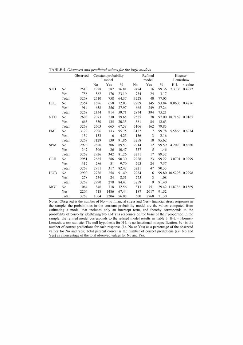
TABLE 4. Observed and predicted values for the logit models Observed Constant probability

model Refined model

Hosmer-Lemeshow

No Yes % No Yes % H-L p-value STD No 2510 1928 582 76.81 2494 16 99.36 7.3706 0.4972 Yes 758 582 176 23.19 734 24 3.17 Total 3268 2510 758 64.37 3228 40 77.05 HOL No 2354 1696 658 72.03 2209 145 93.84 8.0606 0.4276 Yes 914 658 256 27.97 665 249 27.24 Total 3268 2354 914 59.71 2874 394 75.21 NTO No 2603 2073 530 79.65 2525 78 97.00 18.7162 0.0165 Yes 665 530 135 20.35 581 84 12.63 Total 3268 2603 665 67.58 3106 162 79.83 FML No 3129 2996 133 95.75 3122 7 99.78 5.5866 0.6934 Yes 139 133 6 4.25 136 3 2.16 Total 3268 3129 139 91.86 3258 10 95.62 SPM No 2926 2620 306 89.53 2914 12 99.59 4.2070 0.8380 Yes 342 306 36 10.47 337 5 1.46 Total 3268 2926 342 81.26 3251 17 89.32 CLH No 2951 2665 286 90.30 2928 23 99.22 3.0701 0.9299 Yes 317 286 31 9.70 293 24 7.57 Total 3268 2951 317 82.48 3221 47 90.33 HOB No 2990 2736 254 91.49 2984 6 99.80 10.5293 0.2298 Yes 278 254 24 8.51 275 3 1.08 Total 3268 2990 278 84.43 3259 9 91.40 MGT No 1064 346 718 32.56 313 751 29.42 11.8736 0.1569 Yes 2204 718 1486 67.44 187 2017 91.52 Total 3268 1064 2204 56.08 500 2768 71.30 Notes: Observed is the number of No – no financial stress and Yes - financial stress responses in the sample; the probabilities in the constant probability model are the values computed from estimating a model that includes only an intercept term, and thereby corresponds to the probability of correctly identifying No and Yes responses on the basis of their proportion in the sample; the refined model corresponds to the refined model results in Table 3. H-L – Hosmer-Lemeshow test statistic. The null hypothesis for H-L is no functional misspecification. % - is the number of correct predictions for each response (i.e. No or Yes) as a percentage of the observed values for No and Yes; Total percent correct is the number of correct predictions (i.e. No and Yes) as a percentage of the total observed values for No and Yes.

ISSN 1324-5910 All correspondence to: Associate Professor Andrew C Worthington Editor, Discussion Papers in Economic, Finance and International Competitiveness School of Economics and Finance Queensland University of Technology GPO Box 2434, BRISBANE QLD 4001 Australia Telephone: 61 7 3864 2658 Facsimile: 61 7 3864 1500 Email: a.worthington@qut.edu.au

DISCUSSION PAPERS IN ECONOMICS, FINANCE

AND INTERNATIONAL COMPETITIVENESS

Debt as a Source of Financial Stress in Australian Households

Andrew Worthington

Discussion Paper No. 164 November 2003

Series edited by Associate Professor Andrew C Worthington

School of Economics and Finance

RECENT DISCUSSION PAPERS Drew, M E, Subramaniam, N & Clowes-Doolan, K, Students’ Experience o f the Honours’ Supervisory Relationship: A Preliminary Investigation, No 113, June 2002 Worthington, A, Kay-Spratley, A & Higgs, H, Transmission of Prices and Price Volatility in Australian Electricity Spot Markets: A multivariate GARCH Analysis, No 114, July 2002 Hernandez, J & Layton, A, The Regional Appropriateness of Monetary Policy: An Application of Taylor’s Rule to Australian States and Territories, No 115, August 2002 Taing, S H & Worthington, A, Co-movements Among European Equity Sectors: Selected Evidence from the Consumer Discretionary, Consumer Staples, Financial, Industrial and Materials Sectors, No 116, September 2002 Goffey, K & Worthington, A, Motor Vehicle Usage Patterns in Australia: A Comparative Analysis of Driver, Vehicle & Purpose Characteristics for household & Freight Travel, No 117, September 2002 Lahiri, R, On Optimal monetary Policy in a Liquidity Effect Model, No 118, October 2002 Valadkhani, A, Identifying Australia’s High Employment Generating Industries, No 119, October 2002 Valadkhani, A, Modelling Demand for Broad Money in Australia, No 120, December 2002 Worthington, A & Higgs, H, The Relationship Between Energy Spot and Futures Prices: Evidence from the Australian Electricity Market, No 121, November 2002 Li, S, A Valuation Model for Firms with Stochastic Earnings, No 122, November 2002 Higgs, H & Worthington, A, Tests of the Random Walk Hypothesis for Australian Electricity Spot Prices: An Application Employing Multiple Variance Ratio Tests, No 123, November 2002 Robinson, M, Best Practice in Performance Budgeting, No 124, November 2002 Lee, B, “Output and Productivity Comparisons of the Wholesale and Retail Trade Sector: US and Australia, 1991 to 1999”, No 125, November 2002 Drew, M E, & Stanford, J D, Risk Superannuation Management in Australia: Risk, Cost and Alpha, No. 126, January 2003

Drew, M E, & Stanford, J D, A Review of Australia's Compulsory Superannuation Scheme after a Decade, No. 127, January 2003 Drew, M E, & Naughton, T, & Veerarghavan, M, Asset Pricing in China: Evidence from the Shanghai Stock Exchange, No. 128, January 2003 Clements, A, & Drew, M E, Investor Expectations and Systematic Risk, No. 129, January 2003 Drew, M, Superannuation Funds: The Fees and Performance Debate, No. 130, January 2003 Valadkhani, A, History of Macroeconomic Modelling: Lessons from Past Experience, No. 131, January 2003 Valadkhani, A, Long and Short-Run Determinants of Money Demand in New Zealand: Evidence from CoIntegration Analysis, No. 132, January 2003 Anderson, J, Optimal f and Portfolio Return Optimisation in US Futures Markets, No. 133, January 2003 Anderson J, A Test of Weak-Form Market Efficiency in Australia Bank Bill Futures Calendar Spreads, No. 134, January 2003 Aruman, S, The Effectiveness of Foreign Exchange Intervention in Australia: A Factor Model Approach with GARCH Specifications, No 135, January 2003 Lahiri, R, A Further Exploration of Some Computational Issues in Equilibrium Business Cycle Theory, No 136, February 2003 Valadkhani, A, How Many Jobs Were Lost With the Collapse of Ansett? , No. 137, February 2003 Drew, M E, Naughton, T, & Veerarghavan, M, Is Idiosyncratic Volatility Priced? Evidence from the Shanghai Stock Exchange, No. 138, February 2003 Valadkhani, A, Does the Term Structure Predict Australia's Future Output Growth? No. 139, February 2003 Worthington, A, & Higgs, H, A Multivariate GARCH analysis of the Domestic Transmission of Energy Commodity Prices and Volatility: A comparison of the Peak and Off-peak Periods in the Australian Electricity Spot Market, No. 140, February 2003

Li, S, The Estimation of Implied Volatility from the Black-Scholes Model: Some New Formulas and Their Applications, No. 141, February 2003

Drew, M E, & Stanford, J D, Principal and Agent Problems in Superannuation Funds, No. 142, March 2003 Li, S, A Single-Period Model and Some Empirical Evidences for Optimal Asset Allocation with Value-at-Risk Constraints, No. 143, March 2003 Valadkhani, A, An Empirical Analysis of the Black Market Exchange Rate in Iran, No. 144, April 2003 Worthington, A, Business Expectations and Preferences regarding the Introduction of Daylight Saving in Queensland, No. 145, May 2003 Worthington, A, Losing Sleep at the Market: An Empirical Note on the Daylight Saving Anomaly in Australia, No. 146, May 2003 Robinson, M, Tightening the Results/Funding Link in Performance Budgeting Systems, No. 147, May 2003 Worthington, A & Higgs, H, Risk, Return and Portfolio Diversification in Major Painting Marketing: The Application of Conventional Financial Analysis to Unconventional Investments, No. 148, June 2003 Valadkhani A, Demand for M2 in Developing Countries: An Empirical Panel Investigation, No. 149, July 2003 Worthington A, & Higgs H, Modelling the Intraday Return Volatility Process in the Australia Equity Market: An Examination of the Role of Information Arrival in S & PASX Stocks, No 150, July 2003 Lahiri R, Tax Distortions in a Neoclassical Monetary Economy in the Presence of Administration Costs, No 151 September 2003 Layton A, & Smith D, Duration Dependence in the US Business Cycle, No 152, August 2003 Valadkhani A & Layton A, Quantifying the Effect of GST on Inflation in Australia’s Capital Cities: An Intervention Analysis, No 153, September 2003 Worthington A, & Valadkhani A, Measuring the Impact of Natural Disasters on Capital Markets: An Empirical Application Using Intervention Analysis, No 154, September 2003

Robinson M, The Output Concept and Public Sector Services, No 155, September 2003 Worthington A, Brown K, Crawford M, & Pickernell D, Socio-Economic and Demographic Determinants of Household Gambling in Australia, No 156, September 2003 Worthington A, & Higgs H, Tests of Random Walks and Market Efficiency in Latin American Stock Markets: An Empirical Note, No 157, September 2003 (Replacing Previous No 158) Worthington A, & Higgs H, Systematic Features of High-Frequency Volatility in Australian Electricity Markets: Intraday Patterns, Information Arrival and Calendar Effects, No 158, November 2003 Worthington A, & Higgs H, Weak-form Market Efficiency in European Emerging and Developed Stock Markets, No 159, September 2003 West T, & Worthington A, Macroeconomic Risk Factors in Australian Commercial Real Estate, Listed Property Trust and Property Sector Stock Returns: A Comparative Analysis using GARCH-M, No 160, October 2003 Lee, B, Interstate Comparison of Output and Productivity in the Australian Agricultural Sector – 1991 – 1999, No 161, October 2003 McCarthy S, Hedging Versus not Hedging: Strategies for Managing Foreign Exchange Transaction Exposure, No 162, November 2003 Worthington, A, Emergency Finance in Australian Households: An Empirical Analysis of Capacity and Sources, No 163, November 2003