BAYESIAN DECISIONS UNDER TOTAL AND PARTIAL IGNORANCE

by

Dean Jamison

and

SUBJECTIVE PROBABILITIES UNDER TOTAL UNCERTAINTY

by

Dean Jamison and Jozef Kozielecki

TECHNICAL REPORT NO. 121

September 4, 1967

PSYCHOLOGY SERIES

Reproduction in Whole or in Part is Permitted for

any Purpose of the United States Government

INSTITUTE FOR MATHEMATICAL STUDIES IN THE SOCIAL SCIENCES

STANFORD UNIVERSITY

STANFORD, CALIFORNIA

TABLE OF CONTENTS

Page

Bayesian Decisions under Total and Partial Ignorance • • • • • •• 1

Subjective Probabilities under Total Uncertainty • • • • • • • • • 23

ii

. BAYESIAN DECISIONS UNDER TOTAL AND PARTIAL IGNORANCEl

by

Dean Jamison

Introduction

1. A triple P = < D, n, U > may be considered a finite deci.ion

problem when: (i) D is a finite set of alternative courses of action

available to a decision-maker, (ii) n is a finite set of mutually exclu-

sive and exhaustive possible states of nature, and (iii) U is a function

on D X n such that u( d., w.)1 J

is the utility to the decision-maker if

he chooses di and the true state of nature turns out to be w.. AJ

decision procedure (solution) for the problem P consists either of an

ordering of the di according to their desirability or of the specifi-

cation of a subset of D that contains all di that are in some sense

optimal and only those di

that are optimal.

The set of all possible

n, that is, the set of all vectors whose

--;

If there are m states of nature, a vector ~ = (~1'~2'

is a possible probability distribution over n (with prob(w.)m J

iff ') ~. = 1 and ~. > 0 for 1 _< j_< m.J'-;;]. J J -

probability distributions over

... ,~ )m

components satisfy the above equation and set of inequalities, will be

denoted by Atkinson, Church, and Harris (1964) assume our knowl---;

edge of ~ to be completely specified by asserting that

~"......., ~---../

where - c::J. If z. = z" they say we are in complete ignorance of""""0- 0

--;

~. In the manner of Chernoff (1954) and Milnor (1954), Atkinson, et al,

give axioms stating desirable properties for decision procedures under

complete ignorance. A class of decision procedures that isolate an

optimal subset of D is shown to exist and satisfy the axioms. Efron (1965)

2

extends the range of applicability of the decision procedures suggested

by Atkinson, et aI, and dubs them "iterated minimax regret rules". These

rules are non-Bayesian in the sense that the criterion for optimality is

not maximization of expected utility. Other non-Bayesian decision pro-

cedures for complete ignorance (that fail to satisfy some axioms that

most people would consider reasonable) include the following: minimax

regret, minimax risk (or maximin utility), and Hurwicz's a procedure

for extending the minimax risk approach to non-pessimists.

The Bayesian alternative to the above procedures attempts to order

the d, according to their expected utility; the optimal act is, then,1

simply the one with the highest expected utility. Computation of the

expected utility of di

, Cur di ), is straightforward if the decision-

is a set with but one element

Only in the rare instances when considerable

maker knows that '~--- "0

m *C.U(d,) = LU(d" w,)g,.

1 'I 1 J JJ=relative frequency data exist will the decision-maker be able to assert

rJthat.~o has only one element. In the more general case the decision-

maker will be in "partial" or "total" ignorance concerning the probability

vector r. It is the purpose of this paper to characterize total and

partial ignorance from a Bayesian point of view and to show that decision

procedures based on maximization of expected utility extend readily to

these cases.

Decisions under Total Ignorance

2. Rather than saying that our knowledge of the probability vector

t is specified by asserting that for some ~o' I suggest that

it is natural to say that our knowledge of r is specified by a density,

f(gl' g2' ... , gm)' defined on;::::. If the probability distribution over

3

n is known to be -g*, then f is a 1) function "t r* and computation

of tU(di) proceeds as in the Introduction. At the other extreme from

precisely knowing the probability distribution over n is the case of.".

total ignorance. In this section a meaning for "total ignorance" of ~

will be suggested and decision-making under total ignorance will be dis-

cussed. In the following section decisions under partial ignorance----7

anywhere between knowledge of S and total ignorance--will be discussed ..".

3. If H(S) is the Shannon (1949) measure of uncertainty concerning

-d m H( t')which W in n occurs, then H(S) ~ L S. log2 (l/Si)' where " isio=l ~

measured in bits. When this uncertainty is a maximum, we may be considered

in total ignorance of wand, as one would expect, this occurs when we

have no reason to expect anyone W more than another, i.e., when

S. 0= l/m for 1 < i < m. By analogy, we can be considered in total~

ignorance of r when H(f) ~JJ'i;;Jf(r) lOg2(1/f(t)) d;<; is a maximum.

This occurs when f is a constant, that is, when we have no reason to

F (expect one value of " to be more probable than any other see Shannon

(1949), Ch. 3). If there is total ignorance concerning t, then it is

reasonable to expect that there be total ignorance concerning W --and

this is indeed true (if we substitute the expectation of Si' S(Si)'

for Si)2. Let me now prove this last assertion, which is the major

result of this section.

4. Proving that under total ignorance [(S.) ~ l/m involves, first,~

determination of the appropriate constant value of f, then determination

of the probability density functions for the SiS and, finally,' integration

to find €,( S. ) .~

Let the constant value of f(Sl' S2' ... , Sm) be equal to K; since

f is a density, the integral of K over ~ must be unity:

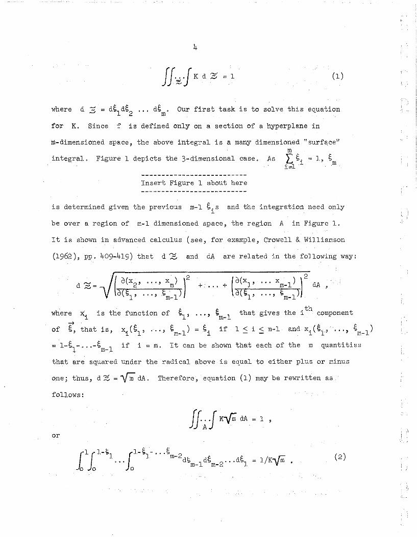
4

(1)

where d ~ = dSl dS2

'" dSm

, Our first task is to solve this eQuation

for K. Since f is defined only on a section of a hyperplane in

m-dimensioned space, the above integral is a many dimensioned "surface"m

integral. Figure 1 depicts the 3-dimensional case, As I: s. = 1, S• , l ml:::::J..

Insert Figure 1 about here

is determined given the previous m-l S.sl

and the integration need only

be over a region of m-l dimensioned space, the region A in Figure 1.

It is shown in advanced calculus (see, for example, Crowell &Williamson

(1962), pp. 409-419) that d:::' and dA are related in the following way:

... ,

d Z:=

where Xi is the function of Sl'->

of S, that is, xi(Sl' ... , Sm_l)

2+ .. , + (O(Xl , x m_l ) 1 dA,

d(Sl' , Sm_l)'

" th t· th' th t~ a glves e l componenm-l

= l-SJ,.-" '-Sm_I if i = m. It can be shown that each of the m quanti ties

that are squared under the radical above is eQual to either plus or minus

one; thus, d?'!- =~ dA. Therefore, equation (1) may be rewritten as

follows:

or

l/K....r; . (2)

(1,0,0)

Figure L :=., the set o:f possible probability distributions over 110

5

The multiple integral in (2) coul~ conceivably be evaluated by

iterated integration; it is much simpler, however, to utilize a technique

Dirichlet showed the following

is defined in thedevised by Dirichlet. Recall that the gamma function

() J00 n-l -xfollowing way: r n = x e dx for n > O. If

ointeger, r (n) = (n-l)~ and O~ = 1.

n is a positive

(see Jeffreys and Jeffreys (1956), pp. 468-470): If A is the closed

region in the first ortant bounded by the coordinate hyperplanes and byp, P2 Pn

the surface (xl/cl).L + (x2 /c2

) + ... + (xn/cn ) = 1, then

(Xl (X2

r( l + - +-+P P •..1 2

For our purposes, c. = p. = (X, = 1, :for 1 < i < m and the m-l £.. s1 1 ~ 1

replace the n xs. The result is that the integral in (2) becomes

l/r(m) = l/(m-l)~. Therefore K = (m-l)~....r;;/m.

Having determined the constant value, K, of f we must next determine

the densities fi(£i) for the individual probabilities, By symmetry,

the densities must be the same for each The densities are the

derivatives of the distribution functions which will be denoted

Fl(c) gives the probability that £1 is less than c; denote by

F. (£. ).1. 1.

*Fl(C)

the probability that £1 ~ c, that is, Fl(C) is

simply the integral of

all points such that

f over Z, where~c

£1 ~ c. See Fig. 2.

is the subset of ~ including

is given by:

Insert Figure 2 about here

6

(4 )

Since K = (m-l)~ ,Jrn/m, (4) becomes (after inserting the limits of

A translation of the Sl axis will enable us to use Dirichlet integration

to evaluate (5 ) ; let S' = Sl- c. Then S~ + S2 + ... + Sm-l = l-c, or1 m-l

S~/(l-C) + S2/(1-C) + ... + Sm_l/(l-c) - 1 ( since L S. = 1 is thei=l

1

boundary of the region A). Referring back to equation (3 ) it can be seen

that the c.s in that equation are all equal to l-c and that, therefore,1

the integral on the r.h.s. of (5) is

(l_C)m-l/r{m) = (l_c)m-l. Therefore

(l_C)m-l/r{m). Thus F~(C) = (m-l)'.

F (c) = 1 - (l_C)m-l. Since this1

holds if c is set equal to any value of Sl between 0 and 1, Sl

can replace c in the equation; differentiation gives the probability

density function of Sl and hence of all the SiS:

Recourse to a table of integrals will

f.(S.) = (m-l)(l-S. )m-21 1 1

From (6) the expectation of S. is easily computed-­1

(' (s.) =1\. (m-l)(l-S. )m-2G 1. ,1. 1.o

quickly convince the reader that ~(Si) = 11m. Figure 3 shows

(6)

f.(S.)1 1

for several values of m.

Insert Figure 3 about here

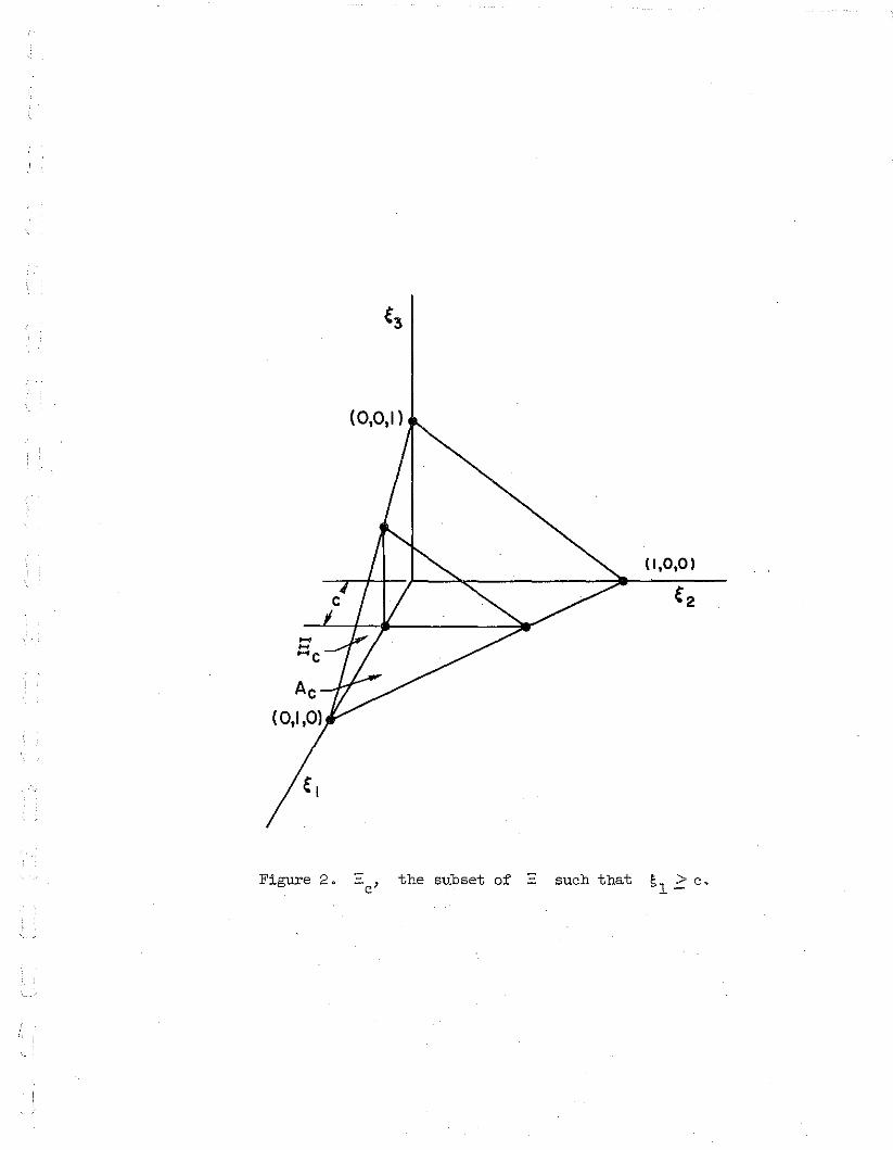
(1,0,0 )

Figure 20 the subset of _ such that s1 ::: Co

6

5

4

t...

Figuxe 3~ Marginal densities under total uncertainty.•

of di is given by:

5 . Let u(d., ~)1

7

Then the expected utility

.".u(d., £)

1

£u(d.) =If.· ·fK u(d., r)d~.1 ,Z 1·

m mThis is equal to L((£.) u(d., w.) = (11m) L u(d.,

'1 J 1 J '1 1J= J=is a linear function of the random variables

(1965), p. 126ff.)

since

(See Lindley

Thus, taking the view of total ignorance adopted herein, we arrive

at the decision rule advocated by Bernoulli and Laplace and axiomatized

in Chernoff (1954), This decision rule is claimed to have two defects.

Firstly,what to call a distinct state of nature is often an arbitrary

choice, and, secondly, the rule cannot deal with an infinite number of

states of nature. I think these defects are unimportant.

Assume that all utilities are normalized to the interval between

zero and one and that e represents a utility so small as to be of no

practical importance to the decision-maker. Then all utilities can be

rounded off to the nearest of a total number of lie distinct utility

points between zero and one. If there are a finite number, n, of decisions

npossible, there can be no more than (lie) different utility columns.

For example if lie = 3 and n = 2, the matrix below contains all the

different utility columns.

8

Adding another column would only duplicate a previous one. By grouping

together all "states of nature" that yield identical utility columns,

the decision-maker has a minimum of at most (l/E)n (and usually far fewer)

states of nature to consider. This is a practical solution to the problem

of an infinite number of states of nature. The decision-maker may choose

to consider more than the minimum number of states of nature if he wishes

to regard as different two distinct sets of physical circumstances that

yield identical utility columns. That seems to me to be a matter of

individual taste.

The last sentence in the preceding paragraph suggests that the

same decision problem may justly be formulated in many ways and that

the choice among the alternatives is up to the decision-maker. Clearly

if Bayesian decision procedures for total ignorance were used in each

formulation of the problem, then the d. chosen could depend on the~

formulation. However, changing the formulation of the problem gives us

information about the new set of outcomes. For example, if we collapse

two exclusive states of nature into one, the probability of the new state

must be considered the sum of the probabilities of the old ones, and we

can no longer be considered in total ignorance of the outcome. In fact,

very rarely will we be in a decision situation of total ignorance;

usually there will be some partial information. To this class of problems

we now turn.

Decisions under Partial Ignoranc~

6. Partial ignorance exists in a given formulation of a decision

if we neither know the probability distribution over n nor are in total

ignorance of it. If we are given f(~l' ~2' .,. ~m)' the density over

computation of Eu( d. )1

9

under partial ignorance is in principle

straightforward and proceeds along lines similar to those developed in

the previous section, Equation (7) is modified in the obvious way to:

(8)

If f is any f the large variety of appropriate forms indicated just

prior to equation (3), the integral in (8) may be easily evaluated using

Dirichlet integration; otherwise, more cumbersome techniques must be used.

In practice it seems clear that unless the decision-maker has

remarkable intuition, the density f will be impossible to specify from

the partial information at hand. Fortunately there is an alternative to

determining f.

7. Jeffrey (1965, pp. 183-190), in discussing degree of confidence

of a probability estimate, describes the following method for obtaining

the distribution function, Fi

(5i), for a probability. Have the decision-

maker indicate for numerous values of 5. what his subjective estimate1

is that the "true" value of 5i

is less than the value named. To apply

this to a decision problem the distribution function--pnd hence

for each of the Sis must be obtained. Next, the expectations of the

Sis must be computed and, fr6m them, the expected utilities of the dis

can be determined. In this way partial information is processed to lead

to a Bayesian decision under partial ignorance.

It should be clear that the decision-maker is not free to choose

the fis subject only to the condition that for each f i , j lf i (51 )d5i 1.

o 'Consider the example of the misguided decision-maker who believed himself

to be in total ignorance of the probability distribution over 3 states of

10

nature. Since he was in total ignorance, he reasoned, he must have a

uniform p.d.f. for each £..1

That is,

for 0 < £. < 1. If he believes these to be the p.d.f.s, he should be1 -

willing to simultaneously take even odds on bets that £1 > 1/2,

£2 > 1/2, and 63

> 1/2. I would gladly take these three bets, for under

no conditions could I fail to have a net gain. This example illustrates

the obvious -- certain conditions must be placed on the f. s1

in order that

they be coherent. A necessary condition for coherence is indicated below;

I have not yet derived sufficient conditions.

Consider a decision, dk

, that will result in a utility of 1 for

each w.. Clearly, then, c: u( dk ) =1. However, t u( dk ) also equalsJ

l(61 )U(dk ,wl ) + + C:J £ )u( d ,w ). Since for 1 < i < m,m k m

u(dk,wi ) = 1, a necessary condition for coherence of the fis is thatm~((6.) = 1, a reasonable thing to expect. That this condition is noti=l 1

sufficient is easily illustrated with two states of nature. Suppose

that f l (61 ) is given. Since £2 = 1 - £1' f 2 is uniquely determined

given fl' However it is obvious that infinitely many f 2s will

satisfy the condition that (.(62

) -- 1 - [( 61

), and if a person were to

have two distinct f 2s it would be easy to make a book against him; his

beliefs would be incoherent.

If m is not very large, it would be possible to obtain condi-

tional densities of the form f2(62161)' f3

(63 IS1 '£2)' etc., in a

manner analogous to that discussed by Jeffrey. If the conditional

densities were obtained, then

expression:

"""f(6) would be given by the following

11

A sufficient condition that the f.s be coherent is that the integral ofl

f over ~ be unity; if it differs from unity, one way to bring about

coherence would be to multiply f by the appropriate constant and then

find the new f.s. If m is larger than 4 or 5, this method of insuringl

coherence will be hopelessly unwieldy. Something better is needed.

8. At this point I would like to discuss alternatives and

objections to the theory of decisions under partial information that

is developed here. The notion of probability distributions over proba-

bility distributions has been around for a long time; Knight, Lindall,

and Tintner were among the first to explicitly use the notion in

economics (see Tintner (1941».3 This work has not, however, been

formulated in terms of decision theory. Hodges and Lehmann (1952)

have proposed a decision rule for partial ignorance that combines the

Bayesian and minimax approaches. Their rule chooses the d. thatl

maximizes [u( d. )l

for some best estimate (or expectation) of

subject to the condition that the minimum utility possible for d.l

is

greater than a preselected value. This preselected value is somewhat less

than the maximum utility; the amount less increases with our confidence

that t is the correct distribution over Q. Ellsberg (1961), in the

lead article of a spirited series in the Quarterly Journal of Economics,

provides an elaborate justification of the Hodges and Lehmann pro-

cedure, and I will criticise his point of view presently.

Hurwicz (1951) and Good (1950) (discussed in Luce and Raiffa (1956),

p. 305) have suggested characterizing partial ignorance in the same

fashion that was later used by Atkinson, et al (1964). That is, Our

knowledge of

12

r is of the form r~owhere ;::;; is a subset of ::s

Hurwicz then prDposes that we proceed as if in total ignorance of where

r is in In the spirit of the second section of this paper, the

decision rule could be Bayesian with for and

f(D = a elsewhere, Hurwicz suggests instead utilization of nOn-

Bayesian decision procedures; difficulties with non-Bayesian procedures

were alluded to in the Introduction,

The reader interested in a more thorough discussion and bibliog-

raphy concerning decisions under total and partial ignorance is referred

to Arrow (1951), Luce and Raiffa (1956), and Luce and Suppes (1965), I

will now try to conter some objections that have been raised against

characterizing partial ignorance as probability distributions over

probabilities,

On page 659 Ellsberg (1961) takes the view that since representing

partial ignorance (ambiguity) as a probability distribution over a

distribution leads to an expected distribution, ambiguity must be

someting different from a probability distribution, I fail to under-

stand this argument; ambiguity is high, it seems to me, if f is

relatively flat Over ~ otherwise not 0 The "reliability, credibility,

or accuracy" of one's information simply determines how sharply peaked

f is, Even granted that probability is somehow qualitatively different

from ambiguity or uncertainty, the solution devised by Hodges and

Lehmann (1952) and advocated by Ellsberg relies on the decision-maker's

completely arbitrary judgment of the amount of ambiguity present in the

decision situation, Ellsberg would have us hedge against our uncertainty

in r by rejecting a decision that maximized utility against the

13

expected distribution but that has a possible outcome with a utility

below an arbitrary minimum. By the same reasoning one could "rationally"

choose dl

over d2

in the non-ambiguous problem below if, because of

our uncertainty in the outcome, we said (arbitrarily) that we would

reject any decision with a minimum gain of less than 3.

w w1 2

dl 5 5sl = s2 = .5

d2 1 25

I would reject Ellsberg's approach for the simple reason that its

pessimistic bias leads to decisions that fail to fully utilize one's

partial information.

Savage (1954, pp. 56-60) raises two objections to second-order

probabilities. The first, similar to Ellsberg's, is that even with

second-order probabilities expectations for the primary probabilities

remain. Thus we may as well have simply arrived at our best subjective

estimate of the primary probability, since it is all that is needed for

decision-making. This is correct as far as it goes, but, without

second-order probabilities, it is impossible to specify how the primary

probability should change in the light of evidence. This will be

discussed in more detail in the final section.

Savage's second objection is that" ... once second order probabil-

ities are introduced, the introduction of an endless hierarchy seems

inescapable. Such a hierarchy seems very difficult to interpret, and it

seems at best to make the theory less realistic, not more." Luce and

Raiffa (1956) express much the same objection on page 305. An endless

14

hierarchy does not seem inescapable to me; we simply push the hierarchy

back as far as is required to be "realistic". In making a physical

measurement we could attempt to specify the value of the measurement,

the probable error in the measurement, the probable error in the probable

error, and on out the endless hierarchy. But it is not done that way;

probable errors seem to be about the right order of realism. Similarly,

I suspect that second-order probabilities will suffice for most circum-

4stances.

15

The Role of Evidence in Changing Probabilities

9. The preceding: discussion has been limited to situations in

which the decision-maker has no option to experiment or buy information.

When the possibility of experimentation is introduced, the number of

alternatives open to the decision-maker is greatly increased, as is the

complexity of his decision problem, for the decision-maker must now

decide which experiments to perform and in what order; when to stop

experimenting; and which course of action to take when experimentation

is complete. (See discussion in Chap. 3 of Blackwell and Girshick

(1954).) A crucial question here is to specify how evidence is to be

used to change our probability estimates.

If we are quite certain that r is very nearly the true probability

distribution over ~,additional evidence will little change Our beliefs.

If, on the other hand, we are not at all confident about -r -- if f is

fairly flat --, new evidence can change Our beliefs considerably. (New

evidence may leave the expectations for the SiS unaltered even though

it changes beliefs by making f more sharp. In general, of course,

new evidence will both change the sharpness of f and change the

expectations of the S. s. )1

Without second-order probabilities there

appears to be no answer to the question of exactly how new evidence can

alter probabilities. Suppes (1956) considers an important defect of both

his and Savage's (1954) axiomatizations of subjective probability and

utility to be their failQre to specify how prior information is to be

used. Let us consider an example used by both Suppes and Savage.

10. A man must decide whether to buy some grapes which he knows

to be either green (Wl ), ripe (W2

), or rotten (W3

). Suppes poses the

16

following que~tion: If the man has purchased grapes at this store 15

times previously, and has never received rotten grapes, and has no

information aside from these purchases, what probability should he assign

to the outcome of receiving rotten grapes the 16th time?

Prior to his first purchase, the man was in total ignorance of the

probability distribution over Thus from equation (6) we see that

the density for S3' the prior probability of receiving rotten grapes,

should be f3

(S3) = 2 - 2 S3' Let X be the event of receiving green

or ripe grapes on the first 15 purchases; the probability that X occurs,

isgiven s3 '

the density for

p(xI S3 ) = (1 - S3)15, 'What we desire is f3(S3Ix),

s3 given X, and this is obtained by Bayes' theorem in

the following way:

(10)

After inserting the expressions for f3

(S3) and p(xl s3 ), equation

(10) becomes:

Performing the integration and simplifying gives f3(S3Ix) = 17(1 S3)16;

from this the expectation of s3 given X can be computed --

[(S 31x) = 17.fa\ 3(1 - S3)16 = 1/18, (Notice i:;hat this result differs

from the 1/17 that Laplace's law of succession would give, The

difference is due to the fact that the Laplacian law is derived from

consideration of only two states of nature -- rotten and not rotten5,)

17

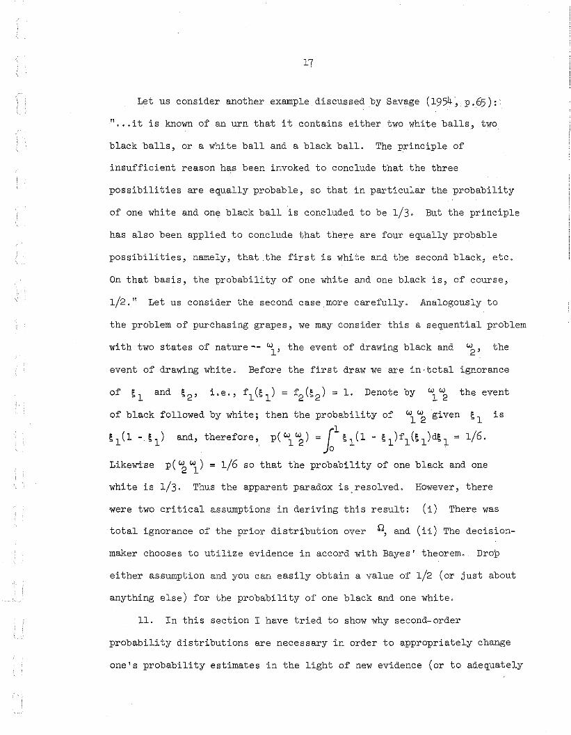
Let us consider another example discussed by Savage (1954, P ;65):,

" ... it is known of an urn that it contains either two white balls, two

black balls, or a white ball and a black ball. The principle of

insufficient reason has been invoked to conclude that the three

possibilities are equally probable, so that in particular the probability

of one white and one black ball is concluded to be 1/3. But the principle

has also been applied to conclude that there are four equally probable

possibilities, namely, that the first is white and the second black, etc.

On that basis, the probability of one white and one black is, of course,

1/2." Let us consider the second case more carefully. Analogously to

the problem of purchasing grapes, we may consider this a sequential problem

with two states of nature"" wl ' the event of drawing black and W2' the

event of drawing white. Before the first draw we are in,total ignorance

of ~l and ~2' Le., fl(~l) ~ f2(~2) = 1. Denote by w12 the event

of black followed by white; then the probability of wl w2

given ~l is

~l(l" ~l) and, therefore, p(W12 ) =fcl~l(l" ~l)fl(~l)d~l = 1/6.

Likewise p( 2 'J) = 1/6 so that the probability of one black and one

white is 1/3. Thus the apparent paradox is,resolved. However, there

were two critical assumptions in deriving this result: (i) There was

total ignorance of the prior distribution over ~,and (ii) The decision-

maker chooses to utilize evidence in accord with Bayes' theorem. Drop

either assumption and you can easily obtain a value of 1/2 (or just about

anything else) for the probability of one black and one white.

11. In this section I have tried to show why second-order

probability distributions are necessary in order to appropriately change

one's probability estimates in the light of new evidence (or to adequately

18

utilize one's prior information). My discussion is primarily suggestive;

it fails to deal with any of the difficult features of sequential decision­

making alluded to at the beginning of this section. Yet the relevance of

second-order probabilities to these problems should be clear. A more

complete theory of Bayesian decisions under partial ignorance will be

required to deal with decision situations where experimentation is allowed.

Suppes' (1965) suggestion for introducing a theory of confirmation or

inductive logic at the foundations of decision theory should be considered

in the light of second-order pFobabilities and Bayes' theorem. The

relation between evidence and information should be clarified and a theory

of the value of evidence as based on its information content should be

developed.

19

References

Arrow, K, Alternative approaches to the theory of choice in risk taking

situations, Econometrica, 1951, 19, 404-437.

Atkinson, F" Church, J" & Harris, B, Decision procedures for finite

decision problems under complete ignorance, Annals of Mathematical

Statistics, 1964, 35, 1644-1655,

Blackwell, D" & Girshick, M, A, Theory of Games and Statistical

Decisions. New York: John Wiley, 1954.

Chernoff, H. Rational selection of decision functions. Econometrica,

1954, 22, 422-443.

Crowell, R. H., & Williamson, R. E. Calculus of Vector Functions.

Englewood Cliffs, New Jersey: Prentice Hall, 1962.

Efron, B. Note on decision procedures for finite decision problems

under complete ignorance. Annals of Mathematical Statistics, 1965,

Ellsberg, D, Risk, ambiguity, and the savage axioms. Quarterly

Journal of Economics, 1961, 75, 643-669,- -Good, I. J. Probability and the Wei8hing of Evidence. London: Chas.

Griffin and Co" 1950.

Good, I. J. The Estimation of Probabilities: An Essay £g Modern

Bayesian Methods, Cambridge: MIT Press, 19650

Hodges, J., & Lehmann, E, The use of previous experience in reaching

statistical decisions. Annals of Mathematical Statistics, 1952,

23, 396-407.

Howard, R. A. Prediction of replacement demand, In Go Kreweras and

G. Morlat (Eds.), Proceedin8s of the Third International Conference

on Operational Research. London: English Universities Press, Ltd.,

1963, pp. 905-918,

20

Hurwicz, L. Some specification problems and applications to econometric

models (abstract). Econometrica, 1951, 19, 343-344.

Jeffrey, R. The Logic of Decision. New York: McGraw-Hill, 1965.

Jeffreys, H., & Jeffreys, B. S. Mathematical Physics. Cambridge:

The University Press, 1956.

Lindley, D. V. Probability and Statistics from ~ Bayesian Viewpoint,

Vol. I. Cambridge: The University Press, 1965.

Luce, R. & Raiffa, H. Games and Decisions: Introduction and Critical--------Survey. New York: John Wiley, 1956.

Luce, R. & Suppes, P. Preference, utility, and subjective probability.

In R. Bush, E. Galanter, and R. Bush (Eds.), Handbook of

Mathematical Psychology, Vol. III. New York: John Wiley, 1965.

Pp. 249-410.

Milnor, J. Games against nature. In C. Coombs, R. Davis, and R. Thrall

(Eds.), Decision Processes. New York: John Wiley, 1954.

Reprinted in M. Shubik (Ed.),~ Theory~ Related Approaches

to Social Behavior. New ·York: John Wiley, 1964. Pp. 120-131.

Savage, L. J. The Foundations £f Statistics. New York: John Wiley, 1954.

Shannon, C. E., & Weaver, W. 1lJ&. Mathematical Theorx of Communication.

Urbana: University of Illinois Press, 1949.

Suppes, P. The role of subjective probability and utility in decision-

making. In R. Bush, E. Galanter, and R. Luce (Eds.), Readings in

Mathematical Psychology, Vol. II. New York: John Wiley, 1965.

Pp.503-515. Reprinted from the Proceedings of the Third Berkeley

Symposium ££ Mathematical Statistics and Probability, 1954-1955.

Tintner, G. The theory of choice under subjective risk and uncertainty.

Econometrica, 1941, 2, 298-304.

21

Footnotes

1The author is deeply indebted to Professors Patrick Suppes and

Howard Smokler for helpful advice and comments concerning this paper.

The author has had a number of helpful conversations with Professor

John Br~akwell, Professor Donald Dunn, Professor Ronald Howard, Mr. Joe

Good, and Mr. Michael Raugh. The advice of these persons does not, of

course, necessarily imply their consent to the conclusions of the paper.

2Usually we can characterize the uncertainty in a decision

--.situation as the sum of H( t (~ )) and H( f). If, however, f itself

is not precisely known, the uncertainty associated with alternative

possible fs must be added in, and so on.

1.R. A. Howard (1963) utilizes what are essentially probability

distributions over probability distributions by considering a probability

density function for the parameters of another probability density

function.

4Professor Suppes points out to me that, though there is a rich

body of results in meta-mathematics, mathematicians apparently feel no

need to derive formal results concerning meta-mathematics in a meta_

meta-mathematics.

2-Laplace's law of succession is derived from Bayes' theorem and the

If the uniform prior is changedassumption of a uniform prior for

to any of the possibilities given

~ ..l

in equation (6), the fallowing

generalization of the law of succession can be derived: p (w)­r+l i -

(n + l)/(r + m), where Pr+l(Wi ) is the (expectation of) the probability

22

that on the r + 1st trial wi will occur, n is the number of times

it has occurred in the previous r trials, and m is the number of

states of nature. Since I completed this paper, Mr. R. Toumela has

pointed out to me that Good (1965) has discussed notions that are->

formally analogous to f(s). Good mentions that this generalized

version of the law of succession was known to Lidstone in 1925.

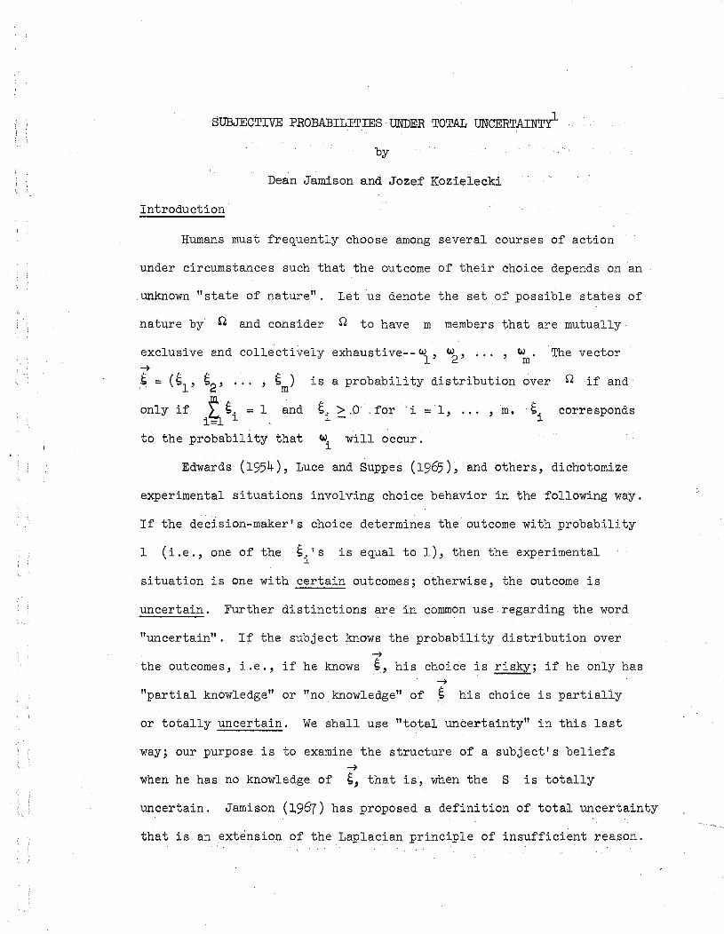
SUBJECTIVE PROBABILITIES UNDER TOTAL UNCERTAINTY-

by

Dean Jamison and JoZef Kozielecki

Introduction

Humans must frequently choose among several courses of action

under circumstances such that the outcome of their choice depends on an

unknown "state of nature". Let us denote the set of possible states of

nature by Q and consider Q to have m members that are mutually

exclusive and collectively exhaustive-- wl

, w2

' ... , W •m

The vector-->g = (51' 52' ...

only if ~ 5. = 1i~ l

5) is a probability distribution overm

and 5i >.0 . for i = 1, .. , ,m. 5i

Q if and

corresponds

to the probability that Wi will occur.

Edwards (1954), Luce and Suppes (1965), and others, dichotomize

experimental situations involving choice behavior in the following way.

If the decision-maker's choice determines the outcome with probability

1 (i.e., one of the 5.'s is equal to 1), then the experimentall

situation is One with certain outcomes; otherwise, the outcome is

uncertain. Further distinctions are in common use regarding the word

"uncertain". If the subject knows the probability distribution over-->

the outcomes, i.e., if he knows S, his choice is risky; if he only has-->

"partial knowledge" or "no knowledge" of 5 his choice is partially

or totally uncertain. We shall use "total uncertainty" in this last

way; our purpose is to examine the structure of a subject's beliefs-->

when he has no knowledge of 5, that is, when the S is totally

uncertain. Jamison (1967) has proposed a definition of total uncertainty

that is an extension of the Laplacian principle of insufficient reason.

24

This definition and some of its implications will be described briefly

here as theoretical background for our experimental results.

Consider the set of all possible probability distributions over

"'""Q, that is, the set of all vectors S. ~

Let us denote this set by :::-

= (0, 1, 0, .... , 0), or

If

and describe the decision-maker's knowledge of

"'""f(Sl' S2' '" , 5m) = f(g) defined on ::

"'"" "'""(0 function) at S = (1, 0, ... , 0) or S

by a density

is an impulse

o •• ,"'""~=(O,O, , 1), then decision-making is under certainty. If

"'""f(g) is an impulse elsewhere in ;:;:; the decision-making is risky. If

"'""f(S) is a constant, the decision-maker is, by definition, totally

"'""uncertain of S. The intuitive motivation for this definition is that

"'""if f(~) is a constant, no probability distributions over Q are more

likely than any others. Partial uncertainty occurs when f(S) is

2neither an impulse nor a constant.

If K is the constant value of f(~) under total uncertainty,

then:

Evaluating this definite integral enables us to find K, which turns

out to be (m - l)~~ 1m. The probability that 51 is greater than

some specific value, say C, is given by:

j lfl-Sljl-Sl-g2-,,,-Sm_2. (prob(Sl> C) = Co'" 0 'I'illKdSmc2dSm_3· .. dSl

= (1 _ c)m-l.

One minus prob(Gl

> C) is simply the probability that Sl ~ C or

toe cumulative marginal for Sl'

By symmetry Fl(C) = F2 (C) = '"

which we shall denote by Fl(C).

= F.(C) = ...F (C); thus we have:l m

25

F.(C) ~ l _ (1 _ C)m-l.~

Fig. l shows Fi(C) for several values of m.

Insert Fig. 1 about here

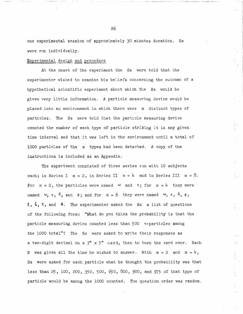
The derivative of the marginal cumulative is the marginal

densi ty, which we shall denote

dF. (C)f.(C) ~ ~l_

l dc

f. (C) :l

~ (m - 1)(1 _ c)m-2. (4 )

Fig. 2 shows f.(C)l

for several values of m.

Insert Fig. 2 about here

The purpose of our experiment was to determine if the normative

model just described for belief under total uncertainty approximates

the actual structure of Ss beliefs. To achieve this purpose we

placed Ss in a situation of total uncertainty and then empirically

determined the cumulative F.(C) for a number of values of m.l

Method

Subjects

The Ss were 30 students from Stanford University fulfilling

course requirements for introductory psychology. Each participated in

26

one experimental session of approximately 30 minutes duration, Ss

were run individually,

Experimental design~ procedure

At the onset of the experiment the Ss were told that the

experimenter wished to examine his beliefs concerning the outcome of a

hypothetical scientific experiment about which the Ss would be

given very little information, A particle measuring device would be

placed into an environment in which there were m distinct types of

particles, The Ss were told that the particle measuring device

counted the number of each type of particle striking it in any given

time interval and that it was left in the environment until a total of

1000 particles of the m types had been detected, A copy of the

instructions is included as an Appendix,

The experiment consisted of three series run with 10 subjects

each; in Series I m ~ 2, in Series II m ~ 4 and in Series III m ~ 8,

For m ~ 2, the particles were named w and E' for m ~4 they were,

named w, E, 6 and W; and for m ~ 8 they were named w, E, 6, W,,s, ~, X, and e, The experimenter asked the Ss a list of ~uestions

of the following form: "what do you think the probability is that the

particle measuring device counted less than 500 E-particles among

the 1000 total"? The Ss were asked to write their responses as

a two-digit decimal on a 3" x 5" 'card, then to turn the card over, Each

S was given all the time he 'wished to answer, With m ~ 2 and m ~ 4,

Ss were asked for each particle what he thought the probability was that

less than 25, 100, 200, 350, 500, 650, 800, 900, and 975 of that type of

particle would be among the 1000 counted, The ~uestion order was random,

Figure 10 Marginal c)llllulatives under total uncertainty.

7

6

5m=6

4Fj (Cl

3

2 m=2

Figure 20 Marginal densities under total uncertaintyo

27

For m = 8 the 350, 650, and 975 ~uestions were deleted. After the

experiment Ss were asked ~uestions concerning their method of

answering.

Results

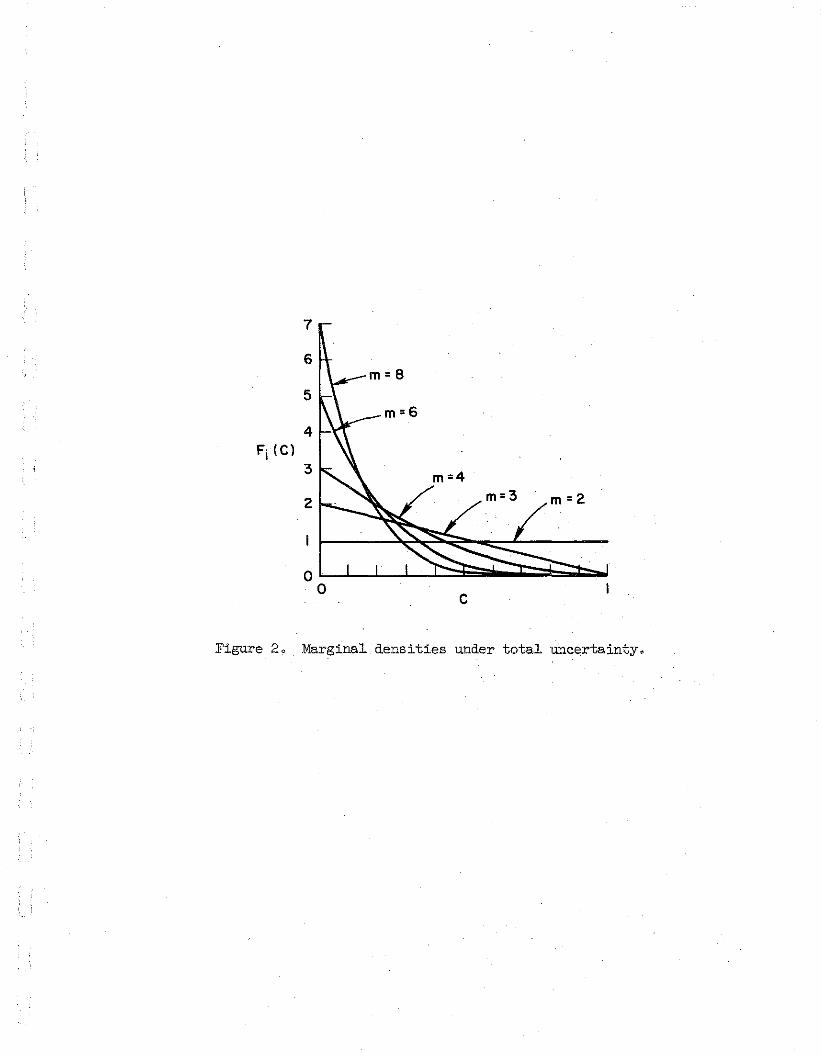
The results were a number of discrete values of F.(C) for eachl

particle and for each subject. For each particle we pooled the results

of the 10 subjects who were tested for each value of m. We then did a

standard analysis of variance test to ascertain whether any significant

differences existed in Ss' responses for the different particles.

As Table 1 shows, there were no significant differences among particles

at the .05 level.

Table 1 - Analysis of Variance on Differences Among Particles

Series df F Significance Level

m = 2 1/162 .10 p> .05

m = 4 3/324 .35 p> .05

m = 8 7/432 1.03 p> .05

What Table 1 indicates is that Ss accepted Laplace's principle

of insufficient reason; they showed no preference for any particular

particles. The Ss' answers to ~uestions after experimentation confirmed

this result. Since Ss accepted the principle of insufficient reason,

results were also pooled across particles. Figs. 3a, 3b, and 3c show

the nbrmative cumulatives F.(C) as well as our data points pooled acrossl

Ss and particles for each of the three different values of m. The

median responses shown in the figures correspond closely to the means.

28

Insert Figs. 3a, 3b, and 3c about here

Fig. 3a clearly indicates that for m = 2 the normative model fits

the data very well, whereas for m = 4 and m = 8 there is some relation

between the normative model and the data but not a fit.

The variance analysis of the data that is displayed in Table 2

indicates that when m = 2 there is no significant difference between

the normative curve and the data at the .05 level. For m = 4 and

m = 8 the difference between the normative curve and the data is

significant at the .001 level.

Table 2 ~ Analysis of Variance on Differences

between Normative Models and Data

Series df F Significance Level

m = 2 1/162 1.36 p> .05

m = 4 1/162 100·33 p < .001

m = 8 1/108 229·52 p < .001

Since the normative curves fit the data so poorly when m = 4

and m = 8, we decided to use a one-parameter curve of the same form as

the normative model and fit it to the data by least sQuares techniQues.

That is, we wished to describe the data by a curve of the following

nature:

F.*(C) = 1 - (1 _ C)m*-l.1

-' normative cumulative~ - descriptive cumulative

II st ,quartilemediall3rd quartile

(a)m=2

ollL-l....-l....-l....-l....-l....-L......JL......JL......J'--J

I

(b)

m=4

0

I -" I// I

11/ Ir/ (e)

I m=8

c

Figure 30 Normative and descriptive cumulatives for(a)m = 2, (p) m= 4, and (c) m = 80

29

*The * superscript indicates that Fi (C) and m* are descriptive

rather than normative. The least squares estimate. of m* is that

value of m* which minimizes the ~ given in equation (6).

where Cl ~ 25/100 , C2 ~ 100/1000, etc., and Pj,obs is the mean

probability estimate of the Ss. Table 3 shows the least squares

estimates of m* computed numerically on Stanford's IBM 7090.

Table " - Least Sauares Estimates of m*

(6)

Series

m ~ 2

m ~ 4

m ~ 8

, m*

1.98

2.63

4.05

.00

.04

Figs. 2b and 2c

Table 3.

*show F. (C)1

based on the values of m* given in

Our data indicate that Ss' beliefs are quite close to the

normative mOdel for m ~ 2, scarcely a surprising result. For m> 2

Ss' beliefs shift toward the normative model, but not sufficiently far.

The reason for this is suggested in Figs. 4a, 4b, and 4c where f. (C)1

*and. f i (C) are plotted. *(f. (C) is the descriptive density based on1

the value of m* given in Table 3 inserted into equation (4).)

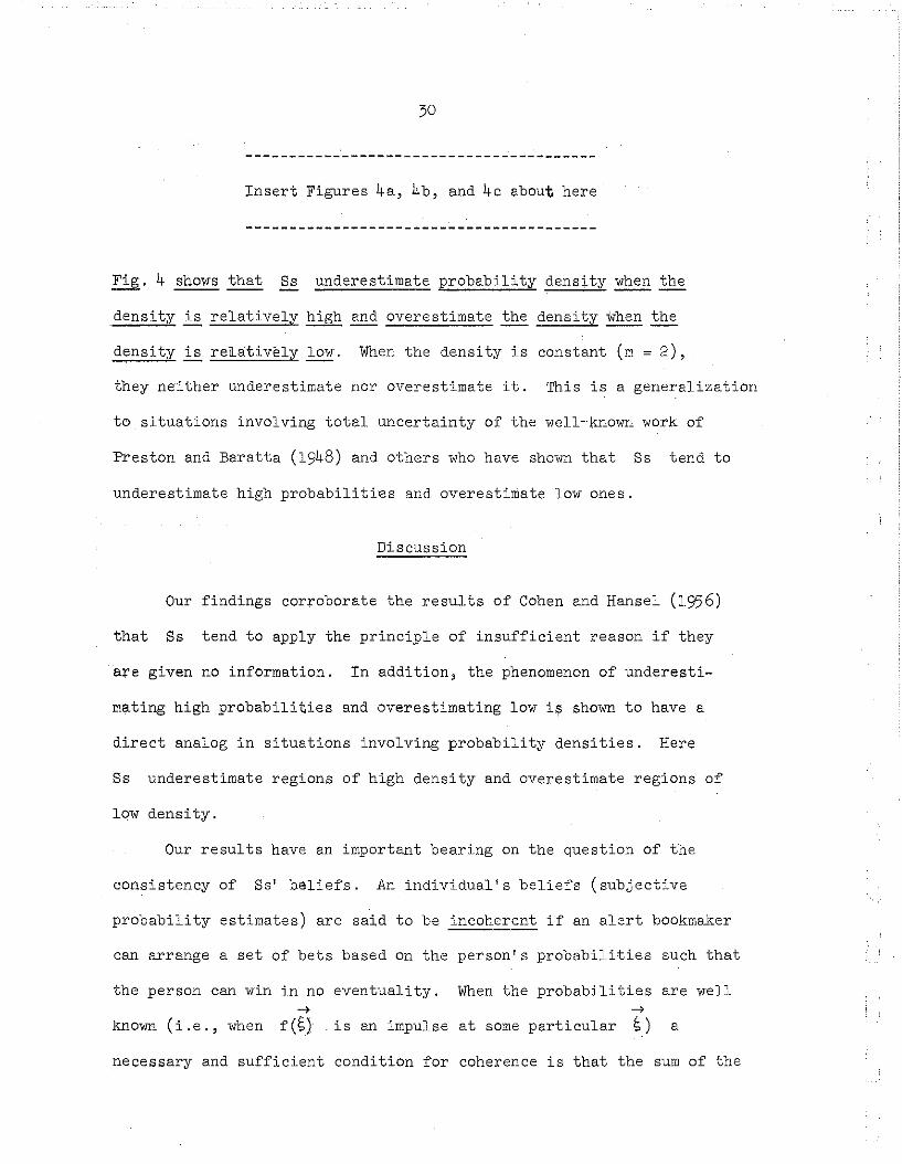
30

Insert Figures 4a, 4b, and 4c about here

Fig. 4 shows that Ss underestimate probability density when the

density is relatively high and overestimate the density when the

density is reiatively low. When the density is constant (m = 2),

they neither underestimate nor overestimate it. This is a generalization

to situations involving total uncertainty of the well-known work of

Preston and Baratta (1948) and others who have shown that Ss tend to

underestimate high probabilities and overestimate low ones.

Discussion

Our findings corroborate the results of Cohen and Hansel (1956)

that Ss tend to apply the principle of insufficient reason if they

are given no information. In addition, the phenomenon of underesti-

mating high probabilities and overestimating low is shown to have a

direct analog in situations involving probability densities. Here

Ss underestimate regions of high density and overestimate regions of

low density.

Our results have an important bearing on the Question of the

consistency of Ss' beliefs. An individual's beliefs (subjective

probability estimates) are said to be incoherent if an alert bookmaker

can arrange a set of bets based On the person's probabilities such that

the person can win in no eventuality. When the probabilities are well->

known (i.e., when f(S)->

is an impulse at some particular S) a

necessary and sufficient condition for coherence is that the sum of the

3

(a )m=2

2

03

( b)

m=42

fj Ie1

.... .........'" '"""0

,7

6 (c )

5 m=8

4

3 ---fjIC)

*2

--fj(C)

Figure 4. Normative and descriptive densities for(a) m ~ 2, (b) m ~ 4, and (c) m ~ 8.

31

probabilities of mutually exclusive and collectively exhaustive events

be unity (see.Shimony (1955)). Analogously, a necessary (but not

sUfficient) condition for coherence when probabilities are not well

known is that the sum of the expectations of the probabilities be

unity. That is, the R defined below must equal one.

m JlR = L: C f.(C)dC.i=l 0 l

Since all the f.s are equal (from the insignificance of the differencesl

among particles),

m= m*' (8)

Thus R = 1 only when m* = m. It is clear from Table 3 that when

m = 4 and m = 8, the Ss in our experiment had beliefs that were

strongly incoherent.

Our study is an exa~ination of the static structure of a person's

beliefs when he is in a situation of total uncertainty. The natural

extension of this work is to examine the kinematics of belief change

when the S is given information relevant to the situation. Work on

the kinematics of belief change when probabilities are well known is

reported in a number of papers in a volume edited by Edwards (1967).

32

Appendix

Instruction to Subjects

The instructions that were read to the Ss when m = 8 are given

below. The instructions for ill = 2 and m = 4 are the same except for

obvious modifications.

* * * * * * * *

We are running an experiment to examine the nature of a person's

intuitions concerning situations where he has little or no concrete

evidence to guide him. You will be asked to estimate the likelihood

of certain propositions concerning a hypothetical scientific experiment.

While there are no absolutely "right" or "wrong" answers, some answers

are better than others. Your response will be evaluated against a

hypothetical ideal subject.

Let me now describe the hypothetical scientific situation about

which we wish to examine your beliefs. A particle measuring device

is placed into an environment where there are 8 distinct types of

particles which we shall designate by letters of the Greek alphabet-­

~, E, W, 6, ~, E, X, e. What the particle measuring device does is

count the number of each type of particle that hits it in a given time

interval. We leave the counter in the environment until it has been

struck by a total of 1000 particles of the 8 types. Do you remember

what the 8 types were? Prior to the experiment you are assumed to have

absolutely no knowledge a.bout the relative numbers of the 8 types of

33

particles except that some of each may exist and that no other type of

particle is in the environment. Given this scant information, and

nothing else, we want to examine your intuitions concerning how many of

each type of particle will be included in the 1000 measured by the

detector.

The questions we ask you concerning your beliefs will be of the

, following form: What do you think the probability is that there are

less than some specific number Of, say, e-particles among the 1000

counted? This statement would be true, of course, if there were

0, 1, 2, 3, ... , or any number up to that number of e-particles among

those counted but it would not be true if there were more than that

many e-particles. What you are being asked is how likely is it that

there are less than that number of e-particlesZ If you believed that

there were certainly less than that number of e-particles, you would

tell us that the probability of there being less than that number is

If, on the other hand, you believed that there were certainly

more than that number of e-particles, you would tell us that the

probability that there is less than that lmmber';'is ..• '.:, If you

believe that it is equally likely that there are more than that number

as less, you would say the probability is .5. You can give us any

probabili ty between zero and one.

Perhaps a more concrete example will help make things clear.

Consider an ordinary die such as this one. What do you think the

probability is that if I roll this die a number less than 2 will be on

the upturned face? What do you think the probability is of less than

5? Clearly, the probability of less than 2 must be smaller than the

probability of less than 5. Well, you see, this is exactly the same

type of question that we shall be asking concerning particles cDunted

by our counter. The only difference is that with a die you already;

have a good idea of the probability asked for,whereas in this experiment

we are asking for your intuitions concerning unknown probabilities.

Let me now ask you a few sample questions before we begin. First,

what do you think the probability is that there are less than 1001

*-particles among those counted? [Explain if answer is wrong.] What

do you think the probability is that there are less than 950 W - particles

among the 1000 counted? Less than 75 E? Remembering, again, that there

are 8 types of particles, what do you think the probability is of less

than 500 E-particles? Less than 950 6-,? [No feedback is given on last

4 que stions. ]

In front of you is a stack of 3" x 5" cards that you will write

your replies on. Could you write your replies as a two-digit decimal

like so.

Before we begin, please feel free to ask any questions you might

have.

35

References

Atkinson, F., Church, J. &Harris, B. Decision procedures for finite

decision problems under complete ignorance. An~. Math.. Statist.,

1965, 35, 1644-1655.

Cohen, J. &Hansel, M. ~~ Gambling. London: Longmans Green,

Edwards, W. The theory of decision making. Psychol. Bull., 1954, 2'

280-417.

Edwards, W. (Ed.) Revision of opinions of men and man-machine systems.

Special issue of IEEE Trans. on Human Factors in Electron.,

1967, I, 1-63.

Jamison, D. Bayesian decisions under total and partial ignorance.

This technical report.

Luce, R. D. & Raiffa, H. Games and Decisions:---- Introduction and

Critical Survey. New York: John Wiley & Co., 1956.

Luce, R. D. & Suppes, P. Preference, utility, and subjective

probability. In R. Luce, R. Bush & E. Galanter (Eds.), Handb.

Math. Psychol., Vol. 3. New York: John Wiley & Co., 1965. Pp.

250-410.

Preston, M. G. & Baratta, P. An experimental study of the auction

value of an uncertain outcome. Amer.:L..Psychol., 1948, 61,

183-193.

Savage, L .. J. ~ .FPundations of' Statis tics. New York: John Wiley

& Co., 1954.

Shimony, A. Coherence and the axioms of confirmation. J. Symbolic

Logic, 1955, ~, 1-28.

36

Footnotes

1The work reported here was performed at the Institute for

Mathematical Studies in the Social Sciences, Stanford University. The

authors wish to thank the Institute's Director, Professor Patrick

Suppes, for his support of and helpful comments concerning this work.

Professor Richard Smallwood made some helpful comments on an early

draft of this paper.

2Luce and Raiffa (1956) review normative theories of decision

making under total uncertainty. Extensions of these other theories

may be found in Atkinson, Church, & Harris (1965). Savage (1954)

presents a number of objections to the probability of probabilities

approach used here. These alternatives and objections are all

discussed in Jamison (1967).