De Luca, F., Vamvatsikos, D., & Iervolino, I. (2013). Near-optimalpiecewise linear fits of static pushover capacity curves for equivalentSDOF analysis. Earthquake Engineering and Structural Dynamics,42(4), 523-543. https://doi.org/10.1002/eqe.2225

Peer reviewed version

Link to published version (if available):10.1002/eqe.2225

Link to publication record in Explore Bristol ResearchPDF-document

This is the peer reviewed version of the following article: De Luca, F., Vamvatsikos, D. and Iervolino, I. (2013),Near-optimal piecewise linear fits of static pushover capacity curves for equivalent SDOF analysis. EarthquakeEngng. Struct. Dyn., 42: 523–543, which has been published in final form at DOI: 10.1002/eqe.2225. This articlemay be used for non-commercial purposes in accordance with Wiley Terms and Conditions for Self-Archiving

University of Bristol - Explore Bristol ResearchGeneral rights

This document is made available in accordance with publisher policies. Please cite only thepublished version using the reference above. Full terms of use are available:http://www.bristol.ac.uk/red/research-policy/pure/user-guides/ebr-terms/

1

NEAR-OPTIMAL PIECEWISE LINEAR FITS OF STATIC PUSHOVER

CAPACITY CURVES FOR EQUIVALENT SDOF ANALYSIS*

F. De Luca,1†

D. Vamvatsikos2, I. Iervolino

1

1Department of Structural Engineering, DIST, University of Naples Federico II, Via Claudio,21,

80125 Napoli, Italy.

2School of Civil Engineering, National Technical University of Athens, 9 Heroon Polytechneiou,

15780 Athens, Greece.

Keywords: equivalent SDOF, piecewise linear fit, static pushover, incremental dynamic

analysis.

Abstract. The piecewise linear (“multilinear”) approximation of realistic force-deformation

capacity curves is investigated for structural systems incorporating generalized plastic, hard-

ening, and negative stiffness behaviors. This fitting process factually links capacity and de-

mand and lies at the core of nonlinear static assessment procedures. Despite codification, the

various fitting rules used can produce highly heterogeneous results for the same capacity

curve, especially for the highly-curved backbones resulting from the gradual plasticization or

the progressive failures of structural elements. To achieve an improved fit, the error intro-

duced by the approximation is quantified by studying it at the single-degree-of-freedom level,

thus avoiding any issues related to multi- versus single-degree-of-freedom realizations. In-

cremental Dynamic Analysis is employed to enable a direct comparison of the actual back-

bones versus their candidate piecewise linear approximations in terms of the spectral

acceleration capacity for a continuum of limit-states. In all cases, current code-based proce-

dures are found to be highly biased wherever widespread significant stiffness changes occur,

generally leading to very conservative estimates of performance. The practical rules deter-

mined allow, instead, the definition of standardized low-bias bilinear, trilinear, or

quadrilinear approximations, regardless of the details of the capacity curve shape.

1 INTRODUCTION

In the last decades, improvements in the computational capabilities of personal computers

have allowed the employment of nonlinear analysis methods in many earthquake engineering

problems. In this framework, nonlinear static analysis is becoming the routine approach for

the assessment of the seismic capacity of existing buildings. Consequently, nonlinear static

procedures (NSPs) for the evaluation of seismic performance, based on static pushover analy-

sis (SPO), have been codified for use in practice. Most of such approaches consist of the same

five basic steps: (a) perform static pushover analysis of the multi-degree-of-freedom (MDOF)

system to determine the base shear versus (e.g., roof) displacement response curve; (b) fit a

piecewise linear function (typically bilinear) to define period and backbone of an equivalent

single-degree-of-freedom system (SDOF); (c) use a pre-calibrated R--T (reduction factor –

ductility – period) relationship for the extracted piecewise linear backbone to obtain SDOF

seismic demand for a given spectrum; (d) translate the SDOF response to the MDOF “target

displacement” (usually at the roof level) and use the static pushover curve to extract MDOF

* Based on short papers presented at the 3rd International Conference on Computational Methods and Structural

Dynamics and Earthquake Engineering COMPDYN 2011, Corfu, Greece, 2011 and at the ANIDIS2011 Conven-

tion on Seismic Engineering, Bari, Italy. † Corresponding author: flavia.deluca@unina.it

2

response demands for the entire structure; (e) compare demands to capacities; see [1] for ex-

ample.

NSP is a conventional method without a rigorous theoretical foundation for application on

MDOF structures [2], as several approximations are involved in each of the above steps. On

the other hand, its main strength is that it provides an estimate of structural demand and ca-

pacity in a simple and straightforward way. Although several improvements and enhance-

ments have been proposed since its introduction, any increase in the accuracy of the method is

worth only if the corresponding computational effort does not increase disproportionately.

Extensively investigated issues are the choice of the pattern considered to progressively load

the structure and the implication of switching from the nonlinear analysis of an MDOF system

to the analysis of the equivalent SDOF sharing the same (or similar) capacity curve. Regard-

ing the shape of the force distributions, it was observed that an adaptive load pattern could

account for the differences between the initial elastic modal shape and the displacement shape

in the nonlinear range [3,4,5]. Contemporarily, other enhanced analysis methodologies were

proposed to account for higher mode effects and to improve the original MDOF-to-SDOF ap-

proximation [e.g., 6]. Regarding the demand side, efforts have been made to improve the es-

timation of the target displacement, especially by providing advanced R--T to better evaluate

the inelastic seismic performance at the SDOF level; e.g., [7,8]. A comprehensive investiga-

tion of many of these issues has recently appeared in the NIST GCR 10-917-9 [9] report.

One of the issues not yet systemically investigated is the approximation introduced by the

imperfect piecewise linear fit of the capacity curve for the equivalent SDOF. The necessity to

employ a multilinear fit (an inexact, yet common, expression to describe a single-variable

piecewise linear function) arises due to the use of pre-determined R--T relationships that

have been obtained for idealized systems with piecewise linear backbones. This has become

even more important recently since nonlinear modeling practice has progressed towards real-

istic member models, which may accurately capture the initial stiffness using uncracked sec-

tion properties and/or include in-cycle strength degradation. The gradual plasticization of such

realistic elements and models introduces a high curvature into the SPO curve that cannot be

easily represented by one or two linear segments. It is an important issue whose true effect is

often blurred, being lumped within the wider implications of using an equivalent SDOF ap-

proximation for an essentially MDOF system. Despite these limitations, some light has al-

ready been shed on this issue. For example recent studies have shown the influence of

accounting for uncracked stiffness in the structural response of reinforced concrete (RC)

structures [10], while others [9] have shown the importance of accurately capturing both the

pre- and post-cracking stiffness for RC shear wall structures; such studies already provide a

general idea on the phenomena that an optimal fit should be able to capture within conven-

tional NSP approaches to maintain accuracy.

To reach concrete solutions, the effect of the piecewise linear approximation will be inves-

tigated in stages, practically following the progression of modern R-μ-T relationships from the

simple bilinear to the more complex quadrilinear backbone shapes by adding one linear seg-

ment at a time. Thus, starting with an elastic segment, we will successively add a perfectly-

plastic or positive-stiffness “hardening” segment, a negative stiffness “softening” segment and

a low-strength zero-stiffness “residual” plateau. In essence, the optimal fitting of four differ-

ent shapes will be examined comprising (a) bilinear elastoplastic, (b) bilinear elastic-

hardening (c) trilinear elastic-hardening-negative and (d) quadrilinear elastic-hardening-

negative-residual. While the first two cases are typical in most NSP guidelines, e.g., [11,12],

the latter two have also become an option in recent codes (ASCE/SEI 41-06) [13,14], or lit-

erature [15,16].

The approach employed will be based on the accurate assessment of the effect of the ca-

pacity curve fit on the NSP results. This is achieved by proper quantification of the bias intro-

3

duced into the estimate of the seismic response at the level of the SDOF itself. Incremental

dynamic analysis (IDA) [17] will be used as the benchmark method to quantify the error in-

troduced by each candidate fit with respect to the exact capacity curve of the SDOF. Figure 1a

shows a typical example, where an elastoplastic backbone is fitted to a highly-curved SPO

shape according to the equal area criterion, i.e., by equalizing the area discrepancy above and

below the fitted curve. Such an approximation actually follows the Eurocode 8 (EC8) provi-

sions [11] and it is not far from the ASCE/SEI 41-06 [13] guidelines for a target displacement

deep within the plastic plateau. The corresponding median IDA curves displayed in Figure 1b

in terms of spectral acceleration (the intensity measure, or IM) versus displacement (the engi-

neering demand parameter, or EDP) show that the fitted backbone produces nearly 25% high-

er displacement demand at all intensity levels. Thus, even code-mandated fitting rules may

lead to an unintended hidden bias that will be shown to be generally conservative but may of-

ten become unreasonably high.

In the sections to follow the methodology considered will be fleshed out and applied to

quantify the approximation errors. By extensive investigation of numerous candidate piece-

wise linear fits, a set of fitting rules will be established that can offer a standardized near-

optimal capacity curve approximation, suitable for immediate application in NSPs with supe-

rior performance compared to fitting approaches currently in use.

Figure 1. (a) Example of exact capacity curve versus its elastoplastic bilinear fit according to EC8 and (b) the

corresponding median IDA curves showing the negative (conservative) bias due to fitting for T=0.5s.

2 METHODOLOGY

The main target is the quantification of the error introduced in the NSP-based seismic perfor-

mance assessment by the replacement of the original capacity curve of the system, termed the

“exact” or “curved” backbone, with a piecewise linear approximation, i.e., the “fitted” or “ap-

proximate” curve (e.g., Figure 1a). This will enable a reliable comparison between different

fitting schemes in an attempt to minimize the observed discrepancy between actual and esti-

mated performance. In all cases, to achieve an accurate and focused comparison of the effect

of fitting only, it is necessary to disaggregate the error generated by the fit from the effect of

approximating an MDOF structure via an SDOF system. Thus, all the investigations are car-

ried out entirely at the SDOF level, using a variety of capacity curve shapes, different periods

and hysteresis rules and using IDA as the method of choice for assessing the actual perfor-

mance of the different alternatives. Such an approach is meant to single out a near-optimal fit

that can be directly included in current NSP procedures.

2.1 Exact versus approximate SDOF systems

An ensemble of SDOF oscillators is considered with varying curved shapes of force-

deformation backbones. Their strength and stiffness is essentially provided by bundling to-

gether multiple uniaxial springs in parallel (i.e. a fiber section), each with its own bilinear,

4

trilinear, or quadrilinear capacity curve but having the same general hysteretic (cyclic) behav-

ior. The first part of the investigation addresses non-softening behaviors; the backbones, in

fact, display a monotonically decreasing stiffness that starts from its elastic value and de-

grades with increasing displacement to reach a final zero or positive stiffness that remains

constant afterwards (e.g., Figure 1a). According to their final constant stiffness, these will be

termed “generalized elastoplastic” and “generalized elastic-hardening” systems, respectively.

They are all fitted accordingly with bilinear elastoplastic or elastic-hardening shapes. The se-

cond part of the investigation focuses on backbones displaying negative stiffness, i.e., soften-

ing, termed “generalized elastic-hardening-negative” systems. First the use of an elastoplastic

fit that is extended beyond the peak of the backbone to take into account the early negative

slope will be investigated (e.g., as recommended by the current Italian building code [18]).

Then, the higher fidelity three- or four-segment piecewise linear fit for backbones with non-

trivial softening behavior, will be addressed.

For each considered curved backbone shape, 5% of critical viscous damping was used and

appropriate masses were employed to obtain a range of matching “reference” periods of 0.2,

0.5, 1 and 2 seconds. The concept of the “reference” period, instead of the actual initial (tan-

gent at zero displacement) period, is introduced because of the highly curved shape of some

backbones. In some cases the backbones show a strictly localized significant change in the

initial stiffness, resulting in periods lower than 0.01s. Since this initial stiffness disappears

almost immediately for any kind of loading history, a more representative reference period is

required for each exact (curved) capacity curve. The reference period (T herein) was defined

as the secant period at 2% of the displacement corresponding to the peak force capacity.

Actually, in the vast majority of the cases there was insignificant difference between the

initial tangent period and the reference secant period. In all cases, both the exact and the ap-

proximate system share the same mass, but, due to the typically lower initial stiffness of the

latter, the “equivalent” period of the fitted curve tends to be higher than the “reference” one,

thus replicating the approach followed in the conventional NSP methodology [1]. In addition,

it is assumed that the backbone curve itself suffices to capture via its shape all the in-cycle

degradation effects (e.g., due to material nonlinearity, P-Delta effects, etc.) without needing to

use approximate coefficients (FEMA-356 [12]) or two separate analyses with and without P-

Delta (FEMA-440 [14]).

In order to draw general conclusions that are independent of the cyclic hysteretic behavior

assumed, two distinct cyclic hysteretic rules were initially considered for each curved back-

bone and its fit. The first is a standard kinematic strain hardening model without any cyclic

degradation characteristics. The second is a pinching hysteresis featuring cyclic stiffness deg-

radation [19]. In all cases, when comparing an original system with its approximate having a

piecewise linear backbone, the same hysteretic rules are always employed, so that both sys-

tems display the same characteristics when unloading and reloading in time-history analyses.

In other words, all differences observed in the comparisons to follow can be attributed to the

fitted shape of the approximate backbone, obviously also capturing any differences due to

mismatches between the exact (“reference”), in the following always referred to as T, and the

“equivalent” oscillator period.

When working with the backbone shapes and their fits it is useful to avoid the appearance

of arbitrary scales and units of force F or displacement δ. Thus, using the normalized counter-

parts, Fn and δn, becomes attractive. Unfortunately, the concise definition of a yield point on

curved (exact) backbones is impractical, unless tied to some preselected fitting rules; therefore

it is not possible to use a strength reduction factor, or equivalent ductility, without bias. In-

stead, it was chosen to uniformly normalize force and displacement by the reference values of

1kN and 0.10m, respectively. These values correspond to the point where the generalized

elastic-plastic backbones reach their plastic plateau (e.g. Figure 1a) by becoming fully plasti-

5

cized. More complex backbone curves have been generated building upon the elastoplastic

ones in a consistent manner; i.e., by replacing the individual bilinear uniaxial springs forming

the overall SDOF system with trilinear or quadrilinear ones sharing the same yield points.

Thus, the above reference values generally represent a point in the “hardening” region, be-

tween near-elastic behavior and peak strength, where a nominal yield point would normally

reside.

For each exact shape of the SDOF’s capacity curve and for each period value, several

piecewise linear fit approximations have been considered according to different fitting rules.

These include typical code-suggested fits, e.g., as laid out in Eurocode 8 [11], FEMA-356

[12], ASCE/SEI 41-06 [13], and the Italian Code (Circolare 617/2009, [18]). In addition sev-

eral bilinear, trilinear and quadrilinear fits, including solutions available in literature

[15,16,20], have been investigated. Different fitting criteria, e.g., varying initial stiffness,

yield point definition, and softening slope, have been employed in an attempt to pinpoint the

consistent characteristics that can define an optimal or near-optimal fit. In all cases, the aim is

to provide a standardized approximation that delivers accuracy yet remains largely independ-

ent of the NSP target displacement, to offer a single representation of the static pushover

curve for a wide range of limit-states considered. Choosing among such candidate fits neces-

sitates a precise comparison on the basis of their nonlinear dynamic response. Thus, as men-

tioned, IDA will be employed.

2.2 Performance-based comparison via IDA

IDA is arguably the most comprehensive analysis method available for determining the

seismic performance of structures. It involves performing a series of nonlinear dynamic anal-

yses by scaling a suite of ground motion records to several levels of intensity, characterized

by a scalar IM, and recording the structural response via one or more EDPs. The results typi-

cally appear in terms of multiple IDA curves, one for each record, plotted in the IM versus

EDP space. These can be in turn summarized into the 16, 50, 84% fractile curves of EDP giv-

en IM (EDP|IM) or, equivalently [21], as the practically identical 84, 50, 16% fractile curves

of IM given EDP (IM|EDP). The summarized curves, thus, provide the (central value and the

dispersion of the) distribution of EDP seismic demand given the IM intensity of the earth-

quake or, vice-versa, the distribution of a structure’s IM-capacity that a ground motion’s in-

tensity should reach to achieve the given value of EDP response.

To perform IDA for each exact and approximate oscillator considered, a suite of sixty

ground motion records was used, comprising both horizontal components from thirty record-

ings from the PEER database [22]. They are all characterized by relatively large moment

magnitude (between 6.5÷6.9) and moderate distances of the recording site from the source

(15km÷35km), all recorded on firm soil and bearing no marks of directivity. Using the hunt &

fill algorithm [21], 34 runs were performed, per record, to capture each IDA curve with excel-

lent accuracy. The IM of choice was Sa(τ), the 5%-damped elastic spectral acceleration at the

period τ of the oscillator, this being the reference period for the exact systems or the equiva-

lent for the fitted ones. The oscillator displacement δ (or its normalized counterpart δn) was

used as the corresponding EDP, being the only SDOF response of interest for NSP.

Once the IM and EDP are decided, spline or linear interpolation [21] allows the generation

of a continuous IDA curve from the discrete points obtained by the 34 dynamic analyses for

each ground motion record. The resulting sixty IDA curves can then be employed to estimate

the summarized IDA curves for each exact and approximate pair of systems considered. Still,

in order to be able to compare an exact system with reference period T with its approximation

having an equivalent period Teq, it was necessary to have their summarized IDA curves ex-

pressed in the same IM. In this case it is chosen to be Sa(T), i.e., the spectral ordinate at the

reference period of the curved (exact) backbone oscillator. Thus, while the approximate sys-

6

tem IDA curves are first estimated as curves in the Sa(Teq) – δ (or δn) plane, they are then

transformed to appear on Sa(T) – δ axes. This is achieved on a record-by-record basis by mul-

tiplying all 34 Sa(Teq) values comprising the i-th IDA curve (i=1,2,…,60) by the constant

spectral ratio [Sa(T)/Sa(Teq)]i that characterizes the i-th record [23].

The error is evaluated for every value of displacement in terms of the relative difference

between the two systems’ median Sa-capacities, both evaluated at the reference period T of the

exact system:

)(

)()()(

50,

50,50,

50

n

exact

a

n

exact

an

fit

a

nS

SSe

(1)

Alternatively, one could use the relative error in the median displacement response given the

level of spectral acceleration:

)(

)()()(

,

,,

aexact

n

aexact

nafit

na S

SSSe

50

5050

50

(2)

Similarly, the same definitions can be used to estimate the errors for different demand or

capacity fractile values, e.g., 16% or 84%, or even for the dispersion in response or capacity,

which, assuming lognormality, can be defined as one half the difference between the corre-

sponding 84% and 16% values. Thus, two different ways of measuring the discrepancy be-

tween IDA curves are available, e.g., for the two median IDA curves shown in Figure 1b. In

one case “horizontal statistics” are employed, working with the median EDP given IM, and in

the other case “vertical statistics” of IM given EDP (with compliments to Professor H.

Krawinkler for these very descriptive terms). As Vamvatsikos and Cornell [21] have shown,

the median IDA curve is virtually the same, regardless of how it is calculated, while, as dis-

cussed earlier, the 16, 84% fractiles are simply flipped. In addition, while there might be dif-

ferences in the error estimates using these two different methods, they are only an issue of

scale. Figures 2a, 2b compare the two error quantification methods for the median IDAs

shown in Figure 1b (an example of generalized elastic-plastic behavior). The observed trends

are actually the same, but simply inverted: obviously, an overestimation in response becomes

an underestimation in capacity and vice-versa.

Figure 2. The mean relative error in the median capacity (black line) shown against the overall average (grey line)

as introduced by the bilinear fit in Figure 1a. It is expressed on the basis of (a) response given intensity (EDP|IM)

and (b) intensity given response (IM|EDP).

Why then should one method be preferred over the other? There are three important rea-

sons that make the IM-based method (IM|EDP) a more attractive solution. First, parameteriz-

ing the error in terms of the displacement response simplifies its visualization since

displacement is directly mapped to specific regions of the oscillator force-deformation back-

bone. Thus, it is possible to see directly in Figure 2b, when it is compared vis-à-vis Figure 1a,

7

whether it is the “elastic” or the “post-elastic” part that is causing the accumulation of error.

Figure 2a is much more difficult to understand, especially if more complex backbones, than

the ones used here, are considered. Second, comparing the exact versus the fitted equivalent

system on the basis of Sa-capacity, links directly to comparison in terms of seismic perfor-

mance, as expressed by the mean annual frequency (MAF) of violating limit-states defined by

the oscillator displacement [24]. An over/under-estimation of Sa-capacity maps to a consistent

(although not commensurable) under/over-estimation of the MAF of limit-state exceedance,

provided that the difference between the reference and the equivalent period is not overly

large. Finally, when collapse enters the problem it is obvious that the error in displacement

may easily diverge when, at a given intensity level, one system has collapsed, while the other

has not. On the contrary, this is never a problem for the Sa-based error. These are all compel-

ling reasons to recommend only the Sa-based comparison for general use.

As a final note, it should be stated that when applying to actual NSP, there are many fac-

tors that will determine the final error. Thus, the error found herein, either represented in Sa or

in displacement terms, is only indicative of the magnitude of the overall error that would be

observed in NSP of a given structure. Other details, based on the nature of the structure itself

will often matter more. Still, the error estimated here is an accurate measure of the quality of

the fit itself, and it will allow selecting the one that best fits any given backbone curve and

minimizes the contribution of this source of error to the overall results.

3 BILINEAR FITS FOR NON-SOFTENING BEHAVIOR

Bilinear elastic-plastic or elastic-hardening fits are the fundamental force-deformation approx-

imations employed in NSP guidelines. The simplicity of the bilinear shape means that the on-

ly need is to estimate the position of the nominal “yield point” and select a value for the

constant post-elastic stiffness. Eurocode 8 [11], following the original N2 method [1], sug-

gests an elastic-plastic idealized backbone based on the balancing of the area discrepancy

above and below the fit, optionally using an iterative procedure. FEMA documents [12,14]

generally employ a bilinear elastic-hardening curve up to the target point. While a third sof-

tening segment was also considered indirectly by FEMA-356 [11], for demand estimation,

FEMA-440 [13] and consequently ASCE/SEI 41-06 [12] only use it to limit the allowable

value of the R-factor to protect against global collapse. In all cases, the idealized elastic-

hardening shape is fitted through an iterative procedure: the nominal yield point and the post-

yield slope are selected to achieve a balance of the misfit areas above and below the capacity

curve up to the target displacement, while also requiring that the elastic segment remains se-

cant at 60% of the nominal yield strength.

In order to develop an improved bilinear fit, the fitting of the initial “elastic” segment is

investigated separately and then the post-elastic non-negative stiffness part is added. General-

ized elastic-plastic systems will be first studied, where the stiffness becomes zero beyond a

displacement of 0.10 m, followed by generalized elastic-hardening backbones were the post-

yield stiffness is positive. In all cases the target is developing a standardized fitting rule that

performs well for a continuum of limit-states in the non-negative stiffness region.

3.1 Elastic-plastic fits

First, elastoplastic bilinear fits are considered for a family of generalized elastic-plastic ca-

pacity curves that exhibit a stiffness gradually decreasing with deformation, starting from the

initial elastic and reaching zero slope. The shapes are mainly characterized by the rate and

magnitude of the changes in stiffness with increasing displacement. Figure 3a and 3b give an

example of the shapes employed and emphasize two opposing cases. The first (Figure 3a) is

not characterized by significant curvature, while the second (Figure 3b) shows a significant

change in slope that can be representative of the behavior of a model that accounts for

8

uncracked stiffness (e.g., for RC or masonry structures) or displays progressive yielding of

elements.

Figure 3. Comparison of generalized elastic-plastic capacity curves and their corresponding fits having (a) insig-

nificant versus (b) significant changes in initial stiffness. Note: 0.1m displacement becomes 1.0 normalized.

Figure 4. The relative error in the median Sa-capacity of the 10%, 60% and equal area fits, when applied to the

capacity curves of Figure 3: (a)&(c) insignificant versus (b)&(d) significant changes in initial stiffness.

Three basic fitting rules are compared: (a) the “FEMA-style” fit (60% fit), (b) the “EC8-

style” fit using a simple area-balancing criterion (equal area), and (c) the 10% fit, defined so

that the intersection between the capacity curve and the fitted elastic segment is at 10% (in-

stead of 60% for the “FEMA-style” fit) of the maximum base shear. The latter is a simple

standardized rule that has been derived from extensive testing to better (near-optimally) cap-

ture the early seismic behavior. In all three cases the post-yield linear segment is chosen to

match the exact plastic-plateau. Strictly speaking this marks a slight deviation from the actual

FEMA fit which stipulates a variable post-elastic segment depending upon the target dis-

placement and the area-balancing rule. Still, our approach may be thought of being repre-

sentative of the code-mandated fit for a target displacement deep into the plastic plateau.

9

Figure 3a shows that when the capacity curves are not characterized by significant stiffness

changes, the three fits are very similar to each other. They differ significantly, though, when

the initial stiffness diminishes rapidly, as in Figure 3b. To investigate the differences between

the three fitting rules when applied to the two different backbones, IDA is performed for each

of the actual and approximate SDOF systems for a range of periods. Figures 4 show the com-

parison in terms of the normalized difference in the median Sa-capacity (Eq. 1) for T equal to

0.2 and 1.0 s. Obviously, the shape of the original backbone has a significant impact. In all

cases, the error increases with curvature while its maximum always appears at the earlier

backbone segments. Curiously, the 10% fit leads to a remarkable decrease in the error for any

deformation level, even for the highly curved shape of Figure 3b where it clearly violates any

notion of equal area (or equal energy) that seems to be prevalent in current guidelines. It leads

to a slightly non-conservative estimation of the capacity for displacements before the full

plasticization (for δn up to 1) and only for short-period systems, T = 0.2 s. In addition, even in

case of highly-curved backbones (Figure 4b) only a 10% underestimation appears at most.

Conversely, code approaches are always conservative for all the displacement levels and all

the shapes considered, but at a cost of almost 20%÷40% underestimation of capacity when

high curvature is present. The trends identified are generally confirmed for all other periods

considered. As noted previously, such conclusions are mirrored when operating on demands

(e.g., via Eq. 2) rather than capacities. Thus, for example, code fits are found to cause a signif-

icant (conservative) overestimation of displacement demand at all levels of intensity in com-

parison to the near-optimal 10% fit.

Figure 5. (a) Monotonic backbones and (b) the two hysteretic rules considered for the generalized elastic-plastic

systems, resulting in a sample of ten generalized elastic-plastic systems.

To verify the above observations, a sample of five different generalized elastic-plastic

shapes (see Figure 5a) was also considered for each of the two hysteretic rules described in

section 2, and shown in Figure 5b. Figure 6 display the statistics of the relative error on the

median Sa-capacity evaluated at T = 0.2s and 1.0s for the proposed 10% fit versus the conven-

tional FEMA-style 60% fit. The bias (computed on median response) is evaluated up to n = 2

(roughly a ductility of 2), where most of the significant differences appear. The cyclic hyster-

etic rules were found to be relatively insignificant, as the magnitude of the error depends pri-

marily on the shape of the fitted backbone (see also [15]); this result has also been confirmed

for other types of backbones and essentially frees us from the problem of having a hysteresis-

dependent optimal fit. Hysteresis aside, all the previously drawn conclusions are confirmed.

The 10% fit enjoys an insignificant bias, on average, for all the periods considered and its er-

ror never exceeds 20%. FEMA-style fits (60% fit), and similarly EC8-style approximations,

again show a strictly negative; i.e., conservative, bias of 20% or even 60%, depending on the

shape of the original backbone, most of which is concentrated at the low displacement range.

10

However, if the target displacement falls in this region, a strict application of the code guide-

lines would reduce the latter effect as they call for a more localized fit.

Figure 6. The relative error in the median Sa-capacity for the 10% and 60% fit, for a reference period of T = 0.2s,

1.0s, computed for ten generalized elastic-plastic systems, represented by the grey dotted lines.

The above stated results must still be viewed with caution whenever the equivalent “fitted”

and the reference “exact” period (T) differ significantly [24]. Since the 10% rule, by nature,

maintains a close match to the actual period, our conclusions regarding its excellent perfor-

mance remain robust. On the other hand, the code-based fits may result to disproportionately

large equivalent periods for highly-curved backbones. Then, the results of a more accurate

MAF-based performance comparison might differ from the Sa-based results discussed above

depending on the nature of the seismic hazard. Actually, it is possible that employing a code-

based fit for NSP assessment may prove to be unconservative due to this effect. For example,

if using a uniform-hazard spectrum with significant differences between short and long-period

hazard, the 20%÷40% conservative bias predicted earlier can be nullified or reversed. This

restriction should be kept in mind for all comparisons in the following sections.

Error comparisons for the Sa-capacity (record to record) dispersion are not shown as all fits

generally achieve equally good estimates. Of course, differences appear in the region preced-

ing the nominal yield point of each approximation. Therein the fitted system will predict no

dispersion, being essentially elastic and perfectly predicted by Sa, whereas the actual one

shows some small variability due to early inelasticity. This is to be expected and it cannot

weigh in favor of one fit over another.

Summing up, it can be stated that capturing the initial stiffness of the actual backbone is of

primary importance, as suggested also by [9,10]. Existing guidelines fail to achieve this for

highly curved backbones, leading to biased results that may become overly conservative.

Thus, the optimal fit should capture, as close as possible, the initial stiffness of the backbone,

being careful to avoid unreasonable estimates for initially ultra-stiff systems that quickly lose

11

their initial properties. Thus, fitting the “elastic” secant at 5% or 10% of the maximum base

shear, as opposed to 0.5% or 1%, is considered a robust strategy that delivers excellent results.

Despite solid numerical verification, the above findings viewed against Figure 3b may be-

come puzzling as the near-optimal fit does not resemble the curved backbone. This seems to

violate a fundamental “rule”, where fitting should be “close” to be accurate. In spite of our

findings above, such intuition is not in danger. As results show (e.g., see also [9], App.C),

when using more than two linear segments to fit the non-negative curved backbone, then in-

deed higher fidelity in capturing the backbone shape is possible and the accuracy increases, as

long as the initial stiffness (and period) is sufficiently represented. Thus, when utilizing better

and better discretization, things become indeed consistent with our current views: being closer

to the actual curve works best. The problems appear when working with a limited set of linear

segments; the indiscriminate use of area-balancing leads us to believe that the “area under the

curve” holds the same meaning for an elastic, a hardening or (later on) a softening segment. In

particular, the reason why the 60% fit is inferior to the 10% fit (e.g., Figure 3b) is simply be-

cause misrepresenting the initial stiffness has very important implications for seismic re-

sponse; much more important than misrepresenting the total area under the curve, as the 10%

fit does. Therefore, the proposed near-optimal fitting rules are simply a product of compro-

mise driven by the fact that R-μ-T relationships currently exist only for simple shapes.

3.2 Elastic-hardening fits

The second type of approximation investigated is the bilinear elastic-hardening fit for a

family of shapes characterized by a generalized elastic-hardening behavior. Only the pinching

hysteretic rule was considered, given the insignificant differences observed earlier when com-

pared to the kinematic hardening. Each backbone investigated is characterized by different

curvatures and final hardening stiffness, allowing a wide coverage of the typical shapes that

can be obtained considering different structural behaviors and modeling options.

When attempting to fit such shapes by a bilinear, determining the post-yield segment often

involves some kind of optimization to better fit the curved shape. Guidelines, such as EC8 [11]

or ASCE-41 [13] prescribe the graphical method of balancing the area discrepancy above and

below the fitted line, or, equivalently, of balancing the area enclosed by the fitted with the ar-

ea enclosed by the exact curve. While easy to apply graphically, area-balancing is an ill-

defined criterion that can yield mixed results: consider two coincident linear segments where

one, the “approximation”, is rotated by an arbitrary angle (other than 90o) around the common

center (Figure 7). Obviously, the rotated segment always satisfies the area balancing rule as a

valid approximation to the original. This is rarely a problem when applying by hand, as engi-

neers will intentionally make sure that the fitted curve is also close to the exact by minimizing

the absolute area discrepancy between the curves as well. Actually, pure area minimization

practically leads to the same result as the typical engineering approach above. In the thought

experiment of Figure 7, it produces a single solution, as the absolute discrepancy is A + A =

2A and it becomes zero only when the fitted coincides with the exact segment. Thus, area

minimization is algorithmically and mathematically superior and it will be our optimization

criterion of choice for all discussions that follow.

In analogy with the previous subsection, two different backbones will be presented in de-

tail. The first (Figure 8a) is characterized by mild changes in the oscillator stiffness, in con-

trast to the second (Figure 8b). The target displacement is assumed to be equal to 0.2m. The

EC8 fit is not applied as it is restricted to elastic-plastic approximations which are clearly in-

ferior for the shapes shown in Figure 8. On the other hand, the “FEMA fit” rule can be ap-

plied without problems, although, strictly speaking it might call for slightly different

approximations depending on the value of the target displacement. Still, the results and the

corresponding conclusions remain the same in all cases. The alternative fit proposed, based on

12

the 10% rule, determines the initial stiffness at 10% (instead of 60%) of the nominal yield

shear defined in accordance with FEMA, while the post-elastic stiffness is determined by

minimizing the absolute area discrepancy between the capacity curve and the fitted line. In

total, the proposed rule came out as the simplest standardizable rule with a near-minimum er-

ror for this family of backbones. In fact, while many other alternatives were considered, they

are not shown for the sake of brevity. It suffices to say that capturing the initial stiffness by a

secant in the range of 5%÷10% of the peak strength (or the nominal yield point) remains the

most important aspect of any successful fit. The definition of the nominal yield point is made

according to FEMA [12–14] provisions, thus the imposed intersection at 10% in alternative to

the suggested 60% and the use of area-minimization represent the only differences with the

codified approach.

Figure 7. There is an infinite number of “fitted” segments that will satisfy the area-balancing rule as “valid” ap-

proximations of the exact horizontal segment, as the area discrepancy is always A – A = 0.

Figure 8. Comparison of generalized elastic-hardening capacity curves and their corresponding fits having (a)

insignificant versus (b) significant changes in initial stiffness. Note: 0.2m displacement becomes 2.0 normalized.

The results of the proposed and the FEMA fitting procedures applied to the example

shapes appear in Figure 8. Obviously, when the stiffness of the backbone is not characterized

by abrupt changes in the curvature (Figure 8a) both fits tend to be practically the same. Figure

9 show the error introduced by each fit, for both backbone shapes considered in Figure 8, in

the cases of T = 0.2 and 1.0 s. In analogy with the results presented for the elastic-plastic case,

most of the error is concentrated at the beginning of the backbone. For low changes in the

stiffness (low curvature), it can be observed that the error is negligible for both fits, while it

becomes substantial for higher curvatures. In this case, the error introduced by the 60% fit

misrepresenting the initial stiffness is propagated throughout the results, even to displace-

ments deep in the nonlinear range, proving our statement that the area under the curve does

not hold the same importance everywhere. Capturing the initial stiffness is the key issue in the

fitting procedure, while the fitted hardening segment is an additional improvement. In fact,

replacing the hardening segment with a plastic plateau intersecting the actual backbone at the

13

target displacement (in this case 0.2 m) gave quite satisfactory results, at least for the cases at

hand.

For further verification a family of four different shapes is considered, shown in Figure 10a

where only the pinching hysteretic rule is used (Figure 10b). In Figure 11 the relative errors in

the median Sa-capacity, are compared for T = 0.2s, 1.0s. Again, the proposed fit leads to a

small and relatively unbiased error, which seldom exceeds 10%. In this case the sample of

backbones considered for the elastic-hardening case was smaller than the elastic-plastic case,

but the robustness of the general results, showing the same trends in both cases, supports the

remarks.

Figure 9. The relative error in the median Sa-capacity of the “FEMA fit” and 10% fit, when applied to the capac-

ity curves of Figure 8: (a)&(c) insignificant versus (b)&(d) significant changes in initial stiffness.

Figure 10. (a) The backbones and (b) the hysteretic rule considered for the generalized elastic-hardening systems.

It should be noted that the results of the FEMA approximation will improve if we refit ap-

propriately for each target displacement. Figure 12a presents such an example for the

elastoplastic backbone of Figure 3b, where both the FEMA fit and the proposed 10% fit are

compared by applying them not once for the entire curve but rather refitting them for each

14

target point separately over the range of 0 to 0.4m (or 0 to 4 in normalized terms). Two fit ex-

amples are provided for each fit rule in Figure 12a. From the error results in Figure 12b (in

which dots represents the errors at the target displacement for the two fitting rules), it be-

comes obvious that while both of the rules benefit by a custom-made fit, the proposed rule

retains its edge, typically halving the error of the FEMA fit.

Figure 11. The relative error in the median Sa-capacity the 10% fit and “FEMA fit”, for a reference period of T =

0.2s, 1.0s, computed for ten generalized elastic-hardening systems, represented by the grey dotted lines.

Figure 12. (a) A sample of alternate fits for target displacements of 0.1 and 0.4m. (b) The fitting error for a

properly executed FEMA-fit [12,13] versus the proposed 10% fit for a reference period of T = 1.0s for target

displacements up to 0.4m (4.0 normalized).

4 MULTILINEAR FITS FOR SOFTENING BEHAVIOR

Fitting the negative stiffness part of the static pushover curve has lately become an option

in NSP. In some cases (e.g., Italian provisions [18]) an elastoplastic fit is simply extended to

cover some portion of the early negative stiffness range while in others (e.g. FEMA-440 [14])

15

an additional negative stiffness linear segment is utilized. Until fairly recently, the negative-

stiffness segment was typically employed only indirectly either to achieve demand modifica-

tion (FEMA-356 [12]) or to set a limit on the allowable R-factor (ASCE/SEI 41-06 [12],

FEMA-440 [13]) due to the lack of appropriate R-μ-T relationships. With the emergence of

SPO2IDA, a set of R-μ-T expressions that can provide the distribution of nonlinear dynamic

response for complex SDOF systems [15], it is now possible to achieve for the entire range of

displacements, up to and including collapse, direct seismic demand and capacity estimation

for trilinear or quadrilinear backbone approximations that include negative stiffness.

4.1 Extended elastoplastic fits for generalized elastic-hardening-negative systems

The recent Italian seismic code [18] suggests that elastoplastic systems with extended

plateaus may be used to capture negative-stiffness behaviors up to a 15% loss of the peak base

shear capacity. Specifically, the Italian code is essentially a derivative of the FEMA-356 [12]

rule where a 60%-secant defines the initial stiffness and an area-balancing criterion is used to

get the plastic plateau which may now be extended into the negative stiffness range. Obvious-

ly, the yield strength of such a fit is always lower than the peak strength of the exact backbone.

To verify the feasibility of such an approach a direct search was undertaken by investigat-

ing an array of combinations of different plateau levels and “elastic” secant values in search

of the optimal solution. Out of the large number of candidate fits tried, only four will be

showcased (Figure 13a) on a highly-curved backbone out of a family of twelve (Figure 13b).

The initial stiffness is set at 10% or 60% of nominal yield strength combined with two plateau

levels at 80% (L) or 100% (H) of peak shear strength respectively. The corresponding candi-

date rules are named 10%L, 10%H, 60%L and 60%H, and their performance is shown in Fig-

ure 14a and 14b for 0.2s and 1.0s, respectively. Results show that capturing the initial part of

the backbone is still important, as the 10% fit maintains a consistently low-bias whenever

there are significant curvature changes in the exact backbone. Furthermore, foregoing any no-

tions of area-minimization or balancing to match the peak point instead (H versus L fits), is

always beneficial. The Italian fit rule will always have a plateau height between 80% and

100% therefore it displays a performance right between the 60%H and 60%L cases, in general

showing a 20%÷40% conservative bias. While only the results for pinching hysteresis are

shown herein, our conclusions persist if kinematic strain is employed instead.

Figure 13. (a) An example of generalized elastic-hardening-negative capacity curve having significant changes

in initial stiffness and its corresponding fits, (b) the backbones considered for the generalized elastic-hardening-

negative system sample.

The sample family of twelve backbones, selected for their diversity of shape (Figure 13b)

was also tested for the two opposing rules of 60%L and 10%H. Figure 15 display the relative

median Sa-capacity errors plotted against a displacement axis that has been normalized for

each backbone separately to ensure that the peak (p) and the ultimate (u) displacement points

16

are aligned. The results verify that the 10%H fit is an unbiased approach with robust perfor-

mance, at least up to the point where the structure loses about 20% of its maximum strength.

Consequently, it makes sense to suggest that an optimized rule should forego any strict area-

minimization (or balancing) considerations in favor of accurately capturing the maximum

base shear strength. Failing to follow this approach, the Italian code rule was, again, found to

be generally conservative, in analogy with other code fits. On the other hand, the limit that it

enforces when extending the plastic plateau finds a solid confirmation in the results; in fact,

none of the bilinear fits considered can adequately simulate the softening behavior beyond

20% shear loss, as they would result in a systematical unconservative underestimation of the

actual response.

Figure 14. The relative error in the median Sa-capacity of the 10%L, 10%H, 60%L and 60%H fits for (a) T = 0.2s

and (b) T = 1.0s, when applied to the capacity curve of Figure 13a.

Figure 15. The relative error in the median Sa-capacity the the 60%L and 10%H fits for a reference period of T =

0.2s, 1.0s, computed for the capacity curves of Figure 13b, represented by the grey dotted lines.

17

4.2 Multilinear fits of generalized elastic-hardening-negative systems

It is easy to recognize that if the softening behavior is characterized by mild changes in the

negative slope, any negative stiffness segment that links the peak point with any other specific

point in the softening branch (such as 60% of the nominal yield strength suggested in

ASCE/SEI 41-06 [13]) will allow a reliable fit that captures softening behavior. The difficul-

ties in determining a single reliable slope for the softening branch arise when the capacity

curve is characterized by significant changes such as a steep segment followed by a milder

one or a milder slope followed by a steeper one and any combinations of the two. Such phe-

nomena, while rare in the hardening range, can appear quite frequently in the softening range,

thus, typically complicating the fit.

A wide family of capacity curves with non-trivial softening shapes is employed to establish

a reliable fitting criterion independent from the specific shape considered. In addition, a large

number of competing fitting-rules was considered of which only the most promising will be

shown. Figure 16a and 16c show two examples of generalized elastic-hardening-negative

backbones that differ in two main aspects: the first (Figure 16a) is characterized by a nearly

linear initial elastic part with a somewhat steep-mild (i.e. first steep then mild) trend in the

softening segment; the second one (Figure 16c), conversely, is characterized by significant

curvature in the elastic-hardening part of the backbone and a mild-steep trend in softening. To

provide a reference basis for all three fits attempted, the pre-peak part of the backbone is ap-

proximated according to the optimal rule of section 3.2, i.e. using a 10% rule with area-

minimization for the hardening segment that terminates at the peak strength. To determine the

softening segment, which extends from the peak point to the ultimate, three different ap-

proaches are considered: (a) the first, termed secant, employs the slope linking the peak point

with the ultimate; (b) the second, termed Han et al., which follows the graphical approach

suggested in [20], provides as softening slope the bisector between the peak-to-ultimate point

slope and the slope at the end of the backbone; (c) the third, termed balanced, uses area-

minimization to fit the descending segment, utilizing a negative slope and, at times, a horizon-

tal residual strength segment. The latter is only added when it can help achieve a closer fit,

typically being needed for steep-mild cases. In all cases, the fit is terminated at the ultimate

displacement, if necessary by assuming a vertical drop to zero strength. The errors introduced

by each fit are shown in Figure 16b and Figure 16d for T = 1.0s. For the steep-mild case (Fig-

ure 16b), the balanced and the secant fit are clearly the best, with the former being slightly on

the conservative side. In the mild-steep case, the results of the balanced and the Han et al.

approach are practically indistinguishable, slightly outperforming the secant fit, (Figure 16d).

Taking into account numerous tests, not shown, it is the area-minimization fit that generally

offers the best performance across different shapes and periods. Still, it is not strictly optimal.

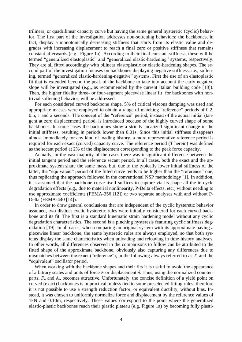
Curiously, all three fits are conservatively biased for almost the entire displacement range

in the case of Figure 16c. They were found to be even more so for extreme steep-mild behav-

ior in Figure 17a. In both these highly curved backbones, a linear softening segment, or a sof-

tening-residual segment combination that would produce near-zero error would need to be

high above and to the right of the actual backbones, clearly enveloping them in the negative

stiffness range. Apparently, the curvature in the shape of the actual backbone has a protective

effect on the system that cannot be replicated by a linear segment and cannot be easily cap-

tured in a practical rule. A possible explanation is that typical ground motion records (e.g.,

non-pulse-like) produce most of the damage in just one or two large pushes within the post-

peak negative stiffness range. Perhaps the change in stiffness, and correspondingly in the tan-

gent period, take the edge off any large nonlinear excursion that can proceed unchecked in a

constant-stiffness linear segment. Especially for the extreme steep-mild case of Figure 17a

this effect is so strong that even using a residual plateau that starts at the intersection of the

two different slopes and maintains the same strength until the ultimate displacement is not

18

enough to reach a fully unbiased solution (Figure 17b). Nevertheless, the latter amendment to

the area-minimization rule was found to be the only simple practical rule that can reliably re-

duce the bias in all such cases to an acceptable level of 20%÷30%. Therefore, this will form

the final part of our “optimal” practical fitting rule.

Figure 16. Generalized elastic-hardening-negative capacity curve having steep-mild (a) and mild-steep (c) nega-

tive slope and the relative median Sa-capacity errors of the secant, Han et al. and balanced fits for T=1.0s.

Figure 17. A generalized elastic-hardening-negative capacity curve having extreme steep-mild negative slope

and its corresponding optimized fit, (a) the curve (b) relative median Sa-capacity errors for T=1.0s.

5 DEFINITION AND TESTING OF THE NEAR-OPTIMAL FIT

Combining all previous results, it is now possible to propose an “optimal” fitting rule that,

while not strictly optimized, manages to maintain low error and low bias and can be standard-

ized to be applicable to a wider range of capacity curve shapes than the ones investigated. Es-

sentially, it is based on fitting the distinct regions of structural behavior that may typically be

observed in realistic pushover curves, namely “elastic”, “hardening” and “softening”; see [25].

19

These will be approximated by linear segments defined by three specific points, namely the

nominal yield (y), the nominal peak strength (p) and the ultimate displacement (u) point:

a) The “elastic” pre-nominal-yield part is captured by a secant linear segment with initial

stiffness matching the secant stiffness of the capacity curve at 5%÷10% of the peak or the

nominal yield base shear. Using the peak is preferable as, without any loss of accuracy, it

allows a fast estimation without needing multiple iterations.

b) The “hardening” pre-nominal-peak non-negative stiffness segment is chosen to terminate

at the maximum base shear while minimizing the absolute area difference (formally the

integral of the difference) of the fitted and the exact curve between the displacements cor-

responding to the nominal peak and the nominal yield points, as defined by the intersec-

tion of this segment with the preceding and succeeding one.

c) The “softening” post-nominal-peak negative stiffness segment is also defined by minimiz-

ing the absolute area difference between the fitted and the exact curve in the negative

stiffness region. It may be further augmented by a fourth, residual plateau segment in two

cases: (i) if the negative stiffness region is characterized by steep slopes that partway

down grow significantly milder, a plateau should be drawn at the intersection of these two

distinct zones; (ii) if instead the negative stiffness progressively grows steeper, then a re-

sidual should be used only if found to improve the fitting according to the area-

minimization rule.

Figure 18. Blind testing sample of (a) capacity curves and (b) their optimized fits.

To properly assess the error induced by the proposed rules, a new sample of curves is

needed. These should not be involved in deriving the rules to achieve objectivity by blind test-

ing. Forty capacity curves were randomly generated, mostly considering relatively highly

curved shapes with non-trivial softening behavior, thus including either steep-mild or mild-

steep negative slopes combined with various rates of change in the initial stiffness, as shown

in Figure 18a. Essentially they are complex shapes created by varying the parameters of the

uniaxial springs composing each SDOF system that are meant to provide a severe test for the

proposed rule. Each curve was fitted according to the “optimal” fitting rule, resulting in the

forty fits showed in Figure 18b. The relative median capacity errors appear in Figure 19 for

0.2s, 0.5s, 1.0s, and 2.0s. To facilitate comparison, the displacement axis has been non-

homogeneously normalized to match the three characteristic points (y, p, u) of the exact push-

over curves. Typical applications of NSP would normally fall within the y and p points. The

mean value of the error never exceeds 20% and the trend is always conservative except for the

first part of the hardening behavior (between y and p points) when low period values are con-

sidered (see Figure 19a). Still, it should be noted that different shape backbones will result to

different errors, in many cases lower than the ones shown due to the deliberate high curvature

of the tested curves.

20

In Figure 20 normal probability plots of the errors are shown at the three characteristic points

for T = 0.2 and 2.0 seconds and for all the forty curves considered, showing a strong resemblance

to a normal distribution. Table 1 shows mean and standard deviation of the relative errors at the

three characteristic points y, p and u, respectively for T = 0.2, 0.5, 1.0, and 2.0s; the data shows

that the distributions are generally conservative (negative errors). Some slightly unconservative

bias can be found only at the yielding point (y) for T = 0.2s. There is also some significant con-

servative bias (red points with negative errors in Figure 20) close at the ultimate point (collapse)

that can be attributed to the abundance of severe steep-mild cases in the tested sample.

Figure 19. The statistics of the relative error in the median Sa-capacity for T = 0.2s, 0.5s, 1.0s, and 2.0s, in the

case of elastic-hardening-negative SDOF systems considered for blind testing of the optimized fit.

Figure 20. Probability plot for normal distribution of the relative errors in the median Sa-capacity evaluated at the

three significant points y, p and u for T = 0.2s and T = 2.0s.

A Kolmogorov-Smirnov hypothesis test [26] was performed on the sample of forty relative

errors at each of the three characteristic points (y, p and u) for each of the four periods. At the

95% significance level this cannot reject the null hypothesis that they follow normal distribu-

tions with the means and standard deviations shown in Table 1; the only exception is the ulti-

21

mate (u) point for T = 0.2s (Figure 20a) due to some large tail values. Using such results, it is

possible to have at least some general sense of the epistemic uncertainty introduced by the

optimized piecewise linear approximation at the three different ranges of behavior. It goes

without saying that the results for current code-based fits are far more dispersed and heavily

biased towards the conservative range.

Table 1. Mean and standard deviation of the relative median error in Sa at the characteristic points y, p, u.

T = 0.2s T = 0.5s T = 1.0s T = 2.0s y p u y p u y p u y p u

0.028 -0.013 -0.086 -0.030 -0.049 -0.143 -0.096 -0.053 -0.163 -0.060 -0.023 -0.122

0.060 0.066 0.182 0.044 0.071 0.218 0.056 0.091 0.186 0.042 0.053 0.129

6 CONCLUSIONS

A near-optimal piecewise linear fit is presented for static pushover capacity curves that can

offer nearly-unbiased low-error approximation of the dynamic response of non-trivial systems

within the framework of Nonlinear Static Procedures. Incremental Dynamic Analysis is used

to rigorously assess different fits on an intensity-measure capacity basis, allowing a straight-

forward performance-based comparison that is largely independent of site hazard. A fitting

rule emerged that is based on using appropriate linear segments to capture the three typical

ranges of structural behavior appearing in realistic pushover curves: (a) “elastic” where the

initial stiffness should always be captured by a secant at 5%÷10% of the peak strength regard-

less of any area-balancing or minimization rules, (b) “hardening”, where it is important to

maintain the actual peak shear strength but not necessarily the corresponding displacement (c)

“softening”, where the ultimate displacement should always be matched while the linear seg-

ment itself should closely fit the negative stiffness pushover curve. In the latter case, if a sig-

nificant lessening of the slope is observed with increasing displacements then an additional

enveloping residual-plateau segment should be employed.

In addition, it was found that simple elastoplastic fits capturing the initial stiffness and the

maximum strength may serve as very simple approximations in most practical situations even

venturing into the early negative stiffness region. On the other hand, all codified approaches

tested generally err on the conservative side, although high changes in initial stiffness may

reverse this finding for certain sites. In general though, the error in code fits always increases

disproportionately when encountering significant changes in stiffness, representative of mod-

els that account for uncracked stiffness or the gradual plasticization and failure of elements. In

particular, the area-balancing fitting process prescribed by most codes is often the culprit. Its

indiscriminate use ignores the strong beneficial effect of backbone shape and curvature, invar-

iably introducing bias. The proposed fit is found to significantly reduce the error introduced

by the piecewise linear approximation, offering a practical solution to upgrade existing guide-

lines.

ACKNOWLEDGEMENTS

The work presented has been developed in cooperation with Rete dei Laboratori Universitari di Ingegneria

Sismica – ReLUIS for the research program funded by the Dipartimento della Protezione Civile (2010-2013).

REFERENCES

1. Fajfar P and Fischinger M. N2 – A method for non-linear seismic analysis of regular

structures. Proceedings of the 9th World Conference on Earthquake Engineering, Tokyo,

Japan; 1988: 111-116.

2. Krawinkler H and Seneviratna GPDK. Pros and cons of a pushover analysis of seismic

performance evaluation. Engineering Structures, 1998; 20: 452-464.

3. Bracci JM, Kunnath SK and Reinhorn AM. Seismic performance and retrofit evaluation of

reinforced concrete structures. Journal of Structural Engineering, 1997; 123: 3-10.

22

4. Elnashai AS. Advanced inelastic static (pushover) analysis for earthquake applications.

Structural Engineering and Mechanics, 2001; 12: 51-69.

5. Antoniou S, Pinho R. Advantage and limitations of adaptive and non-adaptive force-based

pushover procedures. Journal of Earthquake Engineering, 2004; 8: 497-522.

6. Chopra AK and Goel RK. A modal pushover analysis procedure for estimating seismic de-

mands for buildings. Earthquake Engineering and Structural Dynamics, 2002; 31: 561-582.

7. Vidic T, Fajfar P, Fischinger M. Consistent inelastic design spectra: strength and dis-

placement. Earthquake Engineering and Structural Dynamics, 1994; 23: 507-521.

8. Miranda E, and Bertero VV. Evaluation of strength reduction factors for earthquake-

resistant design. Earthquake Spectra, 1994; 10(2): 357-379.

9. National Institute of Standards and Technology (NIST). Applicability of Nonlinear Multi-

ple-Degree-of-Freedom Modeling for Design. Report No. NIST GCR 10-917-9, prepared

by the NEHRP Consultants Joint Venture, Gaithersburg, MD, 2010.

10. Aschheim M, Browning J. Influence of cracking on equivalent SDOF estimates of RC

frame drift. ASCE Journal of Structural Engineering, 2008; 134(3): 511-517.

11. Comitè Europèen de Normalisation. Eurocode 8 – Design of Structures for earthquake resistance

– Part 1: General rules, seismic actions and rules for buildings. EN 1998-1, CEN, Brussels, 2003.

12. Federal Emergency Management Agency (FEMA). Prestandard and commentary for the

seismic rehabilitation of buildings. Report No. FEMA-356, Washington, D.C., 2000.

13. American Society of Civil Engineers (ASCE). Seismic Rehabilitation of Existing Build-

ings, ASCE/SEI 41-06, Reston, Virginia, 2007.

14. Federal Emergency Management Agency (FEMA). Improvement of nonlinear static seis-

mic analysis procedures. Report No. FEMA-440, Washington, D.C., 2005

15. Vamvatsikos D, Cornell CA. Direct estimation of the seismic demand and capacity of os-

cillators with multi-linear static pushovers through Incremental Dynamic Analysis. Earth-

quake Engineering and Structural Dynamics, 2006; 35(9): 1097–1117.

16. Dolsek M, Fajfar P. Inelastic spectra for infilled reinforced concrete frames. Earthquake

Engineering and Structural Dynamics, 2004; 33:1395–1416.

17. Vamvatsikos D, Cornell CA. Incremental Dynamic Analysis. Earthquake Engineering

and Structural Dynamics, 2002; 31: 491-514.

18. CS LL PP Circolare 617. Istruzioni per l’applicazione delle Norme Tecniche per le Co-

struzioni, Gazzetta Ufficiale della Repubblica Italiana 47, 2/2/2009 (in Italian).

19. Ibarra LF, Medina RA, Krawinkler H. Hysteretic models that incorporate strength and stiff-

ness deterioration. Earthquake Engineering and Structural Dynamics, 2005; 34: 1489-1511.

20. Han SW, Moon K, Chopra AK. Application of MPA to estimate probability of collapse of

structures. Earthquake Engineering and Structural Dynamics, 2010; 39: 1259-1278.

21. Vamvatsikos D and Cornell CA. Applied Incremental Dynamic Analysis. Earthquake

Spectra, 2004; 20: 523-553.

22. PEER (2011). PEER NGA Database. Pacific Earthquake Engineering Research Center,

Berkeley, http://peer.berkeley.edu/peer_ground_motion_database.

23. Fragiadakis M, Vamvatsikos D, Papadrakakis M. Evaluation of the influence of vertical

irregularities on the seismic performance of a nine-storey steel frame. Earthquake Engi-

neering and Structural Dynamics, 2006; 35: 1489-1509.

24. Vamvatsikos D. Some thoughts on methods to compare the seismic performance of alter-

nate structural designs. In: Dolsek M. (ed), Protection of Built Environment Against

Earthquakes. Springer: Dordrecht, 2011.

25. Vamvatsikos D, De Luca F. Matlab software for near-optimal piecewise linear approximation

of static pushover capacity curves. [http://users.ntua.gr/divamva/software/bundle_fitSPO.zip].

26. Massey FJ. The Kolmogorov-Smirnov Test for Goodness of Fit. Journal of the American

Statistical Association, 1951; 46: 68-78.