DE-FC26-00BC15311 - National Energy Technology Laboratory

Heavy and Thermal Oil RecoveryProduction Mechanisms

ByAnthony R. Kovscek, Principal Investigator

Louis M. Castanier, Technical Manager

Final Technical Progress Report

For the Period September 1, 2000 – December 31, 2003

Work Performed Under Contract DE-FC26-00BC15311

Prepared forU.S. Department of Energy

Assistant Secretary for Fossil Energy

Sue Mehlhoff, Project ManagerNational Petroleum Technology Office

P.O. Box 3628Tulsa, OK 74101

Prepared byStanford University

Department of Petroleum EngineeringGreen Earth Sciences, Bldg., Room 080B

367 Panama StreetStanford, CA 94305-2220

ii

iii

DISCLAIMERThis report was prepared as an account of work sponsored by an agency of the

United States Government. Neither the United States Government nor any agency

thereof, nor any of their employees, makes any warranty, express or implied, or assumes

any legal liability or responsibility for the accuracy, completeness, or usefulness of any

information, apparatus, product, or process disclosed, or represents that its use would not

infringe privately owned rights. Reference herein to any specific commercial product,

process, or service by trade name, trademark, manufacturer, or otherwise does not

necessarily constitute or imply its endorsement, recommendation, or favoring by the

United States Government or any agency thereof. The views and opinions of authors

expressed herein do not necessarily state or reflect those of the United States Government

or any agency thereof.

iv

ACKNOWLEDGEMENTS

Financial support for research in the area of heavy oil and thermal recoverymechanisms was provided the U.S. Department of Energy under Award No. DE-FC26-00BC15311.

We acknowledge contributions from the Stanford University Petroleum ResearchInstitute (SUPRI-A) Industrial Affiliates. All of these sources of support areacknowledged gratefully.

Aera Energy LLCBP ExplorationChevronTexacoConoco-PhillipsPDVSA IntevepShell Oil Company FoundationTotalTyco Thermal Controls

v

SUMMARY

The Stanford University Petroleum Research Institute (SUPRI-A) studies oilrecovery mechanisms relevant to thermal and heavy-oil production. The scope of work isrelevant across near-, mid-, and long-term time frames. In August of 2000 we receivedfunding from the U. S. DOE under Award No. DE-FC26-00BC15311 that completedDecember 1, 2003. The project was cost shared with industry.

Heavy oil (10 to 20 °API) is an underutilized energy resource of tremendouspotential. Heavy oils are much more viscous than conventional oils. As a result, they aredifficult to produce with conventional recovery methods. Heating reduces oil viscositydramatically. Hence, thermal recovery is especially important because adding heat,usually via steam injection generally improves displacement efficiency. The objectives ofthis work were to improve our understanding of the production mechanisms of heavy oilunder both primary and enhanced modes of operation. The research described spanned aspectrum of topics related to heavy and thermal oil recovery and is categorized into: (i)multiphase flow and rock properties, (ii) hot fluid injection, (iii) improved primaryheavy-oil recovery, (iv) in-situ combustion, and (v) reservoir definition. Technologytransfer efforts and industrial outreach were also important to project effort.

The research tools and techniques used were quite varied. In the area ofexperiments, we developed a novel apparatus that improved imaging with X-raycomputed tomography (CT) and high-pressure micromodels etched with realisticsandstone roughness and pore networks that improved visualization of oil-recoverymechanisms. The CT-compatible apparatus was invaluable for investigating primaryheavy-oil production, multiphase flow in fractured and unfractured media, as well asimbibition. Imbibition and the flow of condensed steam are important parts of the thermalrecovery process. The high-pressure micromodels were used to develop a conceptual andmechanistic picture of primary heavy-oil production by solution gas drive. They allowedfor direct visualization of gas bubble formation, bubble growth, and oil displacement.Companion experiments in representative sands and sandstones were also conducted tounderstand the mechanisms of cold production. The evolution of in-situ gas and oilsaturation was monitored with CT scanning and pressure drop data. These experimentshighlighted the importance of depletion rate, overburden pressure, and oil-phasechemistry on the cold production process. From the information provided by theexperiments, a conceptual and numerical model was formulated and validated for theheavy-oil solution gas drive recovery process.

Also in the area of mechanisms, steamdrive for fractured, low permeabilityporous media was studied. Field tests have shown that heat injected in the form of steamis effective at unlocking oil from such reservoir media. The research reported hereelucidated how the basic mechanisms differ from conventional steamdrive and how thesedifferences are used to an advantage. Using simulations of single and multiple matrixblocks that account for details of heat transfer, capillarity, and fluid exchange betweenmatrix and fracture, the importance of factors such as permeability contrast betweenmatrix and fracture and oil composition were quantified. Experimentally, we examined

vi

the speed and extent to which steam injection alters the permeabillity and wettability oflow permeability, siliceous rocks during thermal recovery. Rock dissolution tends toincrease permeability moderately aiding in heat delivery, whereas downstream thecooled fluid deposits silica reducing permeability. Permeability reduction is notcatastrophic. With respect to wettability, heat shifts rock wettability toward more waterwet conditions. This effect is beneficial for the production of heavy and medium gravityoils as it improves displacement efficiency.

A combination of analytical and numerical studies was used to examine theefficiency of reservoir heating using nonconventional wells such as horizontal andmultilateral wells. These types of wells contact much more reservoir volume thanconventional vertical wells and provide great opportunity for improved distribution ofheat. Through simulation and analytical modeling of the early-time response of areservoir to heating with a horizontal well showed that cyclic steam injection is aneffective technique to heat a reservoir prior to continuous injection during a gravitydrainage process.

New techniques for defining reservoir flow characteristics were developed to helpus improve the recovery efficiency of heavy oil. A streamline approach was proposed anddeveloped for inferring field-scale effective permeability distributions based on dynamicproduction data such as water-cut curve or tracer response. The basic idea is to relateproduction well data directly to the behavior of individual streamlines. Thus, flowpatterns are studied in concert with geology to determine the success of recoveryprocesses. This procedure, is robust, and reduces dramatically the computational size andtime required for history matching and prediction of future recovery history. Extensionsof the procedure show that the method is easily constrained to existing geological data.

INTRODUCTION

The United States continues to rely more extensively on imported oil year byyear. Over the past 25 years, U.S. petroleum consumption has been growing at an averagerate of 0.5% per year. The fraction of oil imported has grown from 28% of U. S.consumption in 1983 to about 55% today. Yet, the current situation has not emergedbecause the U.S. lacks substantial oil and gas resources. Rather, we have not beensuccessful at conducting the research and development to develop cost-effectiveproduction techniques that allow us to convert resources into reserves. A case in point isheavy oil. Estimates place the total heavy resource (less than 20°API) in the WesternHemisphere well in excess of 6 trillion bbl. The heavy oil resource in the U.S. alone is inthe neighborhood of 200 billion bbl. The central problem with heavy-crude-oilproduction is that the oil is far more viscous than water or conventional crude oil.Because fluid flow resistance is proportional to viscosity, high viscosity frustratesproduction.

vii

This project improved our understanding of primary and thermal heavy-oilrecovery mechanisms. As a result, recovery efficiency may increase and oil may berecovered where it is not producible by conventional means. In other words, this projectbegan the development of the pathway to convert heavy-oil resources to reserves.Thermal methods, especially steam injection, where heat is used to lower oil viscosity,and carefully engineered primary (cold) production, are the best techniques for increasingproduction from heavy and fractured reservoirs. Hence, work was focused on thermalrecovery and cold production.

The research tools and techniques employed were varied. Roughly equal weightwas given to experimental investigation as it was to theory development and simulation.A guiding principle for the research effort was that experiments, physical data, andphysical observations provide the ground truth against which models are judged forcompleteness and accuracy. Novel apparatus were developed that allow high-resolutionimaging of multiphase flow through porous media. These apparatus proved invaluable forinvestigating primary heavy-oil production, multiphase flow in fractured and unfracturedmedia, and for probing the effect of temperature on petrophysical properties.

Organization of Report

The research tasks are classified in five broad topical areas: (1) multiphase flowand rock properties, (2) hot-fluid injection, (3) improved primary (cold) recovery, (4) in-situ combustion, and (5) reservoir definition. Technical transfer was integral to theresearch effort. Accordingly, this report is organized to summarize and documentresearch performed in each area as well as to provide a discussion of technical transferefforts and technical achievements.

viii

.

EXPERIMENTAL

Experimental studies were conducted to probe heavy and thermal oil recoverymechanisms. They are discussed in each area, as appropriate. Results obtained andrelated discussion are given in each topic area.

RESULTS AND DISCUSSION

A full spectrum of research in heavy and thermal oil recovery mechansms wasundertaken. Results obtained and related discussion are given in the section, “Resultsand Discussion,” in each topic area.

CONCLUSIONS

Each section lists its conclusions separately.

ix

TABLE OF CONTENTS

Acknowledgements iv

Summary v

Introduction vi

Organization of Report vii

Experimental viii

Results and Discussion viii

Conclusions viii

Area 1. Multiphase Flow and Rock Properties 1References 2

One Dimensional Imbibition, Scaling, and Nonequilibrium Effects 3(Task 1)Introduction 3Experimental One-dimensional Imbibition 3Cocurrent Versus Counter Current Imbibition 5Scaling Group 5Nonequilibrium Effects 9

Mathematical Analysis 10Simulation Results 11Experimental Apparatus 11

Results and Discussion 13Conclusions 13

Dynamic Relative Permeability from CT Data 19(Task 1a)Introduction 19Method 19Results and Discussion 21Conclusions 26References 26

Experimental and Analytical Study of Multidimensional Imbibition inFractured Porous Media 29(Task 1a)Introduction 29Experimental 30

x

Results and Discussion 31Analytical Model 33Physically Correct Transfer Functions 35

Conclusions 41References 42

Foam Generation at Low Surfactant Concentration 43(Task 1b)Introduction 43Model 43Experimental 46Results and Discussion 47Conclusions 52References 53

Scaling of Foamed Gas Mobility in Heterogeneous Porous Media 55(Task 1b)Introduction 55Foam Mobility 56Scaling of Foam Mobility 59Experimental 61Results and Discussion 63Conclusions 70References 71

Thermally Induced Fines Mobilization and Wettibility 75(Task 1c)Introduction 75

Wettability Alteration 75Experimental Investigation 77Surface Forces 82Results and Discussion 85

Quartz-Kaolinite System 86Quartz-Illite System 88


xi

Area 2. Hot-Fluid Injection 94References 95

A Numerical Analysis of the Single-Well Steam-Assisted GravityDrainage Process 96(Task 2a)Introduction 96Model Description 96Results and Discussion 98

Discussion of Early-Time Analysis 100Sensitivity Analysis 100Sensitivity Cases 102Discussion of Sensitivity Analysis 104


Analytical Model for Cyclic Steam Stimulation of a Horizontal Well 106(Task 2a)Introduction 106Model Development 106

Injection and Soak Periods 107Heat Remaining in the Reservoir 109

Production Period 111Property Correlations 113Algorithm for Calculation Scheme 114

Results and Discussion 114Conclusions 119References 120

Efficiency and Oil Recovery Mechanism of Steam Injection Into Low 121Permeability, Hydraulically Fractured Reservoirs(Task 2b)Model Framework 121Results and Discussion 122Efficiency 122Stability in High Porosity Rock 124

Summary 125Conclusions 125References 126

xii

Porosity and Permeability Evolution Accompanying Hot Fluid Injection 128Into Diatomite(Task 2b)References 128

An Experimental Investigation of the Effect of Temperature on Recovery147Of Heavy Oil From Diatomite(Task 2b)Introduction 147Imbibition Potential 148Experimental 149Results and Discussion 150

Outcrop Core/Water/Mineral/Oil 150Outcrop Core/Water/Crude/Oil 151Field Core/Water/Crude/Oil 152Remaining Oil Saturation 153

Interpretation 154Scaling 154Wettability Alteration 155

A Mechanism for Wettability Alteration 158Conclusions 160Nomenclature 161References 162Appendix A-Imbibition Potential 166Appendix B-Experimental Details 169Coreholder 169

CT Scanner 169Rock 170Fluids 170

Procedure 171

Area 3. Mechanisms of Primary Heavy Oil Recovery 173

A Microvisual Study of Solution Gas Drive Mechanisms in Viscous Oils 174(Task 3a)Introduction 174Dynamics of Bubble Growth in Porous Media 175

Diffusion-Dominated Coalescence 176Pressure-Driven coalescence 178

Experimental 183Pressure Vessel 183Optics 186

xiii

Pressure and Fluid Delivery Systems 186Capillary Tube Experiment 187

Results and Discussion 189Viscous Oil 192

Comparison Among Observations and Calculations 196Summary and Conclusions 198Nomenclature 198References 200

Heavy Oil Solution Gas Drive: Effect of Oil Composition and Rock 202Consolidation(Task 2a)References 203

Model and Simulation of Cold Production Using a Population Balance 204Approach(Task 3b)Introduction 204Population Balance Model of Solution Gas Drive 105Results and Discussion 205Conclusion 209References 210

Area 4. In situ Combustion 211Solvent and Air Injection Processes 212(Task 4a)Introduction 212Experimental 212Results and Discussion 213

Metallic Additives 216(Task 4b)Introduction 216Results and Discussion 216

xiv

Area 5. Reservoir Definition 221A Streamline Based Technique for History Matching Production Data 222(Task 5)Introduction 222Precious Work 223Method 224Permeability Updates 227

Steps of the Approach 227Results and Discussion 228Conclusions 234Nomenclature 234References 235

History Matching Constrained to Geostatistical Data 238(Task 5)Introduction 238Gauss-Markov Random Functions (GMrf) 238Integration of GMrf into Streamline-Based History-Matching 239Algorithm 240Results and Discussion – GMrf)

Cases 1: Five-Spot, Isotropic Permeability Field, M=1 241Cases 2: Five-Spot, Isotropic Permeability Field, M=2.5 242Cases 3: Five-Spot, Anisotropic Permeability Fields 249Cases 4: Prediction of Reservoir Performance Using the History-Matched Model M=5 249

Computational Cost 256Remarks 256Streamline-Based Ranking 257

Method 258Conclusions 258References 259

Area 6. Technology Transfer 261Industrial Review Meeting 261Technical Presentations 261

Conference Presentations 262Technical Papers 263

Reviewed Manuscripts 264Website 265Short Course 265International Cooperation 266

IEA Presentations 266

xv

LIST OF TABLES

Area 1. Multiphase Flow and Rock Properties

One Dimensional Imbibition, Scaling, and Nonequilibrium Effects(Task 1a)1. Viscosity of Wetting and Nonwetting Phases 52. Summary of Experimental Systems and the Ratio Viscosities of Wetting and

Nonwetting Phases 6

Dynamic Relative Permeability from CT Data(Task 1a)1. Characteristics of the Berea Sandstone and Diatomite Cores 21

Foam Generation at Low Surfactant Concentration(Task 1b)1. Parameter Values 442. Limiting Capillary Pressure and Surface Tension V (σ from

Bertin et al., 1999) 48

Scaling of Foamed Gas Mobility in Heterogeneous Porous Media(Task 1b)1. Properties of the Porous Media 592. Parameters for Gas-Mobility Calculations 603. Properties of the Porous Media 63

Thermally Induced Fines Mobilization and Wettability(Task 1c)1. Summary of Experimental Conditions 79

Area 2. Hot-Fluid Injection

A Numerical Analysis of the Single-Well Steam-Assisted Gravity Drainage Process(Task 2a)1. Grid, Rock, and Oil Property Description 1012. Operating Conditions for Early-Time Performance Study 102

xvi

Analytical Model for Cyclic Steam Stimulation of a Horizontal Well(Task 2a)1. Physical Properties for Semi-Analytic Calculation and Simulation 115

Efficiency and Oil Recovery Mechanism of Steam Injection Into LowPermeability, Hydraulically Fractured Reservoirs(Task 2b)1. Breakthrough Comparisons in HCPVI for the Three Increasing Porosity

Cases 125

Area 3. Mechanisms of Primary Heavy Oil RecoveryModel and Simulation of Cold Production Using a Population BalanceApproach(Task 3b)1. Porous Medium Characteristics 2052. Fluid Properties 206

Area 4. In-Situ CombustionSolvent and Air Injection Processes(Task 4a)1. Dilution of Cold Lake Crude Oil 2122. Example Calculation for Solvent Injection 2143. Example Production Data 214

Area 5. Reservoir Definition

History Matching Constrained to Geostatistical Data(Task 5)1. Summary of Flow Simulation Parameters for the Four Cases 2422. Computational Work 256

xvii

LIST OF FIGURES


One Dimensional Imbibition, Scaling, and Nonequilibrium Effects(Task 1a)

1. Schematic diagram of imbibition cell (a) exploded view and (b) front viewillustrating injection/production configuration for countercurrent imbibition 4

2. CT-derived saturation maps for counter-current imbibition in water-wetdiatomite. Fluid pairs are indicated on the top of each profile. Time isgiven in minutes beneath each saturation map 6

3. Nonwetting fluid recovery versus absolute time for countercurrent imbibitionwith varying nonwetting fluid viscosity 8

4. Correlation of recovery by countercurrent imbibition from diatomite 9

5. wS versus x plots for different times. Simulations of co-current imbibitionfor a mobility ratio of 0.4 12

6. wS versus tx / plots. Simulations of co-current imbibition(final time: 9.65 h) with four different mobility ratios 12

7. oS versus tx / plots for co-current imbibition in a diatomite core withair/decane system 14

8. wS versus tx / plots for counter-current imbibition in a diatomite core withdecane/water system (total number of pixels: 200) 15

9. oS versus tx / plots for co-current imbibition in a diatomite core withair/decane system (total number of pixels: 300) 15


11. oS versus tx / plots for co-current imbibition in a diatomite core withair/blandol system (total number of pixels: 300) 16

12. wS versus tx / plots for counter-current imbibition in a diatomite core withblandol/water system (total number of pixels: 300) 17

xviii

13. oS versus tx / plots for co-current imbibition in a diatomite core withair/decane system (total number of pixels: 200) 17


Dynamic Relative Permeability from CT Data(Task 1a)

1. Capillary pressure for Berea sandstone 22

2. Experimentally determined water relative permeability curve forBerea sandstone 23

3. Saturation profile obtained by simulation with measured rwk compared tothe experimental profile for Berea sandstone 23

4. Capillary pressure curve used for interpretation of diatomite imbibitionexperiments. Data points are from Akin and Kovscek (1999) 24

5. Experimentally determined water relative permeability curve for outcropdiatomite 25

6. Saturation profile obtained by simulation with measured rwk compared to theexperimental profile for outcrop diatomite 25

Experimental and Analytical Study of Multidimensional Imbibition in FracturedPorous Media(Task 1a)

1. Possible imbibition patterns in (a) 1-D geometry (plane source), (b) 2-D geometry (line source), and (c) 3-D geometry (point source).Lines indicate front position as a function of time 29

2. The core holder: Frontal view 30

3. CT saturation image for 0.32 PV imbibed, “filling-fracture.” Aperture=0.1mm.Injection rate = 1 cc/min. Injection is from lower left corner and productionfrom lower right corner 32

4. CT saturation image for 0.32 PV imbibed. “Instantly-filled fracture.”Aperture = 0.025 mm. Injection rate = 1 cc/min. Injection is from lower leftcorner and production from lower right corner 32

xix

5. The average water saturation in the rock scales linearly with time (“filling-fracture” regime) 33

6. Water Iso-saturation curves for different times obtained with new approach(air-water imbibition, q=1 cc/min, and fw =0.1 mm) 34

7. CT images for “filling-fracture” system for different times. Water injectionat 1 cc/min in a fracture 0.1 mm thick. Injection is from lower left cornerand production from lower right corner 34

8. Schematic representation of the characteristic length versus time 37

9. Shape factor versus time 38

10. Section of the grid (a) and (b) matrix relative permeability and capillarypressure functions used for the numerical simulations 39

11. Comparison of the average water saturation versus dimensionless timeamong the experimental results, analytical model, fine-grid numericalsimulation, and the modified dual-porosity approach 40

12. Comparison of the extent of imbibition between experimental data, analytical model, modified dual-porosity and fine-grid simulation. Fractureaperture = 0.1 mm. Injection rate = 1 cc/min. Injection is from the lower leftcorner 41

Foam Generation at Low Surfactant Concentration(Task 1b)

1. Model transient flowing bubble texture profiles (a) wt% case, (b) 0.1 wt% case; (c) 0.02 wt% case; (d) 0.01 wt% case; (e) 0.005 wt% case 49

2. Experimental (symbols connected by dashed lines) and model (solid lines)transient aqueous-phase saturation profiles. (a) 1 wt% case; (b) 0.1 wt% case;(c) 0.02 wt% case; (d) 0.01 case; (e) 0.005 wt% case 50

3. Experimental (symbols connected by dashed lines) and model (solid lines)transient pressure profiles. (a) 1 wt% case; (b) 0.1 wt% case; (c) 0.02 wt%case; (d) 0.01 wt% case; (e) 0.005 wt% case 52

xx

Scaling of Foamed Gas Mobility in Heterogeneous Porous Media(Task 1b)

1. Prediction of the network model for flowing foam fraction compared to theexperimental data of Friedmann et al. (1991) 57

2. Ratio of gas mobility in low and high permeability zones. Porosity of lowpermeability layer is varied and all other terms held constant 61

3. Apparatus for heterogeneous foam-displacement experiments. The mass flowmeter is removed if foamer solution is injected 62

4. Pressure drop results for gas-only injection into heterogeneous system 64

5. Liquid production from each core for gas only injection into heterogeneoussystem 65

6. Gas Darcy velocity at the inlet to each core and the apparent ratio of sandstoneto A10 gas mobility 66

7. Pressure drop results for simultaneous gas and liquid injection into heterogeneous system 67

8. Liquid production from each core for simultaneous injection of gas and liquidinto heterogeneous system 68

9. Pressure drop response for gas-only and co-injection into A10 syntheticsandstone 69

10. Pressure response for gas-only and co-injection into sandstone 70

Thermally Induced Fines Mobilization and Wettability(Task 1c)

1. Triangles in 1(a) through 3(b) illustrate pore spaces. Gray color symbolizes thewater phase, black color designates oil phase, and round white circlesrepresent clay particles 76

2. SEM images from Berea sandstone core used in experiments. (a) before and,(b) after waterflood 77

3. Experimental apparatus 78

4. Compositional chromatography of effluent fines collected (low salinityinjection, test #2 in core #1, pH=7, 0.01 M NaCl) 80

xxi

5. Permeability change during experiments. Open symbols indicate no fines in effluent, whereas closed symbols indicate fines production 81

6. View of the filtrate collected during test 3 (120°C) from core 2. Brightportions have large density 81

7. Sphere-plate system for modeling fines stability 83

8. Components of sphere-plate interaction and total potential at pH=7 and [Na+]=0.1M 85

9. Experimental and calculated zeta potential as a function of pH at constant salinity (a) Quartz, 1E-3M, NaNO3, (b) Kaolinite, E-4M NaCl 86

10. Detachment temperature obtained for quartz-kaolinite systems with ξ -potential measurements provided by Lorentz. Shading is in degreeCelsius (°C) 87

11. Detachment temperature obtained for quartz-illite system. Shading is in degree Celsius (°C) 89


A Numerical Analysis of the Single-Well Steam-Assisted Gravity Drainage Process(Task 2a)

1. Schematic of grid system: (a) parallel to well bore and (b) perpendicular towellbore 97

2. Recovery factor for the first year of production 98

3. Recovery factor for 10 years of production 99

4. Cumulative steam oil ratio for 10 years of production 99

5. Recovery factor versus time, sensitivity analysis 103

6. Cumulative steam oil ratio, sensitivity analysis 103

xxii

Analytical Model for Cyclic Steam Stimulation of a Horizontal Well(Task 2a)

1. (a) Schematic of heated area geometry; (b) differential element of the heatedarea 107

2. Comparison of semi-analytic model and reservoir simulation results 116

3. Comparison of steam temperature 117

4. Sensitivity of cumulative oil production to the duration of injection 118

5. Sensitivity of cumulative oil production to heat losses 119

Efficiency and Oil Recovery Mechanism of Steam Injection Into LowPermeability, Hydraulically Fractured Reservoirs(Task 2b)

1. Fraction of recovery for multi-layer case 123

2. Cumulative recovery for two different relative permeability curves for the“thief” model. The thermal basecase is compared to the waterflood case 124

Porosity and Permeability Evolution Accompanying Hot Fluid InjectionInto Diatomite(Task 2b)

1. Schematic of experimental setup 129

2. Porosity images for outcrop and field diatomite cores 130

3. Viscosity of oils and brine versus temperature 131

4. Measured interfacial tension between oils and water versus temperature 132

5. Spontaneous water imbibition in oil-field outcrop diatomite core atelevated temperatures: mineral oils 133

6. Spontaneous water imbibition in oil-filled diatomite cores at elevatedtemperatures: crude oil 134

7a Water saturation profile for water imbibition in oil-filled outcrop core(0-10) at 180°C: crude oil 135

xxiii

7b Water saturation distribution at 38.0=Dx versus time for crude oil/outcropcore (0-10) at T = 180°C and wiS 136 136

8a Water saturation profiles for water imbibition in oil-filled field core (F-2) atT=120°C: crude oil 137

8b Water saturation profile for water imbibition in oil-filled field core (F-15) atT=180°C: crude oil 138

8c Water saturation distribution at 35.0=Dx versus time for crude oil/fieldcore (F-15) at T = 180°C and wiS =0 139

9a Water saturation profile for water imbibition in oil-filled field core (F-25) atT=180°C: crude oil (dashed lines indicate forced imbibition) 140

9b Water saturation distribution at 32.0=Dx versus time for crude oil/fieldcore (F-25) at T = 180°C and wiS =30% 141

10. Correlation between remaining oil saturation and temperature for diatomitecore 142

11. Scaled spontaneous water imbibition in oil-filled outcrop diatomite core atelevated temperatures: mineral oils 143

12. Scaled spontaneous water imbibition in oil-filled diatomite cores atelevated temperatures: crude oil 144

13. Effect of temperature on imbibition potential for water imbibition in oil-filleddiatomite core 145

14. Effect of fines production on water imbibition in oil saturated diatomitecore: n-decane 146

Area 3. Mechanisms of Primary Heavy Oil Recovery

A Microvisual Study of Solution Gas Drive Mechanisms in Viscous Oils(Task 3a)

1. Variation in diffusion coefficient of 4CH with oil viscosity 177

2. Variation in gas phase volume with time (constant pressure decline rate) 178

xxiv

3. (a) Side view of two gas bubbles moving towards each other in a narrowpore. (b) Cross-sectional view showing wetting-liquid distribution in a square pore and illustrating the geometry of the corner flow problem 179

4. Example calculation illustrating the effect of oil viscosity on pressure-driven coalescence of two gas bubbles in a cornered capillary 182

5 (a) Pressure-vessel developed for holding micromodels and(b) schematic of apparatus 184, 185

6 (a) Schematic of top view of micromodel illustrating injection andproduction ports and channels and (b) scanning electron microphotographof micromodel etched pore pattern at 500X magnification 187

7. (a) Schematic of capillary tube apparatus for gravity-driven drainage of oillens and (b) optical microphotograph of triangular capillary cross section 188

8. Pressure versus time for pressure depletion of CO 2 saturated water in amicromodel 190

9. Bubble nucleation and growth in CO 2 saturated water: (a) recentlynucleated bubble at 0 s, (b) bubble growth at 0.2 s, (c) gas bubble at 0.9 safter growing to fill pore body, (d) bubbles expand and coalesce at 1.2 s,(e) at 2.4 s bubble expands, (f) bubble is mobilized and leaves the pore spacewhere it was nucleated at 2.8 s 191

10. Repeated bubble nucleation and growth at the same site as shown in Fig. 9a recently nucleated buble at 0 s, (b) bubble growth at 0.5 s, (c) gasBubble at 0.8 s after growing to fill pore body, (d) bubbles expands intoAdjacent pore space at 1.0 192

11. Solubility of CO 2 in the viscous mineral oil Kaydol as a function of pressure 193

12. Pressure versis time for pressure depletion of CO 2 saturated viscous oil in a micromodel 194

13. Bubble nucleation and growth in CO 2 saturated viscous oil: (a) recentlyNucleated bubble at 0 s, (b) bubble growth at 1 min 31 s, (c) gas bubbleGrows to fill pore body at 2 min 50 s, (d) bubbles expands into adjacentPore space at 3 min 6 s, (f) bubble is mobilized and leaves the pore space Where it was nucleated at 3 min 8 s 195

14. Bubble coalescence in viscous oil: (a) three bubbles arrayed in pores at 0 s,(b) coalescence of upper two bubbles at 10 s as gas flows into pore space(c) drainage of thick liquid lens and coalescence of gas bubble at 42 s 195

xxv

15. Distance-time plot of coalescence in capillary tubes. Solid line shows calculations using physical model; dashed lines are experiments 197

Model and Simulation of Cold Production Using a Population BalanceApproach(Task 3b)

1. Match of the IN bubble population balance model to the experimentalpressure data of Firoozabadi et al. (1992). Withdrawal rate is 1.44 cm 3/day(5.10×10-5 ft 3 /day) and the number of bubbles nucleated is 0.0124bubbles/cm 3 (350 bubbles/ft 3 ) 207

2. Match of the IN bubble population balance model to the experimentalpressure data of Firoozabadi et al. (1992). Withdrawal rate is 7.20 cm 3/day(2.50×10 4− ft 3 /day) and the number of bubbles nucleated is 0.0353bubbles/cm 3 (1000 bubbles/ft 3 ) 208

3. Match of the IN bubble population balance model to viscous-oil solutiongas drive pressure data. Withdrawal rate is 6.00 cm 3/hour (2.10×10 4− ft 3 /hr)and the number of bubbles nucleated is 0.490 bubbles/cm 4− ft 3 /day)(14,000 bubbles/ft 4− ft 3 /day) 209

Area 4. In-Situ combustion

Solvent and Air Injection Processes(Task 4a)

1.` Viscosity of mixtures of Cold Lake oil and n-decane. Concentrationreported in volume per cent 213

Metallic Additives(Task 4b)

1. Effluent gas composition, no additives 217

2. Effluent gas composition, tin with 5% Sn cl 2 solution 218

xxvi


A Streamline Based Technique for History Matching Production Data(Task 5)

1. Comparison of permeability fields (a) reference, (b) intial, and (c) historymatched. Shading indicates permeability in md 230

2. Fractional flow curves for test case 231

3. Pressure history for test case 232

History Matching Constrained to Geostatistical Data(Task 5)

1. Reference permeability field, histogram and variogram 100×100 243

2. Permeability field at iterations 1, 2, 5 and 9. The left column is prior tothe GMrf process, while the right is after the GMrf and thereforeconsistent with geology 244

3. History-matched permeability field (100×100), five-spot, M=1 245

4. Match in water-cut, five-spot, 100×100 grid-blocks, M=1 246

5. History-matched permeability field (100×100), five-spot, M=2.5 247

6. Match in water-cut five-spot 100×100 grid-blocks, M=2.5 248

7. Reference permeability field, histogram and variogram 200×200 gridblocks 250

8. History-matched permeability field (200×200 grid-blocks), five-spot, M=1 251

9. Match in water-cut, five-spot, 200×200 gridblocks, M=1 252

10. Reference and history-matched permeability fields 253

11. Match and prediction of water-cut. Matched to a production history of150 days. The rest is prediction 254

12. Match and prediction of cumulative oil production. Matched to a production history of 0.75 PVI. The rest is predictioin 255

1


Application of enhanced oil recovery processes and simulation of these processesdemands understanding of the physics of displacement and accurate representation of constitutiverelations such as relative permeability and capillary pressure. We developed new experimentalapparatus and interpretation procedures to collect this type of information. A common toolthroughout much of the experimental portion of the research is the imaging of oil, water, and gassaturations in situ. This is accomplished primarily through the use of X-ray computedtomography (CT). X-ray CT allows us to obtain the position and shapes of displacement fronts inporous media as a function of time.

Our work in the area of multiphase flow was divided into (a) Imbibition, (b) MobilityControl of Steam, and (c) Temperature Effects of Relative Permeability.

Task 1a considered imbibition in one-dimensional and multi-dimensional systems. Waterimbibition is fundamental to steamdrive and waterflood performance of fractured and unfracturedrocks. The rate and the extent of imbibition depend critically on the wettability of the rock andthe viscosity of the wetting and nonwetting phases. Other factors include: fluid/fluid interfacialtension (IFT), pore structure, the initial water saturation of the rock, and relative permeabilitycurves. Water injection, steam injection, and CO2 injection in a water-alternating gas (WAG)fashion all rely to some extent on capillary imbibition to aid oil production. Steam injection is, forall practical purposes, carried out under saturated conditions with some fraction of the injectedsteam in the liquid phase. Likewise, initial heating of a cold reservoir is accompanied bycondensation and flow of the resulting hot water away from the injector (Hoffman and Kovscek,2003). In CO2 injection under both miscible and immiscible conditions, water slugs are usuallyinjected with the objective of controlling CO2 mobility. Thus, capillary phenomena are importantto most recovery techniques of interest in low permeability media.

Work in Area 1a is summarized in a series of sections. The first section is entitled “Onedimensional imbibition, scaling, and nonequilibrium effects,” whereas the second is “Dynamicrelative permeability from CT data.” The third section that summarizes our efforts in Task 1a is“Experimental and analytical study of multidimensional imbibition in fractured porous media.”

Task 1b examined the gas mobility reduction properties of aqueous foams. Mobilitycontrol of enhanced oil recovery fluids such as steam or CO2 is an important problem. Aqueoussurfactants have shown great promise for gas mobility control. Foam is a dispersion of gas withina surfactant-laden continuous liquid phase. The surfactant provides a measure of stability againstcoalescence of bubbles; foaming surfactants increase significantly the period of time that anyindividual bubble persists. Effective foams can be formed with the addition of surfactantchemical to brine at concentrations on the order of 0.05 to 1 wt%. In the presence of foamed gas,gas and liquid flow behavior is determined by bubble size or foam texture.

Our work in this area was two fold. Effort was directed toward understanding andmodeling foam generation and stability at low surfactant concentrations. Foam displacementexperiments were conducted at a variety of surfactant concentrations in homogeneous one

2

dimensional sandpacks. Modeling and interpretation of the experiments was also accomplished.This work is summarized in the section, “Foam generation and stability at low surfactantconcentration” Second, we expanded our mechanistic model to foam processes in heterogeneousporous media (Kovscek et al., 1997). Specifically, we began with a mechanistic description ofaqueous foam behavior in one-dimensional media and conducted a thorough analysis of how thephysically-based foam-simulation parameters scale with permeability and rock type. The twomajor components of the population balance model considered were bubble size and gasmobility. Bubble size is determined by the interplay of foam generation and coalscence forcesthat are described by rate expressions. Thus, by considering individually the mathematicalexpressions and rate constants describing foam generation and coalescence, we ascertained themanner in which gas-phase mobility shifts as permeability is increased or decreased. This work isentitled “Scaling of foamed gas mobility in heterogeneous porous media.”

Task 1c developed an understanding of the mechanisms by which rocks become morewater wet during thermal operations. Reservoir rocks are thought to become more water wetduring thermal recovery. To date, no plausible mechanism describes this shift toward waterwetness. Fines mobilization presents one pathway to create fresh water wet surfaces. Work inArea 1c is summarized as “Thermally induced fines mobilization and wettability.”

References

Hoffman, B. T. and A. R. Kovscek, 2003. “Light-Oil Steamdrive in Fractured Low PermeabilityReservoirs,” SPE 83491, Proceedings of the SPE Western Region/AAPG Pacific SectionJoint Meeting, Long Beach, CA, May 19-24.

3

One Dimensional Imbibition, Scaling, and Nonequilibrium Effects

(Task 1a)

Introduction

Imbibition studies are naturally divided into experiments that probe behavior in thematrix, flow in fractures, and matrix/fracture interactions. To advance the state of the art ofanalysis of imbibition experiments, we developed an unconventional mode of collecting CT data.In a conventional experiment, X-ray CT data is taken in slices normal to the central (i.e., long)axis of the core or sand pack. The porous medium is translated through the CT scanner in a seriesof steps with a CT exposure collected at every step. Thus, many CT exposures are needed tovisualize the progress of fluid and data is missing from the volume of porous medium lyingbetween scan positions. Figure 1 illustrates the “imbibition cell” that we developed to amelioratethe problems associated with conventional scanning. It is possible to examine the entire length ofa core with a single CT scan. Thus, the cross-section of the coreholder and the water jacket shownschematically in Fig. 1b represents the scanned volume. In addition to providing temperaturecontrol, the shape of the water jacket and the large mass density of water minimizes imagingproblems (cf. Akin and Kovscek, 2003) for a discussion of CT imaging applications and theassociated difficulties). In the schematic, flow is one dimensional and imbibition may occurcocurrently (water and oil flow the same direction) or countercurrently (water and oil flow inopposite directions). The endcaps for the core are designed to accommodate a variety of flowconditions. CT images obtained are of unprecedented resolution and the CT image is easilyconverted to quantitative saturation information.

Experimental One-dimensional Imbibition

The imbibition cell and the unconventional scan geometry became a cornerstone of ourapproach to CT imaging of multiphase flow in porous media. With the apparatus illustrated inFig. 1, we contrasted cocurrent and counter-current flow characteristics, validated a new scalinggroup for one-dimensional counter-current imbibition, demonstrated that it is possible to measureand quantify nonequilibrium multiphase flow effects during cocurrent and counter currentimbibition, and, most importantly, we developed a technique to extract dynamic relativepermeability from the shape and time evolution of saturation profiles measured within theimbibition cell. Each of these advances is discussed briefly.

4

(a)

water in

detector

X-rays

water and produced nonwetting fluid

core

water jacket

endcap

(b)

Figure 1. Schematic diagram of imbibition cell (a) exploded view and (b) front viewillustrating injection/production configuration for countercurrent imbibition.

5

Cocurrent Versus Counter Current Imbibition

There has been considerable debate recently as to whether cocurrent and countercurrentimbibition mechanisms differ fundamentally. The implications are profound for the modeling ofoil recovery from fractured media. The imbibition cell allowed direct measurement of the shapeand time progression of saturation fronts inside of a porous medium imbibing waterspontaneously. Essentially, our experimental results showed that cocurrent imbibition exhibitsdisplacement characteristics that are relatively pistonlike, whereas countercurrent imbibitionprofiles are much more diffuse (Zhou et al., 2002). We interpreted these measurements toindicate that during cocurrent imbibition water advances through pores and throats relativelyuniformly displacing nonwetting fluid. During countercurrent flow, water movement is moredominated by flow along the nooks and crannies of the pore space. Water saturation builds inpore corners whereas the nonwetting fluid occupies the center of pore spaces as well as thelargest pores. Interestingly, an independent study utilizing a new nuclear magnetic resonancetechnique with resolution on the 10 µm scale confirmed and cited our interpretation as acornerstone study (Chen et al., 2003).

Scaling Group

Our interpretation of imbibition displacement also shed new light on scale up ofimbibition phenomena. Scaling of imbibition oil recovery has been pursued for roughly 40 years(Aronofsky et al., 1958; Mattax and Kite, 1962). The chief reason for our dogged pursuit ofscaling is that one extrapolates accurately from the laboratory to the field when scaling isaccurate. Most scaling approaches to date were empirical and did not address the possiblesignificant difference in water and oil mobility that arises for moderately to more viscous oils.Experiments conducted in the imbibition cell illustrated in Fig. 1 employed nonwetting fluidswhose viscosity varied by 4 orders of magnitude (Zhou et al., 2002). Results showedunequivocally that the advance of wetting liquid slows and saturation patterns becomeincreasingly diffuse as the ratio of nonwetting to wetting liquid viscosity increases. Figure 2presents a montage of saturation profiles as measured by X-ray CT for water displacing air, waterdisplacing n-decane (µo = 0.84 cP), and water displacing a viscous mineral oil (µo = 25 cP).Tables 1 and 2 provide a summary of the experimental conditions. The elapsed time from theintroduction of water is given in the figure caption for each exposure for each combination ofwetting and nonwetting fluid. In short, the experimental results taught us that scaling ofcountercurrent imbibition needed to be revisited.

Table 1. Viscosity of Wetting and Nonwetting Phases

Fluid Viscosity (mPa.s)Air 0.018Decane 0.84Blandol 25Water 1.0

6

Table 2. Summary of Experimental Systems and the RatioViscosities of Wetting and Nonwetting Phases

Imbibitionprocess System Ratio of

viscositiesAir - Decane 0.021Co-current Air - Blandol 7.2Decane -Water

0.84Counter-current

Blandol - Water 25

Rather than proceed phenomenologically, scaling of counter current recovery wasexamined theoretically from a fresh perspective. Full details are found in (Zhou et al., 2002).Essentially, flow is assumed to be one-dimensional, gravity is negligible, and the fluid areincompressible. Applying Darcy’s law and invoking capillarity yields after considerablemanipulations:

uw = k1

µwµnw

krnwkrw

M +1

M

∂Pc∂Sw

∂Sw∂x

(1)

where M (= (µnwkrw µw krnw)) is the mobility ratio.

65

0

1Sw

70 77

water-air

water-decane

water-blandol

Figure 2. CT-derived saturation maps for counter-current imbibition in water-wetdiatomite. Fluid pairs are indicated on the top of each profile. Time is given inminutes beneath each saturation map.

7

The form of Eq. 1 results from the restriction to counter-current flow. It suggests thatcounter-current imbibition is diffusion-like and controlled by the product of the mobility in both

phases. Note that the effects of viscosity are accounted for by µnwµw and M +1

M. The

values of the second term are not very sensitive to M, when M is of order unity. However, when

the value of M is substantially different from unity, the contribution of M +1M

can be

significant. The following dimensionless time follows from Eq. 1.

t D = tkφ

σLc

2 λrw

* λrnw

* 1

M* +1

M*

(2)

where λ r* (= kr

* / µ )is a characteristic mobility for the wetting and nonwetting phases and M*

(= λrw* / λ rnw

* ) is a characteristic mobility ratio. Here, end-point relative permeabilities are usedwhen calculating λ r

* and M*. Equation 2 is similar to prior empirically determined (Zhang et al.,1996) scaling of tD with respect to phase viscosity. In the limit of M* approaching unity, tD variesinversely with the geometric mean of µnw and µw. Note also that Eq. 2 explains water/gasimbibition scaling. For water/gas cases, M* <<1/ M* and the scaling of tD with viscosity isapproximately 1/µw as indicated empirically (c.f., Handy, 1960). In short, our work resolves thediscrepancies in scaling of counter current imbibition introduced by prior researchers.

The above discussion is based on the assumption that the relative permeability and thecapillary pressure functions are similar for all of the measurements. In counter-current imbibition,the total water imbibed is controlled by matrix adjacent to the fracture. Thus, if Sw at the inletdoes not vary significantly, the oil recovery is proportional to tD until the imbibition frontreaches the outlet boundary. The capillary driving force, ∂Pc ∂Sw , increases as water saturationdecreases, and, consequently, the imbibition rate is larger at low water saturation than at highwater saturation. Therefore, the oil recovery may depart from tD (see discussion).

To recap, the oil recovery from counter-current imbibition is approximately proportionalto the square-root of time during the initial infinite-acting period. The dimensionless time forcounter-current imbibition can be scaled by Eq. 2, which is more general and explains theempirical findings of Zhang et al. (1996).

Figures 3 and 4 display the efficacy of the scaling group given in Eq. 2. For reference,Fig. 3 presents the raw data as interpreted by CT scanning. Note that recovery rate decreasessubstantially as the viscosity ratio between nonwetting and wetting fluids increases. To obtain oilrecovery, the CT-measured saturation data are averaged over the entire core. Figure 4 summarizesthe new scaling approach. Note that recovery has been scaled to the fraction of recoverable oil.For scaling, the endpoint relative permeabilities must be chosen. In concert with ourinterpretation of relative permeability from spontaneous imbibition dynamics (Schembre andKovscek, 2001, 2003), the end points for water/air displacements are krw

* equal to roughly 0.14

8

and krnw* is chosen as 0.60. In the water/oil cases, krw

* and krnw* are set to 0.14 and 0.45,

respectively. These endpoint values are representative of fine-grained, strongly water-wetdiatomite (Schembre and Kovscek, 2001). The recovery from the water/air system and all of thewater/oil systems agree reasonably well. Within experimental scatter, the data are reduced to asingle curve in spite of the fact that the nonwetting fluid viscosity varies by 4 orders ofmagnitude. The new dimensionless time improves significantly the scaling of spontaneousimbibition in low permeability porous media.

The good scaling of recovery from systems with different viscosity ratios suggests that thegeneral shapes of the recovery curves as a function of dimensionless time are similar over theviscosity range studied. The scaling of the simulation results demonstrate that the end-pointmobility ratio contributes to imbibition rate significantly. The end-point mobility ratio is also ameasure of the wettability of the systems. For strongly water-wet rocks, such as clean sandstone,the relative permeability to water can be very small, resulting in small end-point mobility ratios.On the other hand, for weakly water-wet systems, the water-end point relative permeability canbe large, resulting in large end-point mobility ratios. An interesting application of Eq. 2 asdiscussed later, is that the scaling group is useful for interpreting the wettability of porous media(Tang and Kovscek, 2002A, 2002B).

0

0.2

0.4

0.6

0.8

1

0.0 100 1.0 105 2.0 105 3.0 105

(1) water/air(2) water/n-decane(3) water/blandol(4) water/n-decane(5) water/n-decaneno

nwet

ting

fluid

rec

over

y, fr

actio

n

time (s)

water/air

water/n-decane

water/blandol

Figure 3. Nonwetting fluid recovery versus absolute time for countercurrent imbibitionwith varying nonwetting fluid viscosity.

9

0

0.2

0.4

0.6

0.8

1

0 2 4 6 8 10

water/airwater/n-decanewater/blandolwater/n-decanewater/n-decane

dim

ensi

onle

ss r

ecov

ery,

R

D (=

²Sw

/(1-S

nwr))

dimensionless time, tD

Figure 4. Correlation of recovery by countercurrent imbibition from diatomite.

Nonequilibrium Effects

Imbibition is, fundamentally, a nonequilibrium process (Silin and Patzek, 2003). Byimbibing water, a porous medium is attempting to minimize the free energy of the wetting-nonwetting phase interface and thereby come to a minimum equilibrium state. Nevertheless, ithas been rather difficult to demonstrate conclusively that nonequilibrium effects changesignificantly the flow expected when equilibrium effects dominate flow. The imbibition cellyields experimental results of sufficient precision to allow unambiguous interpretation ofnonequilibrium effects. Our results in this area are unpublished to date. Hence, a fair amount ofdetail is given here to substantiate the approach and results.

This study deals with the processes of counter-current imbibition and the role of non-wetting phase viscosity. We intend to examine imbibition performance over a 5-order ofmagnitude range of non-wetting phase viscosity.

10

Mathematical Analysis

The flow of two immiscible fluids in a porous medium can be modeled using Darcy's andmass conservation laws. In the following mathematical model of counter-current imbibition, localequilibrium is assumed to be reached in both phases. Therefore relative permeabilities andcapillary pressure are unique functions of the water saturation.

Neglecting the gravity forces, Darcy's law in one dimension gives an expression of thevelocity of each phase (Marle, 1981),

uw = −

kkrwµw

∂pw∂x

(3)

and uo = −

kkroµo

∂po∂x

(4)

where k is the permeability, kr the relative permeability, and µ the phase viscosity. The pressurein the two fluids is linked by the capillary pressure:

Pc = po − pw = σ

φk

J (5)

where σ is the interfacial tension, φ the porosity, and J is called the Leverett function. With theassumption of local equilibrium, we can find expressions for J(Sw), krw(Sw) and kro(Sw). Massconservation allows us to link the water saturation to its respective velocity:

φ

∂Sw∂t

+ ∇ .uw = 0 (6)

and

φ

∂(1− Sw )∂t

+ ∇ .uo = 0 (7)

Moreover, if we substitute the expression of uw (Eq. 3) into the Eq. 6, we can write,

∂∂x

( D( Sw ) ∂Sw∂x

) =∂Sw∂t

(8)

with

D( Sw ) = −

kkroφµo

f ( Sw ) dPcdSw

(9)

The function f is called the fractional flow and is defined as

f ( Sw ) =1

1+krokrw

µwµo

(10)

11

Equation 8 is described as a non-linear diffusion equation with a diffusion coefficientequal to D. The diffusion coefficient is a strongly non linear function of saturation and has askewed bell shape (Chen et al., 1995). An important parameter in petroleum engineering is themobility ratio which is defined as:

w

o

ro

rw

kkM

µµ= (11)

Nevertheless, this mathematical model is based on the assumption of local equilibrium.According to Silin and Patzek (2003), the classical equations may not be valid for the first stageof capillary imbibition in a porous medium or at the oil-water interface. Viscous or other modesof dissipation may result in behavior that deviates from the classical formulation.

Simulation Results

The flow simulator Eclipse provides us with saturation values along the core at differenttimes. Some numerical simulations have been performed to model the co-current imbibitionmechanism in an horizontal core so the gravity forces are not taken into account. The code has agrid of 200 blocks and requires the input of rock and fluid properties. The porosity of the rock is0.71, and the permeability is 6.6 mD. The interfacial tension is set to 51.4 mN/m (Zhou et al.,2002). Also, the relative permeability end-points are 1 for oil and 0.5 for water.

Figure 5 shows the plot of the water saturation profiles obtained along the core at differenttimes. Water viscosity is 1cp and oil viscosity is 2.5 cp. Figure 6 displays the plot of the water

saturation versus the similarity variable t

x=η for a variety of mobility ratios.

We note that the saturation profiles collapse for the different times and a given mobilityratio. This is the behavior of a diffusion equation such as Eq. 8. The saturation front appearslarger for a smaller value of the mobility ratio.

Experimental Apparatus

The apparatus shown in Fig. 1 is used to conduct experiments that verify themeasurability of nonequilibrium effects during imbibiton. The setup allows for both co-currentand counter-current imbibition in spontaneous and forced modes. Several experiments have beenconducted in order to analyze the process of counter-current imbibition in diatomite cores. Thevalue of the mobility ratio has been modified by changing the viscosity of the non-wetting phasefrom 0.018 to 0.84 to 25 cp.

0

0.1

0.2

0.3

0.4

0.5

0.6

0.7

0.8

0.9

1

0 0.1 0.2 0.3 0.4 0.5 0.6 0.7 0.8 0.9 1

Normalized x

Sw /

Sw m

ax

t=0.05 hour

t=0.15 hour

t=0.35 hour

t=0.95 hour

t=2.15 hour

t=3.35 hour

t=4.55 hour

t=5.15 hour

t=9.65 hour

Figure 5. Sw versus x plots for different times. Simulations of co-currentimbibition for a mobility ratio of 0.4.

0.00

0.10

0.20

0.30

0.40

0.50

0.60

0.70

0.80

0.90

1.00

0

Sw /

Sw m

ax

Figure 6. S

w

M=6.4 M=0.4

t=1 ht=2 ht=3.2x

.00 0.01 0.02

w versus t

x plots. Simulat

ith four different mobility

M=0.06

12

0.03 0.04 0.05 0.06 0.07

Eta=x/sqrt(t) (m/h^0.5)

ions of co-current imbibition (final time: 9.65 h)

ratios.

13

The core is placed into the special imbibition cell and the waterjacket is filled with waterto limit the artifacts due to the scanning. Liquid can be injected at the top of the core while thebottom face is kept sealed, or vice-versa. For a counter-current imbibition experiment, we injectwater at the top face of the core which has been previously saturated with oil. Due to the capillaryforces, water flows through the pores of the rock and the oil is pushed out. The cylindrical coremade of outcrop diatomite has a length of 9.5 cm and a diameter of 2.5 cm. Samples aremoderately to strongly water-wet. Diatomite is convenient and interesting for study, but resultsobtained are certainly not specific to diatomite.

Results and Discussion

The CT images were analyzed by subtracting images. The porosity and the saturation ofthe wetting phase as a function of time are computed. Figures 7-12 show the standardizedsaturation (ratio of wetting-phase saturation upon maximum wetting-phase saturation) versus the

variable t

x=η for counter-current imbibition processes. The ratio of viscosities wetting

wettingnon

µµ

varies from 0.021 to 7.2 for co-current experiments and from 0.84 to 25 for counter-currentexperiments.

First, none of the data collapses as the classical equations suggest that they should do.This is not simply a case of experimental uncertainty. Data are spread widely, for example Fig.11. Moreover, as time progresses curves progress from the right to the left because η is inverselyproportional to the square root of time.

Second, it seems that curves corresponding to air-oil systems are more spread than thoserepresenting oil-water systems (Figs. 9-14). Lines for different positions x seem to collapse whenviscosities of each phase are closer. This result could be due to nonequilibrium effects which aremore important when viscosities are very different.

Although we obtained the same results in two studies with decane as the non-wettingphase (Figs. 10 and 12), the curves did not collapse for a study with blandol as non-wetting phase(Figs. 14 and 16). It seems that non-equilibrium effects are sensitive to viscosity and the viscosityratio. The pixel number refers to the position into the core where the saturation is computed (pixel0: top of the core and pixel 200: bottom of the core ; total number of pixels: 200).

Conclusions

Based on the local equilibrium assumption, the mathematical study of counter-currentimbibition shows that the equation governing the flow is a type of diffusion equation for bothcounter and cocurrent flow. Therefore, we expect that the plot of water saturation versus thesimilarity variable η collapses all saturation profiles independent of time. Simulations for co-current imbibition exhibit this property of the equations. However, experimental data do not

14

verify this property. Furthermore, it appears that cocurrent and counter-current processes do nothave the same sensitivity to mobility ratio. Also, the shape of some experimental curves could beexplained by nonequilibrium effects. The smaller the mobility ratio, the more important the non-equilibrium effects.

0

0.1

0.2

0.3

0.4

0.5

0.6

0.7

0.8

0.9

1

0 0.001 0.002 0.003 0.004 0.005 0.006 0.007 0.008 0.009 0.01

Eta = x/sqrt(t) (m/s^0.5)

Nor

mal

ized

Sat

urat

ion

So /

So m

ax

pixel 52pixel 62pixel 72pixel 82pixel 92pixel 102pixel 112pixel 122pixel 132pixel 142pixel 152pixel 162pixel 172pixel 182pixel 192pixel 197

Figure 7. So versus t

x plots for co-current imbibition in a diatomite core

with air/decane system.

15

0

0.1

0.2

0.3

0.4

0.5

0.6

0.7

0.8

0.9

1

0 0.001 0.002 0.003 0.004 0.005 0.006 0.007 0.008 0.009 0.01


Nor

mal

ized

Sat

urat

ion

Sw /

Sw m

ax


Figure 8. Sw versus t

x plots for counter-current imbibition in a diatomite core with

decane/water system (total number of pixels: 200).

0

0.1

0.2

0.3

0.4

0.5

0.6

0.7

0.8

0.9

1

0 0.001 0.002 0.003 0.004 0.005 0.006 0.007 0.008 0.009 0.01


Ave

rage

Sat

urat

ion

So /

So m

ax

pixel 82

pixel 92

pixel 102

pixel 112

pixel 122

pixel 132

pixel 142

pixel 152

pixel 162

pixel 172

pixel 182

pixel 192

pixel 202

pixel 212

pixel 222

pixel 232

pixel 242

pixel 252

pixel 262

pixel 272

pixel 282

pixel 290



with air/decane system (total number of pixels: 300).

16

0

0.1

0.2

0.3

0.4

0.5

0.6

0.7

0.8

0.9

1

0 0.001 0.002 0.003 0.004 0.005 0.006 0.007 0.008 0.009 0.01


Ave

rage

Sat

urat

ion

Sw /

Sw m

axpixel 82

pixel 92

pixel 102

pixel 112

pixel 122

pixel 132

pixel 142

pixel 152

pixel 162

pixel 172

pixel 182

pixel 192

pixel 202

pixel 212

pixel 222

pixel 232

pixel 242

pixel 252

pixel 262

pixel 272

pixel 282

pixel 290


x plots for counter-current imbibition in a diatomite

core with decane/water system (total number of pixels: 300).

0

0.1

0.2

0.3

0.4

0.5

0.6

0.7

0.8

0.9

1

0 0.001 0.002 0.003 0.004 0.005 0.006 0.007 0.008 0.009 0.01


Nor

mal

ized

Sat

urat

ion

So /

So m

ax

pixel 72pixel 82pixel 92pixel 102pixel 112pixel 122pixel 132pixel 142pixel 152pixel 162pixel 172pixel 182pixel 192pixel 202pixel 212pixel 222pixel 232pixel 242pixel 252pixel 262pixel 272pixel 282pixel 292pixel 300



with air/blandol system (total number of pixels: 300).

17

0

0.1

0.2

0.3

0.4

0.5

0.6

0.7

0.8

0.9

1

0 0.001 0.002 0.003 0.004 0.005 0.006 0.007 0.008 0.009 0.01


Nor

mal

ized

Sat

urat

ion

Sw /

Sw m

axpixel 52pixel 62pixel 72pixel 82pixel 92pixel 102pixel 112pixel 122pixel 132pixel 142pixel 152pixel 162pixel 172pixel 182pixel 192pixel 202pixel 222pixel 242pixel 262pixel 282pixel 300


x plots for counter-current imbibition in a diatomite

core with blandol/water system (total number of pixels: 300).

0

0.1

0.2

0.3

0.4

0.5

0.6

0.7

0.8

0.9

1

0 0.001 0.002 0.003 0.004 0.005 0.006 0.007 0.008 0.009 0.01


Nor

mal

ized

Sat

urat

ion

So /

So m

ax




with air/decane system (total number of pixels: 200).

18

0

0.1

0.2

0.3

0.4

0.5

0.6

0.7

0.8

0.9

1

0 0.001 0.002 0.003 0.004 0.005 0.006 0.007 0.008 0.009 0.01


Nor

mal

ized

Sat

urat

ion

Sw /

Sw m

ax


Figure 14: Sw versus t

x plots for counter-current imbibition in a diatomite core

with decane/water system (total number of pixels: 200).

19

Dynamic Relative Permeability from CT Data

(Task 1a)

Introduction

The laboratory methods used to calculate relative permeability functions are grouped intocentrifuge, steady- and unsteady-state techniques. The centrifuge method has been improved(Hirasaki et al., 1992, 1995), yet, it has potential pitfalls associated with experiments andinterpretation. Additionally, concerns remain regarding the replacement of viscous forces with arange of centrifugal forces for unsteady state displacement processes that are rate dependent (Ali,1997). Steady- state methods offer disadvantages, especially in the case of low permeability rockswhere it is laborious to reach multiple steady states, and capillary forces and capillary end effectsare significant (Firoozabadi and Aziz, 1988; Kamath et al., 1993). Capillary pressure has asignificant effect on saturation distribution and recovery, and capillary forces dominatemultiphase flow in low-permeability rocks and fractured reservoirs. In developing unsteady-statemethods for low-permeability systems, it is necessary to account for capillary pressure whenobtaining the relative permeability curve. Akin and Kovscek (1999) proved that the use of the(unsteady) JBN technique leads to inaccurate assessment of relative permeability in some cases.Thus, most conventional unsteady techniques do not apply.

Method

In the method proposed here, two-phase relative permeability curves are obtained fromexperimental in-situ, saturation profiles measured during spontaneous imbibition experiments. Apreviously measured capillary pressure versus saturation relationship is needed. Each relativepermeability value at a particular saturation is treated independently when the experiment beginswith low or zero initial water saturation. For experiments where the core is partially saturatedwith water initially, the water saturation increases almost uniformly in time throughout the core.Fitting relative permeability curves to a pre-determined functional shape is not necessary in eithercase. This section proceeds by developing the various equations needed for interpreting the data.In all cases, the relative permeability curve obtained is input for numerical simulation and theagreement between input and computed saturation profiles as a function of time checked.

The equations necessary for data processing of experiments are developed next. Firstcases with little or no initial water saturation are considered. Then, equations appropriate to caseswith medium to high initial water are developed. The method differs slightly between these twocases.

The model begins from one-dimensional flow of two immiscible phases in porous media.The effect of gravity is neglected, but this is not a necessary assumption as shown elsewhere(Schembre and Kovscek, 2003). For the wetting-phase,

uw = −kkrwµw

∂pw∂x

(1)

20

where uw is the Darcy velocity, k is the absolute permeability, krw is the relative permeability, µw

viscosity, and ∂pw∂x

is the pressure gradient of the wetting phase.

The Darcy velocity is a superficial velocity that is identically equal towS

w dtdxSφ .

Substituting this expression for uw in Eq. 1 results in

φSwdxdt Sw

= −kkrwµw

∂pw∂x

(2)

where wSdt

dx is the interstitial velocity of a particular saturation Sw as a function of time and φ is

the porosity. Integrating with respect to time, the relative permeability of a particular Sw is

k rw =x S w Sw

−∂ p w∂ x

S w

dt0

t∫

µ w φk

(3)

In this function, the porosity, viscosity and, permeability are independently measurable andconstant. The position of a particular saturation as a function of time,

wsx and the pressure

gradient history are measured during the experiment. Thus, Eq. 3 allows direct computation of krwsolely from measured data. A similar development for the non-wetting phase yields

krnw =µnwφSnw

k

x Snw∂pnw∂x Snw

dt0t∫

(4)

where ∂pnw∂x

is the non-wetting phase pressure gradient. Equations 3 and 4 are related by the

summation of phase saturations (Sw+Snw) to 1.

In cases with initial water saturation and where the water saturation history is diffuse, it isdifficult to implement the method above. Multiple locations for a given saturation value at aspecific time lead to uncertainty in the assessment of the velocity of the saturation value. Forcases with initial water, a variant of the method of Sahni et al. (1998) for gravity drainage isdeveloped.

The Darcy velocity and conservation equation for each phase are again used. Rather thanintegrating Darcy’s Law, the material balance for each phase is integrated. The in-situ saturationmeasurement and an independently measured capillary pressure relationship are still needed. The

21

result for the wetting phase is,

krw = −µwφ

k

∂Sw∂t x, t

dx∫

∂pw∂x x ,t

(5)

and similarly, for the non-wetting phase,

krnw = −µnwφ

k

∂Snw∂t x ,t

dx∫

∂pnw∂x x, t

(6)


An extensive validation exercise for this approach is documented elsewhere (Schembreand Kovscek, 2003). Here, we focus on a demonstration using experimental data obtained fromthe imbibition cell. Water saturation profiles measured by X-ray CT during spontaneousimbibition water imbibition into air-filled Berea sandstone and diatomite are used. The propertiesof each system are summarized in Table 1. The column "voxel resolution" refers to the number ofCT-measured saturation data along the z-axis of the core.

Table 1: Characteristics of the Berea Sandstone and Diatomite Cores

Berea sandstone DiatomitePorosity[fraction] 0.22 0.68Permeability[md] 780.0 6.6Diameter[cm] 2.43 2.43Length [cm] 8.8 9.02voxel resolution* 210 225

*total number of measured Sw values along z-axis of core

The imbibition capillary pressure curve given by Sinnokrot et al. (1969) for Bereasandstone, was modified for different fluid system and petrophysical properties (ie, k, φ) by usingthe Leverett J-function (Leverett, 1941; Ma et al., 1991) That is, the required curve was first non-dimensionalized and then rescaled according to k,φ, and σ (θ=0). The capillary pressurerelationship used in this case is shown in Fig. 1. The relative permeability curve obtained isshown in Fig. 2. The values of krw obtained are reasonable. Moreover, the endpoint krw obtainedagrees with endpoints found in the literature for Berea sandstone (Lerdahl et al., 2000; Oak et al.,1990).

A comparison of the CT-determined experimental water saturation profiles versus timeand the profiles obtained by simulating the core with the measured relative permeability is shownin Fig. 3. The results match especially well given the scatter in the experimental data. Notice thatthe shape and position of the imbibition front are well reproduced. Since the pressure gradientwithin the core was not measured in the experiments, it was not possible to find the non-wetting

22

phase relative permeability. A linear krg relationship is used for simulation. Because the gas isinviscid, the shape of krg versus Sw has little effect on the computed saturation profiles in Fig. 3.

We also used diatomite during experiments because there is very little known aboutpetrophysical properties in diatomite. The use of the classical unsteady state method in thedetermination of relative permeability for diatomite surely leads to inaccurate results because oflow permeability and corresponding capillary effects. The same experimental method as in thecase of the Berea sandstone was used to obtain the water saturation profiles. The core is initiallyair-filled.

0

10000

20000

30000

40000

50000

60000

0 0.1 0.2 0.3 0.4 0.5 0.6 0.7 0.8

Sw

Pc(p

a)

Figure 1. Capillary pressure for Berea Sandstone.

23

0.000001

0.00001

0.0001

0.001

0.01

0.1

10 0.1 0.2 0.3 0.4 0.5 0.6 0.7 0.8

Sw

Krw

Figure 2. Experimentally determined water relative permeability curve for Berea sandstone.

0

0.1

0.2

0.3

0.4

0.5

0.6

0.7

0.8

0 0.01 0.02 0.03 0.04 0.05 0.06 0.07 0.08 0.09

X[cm]

Sw

0.033333333

0.108333333

0.166666667

0.233333333

hr

hr

hr

hr

Figure 3. Saturation profile obtained by simulation with measured krw compared tothe experimental profile for Berea sandstone.

24

The input imbibition capillary pressure curve was measured with the porous-plate methodas reported by Akin and Kovscek (1999). It is similar to another curve reported by Kumar andBeatty (1995), but not shown here. The capillary pressure used is given in Fig. 4. The relativepermeability curve obtained from the measured Sw profile is shown in Fig. 5. At high watersaturation, the relative permeability is found to decrease as Sw increases. The reason for thisartifact is shown in Fig. 6. Here, the experimental water saturation profile and the profile obtainedby simulating the imbibition process are compared. High water saturations within the experimentsadvance slowly at earlier time. Note the first profile for a time of 0.0069 hr. This is indicative offlow that is not one dimensional at small times. Therefore, retardation exists for saturation valuesgreater than 0.7. The solid line gives the relative permeability curve used for simulation:

krw(Sw ) = 5E−5 exp(8.3355 Sw ) (7)

Despite the difficulties in measuring krw at large Sw, the results obtained from simulation(solid line) with Eq. 7 match the saturation-history data well, as shown in Fig. 6. Additionally, thedata points in Fig. 6 and the extrapolation at high water saturations indicate a low endpoint valueof roughly 0.2 for krw. This is indicative of and consistent with the strong water-wetness of thesecore samples (Akin et al., 2000; Zhou et al., 2002).

0.0E+00

2.0E+05

4.0E+05

6.0E+05

8.0E+05

1.0E+06

1.2E+06

1.4E+06

1.6E+06

1.8E+06

0 0.1 0.2 0.3 0.4 0.5 0.6 0.7 0.8 0.9 1Sw

Pc

[pa]

Capillary Pressure used in method

Capillary pressure reported inSPE54590

Figure 4. Capillary pressure curve used for interpretation of diatomite imbibitionexperiments. Data points are from Akin and Kovscek (1999).

25

0.0001

0.001

0.01

0.1

1

0 0.1 0.2 0.3 0.4 0.5 0.6 0.7 0.8 0.9

Sw

Krw

Figure 5. Experimentally determined water relative permeability curve for outcrop diatomite.

0

0.1

0.2

0.3

0.4

0.5

0.6

0.7

0.8

0.9

1

0 0.01 0.02 0.03 0.04 0.05 0.06 0.07 0.08 0.09 0.1

X[cm]

Sw

0.006944444

0.4125

0.6625

0.995833333

1.679166667

Figure 6. Saturation profile obtained by simulation with measured krw compared to theexperimental profile for outcrop diatomite.

26

Conclusions

In summary, a method has been developed to determine dynamic relative permeabilityfrom the water saturation profile history obtained during X-ray CT monitored spontaneousimbibition experiments. The method was tested using synthetic data for the water-air and water-oil cases. In addition, the method was adapted for cases with large initial water saturation.Computed relative permeability values matched well the input curves, suggesting reliability forthese systems. In the water-oil case, discrepancies among the measured and input oil relativepermeability values were attributed to numerical inaccuracies in the simulator. The air-phasepressure gradient can be neglected in the calculations of water relative permeability. A sensitivitystudy showed that neglecting the oil-phase pressure gradient might lead to error in high watersaturation values for viscous oils.

The procedure was used to determine the water relative permeability for two experimentalcases with Berea sandstone and quarried diatomite. In both cases, the relative permeability curvesobtained were used to simulate the experimentally measured water saturation profile versus time.The computed saturation history reproduced the experimental behavior well. Importantly, thismethod allows measurement of relative permeability from a single experiment. Potentially thisrepresents a great time savings.

References

Akin, S., Kovscek, A.R., 1999. Imbibition studies of low-permeability porous media, SPE 54590.Proceedings of the SPE Western Regional Meeting, Anchorage, May 26-29.

Akin, S. and Kovscek, A.R. 2003. “Computerised Tomography in Petroleum EngineeringResearch,” in Applications of Computerized X-ray Tomography in Geology and RelatedDomains, Jacobs, P., Mees, F., Swennen, R, Van Geet, M. (eds), Special Publication,Geological Society, London.

Chen, Q, Gingras, M. K., and Balcom, B. J., 2003.“ A Magnetic Resonance Study of Pore FillingProcesses During Spontaneous Imbibition in Berea Sandstone,” Journal of ChemicalPhysics, 119(18) 9609-9616.

Chen J., et al. 1995. “Theoretical investigation of counter-current imbibition in fractured reservoirmatrix blocks”, SPE 29141, Feb.

Firoozabadi, A., Aziz, K., 1988. Relative permeabilities from centrifuge data, SPE15059.Proceedings of the 56th California Regional Meeting of the SPE, Oakland, April 2-4.

Handy L., Determination of effective capillary pressures for porous media from imbibition data,Petroleum Transactions, AIME, 1960.

27

Hirasaki, G.J., Rohan, J.H., Dudley, J.W., 1992. Modification of centrifuge and software fordetermination of relative permeability curves, SPE 25290. Proceedings of the AnnualTechnical Conference, Washington D.C., October 4-7.

Hirasaki, G.J., Rohan, J.H., Dudley J.W., 1995. Interpretation of oil-water relative permeabilitiesfrom centrifuge experiments, SPE 24879. SPE Adv. Tech. Series. 3 (1). 66-75.

Kamath, J., deZabala, E.F., Boyer, R.E., 1993. Water/oil relative permeability endpoints ofintermediate-wet, low permeability rocks, SPE 26092. Proceedings of the WesternRegional Meeting, Anchorage, May 26-28.

Kumar, M., Beatty, F.D., 1995. Cyclic steaming in heavy oil diatomites, SPE 29623. Proceedingsof the Western Regional Meeting, Bakersfield, March 8-10.

Lerdahl, T.R., Øren, P., Bakke, S., 2000. A predictive network model for three-phase flow inporous media, SPE 59311. Proceedings of the SPE/DOE Improved Oil RecoverySymposium, Tulsa, April 3-5.

Leverett, M.C., 1941. Capillary behavior in porous solids. Petroleum Transactions, AIME 142,152.

Ma S., Jiang, M. X., Morrow N.R., 1991. Correlation of capillary pressure relationships andcalculations of permeability, SPE 22685. Proceedings of the 66th Annual TechnicalConference and Exhibition, Dallas, October 6-9.

Marle C.M., Multiphase flow in porous media, Editions Technip, 1981.

Mattax, C. C. and Kyte, J. R. (Jun 1962). “Imbibition Oil Recovery from Fractured Water-DriveReservoirs.” Soc. Pet. Eng. J. 2: 177-184.

Oak, M.J., Baker, L.E., Thomas, D.C., 1990. Three-phase relative permeability of Bereasandstone. Journal of Petroleum Technology 42. 1054-61, August.

Sahni, A., Burger, J., Blunt, M., 1998. Measurements of three phase relative permeability duringgravity drainage using CT scanning, SPE 39655. Proceedings of the SPE/DOE ImprovedOil Recovery Symposium held at Tulsa, April 19-22.

Schembre, J. M. and A. R. Kovscek, 2001. " Direct Measurement of Dynamic RelativePermeability from CT-Monitored Spontaneous Imbibition Experiments," SPE 71484Proceedings of the SPE Annual Technical Conference and Exhibition, New Orleans, Sept.30 - Oct. 3.

Schembre, J. M. and A. R. Kovscek, 2003. "A Technique for Measuring Two-Phase RelativePermeability in Porous Media via X-ray CT Measurements, Journal of Petroleum Scienceand Engineering, 39(1&2), 159-174.

28

Silin, D. and T. W. Patzek, 2003. “On Barenblatt’s Model of Spontaneous CountercurrentImbibition,” Transport in Porous Media, to appear.

Sinnokrot, A.A., Ramey, H.J., Marsden, S.S., 1969. Effect of temperature level upon capillarypressure curves, SPE 2517. Proceedings of the SPE 44th Annual Fall meeting, Denver,Sept 28-Oct. 1.

Tang, G.Q. and A. R. Kovscek, 2002 "Experimental Study of Heavy Oil Production fromDiatomite Core at Elevated Temperatures, " SPE 75132 Proceedings of the SPE/DOEThirteenth Symposium on Improved Oil Recovery, Tulsa, April 13-17.

Tang, G-Q. and A. R. Kovscek, 2002B. "Wettability Alteration of Diatomite Induced by Hot-Fluid Injection" SPE 77461, Proceedings of the SPE Annual Technical Conference andExhibition, San Antonio, Sept. 29 - Oct. 2.

Zhang, X., Morrow, N. R. and Ma, S. 1996. “Experimental Verification of a Modified ScalingGroup for Spontaneous Imbibition.” Soc. Pet. Eng. Res. Eng. 11: 280-28.

Zhou, D., L. Jia, J. Kamath, and A. R. Kovscek, 2002. “Scaling of Counter-Current ImbibitionProcesses in Low-Permeability Porous Media,” Journal of Petroleum Science andEngineering, 33(1-3), 61-74.

29

Experimental and Analytical Study of Multidimensional ImbibitionIn Fractured Porous Media

(Task 1a)

Introduction

Our understanding of imbibition behavior in fractured systems, and models for matrix-fracture transfer, are largely based on such one-dimensional experiments as reported above.Nevertheless, even a rudimentary exploration of imbibition suggests than mechanisms in morethan one dimensions are intricate. For example, the transfer of water and oil across the matrixfracture interface is governed by a balance of viscous forces driving flow through fracture andcapillary suction that draws water out of the fracture. Similarly, imbibition time scales can besignificantly large and comparable to the time required to fill fractures with wetting fluid. Thus,the overall time scaling for imbibition may differ from the results given in one-dimensionalexperiments.

Figure 1 illustrates schematically how time scaling differs with dimension. Where initialwater saturation is low, results (e.g., Akin et al., 2000) have shown in one-dimensional media thatthere is a well-defined spreading front parallel to the surface exposed to the imbibing fluid. Thisfluid advances at a speed proportional to the square root of time, as shown in Fig. 1a. This is thebasis for the so-called "square root of time models" of imbibition. Assume that the same physicalprocess occurs in all directions in multidimensional porous media, even against the force ofgravity. Next, consider a two-dimensional medium where water imbibes from a stationary linesource, Fig. 1b; the progress of water imbibition in the x-direction is proportional to the squareroot of time, and, likewise, in the z-direction. Thus, in two-dimensional media, the overall massof water imbibed is proportional to the product of the extent of imbibition in each direction.Imbibition in this case should scale linearly with time. Later, this is shown to be trueexperimentally. Finally, this analysis suggests that three-dimensional water imbibition from apoint source scales with time to the three-halves power, Fig. 1c.

Figure 1. Possible imbibition patterns in (a) 1-D geometry (plane source),(b) 2-Dgeometry (line source), and (c) 3-D geometry (point source). Linesindicate front position as a function of time.

30

Experimental

Experimental equipment was designed based upon our success with the unconventionalscan geometry of the one-dimensional imbibition cell. The apparatus insures minimal artifactswhile imaging and the collection of maximum saturation information. It is described next.

Due to the cubic geometry of the cores as illustrated in Fig. 2 and our desire to measurein-situ saturations with X-ray CT, conventional core holders could not be used. The basic idea ofthe experimental design given in Fig. 2 is to avoid drastic changes of the density of the objectscanned by presenting a circular cross-section to the scanner. Initially the outside surface of theBerea sandstone (Cleveland Quarries) samples were coated and sealed with Marine Epoxy (TapMarine Plastic #314). The cores were then potted in vertical cylindrical PVC containers with thesame epoxy. Once the core was covered by epoxy in the PVC container, the bottom face of thecylinders was cut open to expose the rock. Sufficient core was removed so that no trace of epoxyremained on this face (verified by subsequent CT scans).

Rock Sample

Water jacket

PVC container

Fracture

End-cap

Injection Distribution Port

ProductionDistribution Port

Acrylic Secondary Container

Figure 2. The core holder: Frontal view

This PVC core-holder was placed in a second horizontal cylindrical acrylic container, asshown in Fig. 2. A cylindrical shape was used to allow the core to be rotated in any positionaround the horizontal axis. Once filled with water, the second container serves as a water jacketto lessen the contrast in density between the acrylic and PVC/epoxy and to achieve some measureof temperature control. Thus, the cross-sectional shape for scanning is symmetric and circular,improving image quality. The scanning plane is the cross section shown in Fig. 2.

31

Acrylic end-caps were machined to mate with the circular PVC core-holder. The end capshave 2 perforations (inlet and outlet) to give planar 2D flow across the face of the block. The end-caps (one at the top and one at the bottom) were attached to the PVC coreholder by means ofthrough bolts and sealing O-rings. Fracture apertures were set by means of metallic shims(essentially feeler gauges of precise thickness) placed between the block and end-cap. Thus, auniform fracture aperture is guaranteed along the entire core. Using this system, fluids areinjected and produced in any combination desired. The end-caps are also shaped so that core andend-caps fit the inner diameter of the water jacket when assembled. This combination of end-caps, core, and water jacket allowed the coreholder to be set in a unique position. Identical crosssections are compared from experiment to experiment.

Prior to each experiment, cores were dried to zero water saturation in a vacuum oven. Thecore holder was assembled and the fracture aperture set. A number of experiments at constantwater injection rates into the fracture were conducted. Injection rates varied from 0.1 cc/min to 4cc/min. Different fracture apertures also were used, going from very narrow (0.025mm) to wide(0.1 mm). Setting the flow rate with fixed fracture thickness, CT images were obtained to observethe progress of multidimensional imbibition. Water was injected on the left and produced fromthe right-hand side in order to have uniform advance of water along the bottom face of the core.Once the injection started, the core was scanned at the same location for successive times. Furtherexperimental details and the equations for processing of the raw CT images are given by Rangel-German and Kovscek (2002).


Figures 3 and 4 show typical experimental results and illustrate the presence of twodifferent fracture-flow regimes. Both images were taken after 0.32 PV of water had imbibed intothe core. White shading indicates water and black shading indicates air. Both systems have aninjection rate into the fracture of 1cc/min. The chief difference between the two experiments isthe fracture aperture. A wide fracture of 0.1 mm (Fig. 3) leads to relatively slow water advancethrough the fracture and a two-dimensional imbibition pattern. On the other hand, the fracturefills with water quickly when the aperture is narrow, 0.025 mm (shown in Fig. 4, the imbibitionpattern is one-dimensional in this case). We have coined the behavior illustrated in Fig. 3 as the“filling-fracture” regime whereas that shown in Fig. 4 is termed an “instantly-filled” fracture.

The instantly-filled behavior is analogous to one-dimensional imbibition and requireslittle further comment here. The filling-fracture regime shows a variable length plane source dueto relatively slow water flow through fractures. Water horizontal advance is controlled by theinteraction between the matrix and the fracture as shown in Figs. 3 and 4. Because the advance ofwater in the horizontal and vertical directions each scale linearly with the square root of time, themass of water imbibed scales linearly with time. That is, the mass imbibed in this two-dimensional geometry is proportional to the product of these two length scales.

32

wS

Figure 3. CT saturation image for 0.32 PV imbibed, “filling-fracture."Aperture = 0.1 mm. Injection rate = 1 cc/min. Injection is fromlower left corner and production from lower right corner.

wS

Figure 4. CT saturation image for 0.32 PV imbibed. “Instantly-filled fracture”.Aperture = 0.025 mm. Injection rate = 1 cc/min. Injection is fromlower left corner and production from lower right corner.

Figure 5 summarizes the "filling-fracture" portion of all air-water experiments conducted.Within experimental uncertainty, the mass imbibed scales linearly with time before the advancingwater front reaches the end of the fracture. Note that Fig. 5 shows an experiment where the initialwater saturation was about 0.22. The rate of imbibition is less because capillary forces are weakerthan the cases with zero initial water saturation; however, a linear relationship between the massof water imbibed and time is apparent.

33

0

0.1

0.2

0.3

0.4

0.5

0.6

0 100 200 300 400 500 600

time [sec]

Ave

rage

Wat

er S

atur

atio

n

wf=0.025mm,q=0.5cc/min








Figure 5. The average water saturation in the rock scales linearly with time("filling-fracture" regime).

Analytical Model

The experimental results indicate clearly the existence of at least two regimes duringcapillary-dominated imbibition in fractured porous media. A precursor to developing morephysical expressions for matrix-fracture transfer to be employed in numerical reservoirsimulators is to develop an analytical model that describes the experiments. The model is usefulfor scaleup, for describing matrix-fracture transfer in a multiblock system, and if integratedprovides the functional dependence with time of shape factors that describe matrix-fracturetransfer in simulation.

Full details of the model are given by Rangel-German and Kovscek (2002, 2003). Insummary, the imbibition process is approximated by a diffusion-like equation with a capillary-pressure-based hydraulic diffusivity. Three assumptions were used: 1) the water saturation in thematrix is constant initially, 2) the water saturation in the matrix at an infinite distance from thefracture remains constant, and 3) the convection/diffusion equation with constant diffusivity, αh,applies for this problem. Linear superpostion is used to develop the saturation distribution ofwater in the matrix. Mass balance is applied to track the progress of water in the fracture.

Figure 6 displays typical results from the analytical model. Compare to Fig. 7 and it isfound that the model well represents the experiment. The characteristic time, tc, is the boundarybetween imbibition regimes. It can be found implicitly from Eq. 20 when X is set to the fracture

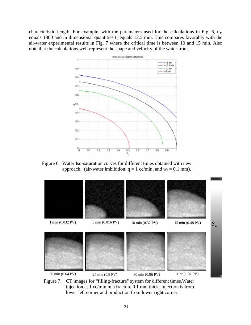
34

characteristic length. For example, with the parameters used for the calculations in Fig. 6, tDcequals 1800 and in dimensional quantities tc equals 12.5 min. This compares favorably with theair-water experimental results in Fig. 7 where the critical time is between 10 and 15 min. Alsonote that the calculations well represent the shape and velocity of the water front.

Figure 6. Water Iso-saturation curves for different times obtained with newapproach. (air-water imbibition, q = 1 cc/min, and wf = 0.1 mm).

5 min (0.016 PV) 15 min (0.48 PV)1 min (0.032 PV)

20 min (0.64 PV)

10 min (0.32 PV)

30 min (0.96 PV)25 min (0.8 PV) 1 hr (1.92 PV)

wS

Figure 7. CT images for “filling-fracture" system for different times.Waterinjection at 1 cc/min in a fracture 0.1 mm thick. Injection is fromlower left corner and production from lower right corner.

35

The model allows us to develop explicit expressions for the rate of water transfer to thematrix, Rff,. In the filling fracture regime the rate is obtained as

Rff =dQm (t)

dt= qw,inj 1− etD erfc tD[ ]( ) (1)

where the dimensionless time is

t D = 4φ

φf

2α hw f

2 t (2).

In these equations, Qm is the volume of water imbibed into the matrix, qw,inj is thevolumetric injection rate of water into the fracture, φ is the matrix porosity, φf is the fractureporosity, αh= kkrw/µw (dPc/dSw) is the hydraulic diffusivity of the matrix, and wf is the fractureaperture. The rate of transfer in the instantly-filled regime, Rif, is a constant with respect to thesquare-root of time. Thus for both regimes and accounting for initial water saturation, Swi, theequation for average water saturation in the matrix block is:

Sw = t Rff 1− H(t − tc )[ ]+ tc Rff + (t −tc)0.5 Rif[ ]H(t −tc )+ Swi (3)

where H is the Heaviside function; and tc is the characteristic time for the fracture. Thecharacteristic time, tc, is the boundary between both regimes. The fracture fills instantly withrespect to the matrix if tD (= t/tc) is large.

Physically Correct Transfer Functions

Our next goal was to reduce the experimental data and the analytical model to a formappropriate for inclusion in a dual-porosity reservoir simulator. Due to the variable-extent of theimbibing area in the filling-fracture regime, it cannot be approached in as straight-forward afashion as the instantly-filled fracture regime. To obtain a characteristic, dimensionless solution, adimensional analysis is performed. It has two objectives: (i) to obtain a better understanding ofthe definition of shape factor within the dual-porosity/dual-permeability formulation, and (ii)provide a general shape factor for any kind of geometry, shape and regime that can be applied tocurrent commercial numerical simulators without major coding complications.

One of the general dual-porosity (and dual-permeability) or MINC models is that theseformulations were developed for pseudo-steady state flow between the fracture and the matrix,and/or uniformly distributed fractures that are totally immersed instantaneously. As shown bothexperimentally and analytically in the previous sections (and detailed in Rangel-German, 2002),there is a sizeable and varied suite of physical phenomena such as fractures being partiallycovered by water or parallel fractures that are not necessarily connected, and therefore thepressure distribution between them is non-uniform. These cases lead to more efficient ultimaterecovery because they occur as co-current flow modes. Current numerical formulations lack the

36

ability of matching the transient behavior in the matrix or considering blocks that are partiallycovered by water and, therefore, lead to overly pessimistic predictions of performance.

Discrepancies exist for values of shape factors proposed by different investigators.Exponential approximations or using only the first term of the summations in the analyticalsolutions helps keep the calculations efficient by giving a constant shape factor; however, theseapproaches do not necessarily capture the physics of the process. Apparently, this is a commoncase of trade-off between computational efficiency and accuracy. Nevertheless, the definition ofthe transfer function

τ =σ k V

µpm − pf( ) (4)

suggests a physically accurate formulation that is also computationally efficient. Equation 4 is aDarcy's law type equation applied to a characteristic distance from the fracture to some positionwithin the matrix block. Dimensional analysis teaches that σ is expressed as:

σ(t) =A(t)

V l* (t) (5)

where A(t) is the area of the matrix block contacted by water, V is the bulk volume of the rockmatrix block and l* is the distance between the saturation at the fracture and the matrix averagesaturation, wS . Thus, the transfer function due to imbibition is

( )wmwhSw SSV −= maxαστ (6)

with σ calculated using Eq. 5.

The analytical model summarized in the previous section also includes an equation for thewater advance in a single fracture in the presence of capillary imbibition into adjacent matrixblocks. This equation was obtained by coupling the matrix and fracture implicitly, and it is usedhere to derive or estimate the transfer functions needed in numerical reservoir simulation. Thearea of the matrix block contacted by water, A(t), is obtained easily as shown by Rangel-Germanand Kovscek (2002).

The only term missing to compute the shape factor in Eq. 5 is the distance between thewater saturation at the fracture and the matrix average water saturation, l*. For a steady-stateproblem, it is clear that l* is the half distance between the fractures (i.e. half-length of the matrixblock). However, for unsteady state behavior such as early-time filled-fracture or during thefilling-fracture regime, the behavior of l* is not obvious. In this work, a simple analytical methodto obtain l* is proposed. The integral of the saturation distribution over the entire domain (n-D, ifneeded) is equal to the average saturation in the matrix times a characteristic distance to thecentroid of the domain. The characteristic distance, l*, for one set of fractures is

37

l*(t ) =Sw(x,t)0

Lx∫ dxSwm (t)

(7)

thus, l* depends on the shape of the matrix block. Figure 8 shows a schematic of the distance, l*

for water saturation, as a function of time.

l*(ti)

t

l*

Figure 8. Schematic representation of the characteristic length versus time.

An analogous σ(t) is needed when dealing with pressure; thus, l*p is obtained in a manner

similar to Eq. 7, but using the pressure solution and the average pressure in the matrix:

lp* (t) =

pw (x,t)0Lx∫ dx

pwm (t) (8)

The characteristic length, l*, is computable from experimental results obtained with CT scanning.Every CT image (corresponding to a single time) of every experiment is translated into a bitmapfile containing the water saturation value at each pixel. The integral of Eq. 7 is calculatednumerically. Then, one computes the average water saturation in the matrix. Figure 9 illustrates aplot of the shape factor, σ(t), calculated by means of Eqs. 6 and 8 against dimensionless time,

2x

hD L

tt α= , on a log-log plot. Four different experiments from Rangel-German and Kovscek (2002)

that span a variety of behavior are analyzed. These integrals (Eqs. 7 and 8) can also be obtainedfrom the analytical or numerical solution of the distribution of saturations and pressures,respectively.

38

Figure 9. Shape factor versus time.

All of the experiments converge to the constant shape factor, σ*, at the same characteristicdimensionless time of approximately, t*

D = 0.1. In general, the new shape factor is written as:

σ = σ*tDtD*

−m

for tD < tD* (9)

andσ = σ* for tD ≥ tD

* (10)

where t*D is 0.1 and m is a function of the flow rate and the fracture aperture. Note that this

formulation converges to the classical constant σ, and also has a time varying portion for tD lessthan tD

*. This makes its implementation in any dual-porosity simulator relatively straightforward.Alternately, the time dependence could be converted to an aqueous phase saturation dependencethat is a function of matrix-block geometry, capillary pressure, and relative permeabilityfunctions.

Figure 9 also provides information on the physics of the fracture filling and imbibitionprocesses. For instance, the experiment performed at a flow rate and fracture aperture of 2.0cc/min and 0.025 mm, respectively, corresponds to a narrow fracture filling rapidly at a high flowrate; therefore, the one-dimensional advance occurs early in the experiment and the centroid ofthe average water saturation, l*, is closer to 0.5 as the front becomes more uniform. This case

39

exhibits the smallest and most constant σ during the transient period. On the other hand, theexperiment performed at a flow rate and fracture aperture of 0.5 cc/min and 0.1 mm, respectively,corresponds to a relatively wide fracture filling slowly at a low flow rate (see Fig. 3). Thecentroid of the average water saturation has a small value initially; hence a large value of shapefactor is obtained. It is important to mention that both the instantly-filled and filling-fractureregimes display similar behavior when using the definition of shape factor given by Eq. 5. Thus,the expression for shape factor is general.

A numerical validation of the proposed shape factor is presented next with comparisonsmade to the experimental data, analytical model (above), the modified dual-porosity formulationwith the new time-dependent shape factor and transfer function, and full-physics numericalsimulation. The new dual-porosity formulation was coded into a simple simulator. Additionally, afine-grid numerical simulation was also performed to match the results using Eclipse 100(Geoquest 2000). Figure 10(a) illustrates a section of the grid used in the numerical simulation.The matrix block is described by a 10x10x10 grid, and the fracture is comprised in a 10x10x1grid with dimensions corresponding to the experimental apparatus shown in Fig. 2. Fig. 10(b)illustrates the matrix capillary pressure and relative permeability functions. The fine-gridsimulation aims to mimic both the CT-experimental and analytical results; therefore, properties ofboth matrix and fracture are the same as those from the experiments described in Rangel-German(2003). Full details of the set up of the validation are given in Rangel-German and Kovscek(2003).

(a) (b)

Figure 10. Section of the grid (a) and (b) matrix relative permeability and capillarypressure functions used for the numerical simulations.

Figures 11 and 12 contrast the results with all of the approaches. Figure 11 shows theaverage water imbibed versus time. Agreement among all approaches is excellent; but of coursethe analytical and new dual-porosity approaches execute much more quickly than the fine-gridsimulation. Figure 12 compares the extent of imbibition (iso-saturation curves/maps) for different

40

times obtained with the experimental set-up, the analytical model described in the previoussections, the modified 'dual-porosity' approach, and the fine-grid simulation. The squares withinthe modified dual porosity portion of Fig. 12 illustrate the fraction of the matrix filled with water.Figure 12 indicates that not only does the analytical model and now dual-porosity approach getthe imbibed volumetrics correct, but the water is also distributed correctly.

Figure 11. Comparison of the average water saturation versus dimensionless timeamong the experimental results, analytical model, fine-grid numericalsimulation, and the modified dual-porosity approach.

41

Figure 12. Comparison of the extent of imbibition between experimental data, analyticalmodel, modified dual-porosity and fine-grid simulation. Fracture aperture =0.1mm. Injection rate = 1 cc/min. Injection is from the lower left corner.

Conclusions

In summary, the pseudo-steady state approach for describing matrix-fracture transfer leadsto constant shape factors. However, multi-phase flow in fractured porous media is not well-approximated by this assumption as illustrated by our experiments. Clearly, there are multiplemodes of fracture and matrix fill up. The behavior of the shape factor is clearly time dependent,and therefore the use of a constant shape factor is incorrect. Formulations for modeling flow infractured porous media were, thus, reconsidered. One of the advantages of the new shape factor isthat it is based on dimensional analysis. It embodies the full physics of matrix-fracture transfer.

42

References

Akin, S., Schembre, J.M., Bhat, S.K., and Kovscek, A.R., 2000. Spontaneous imbibitioncharacteristics of diatomite. J. Petrol. Sci. & Eng., 25: 149-165.

GEOQUEST, 2000. Eclipse 100 Technical Description 2000A, GeoQuest, Schlumberger.

Rangel-German, E. R. and A. R. Kovscek, 2002. "Experimental and Analytical Study ofMultidimensional Imbibition in Fractured Porous Media," Journal of Petroleum Scienceand Engineering, 36(1-2), 45-60.

Rangel-German. E. R. and A. R. Kovscek, 2003. “Time-Dependent Matrix-Fracture ShapeFactors for Partially and Completely Immersed Fractures,” SPE 84411, Proceedings of theSPE Annual Technical Conference and Exhibition, Denver, Oct. 5-8.

43

Foam Generation at Low Surfactant Concentration

(Task 1b)

Introduction

This project was designed to obtain an understanding of how overall recovery, pressuredrop profiles, and water saturation profiles shift with changing surfactant concentration. There areboth theoretical and experimental components. A quantitative model is necessary to interpret theexperimental results to follow, because the mechanisms of gas mobility reduction by foam derivefrom the flow resistance of discrete bubbles. Thus, it seems natural to compute directly gasmobility from the texture or number concentration of bubbles inside porous media. A balance thattracks the evolution of the number concentration of bubbles is one means to link bubbles and gasmobility. Foam is treated mathematically as a nonreactive, time-dependent component of the gasphase. Previous work has formulated a population balance approach that is mechanistic in thatwell documented foam mechanisms are incorporated into a continuum balance equation for foam(Kovscek et al., 1995; Kovscek et al., 1997). The theory reproduces well experimental foambehavior at surfactant concentrations around 1 wt%. However, this approach has not been testedover a variety of surfactant concentrations and especially at low concentration where foam isweak.

Model

In addition to the requisite material balances for water, surfactant, and nitrogen chemicalspecies, a transient balance on the mean bubble size is written. In one dimension (Kovscek et al.1995):

∂∂t

φ S fn f + Stnt( )[ ]+∂∂x

uf nf( )= φSg k1vwv f1 /3 − k−1v f n f[ ]+ Qb (1)

where t denotes time, φ is porosity, S is saturation, n is bubble concentration (bubbles per unitvolume of gas), u is Darcy velocity, v is the interstitial velocity (v = u / Sφ), k1 is the generationrate constant, k-1 is the coalescence rate constant, and Qb is a source/sink term for bubbles. Thesubscript f refers to flowing foam, t to trapped foam, g to the gas phase, and w to the aqueousphase. Units of the various terms are listed in Table 1. We refer to number concentration, foamtexture, and bubble texture synonymously throughout this work.

Note the similarity of Eq. 1 with the usual mass and energy balances for transportprocesses in porous media. The first term on the left of Eq. 1 is the accumulation of foam bubblesand the second term is the flux of foam bubbles. The first term on the right of Eq. 1 represents thenet generation of foam bubbles, i.e., generation minus coalescence. Foam generation is taken as apower-law expression that is proportional to the interstitial liquid velocity multiplied by the 1/3power of the gas velocity. The origin of these velocity dependencies for generation may be foundelsewhere (Kovscek and Radke, 1996).

44

Table 1. Parameter Values

Two-phase flowparameters

Population balanceparameters

parameter value parameter valuek 7 µm2 k1 7.5 x 1012 s1/2m-13/3

φ 0.35 ko-1 100 m-1

a 3 α 2.5 x 10-14

Pas2/3m10/3

b 1.8 Xf 0.10ko

rw 0.7ko

rg 1 Capillary pressureafter Pruess

function(1987)

Swir 0.06µw 1.0 mPa-sµg 0.018 mPa-s

Pc = σφk

1.417(1 − Swd)(−2.120(1 − Swd )2 +1.263(1 − Swd )3)

Foam coalesces when bubbles flow into so-called termination sites (Jiménez and Radke,1989; Kovscek and Radke, 1994). Hence, foam coalescence is taken as proportional to theinterstitial flux of foam, vfnf. The coalescence rate constant varies strongly with the localcapillary pressure, surfactant formulation, and aqueous-phase concentration. A high rate ofcoalescence is expected at low surfactant concentration because there is little surfactant to exert astabilizing effect. A dramatically lower rate is expected when the concentration is high and thesurfactant is known to produce stable foam, provided that the porous medium does not exceedlimiting capillary pressure.

The effects of surfactant concentration and capillary pressure are embodied in thecoalescence rate constant. The following functional relationship is employed:

k−1 = k−1o Pc

Pc* − Pc

2

(2)

where k-1o is a scaling factor that is set constant and Pc

* is the limiting capillary pressure, k-1becomes very large as Pc and Pc

* approach equality. Khatib et al. (1988) first suggested thatfoam-film strength was directly related to gas mobility reduction in the presence of foam. For agiven surfactant and concentration, they observed dramatic foam coarsening at a particularcapillary pressure that they termed the "limiting capillary pressure,” Pc

*. Above Pc*, foam films

are unstable, coalescence of foam lamellae is significant, and high gas mobility emerges. BelowPc

*, coalescence is significantly less and gas mobility is low. The major task of this work is toinfer the functional form of Pc

* with respect to surfactant concentration from laboratoryexperiments and to simulate these experiments quantitatively.

45

To solve Eq. 1, additional information on the convection of foam and wetting aqueousphase is required. Darcy’s law is retained including the formalism of multiphase relativepermeability curves. For the gas phase, we replace viscosity with an effective viscosity relationfor foam:

µ f = µg +αnf

v f1/ 3 (3)

where α is a constant of proportionality. This expression follows directly from theoretical studiesof bubble flow in capillary tubes and porous media (Bretherton, 1961; Hirasaki and Lawson,1985; Wong et al. 1995a, 1995b).

Foam also reduces gas mobility by reducing the gas-phase relative permeability. Becausethe portion of gas that actually flows partitions into the largest pores with the least flowresistance, we employ a so-called “Stone-type” relative permeability model (Stone, 1970),although the ideas employed here predate Stone (Saraf and Fatt, 1967). Hence, the relativepermeability of the flowing foam is only a function of Sf. Because the wetting phase partitionsselectively to the smallest pore space, the aqueous-phase relative permeability is unaffected byflowing and stationary foam. This statement is well established by experiment (Bernard et al.,1965; Holm, 1968; Sanchez et al., 1986; Huh and Handy, 1989; DeVries and Wit, 1990).Aqueous phase relative permeability remains solely a function of Sw. Clearly, the relativepermeability of the stationary foam is zero. A standard exponent relative permeability model is

used

krw = krwo Swd

a (4a)

krf = krgo S fd

b (4b)

with a and b representing the exponents for water and gas flow, respectively. The superscript oindicates the endpoint relative permeability. The reduced saturations, Sid, are written

S fd = X f (1 − Swd ) (5a)

Swd =Sw − Swir( )1− Swir( ) (5b)

where Xf = Sf/Sg is the fraction of the gas phase that is flowing and Swir is the irreducibleaqueous-phase saturation. The relative permeability exponents and endpoint relativepermeabilities represent values for non-dispersed, continuum gas-liquid flow in the porousmedium.

46

Experimental

The apparatus consists of a 0.51 m (20 in) long aluminum sandpack with a 0.051 m (2 in)inner diameter. It was packed with dry 100-120 mesh Ottawa sand in an upright position andpneumatic vibrators were used to ensure good settling. Screens at the inlet and outlet faces of thesandpack prevented washout of sand grains. The average porosity and permeability of pack 1 are35% and 6.7 µm2, whereas for pack 2 the values are 36% and 7.0 µm2. CT images, as describedlater, confirmed that the packs were homogeneous. Permeability values reported are permeabilityto brine.

The sandpack attaches to an L-shaped mounting bracket for bolting of the apparatus to aprecision positioning system (Compumotor, RP240, Parker Hannifin Corp.). Displacements wereconducted with the core oriented horizontally. Positioning errors are not detectable with thissystem. Note that the geometry for CT scanning is conventional so that multiple cross sectionsare examined as the core translates through the CT scanner. The core length is too great to besuitable for the unconventional geometry employed in our imbibition studies. Fairly long porousmedia need to be used during foam experiments because the inlet sections of cores are subjectedto strong foam generation and coalescence forces embodied in Eq. 1.

Aluminum pressure taps were welded to the surface of the coreholder. Each tap wasmachined to accept a filter and thereby sand migration through the tap was avoided. Pressureresponse was measured by a single Paroscientific pressure transducer (model 43K-101) connectedto a 7-way valve. Measurement of six independent pressures is possible. The valve was switchedmanually and a PC was used to collect absolute pressure data from the transducer. The totalacquisition time for a set of pressure data is roughly 30 to 40s.

Nitrogen and surfactant solution are co-injected at constant rates using a Matheson 0-10SCCM (standard cubic centimeters per minute) mass flow meter (model 8240) and an ISCO(model 500D) syringe pump, respectively. Experiments are conducted at backpressures ofroughly 690 kPa (100 psi) using a Grove Mitey-Mite dome loaded backpressure regulator (ModelS-91LW).

In-situ saturation information was collected with the CT scanner. Scans were made on 13cylindrical volume sections perpendicular to the central axis of the core. Scan locations were notevenly spaced so that scanning through pressure ports was avoided. The acquisition time of oneimage is 7 s and the processing time is about 40 s. The total time of measurement is short enoughto capture accurately the position of the front. Raw CT number data are converted to porosityand saturation distribution information according to the algorithms summarized by Akin andKovscek (2003).

The surfactant used to make the foamer solution is an α-alpha olefin sulfonate (AOS1416) supplied by Shell Chemical Co. Sodium chloride (NaCl) at a concentration of 0.5 wt% indistilled water was the brine. Surfactant solution concentrations employed in the experimentswere 0.005, 0.01, 0.02, 0.1, and 1.0 wt% active surfactant. The less concentrated solutions wereprepared by diluting the 1 wt% foamer solution with a 0.5 wt% brine. The critical micelleconcentration (CMC) of the solution is roughly 0.005 wt% (Bertin et al. 1999) and the nominalsolution viscosity is 1 mPa s.

47

The experimental procedure is relatively simple. The pack was prepared and mounted onthe positioning system and then N2 was injected to assure a dry pack. The system back pressurewas increased to 690 kPa (100 psi) and dry CT scans were made at the prescribed positions.Carbon dioxide (CO2) was injected to displace the N2. At least 10 pore volumes of 0.005 wt%foamer solution were injected to saturate the pore space with liquid and satisfy adsorption ofsurfactant to the sand. The advantage of CO2 is that it dissolves readily in water ensuring that allgas is removed. Periodically, the pressure lines were opened to purge any gas that hadaccumulated. Then wet CT images were collected.

The gas-liquid mixture was not foamed before injection and the injection rates areconstant throughout the experiments. The foamer solution injection rate was fixed at 0.07 mL/minand the gas flow was set to 3.8 SCCM (standard cubic centimeters per minute). This translates toa superficial gas velocity of about 0.39 m/d and a gas fractional flow of 88% at the nominalsystem back pressure of 690 kPa. The total superficial velocity, including liquid injection, is 0.44m/day.

Following the completion of an experiment, the core was flushed with CO2 and thencopious (10-20 PV) amounts of foamer solution of the next larger concentration were injected toresaturate the sandpack. The CT scanner was used to monitor the progress of resaturation therebyverifying that all gas had been ejected from the core. The experiments were performed in order ofincreasing surfactant concentration to assure that surfactant desorption from solid did not affectresults. The first pack (6.7 µm2) was used for solutions of 0.005, 0.01, 0.02, and 1 wt% surfactant,and the second pack (7 µm2) was employed for the 0.1 wt% solution.


To model the transient foam displacements, Eqs. 1-4 are solved with a standard fully-implicit, simultaneous-solution finite difference method with upstream weighting of the phasemobilities. Additionally, water and nitrogen mass balances are computed. Because the sand packsare presaturated with surfactant solution, there is no need to compute a surfactant mass balance.The primary variables are water-phase pressure, gas-phase saturation, and bubble density.Boundary and initial conditions mirror the experiments: gas and liquid are injected at constantmass rates and the outlet pressure is fixed at 690 kPa (100 psi). The surfactant and gas are notfoamed before injection. Therefore, no bubbles are injected and Qb is set to zero. The initialconditions include Sw equal to 1, nf equal to 0, and the appropriate uniform surfactantconcentration depending upon the experiment under consideration.

Tables 1 and 2 list the model parameters including standard multiphase flow informationas well as population balance parameters. Also given in Table 1 is the capillary pressure versuswater saturation function (Pruess 1987). The parameter α in the expression for effective foamviscosity varies with surface tension (Hirasaki and Lawson 1985). As Table 2 shows, the surfacetension changes by only 2.9 mN/m over the entire range of concentrations employed.Accordingly, α is held fixed in the simulations to follow. The ratio of foam generation tocoalescence rate constants, k1/ko

-1, was chosen to yield bubbles with undistorted spherical radii ofabout 0.4 mm for the 1 wt% case. Further information on parameter estimation for population

48

balance models is discussed in some detail elsewhere (Kovscek and Radke 1994; Kovscek et al.1995).

Table 2. Limiting Capillary Pressure and Surface TensionV(σ from Bertin et al., 1999)

Concentration (wt%) σ (mN/m) Pc* (kPa)

1.0 31.1 30.40.10 31.9 17.60.020 32.8 7.190.010 33.1 3.670.005 34.0 2.34

The critical capillary pressure, Pc*, as a function of surfactant concentration is required to

simulate the experiments. Because the surfactant concentration in each experiment is constant, weset Pc

* at each concentration rather than assuming a functional form for Pc* versus surfactant

concentration. Table 2 lists the value of Pc* found for each concentration and the experimentally

determined surface tension as a function of concentration for this particular surfactant at a brineconcentration of 0.5 wt%. As expected, Pc

* is large when the surfactant concentration is largeand decreases as the concentration approaches the CMC (Aronson et al., 1994).

The modeling results for foam texture evolution at each surfactant concentration arepresented first. Unfortunately, no experimental method exists to measure directly foam texture insitu. High surfactant concentration results are shown first and then subsequent simulations atlower concentration follow. Next, the effect of foam texture on gas mobility is judged frommeasured and computed aqueous-phase saturation profiles as a function of time. Pressure dropprofiles and the match between experiment and model complete this section.

The predicted bubble concentration along the length of the core as a function of time isgiven for each of the different surfactant concentrations in Fig. 1. Figure 1a represents the largestconcentration while Fig. 1e shows the lowest. Time is given nondimensionally in pore volumes oftotal injection with the exit pressure used to calculate the volumetric gas rate. In Fig 1a,representing the 1 wt% concentration experiment, a region of net generation is found near theinlet. Bubble concentration is nearly constant at all time levels beyond roughly the first quarter ofthe sand pack until the concentration peaks immediately upstream of the front. Physically, the netrate of foam generation is large at the front. Thus, the bubble concentration goes through amaximum before decreasing to zero downstream of the front where there is no gas, and hence, nobubbles (Kovscek et al., 1997). The relatively constant foam concentration between the inletregion and the foam front is about 22 bubbles/ mm3. A foam bubble of this size has a diameter ofroughly 0.44 mm when taken out of the porous medium and allowed to assume a spherical shape.For the simulation of the 1 wt% concentration, the breakthrough time of bubbles is about 1.2 PVI.

The bubble concentration profiles shown in Fig. 1b for the 0.1 wt% concentration arelower than the values for the 1 wt% case. The lower surfactant concentration results in a lessercritical capillary pressure for foam coalescence, as given in Table 2. As a result, the foamcoalescence rate increases and the average bubble concentration decreases. Disregarding the inlet

49

region and the elevation of bubble concentration at the front, the flowing bubble concentration inthis case is about 3.5 bubbles/ mm3 corresponding to an undistorted spherical bubble diameter of0.82 mm.

Figure 1. Model transient flowing bubble texture profiles (a) 1 wt% case; (b) 0.1 wt% case;(c) 0.02 wt% case; (d) 0.01 wt% case; (e) 0.005 wt% case.

An elevation in foam texture in the region of the front is also found in the lower surfactantconcentration cases. The process of snap-off of gas bubbles is purely a mechanical process andcontinues regardless of the concentration of surfactant. This is reflected in the net foamgeneration rate of Eq. 1. As a consequence, bubbles are always generated when the watersaturation is high and the capillary pressure is less than critical such as when gas first enters awater saturated region of the porous medium. Foam coalescence forces quickly destroy most ofthis initial foam because the surfactant concentration is low and thus the limiting capillarypressure for foam coalescence is reached quickly. Correspondingly, the magnitude of the

50

elevation in foam texture at the front also decreases with decreasing surfactant concentration. InFig. 1c the maximum texture is 8 bubbles/ mm3 while in Fig. 1d it is 4 bubbles/ mm3. There islittle difference in the bubble texture profiles of Figs. 1d and 1e because the limiting capillarypressure, as given in Table 2, has changed little between these two cases.

Figure 2. Experimental (symbols connected by dashed lines) and model (solid lines)transient aqueous-phase saturation profiles. (a) 1 wt% case; (b) 0.1 wt% case;(c) 0.02 wt% case; (d) 0.01 wt% case; (e) 0.005 wt% case.

The one-dimensional aqueous-phase saturation profiles as a function of time for each caseare presented in Fig. 2. Time is again given nondimensionally in pore volumes. One dimensionalsaturation data is obtained by averaging the voxel by voxel CT-measured saturations for eachcross section. In Fig. 2, symbols give the experimentally measured points and they are connectedby dashed lines to guide the eye. The solid lines represent model predictions based upon the foamtextures in Fig. 1 and Eqs. 3 to 5 for gas mobility. In general, transient displacement is efficientwhere bubble concentrations are large such as in the 1 wt% surfactant concentration case in Fig.

51

28a, and displacement efficiency decreases as surfactant concentration and bubble texturedecrease. Also note that the saturation change across the front is steep and sharp when the foam isstrong as shown in Figs 2a and 2b.

The match between experiment and model is quite good in all cases prior to breakthroughand the onset of end effects, except perhaps the 0.005 wt% case. Displacement efficiency declineswith decreasing surfactant solution concentration in both the simulations and experiments. Also,notice that the predicted saturation profiles across the displacement front in Figs. 2c through 2ebecome more diffuse as the surfactant concentration decreases. Predictions echo experiments inthis regard. It is important to recall that these results are not achieved by history matching eachexperiment. The only parameter that changes in each simulation is the value of Pc

*. Thisparameter is physical and directly related to surfactant concentration (Aronson et al., 1994).

The experimental displacement results summarized in Fig. 2e show a region at x/Lroughly equal to 0.35 where desaturation of the aqueous phase is inefficient. Displacement is notuniform across the cross section, and a region of 100 % aqueous phase saturation remains in theupper portion of the cross section. The simulations are one dimensional and cannot account forsuch selective displacement at low surfactant concentration. Nevertheless, the simulationsreproduce, qualitatively, the low displacement efficiency at this surfactant concentration.

The second type of in-situ data collected was pressure drop. The lower limit of accuracyfor the pressure measurement system used is about 0.14 to 0.34 kPa (0.02 to 0.05 psi).Experimental and simulated pressure drop profiles as a function of time are presented in Fig. 3 foreach of the surfactant concentrations. The match between model and experiment is acceptable.Large bubble concentrations lead to significant gas-phase flow resistance and low aqueous-phasesaturation. Therefore, the 1 wt% case with the finest bubble texture, as shown in Fig. 3a,demonstrates the largest overall pressure drop. As the bubble textures decline with surfactantconcentration, the predicted pressure drops decline also.

For the 1 wt% and 0.1 wt% cases in Figs. 3a and 3b where significant foam and pressuredrops are generated, it is easy to distinguish the foam-filled region of the sand pack in thepressure drop profiles. For example in Fig. 3b at 0.41 PVI, a relatively steep pressure gradientdue to the presence of foam extends from the inlet to x/L equal to 0.43. The pressure drop in theremainder of the sand pack is small corresponding to the single-phase flow of water.

To improve the clarity of Figs. 3c to 3e, a legend displays the symbol and timecorresponding to each experimental data point. Difficulties were encountered in measuring thesmall pressure drops characteristic of the lower surfactant concentrations, especially at the inlet ofthe sandpack. Gas migrated into some of the pressure lines during the experiment. In theseinstances, large, aphysical, positive pressure gradients were measured. These erroneous pressuredata likely originated from gas entering the sintered filters inside the pressure taps. Accordingly,erroneous pressure information has been deleted from Figs. 3d and 3e. The portion of the datapresented in Fig. 3c that is in error is not clear, so all information is retained. Despite theseproblems, experiment and simulation agree on the general magnitude of pressure drop.

A feature of the model that bears further discussion is the predicted pressure drop profilesfor the low surfactant concentration cases in the region immediately upstream of the foam front.

52

Examine the pressure profile at 0.44 PVI in Fig. 3c and the corresponding bubble concentrationprofile in Fig. 3c. The pressure gradient is relatively shallow in the foam-filled region exceptimmediately before the front. Here, the gradient is much steeper than in the front region becausebubble concentration is elevated at the front. This elevation in texture reduces gas mobilitycausing the pressure gradient to steepen.

Figure 3. Experimental (symbols connected by dashed lines) and model (solid lines)transient pressure profiles. (a) 1 wt% case; (b) 0.1 wt% case; (c) 0.02 wt%case; (d) 0.01 wt% case; (e) 0.005 wt% case.

53

Conclusions

An experimental study of foam generation and propagation as a function of aqueoussurfactant concentration was conducted in 7 µm2, homogeneous sand packs. The in-situ phasesaturation and pressure distribution were measured during the experiments. As expected, thedisplacement efficiency decreases and gas mobility increases with decreasing surfactantconcentration. This experimental trend indicates that foam weakens as the surfactantconcentration decreases. However, even weak foam improves displacement somewhat.

Such results are best understood considering the role of foam bubble size, orsynonymously foam texture, in setting the mobility of foamed gas in porous media. Many smallbubbles result in a low mobility foam and few large bubbles result in a high mobility foam. Foambubbles, at fixed injection rates of liquid and gas, grow in volume as surfactant concentrationdecreases because foam coalescence forces are inversely proportional to surfactant concentration.

These ideas are expressed quantitatively by the incorporation of the role of foam textureon displacement in porous media using a mechanistic, mean, bubble-size conservation equation.In essence, foam is treated as a nonchemical, reactive, component of the gas phase and theevolution of foam texture is modeled explicitly using rate equations for foam generation andcoalescence. Coalescence as a function of surfactant concentration is modeled employing thenotion of limiting capillary pressure for foam stability. That is, the maximum suction capillarypressure that foam films can withstand decreases with surfactant concentration. The foam bubblepopulation balance model predicts accurately the location of saturation and pressure fronts acrossthe range of concentrations studied. This is achieved by properly accounting for limiting capillarypressure as a function of aqueous surfactant concentration and without parameter adjustment.

References

Aronson, A. S., Bergeron, V., Fagan, M. E. and Radke, C. J. (1994). “The Influence of DisjoiningPressure on Foam Stability and Flow in Porous Media.” Colloids and Surfaces A:Physicochemical Eng. Aspects 83: 109-120

Bernard, G. G., Holm, L. W. and Jacobs, L. W. (1965). “Effect of Foam on Trapped GasSaturation and on Permeability of Porous Media to Gas.” Soc. Pet. Eng. J. 5(4): 295-300.

Bretherton, F. P. (1961). “The Motion of Long Bubbles in Tubes.” J. Fluid Mech. 10: 166-188.

De Vries, A. S. and Wit, K. (1990). “Rheology of Gas/Water Foam in the Quality RangeRelevant to Steam Foam.” Soc. Pet. Eng. Res. Eng. 5(2): 185-192.

Hirasaki, G. J. and Lawson, J. B. (1985). “Mechanisms of Foam Flow in Porous Media: ApparentViscosity in Smooth Capillaries.” Soc Pet. Eng. J. 25(2): 176-190.

Holm, L. W. (1968). “The Mechanism of Gas and Liquid Flow Through Porous Media in thePresence of Foam.” Soc. Pet. Eng. J. 8(4): 359-369.

54

Huh, D. G. and Handy, L. L. (1989). “Comparison of Steady- and Unsteady-State Flow of Gasand Foaming Solution in Porous Media.” Soc. Pet. Eng. Res. Eng. 4(1): 77-84.

Jiménez, A. I. and Radke, C. J. (1989). Dynamic Stability of Foam Lamellae Flowing Through aPeriodically Constricted Pore. in Oil-Field Chemistry: Enhanced Recovery andProduction Stimulation. J. K. Borchardt and T. F. Yen, eds., Washington, D.C., AmericanChemical Society. 396: 460-479.

Khatib, Z. I., Hirasaki, G. J. and Falls, A. H. (1988). “Effects of Capillary Pressure onCoalescence and Phase Mobilities in Foams Flowing Through Porous Media.” Soc. Pet.Eng. Res. Eng. 3(3): 919-926.

Kovscek, A. R. and C. J. Radke, "Fundamentals of Foam Transport in Porous Media," in Foams:Fundamentals and Applications in the Petroleum Industry, Schramm, L. L. Ed., ACSAdvances in Chemistry Series No. 242, American Chemical Society, Washington D.C.,115-163 (1994).

Kovscek, A. R., T. W. Patzek, and C.J. Radke "A Mechanistic Population Balance Model for OneDimensional Foam Flow in Boise Sandstone," Chemical Engineering Science, 50(23),3783-3799 (1995).

Kovscek, A. R., and C. J. Radke, "Gas-Bubble Snap-Off Under Pressure Driven Flow inConstricted Noncircular Capillaries," Colloids and Surfaces A: Physicochemical andEngineering Aspects, 117, 55-76 (1996).

Kovscek, A. R., T. W. Patzek, and C. J. Radke. "Mechanistic Foam Flow Simulation inHeterogeneous and Multidimensional Porous Media," Society of Petroleum EngineersJournal, 2(4), 511-526 (1997).

Pruess, K. (1987) "TOUGH User's Guide," Rep NUREG/CR-4645, Nucl. Reg. Commission,Washington D.C.

Stone, H. L. (1970). “Probability Model for Estimating Three-Phase Relative Permeability.” J.Pet. Tech. 22(2): 214-218.

Wong, H., Radke, C. J. and Morris, S. (1995). “The Motion of Long Bubbles in PolygonalCapillaries: I. Thin Films.” J. Fluid Mech. 292: 71-95.

Wong, H., Radke, C. J. and Morris, S. (1995). “The Motion of Long Bubbles in PolygonalCapillaries: II. Drag, Fluid Pressure, and Fluid Flow.” J. Fluid Mech. 292: 95-110

55

Scaling of Foamed Gas Mobility in Heterogeneous Porous Media

(Task 1b)

Introduction

The presence of heterogeneity frustrates, to some extent, our ability to displace or removecrude oil during the injection of gases such as steam and carbon dioxide. High permeabilitystratified zones preferentially carry most of the injected fluid. The physical explanation is simple.The mobility, λ, of a Newtonian injection fluid is generally largest in the most permeable zonesand, hence, injected fluids prefer to channel and follow the path of highest mobility. This factmakes it difficult to establish uniform injection profiles around wells in heterogeneous formationsand to sweep effectively regions of oil fields or aquifers that lie far from wells.

One possibility to overcome the problem of channeling is to design a displacement so thatinjected fluid mobility adjusts as a function of the permeability of the medium and/or the velocityof the injected fluid. Thus, injected fluid mobility increases as porous medium permeabilitydecreases. Some authors refer to this concept as selective mobility reduction (Heller, 1994). Foamflow in heterogeneous porous media appears to exhibit these attributes (c.f., Bertin et al., 1999).

Experimental evidence indicates that foam can indeed reduce gas mobility moreeffectively in high permeability strata contrary to the results of displacement with a Newtonianfluid. For instance, Casteel and Djabbarah (1988) examined CO2 displacement efficiency withfoaming agents in parallel one-dimensional porous media with different permeabilities. Theyfound that foam increased resistance to flow in the high permeability core and diverted injectedCO2 to the low permeability porous medium. Bertin et al. (1999) constructed a heterogeneousporous medium with a permeable sand surrounding a sandstone core. The permeability contrastwas about 70:1. Experiments with and without capillary communication between the two mediawere conducted. Without surfactant, and thus foam, desaturation was inefficient and little gas wasinjected into the low permeability sandstone. In communicating and noncommunicating systemswith foam, a significant fraction of the injected gas was diverted to the low permeability mediumand overall displacement from both low and high permeability zones improved significantly.Other studies regarding heterogeneous porous media also found that foam had the capability toreapportion a fraction of injected fluids from high to low permeability strata (Robin, 1987; Llaveet al., 1990; Yaghoobi and Heller 1996; Hirasaki et al., 1997A, 1997B).

Our work establishes from theoretical considerations the conditions for effective fluiddiversion by foam. We also provide experimental support for the predictions developed.Specifically, we address the adjustment of foam mobility as permeability varies within a porousmedium. Local equilibrium and scaling concepts are developed to estimate how foam bubble sizeadjusts with respect to porous medium properties. These estimates of bubble size are then used toobtain gas mobility in the presence of foam. To the extent possible, the mathematical frameworkemployed is a continuum approach consistent with Darcy law description of multiphase flow inporous media. The description to follow is somewhat abbreviated as this research has appeared inprint (Kovscek and Bertin 2003A, 2003B).

56

Foam Mobility

Mobility of foamed gas in porous media can be expressed in a manner analogous to theflow of continuous Newtonian or nonNewtonian fluids

f

rff

Kkµ

λ = (1)

where λ is the phase mobility, K is the absolute permeability, rk is relative permeability and µ isthe viscosity. The subscript f refers to flowing foam. The mobility of trapped or stationary foamis identically 0. Equation 1 indicates that foam mobility is naturally divided into relativepermeability and effective viscosity portions. Our task was to ascertain how foam mobilityadjusts with respect to medium permeability, porosity, capillary pressure, surfactant properties,and velocities of the gas and wetting liquid phases. All of these factors are significant.

Because foam partitions into stationary and flowing fractions, it is necessary to determinethe flowing foam fraction gff SSX /= to compute the gas-phase relative permeability in thepresence of foam. Our starting point to derive the macroscopic scaling dependencies was anetwork percolation analysis that yields the following expression:

X f = ψ 1∇ p

nf K1/ 2

fc

f − fc

η

(2)

where Ψ1 is a constant of proportionality, f is the percolation fraction, cf is the percolationthreshold, and η is a percolation exponent that is equal to 0.4 for 3D lattices (Stauffer 1985).

The sublinear scaling of Xf indicated by an η is 0.4 demonstrates a very weak dependenceof all variables and parameters on Xf. This agrees with the limited number of experimentsconducted. Gillis and Radke (1990) found no dependence of Xf in regard to gas velocity whereasFriedmann et al. (1991) reported a slight increase in Xf with gas velocity. Unfortunately, Gillisand Radke (1990) do not report the pressure gradients at which their measurements were madeand so a direct comparison cannot be made to their work.

We proceed with the data of Friedmann et al. (1991) and treat it as a self-consistent andclosed set. Values of Xf are obtained as a function of gas velocity from their Fig. 5b. The pressuregradient corresponding to each Xf is read from their Fig. 6. They also present a model for bubblesize as a function of system parameters. We calculate the equilibrium bubble size by equatingtheir Eqs. 13 and 14 and solving for fn . These equations give rate expressions for bubblegeneration and coalescence, respectively. The kinetic constants for calculating nf are drawn fromtheir Table 1. This results in fn values on the order of 4105 × bubbles/mm3. The numerical valueof K is set to 0.5 µm2. The percolation network parameters are η = 0.4, fc = 0.25, and f = 1 torepresent the large fraction of pores filled by gas during strong foam flow. The proportionalityconstant ψ1 is obtained as a best fit to the experimental data.

57

The result of this exercise is given in Fig. 1. The general trend of increasing Xf withvelocity is reproduced very well. For zero gas frontal advance rate, the new theory predicts noflowing foam consonant with physical reasoning. Thus, the functionality expressed in Eq. 2appears reasonable. Foam is mobilized as the pressure gradient is increased. The permeabilitydependence of Eq. 2 indicates that it is easier to mobilize a long bubble than it is a short bubble.On the other hand, increased foam texture and surface tension decrease the fraction of mobile gas.

0.00

0.10

0.20

0.30

0 50 100 150gas frontal advance rate (m/day)

predicteddata

Ψ1 = 781

Figure 1. Prediction of the network model for flowing foam fraction compared to theexperimental data of Friedmann et al (1991).

A note is required on the magnitude of ψ1. The foam textures computed by Friedmann etal. (1991) are exceptionally fine. Ettinger and Radke (1992) measured effluent bubble sizes fromsimilar Berea sandstone of 100 to 500 bubbles/mm3; these values are about two orders ofmagnitude smaller than the computed nf of Friedmann et al. (1991). A reduction in fn by about100 reduces ψ1 by two order of magnitude for the exercise shown in Fig. 1.

Setting the right hand side of Eq. 1 of the previous section (Foam Generation at LowSurfactant Concentration) and Qb equal to zero equates the rate of foam generation andcoalescence yielding local equilibrium. Solving the resulting expression for the local equilibrium

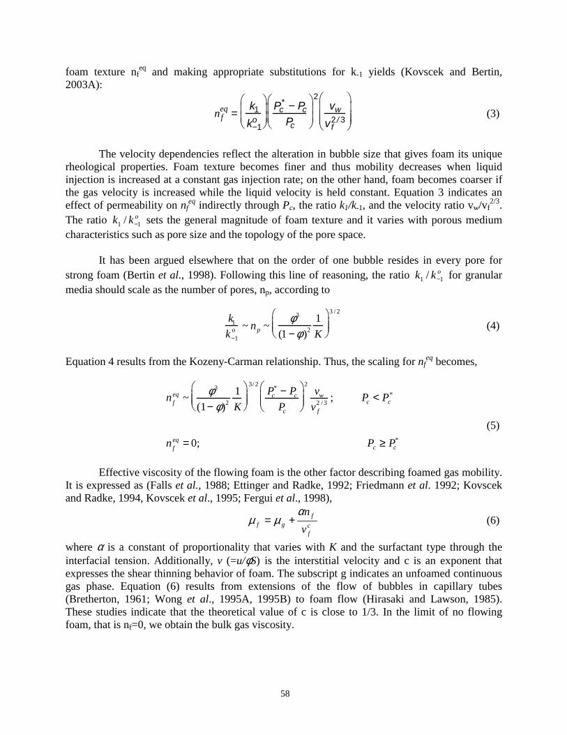
58

foam texture nfeq and making appropriate substitutions for k-1 yields (Kovscek and Bertin,

2003A):

nf

eq =k1

k−1o

Pc* − PcPc

2vw

vf2 / 3

(3)

The velocity dependencies reflect the alteration in bubble size that gives foam its uniquerheological properties. Foam texture becomes finer and thus mobility decreases when liquidinjection is increased at a constant gas injection rate; on the other hand, foam becomes coarser ifthe gas velocity is increased while the liquid velocity is held constant. Equation 3 indicates aneffect of permeability on nf

eq indirectly through Pc, the ratio k1/k-1, and the velocity ratio vw/vf2/3.

The ratio okk 11 / − sets the general magnitude of foam texture and it varies with porous mediumcharacteristics such as pore size and the topology of the pore space.

It has been argued elsewhere that on the order of one bubble resides in every pore forstrong foam (Bertin et al., 1998). Following this line of reasoning, the ratio okk 11 / − for granularmedia should scale as the number of pores, np, according to

k1

k−1o ~ np ~

φ3

(1 −φ)21K

3 / 2

(4)

Equation 4 results from the Kozeny-Carman relationship. Thus, the scaling for nfeq becomes,

nfeq ~ φ3

(1− φ)21K

3/ 2Pc

* − Pc

Pc

2vw

v f2 / 3 ; Pc < Pc

*

nfeq = 0; Pc ≥ Pc

*

(5)

Effective viscosity of the flowing foam is the other factor describing foamed gas mobility.It is expressed as (Falls et al., 1988; Ettinger and Radke, 1992; Friedmann et al. 1992; Kovscekand Radke, 1994, Kovscek et al., 1995; Fergui et al., 1998),

cf

fgf v

nαµµ += (6)

where α is a constant of proportionality that varies with K and the surfactant type through theinterfacial tension. Additionally, v (=u/φS) is the interstitial velocity and c is an exponent thatexpresses the shear thinning behavior of foam. The subscript g indicates an unfoamed continuousgas phase. Equation (6) results from extensions of the flow of bubbles in capillary tubes(Bretherton, 1961; Wong et al., 1995A, 1995B) to foam flow (Hirasaki and Lawson, 1985).These studies indicate that the theoretical value of c is close to 1/3. In the limit of no flowingfoam, that is nf=0, we obtain the bulk gas viscosity.

59

The work of Hirasaki and Lawson (1985) teaches about the permeability dependence of α.After appropriate substitution into Eq. 6 and simplification, we obtain the following scaling forthe effective viscosity of a foamed gas phase:

µ f ≅ nfR3

Rc

1

vf1 / 3

≅β3 / 2K3 / 2Pc

2σnf

v1/ 3(7)

where the capillary pressure, Pc, is recognized as equal to 2σ/Rc. Comparison of Eq. 2 with Eq. 6teaches that α scales as K3/2Pc indicating that the effective viscosity of a foamed gas at fixedtexture and velocity will increase as permeability and capillary suction increase. Falls et al.(1988) also describe a K3/2 dependence for effective viscosity.

Scaling of Foam Mobility

Substitution of Eqs. 6 and 2 into Eq. 1 completes the exercise to obtain the scaling trendsfor foam mobility. The expression reads

λ f =ψ 3K 1+aηkrgo (1−φ)2

φ3

3(1+aη ) / 2Pc

Pc* − Pc

2(1+aη )1

Pc

v f1+2aη / 3

vw1+aη

∇ paη ; Pc < Pc

*

λ f = λg ; Pc ≥ Pc*

(8)

where the terms a and η arise from the exponent model for gas relative permeability and thepercolation network scaling of Sf near the percolation threshold. The proportionality constant ψ3is composed primarily of surface tension and the proportionality constant β.

While quite involved, Eq. 8 incorporates all of the features that foam flow in porousmedia has exhibited. For instance, foam mobility is large if the surfactant is weak or ifconcentration is low through the term including Pc

*. Conversely, foam mobility is low if Pc* is

large. The experimentally observed trend that λ f increases with vf while liquid injection rate isheld constant is found (c.f., Ettinger and Radke, 1991; Persoff et al., 1991; Kovscek et al., 1995).Similarly, λ f varies inversely with increasing vw when gas injection rate is fixed. To expectfunctional dependencies simpler than given in Eq. 8 is naïve given the complex rheologydisplayed by foam.

Table 1. Properties of the Porous Media

high permeability low permeabilityK (µm2) 5.35 0.686

φ 0.395 0.244Swc 0.10 0.25

60

Table 2: Parameters for Gas-mobility Calculations

parameter value capillary pressureµw 1 mPa s

Pc = σ φK

1.4171− SwD( )(−2.1201− SwD( )2

+1.2631− SwD( )3 σ 32 mN/m

wc

wcwwD S

SSS−−=

1a 2.5η 0.4

Pc* 20 kPa

It must be noted, however, that this particular scaling of foam mobility is unlikely toapply to carbonates in a quantitative sense. Equation 4 originates from sands and np cannot bescaled in the same way for carbonates, or high-porosity porous media. Nevertheless, the idea thatthe ratio of foam germination to termination sites scales as the number of pores should remaintrue. For rocks that do not follow Eq. 4, an appropriate relationship can be substituted and theremainder of the exercise repeated.

Consider, briefly, trends for heterogeneous porous media as predicted by Eq. 8. It suggeststhat foam mobility increases with permeability to a power greater than 1 if all other factors arefixed. This is counter to the goals of fluid diversion. Fortunately, the remaining terms teach us theconditions where foam is an effective mobility control and diversion agent.

Next consider the role of porosity on foam mobility through a simple calculation. Wechoose the conditions in Table 1 for representative high and low permeability strata along with aPc

* equal to 20 kPa, an Sw,ss in the sandstone of 0.5, and an Sw,A10 of 0.16. Parameter values arephysical and result from experiments discussed in relation to the experiment to follow. Capillarypressure is obtained from the Leverett J-function and dimensionalizing by the ratio σ(φ/K)1/2.Table 2 summarizes other relevant parameter values. Also for the sake of highlighting the role ofporosity, we set the liquid and gas velocity, as well as the pressure drop, equal in each layer. Theporosity of the high permeability medium is held fixed while the porosity of the lowerpermeability rock is varied from 0.15 to 0.40. The ratio of the gas mobility in the low upon highpermeability layer is then computed according to Eq. 8. The result is given in Fig. 2. When theporosity is about the same as in both media, λf,low/λf,high is less than 1 indicating that diversion isnot expected. Around φ equal to 0.35 the ratio is unity. As the porosity of the lower permeabilitymedium decreases, the ratio λf,ss/λf,A10 increases. This result occurs because the first term inparenthesis on the right of Eq. 8 increases as porosity decreases. Recall that this term originatesfrom the scaling of foam germination and termination sites. For most sands and sandstones,permeability decrease correlates with porosity decrease. Thus, 32 /)1( φφ− counteracts thereduction in mobility indicated by the superlinear scaling of λf with permeability. In cases wherethe porosity contrast is large, the term 32 /)1( φφ− indicates that it should be relatively easy toobtain foamed gas injection into low permeability zones.

61

0.1

1

10

100

0 0.1 0.2 0.3 0.4 0.5porosity in sandstone

Figure 2. Ratio of gas mobility in low and high permeability zones. Porosity oflow permeability layer is varied and all other terms held constant.

Experimental

An experimental setup was prepared to characterize foam flow in individual homogeneouscores and then to consider gas mobility in the composite system as shown in Fig. 3. The porousmedia were A-10 (US Filtration Co.) a high permeability, consolidated, synthetic rock andVosges sandstone. The A-10 is pure silica while the Vosges sandstone contains some claymaterial. Table 3 lists the properties and dimensions of each core. The permeability contrast wasabout 8 to 1, whereas the porosity contrast was roughly 2 to 1. The different cross-sectional areasgave roughly similar pore volume within each core.

The cores were prepared by affixing an aluminium plate to each end via a clamp. Theplates contain ports for fluid injection/production and pressure measurement. The bare rocksurfaces were coated with Araldite 2013 (Ciba Specialty Chemicals) a metal bonding adhesivethat is viscous, nonwetting to silica, and so does not penetrate the rock matrix. Likewise, thisadhesive bonds the metal plate to each face of the core. After drying for 24 hours, the length ofeach core was wrapped with epoxy-coated fiberglas twine to add mechanical strength. Thissystem can withstand absolute pressures of about 500 KPa. We chose to work with cores thatcommunicate only through inlet and exit conditions to more easily characterize the mobility

62

within each porous medium. The effect of capillary communication and cross flow among porousmedia is considered experimentally in another paper (Bertin et al. 1999).

Figure 3. Apparatus for heterogeneous foam-displacement experiments. The mass flow meteris removed if foamer solution is injected.

The aqueous foamer solution was composed of potassium iodide (KI) and Witconate AOS38 (Witco), an α-olefin sulfonate with carbon chain length of 14 to 16. Surfactant concentrationwas 0.2 wt% active chemical in a brine of 1 wt% KI. The CMC is approximately 0.01 wt% andsurface tension is 32 mN/m. Solution viscosity is 1 mPa s. Cores were saturated with foamersolution by first injecting bone-dry CO2 to displace and/or evaporate any fluid. Dryness wasassured by measuring core weight. From 5 to 10 PV of foamer solution were then injected tosatisfy rock adsorption and dissolve any residual CO2. Measurement of rock permeability to thefoamer solution provided a check that there was no residual gas in the system.

Bottled nitrogen was the gas source for foam displacement. Total gas injection wascontrolled using a 0-5 SCCM (standard cubic centimeters per minute) mass flow controller(Bronkhorst). The gas stream was split using a tee and the flow resistance in each porous mediumset the fraction of gas injected into each core. In experiments with injection of only gas, theportion of the gas injected into the sandstone is measured by a mass flow meter (Bronkhorst).Atmospheric back pressure was applied and the production streams were not mingled. Theeffluent from each individual core was collected and measured as a function of time. Pressuretransducers (0 to 100 KPa, Rosemount) measured the pressure drop across each core and a PCrecorded individual measurements.

63

Table 3. Properties of the Porous Media

A-10 Vosges sandstoneK (µm2) 5.35 0.686

φ 0.395 0.244L (m) 0.48 0.497

cross-sectional area (m2) 1.96x10-3 2.62x10-3

pore volume (m3) 3.72x10-4 3.18x10-4


Several injection conditions were imposed. First, gas alone was injected into thecomposite system. No restrictions were placed on the gas injection; each porous mediumaccepted a portion of the injected gas according to the foamed-gas mobility within the core. Thisserved as a confirmation of the diversion properties of foam measured in a separate study (Bertinet al., 1999) with a substantially different apparatus and porous medium geometry. Second,foamer solution and gas were coinjected simultaneously. This was done so as to verify the liquidvelocity dependence in Eq. 24 of Kovscek and Bertin (2001). Finally, the pressure response ofeach individual core to simultaneous injection of gas and liquid was measured so as to establish abaseline.

The porous media are fully saturated with surfactant solution and nitrogen is injected at1.5 SCCM (25 mm3/s). The production from each core is measured as is the pressure drop. In thisexperiment, a mass flow meter is used downstream of the mass flow controller at the inlet of thesandstone to measure the fraction of gas accepted by the sandstone. Comparison of injected gasrate and the measured collection of effluent serve as a mutual check for accuracy. Figure 4presents the pressure response accompanying gas injection and Figure 5 the liquid production.The maximum pressure drop measured over the system is a little more than 0.3 bar (30 kPa) andis relatively low because liquid is not injected into both of the porous media. The steady increasein pressure drop at all times prior to breakthrough is indicative of foam generation and control ofgas mobility. Breakthrough occurs first in the sandstone at 0.7 PV (318 min). At roughly 0.71 PV(328 min), foam begins to exit the A10. After gas production begins, the experimental systemapproaches a pseudosteady state pressure drop as the cores gradually dry out. Gas was injectedfor several hours after breakthrough, but collapse of the foam never occurred. The average watersaturation of each core was calculated from the liquid effluent collected. At breakthrough, Swaverages 0.16 in the A10 and 0.50 in the sandstone.

64

0

0.1

0.2

0.3

0.4

0 0.2 0.4 0.6 0.8 1

time (PV)

sandstoneA10

Figure 4. Pressure drop results for gas-only injection into heterogeneous system.

65

0

0.2

0.4

0.6

0.8

1

0 0.2 0.4 0.6 0.8 1time (PV)

A10sandstone

Figure 5. Liquid production from each core for gas only injection into heterogeneous system.

Because no liquid is injected, we measure the gas injection rate into each core as afunction of time. Figure 6 presents the gas Darcy velocity at the inlet to each core. Initially, gasis more mobile in the higher permeability A10 and it accepts a greater fraction of the injection.Gradually, gas mobility in the A10 drops so that the sandstone accepts a greater fraction of theinjected gas. The excellent diversion of gas to the sandstone despite a contrast in permeability ofalmost 8 to 1, can be explained through the ratio of gas mobility in the sandstone upon that in theA10, λf,ss/λf,A10, computed with Eq. 8. The measured absolute permeability and porosity of eachcore are taken from Table 3. Capillary pressure is computed from the Leverett J-function anddimensionalized according to σ(φ/K)1/2 (see Table 2 of Kovscek and Bertin, 2001). The limitingcapillary pressure is set to 20 kPa according to the work of Apaydin and Kovscek (2001) whoemployed a similar surfactant solution. Next, the gas velocity in each porous medium at gasbreakthrough is taken from Fig. 6 and converted to interstitial velocity using the average gassaturation at breakthrough. That is, Sg is set to 0.5 for the sandstone and 0.85 for the A10. Withthe assembled information and Eq. 8, λf,ss/λf,A10 is equal to 0.868 (vw,A10/vw,ss)1+aη atbreakthrough. Thus, before consideration of liquid velocity effects, we expect gas mobility tohave the possibility of being roughly equal in each porous medium. This agrees well with theexperimentally observed trend that λf,ss/λf,A10 is of order 1 as shown in Fig. 6.

66

0

0.25

0.5

0.75

1

0 0.2 0.4 0.6 0.8 1time (PV)

0

0.2

0.4

0.6

0.8

sandstone (m/day)A10 (m/day)gas mobility: sandstone / A10

Figure 6. Gas Darcy velocity at the inlet to each core and the apparent ratioof sandstone to A10 gas mobility.

In the next set of experiments, gas and foamer solution are injected simultaneously. As inthe previous experiments, the pore space is fully saturated with surfactant solution initially. Thetotal liquid flow rate is 9 mL/hr (2.5 mm3/s) and the gas rate is again 1.5 SCCM (25 mm3/s) as inthe prior gas-only injection. The overall gas fractional flow is 0.90. Each core accepts whateverportion of the injected fluid it desires and, thus, the fraction of gas and liquid entering each core isvariable over the duration of the experiment. Unfortunately, we do not possess a means toquantify the gas fractional flow entering each core. However, transparent tubing connected thevarious flow devices at the inlet of the apparatus and qualitative observations were possible.

Figure 7 displays the pressure response of the system. It exceeds that of the previousexperiment because liquid is coinjected. Gas breaks through in the sandstone at 0.43 PV (180min). At this point, the pressure drop across the system is 0.5 bar (50 kPa). The initial pressureresponse and steady increase of pressure accompanying gas injection again indicate foamgeneration and mobility control of the gas. Gas production from the A10 never occurs, even aftergreater than 10 PV (4200 min) of injection. After breakthrough in the sandstone, pressureincreases steadily, but much more slowly. It reaches a plateau of approximately 1.4 bar (140 kPa)at roughly 9.5 PV of total injection. After breakthrough, the pressure drops measured across each

67

porous medium are not equal. This is probably a capillary effect. Because gas never breaksthrough in the high-permeability A10, a gas-phase pressure is measured on the upstream sidewhile on the downstream side a liquid-phase pressure is measured. After breakthrough in thesandstone, gas is present on both the upstream and downstream sides. Nevertheless, the rate ofpressure increase is the same for each medium and the difference in pressure between the twomedia after breakthrough is virtually constant.

0

0.2

0.4

0.6

0.8

1

1.2

1.4

1.6

0 2 4 6 8 10time (PV)

sandstoneA10

Figure 7. Pressure drop results for simultaneous gas and liquid injection intoheterogeneous system.

The produced liquid from each porous medium as a function of time is presented in Figure8. Initially, the sandstone accepts very little gas. As verified visually, the major portion of the gasenters the more permeable A10 at very small times. Once foam is generated in the A10, gas isdiverted to the sandstone and production of liquid from the sandstone increases. At this stage, thesandstone accepts an increasing fraction of the gas, very little of the injected liquid, andproduction of liquid is fairly efficient. Visual estimates place the gas fractional flow at the inlet ofthe sandstone in excess of 99.9% (one part in a thousand is liquid), at this stage. In contrast theA10, accepts a greater fraction of liquid and a lesser fraction of gas. The production rate from theA10 drops. The system reaches a state where the higher permeability layer is virtually blocked togas flow. The majority of the injected gas enters the sandstone. Liquid production from the A10is rather steady and exceeds 1 because of the continuous liquid injection into the system.

68

0

0.2

0.4

0.6

0.8

1

0 1 2 3 4 5

time (PV)

A10

sandstone

Figure 8. Liquid production from each core for simultaneous injection of gas and liquid intoheterogeneous system.

Mass balance gives the average water saturation of the sandstone at breakthrough equal to0.5, assuming negligible liquid injection. This is identical to the experiment with injection of onlygas. After breakthrough, the fraction of liquid entering the sandstone increases somewhat andvisual estimates place the gas fractional flow between 95 and 99%. This is consistent with theincrease in pressure drop after gas breakthrough. The increased liquid flow leads to increasedfoam generation and reduced gas mobility as indicated by Eq. 8.

The blockage of the higher permeability A10 can be better understood by considering theliquid velocity dependence in Eq. 8 of Kovscek and Bertin (2001). The liquid velocity exponentis larger than that for the gas velocity. Because the A10 accepts most of the injected liquid, theliquid velocity is relatively high within the A10 and the gas mobility is expected to be low. In thiscase, mobility is low enough to lead to blockage of the high permeability core.

Gas-only injection as well as simultaneous surfactant solution and nitrogen injectionexperiments were conducted to contrast with the above heterogeneous experiments. In thesecases, the cores are fully saturated with surfactant solution initially. The rate for gas-onlyinjection is 1.5 SCCM. For coinjection, the gas rate is 1.5 SCCM and the liquid injection rate is0.15 cm3/min.

69

Figure 9 reports the pressure response for the A10 synthetic sandstone. With coinjectionof gas and liquid, the measured pressure drop is about 0.1 bar (10 kPa) greater than without liquidinjection. The dip in both pressure responses at roughly 0.8 PV of injection corresponds to gasbreakthrough. On the other hand, Figure 10 gives data for similar experiments conducted in theVosges sandstone. Here, the pressure drop for coinjection far exceeds that of gas-only injection.Gas breakthrough in the sandstone is at slightly more than 0.5 PV for the gas-only case, whilebreakthrough occurs at roughly 0.7 PV when gas and surfactant solution are coinjected. At 0.7PV, the pressure drop during coinjection is already 0.7 bar, whereas the pressure drop in the gas-only case is about 0.4 bar. Hence, the difference between gas-only injection and coinjectionappears to be more significant in the case of lower permeability porous media. We also note thatthe relatively slow increase in pressure drop after breakthrough during coinjection might bediagnostic of an end effect (Apaydin and Kovscek, 2001).

0

0.1

0.2

0.3

0.4

0.5

0 0.5 1 1.5 2time (PV)

gas only injectioninject gas and surfactant solution

Figure 9. Pressure drop response for gas-only and co-injection into A10 syntheticsandstone.

70

0

0.5

1

1.5

2

2.5

3

0 1 2 3 4 5 6time (PV)

gas-only injection

inject gas and surfactant solution

Figure 10. Pressure response for gas-only and co-injection into sandstone.

It is interesting to contrast the measured pressure drop among the various cases. In thecase of coinjection into the heterogeneous system, the maximum pressure drop is about 1.2 bar(120 KPa). Recall that the sandstone carries all of the injected gas in this case. When this amountof gas is injected along with surfactant solution into the sandstone alone, the overall pressure dropis more than twice as much, 2.5 bar (250 kPa). The chief difference is the amount of liquidflowing in the sandstone in each of these experiments. As Eq. 8 indicates, the gas mobility islower, and the pressure drop correspondingly greater, when the liquid interstitial velocity isgreater.

Conclusions

An experimental and scaling study of foamed gas mobility in heterogeneous porous mediawas performed. The scaling study demonstrated that important factors such as permeability,porosity, capillary pressure, limiting capillary pressure for foam collapse, and liquid and gas

71

velocity can be combined to describe gas mobility upon assumption of local equilibrium of foamgeneration and coalescence rates. Experiments supported predictions of the scaling exercise.Effective diversion of gas to low permeability zones is possible with foam. The experiments alsohighlight the important role of liquid velocity on gas diversion. Foamed gas mobility is inverselyproportional to liquid velocity. A zone of a porous medium that receives the majority of liquidduring coinjection of surfactant solution and gas exhibits low gas mobility. It is within thesezones that the possibility for complete blockage to gas exists.

References

Apaydin, O. and A. R. Kovscek, "Surfactant Concentration and End Effects on Foam Flow inHomogeneous Porous Media," Transport in Porous Media, 43(3), 511-536 (2001).

Bertin, H.J., Quintard, M.Y., and Castanier, L.M.: 1998, Modeling Transient Foam Flow inPorous Media Using a Bubble Population Correlation, Society of Petroleum EngineersJournal 3(4), 356-362.

Bertin, H.J., Apaydin O.G., Castanier, L.M., and Kovscek, A.R.: 1999, Foam Flow inHeterogeneous Porous Media, Society of Petroleum Engineers Journal 4(2), 75-82.

Bertin, H.J.: 2000, Foam Diversion Modeling Using a Bubble-Population Correlation, ,Proceeding of the SPE/DOE Symposium on Enhanced Oil Recovery, Tulsa, OK, U.S.A.,SPE 59366.

Casteel, J.F. and Djabbarah, N.F.: 1988, Society of Petroleum Engineers Reservoir Engineering3, 1186-1192.

Chambers, K.T. and Radke, C.J.: 1991, Capillary Phenomena in Foam Flow Through PorousMedia, in Interfacial Phenomena in Petroleum Recovery, Morrow, N.R. ed., 191-255,Marcel Dekker, NY.

Cheng, L., Kam, S. I., Delshad, M., and Rossen, W.R.: 2001, Simulation of Dynamic Foam-AcidDiversion Process, Proceedings of the SPE European Formation Damage Conference,The Hauge, Netherlands, SPE 68916.

Cohen, D., Patzek, T.W., and Radke, C.J.: 1997, Onset of Mobilization and the Fraction ofTrapped Foam in Porous Media, Transport in Porous Media 28, 253-284.

Corey, A.T.: 1954, The Interrelation Between Gas and Oil Relative Permeabilities, Producer’sMonthly 19, 38-41.

de Gennes, P. G.: 1992, Conjectures on Foam Mobilization, Revue De L’Institut Francais DuPétrole 47(2), 249-254.

72

Ettinger, R.E. and Radke, C.J.: 1992, Influence of Foam Texture on Steady Foam Flow in BereaSandstone, Society of Petroleum Engineers Reservoir Engineering 7, 83-90.

Falls, A.H., Hirasaki, G.J., Patzek, T.W., Gauglitz, P.A., Miller, D.D., and Ratulowski, T: 1988,Development of a Mechanistic Foam Simulator: The Population Balance and Generationby Snap-Off, Society of Petroleum Engineers Reservoir Engineering 3, 884-892.

Fergui, O., Bertin, H. and Quintard, M.Y: 1998, Transient Aqueous Foam Flow in Porous Media:Experiments and Modeling, Journal of Petroleum Science and Engineering 20, 9-29.

Friedmann, F., Chen, W.H., and Gauglitz, P.A.: 1991, Experimental and Simulation Study ofHigh-Temperature Foam in Porous Media, Society of Petroleum Engineers ReservoirEngineering 6, 37-45.

Gillis, J.V. and Radke, C.J.: 1990, A Dual Gas Tracer Technique of Determining Trapped GasSaturation During Steady Foam Flow in Porous Media, Proceedings of the 65th SPEAnnual Technical Conference, New Orleans, LA, U.S.A. SPE 20519.

Hanssen, J. E.: 1993A, Foam as a Gas Blocking Agent in Petroleum Reservoirs I: EmpiricalObservations and Parametric Study, Journal of Petroleum Science and Engineering 10,135-156.

Hanssen, J. E.: 1993B, Foam as a Gas Blocking Agent in Petroleum Reservoirs II: Mechanismsof Gas Blockage By Foam, Journal of Petroleum Science and Engineering 10, 117-133.

Heller, J.P.: 1994, CO2 Foams in Enhanced Oil Recovery, in Foams in the Petroleum Industry,Schramm, L.L. ed., 201-234, Amercan Chemical Society, Washington D.C.

Hirasaki, G.J. and Lawson, J.B.: 1985, Mechanisms of Foam Flow in Porous Media: ApparentViscosity in Smooth Capillaries, Society of Petroleum Engineers Journal 25(2), 176-190.

Hirasaki, G.J.: 1989A, The Steam Foam Process, Journal of Petroleum Technology 41(5), 449-456.

Hirasaki, G.J.: 1989B, The Steam Foam Process, Supplement to SPE 19505 Society of PetroleumEngineers, Richardson, TX.

Hirasaki, G.J., Miller, C.A., Szafranski, R., Lawson, J.B., and Akiya, N.: 1997A,Surfactant/Foam Process for Aquifer Remediation, Proceedings of the SPE AnnualTechnical Conference, San Antonio, TX, U.S.A. SPE 39292.

Hirasaki, G.J., Miller, C.A., Szafranski, R., Lawson, J.B., Tanzil, D., Jackson; R.E., Londergan, J.and Mainardus, H..: 1997B, Field Demonstration of the Surfactant/Foam Process forAquifer Remediation, Proceedings the SPE International Symposium on OilfieldChemistry , Houston, TX, U.S.A. SPE 39292.

Jiménez, A. I. and Radke, C.J.: 1989, Dynamic Stability of Foam Lamellae Flowing Through aPeriodically Constricted Pore, in Oil Field Chemistry: Enhanced Recovery andProduction Stimulation, Borchardt, J.K. and Yen, T.F. eds., 460-469, Amercan ChemicalSociety, Washington D.C.

73

Kharabaf, H. and Yortsos, Y.C.: 1998, Pore Network Model for Foam Formation andPropagation in Porous Media, Society of Petroleum Engineers Journal 13(1), 42-53.

Khatib, Z.I., Hirasaki, G.J. and Falls, A.H.: 1988, Effects of Capillary Pressure on Coalescenceand Phase Mobility in Foams Flowing in Porous Media, Society of Petroleum EngineersReservoir Engineering 3, 919-926.

Llave, F.M., Chung, F.T-H., Louvier, R.W. and Hudgins, D.A., 1990, Foams as Mobility ControlAgents for Oil Recovery by Gas Displacement, Proceeding of the 7th SPE/DOESymposium on Enhanced Oil Recovery, Tulsa, OK, U.S.A., SPE 20245.

Kibodeaux, K., Zeilinger, S. C., and Rossen, W.R.: 1994, "Improved Prediction of FoamDiversion in Matrix Acidization," Proceedings of the 69th SPE Annual TechnicalConference, New Orleans, LA U.S.A. SPE 28550.

Kovscek, A.R. and Radke, C.J.: 1994, Fundamentals of Foam Transport in Porous Media, inFoams in the Petroleum Industry, Schramm, L.L. ed., 115-163, Amercan ChemicalSociety, Washington D.C.

Kovscek, A.R., Patzek, T.W., and Radke, C.J.: 1995, A Mechanistic Population Balance Modelfor Transient and Steady State Foam Flow in Boise Sandstone, Chemical EngineeringScience 50(23), 3783-3799.

Kovscek, A.R. and Radke, C.J.: 1996, Gas Bubble Snap-Off Under Pressure Driven Flow inUnconstricted Noncircular Capillaries, Colloids and Surfaces A 117, 55-76.

Laidlaw, W.G., Wilson, W.G., and Coombe, D.A.: 1993, A Lattice Model of Foam Flow inPorous Media: A Percolation Approach, Transport in Porous Media 11, 139-159.

Myers, T.J. and Radke, C.J.: 1999, Transient Foam Displacement in the Presence of Residual Oil:Experiment and Simulation Using a Population Balance Model, Proceedings of the SPEAnnual Technical Conference, Houston, TX, U.S.A. SPE 56412.

Persoff, P., Radke, C.J., Pruess, K., Benson, S.M., and Witherspoon, P.A.: 1991, A LaboratoryInvestigation of Foam Flow in Porous Media at Elevation Pressure, Society of PetroleumEngineers Reservoir Engineering 6, 365-371.

Robin, M.: 1987, Laboratory Evaluation of Foaming Additives Used to Improve SteamEfficiency, Proceedings of the 62nd SPE Annual Technical Conference, Dallas, TX,U.S.A. SPE 16729.

Rossen, W.R.: 1988, Theories of Foam Mobilization Pressure Gradient, Proceeding of the 6th

SPE/DOE Symposium on Enhanced Oil Recovery, Tulsa, OK, U.S.A., SPE 17358.

Rossen, W.R. and Gauglitz, P.A.: 1990, Percolation Theory of Creation and Mobilization ofFoams in Porous Media, American Institute of Chemical Engineers Journal 36(8), 1176-1188.

74

Rossen, W.R. and Zhou, Z. H..: 1996, Modeling Foam Mobility at the Limiting CapillaryPressure, Society of Petroleum Engineeers Advanced Technoloyg Series 3(1), 146-153.

Rossen, W. R. and Lu Q.: 1997, Effect of Capillary Crossflow on Foam Improved Oil Recovery,Proceedings of the SPE Western Regional Meeting, Long Beach, CA U.S.A., SPE 38319.

Stauffer, D.: 1985, Introduction to Percolation Theory, Taylor and Francis, London.Tanzil, D., Hirasaki, G.J., and Miller, C.A.: 2000, Mobility of Foam in Heterogeneous Porous

Media: Flow Parallel and Perpendicular to Stratification, , Proceedings of the SPE AnnualTechnical Conference, Dallas, TX U.S.A. SPE 63228.

Yaghoobi, H. and Heller, J.P.: 1996, “Effect of Capillary Contact on CO2-Foam Mobility inHeterogeneous Core Samples,” Proceedings of Permian Basin Oil and Gas RecoveryConference, Midland, TX, U.S.A. SPE 35169.

Zehrboub, M., Ben-Naceur, K., Toubol, E., and Thomas, R.: 1994, Matrix Acidizing: A NovelApproach to Foam Diversion, Society of Petroleum Engineers Production & Facilities,May, 121-126.

Zeilinger, S. C., Wang, M., Kibodeaux, and Rossen, W.R.: 1995, Improved Prediction of FoamDiversion in Matrix Acidization, Proceedings of the SPE Production OperationsSymposium, Oklahoma City, OK U.S.A. SPE 29529.

Zhou, Z. H. and Rossen, W. R.: 1992, Applying Fractional-Flow Theory to Foams for Diversionin Matrix Acidization, Proceedings of the 67th Annual SPE Technical Conference andExhibition, Washington D.C. U.S.A. SPE 24660.

Zhou, Z. H. and Rossen, W. R.: 1992, Applying Fractional-Flow Theory to Foam Processes at the"Limiting Capillary Pressrue", Proceedings of the SPE/DOE 8th Symposium on EnhancedOil Recovery, Tulsa, OK. U.S.A. SPE 24180.

75

Thermally Induced Fines Mobilization and Wettability

(Task 1c)

Introduction

Thermal recovery research and field operations indicate that reservoir rock exposed tohigh temperature undergoes a systematic shift in wettability toward water wetness (Bennion andThomas, 1992; Al-Hadhrami and Blunt, 2001). The consequence of a shift toward water wetnessis that steam and steam condensate become more effective displacement agents and the rockmatrix imbibes water more effectively. It is well understood that wettability influences the flowand relative permeability characteristics of porous media (Bennion and Thomas, 1992; DiCarlo etal., 1998). Examination of temperature as a variable on relative permeability has been conductedsince the 1960's (Edmonson, 1965; Poston et al., 1967; Sinnokrot et al., 1969). The effects offluid properties, such as pH and salinity, on fines migration and permeability are discussedextensively in the formation damage literature (Young, 1979; Kia, 1987; Zhou et al., 1997;Vaidya and Fogler, 1990; Gunter et al., 1992). Yet, controversy exists regarding the origin oftemperature effects and their extent. To date, no plausible mechanism describes this shift towardwater wetness. Fines mobilization presents one pathway to create fresh water wet surfaces.

In order to understand the mechanisms of fines mobilization, we review and use DLVO(Derjaguin, Landau, Verway and Overbeek) theory. It explains the stability of colloidal systemsas a result of the balance of attractive and repulsive forces. As will be shown, DLVO calculationspredict a profound effect of temperature on fines stability. Release of fine clay material ispredicted at conditions (pH, salinity, temperature) obtained during steamflood. Predictions arepresented in the form of isotherm maps. They are confirmed experimentally by core waterfloodsperformed in Berea sandstone at temperatures ranging from 20 to 200°C. Permeability reductionis observed with temperature increase and fines mobilization occurs repeatably at a particulartemperature that varies with solution pH and ionic strength. A scanning electron microscope(SEM) was used to analyze composition of the effluent samples collected during experiments.This study shows that temperature is a decisive factor in fines release and the temperature atwhich the detachment of fines occurs is well predicted by DLVO theory.

Discussion of this topic is organized in the following fashion. First a scenario forwettability alteration at elevated temperature is given. Second, corefloods with hot water are usedto show that temperature mobilizes fines in Berea sandstone. Third, surface forces, so calledDLVO theory, are used to explain experimental observations.

Wettability Alteration

The mechanism for formation of mixed wettability in initially water-wet rocks that hascome to be accepted in recent years is that asphaltenes are deposited on pore walls when aqueouswetting films coating solid grains are unstable (Kovscek et al., 1993). This mechanism explainsthe formation of continuous oil-wet pathways on pore walls and the origin of oil-wet and water-

76

wet surfaces within the same core (Kovscek et al., 1993). For all practical purposes, asphaltenesadhere irreversibly to siliceous or carbonaceous surfaces. Solvents such as hot pyridine arerequired to remove asphaltene from solid material (Windholz et al., 1976).

A possible scenario for wettability shift toward water wetness as a function of finesdetachment is shown in Fig 1. Figures 1.1.a, 1.2.a and 1.3.a represent mixed-wet systems withoil-wet fines attached to the matrix wall at initial reservoir temperature for three different initialscenarios; before (Fig. 1.1.a), during (Fig. 1.2.a) and after (Fig. 1.3.a), waterflood is performed.Dark shading denotes oil; whereas water is lightly shaded. Brackets located outside of thetriangular pore indicate the section of the pore wall that is oil-wet.

Figure 1. Triangles in 1.a through 3.b illustrate pore spaces. Gray color symbolizes the water phase, black color designates oil phase and, round white circles represent clay particles.

The same pore systems in Figs. 1.1.a, 1.2.a, and 1.3.a are represented at greatertemperatures, in Figs. 1.1.b, 1.2.b, and 1.2.c, respectively. In all three figures, an increase oftemperature is hypothesized to cause the detachment of fines from the walls. The grainsunderlying the fines are water-wet because oil never contacted them directly. The fraction ofwater-wet surface thereby increases. Thus, Fig 1.1.b represents a system with greater connatewater saturation that has shifted to water wetness as a result of temperature increase. In Fig. 1.2.bwe represent another possible scenario where fines detach from a portion of the wall. In this case,the shift to water wetness occurs in the area where the fines are exposed to water that has imbibedspontaneously. Fines detached from the wall could be present in both water and oleic phases. Thispossibility explains the existence of fines in water effluent reported by some authors (Tang andKovscek 2002). In Fig. 1.3.b, there is also detachment of the fines from the pore walls duringforced imbibition. Thus, Fig 1.3.b. represents a system with lower residual oil saturation andincreased water wetness.

77

Fines release and change in wettability, illustrated in Fig. 1, may occur under particularfluid conditions (pH, salinity, composition) and characteristics of the mineral surface. Thismechanism is invalidated immediately if temperature cannot be shown to cause the release offines from solid surfaces. Our next step is to conduct experiments that illustrate fines mobilizationat elevated temperature.

Experimental Investigation

We designed experiments to (a) validate the hypothesis that temperature is crucial in finesrelease and, (b) map the sensitivity of the conditions to the temperature. The rock samples areBerea sandstone (Cleveland Quarries). The advantages of using Berea sandstone include theconsiderable amount of clays and, its large permeability that allows experiments to be performedin a relatively short time.

Figure 2(a) shows an image of the Berea Sandstone used, magnified at 250X with ascanning electron microscope (JEOL JSM-5600 LV). Note the fine material adhering to the sandgrains. The area enclosed by the square was magnified 5000 times and it shows the classic plate-like or, accordion-like mineral form of kaolinite

x250

x5000

(a)

(b)

Figure 2. SEM images from Berea sandstone core used in experiments.(a) before and, (b) after waterflood.

We performed 20 tests with unfired cores and 3 tests with a fired core. The cores weresubject to single-phase water injection at different pH, salinity, and temperatures. The salinity andpH of each of the injection fluid is listed in Table 1.

78

Figure 3 shows the layout of experimental apparatus. The cores were cylindrical withlength between 4 and 6 cm and diameter of 2.5cm. Core porosity ranged between 20 and 23 %.Cores were placed in vacuum and temperature of 50 °C for a minimum of ten hours. Theapparatus is assembled by coating the core with a thin film of solvent resistant sealant (FluoroSilicone Rubber) and placing the core inside FTP heat-shrink tubing (Plastic Professional). Thiscovering serves as a high temperature sleeve. A net confining pressure of approximately 250–400psia is applied. The cores were subject to waterflood at different conditions. Corefloods wereperformed at constant Darcy velocity of approximately 1.0 m/day. This injection flow rate istypical for fluid injection and, small enough to prevent “wormholes” at high temperatures.

Berea sample

backpressure

PressureTransducer

oven

Pump

Co nfining pressure

k=100-250 md

φφφφ= 20%

Fixed flow rate 1 m/day

Figure 3. Experimental apparatus.

Experiments were performed at a variety of temperatures, salinities, and pH, underisothermal conditions. The core holder is placed in the oven ( Blue-M thermostated to ± 1ºF ) forwaterflood at high temperature. Back- pressure is used in order to ensure single phase flow insidethe core at high temperature. The pH of the solutions in all experiments was adjusted andcontrolled by using buffers. We used a buffer consisting of sodium hydroxide and potassiumphosphate for pH 7. A solution of sodium bicarbonate and sodium carbonate was used for analkaline pH of 10. Cores were flushed with a copious amount of buffer solution prior totemperature to satisfy any losses of buffer to the rock.

Flow rate was held constant and, changes in permeability were observed by measuring thepressure drop across the core. Fines migration was verified by collecting effluent samples fromexperiments. Some effluent solutions were filtered and analyzed to verify the presence of clays.

The first experiment validated both the experimental setup and procedure. Also, thisexperiment verified that fines production was possible from this set of cores. In the first

79

experiment, a core was subjected to 10-4 M NaCl solutions at 25°C. Initially, the core wasexposed to a high salinity solution (1 M NaCl) and permeability was allowed to stabilize. Thecore was then exposed to low salinity solution (10-4 M NaCl). As the low salinity solution wasinjected, the core suffered an abrupt reduction of permeability to about 1% of the initialpermeability and fines were observed in the effluent. The effluent collected during the injectionof low salinity solution was analyzed using backscattered electron microscopy (BSE-SEM).Backscattered electron images give contrast based on atomic number and provide compositionalinformation. Material with a greater atomic number appears brighter than lower atomic numbermaterial. X-rays are produced as a by-product of the interaction of the SEM electron beam withthe atoms in the sample surface. These X-rays have energies that are characteristic of the atomsthat produce them. Furthermore, the number of X-rays produced by the atoms of a particularelement is related to the concentration of that element in the sample being scanned.

Table 1: Summary of Experimental Conditions.

Figure 4 shows the composition obtained from the filtered material. Aluminum andsilicon are present in large proportion indicating clays in the sample collected. The presence ofpotassium (K) might indicate the presence of illite (Hower, 1974).

80

Figure 4. Compositional chromatography of effluent fines collected (low salinityinjection, test # 2 in core #1, pH=7, 0.01 M NaCl).

The next experiments were performed at constant salinity and pH conditions, withchanges in the temperature. Tests run in cores 2 and 3 compared two systems with identical brineconcentrations but different pHs (7 and 10). Experiments in cores 3, 4, and 5 compare threesystems with the same alkaline pH, but different brine concentrations. Experiments in cores 4 and6 compare the effects of fired core versus unfired core. Finally, further tests, performed in cores 7and 8, were conducted to establish repeatability. The selection of an alkaline pH comes from theobservation that steam condensates have large pH typically ranging from 10 to 12 (Gunter et al.,1992).

The initial permeability for all experiments was calculated at room temperature. Afterstabilizing flow, temperature was increased to 80°C (353 K), 120°C (353 K), and 180°C (453 K),sequentially. Permeability and fines release were monitored continuously.

Figure 5 summarizes the permeability variation observed in each of the experimentsperformed. Open symbols indicate that the fluid collected was fine-free while filled symbolsdenote the presence of fines in the effluent. Identical symbols for different tests indicate testsperformed at identical conditions. In all experiments, the cores that were not fired sufferedreduction in the permeability as we increased the temperature. The permeability reduction mightindicate the presence of swelling clays or that fine release occurs, but they do not mobilize.Nevertheless, the greatest reduction in permeability is associated with conditions that producefines in the effluent.

Effluent collected from test # 3 in core 2 was filtered and analyzed with the SEMtechnique. Figure 6 shows the texture image of a portion of the filter. In texture images, brighterobjects are more distanced from the mean surface of the image. Compositional analysis of brightparticles in Fig. 6 shows much silicon and aluminum among other elements. The fines producedare most likely the pore lining clays illustrated in Fig. 2(a). Figure 2(b) shows a portion of core 2after test # 3 was completed, the pore surface appear to be free of fines relative to Fig. 2(a).

81

Figure 5. Permeability change during experiments. Open symbols indicate no fines in effluent, whereas closed symbols indicate fines production.

Figure 6. View of the filtrate collected during test 3 (120°C) from core 2.Bright portions have large density.

82

Experiments performed in cores 3, 4, and 5 compare the behavior of systems with alkalinepH for different salinity. As we increased the sodium chloride concentration, the reduction inpermeability is less severe. None of the tests performed on core 5 produced fines. Hot waterfloodperformed on the fired core 6 shows a slight increase of permeability as we increased thetemperature opposed to the behavior of the rest of experiments. No fines production was observedfrom the fired core. The contrast of results between tests in cores 4 and 6 confirmed that once thestabilization of clays in the rock is achieved by means of high salinity, the increase in temperaturedid not induce the detachment of fines. Finally, experiments performed in cores 7 and 8 repeatedresults and the observations made in similar tests performed on cores 5 and 4, respectively.

Surface Forces

In order to understand the relationship of the experimental variables with temperature and,predict fines detachment with increase in temperature, we invoke surface forces theory. Surfaceforces are generally mentioned in research concerning formation damage associated withpermeability impairment due to fines migration (Bennion and Thoma, 1992; Young, 1979; Kia,1987; Zhou et al., 1997; Vaidya and Fogler, 1990; Gunter, 1992). Surface forces are alsoincluded in studies that link wettability with fluids composition, salinity and pH (Kovscek et al.,1993; Melrose, 1982; Takamura and Chow, 1983; Anderson, 1986; Churaev, 1988;Buckley et al.,1997; Hirasaki, 1991; Buckley et al., 1996). The focus of these investigations is primarilybetween surfaces forces and properties such as composition, salinity, and pH. Temperature isseldom mentioned.

Forces acting between two charged colloidal particles in an electrolyte solution are eitherattractive (FA) or repulsive (FR). In principle, the stability of colloidal systems is explained by thebalance of these two interactions. The net interaction is either repulsive or attractive. This idea isreferred to as DLVO (Derjaguin, Landau, Verway, and Overbeek) theory. It is assumed thatcolloidal particles are very large compared with electrolyte ions. This makes it possible toexpress the interaction forces between particles, FT, as a function of the interparticle distance, h.

FT (h) = FA (h) + FR(h) (1)

The balance between the forces affecting a clay particle in a reservoir determines the stability ordetachment of the clay particles.

The analysis assumes that a single phase wetting fluid is in contact with the pore surfaceand fines, and it models the system of a fine attached to a pore wall as a simple geometricalobject (sphere, rod, plate), attached to a flat surface, as shown in Figure 7. The interactionbetween a clay particle and a pore surface is described by the following equation,

Vt (h) = VLVA (h) + VDLR (h) +VBR(h) + VHR (h) + VIHL (h) (2)

83

where V is the potential and subscripts represent: t, total; LVA, the London Van Der Waalsattraction; DLR, the double layer repulsion; BR, the Born repulsion, HR, the hydrodynamicrepulsion; and IHL, interfacial hydrate layer. The resulting potential of a clay particle is repulsive(unstable) if Vt is positive and, attractive (stable) if it is negative. The different composites of thisequation and their computation are discussed next.

Figure 7. Sphere-plate system for modeling fines stability.

The London-Van der Waals attractive energy, VLVA(h), acts between interacting bodiesover distances as large as 100 Å. Their magnitudes are comparable to that of the electrical doublelayer. In our system, we neglect the effects due to retardation of electromagnetic waves becausethe ratio of the distance of separation, h, to the particle fines radius, rp, is much less than unity.Thus, the London Van-der Waals potential is estimated numerically by the expression forunretarded interaction (Hamaker, 1937),

VLVA(h) = −A6

2(H +1)H(H + 2)

+ lnH

H + 2

(3)

where, A is the Hamaker constant, and H is the ratio of the distance of separation to particleradius, H = h / rp. In order to proceed, a particle radius of 1 µm is chosen consistent with the SEMimage in Fig. 2. The attractive van der Waals forces are independent of changes in solutionchemistry. The Hamaker constant characterizes the dispersion interaction between the fines andthe pore walls separated by a film of wetting fluid. We estimated this constant using the knownbinary values for kaolinite-water-kaolinite, Akwk, and silica-water-silica, Asws:

kwkswsswk AAA = (4)

The value of the Hamaker constant estimated for the system silica-water-kaolinite is 2.26E-20 J.This is close to the value used by Kia et al. (1987), 2.6E-20 J. We assume the Hamaker constantto be independent of the temperature. Studies of the effect of temperature on the Hamaker

84

constant for ceramic systems report a change of 3% over the range 27 – 200 °C (French 2000),this change is very small considering the changes in the other terms in Eq. 1.

The double layer repulsion term, VDLR(h), is calculated assuming a constant chargecondition as

VDLR(h) =ε rp

4Φ01

2 + Φ022( ) 2 Φ01Φ02

Φ012 + Φ02

2

ln

1+ exp( −κh)1− exp( −κh)

− ln 1− exp( −2κh( )

(5)

where κ is the Debye-Huckel reciprocal length, ε is the dielectric constant of the medium, and Φoiis the surface potential of the wall (i=1) and particle (i=2). Surface potential cannot be measureddirectly but they are approximated by zeta potentials derived from measurements (e.g,electrophoretic mobility).

The Debye-Huckel reciprocal length term is given by

Tne2 b

2

kε=κ (6)

Where nb is the total ion density in bulk. The surface potential of each surface, Φoi, isapproximated by the zeta-potential ζ i, that is the electrical potential at the boundary between the

Stern layer and the diffuse layer. The zeta potential is approximated by the Nernst equation,

ςi = Φoi = −2.3kTe

pH − pHoi( ) (7)

Where pHoi is the isoelectric point of surface i.

The Born repulsion term, VBR(h), measures the short-range molecular interaction resultingfrom the overlap of electron clouds. It is suggested to follow the relationship39

VBR =Aδ6

75608 rp + h

(2rp + h)7 +6 rp − h

h7

(8)

Where δ is the collision diameter. It is assigned a value of approximately 5 Å40. Finally, VHR(h)is the hydrodynamic potential and, VIHL(h) is the interfacial hydrate layer. The effects of thesetwo terms are considered relatively small and can be neglected. Hydrodynamic forces wereestimated for a similar system with flow rates an order of magnitude greater than those used inour experiments. Hydrodynamic forces remain negligible compared to the London-Van derWaals attractive forces (Khilar and Fogler, 1984).

85

Figure 8 illustrates the three main components of a clay-quartz system at roomtemperature, pH of 7, and brine concentration of 0.1 M. In this particular case, the resulting totalpotential is negative and translates into a stable (attractive) system. In order to study the jointeffect of temperature, fluid salinity and pH, we computed a series of such force versus distancecurves. As temperature increases, the minimum in Vt increases approaching the crossover fromattractive to repulsive.


We define the detachment temperature of a fine as the temperature where the resultingpotential, Vt, switches from attractive to repulsive for a given salinity and pH. In the next section,we present the resulting potential for the sphere-plate system for various conditions in quartz-claysystems. Quartz is the most abundant fraction by weight in sandstone and is present largely in theform of sand grains with a lesser fraction present as fines. Clay minerals such as kaolinite andillite are non-swelling clays commonly found in Berea sandstone (Conway et al., 2000) andhydrocarbon producing formations (Hower, 1974; Scheuerman and Bergersen, 1990). As a finalpoint, we assume that the clay surface charge is homogeneously distributed over the sphere.

-1.00E-17

-8.00E-18

-6.00E-18

-4.00E-18

-2.00E-18

0.00E+00

2.00E-18

4.00E-18

6.00E-18

8.00E-18

1.00E-17

0 1E-09 2E-09 3E-09 4E-09 5E-09 6E-09 7E-09 8E-09 9E-09 0.00000

h [m]

Pote

ntia

ls

VDLR(h)

VLVA(h)

VBR(h)

VT(h)

VLVA

VT

VDLR

VBR

Figure 8. Components of sphere-plate interaction and total potential atpH=7 and [Na+]=0.1M.

86

Quartz-Kaolinite System

Kaolinite is a common hydrous alumina silicate. Various zeta potential measurements arefound in the literature (Lorenz, 1969; Williams and Williams, 1978,; Ramachandran andSomasundaran, 1986). We adjust the zeta potentials predicted by Eq. 8 to published values forkaolinite using regression. Figure 9 shows zeta potential as a function of pH at differenttemperatures, for (a) quartz and, (b) kaolinite correspondingly. The points indicate zeta potentialreported (Ramachandran and Somasundaran, 1986) while lines represent the fit curve used in ourmodel. Figure 10 shows zeta potential as a function of pH for quartz and kaolinite, this time at aconstant temperature and various salinity values. We define the change of zeta potential as afunction of temperature, by fitting values of zeta potential for different temperatures(Ramachandran and Somasundaran, 1986). Figure 11 compares the change of zeta potential withrespect to temperature for quartz and kaolinite, by fixing a reference value at room temperature.The values for alumina (Pagneoux et al., 1998), silica (Dai and Chung, 1995), and bitumen (Daiand Chung, 1995) are shown for comparison. According to this plot, all materials follow a similarbehavior with increasing temperature: the zeta potential becomes more negative as thetemperature increases. This observation agrees with other studies (Dai and Chung, 1995).

-150

-100

-50

0

50

0 2 4 6 8 10 12 14 16

pH

Zeta

pot

entia

l, m

V

Experimental, 10 CExperimental, 35 CExperimental, 75 CModel, 10 CModel, 35 CModel, 75 C Model, 120 CModel, 180 C

-60

-50

-40

-30

-20

-10

0

10

20

30

0 2 4 6 8 10 12

pH

Zeta

Pot

entia

l, m

V

Experimental 25 CExperimental 75 CModel, 25 CModel 75 CModel, 120Model, 180 C

Figure 9. Experimental and calculated zeta potential of as a function of pH at constant salinity: (a) Quartz, 1E-3M NaNO3, (b) Kaolinite, E-4M NaCl.

The zeta potentials are used in the calculation of the total potential according to Eq. 2.The total potential tends toward repulsive as the temperature increases. Repeated calculations ofthe total potential for different fluid pH and sodium chloride concentration allows prediction ofthe temperature at which the force between sphere (clay) and plate (grain surface) is no longerattractive. Figure 10 shows contour maps of detachment temperatures for a kaolinite-quartzsystem according to the experimental ζ-potential curve reported by Lorenz (1969) from Fig. 9.

87

Figure 10. Detachment temperature obtained for quartz-kaolinite systems with ζ-potentialmeasurements provided by Lorenz. Shading is in degree Celsius (°C).

The sodium chloride concentrations (salinity) ranges between 0.001 and 0.2 M (100 and12000 ppm) and pH values from 5 to 14. For low salinity and high pH, the resulting potential atroom temperature is mostly repulsive indicating fines release. As we increase pH and decreasesalinity, the detachment temperature decreases. For instance, the system with pH 7 and salinity of0.01 M shows a detachment temperature of approximately 150 °C while the system with pH 10shows a detachment of temperature of only 50°C. This is expected because the zeta potentialbecomes more negative with increasing pH. As a consequence, the force between the clay andsurface becomes repulsive at temperatures only slightly greater than room temperature.

We constructed and compared contour maps for the other two data sets of zeta values(Williams and Williams, 1978; Ramachandran and Somasundaran, 1986). The zeta potentialsdiffer not only with respect to the range of values covered, but also in the isoelectric points. Asexpected, the sensitivity of the system to the bulk conditions depends on the zeta values used inthe calculation. Nevertheless, all calculations predict considerable sensitivity to temperature. Zetapotentials reported by Lorenz (1969) lead to a greater temperature sensitivity as compared to thezeta potentials reported by Williams and Williams (1978) and Ramachandran and Somasundaran(1986). The position of the isoelectric point contributes to the sensitivity to temperature, as well.As the isoelectric point shifts toward the origin, the clay surface becomes negatively charged at alower pH. We considered the isoelectric point to be fixed in all calculations; however, theliterature suggests that the isoelectric point shifts to lower pH as the temperature increases (Daiand Chung, 1995). Such behavior increases the sensitivity to temperature, in some cases.

88

Figure 10 shows contour maps for kaolinite-quartz sytems assuming that fine clays havecylindrical shapes. We use the ζ-potential provided by Lorenz (1969) similar to the calculationsshown in Fig 12. The calculations of the double layer repulsive forces for the cylinder-platesystem used the linear superposition approximation (LSA)(Mahmood et al., 2001, Gregory,1975). The approximation yields results intermediate between constant charge and constantpotential assumptions (Gregory, 1975). Cylinder-plate calculations predict a system moresensitive to temperature than the sphere-plate configuration. For comparison, we also performedcalculations for plate-plate systems. The cylinder-plate and plate-plate systems showed roughlythe same sensitivity to an increase in temperature.

Figure 10 also compares results obtained experimentally to the theoretical calculationsdescribed in this section. Circles indicate that pH and salinity of an experiment whereas theshading of the circle reports the temperatue at which fines were produced with the effluent.Results are mostly in agreement with calculations assuming sphere-plate systems and the ζ-potential provided by Lorenz (1969). Overall, the temperature of fines production is wellapproximated by DLVO theory.

Quartz-Illite System

Illite, a potassium aluminum silicate hydroxide hydrate mineral of the clay group, isanother common clay present in hydrocarbon reservoirs. It is formed during the alteration ofsilicate minerals such as mica and feldspar. Illite is also known as clay mica.

We repeated the calculations applied to the quartz-kaolinite system. The zeta potentialsfor illite (Horikawa, 1988) are more negative than those for kaolinite. Assuming that illite followsthe same reduction in ζ-potential versus temperature function as kaolinite, we calculate thedetachment temperatures. Figure 11 shows the contour map of the detachment temperature for anillite-quartz system. The sodium chloride concentrations (salinity) range between 0.0 and 5 M(100 and 250,000 ppm) and pH values between 5 and 14. The quartz-illite system is moresensitive to changes in temperature. Thus, it is more prone to detachment than the quartz-kaolinite system. The fact that the zeta potentials are more negative results in greater repulsiveforces. The isotherms are almost horizontal indicating that the resulting potential shows the samebehavior for the range of pH at a given salinity.

89

Figure 11. Detachment temperature obtained for quartz-illite system.Shading is in degree Celsius (°C).

Conclusions

The interaction between fluid and surface forces is a dominant factor in wettability andformation damage. Interactions depend on factors including mineralogy of the porous medium,concentration and chemical composition of the fluids, pH, and temperature of the system.Temperature is very little studied in the surface forces literature in relation to fines mobilization.In this work, we develop an understanding of fines mobilization through experiments and the roleplayed by surface forces. Results confirm the decisive role of the interplay of temperature, pH,salinity, and mineralogy on these phenomena. The value of the isoelectric point variessignificantly with the surface mineralogy. This variation is responsible for the sensitivity thatfines show to the change of fluid and temperature conditions. The results presented here taughtthat temperature increase allows fine release under conditions of high pH and moderate salinity.Fines detachment changes the nature of fluid-solid interactions in porous media supporting ourhypothesis that fines mobilization is a mechanism for porous media to shift towards waterwetness during thermal recovery operations.

90

References

Anderson, W. G: “Wettability, Survey-Part 1: Rock/Oil/Brine Interacitons and the Effect of CoreHandling on Wettability,” SPE 13392. Journal of Petroleum Technology, October 1986.Pp 1125-1144.

Al-Hadhrami, H. S. and M. J. Blunt, “Thermally Induced Wettability Alteration to Improve OilRecovery in Fractured Reservoirs,” SPE Reservoir Evaluation and Engineering, June2001, pp 179-186.

Bennion, D. B. and F. B. Thomas: “ Formation damage Due to Mineral Alteration andWettability Changes During Hot Water and Steam Injection in Clay-Bearing SandstoneReservoirs,” SPE paper 23783, proceedings of the SPE International Symposium onFormation Damage Control, held in Lafayette, Louisiana, February 26-2. 1992.

Buckley, J.S., K. Takamura and N.R. Morrow: “Influence of Electrical Surface Charges on theWetting Properties of Crude Oil,” SPE 16964. Proceedings of the 62nd SPE AnnualTechnical Conference and Exhibition, Dallas, TX. September 27-30, 1997.

Buckley, J. S.: ”Asphaltene precipitation and Crude Oil Wetting,” SPE Advanced TechnologySeries, Vol. 3. No. 1. pp 53-59.

Buckley, J. S., C Bosseau, and Yu Liu: “Wetting alteration by Brine and Crude Oil: FromContact angles to Cores,” SPE 30765. SPE Journal, September 1996. pp 341-350.

Churaev, N. V. “Wetting Films and Wetting,” Revue de Physique Appliquée. 23 (1988) No 6. pp975-987.

Conway, M.W., R. E. Himes and R. Gray: “Minimizing Clay Sensitivity to Fresh WaterFollowing Brine Influx,” SPE 58748. Proceedings of the 2000 SPE InternationalSymposium on Formation Damage Control held in Lafayette, LA, 23-24 February 2000.

Dai, Q and K. H. Chung: “Bitumen-sand Interaction in Oil in Sand Processing,” Fuel. Vol 74.No. 12, pp. 1858-1864, 1995.

Diabira, I., L. M. Castanier, and A. R. Kovscek, “Porosity and Permeability EvolutionAccompanying Hot Fluid Injection Into Diatomite,” Petroleum Science and Technology,19 (9&10), 1167-1185 (2001).

DiCarlo, D. A., A. Sahni, and M. J. Blunt, “The effect of Wettabilility on Three-Phase RelativePermeability,” SPE paper 49317, proceedings of the SPE Annual Technical Conferenceand Exhibition, held in New Orleans, Louisiana, 27-30 September 1998.

Edmonson, T. A.: "Effect of Temperature on Waterflooding," J. Cdn. Pet. Tech (Oct-Dec 1965)236-42.

91

French, R. H.: “Origins and Applications of London Dispersion Forces and Hamaker Constants inCeramics,” J. Am. Ceram. Soc., 83 [9] 2117-46 (2000).

Gunter, W. D., Z. Zhou, and E. H. Perkins: “Modeling Formation Damage Caused by Kaolinitefrom 25 to 300 Centigrade In the Oil Sand Reservoirs of Alberta,” SPE 23786.Proceedings of the SPE Intl. Symposium on Formation Damage Control, Louisiana,February 26-27, 1992.

Gregory, J.: “Interaction of Unequal Double Layers at Constant Charge,” Journal of Colloid andInterface Science, Vol. 51, No. 1, April 1975.

Hamaker, H.C.: “The London-Van der Waals Attraction between Spherical Particles,” Physics, 4,1058 (1937).

Hirazaki, G. J.: “ Wettability: Fundamentals and Surface Forces,” SPE 17367. SPE FormationEvaluation, June 1991, pp 217-226.

Horikawa, Y., R. S. Murray and J. P Quirk: “The Effect of Electrolyte Concentration on the ZetaPotentials of Homoionic Montmorillonite and Illite,” Colloids and Surfaces, 32 (1988) pp.181-195

Hower, W.F.: “Influence of Clays on the Production of Hydrocarbons,” SPE paper 4785.Proceedings of the AIME Symposium on Formation Damage Control, held in NewOrleans, LA, Feb. 7-8, 1974.

Khilar K.C. and H. S. Fogler: “Colloidal Induced Fine migration in porous media, Reviews inChemical Engineering, n. 4, 1987, pp 41-108.

Khilar, K. C. and H. S. Fogler: “The existence of a Critical Salt Concentration for ParticleRelease,” Journal of Colloid and Interface Science, Vol. 101, No. 1, September 1984.

Kia, S. F.: “Effect of Salt Composition on Clay Release in Berea Sandstone,” SPE paper 16524.Proceedings of the SPE International Symposium on Oilfield Chemistry. San Antonio,Texas, February 4-6, 1987.

Kovscek, A. R., H. Wong and C. J. Radke: “A pore-Level Scenario for the Development ofMixed Wettability in Oil Reservoirs,” Environmental and Energy Engineering, AIChEJournal, June 1993, Vol. 39, No. 6. pp 1072-1085.

Lorenz, P B. , Clays Clay Miner., 17 (1969) 223-251.

Mahmood, T., A. Amirtharajah, T. W. Sturm and K. E. Dennett: “A Micromechanics Approachfor Attachment and Detachment of asymmetric Colloidal Particles,” Colloids and SurfacesA: Physicochemical and Engineering Aspects 177 (2001) pp. 99-110.

92

Melrose, J.C.: “Interpretation of Mixed Wettability States in Reservoir Rocks,” SPE paper 10971,proceedings of the 57th SPE Annual Fall Technical Conference and Exhibition, NewOrleans, LA, September 26-29, 1982.

Pagneoux, C., M. Serantoni, R. Laucournet, T. Chartier, and J. F. Baumard: “Influence of theTemperature on the Stability on Aqueous Alumina Suspension.” J. Am. Ceram. Soc.,1998. pp 1935 – 1948.

Poston, S. W, S. Ysrael, A. K. M. S. Hossain, E. F. Montgomery and H. J. Ramey, “The effect ofTemperature on Irreducible Water Saturation and relative Permeability of UnconsolidatedSands,” SPE paper 1897, proceedings of the SPE 42nd Annual Fall Meeting, held inHouston, Oct 1-4, 1967.

Ramachandran, R. and P. Somasundaran: “Effect of Temperature on the Interfacial Properties ofSilicates,” Colloids and Surfaces, 21 (1986) 355-369.

Scheuerman, R. F. and B.M. Bergersen: “Injection-Water Salinity, Formation Pretreatment andWell-Operations Fluid-Selection Guidelines,” SPE paper 18461. Journal of PetroleumTechnology, July 1990. pp 836-845.

Sinnokrot, A. A., H.J. Ramey and S.S. Marsden: ”Effect of Temperature Level upon CapillaryPressure Curves,” SPE 2517. Proceedings of the SPE 44th Annual Fall meeting, Denver,Colorado (Sept 28-Oct. 1, 1969).

Takamura, K. and R. S. Chow: “A mechanism for Initiation of Bitumen displacement from OilSand,” Journal of Canadian Petroleum Technology, Nov-Dec 1983, pp 22-30.

Tang, G. and A. R. Kovscek, "Wettability Alteration of Diatomite Induced by Hot-FluidInjection," SPE paper 77461, the proceedings of 2002 Annual Technical Conference andExhibition, held on 29 September to 2 October, 2002 in San Antonio, TX

Tang, G. and N. R. Morrow, “Influence of brine composition and fines migration on crudeoil/brine/rock interactions and oil recovery,” Journal of Petroleum Science andEngineering 24 (1999) 99-111.

Tang, G. and A. R. Kovscek, “Experimental Study of Heavy Oil Production from Diatomite byWater Imbibition at Elevated Temperatures,” Proceedings of the SPE/DOE ThirteenSymposium on Improved Oil Recovery held in Tulsa, Oklahoma, 13-17 April 2002.

Tchistiakov, A.A., “Colloid Chemistry of In-Situ Clay-Induced Formation Damage,” SPE paper58747, proceedings of the 2000 SPE International Symposium on Formation DamageControl held in Lafayette, Louisiana, 23-24 February 2000.

Vaidya, R.N. and H.S. Fogler: “Fine Migration and Formation Damage:Influence of pH and ionExhange,” SPE paper 19413, proceedings of the SPE Formation Damage ControlSymposium, Lafayette, Louisiana, February 22-23, 1990.

93

Williams, D. J. A. and K. P. Williams: “Electrophoresis and Zeta Potential of Kaolinite,”, Journalof Colloids and Interface Sciences, Vol 65 (1978) 79-87

Windholz, ed., The Merck Index: An Encyclopedia of Chemicals, Drugs, and Biologicals,Thirteenth Edition, Merck & Co., Inc., Whitehouse Station, NJ, USA, 2001.

Young, B. M.: “Clay Stabilization Agents – Their Effectiveness in High Temperature Steam,”SPE paper 7895, proceedings of the 1979 SPE of AIME Intl. Symposium on Oilfield andGeothermal Chemistry held in Houston, Texas, January 22-24, 1979.

Zhou, Z., B. Wiwchar, W. D. Gunter and, J.S. Dudley: “The Potential of Permeability Damageduring the Thermal Recovery of Cold Lake Bitumen,” Paper 97-102. Presented at the48th Annual Technical Meeting of the Petroleum Society in Calgary, Alberta, Canada,June 8-22, 1997.

94


Steam injection is the most common form of enhanced oil recovery (Moridis,2002). Heat in the form of steam is commonly injected into reservoirs containing heavy(cf. Prats, 1982) and medium (cf. Kovscek et al., 1997) gravity oils to reduce oilviscosity, cause volumetric expansion of oil, and thereby improve production. There weretwo primary thrusts to our efforts in the area of hot-fluid injection: (a) nonconventionalwells for thermal oil recovery, (b) streamdrive in low permeability, fractured porousmedia. Task 2a consists entirely of modeling whereas Task 2b has experimental andsimulation components.

A combination of analytical and numerical studies was used to examine theefficiency of reservoir heating using nonconventional wells such as horizontal andmultilateral wells. These types of wells contact much more reservoir volume thanconventional vertical wells and provide great opportunity for improved distribution ofheat. Through simulation and analytical modeling of the early-time response of areservoir to heating with a horizontal, it is shown how gravity forces can be used to theirmaximum extent while minimizing the role of viscosity.

The motivation for examining steamdrive as a recovery option for fracturedporous media is that field tests have demonstrated heat injected in the form of steam iseffective at unlocking oil from such media. It was not clear, however, the manner inwhich the basic mechanisms differ from conventional steamdrive and how suchdifferences could be used to advantage. Using simulations that account for details of heattransfer, capillarity, and fluid exchange in one, two, and three dimensions, the importanceof factors such as the wettability of the matrix and oil composition are quantified.Experimentally, we have examined the speed and extent to which steam injection altersthe permeabillity of low permeability rocks during thermal recovery. Increases inpermeability due to rock dissolution aid injection and heat delivery to the rock, butdownstream permeability reduction might limit applicability. We have also measured theimprovement in recovery associated with the imbibition of hot water into porous mediathat are not initially strong water wet.

Discussion of Area 2a includes a summary of our work on single-well steam-assisted gravity drainage entitled “A Numerical Analysis of the Single-Well Steam-Assisted Gravity Drainage Process,” and a more lengthy section entitled, “AnalyticalModel for Cyclic Steam Stimulation of a Horizontal Well.”

Area 2b first shows our results on heat transfer and oil recovery mechanisms infractured, low permeability media. We take a pattern simulation approach anddeconstruct the various mechanisms of oil production. A summary entitled “Efficiencyand Oil Recovery Mechanism of Steam Injection into Low Permeability, HydraulicallyFractured Reservoirs” is presented. Then a longer report, “Steamdrive Stability in HighPorosity Rock” is given. Then Task 2b turns to experimental components. A briefdiscussion of permeability alteration during hot fluid injection is presented before turningto “An Experimental Investigation of the Effect of Temperature on Recovery of HeavyOil From Diatomite.”

95

References

Kovscek, A. R., R. M. Johnston, and T. W. Patzek, "Evaluation of Rock/Fracture InteractionsDuring Steam Injection Through Vertical Hydraulic Fractures," Society of Petroleum EngineersProduction and Facilities, 12(2),. 100-105 (1997).

Prats, M.: "Thermal Recovery", Monograph – Volume 7, SPE of AIME, Henry L. DohertyMemorial Fund of AIME, 1982.

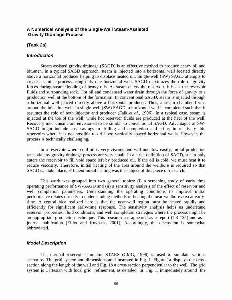
96

A Numerical Analysis of the Single-Well Steam-Assisted Gravity Drainage Process

(Task 2a)

Introduction

Steam assisted gravity drainage (SAGD) is an effective method to produce heavy oil andbitumen. In a typical SAGD approach, steam is injected into a horizontal well located directlyabove a horizontal producer helping to displace heated oil. Single-well (SW) SAGD attempts tocreate a similar process using only one horizontal well. SAGD maximizes the role of gravityforces during steam flooding of heavy oils. As steam enters the reservoir, it heats the reservoirfluids and surrounding rock. Hot oil and condensed water drain through the force of gravity to aproduction well at the bottom of the formation. In conventional SAGD, steam is injected througha horizontal well placed directly above a horizontal producer. Thus, a steam chamber formsaround the injection well. In single-well (SW) SAGD, a horizontal well is completed such that itassumes the role of both injector and producer (Falk et al., 1996). In a typical case, steam isinjected at the toe of the well, while hot reservoir fluids are produced at the heel of the well.Recovery mechanisms are envisioned to be similar to conventional SAGD. Advantages of SW-SAGD might include cost savings in drilling and completion and utility in relatively thinreservoirs where it is not possible to drill two vertically spaced horizontal wells. However, theprocess is technically challenging.

In a reservoir where cold oil is very viscous and will not flow easily, initial productionrates via any gravity drainage process are very small. In a strict definition of SAGD, steam onlyenters the reservoir to fill void space left by produced oil. If the oil is cold, we must heat it toreduce viscosity. Therefore, initial heating of the area around the wellbore is required so thatSAGD can take place. Efficient initial heating was the subject of this piece of research.

This work was grouped into two general topics: (i) a screening study of early timeoperating performance of SW-SAGD and (ii) a sensitivity analysis of the effect of reservoir andwell completion parameters. Understanding the operating conditions to improve initialperformance relates directly to understanding methods of heating the near-wellbore area at early-time. A central idea realized here is that the near-well region must be heated rapidly andefficiently for significant early-time response. The sensitivity analysis helps us understandreservoir properties, fluid conditions, and well completion strategies where the process might bean appropriate production technique. This research has appeared as a report (TR 124) and as ajournal publication (Elliot and Kovscek, 2001). Accordingly, the discussion is somewhatabbreviated.

Model Description

The thermal reservoir simulator STARS (CMG, 1998) is used to simulate variousscenarios. The grid system and dimensions are illustrated in Fig. 1. Figure 1a displays the crosssection along the length of the well and Fig. 1b a cross section perpendicular to the well. The gridsystem is Cartesian with local grid refinement, as detailed in Fig. 1, immediately around the

97

800 m long well. An element of symmetry, with one boundary lying along the wellbore, is usedto represent the reservoir volume. We assume that wells are developed in multiple patterns andthus all boundaries are no flux. The well spacing is 160m. The single horizontal well isrepresented using a discretized wellbore model that accurately represents fluid and heat transferin the well (CMG, 1998). Additionally, the well is broken into two sections to simulate theplacement of a packer. Each section is equal in length and they lie directly end to end. This givesus freedom to explore various completion strategies and operating conditions. Our initialsimulation work suggested that this inject at the toe and produce at the heel strategy had greaterprobability of success than attempting to develop countercurrent steam and oil flow along theentire length of the well.

1,400 mX

Z

800 m Well

19.6 m

InjectionProduction

(a )

(b)Y

Z

19.6 m

80 mWell

Figure 1. Schematic of grid system: (a) parallel to well bore and(b) perpendicular to wellbore.

Initially, the average reservoir pressure is 2,654 kPa (380 psi), the pressure distribution ishydrostatic, and the initial reservoir temperature is 16 °C. The horizontal permeability, kh, is 3400md, whereas the vertical permeability, kv, is 680 md. Hence, the ratio kh:kv is about 5 to 1. The oilviscosity at the initial reservoir temperature is 4.043 Pa-s (4043 cP). An increase of oiltemperature to 100 °C decreases the oil viscosity to 0.030 Pa-s (30 cP). Additional model detailsare documented in Elliot and Kovscek (2001).

Four base cases were created to explore a range of early-time procedures. Briefly thecases represent SAGD operating conditions, extreme pressure differential conditions where steamis injected near the fracturing or parting pressure of the formation, cyclic steam injection, andsteam circulation through the well. For a maximum injection pressure of 10,000 kPa, as reportedin Table 2, the reservoir depth would have to be greater than roughly 450 m to avoid fracturing,

98

assuming that overburden pressure increases at 22.6 kPa/m. Similar maximum pressures havebeen reported in the field (Liderth, 1995). Arbitrarily, 100 d was chosen as the duration ofattempts to heat the near-well region. In all cases, SAGD conditions follow this initial period.


To heat the near-wellbore area and improve the initial production response of SAGD, wecombined the operating conditions displayed in Table 1 into seven cases: (i) SAGD operationconditions from the start, (ii) extreme pressure differential between injector and producer sectionsfor 100 days followed by SAGD, (iii) steam circulation for 100 days followed by SAGD, (iv)circulate for 100 days followed by 100 days of an extreme pressure differential followed bySAGD, (v) cycle once followed by SAGD, (vi) cycle twice followed by SAGD, and (vii) cyclethree times followed by SAGD. In each case except the first, an initial preheating phase precedesSAGD.

Results of this screening study are displayed in Figures 2 to 4. Figures 2 and 3 displayrecovery factor histories for the first year of production and for 10 years of production,respectively. Recovery factor refers to the fraction of oil produced from the entire simulationvolume including the 600 m of reservoir beyond the toe of the well. The cumulative steam oilratio (CSOR) versus time curves for each case are displayed in Fig. 4. It is obvious from thecurves that it is possible to improve initial production response. In general, cyclic steaming asapplied in Cases 5 to 7 leads to the most rapid oil recovery. However, the late time recoveryperformances shown in Fig. 3 display similar behavior for all cases. Recovery factor ranges from19-22% after 3650 days of injection and all curves increase at similar rates.

0.000

0.005

0.010

0.015

0.020

0.025

0 50 100 150 200 250 300 350Time (days)

Rec

over

y Fa

ctor

(fra

ctio

n)

Case 1 - Start at SAGD

Case 2 - Extreme, then SAGD

Case 3 - Circulate, then SAGD

Case 4 - Circulate, then Extreme, then SAGD

Case 5 - Cycle 1X, then SAGD



Case 1

Case 2

Case 3

Case 4

Case 5

Case 6Case 7

Figure 2. Recovery factor for the first year of production.

99

0.00

0.05

0.10

0.15

0.20

0.25

0 500 1000 1500 2000 2500 3000 3500 4000

Tim e (days)

Rec

over

y Fa

ctor

(fra

ctio

n)

C ase 1 - Start at SAG D

C ase 2 - Extrem e, then SAGD

C ase 3 - C irculate, then SAG D

C ase 4 - C irculate, then Extrem e, then SAGD

C ase 5 - C ycle 1X, then SAGD



Case 1

Case 2

Case 3

Case 4

Case 5

Case 6

Case 7

Figure 3. Recovery factor for 10 years of production.

1

10

100

0 500 1000 1500 2000 2500 3000 3500 4000

Tim e (days)

Cum

ulat

ive

Stea

m-O

il R

atio

Case 1 - S ta rt a t SAG DCase 2 - Extrem e, then SAG DCase 3 - C irculate, then SAG DCase 4 - C irculate, then Extrem e, then SAG DCase 5 - Cycle 1X, then SAG DCase 6 - Cycle 2X, then SAG DCase 7 - Cycle 3X, then SAG D

Case 1

C ase 2

C ase 3

Case 5

C ase 4

Case 6

Case 7

Figure 4. Cumulative steam oil ratio for 10 years of production.

Case 1 represents a base case in which SAGD was initiated from the beginning withoutpreheating. This case produced the lowest percent recovery curve. In Case 2, we increase theinjection rate constraint which thereby increases the pressure differential between the injectionand production wells; hence, the conditions are referred to as extreme. The pressurization of thesystem improves production somewhat relative to the base case.

The “circulate” phase in Cases 3 and 4 is a modified form of steam circulation in the well.Steam is injected so as to maintain the initial reservoir pressure. We did not simulate true steamcirculation where steam that exits the tubing may only flow in the well before it is produced. Atrue circulating case in which the near-wellbore area is heated only by conduction would beinefficient, and the other techniques that we explore present better options. Circulation here issimilar to the SAGD case: steam may replace oil volume in the reservoir when oil is produced.

100

The cumulative steam oil ratio displayed in Fig. 4 is standard: the cumulative steamvolume injected as cold water equivalent volume divided by the cumulative hydrocarbonproduction. The CSOR varies substantially among the studies during the initial period becausesignificantly different production and injection schemes were used. At late time, however, theCSOR for all cases averages roughly 3.0. Note, however, that the cyclic cases perform somewhatbetter, with regard to CSOR, in initial and late-time response.

Discussion of Early-Time Analysis

The problem of improving early-time performance of SW-SAGD transforms, essentially,into a problem of heating rapidly the near-wellbore area to create conditions that allow gravitydrainage of oil. More specifically, for a steam chamber to grow, oil viscosity must be low enoughso that fluid drains creating voidage for steam to fill. After the conditions necessary for gravitydrainage of oil have been initiated by preheating, the SW-SAGD process allows for continuoussteam chamber growth and oil production. Comparing the various simulation results, cyclic steaminjection appears to be the most efficient method of heating the near-wellbore area. Heating ismuch more rapid than relying on conduction alone.

An important general observation is that regardless of the process, early-time proceduresshould be carried out to maximize steam injection and heat delivery to the reservoir. The goal ofany early-time procedure should be to heat the near-wellbore area as uniformly as possible. Thisgoal is easier to achieve when operating at a maximum steam temperature. Later in the SAGDprocess, pressure can and should be reduced to a target operating pressure that optimizesefficiency and production rate.

The late time performance for all of the cases is favorable regardless of the early-timeprocess. This confirms Joshi’s finding that a steam chamber will grow in the reservoir. Favorablerecovery factors are obtainable regardless of the injection/ production configuration (Joshi, 1986).

There are obvious factors that will improve or inhibit SW-SAGD performance. Forexample, lower viscosity will certainly improve response, as will larger rock permeability andsystem compressibility. The actual variance in performance due to differing reservoir parametersis an interesting problem that we begin to address using a sensitivity analysis in the next section.

Sensitivity Analysis

We performed a sensitivity analysis of various reservoir parameters to gain a betterunderstanding of their effect on production performance. Oil viscosity and gas content, reservoirthickness, and horizontal to vertical permeability anisotropy were studied.

The sensitivity analysis base case varies slightly from the base case used in the early-timeanalysis. Table 2 displays the operating conditions for the sensitivity analysis base case. The basecase consists of two steam injection cycles followed by SAGD operating conditions. We adjustedthe operating conditions in an attempt to reduce steam short-circuiting, reduce steam-oil ratio, and

101

to improve efficiency. During the initial cyclic period, we reduced the maximum reservoirpressure to 8,000 kPa from 10,000 kPa while keeping the rest of the operating conditions thesame. The steam injection temperature was 296 °C, that corresponds to a steam pressure of 8004kPa. During SAGD, operating conditions were chosen so that the process operated near theoriginal reservoir pressure of 2654 kPa. Maximum injection pressure was set slightly aboveinitial reservoir pressure at 3230 kPa; minimum production pressure was set slightly below initialreservoir pressure at 2230 kPa. The steam injection temperature was reduced to 238 °C from 295°C. Initial reservoir conditions were chosen to approximate field conditions (Oballa andBuchanan 1996). The rate constraints remained the same at 300 m3/d maximum liquid productionand 200 m3/d maximum steam injection rate.

Table 1. Grid, Rock, and Oil Property Description.

Grid System Rock Propertiestotal no. blocks

5,568 porosity 33%

x-dimension 1,400 m kh 3,400 mDy-dimension 80 m kv 800 mDz-dimension 19.6 mwell length 800 m

Reservoir Properties Oil Propertiesinitial pressure 2,654 kPa components water, oil, and gasinitialtemperature

16 °C initialcomposition

90 % (mole) oil

initial So 85% 10% (mole) gasinitial Sw 15% viscosity

(mPa-s) versustemperature (K)function

µ = 1 . 74x 10− 6 exp 6232 . 74T

Between the injection and production sections of the horizontal well, a 30 m longunperforated section was added. This is an attempt to force steam to penetrate substantially farinto the reservoir and reduce the amount of steam short-circuiting.

102

Table 2: Operating Conditions for Early-Time Performance Study

Property Operating ConditionSAGD Extreme Cyclic Circulating

steamtemperature(°C)

295 295 295 295

max. injectionrate (CWEm3/day)

200 600 300 300

max. injectionpressure (kPa)

10,000 10,000 10,000 10,000

max.productionrate (m3/day)

300 600 300 300

min. productionpressure (kPa)

500 500 500 500

Sensitivity Cases

The various cases created in the sensitivity analysis include: (i) a base case with theproperties in Table 1 and operating conditions shown in Table 3, (ii) dead oil to examine theeffect of solution gas, (iii) an increase in pay thickness to 28 m, (iv) a reduction in pay thickess to4 m, (v) permeability anisotropy kh:kv of 1, (vi) kh:kv equal to 2, (vii) kh:kv equal to 10, (viii) oilviscosity of 20 Pa-s at initial reservoir temperature (20,000 cP), and (iv) oil viscosity of 40 Pa-s(40,000 cP) at initial reservoir temperature.

All calculations in the sensitivity cases include a separation of 30 m between injector andproducer sections of the well to achieve better steam distribution in the reservoir. Two periods ofcyclic steam injection precede continuous injection and production. In both periods, steam isinjected for 50 days at a rate of 300 m3/day with a maximum allowed pressure of 8000 kPa. Thesoak period is 10 days and the length of production is a relatively short 40 days to avoid largeheat withdrawal from the reservoir. Continuous SAGD operating conditions follow. All of thevarious sensitivity runs follow this procedure.

The recovery factor versus time and cumulative steam-oil ratio (CSOR) versus timecurves are presented in Figs. 5 and 6, respectively. Again, recovery refers to the entire simulationvolume. Significant variation is found in production response between most of the cases. Briefly,production is greatest when the reservoir permeability is isotropic, and is worst when the initialoil viscosity is high or the oil-saturated thickness is small. The steam-oil ratio is largest for theshort formation thickness of 4 m. The next largest CSOR is for the viscous 40 Pa-s initial oil case.The smallest CSOR is found for the case with a pay zone thickness of 28 m and for cases wherekh:kv approaches 1. Note that recovery factors are less here, Fig. 5, compared to the early-timestudy, Fig. 3, because the steam injection pressure has been reduced substantially as seen bycomparing Tables 1 and 2.

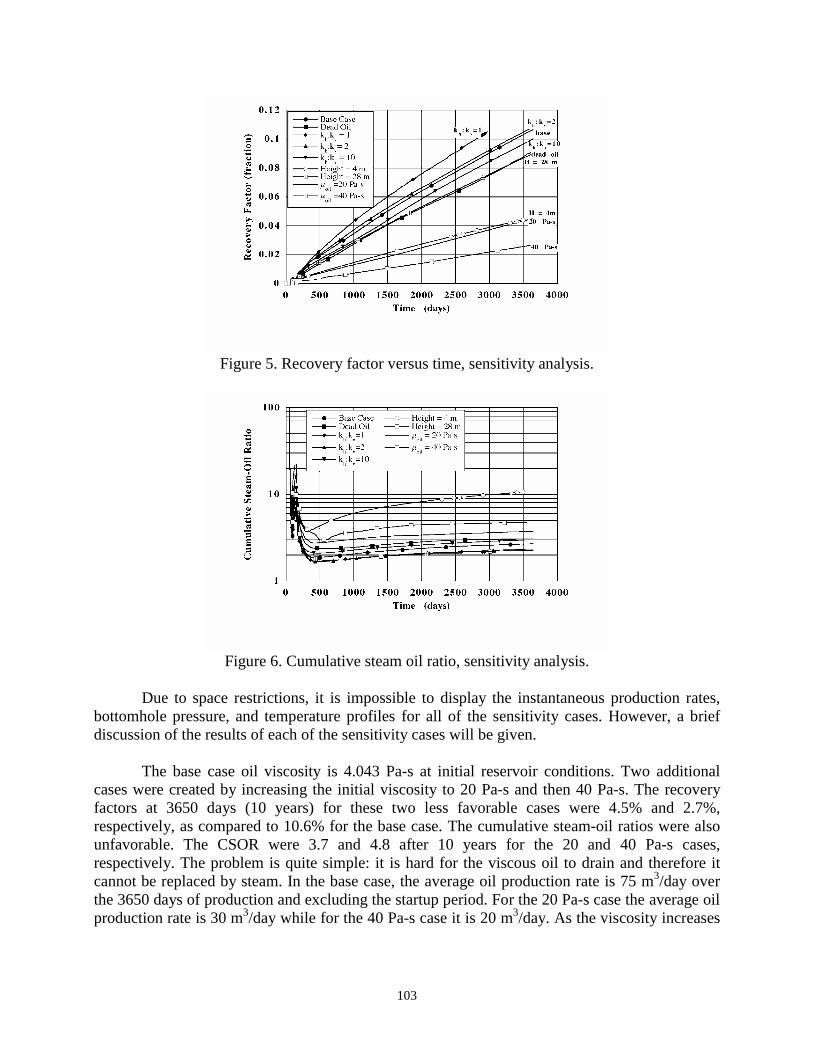
103

Figure 5. Recovery factor versus time, sensitivity analysis.

Figure 6. Cumulative steam oil ratio, sensitivity analysis.

Due to space restrictions, it is impossible to display the instantaneous production rates,bottomhole pressure, and temperature profiles for all of the sensitivity cases. However, a briefdiscussion of the results of each of the sensitivity cases will be given.

The base case oil viscosity is 4.043 Pa-s at initial reservoir conditions. Two additionalcases were created by increasing the initial viscosity to 20 Pa-s and then 40 Pa-s. The recoveryfactors at 3650 days (10 years) for these two less favorable cases were 4.5% and 2.7%,respectively, as compared to 10.6% for the base case. The cumulative steam-oil ratios were alsounfavorable. The CSOR were 3.7 and 4.8 after 10 years for the 20 and 40 Pa-s cases,respectively. The problem is quite simple: it is hard for the viscous oil to drain and therefore itcannot be replaced by steam. In the base case, the average oil production rate is 75 m3/day overthe 3650 days of production and excluding the startup period. For the 20 Pa-s case the average oilproduction rate is 30 m3/day while for the 40 Pa-s case it is 20 m3/day. As the viscosity increases

104

the average oil production rate decreases, it becomes difficult to meet the steam injection target,and the size of the steam chamber is smaller compared to the less viscous cases.

The base horizontal to vertical permeability ratio, kh:kv, is 4.25. The vertical permeabilitywas adjusted to create three more cases with ratios of 1, 2, and 10. In all cases, the horizontalpermeability remained fixed at 3400 mD. Larger ratios present less favorable conditions forupward steam migration and oil drainage. As kh:kv increases, cumulative recovery at a given timedecreases and the CSOR increases, as shown in Figs. 5 and 6.

The base case oil composition contained 10% gas by mole which translates to a solutiongas oil ratio of about 28 SCF/STB. An additional case that models a dead oil was created byreducing the solution gas to 1% by mole. The two effects of solution gas in regard to the oil phaseare to increase oil-phase compressibility and reduce the oil-phase viscosity. Oil phase viscosity iscomputed as a mole fraction weighted sum of the oil and gas component viscosities (CMG 1998).Recovery factor and CSOR were less favorable with the dead oil at 9.2 % and 3.0 after 10 yearsas compared to 10.4% and 2.8 for the base case. Likewise, the average oil production rate is 64m3/day over the ten year period as compared to 80 m3/day for the base case.

Discussion of Sensitivity Analysis

Taken together, the results from the sensitivity analysis suggest that application of SW-SAGD to exceptionally viscous oils will be difficult. When the initial viscosity is greater than 10Pa-s, oil drainage becomes very slow and it is difficult to form a large steam chamber. Likewise,the application of SW-SAGD to thin oil zones with thickness of roughly 4 m does not appear tobe feasible. A steam chamber of significant height must develop for efficient oil drainage. Onthe other hand, the 19.6 and 28 m thick cases showed significant recovery and little differencewas found between theses two cases.

The presence of solution gas also aids recovery somewhat. Even though the oil is viscousand the amount of gas low in both cases, volumetric expansion of the oil is aided by solution gasand cumulative recovery increases by 10% relative to the dead oil case at 3650 days.

As expected, oil recovery improves as the permeability anisotropy decreases. Both steaminjection and oil drainage are aided as the vertical permeability increases relative to thehorizontal. Resistance to flow in the vertical direction decreases relative to horizontal.Additionally, less short circuiting occurs as kv increases relative to kh.

Conclusions

Here it is shown that to improve early-time performance of SW-SAGD, it is necessary toheat the near-wellbore region rapidly and uniformly to reduce oil viscosity and promote gravitydrainage. Cyclic steaming, as a predecessor to SW-SAGD, represents the most thermally efficient

105

early-time heating method. Uniform heating along the length of the wellbore appears achievablewith cyclic steam injection. Immediately placing a cold well on SAGD hinders the early-timeheating process and initial production response in this case will be low. Regardless of the early-time process, it should be performed to provide maximum heat delivery to the reservoir.Additionally, despite different initial procedures, the oil production rates after several years ofsteam injection are all very similar.

The sensitivity analysis performed here indicates that SW-SAGD is most applicable toheavy oils with initial viscosity below 10 Pa-s (10,000 cP) Additionally, the reservoir must besufficiently thick to allow significant vertical steam chamber growth. Recovery from thin oilzones is not significant or efficient. The sensitivity analysis also indicates that the presence ofrelatively small amounts of solution gas aids the recovery process by enhancing volumetricexpansion of the oil on heating.

References

Computer Modelling Group LTD. 1998. STARS Version 98 User's Guide. CMG Calgary,Alberta, Canada.

Elliot, K. T. and A. R, Kovscek, “A Numerical Analysis of the Single-Well Steam AssistedGravity Drainage Process,” Petroleum Science and Technology, 19 (7 and 8), 733-760,2001; also TR 124, DOE DE-FC26-00BC1531, 2001.

Falk, K., Nzekwu, B., Karpuk, B., and Pelensky, P. 1996 World Oil. July: 85-95.

Liderth, D. 1995. Daily Oil Bulletin, May 2, 1995.

106

Analytical Model for Cyclic Steam Stimulation of a Horizontal Well

(Task 2a)

Introduction

The previous section illustrated that cyclic steaming as a precursor to steam-assistedgravity drainage may be an effective means of stimulating a heavy-oil formation therebyproducing oil at appreciable rates relatively quickly. This work concerns the application ofhorizontal wells to thermal oil recovery. It consists of an analytical model developed to calculateoil recovery and reservoir heating during cyclic steam injection. It holds for heavy-oil, pressure-depleted reservoirs where the main driving force for production is gravity. Our objective is topresent a relatively simple model taking into account gravity-drainage along the sides of the steam-oil interface, the pressure draw down driving force and the drainage of oil through the steam zone.

The performance of horizontal wells may be predicted from empirical correlations, simpleanalytical models, or thermal reservoir simulation. Empirical correlations can be extremely usefulfor correlating data within a field and for predicting performance of new wells in that and similarfields. However, use of such correlations for situations much different from those that led to theirdevelopment might be subject to large errors. On the other hand, one can use a compositional orblack-oil thermal model to predict the performance of cyclic steam operations. Thermal models arebased on the fundamental laws of conservation of mass and heat. Fluid flow is related to pressuregradient through the concept of relative permeability. In addition, a thermal model is sensitive torock properties, fluid properties and geological features. Much of this information is oftenunknown and must be estimated from limited data and experience in similar situations.Furthermore, because of the complexity of the SAGD recovery process, the equations of a thermalsimulator could be difficult and expensive to solve depending upon the exact scenario. Simply, ananalytical model of cyclic steam injection is useful to expose the first-order mechanisms ofreservoir heating and oil production.

Model Development

Cyclic steam injection, commonly referred to as "Huff-n-Puff" involves steam injectioninto a reservoir, followed by soaking, and finally the oil production period. As stated earlier, oilproduction is governed by the gravity driving force. The model developed in the following sectionincorporates gravity as a prime driving force for oil flow towards the well and thereby predicts theoil production flow rate per unit length of the horizontal well in the production period. Heat lossesfrom the heated zone to the overburden and the adjacent unheated oil-bearing formation are alsoincluded.

By way of background, steam introduced at the bottom of the formation through ahorizontal well, displaces the oil and rises to the top of the formation where it is trapped if animpermeable cap rock exists. We assume that the steam zone adopts a triangular shape in cross

107

section as shown in Fig.1. The steam injection rate around the well remains constant over theentire injection interval. Therefore, the steam injection pressure generally remains constant overthe injection process if the reservoir is pressure-depleted. Steam heats up the colder oil sand nearthe condensation surface and oil drains along the condensation surface by a combination of gravityand pressure difference into the production well. Steam condensate also drains toward the well. Inaddition, oil drains through the steam chamber into the production well. The mechanisms involvedin oil production during cyclic steam injection are diverse and intricate. Reduction of oil viscosityas a result of an increase in the temperature greatly improves the production response. Gravity-drainage and pressure drawdown are the major mechanisms of oil production in the case of cyclicsteaming.

x qo

rhst

dθ dθ

θ

(a) (b)

Figure 1. (a) Schematic of heated area geometry; (b) differential element of the heated area.

The model is divided into three periods: the injection period, the soaking period and theproduction period. Each is described in detail. In what follows, correlations and equations aregiven in field units (°F, psi, ft, BTU, BPD, etc), unless otherwise noted.

Injection and Soak Periods

During the injection interval, heat losses from the steam zone to the reservoir areconsidered negligible although heat losses to the overburden must be considered. The oil sand nearthe wellbore is assumed to be at steam temperature Ts, the saturated steam temperature at the sandface injection pressure. Pressure fall-off away from the well during injection is neglected duringthis analysis. In the soaking period, heat is lost to the overburden and the reservoir. Thetemperature of the steam zone thus decreases while soaking.

There are certain important variables such as the steam zone volume and the zonehorizontal range that need to be addressed. The steam zone volume, Vs, during injection iscalculated using the approach of Myhill and Stegemeier (1978) as

Vs =QiEh,s

MT∆T(1)

108

where, Eh,s is the thermal efficiency, ∆T is the temperature rise of the steam zone above the initialreservoir temperature (assumed to be same as the temperature rise at down-hole condition, ∆Ti),and MT is the total volumetric heat capacity of the reservoir. Heat capacity is the sum of the rockand fluid contributions and is written

MT = 1 − φ( )Mrr + φSβMββ=w,o,g∑ (2)

where, φ is the porosity, S is the phase saturation, and the subscript β refers to the individualphases. The quantity Qi is the cumulative heat injected including any remaining heat from theprevious cycles. The heat injection rate is given by

( )vdhsdhwii HfTCwQ ∆+∆= (3)

where, wi is the mass rate of steam injection in the reservoir, Cw is the average specific heat ofwater over the temperature range corresponding to ∆T, fsdh and ∆Hvdh are the steam quality and thelatent heat of vaporization both at down-hole conditions, respectively.

The thermal efficiency is calculated from the function given by Myhill and Stegemeier(1978) as

Eh,s =1

tDG tD( )+ 1 − fhv( )U tD − tcD( )

π2 tD − 2 1− fhv( ) tD − tcD −

exerfc x( )tD − x

dx − πG tD( )0

tcD∫

(4a)

In the expression above, the heat losses to both, the overburden as well as the underburden areincluded. In the model proposed, the triangular cross sectional shape of the steam chamber is suchthat heat loss occurs only to the overburden. Thus, Eh,s needs to be modified to be consistent withour model. Now, Eh,s is defined as the ratio of the heat remaining in the zone to the total heatinjected. Thus, the quantity (1-Eh,s) is the ratio of the heat lost to the total heat injected

Fl = 1-Eh,s (4b)

Neglecting loss to the underburden, heat losses are approximately one-half of the value predictedby Eq. 4b. Therefore, the modified thermal efficiency is

(Eh,s)mod = 1- 0.5 Fl = 0.5 (1.0 + Eh,s) (4c)In Eq. 4a, G(tD) is

( ) ( )DtD

D terfcettG D+−= 12π

(5)

The symbols tD and tcD represent dimensionless times given by

tD = 4MSHMT

2α SHht

2 t (6)

109

where, αSH is the shale thermal diffusivity, t is the time, ht is the total reservoir thickness and MSHis the shale volumetric heat capacity. The dimensionless critical time (Myhill and Stegemeier,1978) is defined by

etcD erfc tcD( )≡ 1− fhv (7)

The quantity fhv, the fraction of heat injected in latent form, is given by

fhv = 1 +Cw∆T

fsdh∆Hvdh

−1

(8)

The step-function U in Eq.4 is defined as

U x( ) = 0 for x < 0 (9a)

U x( ) = 1 for x > 0 (9b)

We assume that the steam zone shape has a triangular cross section with a y-directional lengthequal to the length of the horizontal well, L (Fig.1). The volume is written as

Vs = RhLhst (10a)

where Rh is one-half of the base of the triangular heated zone and hst is the steam zone thicknessalso referred to as "Zone Horizontal Range". Rearranging Eq.10a, it follows that,

Rh =Vs

Lhst(10b)

Heat Remaining in the Reservoir

Boberg and Lantz (1966) give the average temperature of the steam zone, Tavg, as

Tavg = TR + Ts − TR( ) fHD fVD 1 − fPD( )− fPD[ ] (11)

The dimensionless parameters fVD, fHD and fPD are functions of time and represent horizontal loss,vertical loss and energy removed with the produced fluids, respectively. Aziz and Gontijo (1984)define them according to the following expressions.

The horizontal heat losses are expressed as (Aziz and Gontijo, 1984):

DHHD t

f511

+= (12a)

110

where,

tDH =α t − tinj( )

Rh2 (12b)

The quantity fHD is the average unit solution for the one-dimensional heat conduction problem inthe horizontal direction,

α∂2 f∂x2 =

∂f∂t

(12c)

where f =T − ToTs − To

is the dimensionless temperature and α is the reservoir thermal diffusivity.

The averaged solution for this equation after making use of the appropriate boundaryconditions consistent with the geometry chosen for our model is:

fHD =12

+tDHπ

−2.0 + exp −1

tDH

+ erf

1tDH

2π

−1

tDH +

12

(12d)

Similarly, the vertical heat losses are expressed as (Aziz and Gontijo, 1984):

fVD =1

1 + 5tDV(13a)

where,

tDV =4α t − tinj( )

ht2 (13b)

Note that for the first cycle, the initial amount of heat in the reservoir is set to zero. For allfollowing cycles, the initial amount of energy is calculated based on steam zone volume and theaverage temperature at the end of the previous cycle. The average temperature at any time duringthe cycle is calculated using Eq.11 (Boberg and Lantz, 1966). Since Boberg and Lantz’s equationassumes a cylindrical shape for the heated zone, this equation is just an approximation for thetriangular shape being considered. However, we use the approximations for fHD and fVD asemployed by Aziz and Gontijo (1984) who assume a conical shape with triangular cross section.This is identical to the cross sectional shape that we have considered. The only difference is thatthey rotate the triangular shape through π radians whereas our coordinate system is Cartesian.

The term that accounts for the energy removed with produced fluids is given by

fPD =1

2QMAXQpdt

0

t∫ (14)

where, Qp = 5.615 qoMo + qwMw( ) Tavg − TR( ) (15)

111

where QMAX is the maximum heat supplied to the reservoir. It is calculated at the end of the soakperiod as the amount of heat injected plus the heat remaining in the reservoir from the previouscycle minus the losses to the over burden (Vogel, 1982),

QMAX = Qinj + Qlast − 2Rh LKR Ts − TR( ) tsoakΠα

(16a)

Qinj = 350.376Q iwstinj (16b)

Qlast = VsMT (Tavg − TR) (16c)

where, L is the length of the horizontal well, KR is the thermal conductivity of thereservoir, tsoak is the soak time, tinj is the length of the injection cycle, Qlast is the heat remainingfrom the previous cycle, Q i is the amount of heat injected per unit mass of steam, and ws is thesteam injection rate (cold water equivalent).

The steam pressure is calculated from the following approximate relationship (Prats,1982):

ps =Ts

115.95

4.4545(17)

The volumetric heat capacities of oil and water are given as (Prats, 1982):

Mo = 3.065 + 0.00355T( ) ρo

Mw = ρwCw(18)

As the integral for fPD is not easy to calculate, it is approximated by the following expression (Azizand Gontijo, 1984),

∆fPD =5.615 qoMo + qwMw( ) Tavg

n−1 − TR( )∆t2QMAX

(19)

where, ∆t is the time step, n is the time step number, qo and qw are the oil and water productionrates, respectively. The average temperature of the steam zone in the ‘n-1’th cycle is 1−n

avgT .

Production Period

In this period, the well is opened for oil flow from the reservoir. A new model is presentedto predict oil production rates during the production period. Butler et al. (1980) presented a seriesof publications related to the gravity-drainage of heavy-oil reservoirs subjected to steam injectionin which the theory was directed to linear flow from horizontal wells. In this development, asimilar approach is used. However, the steam zone shape has been assumed to be a prism with

112

triangular cross section and the horizontal well lies at the bottom edge. Figure 1 shows the crosssectional shape of the zone.

It is assumed in the derivation of the flow equation that the reservoir is initially saturatedwith oil and water, and it is pressure-depleted. After steam flooding, the steam chamber occupies aprismatic shape. Steam distribution along the well is assumed to be uniform. Heat transfer fromthe steam chamber to the neighboring oil zone is via conduction. During the injection period, theaverage temperature of the steam chamber is assumed to be the saturation temperature of thesteam. The oil is heavy enough to permit the injected steam to go to the top of the reservoir assuggested by Van Lookeren (1977). The reservoir is assumed to be initially pressure-depleted andis only negligibly re-pressurized when steam is injected. Finally, the potential that causes flow ofoil into the same well that acts as a production well is a combination of gravity forces and pressuredrive.

In this approach, we assume that gravity-drainage takes place through the entire steamchamber. Thus, integration is over the entire steam chamber and proceeds angularly with theappropriate approximation for the area. Gravity and pressure drive are taken as the forces causingproduction. The steam zone growth is estimated in terms of the decrease in the angle of inclinationof the zone with the horizontal, q. The thickness of the steam zone is assumed to be equal to thereservoir thickness. The heated-zone geometry used to derive the flow equation is given in Fig.1.The maximum heated dimension in the horizontal direction is Rh, while the maximum heateddimension in the vertical direction is the reservoir thickness h.

According to Darcy’s law, the flow rate through an incremental area, dA, normal to thedirection of flow [Fig.1(b)], is written

dqo = −koµo

ρo − ρs( )∇φ dA (20a)

where, ∇φ is the gradient of potential in the direction of flow, µo is the dynamic viscosity of oil, kois the effective permeability to oil, and ρo - ρs is the density difference between the oil and steam.According to Hubbert (1956 ), the potential is expressed as

hgpp

o

wfs ∆+−

=∆ θρ

φ sin (20b)

Here, g is the acceleration due to gravity. The differential area depends upon distance, r, above thewell:

dA = 2r sin12

dθ

≈ rdθ (21)

The oil-phase effective permeability, ko is the product of the absolute permeability, k, and relativepermeability, kro. With r equal to hstcosec(θ) and applying the approximation suggested in Eq.21,the differential area reduces to

dA = Lhst cosecθdθ (22)

113

It follows upon substitution of Eq.22 into Eq.20 that the flow rate becomes

dqo = −koµo

ρo − ρs( ) ps − pwf

ρo+ ghst sin θ( )

hst Lcosecθdθ (23)

Integration over one-half of the heated area and multiplication by 2 yields

qoL

= −2koµo

ρo − ρs( ) 144.0ps − pwf

ρolog

1

tanθ2

+ ghst π −2θ( )

(24)

Property Correlations

A variety of property correlations are needed as constitutive relations. The steam viscosityand density are calculated by correlations given by Farouq Ali (1982). The average specific heat ofwater is obtained as

Cw =hw Ts( )− hw TR( )

Ts − TR(25)

The water enthalpy correlation of Jones (1977) and the steam latent heat correlation of Farouq Ali(1982) are used to obtain water properties. The oil and water densities are approximated byaccording to the information given by Aziz (1984). These oil density correlations hold for oils withgravity less than 20oAPI and temperature less than 500oF.

Fluid viscosities as a function of temperature are obtained from relations given by Jones(1977). This correlation for oil viscosity is applicable to oils with specific gravity less than 30o

API.

After the soak period and before the production begins, it is assumed that the only mobilephase around the well is water

S w = 1− Sorw (26)

Once the well is opened for production, it is assumed that the oil saturation around the wellincreases. Also, the water saturation is given by

Sw = S w − S w − Swi( ) Wp

WIP(27)

where Wp is the water production during the cycle and WIP is the amount of mobile water in placeat the beginning of the cycle (Aziz and Gontijo, 1984). The normalized water saturation expressionis

Swo =

Sw − Swi1− Swi − Sorw

(28)

114

The analytical expressions presented by Farouq Ali (1982) for the relative permeabilitiessuggested by Gomaa (1980) are as follows:

krw = −0.002167Swo + 0.024167 Sw

o( )2 (34a)

kro = −0.9416 +1.0808

Swo −

0.13856

Swo( )2

(34b)

with,

kro = 1.0 if Swo ≤ 0.2 (34c)

Algorithm for Calculation Scheme

These equations and ideas are translated into a seven-step algorithm:• Initialize the model by inputting reservoir, fluid, and operational properties.• Calculate steam zone geometry (volume, height, and thickness), temperature, and

saturations during injection and at the start of the production cycle.• Calculate oil and water production flow rates at small time steps within the production

interval. Also, calculate the cumulative volume of fluids produced and check againstoriginal fluids in place.

• Calculate the average temperature of the heated zone during production and at the end ofthe production cycle.

• If additional steps are needed for cycle completion, go to stage 3, else proceed.• Calculate the amount of fluids and heat remaining in the reservoir at the termination of the

cycle, and thereby calculate recovery and oil-steam ratio (OSR).• If a new cycle is required, repeat steps, else terminate calculations.


Similar reservoir and fluid models were assembled for comparison of the semi-analyticalcalculation versus thermal reservoir simulation using CMG STARS. Input parameters aresummarized in Table 1. A two-dimensional homogeneous permeability field was constructed forsimulation. There are 55 by 13 gridblocks in the horizontal and vertical directions, respectively.The grid is refined locally near the well. The horizontal direction is sufficiently large (7,495 ft.) soas to represent a semi-infinite system in lateral extent. Injection and soak periods are set to 45 and20 days, respectively. Three huff-n-puff periods are calculated and the elapsed production periodincreased for each subsequent cycle. The production periods are chosen as 50, 100, and 140 for thefirst, second, and third cycles.

Figure 2 illustrates the match between cumulative oil production from semi-analyticaltheory and reservoir simulation. Results for the first cycle match well. For the second and thirdcycle, the semi-analytical theory over predicts the cumulative oil production significantly. That is,the oil production rate from the semi-analytical theory is somewhat larger than that predicted bythe reservoir simulator.

115

Table 1. Physical Properties for Semi-Analytic Calculation and Simulation

Variable Valuepermeability (Darcy) 1.5porosity 0.2initial water saturation 0.25connate water saturation 0.10well radius (ft) 0.31residual oil saturation to steam 0.05residual oil saturation to water 0.25initial reservoir temperature (°F) 110saturated steam temperature (°F) 365thermal conductivity (BTU/ft-D-°F) 24.0thermal diffusivity (ft2/day) 0.48time step (day) 1.0injected steam quality 0.67steam injection rate (bbl/d/ft of well) 1.0API gravity of oil 14.0injection pressure (psi) 150.0pay thickness (ft) 80.0

After substantial investigation, it has been found that the temperature of the steam zone ascomputed by both methods differed somewhat. Figure 3 presents the temperature of the steamzone versus time that complements the cumulative oil production in Fig. 2. The upper curverepresents the temperature history as predicted by the semianalytical model and it well illustratemodel assumptions. That is, temperature is constant during the injection period, relatively slowdecline in temperature during soak, and then a somewhat greater decline in temperature during theproduction period. The greater decline in temperature during production signifies the production ofhot reservoir fluids. The temperature history as predicted by the reservoir simulator has many ofthe same features as that from the semi-analytical theory. The primary difference between the twocurves is the temperature reached during injection. The semi-analytical theory predicts a steamtemperature of roughly 365 °F commensurate with the injection bottom hole pressure of 150 psiwhereas the reservoir simulator has a temperature during injection of about 240 °F. Thetemperature is lower in the simulation and thus the oil viscosity is greater as compared to the semi-analytical theory. Because the oil viscosity is greater in the simulation, oil drains more slowlyreducing the cumulative oil production as compared to the semi-analytical theory. No reason forthe discrepancy in temperature is apparent.

116

0

50

100

150

200

250

300

350

400

450

500

0 100 200 300 400 500 600

time(day)

Cum

ulat

ive

Oil

Prod

uctio

n(bb

l)

semi-analytical modelSTARS

Figure 2. Comparison of semi-analytic model and reservoir simulation results.

Despite the lack of qualitative agreement, the semi-analytical theory is useful to display therelative sensitivity of various reservoir parameters. Figure 4 illustrates the effect of increasing theinjection period to 100 days to increase the amount of energy input to the system. Again, threecycles are simulated. Figure 4 also shows the result obtained with 45 days of injection, as above.The additional heat benefits production in all cycles and, for instance, increases the cumulative oilrecovered in the second cycle by almost 50%.

On the other hand, the semi-analytical model is also helpful to illustrate parameters thathave little influence on the results expected. Figure 5 summarizes the results from examining thesensitivity of production to heat losses to the overburden by adjusting the thermal conductivity ofthe overburden. Both semi-analytical and reservoir simulation results are given. Both display thesame qualitative behavior and illustrate that decreasing the heat losses by one half changes thecumulative production very little. Thus, heat losses to the overburden are relatively unimportantduring the initial stages of cyclic steaming. Most of the heat injected remains in the productiveinterval enhancing production.

117

0

50

100

150

200

250

300

350

400

0 100 200 300 400 500 600

time(day)

aver

age

tem

pera

ture

(°F)

semi-analytical theorySTARS

Figure 3. Comparison of steam zone temperature

118

0

100

200

300

400

500

600

700

800

900

0 100 200 300 400 500 600 700

time

Cum

ulat

ive

Oil

Prod

uctio

n (b

bl)

semi-analytical theory, 45 day injection period

semi-analytical theory, 100 day injection period

STARS, 45 day injection period

STARS, 100 day injection period

Figure 4. Sensitivity of cumulative oil production to the duration of injection.

119

0

100

200

300

400

500

600

700

800

900

0 100 200 300 400 500 600 700

time

Cum

ulat

ive

Oil

Prod

uctio

n (b

bl)

semi-analytical theory, 1/2 heat lossessemi-analytical theorySTARS, 1/2 heat lossSTARSsemi-analytical theory, 45 day injection periodsemi-analytical theory, 100 day injection periodSTARS, 45 day injection periodSTARS, 100 day injection period

Figure 5. Sensitivity of cumulative oil production to heat losses.

Conclusions

A simple model has been developed for the cyclic steam process with a horizontal well. Itincorporates a new flow equation for gravity drainage of heavy oil. Important factors such aspressure drive, gravity drive, and shape of the steam zone are incorporated into the model.Limited comparisons of the model to numerical simulation results indicate that the modelcaptures qualitatively the essential physics of the recovery process. Nevertheless, the lack ofquantitative agreement suggests that further research is needed to refine the model and complete afull verification exercise.

Generally, cyclic steaming appears to be effective in heating the near well area and thereservoir volume surrounding a horizontal well. A sensitivity analysis shows that the process isrelatively robust over the range of expected physical parameters. As such, cyclic steaming is an

120

effective process to warm cold reservoirs containing viscous oil prior to continuous steaminjection processes such as steam-assisted gravity drainage.

References

Aziz, K. and Gontijo J.E.: "A Simple Analytical Model for Simulating Heavy-oil Recovery byCyclic Steam in Pressure-Depleted Reservoirs", paper SPE 13037 presented at the 59thAnnual Technical Conference and Exhibition, Houston, September 16-19, 1984.

Boberg, T.C. and Lantz, R.B.: “Calculation of the Production Rate of a Thermally StimulatedWell”, J.Pet.Tech. (Dec. 1966).

Farouq Ali, S.M.: "Steam Injection Theories – A Unified Approach", paper SPE 10746 presentedat the California Regional Meeting of the SPE, San Francisco, March 24-26, 1982.

Jones, J.: "Cyclic steam Reservoir Model for Viscous Oil, Pressure-depleted, Gravity-drainageReservoirs", SPE 6544, 47th annual California Regional Meeting of the SPE of AIME,Bakersfield, April 13-15, 1977.

Myhill, N.A. and Stegemeier, G.L.: “Steam Drive Correlation and Prediction”, J. Pet. Tech. (Feb.1978) 173-182.

Prats, M.: "Thermal Recovery", Monograph – Volume 7, SPE of AIME, Henry L. DohertyMemorial Fund of AIME, 1982.

Van Lookeren: “Calculation Methods for Linear and Radial Steam Flow in Oil Reservoirs”,J.Pet.Tech. (June, 1983) 427-439.

Vogel, V.: "Simplified Heat Calculation of Steamfloods", paper SPE 11219 presented at the 57thSPE Annual Fall Technical Conference and Exhibition, New Orleans, LA, September 26-29, 1982.

121

Efficiency and Oil Recovery Mechanism of Steam Injection into Low Permeability,Hydraulically Fractured Reservoirs

(Task 2b)

Introduction

Low-permeability fractured reservoirs contain a large volume of the worldwide oilresource (Saidi, 1983), yet production from these reservoirs has been modest. Primaryproduction is low, usually 5% - 10% of the original oil-in-place. Furthermore, waterfloodscommonly suffer from low injectivity, poor sweep, and injector-to-producer linkage. Thesefactors tend to degrade waterflood’s effectiveness and have facilitated an attempt to use enhancedrecovery techniques. At Teapot Dome Field in central Wyoming steam was injected into in alow-permeability fractured reservoir containing a light oil (32º API) (Olsen et al., 1992; Olsen etal., 1993; Doll et al., 1995). While this reservoir did not perform up to initial expectations, itshowed that steam injection was feasible. Also, the importance of steam quality and the need fora sizeable Soφ (the volume of oil per unit rock volume) was more clearly understood. Additionalexamples include fractured carbonates such as Ghaba North in Oman (27º API). A study is underway to determine if steam can increase production economically in such fields (cf. Al-Hadhramiand Blunt, 2001). Also, a pilot in the Yates Field of west Texas (30º API) has initiated and isshowing promising results (Moritis, 2002).

The South Belridge field (California) has undergone a number of steam injection pilottests into low permeability (0.1 md) fractured reservoir containing light oil. Initial results fromtwo of these pilots have demonstrated that these reservoirs respond very well to steam injection(Johnston and Shahin, 1995; Kovscek et al., 1996 I, II). A larger field project is underway atSouth Belridge but, as of yet, no data are reported. For these reasons, and because a significantamount of information about diatomite was made available to us, this study uses diatomite as itsbasis. Nevertheless, the work is generally applicable to low permeability fractured reservoirs thatcontain light oil.

The response to the steam injection at South Belridge was prompt and significant(Johnston and Shahin, 1995; Kovscek et al., 1996A, 1996B); however, the mechanisms forincreased recovery are not fully understood. Subsequent pilots also showed good response, andfield operators are considering expanding the pilot program to a much larger region. This workdetermined why the steamflood results were so much better than the water flood results, themechanisms that are most important for recovery in this type of system, and how fluiddisplacement banks form. Additionally, this topic developed a better understanding of whysteamdrive displacement in high porosity rock may be considered stable. Results have alreadybeen presented in the literature (Hoffman and Kovscek 2003, 2004).

122

Model Framework

The simulator STARS (CMG, 2002) was used to perform various simulations of steaminjection into low permeability, high porosity rock. One-dimensional and two dimensional(vertical and areal) calculations were made. Rock properties were representative of SouthBelridge and the fluid description was compositional incorporating 3 distinct components for theoil. Full details of the model setup are documented in the literature (Hoffman and Kovscek 2003,2004); hence, only abbreviated details are provided here.


Three thermal recovery mechanisms (vaporization, thermal expansion, and viscosityreduction) were compared using the areal model descriptions to gauge the relative importance ofeach mechanism in light oil steamflood. For all reservoir descriptions, the primary recoverymechanism during the initial stages of steam injection is thermal expansion (Hoffman andKovscek 2003). After water breakthrough, the importance of vaporization and viscosity reductionincrease relative to the other mechanisms. The contribution of viscosity reduction peaks around apore volume of steam injection while vaporization grows continuously as the distillate bankmoves through to the producer.

Efficiency

The incremental recovery accompanying steam injection for low permeability systems hasbeen shown to be quite high (Johnston and Shahin, 1995; Kovscek et al., 1996 I, II). One of themain reasons is that as steam is injected heat penetrates the lower permeability regions viaconduction even where injected fluid is not able to do so. Although this phenomenon is exploredfrom both a vertical efficiency and areal efficiency point of view, permeability distribution isshown to be the major cause for efficiency differences.

Figure 1 shows the cumulative recovery for both the waterflood and steamflood cases forthe 2D vertical model (Hoffman and Kovscek 2003). The black lines represent the originalrelative permeability curves, and the gray set of lines corresponds to the more oil-wet relativepermeability functions. For both cases, the incremental recovery is more than 35% of initial oil inplace when compared to waterflood. Oil saturation is reduced in all layers as a result of steaminjection. The remaining oil saturation in the low permeability layers is around 0.10. Once theheat has entered the low permeability layers, it enhances recovery by thermal expansion,vaporization and viscosity reduction. On the other hand, the final oil saturation in the lowpermeability layers for the waterflood is close to the original oil saturation (0.50). Further, eventhe most permeable layers are swept better by steam. Vaporization reduces the residual oilsaturation in these regions to about 1%; whereas, in the waterfloods the same areas have about10% oil remaining.

123

0.0

0.1

0.2

0.3

0.4

0.5

0.6

0.7

0.0 0.2 0.4 0.6 0.8 1.0 1.2HCPVI

Basecase Waterflood Basecase Int. Wet Waterflood Int. Wet

Frac

tion

of R

ecov

ery

Figure 1. Fraction of recovery for multi-layer case.

The heterogeneous “thief” model is utilized to study the effects of areal heterogeneity onefficiency. Recall, both the producer and injector have hydraulic fractures that extendapproximately three-quarters of the model width. In contrast to the vertical model that containsmany thin heterogeneities, the areal heterogeneity model contains only three major highpermeabilty zones, but they are wider. Figure 2 displays the cumulative recovery for the twodifferent relative permeability curves. The difference between the thermal basecase and thewaterflood case is much smaller for the areal case compared to the vertical case. For both relativepermeability curves, the incremental recovery is around 15% of original oil in place. Thisrecovery is about half that observed for the vertical case.

124

0.00

0.10

0.20

0.30

0.40

0.50

0.60

0.70

0.80

0.0 0.5 1.0 1.5 2.0

Basecase Waterflood Basecase Int. Wet Waterflood Int. Wet

Figure 2. Cumulative recovery for two different relative permeability curves for the “thief”model. The thermal basecase is compared to the waterflood case.

Stability in High Porosity Rock

Instability occurs when an injected fluid bypasses a portion of the in-situ fluid that it istrying to displace. This often occurs when a fluid of high mobility displaces a fluid of lowermobility. Therefore, injection of a highly mobile gas such as steam would not appear to beeffective in recovering viscous crude oils. However, the condensable nature of steam provides aself-stabilizing effect. As an unstable extension of steam begins to form into the cooler reservoir,heat dissipates from the extension to the reservoir. With loss of heat, the steam condenses towater and the instability is suppressed (Ali, 1982). The rate at which the heat will dissipate fromthe finger is a function of the thermal conductivity and heat capacity of the system along with thetemperature difference between the steam and the reservoir. Analytical techniques as well asreservoir simulation (Hoffman and Kovscek, 2004) were used to examine the stability of steamdisplacement of oil in low permeability rock.

For a pressure of 500 psi and less, the steam front is stable for all porosity values in ourrange. Above 2500 psi, the front will be unstable for all porosity values. Steam injectionpressures ranging from 500 to 1200 psi have been reported for diatomite projects (Kovscek et al.,1996 A, 1996B). It is shown that the more porous diatomite layers could be close to the stabilitylimit and unstable at the largest injection pressures. The effect of heterogeneity, however, is much

125

more important with respect to steam flow than is the stability of the steam-water-oildisplacement.

Summary

Table 1 compares breakthrough time for a homogeneous reservoir, a heterogeneous modelthat is relatively uncorrelation (Geomodel), and a heterogeneous model with high permeability“thief” zone connecting injection and producer. The last two columns of Table 1 compare howmuch faster a high porosity model (average porosity of 50%) break through compared to asandstone-type (25% porosity) models.

Overall, there are noticeable differences between the stability of the displacing front as afunction of the porosity. However, the differences varied considerably depending on geologicdescription and relative permeability conditions. The most difference observed is for the thiefmodels, where the high porosity runs break through 23 % and 28 % faster than the sandstoneporosity runs. The homogeneous models have the smallest difference (4 % - 5 %). Relativepermeability has a small effect; the difference between the original and more oil-wet relativepermeability curves change the answer only a few percent. Although porosity does have a role instability, heterogeneity has a much greater affect. For all cases, the thief models break through inabout half the time of the geomodel or homogeneous models.

Table 1. Breakthrough Comparisons in HCPVI for theThree Increasing Porosity Cases

Mean Porosity (φ) = 25 % 50 % 70 % 50 % 70 %Homogeneous 0.38 0.36 0.36 4% 5%Geomodel 0.35 0.31 0.29 10% 16%Thief 0.20 0.15 0.14 23% 28%Homogeneous 0.29 0.28 0.27 5% 7%Geomodel 0.27 0.24 0.23 11% 17%Thief 0.18 0.14 0.12 23% 29%

Original Relative

PermeabilityOil-Wet Relative

Permeability

% faster than SSBreakthrough (HCPVI)

Conclusions

A pattern reservoir simulation study of steam injection into a hydraulically-fractureddiatomite formation has been completed (Hoffman and Kovscek 2003, 2004). The informationgained includes a better understanding of the recovery efficiencies, primary recoverymechanisms, and in-situ saturation and hydrocarbon composition profiles in steam drives.Multiple reservoir descriptions varied from homogeneous to quite heterogeneous. Viscosity,relative permeability, oil-phase composition, and other rock and fluid properties are realistic.

126

Comparison among steamflood and waterflood results shows that the incrementalrecovery ranges from about 15% up to around 35% of initial oil in place. The distribution ofpermeability is a key factor in determining incremental recovery. As permeability becomes morecorrelated in a direction roughly parallel to pattern boundaries, recovery decreases. On the otherhand, a highly variable, but uncorrelated, permeability distribution displays good recovery.Regardless of the distribution of permeability, it is apparent that steamflooding heterogeneous,low permeability, hydraulically-fractured systems significantly increases the recovery ascompared to waterflood. It is likely that the recovery from low permeability naturally fracturedreservoirs can be improved similarly using steam injection. These candidates suffer fromproblems similar to diatomite, such as below average primary recovery and poor waterfloodperformance.

For the reservoir descriptions and fluid properties employed here, thermal expansion ofthe hydrocarbon fluids accounts for about half of the incremental recovery early in the injectionlife, that is, until the cold water bank breaks through. At this point vaporization, viscosityreduction, and thermal expansion all contribute approximately equal amounts to the recovery. Atlate times and as the distillate bank approaches the producer, vaporization becomes the mostimportant recovery mechanism.

A clearly differentiable distillate bank does not form. Instead there is a bank of distilled,condensed hydrocarbons and hot water. It is characterized by the lightest hydrocarbon componentfarthest downstream and grades to heavier components at its rear. The mixed distillate-hot-waterbank is preceded by a cold water bank and followed by the steam front.

References

Al-Hadhrami, H. S. and Blunt, M. J.: Thermally Induced Wettability Alteration To Improve OilRecovery in Fractured Reservoirs, SPE Reservoir Evaluation and Engineering 2001, June,179-186.

CMG—Computer Modeling Group: STARS User Manual, Calgary, Alberta Canada, 2002.

Doll, T. E., Luers, D. K., Strong G. R., Schulte, R. K., Sarathi, P.S., Olsen, D. K. and Hendricks,M. L.: An Update of Steam Injection Operations at Naval Petroleum Reserve No. 3,Teapot Dome Field Wyoming: A Shallow Heterogeneous Light-Oil Reservoir, SPE30286, presented at SPE International Heavy Oil Symposium in Calgary Alberta, June 19-21, 1995

Hoffman, B. T. and A. R. Kovscek, “Light-Oil Steamdrive in Fractured Low PermeabilityReservoirs,” SPE 83491, Proceedings of the SPE Western Region/AAPG Pacific SectionJoint Meeting, Long Beach, CA, May 19-24, 2003.

Hoffman, B.T. and A. R. Kovscek, “Steamdrive Stability in High Porosity Rock,” SPE 86985,Proceedings of the SPE International Thermal Operations and Heavy Oil Symposium andWestern Regional Meeting, Bakersfield, CA, Mar 16-18, 2004.

127

Johnston, R. M., and Shahin, G. T.: Interpretation of Steam Drive Pilots in the BelridgeDiatomite, SPE 29621, presented at SPE Western Regional Meeting, Bakersfield, CA,March 8-10, 1995.

Kovscek, A. R., Johnson, R. M., and Patzek, T. W.: Interpretation of Hydrofracture GeometryDuring Steam Injection Using Temperature Transients I. Model Formulation andVerification, In Situ 1996, 20 (3) 251-285.

Kovscek, A. R., Johnson, R. M., and Patzek, T. W.: Interpretation of Hydrofracture GeometryDuring Steam Injection Using Temperature Transients II. Asymmetric Hydrofractures, InSitu 1996, 20 (3) 289-309.

Kovscek, A. R., R. M. Johnston, and T. W. Patzek: Evaulation of Rock/Fracture InteractionsDuring Steam Injection Through Vertical Hydraulic Fractures, Society of PetroleumEngineers Production and Facilities 1997, 12(2), p. 100-105.

Moritis, G.: Biennial EOR Production Report – California steam EOR produces less; other EORcontinues, Oil and Gas J., 2002, April 15, Tulsa, 72.

Olsen, D.K., Sarathi, P. S., Mahmood, S. M., Ramzel, E. B., and Roark, S. D.: Light OilSteamflooding: A Laboratory Study of Oil Recovery from Oil-Wet and Water-Wet PorousMedia from a 2-D Physical Model, SPE 23692, presented at SPE Latin AmericanPetroleum Engineering Conference, Caracas, March 8-11, 1992.

Olsen, D. K., Sarathi, P. S., Hendricks, M. L., Schulte, R. K., and Giangiacomo, L. A.: CaseHistory of Steam Injection Operations at Navel Petroleum Reserve No. 3, Teapot DomeField, Wyoming: A Shallow Heterogeneous Light-Oil Reservoir, SPE 25786, presented atSPE International Thermal Operations Symposium in Bakersfield, February 8-10, 1993.

Saidi, A. M.: “Naturally Fractured Reservoirs,” paper SPE 12270 presented at SPE ReservoirSimulation Symposium, San Francisco, November 15-18, 1983.

128

Porosity and Permeability Evolution Accompanying Hot Fluid Injection intoDiatomite

(Task 2b)

An experimental study of silica dissolution was performed to probe the evolution ofpermeability and porosity in siliceous diatomite during hot fluid injection such as water or steamflooding. This work is documented in a technical report (TR 123) and in the literature (Diabira etal., 2002); hence, only a summary is given here.

The results of this experimental investigation show that for some conditions of hot-waterinjection diatomite undergoes a reduction in porosity and permeability due to flow-inducedcompression and rearrangement of rock-mineral grains. The effects of this compression here weremore severe than indicated by previous examinations of diatomite compressibility. In some cases,a roughly three-fold reduction in permeability was witnessed. Dissolution of the rock matrix is aslow process relative to compression and cannot compensate for reduction in permeability untilvery many pore volumes of fluid are injected. Based upon the results reported here, it wouldappear to be beneficial to consider the role of rock compression whenever hot fluid is injectedinto diatomite.

The pattern of dissolution observed by CT scans, SEM images, and visual inspection ofcores is uniform dissolution of the rock matrix. No evidence of wormholes or other selectivedissolution phenomena was witnessed. These observations concur with previous theoreticalanalyses of the dissolution of porous media.

References

Diabira, I., L. M. Castanier, and A. R. Kovscek, "Porosity and Permeability EvolutionAccompanying Hot Fluid Injection into Diatomite," Petroleum Science and Technology,19(9 and 10), 1167-1185 (2001).

Fig

.1.

Sc

he

ma

tic

of

ex

pe

rim

en

tal

se

tup

.

HP

cyl

inde

r

X-r

ay

det

ecto

r

Wat

er c

ylin

derTem

pera

ture

cont

roll

er

Cir

cula

tin

g pu

mp

Pre

ssur

etr

ansd

uce

r re

adou

t

Oil

col

lect

or

core

Bac

k pr

essu

rere

gula

tor

CT

-sca

nner

N2

Min

eral

oil

cyli

nder

Fig

.2.

Po

rosit

y i

mag

es f

or

ou

tcro

p a

nd

fie

ld d

iato

mit

e c

ore

s

φ

(P

V)

0.7 0

(a)

(

b)

(

c)

(d)

(a)

outc

rop,

O-5

, (b

) fi

eld,

F-1

, (c

) fi

eld,

F-1

5, (

d) f

ield

, F-2

5

Fig

.3.

Vis

co

sit

y o

f o

ils

an

d b

rin

e v

ers

us

te

mp

era

ture

.

0.11

10

100

1000

10000

10

100

1000

Tem

pera

ture

(oC

)

Oil viscosity (mPa-s)

crude o

il

PA

O40

bla

ndol

n-d

eca

ne

wate

r

0

10

20

30

40

50

60

01

02

03

04

05

06

07

08

09

0

Te

mp

era

ture

(oC

)

Interfacial tension (mN/m)

crude o

il/w

ate

r

PA

O 4

0/w

ate

r

bla

ndol/w

ate

r

n-d

eca

ne/w

ate

r

Fig

.4.

Me

as

ure

d i

nte

rfa

cia

l te

ns

ion

be

twe

en

oil

s a

nd

wa

ter

ve

rsu

ste

mp

era

ture

.

0

0.1

0.2

0.3

0.4

0.5

0.6

0.7

0.8

0.9

02000

4000

6000

8000

10000

12000

14000

Tim

e (

min

)

Oil Recovery (PV)

T=

22°C

, air

T=

88°C

, n-d

eca

ne

T=

48°C

, n-d

eca

ne

T=

22°C

, n-d

eca

ne

T=

180°C

, bla

ndol

T=

120°C

, bla

ndol

T=

57°C

, bla

ndol

T=

180°C

, P

AO

40

T=

120°C

, P

AO

40

Fig

.5.

Sp

on

tan

eo

us

wa

ter

imb

ibit

ion

in

oil

-fil

led

ou

tcro

p d

iato

mit

e c

ore

at

ele

va

ted

te

mp

era

ture

s:

min

era

l o

ils

.

0

0.0

5

0.1

0.1

5

0.2

0.2

5

0.3

0.3

5

0.4

0.4

5

0.5

02000

4000

6000

8000

10000

12000

14000

16000

Tim

e (

min

)

Oil recovery (PV)

T=

18

0°C

, o

utc

rop

at

Sw

i=0

T=

12

0°C

, o

utc

rop

at

Sw

i=0

T=

42

°C,

ou

tcro

p a

t S

wi=

0T

=1

80

°C,

ou

tcro

p a

t S

wi=

21

.7%

T=

18

0°C

, fie

ld (

F-1

5),

Sw

i=0

, D

=9

20

.4 f

tT

=1

20

°C,

field

(F

-2),

Sw

i=0

, D

=6

85

.3 f

tT

=1

80

°C,

field

(F

-25

), S

wi=

30

%,

D=

92

0.8

ft

T=

18

0°C

, fie

ld (

F-1

), S

wi=

27

.1%

,D=

68

1.3

ft

Fig

.6.

Sp

on

tan

eo

us

wa

ter

imb

ibit

ion

in

oil

-fil

led

dia

tom

ite

co

res

at

ele

va

ted

te

mp

era

ture

s:

cru

de

oil

.

be

gin

a f

orc

ed

im

bib

itio

n

0

0.1

0.2

0.3

0.4

0.5

0.6

0.7

0.8

0.91

00

.10

.20

.30

.40

.50

.60

.70

.80

.91

Dim

en

sio

nle

ss

Le

ng

th,

XD

Water Saturation (PV)

t=45 m

int=

130 m

int=

270 m

int=

340 m

int=

750 m

int=

1465 m

int=

1970 m

int=

2880 m

int=

3185 m

int=

3385 m

int=

4350 m

int=

4800 m

in

Fig

.7a

. W

ate

r s

atu

rati

on

pro

file

fo

r w

ate

r im

bib

itio

n i

n o

il-f

ille

d

ou

tcro

p c

ore

(O

-10

) a

t T

=1

80

oC

: c

rud

e o

il.

Sw

i=0

0.7

0

Sw

t=

45 m

in

t=

750

min

t=

1970

min

t=28

80 m

in

t=33

85 m

in

t=48

00 m

in

Fig

.7b

W

ate

r s

atu

rati

on

dis

trib

uti

on

at

XD=

0.3

8 v

ers

us t

ime f

or

cru

de o

il/o

utc

rop

core

(O

-10)

at

T=

180

oC

an

d S

wi=

0

0

0.1

0.2

0.3

0.4

0.5

0.6

0.7

0.8

0.91

00.1

0.2

0.3

0.4

0.5

0.6

0.7

0.8

0.9

1

XD

Water Saturtation (PV)

t=0

t=730 m

int=

1300 m

int=

1480 m

int=

1860 m

int=

2840 m

int=

3200 m

int=

4413 m

int=

7370 m

int=

10250 m

int=

14250 m

in

Fig

.8a

. W

ate

r s

atu

rati

on

pro

file

s f

or

wa

ter

imb

ibit

ion

in

oil

-fil

led

fie

ld

co

re (

F-2

) a

t T

=1

20

oC

: c

rud

e o

il.

3

Sw

i=0

0

0.1

0.2

0.3

0.4

0.5

0.6

0.7

0.8

0.91

00.1

0.2

0.3

0.4

0.5

0.6

0.7

0.8

0.9

1

Dim

en

sio

nle

ss L

en

gth

, X

D


t=8

0 m

int=

11

0 m

int=

32

0 m

in

t=4

20

min

t=1

60

0 m

int=

17

80

min

t=2

19

0 m

int=

29

40

min

t=5

70

0 m

in

t=6

13

0 m

int=

70

20

min

t=8

40

0 m

in

t=8

51

0 m

int=

91

00

min

t=9

92

0 m

in

Fig

.8b

. W

ate

r s

atu

rati

on

pro

file

fo

r w

ate

r im

bib

itio

n i

n o

il-f

ille

d f

ield

co

re

(F-1

5)

at

T=

18

0oC

: c

rud

e o

il.

Sw

i=0

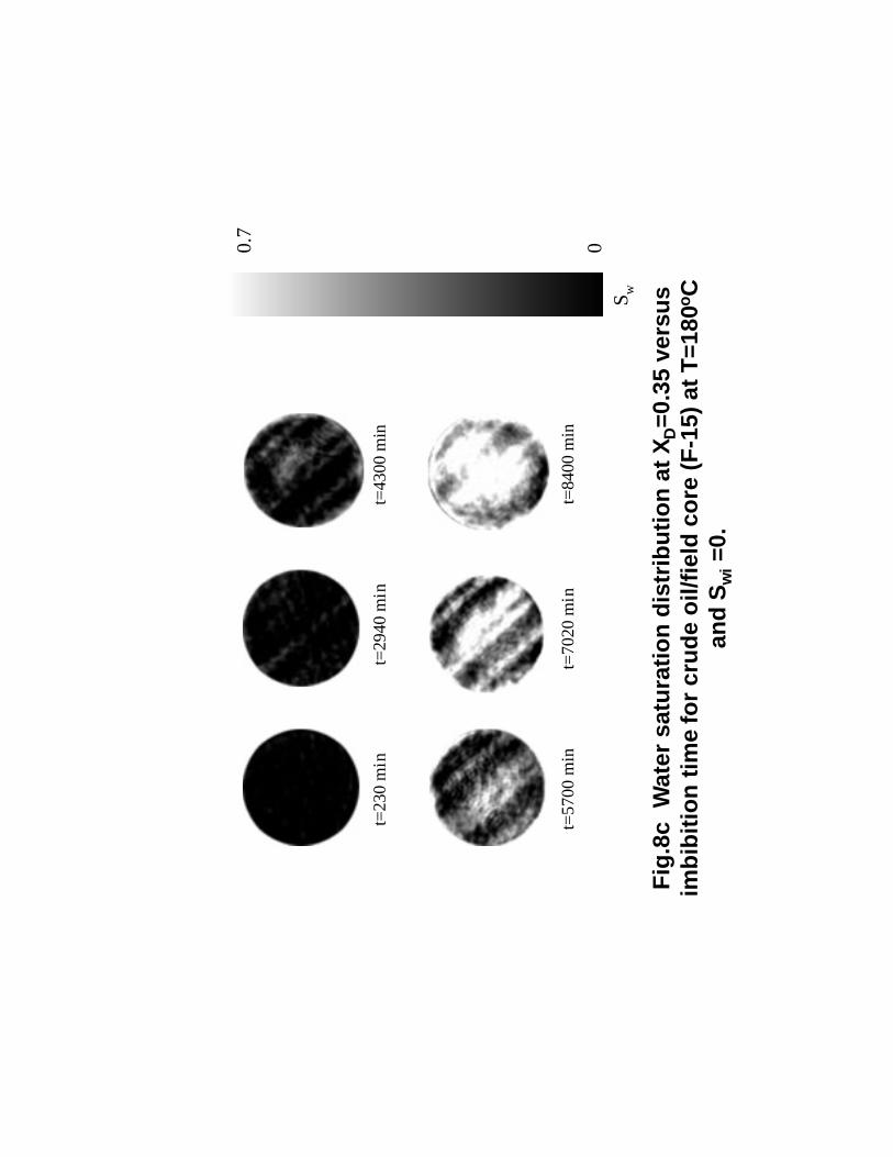
0.7

Sw

0

t=23

0 m

in

t=

2940

min

t

=43

00 m

in

t=

57

00

min

t=70

20 m

in

t=84

00 m

in

Fig

.8c

W

ate

r s

atu

rati

on

dis

trib

uti

on

at

XD=

0.3

5 v

ers

us

imb

ibit

ion

tim

e f

or

cru

de

oil

/fie

ld c

ore

(F

-15

) a

t T

=1

80

oC

an

d S

wi =

0.

0

0.1

0.2

0.3

0.4

0.5

0.6

0.7

0.8

0.91

00.1

0.2

0.3

0.4

0.5

0.6

0.7

0.8

0.9

1

Dim

en

sio

nle

ss L

en

gth

, X

D


t=351 m

int=

1041 m

in

t=2421 m

int=

2820 m

in

t=3840 m

int=

5700 m

in

t=7080 m

int=

8520 m

in

t=8760 m

int=

8940 m

in

t=10080 m

int=

11300 m

in

Fig

.9a

W

ate

r s

atu

rati

on

pro

file

fo

r w

ate

r im

bib

iio

n i

n o

il-f

ille

d f

ield

co

re

(F-2

5)

at

T=

18

0oC

: c

rud

e o

il (

da

sh

ed

lin

es

in

dic

ate

fo

rce

d i

mb

ibit

ion

).

Sw

i=30%

t=0

min

t=

2421

min

t=3

84

0 m

in

t

=57

00 m

in

t

=87

60

min

t

=89

40 m

in

t=10

080

min

Sw

0.7

0.3

Fig

.9b

. W

ate

r s

atu

rati

on

dis

trib

uti

on

at

XD=

0.3

2 v

ers

us t

ime f

or

cru

de

oil/f

ield

co

re (

F-2

5)

at

T=

180

oC

an

d S

wi=

30%

.

0.11

10

100

1000

Tem

pera

ture

(oC

)

Sorsi (PV)

n-d

eca

ne-o

utc

rop (

2)

bla

ndol-outc

rop (

2)

PA

O40-o

utc

rop (

1)

crude-o

utc

rop

crude-f

ield

Fig

.10

. C

orr

ela

tio

n b

etw

ee

n r

em

ain

ing

oil

sa

tura

tio

n a

nd

te

mp

era

ture

fo

r d

iato

mit

e c

ore

.

0

0.2

0.4

0.6

0.81

05

10

15

20

25

30

35

t D

Normalized Oil Recovery (fraction)

T=

22°C

, air

T=

88°C

, n-d

eca

ne

T=

22°C

, n-d

eca

ne

T=

180°C

, bla

ndol

T=

120°C

, bla

ndol

T=

57°C

, bla

ndol

T=

180°C

, P

AO

40

T=

120°C

, P

AO

40

Fig

.11

. S

ca

led

sp

on

tan

eo

us

wa

ter

imb

ibit

ion

in

oi-

fill

ed

ou

tcro

p d

iato

mit

ec

ore

at

ele

va

ted

te

mp

era

ture

s:

min

era

l o

ils

.

0

0.2

0.4

0.6

0.81

05

10

15

20

25

30

35

t D

Normalized oil recovery (fraction)

T=

180°C

, outc

rop a

t S

wi=

0

T=

120°C

, outc

rop a

t S

wi=

0

T=

180°C

, outc

rop a

t S

wi=

21.7

%

T=

180°C

, fie

ld (

F-1

5),

Sw

i=0, D

=920.4

ft

T=

120°C

, fie

ld (

F-2

), S

wi=

0, D

=685.3

ft

T=

180°C

, fie

ld (

F-2

5),

Sw

i=30%

, D

=920.8

ft

T=

180°C

, fie

ld (

F-1

), S

wi=

27.1

%,D

=681.3

ft

Fig

.12

. S

ca

led

sp

on

tan

eo

us

wa

ter

imb

ibit

ion

in

oil

-fil

led

dia

tom

ite

c

ore

s

at

ele

va

ted

te

mp

era

ture

s:

cru

de

oil

.

0.0

0E

+0

0

5.0

0E

-05

1.0

0E

-04

1.5

0E

-04

2.0

0E

-04

2.5

0E

-04

3.0

0E

-04

3.5

0E

-04

05

01

00

15

02

00

T (

oC

)

dΦim/dT (min-0.5

/o

C)m

odel,

with

wettability

alte

ratio

n

exp

erim

enta

l

model,

with

out w

ettability

alte

ratio

n

blan

dol

0.0

0E

+00

2.0

0E

-05

4.0

0E

-05

6.0

0E

-05

8.0

0E

-05

1.0

0E

-04

1.2

0E

-04

050

100

150

200

T (

oC

)

dΦim/dT (min-0.5

/o

C)

exp

erim

en

tal

mo

de

l, wi

th w

ettabili

ty a

ltera

tion

mo

de

l, wh

itho

ut

wettability

alte

ratio

n

0.0

0E

+00

2.0

0E

-05

4.0

0E

-05

6.0

0E

-05

8.0

0E

-05

1.0

0E

-04

1.2

0E

-04

1.4

0E

-04

1.6

0E

-04

050

100

150

200

250

T (

oC

)

dΦim/dT (min-0.5

/o

C)

mod

el,

with

wet

tabi

lity a

lter

atio

n

exp

erim

enta

l

mod

el,

witho

ut w

etta

bilt

iy a

lter

atio

n

0.0

0E

+0

0

5.0

0E

-06

1.0

0E

-05

1.5

0E

-05

2.0

0E

-05

2.5

0E

-05

3.0

0E

-05

3.5

0E

-05

4.0

0E

-05

05

01

00

15

02

00

25

0

T (

oC

)

dFim/dT (min-0.5

/o

C)

exp

erim

enta

l

model, w

ith w

ettabili

ty a

ltera

tion

model, w

itho

ut

wettabili

ty a

lte

ratio

n

Fig

.13

. E

ffe

ct

of

tem

pe

ratu

re o

n im

bib

itio

n p

ote

nti

al

for

wa

ter

imb

ibit

ion

in

oil

-fi

lle

d d

iato

mit

e c

ore

.(a)

nC

10/b

rin

e(b

) B

land

ol/b

rin

e

(c)

PA

O 4

0/b

rine

(d)

Cru

de

oil

/bri

ne

0

0.0

5

0.1

0.1

5

0.2

0.2

5

0.3

0.3

5

0.4

0.4

5

0500

1000

1500

2000

2500

3000

3500

4000

4500

t (m

in)

Oil recovery (PV)

befo

re fin

es

pro

duct

ion

after

fines p

roduct

ion

Fig

.14

. E

ffe

ct

of

fin

es

pro

du

cti

on

on

wa

ter

imb

ibit

ion

in

oil

sa

tura

ted

d

iato

mit

e c

ore

: n

-de

ca

ne

T=

25

oC

Sw

i=0

147

An Experimental Investigation of the Effect of Temperatureon Recovery of Heavy Oil From Diatomite

(Task 2b)

Introduction

The ultimate goal of this work is to improve our understanding of multiphase fluid andheat flow characteristics of low-permeability, fractured rock. Oil production from many low-permeability, fractured reservoirs is frustrated by not only low matrix permeability but also largeoil viscosity and a matrix wettability state that is not sufficiently water wet to favor waterimbibition during conventional water flooding (e.g., Al-Hadhrami and Blunt, 2001). Somediatomaceous reservoirs appear to exhibit these attributes. Thermal recovery using hydraulicallyfractured wells is one process to improve oil recovery and unlock these resources. Steam injectionin either drive (Kovscet et al., 1996a, 1996b), or cyclic modes (Murer et al., 2000; Kumar andBeatty, 1995) is being tested for light and heavy-oil diatomite reservoirs.

Virtually all recovery processes for diatomite, and other tight fractured rocks, rely to anextent on free and/or forced imbibition (Akin et al., 2000). Capillary phenomena are equallyimportant during steam injection into diatomite. Injected steam, especially at short times, isaccompanied by condensation and flow of the resulting hot water away from the injector. Insteam drive, a condensed hot-water bank precedes the steam zone within the reservoir; whereas,in cyclic steam operations the steam zone generally collapses during soak and production leavinga region filled with heated oil and condensed steam. A necessary precursor to elucidating thermaloil recovery processes in diatomite is to understand the imbibition characteristics of hot water.

Diatomite is relatively unstudied in the laboratory. Most previous studies were performedon sandstone (e.g., Bourbiaux and Kalaydijian, 2000; Jadhunandan and Morrow, 1991; Reis andCil, 1993; Tang and Morrow, 1997) or chalk (e.g., Cuiec et al., 1994; Milter and Øxnevard,1996) at low temperature. Diatomite is fine grained, exhibits a variety of pore length scales, andflow pathways are complex (Akin et al., 2000; Schwartz, 1988). Generalization of results acrossrock type from chalk or sandstone to diatomite is not currently possible. Further experimentsprobing the flow properties of this important class of rock are needed.

The first X-ray CT images of diatomite undergoing water injection were given by Wendelet al. (1998). Subsequently, spontaneous co-current (Akin et al., 2000) and counter-current (Zhouet al., 2002) imbibition characteristics were imaged with X-ray CT for a variety of mobilityratios, at room temperature. Regardless of imbibition mode, oil was recovered at the laboratoryscale at appreciable rates with sensibly zero pressure drop. On the other hand, Kamath et al.(1995) showed that water-oil relative permeability end points could be increased by as much as31% during forced displacement with increased flow rate and/or pressure drop.

This work studies experimentally the effect of temperature on water imbibition rate andultimate recovery from oil-saturated core using diatomite from an outcrop and a heavy-oil field.The paper proceeds by discussing imbibition potential. It is a necessary tool for consistent

148

interpretation of experimental results. Then, the high-pressure, high-temperature apparatusconstructed to conduct spontaneous and forced imbibition experiments is described. Recoverydata are interpreted using a dimensionless scaling group and an analytical model that exposes therole of wettability alteration, viscosity reduction, and oil/water interfacial tension.

Imbibition Potential

When gravity is negligible, spontaneous water imbibition in oil-saturated porous media isdriven solely by capillary pressure, Pc

Pc =

2σr

cosθ (1)

where σ is the interfacial tension between oil and water, r is the radius of curvature of theinterface, and θ is the water/oil/solid contact angle. When the rock is strongly water-wetting, thecontact angle is close to zero and interfacial tension dominates the capillary pressure for a givenporous medium. Because the interfacial tension decreases with increasing temperature,temperature usually decreases the capillary pressure. This has a negative effect on waterimbibition rate for a rock/water/oil system.

On the other hand, the viscosity of oil and water phases is a function of temperature.Recently, it was demonstrated that the counter-current water imbibition rate in oil saturatedporous media is expressed by Zhou et al. (2003) as,

uw = k1

µwµo

krokrw

M +1

M

dPcdx

(2)

where uw is the time and space dependent Darcy velocity, k is the permeability of the core, krw(Sw)and kro(1-Sw) are the relative permeability to water and oil, respectively, M (=µokrw/µwkro) is themobility ratio, and x is the axial distance. When temperature is increased, the oil-phase viscositydecreases and oil mobility improves. Thus, water imbibition as a function of temperature isgoverned by the competition between reduction in the viscosity of oil and water phases andinterfacial tension in the absence of any alteration in wettability. When oil-phase viscositydecreases more rapidly with temperature as compared to interfacial tension, the water imbibitionrate increases.

Because of the variation in physical properties with temperature (Al-Hadhrami and Blunt,2001; Tang and Morrow, 1997; Anderson, 1986; McCaffery, 1972; Rao, 1999; Tang andKovscek, 2002), interpretation of experimental results to follow is difficult without a quantitativetool accounting for the variation of interfacial tension, phase viscosities, and wettability withtemperature. The tool employed here is the imbibition potential (Akin et al., 2000; Tang andKovscek, 2002).

The imbibition potential derives from the work of Handy (1960) who demonstrated thatimbibed water volume is proportional to the square root of the time in air saturated sandstone

149

cores. Appendix A details a development similar to that of Handy, but accounting for the mobilityof the wetting and nonwetting phases. The origin for these relations is Eq. 2. In short, the analysisindicates that the slope of the line for imbibed water volume versus the square root of imbibitiontime is written

∆S w = Φimt0.5 (3)

where t is time, S w is the spatial average water saturation, and Φim is the imbibition potential.Equation 3 implies that the imbibition potential is analogous to rate when time is expressed as asquare root. Appendix A demonstrates that Φim is parameterized by capillary pressure, water andoil viscosity, relative permeability, and the absolute permeability.

Before proceeding, several comments are in order. Oil recovery curves in counter-currentimbibition do not necessarily follow square-root-of-time behavior (e.g., Miller and Øxnevard,1996; Parsons and Chaney, 1964; Lefebvre duPrey, 1978). If flow is counter-current at the porelevel, square-root-of-time behavior is generally not observed unless the nonwetting phase isinviscid. Additionally, the redistribution of fluids in the pore space is not instantaneous duringcounter-current imbibition. This is another possible cause for counter-current imbibition results todeviate from square-root-of-time behavior (cf. Barenblatt et al., 2002). Hence, before applyingEq. 3, we check carefully that the saturation trends versus the square root of time are linear.

Experimental

Experimentally, we wish to obtain the change of average water saturation, measure therate of imbibition, and determine fluid displacement patterns within the rock. X-ray CT meetsthese goals, is noninvasive, and measurements can be made without stopping an experiment.Figure 1 presents the experimental setup. The heart of the apparatus is a high-temperature, high-pressure coreholder. Experimental procedures minimize the effects of rock compaction andvolumetric expansion of fluids on oil recovery. Extensive details of the apparatus, cores, wettingand nonwetting fluids, and image processing of the raw CT data are presented in Appendix B.

Briefly, outcrop and field cores are both employed. Porosity of the samples ranges from0.55 to 0.67 while permeability varies from 0.8 to 2.9 md, as documented in Fig. 2 and Table 1.Field samples are cleaned before use, whereas outcrop core is not.

Three white oils (n-decane, blandol, and PAO40) and crude oil were used as the oilphases. The viscosity of these fluids at 22 °C varied from 0.93 to 6400 mPa-s. A relatively freshsynthetic brine with the composition reported in Table 2 was the aqueous phase. Figure 3 showsthe viscosity versus temperature relationships; note the dramatic effect of temperature on theviscous mineral and crude oils. Figure 4 reports interfacial tension versus temperature for thevarious fluids. Tension is extrapolated to high temperature as explained in Appendix B and Table3.

The apparatus, Fig. 1, is designed for both spontaneous countercurrent imbibition and co-current forced displacement. An initial condition is established and the coreholder brought to aconstant temperature. All tests are conducted isothermally. Tests are initiated with zero initial

150

water saturation, Swi, and with Swi of about 0.30. These different initial conditions bracket therange of observed saturation patterns within the core. At low Swi, a water front developscharacterized by a saturation pattern that becomes disperse over time, whereas at greater Swi moreuniform fill up of the porous medium with no discernable front is noticed (Akin et al., 2000).

Brine is supplied at one face of the core at 0.5 cm3/min. The outlet is kept closed andbrine imbibes countercurrently. Water is supplied until no further change in water saturation ismeasured by CT.


Results are described in order of increasing complexity, that is, from outcrop cores andsimple fluids to field cores and crude oil. The experimental program was designed to separate theeffects of viscosity reduction of oil and water phases from beneficial alteration of wettabilitytoward water wetness. In this manner, the magnitude of the principle mechanisms of thermalrecovery from diatomite is probed.

In total, 18 experiments are reported, Table 1. The average increase in aqueous phasesaturation versus the square root of time followed a linear trend as verified by the nearly unitvalues of correlation coefficient, R2. All lines were forced through the initial saturation. Hence,the imbibition potential is useful for sorting the macroscopic results. Table 1 summarizes allexperiments by listing the best-fit imbibition potential, the correlation coefficient of the fit, andvarious quantities of interest. Fortunately, the outcrop sample permeabilities are all nearly equalallowing generalization without considering the role of permeability. Also tabulated is remainingsaturation of the nonwetting phase after spontaneous imbibition, Sorsi.

The air-water/outcrop system exhibits the largest Φim consistent with low gas viscosityand the extreme preference of the solid surface for water as opposed to air. The fieldcore/water/heavy-oil at 43 °C exhibits the smallest. For each fluid system, the values of Φimpresented in Table 1 indicate that an increase in temperature results in more rapid recoveryconsistent with reduced oil and water viscosity as temperature increases. Similarly, at a fixedtemperature, the recovery rate decreases as the ratio of wetting to nonwetting phase viscositydecreases. Systems with initial water saturation also show lesser imbibition potential.

Outcrop Core/Water/Mineral Oil

Figure 5 shows recovery versus time for all outcrop core/water/mineral oil tests. We plotall data together for compactness and to emphasize the effectiveness of our scaling procedure tofollow. A general trend for outcrop cores is a decrease in imbibition rate, as the nonwetting-phaseviscosity increases. This observation is indicated by the time period for recovery in Fig. 5 and byimbibition potential in Table 1. There is some discrepancy in the ordering of imbibition potentialwith viscosity. For instance, compare water/blandol results with water/PAO40 results at 180 °C.The more viscous PAO40 has larger imbibition potential. As discussed later, this effect is tracedto different wettability among two different samples of quarry stone.

151

A second trend is that remaining oil saturation following spontaneous imbibitiondecreases as temperature increases, as shown by Table 1 and Fig. 5. Consider the runs withblandol, the modestly viscous mineral oil. The test temperatures were 57, 120, and 180 °C,respectively. The viscosity ratio of displacing phase (water) to displaced phase (oil) was about0.062 at 57°C, 0.15 at 120 °C, and 0.217 at 180 °C. Spontaneous imbibition recovery of blandolincreases with temperature. The final oil recovery is about 0.49 PV at 57 oC, 0.53 PV at 120 oC,and 0.62 PV at 180 oC.

Outcrop Core/Water/Crude Oil

To increase system complexity in a logical fashion, the heavy diatomite crude oil wasused next as the nonwetting phase in outcrop cores. A separate core was used for each test.Because the crude oil is very viscous at room temperature, the oil and coreholder were heated to80°C to accelerate the oil injection process. After the core was saturated with the crude oil, thecore was heated or cooled to test temperature and allowed to reach thermal equilibrium. Eachcore was aged with oil at the test temperature for 1 to 2 days before it was subjected to waterimbibition. The oil is heavy and asphaltenic. No effect of aging time is apparent in our work.

Figure 6 shows the oil recovery curves for the crude oil as a function of temperature. Allcrude oil tests are plotted on a single figure to emphasize the success of our scaling efforts tofollow. The average rate of imbibition for the outcrop/water/crude-oil system (dashed lines)increases by more than an order of magnitude as temperature increases from 42 to 180°C. The oilrecovery when Swi equals 0 and T equals 42 oC is only 0.03 PV; however, the final oil recovery isabout 0.42 PV at 180 oC when Swi equals 0. For the experiment conducted at 180 oC and Swiequal to 21.7%, the water imbibition rate for the core is initially (t < 1500 min) similar to the coreat T=180 oC and Swi=0. After 1500 min, water imbibition rate declines quickly indicating lessercapillary driving forces and greater flow resistance to oil production.

In-situ aqueous phase saturation profiles as a function of time are presented in Fig. 7 foran experiment at 180 °C with no initial water. Water propagates throughout the core. Theimbibition front is relatively diffuse. Water advance is slower compared to previous mineral-oilcases. At 180 °C, crude oil viscosity and the viscosity of the PAO40 are about the same. Yet, theoutcrop/water/crude oil system without intial water saturation takes about 4,000 min to reach astable water saturation profile. Experiments were halted when the water saturation profiledisplayed, sensibly, no change between subsequent CT exposures. Additionally, Fig. 7 indicatesthat the water saturation along the core is not uniform at the end of the experiment. Near the inletthe final water saturation is 0.55 PV, while near the outlet it is roughly 0.10 PV.

152

Field Core /Water/Crude Oil

Four field cores and crude oil were used for the remaining tests. The cores F-2 (685.3 ft),and F-15 (920.8 ft) were used at 43, 120, and 180 °C, and zero initial water saturation. The othertwo cores, F-25 (928.1 ft) and F-1 (681.3 ft), were used for experiments at 180 °C with initialwater saturations of 30 and 27%, respectively. Recovery versus time for these experiments (solidlines) is presented in Fig. 6.

The first test with F-2 at 43oC did not show any water imbibition. Hence, its imbibitionpotential is zero, Table 1. This core was then heated to 120oC and allowed to reach thermalequilibrium. Then it was subjected to water imbibition. Oil viscosity at 120 oC is reduced to 12mPa-s and the mobility ratio is more favorable (i.e., smaller). About 0.22 PV oil was produced byspontaneous water imbibition at 120oC.

The second field core (F-15) was used at 180oC and zero initial water saturation. Here, theoil viscosity is 4.5 mPa-s at test conditions. The water imbibition rate at times less than 500 minincreased significantly, as compared to results at 120 °C. The rate declined somewhat in the laterperiod, but it is still greater than rates for the 120 °C case. The final oil recovery is about 0.43 PV.

Figure 8 shows data obtained by X-ray CT for the experiments at 120 and 180°C. Theaqueous-phase saturation profiles in Fig. 8a teach that water imbibes instantly at 120 °C, for allpractical purposes. However, the imbibing front only progresses through a little more than onehalf of the core. After 7370 min, the shape and position of the displacing front no longer evolves.The region of relatively high water saturation near the center of the core indicates low oil relativepermeability. Combined with the somewhat elevated oil viscosity of 12 mPa-s at 120 °C, flowresistance is high. The nonwetting phase has difficulty exiting the interior of the core.

Figure 8b shows aqueous phase saturation profiles versus time for the 180 °C experiment.The displacement front is diffuse, but propagates throughout the entire core. At the end of theexperiment, the water saturation is somewhat larger near the inlet as compared to the outlet.Water saturation images versus time are displayed in Fig. 8c for the cross section XD=0.35 at 180°C. Dark shading indicates low Sw while light indicates high Sw. Due to core heterogeneity, thewater saturation is not uniform within the cross section at all times and water has not yet swept allof the cross-sectional area. It is apparent that water advance through some of the bedding layers isresponsible for a major portion of the imbibition response. Note the almost pure white shading inthese swept areas compared to the darker shading in the remainder of the cross section. As timeprogresses, the amount of white shading increases as water imbibes slowly into the unsweptareas.

Subsequent experiments were conducted with initial water saturation. To establish initialwater saturation, the coreholder was heated to 80 °C. This reduced oil viscosity so that oil waspumped easiliy into the brine-saturated core. After oil breakthrough, the flow direction wasreversed and oil was injected until no further water was produced. The produced water wascollected and used to estimate the initial water saturation. The cores were aged at roomtemperature for slightly different amounts of time: F-25 was aged for 10 days while F-1 was agedfor only 2 days, as a result of CT-scanner availability. Again, we note no effect of aging time forthis heavy, asphaltenic crude oil.

153

Recovery versus time is shown in Fig. 6. The total oil recovery by spontaneous waterimbibition is about 27% of OOIP for core F-25 and about 40% of OOIP for core F-1. At the endof spontaneous imbibition, the cores were subjected to forced imbibition. The inlet pressure wasabout 4.03 MPa (585 psia) and outlet pressure was about 3.89 MPa (565 psia). Hence, thepressure drop across the core was about 138 kPa (20 psi). Forced water imbibition continued forabout 2 days until no further oil was produced. The total oil recovery increased to about 52% ofOOIP for core F-25 and 54% of OOIP for core F-1. Desaturation by forced imbibition occurredquickly. Most of the additional oil was produced in less than 400 min. These results indicate thatthe oil saturation remaining after spontaneous imbibition is well connected.

Forced displacement is effective for the diatomite system; however, the pressure gradientis roughly 1.8 MPa/m (80 psi/ft). This is consistent with the results of Kamath et al. (1995). For areservoir system, the imposed pressure gradient will obviously be less and oil production willoccur by both spontaneous and forced water imbibition.

The water saturation profile along the core for the experiment with F-25 (Swi=30%) ispresented in Fig. 9. The dashed lines are for forced water imbibition. This figure shows that thewater-front is much more diffuse than that observed for the experiments without initial watersaturation. It also teaches that forced water imbibition (following free imbibition) does not resultin clearly defined water fronts or oil banks moving through the core. That is, the displacementremains diffuse throughout spontaneous and forced imbibition without the formation of a true oilbank. Figure 9b shows that water distribution within the cross section is more uniform, ascompared to Fig 8c. Nevertheless, bedding structures fill with water preferentially.

Remaining Oil Saturation

Figure 10 summarizes remaining oil saturation versus temperature for all systems.Clearly, Sorsi declines as T increases for each fluid-rock system. As oil becomes more viscous, theremaining oil saturation shifts toward large values.

In general, results for experiments with crude oil lag behind those for the white mineraloils. Remaining oil saturation is greater, for a given temperature, for experiments with crude oilas compared to those with mineral oil. This statement remains true even when crude oil andPAO40 viscosity are roughly equal at 180 °C. Additionally, the apparent slope of the linedescribing the decline in Sorsi with increasing T is less for crude oil. As discussed subsequently,this indicates possible interaction of crude-oil constituents with rock that alters wettability towardmixed wetness.

From the imbibition curves at 180 oC for the field core/water/crude oil system, we do notfind a systematic effect of initial water saturation on water imbibition rate. This may be caused bythe heterogeneity of the field cores and the small sample set. Nevertheless, the remaining oilsaturation is somewhat insensitive to the presence of initial water, Table 1. For the three cases at180 °C, Sorsi averages 0.51, and the largest Sorsi (=0.57) is found for the case where Sorsi is 0. Withforced water imbibition, the residual oil saturation could be as low as 0.35 PV.

154

Interpretation

Counter to expectation, results for the outcrop/water/mineral oil system appear to exhibitsome effects of changing wettability state versus temperature. Further, recovery results arequalitatively similar to our previous work at low temperature with the same rock15; however,imbibition rate is somewhat lower than expected for the experiments with blandol and n-decane.Compare Φim for blandol, n-decane, and PAO40 in Table 1. The more viscous PAO40 has largerΦim across a range of T.

Outcrop cores were cut from two different blocks of quarried stone. Most of theexperiments here were conducted with core from the second block and its wettability state differsfrom the first. To verify this statement, recovery versus time is scaled with appropriatedimensionless groups accounting for the effect of mobility ratio and interfacial tension, but notinitial wettability state. Separate characteristic curves are obtained because the initial rockwettability state differs among samples.

The focus of our interpretation efforts are on determining the magnitude of the shift inwettability toward water wetness. We deconvolve reduction in phase viscosity and interfacialtension from any increase in water wetness. A mechanism for wettability alteration is also given.

Scaling

Although several scaling groups for counter-current imbibition have been proposed (e.g.,Zhou et al., 2002; Zhang et al., 1996; Wang, 1999), we use exclusively our previously developedgroup (Zhou et al., 2002) resulting from Eq. 2,

tD =kφ

σ

Lc2

λ rw* λ rnw

* t

M * +1

M *

(4)

The mobility ratio is incorporated explicitly and the group originates from restriction ofthe equations of motion to counter-current flow. It is most appropriate given the extremevariations in viscosity and mobility with temperature. The term λ r

* = kr* /µ is a characteristic

mobility for the wetting (w) and non-wetting (nw) phases, and M* = λ rw* /λ rnw

* is a characteristicmobility ratio. End-point relative permeabilities are used for calculating *

rλ and *M . The scalingis explicitly for spontaneous imbibition and krw

* is properly evaluated at 1-Sorsi. Numerical valuesof kro

* and krw* are set equal to 0.60 and 0.16, respectively, consistent with previous work (Zhou

et al., 2002; Schembre and Kovscek, 2002).

The characteristic length scale, Lc, is expressed as,

Lc =Vb

Ail i

∑(5)

155

where Vb is the bulk volume of the rock sample, Ai is the area of a face open for imbibition in thei direction and li is the distance from the open face to the no-flow boundary in the i direction.

Tension measurements in Fig. 2 were extrapolated to the temperature of interest asdescribed in Appendix B and Table 3.

Figure 11 presents the results from renormalizing the spontaneous imbibition behavior ofthe mineral oil/water/outcrop core systems. Contrast with Fig. 5 and note that scaled resultsseparate clearly into two groups. The water/air/outcrop and water/PAO40/outcrop systems fallinto one group. In a dimensionless time of roughly 2 these systems achieve residual non-wettingphase saturation. This is consistent with our prior results of imbibition in very strongly waterwetting diatomite outcrop (Akin et al., 2000; Zhou et al., 2002).

The second group of results in Fig. 11 requires a dimensionless time of order 10 to cometo final oil saturation. The existence of two distinct groups within the dimensionless dataindicates that core samples are not uniform with respect to initial wettability state. Evidently, theair/water/outcrop and PAO40/water/outcrop systems are more strongly water wet than theremaining systems. This is consistent with the fact that cores were drawn from two differentblocks of the same outcrop. These blocks were quarried at different times and locations.

We also scaled the water imbibition data for crude-oil tests. The results are presented inFig.12. Obviously, the scaled experimental data for crude-oil systems are more scattered thanthose shown in Fig.11. The scaled data falls into at least two groups. All of the results for theoutcrop core/water/crude oil system collapse onto a single curve, within experimental error.Cores for these experiments all came from the second block and so collapse to a single curve, asexpected. The experimental results with field cores separate according to depth. Results fromcores taken at roughly 680 feet nearly fall onto the outcrop results. Results from the field corestaken at about 920 ft follow a different trend. These experiments require more than twice as longin a dimensionless sense to reach residual oil saturation.

Wettability Alteration

The scaling exercise demonstrated that there are at least two wettability states in theoutcrop samples and two lithologies in the reservoir core. However, the degree and importance ofchange in the wettability state with temperature is not readily demonstrated. For this task, weemploy the concept of imbibition potential.

Appendix A makes evident that imbibition potential is a function of viscosity, interfacialtension, wettability, mobility ratio, and rock properties when gravity is negligible. That is,

Φim=f(fµr , fσ , fw , fr) (6)

156

where fµr is the viscosity ratio function, fσ is an interfacial tension function, fw is the wettabilityfunction, and fr is the rock-property function. A differentiated form of imbibition potential withregard to temperature is

dΦimdT

=∂Φ im∂fµr

dfµrdT

+∂Φim∂fσ

dfσdT

+∂Φim∂fw

dfwdT

+∂Φim∂fr

dfrdT

(7)

where dΦim dT , dfµR dT , dfσ dT , dfw dT , and dfr dT are the imbibition potential, viscosity ratio(oil to water), interfacial tension, wettability, and rock-property variation with temperature. Theseterms are measured independently through experiments. The terms

∂Φ im ∂fµR , ∂Φ im ∂fσ ,

∂Φ im ∂fw , and ∂Φ im ∂fr represent the variation of the functionality of imbibition potential withchange in viscosity ratio, interfacial tension, wettability, and rock properties. We assume that theimbibition-potential functionality is constant, or is a very weak function of temperature and thefluids employed. The various partial derivatives in Eq. 7 are then constants. The followingdefinitions result:

a1 = ∂Φim ∂fµR , a2 = ∂Φim ∂fσ , a3 = ∂Φim ∂fw , and a4 = ∂Φim ∂fr , respectively.

Upon substitution, Eq. 7 reduces to

dΦimdT

= a1dfµrdT

+ a2dfσdT

+ a3dfwdT

+ a4dfrdT

(8)

When the factors, a1, a2, a3 and a4 are determined experimentally, or theoretically, the imbibitionpotential is predicted at different temperatures through integration of Eq. 8.

With the measured imbibition potentials in Table 1, viscosity in Fig. 3, and interfacialtension in Fig. 4 and Table 3, we obtained dΦim dT , dfµR dT , and dfσ dT functions. However,the variation of wettability with temperature for water/oil/diatomite is currently unknown.Diatomite is a siliceous rock; therefore, we employed the contact angle versus temperaturerelationship measured for water/mineral oils/quartz systems by McCaffery18 to determine the dfw dTfunction for outcrop/water/n-decane. The term dfr dTis set to 0, because the experimentalapparatus is designed to maintain a constant net confining stress regardless of temperature, and,accordingly, the effect of temperature on porosity and permeability is negligible.

Equation 8 is reduced to three terms with weight factors. By regressing the data for

dΦim dT , dfµR dT , dfσ dT , and dfw dT at three different temperatures for the diatomite/water/n-decane system, the weight factors a1, a2, and a3 are determined as 8.73×10-6 mPa-s-1-min-0.5, -5.74×10-4 cm/dyne-min0.5, 1.78×10-2 min-0.5, respectively. It was assumed that the measuredweight factors do not change with temperature and are valid for all water/oil/diatomite systems inthis study. This assumption is verified a posteriori.

One of the important implications of Eq. 8 is to identify wettability alteration withtemperature. The terms dΦim dT , dfµR dT , and dfσ dT are obtained through water imbibition

157

tests for various measured viscosity ratios and interfacial tension. The sole unknown effect is thatof wettability. If dfw dT is greater than 0 at a given temperature, wettability alteration occurs withan increase in temperature. The Φim versus T data shown in Table 1 are matched versustemperature for the water/Blandol, water/ PAO40, and water/crude oil systems by adjusting the dfw dT function. For simplicity, a linear relationship is assumed,

dfwdT

= mT + b (9)

Figure 13 displays the results of this exercise for the various experiments in outcrop core.All views in Fig. 13 present the variation in imbibition potential with wettability alterationincluded as a solid line. Results when wettability alteration is not accounted for (i.e., dfw dT = 0 )are given as dashed lines. Experimental data are given as symbols. Values of the best-fitcoefficients m and b are summarized in Table 4. Also tabulated is the percentage change inimbibition performance with increased temperature attributed to wettability. For water/n-decanethe temperature range of interest is 22 to 88 °C. For the remaining systems The temperature rangeof interest is 40 to 180 °C. All experiments in outcrop core exhibit some shift toward increasedwater wetness as temperature increases.

Figure 13a shows the imbibition potential variation with temperature obtained for thewater/n-decane/diatomite system. Model data (solid line) well fits the experimentally measureddata (symbols). Wettability alteration with temperature is significant for this system. Table 4reports that the wettability effect increased imbibition potential by roughly 30%. If wettabilityalteration is neglected altogether (dashed line), imbibition potential remains nearly unchangedwith increase in temperature. This suggests that reduction in viscosity ratio, which increasesimbibition potential is nearly offset by reduction in interfacial tension, that decreases imbibitionpotential. Recall that the core used for water/n-decane tests was not strongly water-wet initially;the remaining oil saturation decreased from 0.72 to 0.36 PV as temperature increased from 25 to88oC.

Figure 13b shows the measured and modeled imbibition potential variation versustemperature for outcrop/water/blandol. Compared to the water/n-decane/diatomite system, thewettability alteration with temperature is slightly less for the water/blandol/diatomite system,Table 4. When wettability alteration with temperature is omitted from the analysis, the imbibitionpotential increases with temperature as indicated in Fig. 13b. This result teaches that the decreasein viscosity ratio with temperature overcomes the negative effect of a decrease in interfacialtension at elevated temperature.

The modeled and measured imbibition potential data for the outcrop/water/PAO-40system are presented in Fig.13c. Table 4 shows only a 4% change in imbibition potential withtemperature that is attributed to wettability alteration for this system. The cores used for theseexperiments were strongly water-wet (the first sample of outcrop) as indicated by the scaledresults in Fig. 11. When the wettability alteration function is excluded from our analysis, thecalculated imbibition potential still demonstrates a significant increase with temperature. Thelines in Fig. 13c are nearly identical with and without wettability alteration. This indicates that the

158

majority of the increase in imbibition performance for the outcrop/water/PAO40 system is fromviscosity ratio reduction and improved oil mobility with temperature.

Figure 13d presents the imbibition potential data for the outcrop/water/crude-oil system.Table 4 teaches that the shift in wettability increased performance by more than 12%.Additionally, reduction in viscosity ratio plays a major role in improving imbibition potential,dashed line Fig. 13d. When wettability alteration is excluded from the interpretation, it is foundthat an increase in temperature still increased imbibition potential significantly. The wettabilityshift toward water wetness and the improvement in oil mobility both contributed significantly tothe oil recovery with an increase in temperature from 43 to 180 oC.

Unfortunately, a quantitative interpretation of the effects of wettability on the reservoircore/water/crude oil system is not possible. The data are too sparse and the 4 cores did not allbehave similarly in a nondimensional sense, Fig. 12. Nevertheless, the outcrop core/water/crudeoil results imply that both oil mobility improvement and wettability shift contribute to enhancedoil recovery in reservoir core.

The analysis summarized in Fig. 13 assumed that the coefficients a1, a2, and a3 wereconstant and independent of the fluids within the core. With the values of dfw/dT for each fluidsystem reported in Table 4, constancy of these coefficients across all fluid systems is checked.Numerical averages and the variation of each coefficient are a1 = 8.7×10-6 ± 0.03×10-6 mPa-s-1-min-0.5, a2 = -5.69×10-4 cm/dyne-min0.5± 0.16×10-4, and a3 = 0.0168 ± 0.0008 min-0.5. Withinexperimental error, these values are identical to the prior values of a1, a2, and a3. The assumptionof invariant coefficients is self consistent.

A Mechanism for Wettability Alteration

Recently, Al-Hadhrami and Blunt (2001) proposed a model to explain the wettabilityalteration encountered during thermal operations in fractured carbonate systems. They assumeddesorption of oil-wet asphaltene macromolecules from rock surfaces when the temperature wasover a critical value. Thus, water-wet surface was produced. Similar opinions were also expressedby Hjelmeland and Larrondo (1986). This mechanism is not likely for siliceous surfaces.Laboratory experience suggests asphaltenes adhere irreversibly and stably (Clementz, 1982; Yanet al., 1997). Strong organic-phase solvents, such as hot pyridine, are generally needed to dissolveasphaltenes adsorbed on siliceous solids (Windholz et al., 1976).

There are at least two mechanisms for increase in water wetness with temperature in theseexperiments. The white oils, especially n-decane, exhibit solvent action on cores. Recall that theoutcrop cores were dried but not cleaned. A fraction of the increase in water wetness with theoutcrop core/water/n-decane system is likely due to dissolution of dirt or organic contaminationon the rock surface. Simple cleaning action increases water wetness. Of course, experiments withcrude oil do not exhibit this effect.

A second, and field relevant, mechanism for increase in water wetness with temperature isfines detachment from rock surfaces. It is here that our efforts are concentrated. Oil-wet rock

159

surfaces and mixed wettability result when polar, asphaltenic components of crude oil adhere toreservoir solids in a fashion perhaps similar to that suggested by Kovscek et al. (1993). Anincrease in temperature destabilizes fines attached to rock surfaces through a reduction or changeof sign in colloidal attractive forces. Oil-coated fines cover the pore walls, but they are releasedfrom pore surfaces because colloidal adhesion forces decrease with increasing temperature. Fresh,water-wet rock surfaces underlying the fines are thereby exposed upon fines release. The increasein water-wet surface area results in an increase in water wetness for the entire core. In someregards, this mechanism is analogous to current thinking about wettability alterationaccompanying dilute brine injection at constant temperature (Tang and Morrow, 1999). Thefollowing experimental phenomena support this proposed mechanism.

It is observed experimentally that an increase in water imbibition efficiency at hightemperature is accompanied by fines production. Table 5 lists the feature of fines collected atvarious temperatures for counter-current water imbibition in oil (or air) saturated outcropdiatomite cores. Concurrent with an increase in oil production rate, appearance of fines in thecore effluent is observed. The higher the temperature, the greater the fines production. Also, it isfound that fines production correlates with nonwetting phase viscosity: the greater the oilviscosity the greater the fines production.

The size of produced fines tends to increase as the viscosity of the non-wetting phaseincreases. The total fines production during counter-current imbibition is about 98 mg for crudeoil and about 31 mg for blandol after 50 and 22 PV of hot water, respectively, were circulatedacross the core face. The cumulative imbibed water was about 0.43 PV for the crude oil test and0.61 PV for blandol test. For water imbibition in air-saturated cores, we did not observe visiblefines production.

The color of the fines transitions from light-yellow to brown as the non-wetting phase isswitched from mineral oil to crude oil. In the case of crude oil, this implies that the fines adsorbedsome polar oil components, such as asphaltenes and/or resins. When a drop of crude oil wasplaced into the produced solution containing fines and the solution was agitated, the oil dropdisappeared quickly due to adsorption onto fines. Hence, these fines had affinity for oil and werepossibly oil-wet.

To study further the above hypothesis, additional water imbibition experiments in n-decane-saturated diatomite were conducted using a single core. The core was saturated with n-decane and subjected to water imbibition at room temperature until no obvious oil productionoccurred. The oil recovery was about 0.28 PV and no visible fines were produced.

Thereafter, the temperature was raised to 90oC and forced displacement was performed(∆p=5 psi/cm). More oil was produced accompanied with some fines production (about 27 mgwith size less than 3µ). The final oil recovery was about 0.67 PV after forced water imbibition.Next, the fluids in the core were removed by applying house vacuum at T=60oC.

After the core was dry and cold, it was re-saturated with n-decane and again subjected tospontaneous water imbibition at room temperature. The results are presented in Fig. 14. One findsthat both water imbibition rate and the extent of oil recovery are improved after some finesproduction from this core. The permeability prior to fines production is 3.32 md, whereas it is

160

2.71 md following fines production. As the permeability decreased by about 18%, the increasedwater imbibition rate cannot be ascribed to an increase in permeability. The final oil recovery tospontaneous imbibition increases from 0.25 PV to about 0.4 PV after fines production; themodified Amott index is 0.37 before fines production and is 0.60 after fines production indicatinga more water-wet state.

Because the temperature is the same for these two imbibition tests, we infer that theincrease in imbibition efficiency is due to increase in water-wetness induced by hot-waterinjection and some fines production. The imbibition potential is 0.0047 min-0.5 for the firstexperiment and increases to 0.0077 min-0.5 following fines production.

Conclusions

Temperature affects profoundly water imbibition and oil recovery from oil-filleddiatomite, a tight fractured siliceous rock. Imbibition rate increases and the remaining oilsaturation to spontaneous imbibition of water decreases systematically with increasingtemperature. Forced displacement, following spontaneous imbibition recovered significant oil. Infield core, recovery increased from roughly 30 % of OOIP following spontaneous imbibition ofwater to 50% with forced displacement.

Experiments are interpreted using imbibition potential. It is defined as the best-fit slopeobtained from plotting average water saturation versus the square root of time. Imbibitionpotential is divided into contributions from viscosity ratio, interfacial tension, wettability, androck properties. Imbibition results depend strongly on the initial wettability state of the rock.When the rock/water/oil system is initially strongly water wet, recovery performance increaseswith temperature mainly because oil viscosity decreases. On the other hand, when the rock is notstrongly water wet, an increase in temperature also leads to an increase in water wetness and thisaids imbibition performance too. There is competition between the beneficial effects of anincrease in water-wetness and oil mobility as compared to the detrimental effect of decreasinginterfacial tension with temperature. Over the range of temperatures examined here, wettabilityand mobility ratio improvements are dominant.

Production of oil-wet fines was observed at high temperature along with a correspondingincrease in water imbibition rate and extent of oil recovery. It is proposed that wettabilityalteration at high temperature is related to fines detachment from pore surfaces. Detachmentcreates water-wet surfaces when the rock is siliceous.

Significantly, a scaling analysis correlated experimental results. The scaling group isphysically-based; it incorporates mobility ratio, end-point wetting and nonwetting phasemobilities, and remaining oil saturation to spontaneous imbibition as a function of temperature.Thus, scale up of imbibition behavior from the laboratory conditions to thermal field operationsappears feasible.

161

Nomenclature

a constants in Eq. 12A area, cm2

b constant in Eq. 13, °C-1

C0,C1 constants in corresponding statesrelationship for interfacial tension

CT CT number, Hounsfieldsf functionk permeability, md kr permeabilityL length, mm slope in Eq. 13, °C-2

M mobility ratioPc capillary pressure, PaPV pore volumer characteristic radius, mS saturation, fractionSorsi remaining oil saturation after spontaneous

imbibitionT temperature, oCTc critical temperature, Kt time, s or minx distance, mXD dimensionless length, fractionV volume, cm3

Greek Symbolsφ porosity, fractionΦim imbibition potential, min-0.5

σ interfacial tension, N/mλ mobilityθ contact angle

Subscripts and Superscriptsa airc characteristico oilr rockw water, wettabilityµr viscosity ratio

162

References

Akin, S., Schembre, S.K., Bhat, S.K., and Kovscek, A.R., “Spontaneous ImbibitionCharacteristics of Diatomite,” J. Pet. Sci. and Eng. 25 (2000) 149-165.

Al-Hadhrami, H.S., and Blunt, M.J., “Thermally Induced Wettability Alteration to Improve OilRecovery in Fractured Reservoirs,” Soc. Pet. Eng. Res. Eval. & Eng (June 2001) 179-186.

Anderson, W.G., "Wettability Literature Survey-Part 2: Wettability Measurement," JPT(November 1986) 1246-1262.

Barenblatt, G.I., Patzek, T.W., and Silin, D.B., “The Mathematical Model of Non-EquilibriumEffects in Water-Oil Displacement,” paper SPE 75169 presented at the 2002 SPE/DOESymposium on Improved Oil Recovery, Tulsa, OK, April 13-17.

Birdi, K. S, ed. "Handbook of Surface and Colloid Chemistry," CRC Press, New York (1999).

Bourbiaux, B.J. and Kalaydjian, F.J., “Experimental Study of Cocurrent and CountercurrentFlows in Natural Porous Media,” Soc. Pet. Eng. Res. Eval. & Eng. (August 2000) 361-368.

Carslaw, H. S. and Jaegar, J. C., Conduction of Heat in Solids, 2nd Edition, Oxford UniversityPress, Oxford: (1959) 297-326.

Clementz, D. M., "Alteration of Rock Properties by Adsorption of Petroleum Heavy Ends:Implication for Enhanced Oil Recovery," paper SPE 10683 presented at 1982 SPE/DOESymposium on Enhanced Oil Recovery, Tulsa, OK, April 4-7.

Cuiec, L., Bourbiaux, J.B. and Kalaydjian, F.J., “Oil Recovery by Imbibition in LowPermeability Chalk,” SPEFE (September 1994) 200-208.

Handy, L.L., “Determination of Effective Capillary Pressure for Porous Media from ImbibitionData,” Trans, AIME 219 (1960) 75-87.

Hjelmeland, O.S. and Larrondo, L.E., "Experimental Investigation of the Effects of Temperature,Pressure, and Crude Oil Composition on Interfacial Tension Properties,” SPEFE (July1986) 321-328.

Jadhunandan P.P and Morrow, N.R., “Spontaneous Imbibition of Water by Crude Oil/Brine/RockSystems,” In Situ 15(4) (1991) 319-345.

Kamath, J., deZabala, E.F., and Boyer, R.E., “Water/Oil Relative Permeability Endpoints ofIntermediate-Wet, Low-Permeability Rocks,” SPEFE (March 1995) 4-10.

163

Kovscek, A.R., Johnston, R.M., and Patzek, T.W., “Interpretation of Hydrofracture GeometryDuring Steam Injection Using Temperature Transients I. Model Formulation andVerification,” In Situ 20(3) (1996A) 251-288.

Kovscek, A.R., Johnston, R.M., and Patzek, T.W., “Interpretation of Hydrofracture GeometryDuring Steam Injection Using Temperature Transients I. Model Formulation andVerification,” In Situ 20(3) (1996B) 289-309.

Kovscek, A.R., Wong, H., and Radke, C.J., “A Pore-Level Scenario for the Development ofMixed Wettability in Oil Reservoirs,” Am. Inst. Chem. Eng. J. (June, 1993) 1072-1085.

Kumar, M., and Beatty, F.D., “Cyclic Steaming in Heavy Oil Diatomite,” paper SPE 29623presented at the 1995 SPE Western Regional Meeting, Bakersfield, CA, March 8-10.

Lefebvre Du Prey, E., “Gravity and Capillarity Effects on Imbibition in Porous Media,” SPEJ(June 1978) 195-206.

Lide, D. R., ed., “Handbook of Chemistry and Physics,”, 81st edition, CRC Press, New York,(2000).

McCaffery, F.G., "Measurement of Interfacial Tension and Contact Angles at High Temperatureand Pressure," J. Can. Pet Tech. (July-September 1972) 26-32.

Milter, J. and Øxnevard, R.I., , “Spontaneous Imbibition in Two Different Chalks Facies,”Petroleum Geoscience 2, (1996) 231-240.

Murer, A.S., McClennen, K.L., Ellison, T.K., Larson, D.C., Timmer, R.S., Thomsen, M.A., andWolcott, K.D., “Steam Injection Project in Heavy-Oil Diatomite,” Soc. Pet. Eng. Res.Eval. & Eng (February 2000) 2-12.

Parsons, R. W. and Chaney P.R., “Imbibition Model Studies on Water-Wet Carbonate Rocks,”SPEJ (March 1964) 26-34.

Prats, M, Thermal Recovery, 2nd Printing, Society of Petroleum Engineers, Dallas, TX: (1986)220.

Rao, D. N., "Wettability Effects in Thermal Recovery Operations," Soc. Pet. Eng. Res. Eval. &Eng (October 1999) 420-430.

Reid, R.C., Prausnitz, J.M., and Poling, B.E., “The Properties of Gases and Liquids,” McGraw-Hill, New York (1987).

Reis, J.C. and Cil, M., “A Model for Oil Expulsion by Counter-Current Water Imbibition inRocks: One Dimensional Geometry,” J. Pet. Sci. and Eng, 10 (1993) 97-107.

164

Ross, C.M. and Kovscek, A.R., “Pore Microstructure and Field Distribution in a DiatomaceousReservoir,” paper SPE 75190 presented at the 2002 SPE/DOE Symposium on ImprovedOil Recovery, Tulsa, OK, April 13-17.

Schembre, J. M. and Kovscek, A.R. "A Technique for Measuring Two-Phase RelativePermeability in Porous Media via X-ray CT-Measurments," J. Pet. Sci and Eng 39(1-2)(2002) 159-174.

Schwartz, D.E.: “Characterizing the Lithology, Petrophysical Properties, and Depositional Settingof the Belridge Diatomite, South Belridge Field, Kern, County, California,” in Studies ofthe Geology of the San Joaquin Basin, S.A. Graham and H.C. Olson (eds.), The PacificSection of Society of Economic Paleontologists and Mineralogists, Los Angles, CA(1988) 281-301.

Tang, G. and Kovscek, A.R., "Experimental Study of Heavy Oil Production from Diatomite byWater Imbibition at Elevated Temperatures," paper SPE 75132 presented at the 2002SPE/DOE Thirteenth Symposium on Improved Oil Recovery held in Tulsa, OK., April13-17.

Tang, G., and Morrow, N.R., “Effect of Temperature, Salinity and Oil Composition on WettingBehavior and Oil Recovery by Waterflooding;” Soc. Pet. Eng. Res. Eval. & Eng, (1997) .

Tang, G.-Q. and Morrow, N. R, “Influence of Brine Composition and Fines Migration onCrude/Oil/Brine/Rock Interactions and Oil Recovery,” J. Pet. Sci. and Eng. 24 (1999) 99-111.

Wang, R. “Gas Recovery from Porous Media by Spontaneous Imbibition of Liquid,”, MS thesis,University of Wyoming, Laramie, WY 82070 (1999).

Wendel, D.J., Kunkel, L.A., and Swanson, G.S., “Waterflood Potential of Diatomite: NewLaboratory Methods,” paper SPE 17439 presented at the 1998 SPE California RegionalMeeting held in Long Beach, CA, March 23-25.

Windholz, M., Budavari, S., Stroumtsos, L. Y., and Fertig, M. N. eds, The Merck Index, NinthEdition, MerckandCo. Inc., Rahway, NJ: (1976) 1033.

Withjack, E.M., “Computed Tomography for Rock Property Determination and Fluid FlowVisualization,” SPEFE (December 1988) 696-704.

Yan, J., Plancher, H., and Morrow, N. R., "Wettability Changes Induced by Adsorption ofAsphaltenes," paper SPE 37232 presented at the 1997 SPE International Symposium onOilfield Chemistry, Houston, TX., February. 18-21.

Zhang, X., Morrow, N.R., and Ma, S., “Experimental Verification of a Modified Scaling Groupfor Spontaneous Imbibition,” SPERE (November 1996) 280-285.

165

Zhou, D, Jia, L. Kamath, J., and Kovscek, A.R., “Scaling of Counter-Current ImbibitionProcesses in Low-Permeability Porous Media,” J. Pet. Sci. and Eng, 33 (2002) 61-74.

166

Appendix A–Imbibition Potential

The object of this appendix is to substantiate the functionality given in Eq. 3 where thevolume of water imbibed is proportional to the square root of time. We develop approximaterelations for both a frontal advance like pattern of water movement and a diffusive pattern of corefill up. The second object is to draw out the parameters that influence the magnitude of theproportionality constant.

The Bond number (=(ρw-ρo)gk/σ) for water-oil displacement here is of the order 10-10

assuming a k of 3 md, interfacial tension of 15 mN/m, and a density difference of 200 kg/m3.Buoyancy is negligible in comparison to capillarity.

A frontal advance analysis similar to Handy's (1960) begins with the assumption of one-dimensional fluid flow, the capillary pressure varies linearly with x (i.e., dPc/dx=∆Pc/x), andstrictly counter-current flow as described by Eq. 2. Next, substitute uw (= 1 φA( )dVw dt ) to obtain

uw =1Aφ

dVwdt

= k1

µwµo

krwkro

M +1M

∆Pcx

(A1)

where Vw is the volume of water imbibed. In a frontal-advance analysis, the volume of waterimbibed is related to the position of a front by mass balance according to

x =Vw

φA(1 − Sorsi )(A2)

Upon substituting Eq. A2 into Eq. A1, simplifying, separation of variables, and integration,

Vw2 = 2k

(φA)2(1 − Sorsi)µwµo

krwkro

M +1M

∆Pct (A3)

The volume of water imbibed is converted to the increase in the core-averaged aqueous-phasesaturation after division by pore volume (∆S w = Vw / φAL ). After conversion of Vw to ∆S w andtaking the square root of the resulting expression, we obtain

∆S w

= (2k(1 − Sorsi )

µwµo

krwkro

M +1M

∆PcL2 )0.5 t0.5 (A3)

Equation A3 teaches that the volume of water imbibed versus time is a function of water and oilviscosity, interfacial tension, wettability, mobility ratio, and rock properties.

167

It is arguable that a frontal advance analysis for imbibition may over simplify processphysics. Some experimental data display a slow diffuse-like fill up for cores subjected to water.Alternately, we begin by stating continuity for the aqueous phase,

∂Sw∂t

+1φ

∂uw∂x

= 0 (A4)

where constant porosity and incompressibility is assumed. Substituting Eq. 2 of the main text foruw and employing the equality ∂Pc / ∂x = (∂Pc / ∂Sw)(∂Sw /dx) yields,

∂Sw∂t

+∂∂x

D(Sw)∂Sw∂x

= 0 (A4)

where D(Sw) is the hydraulic diffusivity expressed as

D(Sw ) =kφ

1µwµo

krwkro

M +1M

∂Pc∂Sw

(A5)

Equation A4 is a second order, nonlinear, partial differential equation. Note the similarity to thediffusion equation. Solution of Eq. A4 is nontrivial. A simplifying assumption is that a constanteffective hydraulic diffusivity, Deff, is obtained by evaluating D(Sw) at some constantrepresentative value. The assumption of constant hydraulic diffusivity allows straightforwardanalytical solution. The resulting expression (Carslaw and Jaegar, 1959) is

Sw( x, t) = (1 − Sorsi )erfc(x

2 Deff t) (A6)

where erfc denotes the complementary error function.

The volume of water imbibed as a function of time is obtained upon integrating the waterflux at the core inlet.

Vw = AφDeff∂Sw(x,t )

∂x0

t∫

x=0dτ (A7)

Application of a Laplace Transform to the intergral yields

∂Sw (x, t)∂x0

t∫

x=0dτ =

1s

(1 − Sorsi )Deff s

(A8)

where s is the Laplace transform of t. Substitution of Eq. A8 into Eq. A7 and application of theLaplace back-transform results in

Vw = 2AφDeff0.5(1 − Sorsi )

tπ

(A9)

168

Again, we convert the volume of water imbibed to the increase in the average water saturation ofthe core to obtain

∆S w =2(1 − Sorsi)Deff

0.5

L πt (A10)

Equations A10 and A3 derive from substantially different analyses. Nevertheless, theydisplay similarly that the change in the average water saturation is proportional to the square rootof time. Further, the proportionality constant is parameterized by capillary pressure, phasemobilities, phase viscosity, and relative permeability.

169

Appendix B–Experimental Details

This appendix details the experimental apparatus, fluids and fluid properties, and theprocedures for the experiments and processing of data. Significant care was exercised in thechoice of materials and in apparatus design, Figure 1. The major components of the apparatus aredescribed next.

Coreholder

We fabricated a coreholder that resembles a Hassler-sleeve from aluminum (6061-T6). Itis relatively transparent to X-rays and therefore CT-scanable. Cores with lengths from 2.5 to 7.5cm (1 to 3 in) and 2.5 cm (1 in) diameter can be held. The apparatus is assembled by coating thecore with a thin film of silicone gel (Ultra Copper High Temp RTV Silicone Gasket Maker) andplacing the core inside PTFE heat-shrink tubing (Plastic Professional). The silicone-gel isnonwetting and does not penetrate the core. It serves to prevent any fluid bypass during injectiononce a confining pressure is applied; thus, the silicone gel-tubing combination serves as a high-temperature sleeve.

Mineral oil is used as a confining fluid in the annular space between the sleeve and thealuminum coreholder. A net confining pressure of roughly 1.4 MPa (200 psi) is applied. Heatingtape is wrapped around the outside of the coreholder and then covered with high-temperatureinsulation. A temperature controller maintains constant coreholder temperature. Thethermocouple for feedback to the controller is located in the center coreholder between thecoreholder and the heating tape. This system was designed and tested for service up to 260°C(500 °F) and a maximum total confining pressure of 7 MPa (1,000 psia). In addition to beingcompatible with a CT scanner, the main advantage of this design is that the effect of heating onrock compaction and fluid expansion is minimized. The system is brought to the temperature ofinterest at a constant difference between confining and pore pressure while fluids flow throughthe core.

The endcap contacting the core face contains fluid distribution channels of largedimension (order mm) that allow water to be circulated across that face. The pressure drop forfluid flow through the endcap is sensibly zero.

The coreholder is attached to an L-shaped mounting bracket. This assembly is bolted to astepper-motor driven precision positioning system (Compumotor RP240, Parker-Hannifin) that isused to position the core inside the CT gantry. Any position along the length of the core can berevisited with an accuracy of ±0.01 mm.

CT Scanner

The scanner is a fourth generation Picker 1200SX with a scan angle of 398°. The voxeldimension is 0.35 mm by 0.35 mm by 3 mm. The tube current is 95 mA and the energy level of

170

the radiation is 130 keV. The acquisition time of one image is roughly 6 s, while the processingtime is about 40 s. Images are acquired in series and processing delayed until all the desiredimages are acquired. Thus, the total acquisition time to scan the length of the core is short enoughto characterize the saturation profile along the core at a particular time.

Rock

Both field and outcrop cores are studied. All rock samples are in the opal-A phase.Outcrop diatomite cores (Grefco Quarry, Lompoc, CA) have a porosity, φ, of 62-67% and an airpermeability, k, of 2-4 md, as shown in Table 1. They are almost pure white and the porosity isrelatively uniform, as shown by the representative CT image in Fig.2a. This quarried diatomiterepresents an end member of so-called "clean" reservoir rock resulting from Late Miocenediatomaceous sediments (Ross and Kovscek, 2002). It provides a convenient and appropriatecontrast to the reservoir samples used here. A previous study (Akin et al., 2000) characterizedfully water-wet samples. We used a similar process to cut and shape the outcrop diatomite coresamples as described in Akin et al. (2000) and Zhou et al. (2002). Our previous study did notsuggest a need to clean outcrop samples. The cores were not cleaned but dried and preserved inan oven under house vacuum at a temperature of 50-60 °C.

Field cores are from a heavy-oil field (Kern Co., CA). Only 4 samples were available.Core recovery from diatomite fields is frustratingly poor. Their porosity ranges from 55 to 59 %and permeability from 0.8 to 1.3 md, as indicated by Table 1. The field cores were sampled fromdepths between 650 to 980 ft: F-1 depth=681.3 ft, F-2 depth = 685.3 ft, F-15 depth=920.8 ft, andF-25 depth=928.1 ft. Cores were cleaned by injecting a mixture of methanol and toluene. Aftercleaning, they were preserved in synthetic reservoir brine and sealed in an airtight aluminum baguntil used. The composition of the synthetic brine is listed in Table 2. Prior to an experiment, thebrine was removed by drying carefully at 35 oC under house vacuum to avoid inducing fractures.Measurement of permeability after drying verified that cores had not fractured, see Table 1.Figures 2b to 2d show representative porosity images obtained for the field cores. Bedding andbanding structures are obvious. The length of the field cores was about 4.0 to 6.5 cm (1.6 to 2.6in) and the diameter was 2.5 cm (1 in).

Fluids

Three white oils, n-decane, blandol (Witco Chemical), and PAO40 (Chevron Lubricants),and filtered/dewatered heavy crude oil were used as the oil phases. The viscosity at roomtemperature (22 °C) for these oils is 0.93 mPa-s, 35 mPa-s, 407 mPa-s, and 6,400 mPa-s,respectively. The n-decane was chosen because it has a viscosity similar to water for a range oftemperature. In the next stages, a modestly viscous mineral oil, blandol, and more viscous PAO40were used. Hence, the viscosity ratio is made progressively less favorable (µw/µnw <1). The chiefreason for using the mineral oils was to identify the effect of temperature on recovery due to oilviscosity reduction without contribution to recovery from wettability alteration via crude oil-brine-rock interaction. It is shown in the main text that this goal was not entirely realized. Lastly,

171

we used crude oil to study further water imbibition behavior that could be attributed to bothreduction of oil viscosity and wettability alteration accompanying an increase in temperature.

Figure 3 shows the measured viscosity versus temperature relationship for the oils and forwater. It shows that the crude oil is the most sensitive to temperature. The viscosities of n-decaneand water versus temperature were obtained from Lide (2000). Oil viscosity was measured with aBrookfield (LVT) viscometer. The synthetic reservoir brine in Table 2 was used as the waterphase for all tests. It was prepared by dissolving salts in house distilled water. This dilute brinehas the same viscosity versus temperature relation as pure water (Prats, 1986).

The interfacial tension between oil and water at various temperatures was measured usinga Fisher Surface Tensiometer (Model 20). The liquids were preheated in an oven and then placedin the chamber for measurement. Due to the limitation of this instrument, we were only able tomeasure the IFT at temperatures below 80oC, as shown in Fig.4. The data were used to estimatethe tension as a function of temperature with the following corresponding states relationship(Birdi, 1986; Reid et al., 1987),

σ =Co(1 −

TTc

)C1 (B1)

where σ is the interfacial tension (N/m), T is the temperature (K), C0 and C1 are constants, and Tcis the pseudocritical temperature (K) of the oil and water mixture. The numerical value of C1 isset to 1.22 (Reid et al., 1987). When extrapolating σ data at T1 to σ at T2, a ratio (σ(T1):σ(T2)) isconstructed so that the coefficient C0 is eliminated. The mixture pseudocritical temperatures arethen obtained by regression of the data in Fig. 3. The Tc for n-decane-water, blandol-water,PAO40-water, and crude oil-water systems are taken as 568, 580, 584, and 598 K, respectively.Thereafter, we estimated the interfacial tension at temperatures outside the range of measurement.

Procedure

Figure 1 shows the complete experimental apparatus. Brine flows past one face of the coreat 0.5 cm3/min via pump (reciprocating or syringe pump at high temperature). We study counter-current behavior so the outlet of the coreholder was closed for all tests during the spontaneousimbibition phase. A backpressure regulator (model R3A-C, N-norgren Inc) elevated the systempressure to range between 2.7 and 4.1 MPa (400 to 600 psia) such that water remained in theliquid phase throughout the duration of an experiment. The confining pressure was set from 4.1MPa to 5.5 MPa (600 to 800 psia) so as to maintain roughly 1.4 MPa (200 psia) of net effectivestress. All experiments were conducted under isothermal conditions.

Produced oil was collected in a graduated cylinder to provide a check on the mass balanceand average water saturation as measured by X-ray CT scanning. After the produced water wasseparated from the oil, it was returned to a 300 cm3 water cylinder maintained at the experimentaltemperature.

172

The core was placed horizontally within the CT scanner gantry, as indicated by Fig.1.Cylindrical volume sections were monitored at 5 mm intervals along the central axis of the core.About 8 to 10 images were collected sequentially to span the core from inlet to outlet at anyparticular time. For the tests with an initial water saturation of zero, images of the dry air-saturated cores were taken first. Then oil was injected into the core until 100% saturated with oiland a second set of images acquired. The voxel-by-voxel values of porosity were calculated(Withjack, 1988) as,

φ =

CTor − CTarCTo −CTa

(B2)

where CT represents CT number (Hounsfields). The subscripts or and ar signify oil-saturatedrock and air saturated rock, respectively; whereas o and a represent the oil and air bulk fluidphases. Average core porosity is obtained by averaging porosity across each cross section andthen averaging cross-sectional porosities.

Once the initial condition was established, the core was subjected to counter-current waterimbibition. Water was supplied at the core face until no further change in water saturation wasmeasured by CT. The voxel-by-voxel water saturation, Sw, of each cross-sectional area wascomputed using6

Sw =

CTowr −CTorφ(CTw − CTo)

(B3)

where φ is the independently measured porosity from Eq. B2, the subscript owr refers to rockcontaining oil and water, the subscript w denotes the bulk water phase. One-dimensionalsaturation profiles were obtained by averaging the voxel-by-voxel Sw images from a cross section.Average water saturation within the core, S w , was obtained by averaging all of the cross-sectionalSw.

For the tests with nonzero Swi, images of the dry air-saturated cores were taken first. Thenthe core was 100% saturated with water and a second set of images was acquired. Thereafter, oilwas injected into the core to establish initial water saturation. The flow direction was reversedseveral times to obtain a uniform saturation distribution. When the initial water saturation wasestablished, a third set of images were taken.

173

Area 3. Mechanisms of Primary Heavy Oil Recovery

So-called cold production of heavy oil is attractive because steam injection iscostly due to the operating and capital expenses for steam generation facilities.Sometimes primary recovery can be on the order of 10-15% from heavy-oil reservoirs.Most cases of significant cold production are associated with foamy crude oil andhorizontal wells. Here, gas released from solution during pressure depletion remainsdispersed as small bubbles rather than uniting to form a single phase. With foamy crudeoil, the gas-oil ratio (GOR) is lower and the oil productivity of a well is increased overthe unfoamed case.

A key to developing a mechanistic understanding of foamy-oil behavior is todelineate bubble growth, interaction, and flow mechanisms at the pore level. These wererelatively unknown for foamy heavy oil at the start of this project. We used two-dimensional micromodels with one to one representation of sandstone pore features toobserve bubble size, nucleation, growth, and flow. The micromodels were subjected to adeclining pressure and the dynamics of heavy-oil solution gas drive observed. By usingvarious types of oil, we hope to delineate crude-oil conditions that are conducive to theformation of foamy oil. As pressure and temperature are important to crude-oil behavior,a major portion of the micromodel effort will be in the design of temperature controlledpressure vessel to conduct experiments at relevant temperatures and pressures. The majordifficulty is the construction of an apparatus that provides a confining pressure to themicromodel and incorporates a transparent window for viewing the micromodel. Thethickness of window, transparent confining fluid, and micromodel must remain thin forimaging with a high-power microscope objective. This work is summarized in the sectionentitled “A Microvisual Study of Solution Gas Drive Mechanisms in Viscous Oils.”

Companion experiments were also conducted in sands and sandstone. Thepurpose of the experiments was to measure the evolution of oil and gas saturation in situas well as pressure while undergoing primary production of foaming and non-foamingheavy crude oils. Production rate was varied to delineate critical rates of productionnecessary for foamy oil generation. Details in this subarea are entitled “Heavy OilSolution Gas Drive: Effect of Oil Composition and Rock Consolidation.”

Additionally, the experimental observations and results from the above weretranslated into a mechanistic model for cold production of heavy oil. The model ismechanistic and consistent with physical observations. Because unfoamed oil is a subsetof foamy oil, the model addresses primary production of all heavy crudes. Information onfoam-bubble size and the rheology of bubble-laden crude oil has been translated into amodel and subsequently tested in a reservoir simulator. Our approach is based on abubble population balance. In a population-balance method, the number density ofbubbles (i.e., the number of bubbles per unit volume of gas) is tracked as a function oflocation and time. Number density is also referred to as bubble texture. This section isentitled, “Model and Simulation of Cold Production Using a Population BalanceApproach.”

174

A Microvisual Study of Solution Gas Drive Mechanisms in Viscous Oils

(Task 3a)

Introduction

Primary production from some heavy-oil reservoirs operating under a solution-gas-drivemechanism exhibits unexpectedly high primary recovery with relatively low pressure declinerate, lower than expected producing gas oil ratios, and higher oil production rates. (Bora et al.,1997). The process of solution gas drive involves nucleation of gas bubbles as the pressure in thereservoir falls below the bubble point. It is postulated that these small bubbles are trapped andtend to remain dispersed in the oil for a relatively long period of time. Initial development ofheavy-oil reservoirs under solution-gas drive has economic advantage because implementation oftraditional thermal methods can be avoided or delayed, resulting in cost savings. For example, atFrog Lake, Alberta Canada, a study (Huang et al., 1997) concluded that cold production, thesimultaneous production of oil and sand with the aid of progressive cavity pumps, can produceheavy oil (12o API, 20,000 to 50,000 cP) without the introduction of any external thermal energy.Another study in the Hamaca area of the Orinoco Belt in Eastern Venezuela (De Mirabal et al.,1996, 1997) attributed the 10% OOIP (original oil in place) recovery to foamy-oil behavior of thecrude. It was postulated that the primary production mechanism of the Hamaca reservoirs iscontrolled by the in-situ formation of a non-aqueous, oil-continuous foam under solution gasdrive conditions. Notably, recovery in this case was obtained without sand production.

To explain the above phenomena a number of mechanisms have been suggested that canbe divided into two main categories. Geomechanical effects such as sand dilation anddevelopment of wormholes comprise the first category (Dusseault, 1993; Tremblay et al., 1999).Higher oil production rate with sand mobilization may lead to enhanced well drainage radius,grain movement, and gas bubble expansion. The second category suggests that the specialproperties of the flowing fluids, the gas and heavy oil, are the main reasons for high production(Pooladi-Darvish and Firoozabadi, 1999; Firoozabadi, 2001). These categories are not mutuallyexclusive.

In either event, retention of the evolved gas phase in the oil leads to maintenance of thereservoir energy. Although Dake (1978) does not explicitly discuss heavy oils, the generalmaterial balance equation is applicable to primary recovery by solution gas drive:

RF =

Bo − Boi( )+ Rsi − Rs( )Bg

Bo + Rp − Rs( )Bg

(1)

where RF is the fraction of the OOIP recovered, B is the formation volume factor, the subscripts oand g refer to oil and gas phases, respectively, and R is the gas-oil ratio. The subscripts s and sirefer to the solution gas-oil ratio and its initial value whereas the subscript p refers to thecumulative gas-oil ratio of the oil and gas produced. For heavy oils, Bo is close to 1 and varieslittle with pressure and/or the amount of gas in solution. Hence, the terms related to gas-oil ratio

175

determine RF. Equation 1 is inversely proportional to Rp- RS. Thus, systems where the cumulativegas-oil ratio differs little from the solution gas-oil ratio, all other factors being equal, obtainmaximum oil production. Gas that remains in the reservoir enhances the total reservoir systemcompressibility and results in greater cumulative production for a given pressure drop betweenthe well and the reservoir. It is our postulate that gas is retained because it coalesces slowly andremains dispersed as bubbles that are on the order of pore-size dimensions.

The work presented here is directed towards developing a better understanding of thecoalescence of bubbles during solution gas drive behavior in heavy oils. Specifically, we wish tounderstand the effect of oil-phase viscosity on the coalescence of gas bubbles trapped by narrowpore throats. Broadly speaking, bubble coalescence during solution gas drive is divided into twotime regimes. The first is governed by the diffusion of gas through oil to bubbles, whereas thelater is governed by pressure depletion and volumetric expansion that drains oil from betweenbubbles (Arora and Kovscek, 2000, 2003). The paper proceeds by discussing further the effect ofoil-phase viscosity on these two regimes. This motivates additional experimental study of,especially, the late-time regime. A microvisual apparatus employing etched-silicon micromodelsis then described along with results for bubble nucleation, growth, and coalescence. Discussionand conclusions round out the manuscript.

Dynamics of Bubble Growth in Porous Media

In bulk solution, gas nuclei appear due to thermal fluctuations when the pressure is belowthe bubble point (Scriven, 1959; Wilt, 1986). For gas/oil systems, homogeneous nucleationrequires a supersaturation of several thousand kPa provided that the system is not close to critical(Kamath and Boyer, 1995). Supersaturation is the difference between the liquid-phase pressure atwhich liquid and gas are in equilibrium and the actual liquid-phase pressure. In porous media,values of supersaturation are not large, compared to bulk solution, indicating heterogeneousnucleation (Kamath and Boyer, 1995). Nucleation sites, pore-wall topology and capillary forcesin combination with diffusion characteristics, such as the competition for solute between bubbles,determine the gas-phase occupancy of a porous medium.

There are two principal conceptual models for pressure and volume evolution duringsolution gas drive: (i) instantaneous nucleation (IN�Firoozabadi and Kashchiev, 1996) and (ii)heterogeneous nucleation in a progressive fashion (PN�Li and Yortsos, 1995). Instantaneousnucleation assumes that all bubbles nucleate from randomly located active sites at essentially thesame time. Bubbles are not modeled as originating from preexisting bubbles trapped in crevicesor the roughness of pore walls (Firoozabadi, 1997). Diffusional bubble growth is modeled asthree-dimensional with shape factors to account for nonspherical bubble shapes. It follows thatbubbles grow in a compact fashion such that bubbles are of roughly equal size throughout theporous medium.

On the other hand, PN assumes that bubbles are released from sites such as crevices orroughness on pore walls with poor liquid wetting characteristics. These sites become activatedwhen the local supersaturation exceeds the capillary pressure of the site. Because the size of suchcrevices holding trapped gas varies, bubbles are released from pore walls at different degrees ofsupersaturation, that is progressively as the supersaturation increases. Bubbles grow as a result of

176

diffusional transport of gas; however, the scaling of bubble growth in porous media is different ascompared to bulk due to the underlying pore microstructure (Li and Yortsos, 1995; Satik et al.,1995). Bubble growth is complicated by the geometry of pore space, the availability of solute,and the pressure gradient.

El Yousfi et al. (1997) undertook a series of experiments in transparent two-dimensionalrepresentations of pore space (i.e., micromodels) to differentiate among the IN or PN model.They saturated the micromodels with a solution of carbon dioxide in water. Bubbles werenucleated at a fixed supersaturation by connecting the micromodel to a gas reservoir maintainedat a pressure significantly less than the initial pressure of the micromodel (300 kPa). Bubblesappeared progressively for a period of time when the pressure drop became sufficient toovercome capillary forces. Later, bubbles grew by diffusion and expansion of total volume. Theseries of events described is more similar to PN than to IN especially in regard to the release ofpreexisting small bubbles from pore walls. However, the duration of bubble production (1 hour)was about 15% of the length of time required to deplete the micromodel of pressure. Hence, theystated that the process might be approximated by IN if the longer time behavior is of interest.Subsequently, Arora and Kovscek (2001, 2003) implemented a bubble population balance modelof solution gas drive incorporating PN physics. They found that the period of active bubblenucleation during pressure depletion was relatively short for the experiments modeled. In theircalculations, the supersaturation was always nonzero, but increased only during the initial stagesof pressure depletion. Their results supported the truncated progressive nucleation observationsmade by El Yousfi et al. (1997).

Diffusion-Dominated Coalescence

To study the role of oil-phase viscosity during the early diffusion controlled period ofbubble growth and coalsecence, we employ the IN model (Firoozabadi and Kashchiev, 1996).This choice is made simply because it is relatively easy to expose the role of viscosityquantitatively within IN. Alternately, the PN model should lead to similar conclusions withrespect to the role of viscosity on bubble growth and coalescence, but the time scaling may bedifferent.

Equations 4-12 of Firoozabadi and Kashchiev (1996) are used to develop a first orderdifferential equation (Eq. 13 of Firoozabadi and Kashchiev, 1996) for the volume of gas evolved.The equation is solved here with the Runge-Kutta method (Press et al., 1992). The diffusioncoefficient plays a role in setting the kinetic constant (Eq. A4 of Firoozabadi and Kashchiev.(1996) for bubble growth. The infinitely-dilute, mutual binary diffusion coefficient, DAB, iscalculated for our work using the empirical correlation of Hayduk and Minhas (1982),

DAB = 13.3×10−8 T1.47µε

VA0.71

(2)

where T is the absolute temperature, µ is the viscosity, VA is the molar volume, and the subscriptsA and B represent the solute and solvent, respectively. According to Reid et al. (1987), DAB can

177

be assumed to be a representative diffusion coefficient for concentrations of A as large as 10mole percent. We assume for calculations that CH4 is the solute dissolved in oil. The exponent εis given by

ε =

10.2VA

−0.791 (3)

From Tyn and Calus (1975), molar volume is estimated according to

VA = 0.285VC1.048 (4)

The critical volume, VC, of methane is 270 cm3. A temperature of 37.8 oC and bubblepointpressure of 28.44 bars are taken for calculations. Figure 1 illustrates that the diffusion coefficientdecreases by an order of magnitude as oil-phase viscosity increases from 100 to 1000 cP, all otherfactors being equal.

0.E+00

2.E-07

4.E-07

6.E-07

8.E-07

1.E-06

1.E-06

1.E-06

2.E-06

2.E-06

0 200 400 600 800 1000

Oil Viscosity (cP)

Diffu

sion

Coe

ffici

ent (

cm2/

sec)

Figure 1. Variation in diffusion coefficient of CH4 with oil viscosity.

Additional parameter choices for bubble growth calculations include: a pressure depletionrate of 5 bar/day, 5 bubbles nucleated per cm3 of liquid, and initial bubble radius of 1 µm. Otherparameters are used as specified by Firoozabadi and Kashchiev (1996). Note again that thediffusion coefficient enters into the kinetic constant determining the rate of bubble growth. The

178

growth of gas bubble volume as a function of time is calculated for oils with viscosities of 51, 95,178, 450, and 950 cP. Results are presented in Fig. 2. Viscosity plays an important role indefining the coalescence dynamics of gas bubbles during the early diffusion dominated stage.Bubble volume increases much more slowly in viscous oils compared to light oils chiefly becausegas diffuses much more slowly through viscous oil. In Fig. 2, it is clear that roughly doubling theoil-phase viscosity from 51 to 95 cP more than halves the volume of a bubble at a given time.

0

2

4

6

8

10

12

14

16

0 50 100 150 200

Time (minutes)

Gas

Pha

se V

olum

e (1

E-6

cc) 51 cP

95 cP178 cP490 cP950 cP

Figure 2. Variation in gas phase volume with time (constant pressure decline rate).

Pressure-Driven Coalescence

At times significantly later than bubble nucleation, coalescence is controlled mainly bythe pressure drop across bubbles that results from flow of oil and volumetric expansion ofbubbles. The liquid drains from thick-liquid bridges between bubbles, until they come closeenough to coalesce. A physical model is developed next to illustrate the role of solution viscosityon the coalescence of gas bubbles.

Consider Fig. 3 to understand a possible geometry of bubbles trapped inside a pore. Sucha configuration might arise in porous media if (i) the right bubble is held in place by a pore throatand the left bubble is driven forward, (ii) the bubbles are arrayed in a channel that isperpendicular to the flow direction such that the resulting pressure drop drives both bubblestoward one another, or (iii) the bubbles are oriented vertically and the lower bubble rises underthe forces of buoyancy. In Fig. 3, oil is the wetting phase, gas is the non-wetting phase, and thereis no aqueous phase present. The pore has a noncircular cross-sectional area, such as a triangle orsquare, Fig. 3b. Noaxisymmetric, cornered cross-sectional areas reflect the corners, nooks, andcrannies of real pores in porous media. Diffusional bubble growth at this stage is slow and

179

neglected. The flow of oil out of the lens occurs through the bulk oil held by capillarity in thepore corners. Transport through the oil films that line the straight section of the bubble-pore wallinterface is ignored. Flow resistance in thin films is inversely proportional to film thickness to thethird power; film flow is highly resistive compared to the bulk flow of liquids in corners. Anyeffect of gravity is ignored at the pore level. Finally, we assume that no thin-film forces arepresent to stabilize gas-oil interfaces.

(a)

oil in corners

thin film

(b)

aαθ

b

gas

gas gasFz

r oil

z = 0z = H(t)

Figure 3(a) Side view of two gas bubbles moving towards each other in a narrow pore;(b) cross-sectional view showing wetting-liquid distribution in a square pore

and illustrating the geometry of the corner flow problem.

The domain is divided in half by virtue of symmetry, as illustrated in Fig. 3. Thisdescribes coalescence scenario (i) or (ii) above. The plane of symmetry is a no-flow boundary. Atthis point, the problem becomes analogous to a �squeeze film� (Denn, 1980). Gas bubbles move

180

towards the symmetry plane and the oil flows out through the pore corners. The boundaryconditions are

vz = vr = 0 (5)

at the symmetry plane, where vz is the liquid velocity in the z direction and vr represents velocityin the r direction. The oil-gas bubble interface moves towards the symmetry plane, with velocityV(t). Therefore, at the moving surface( z = H(t)):

vz = V(t ) (6) vr = 0 (7)

The creeping flow approximation to the Navier Stokes equations is appropriate to the geometryand boundary conditions. The relevant equations are (Denn, 1980)

vr =

3rzV(t)H2(t )

1−z

H(t)

(8)

V(t) = −

dHdt

=2F

3πµR4

H

3 (9)

where H(t) is the distance between the symmetry plane and the bubble front at time t, µ is theviscosity of the wetting fluid, F, is the net imposed force at the surface represented by H(t), and Ris the effective radius of the bubble in the pore cross section. The effective radius is related to theprojected cross-sectional area, Ap, of the gas-liquid interfaces as R = (Ap /π)0.5.

The task now is to calculate the time needed for the two bubbles separated by distance Ho,to drain the oil lens so that coalescence may occur. Solution of Eq. 9 and some rearrangement,exposes the time dependence explicitly:

t =

3πµR4

4F

1H2(t)

−1

Ho2

(10)

In the above equation R, H, and Ho can be measured and quantified from visual micromodelexperiments, to follow. The viscosity of the oil, µ, is readily measured. The only unknown thatneeds additional mathematical treatment is the imposed force F.

The net force, F, is the net pressure drop pressure times the projected cross-sectional areaof the gas-liquid interface of the bubble:

F = (∆P− ∆Pc )Ap (11)

181

where ∆P is the pressure drop across the bubble and ∆Pc is the pressure drop for oil flow in thefour pore corners. The resistance to flow in the pore corners opposes thinning of the lens. Theexpression for the term ∆Pc is (Ransohoff and Radke,1988)

∆Pc =

qwµβLa2A w

(12)

where qw is the volumetric oil flow rate through the corners, β is the dimensionless flowresistance coefficient, L is the length of the bubble, Aw is the area of the corners occupied by theoil, and a is the interfacial radius of curvature, as shown in Fig 3b. The volumetric flow rate qwout of the oil lens is obtained by integrating Eq. 8 over the wetted perimeter times the thickness ofthe lens and back substituting V(t) from Eq. 9 to yield

qw =

6πR2V(t)H2(t )

z2

2−

z3

3H(t )

=

2FH3(t )3µR2

(13)

Now substituting this result for qw into the expression for ∆Pc in Eq. 12 gives

∆Pc =

2FH3(t )βL3a2R2Aw

(14)

Finally substituting Eq. 11 into Eq. 14 to eliminate F and rearranging results in

∆Pc =

λ(t )1+ λ(t )

∆P (15)

where

λ(t ) =

2πH3(t)βL3a2Aw

(16)

At this point, the relationship is established between ∆P and ∆Pc and the time required todrain the oil lens is calculable. An example illustrates the effect of oil viscosity on bubblecoalescence in the pressure-driven regime, Fig. 4. The pore cross section is taken as square; theradius, b, of the largest circle that may be inscribed within the square is 10 µm. Fluid viscosity isset to 1, 51, 95, 178, 490, and 950 cP. The bubble length and lens thickness are set 100 µm and50 µm, respectively. For a no-slip condition, sharp corner, zero degree contact angle, and squarepore, the theoretical value of β is 93.93 (Ransohoff and Radke, 1988). The value of ∆p is taken as1.4 KPa (0.2 psi) to correspond approximately with the micromodel experiments to follow. Thevalue for interfacial radius, a, is calculated from the work of Ransohoff et al. (1987). Theytabulate values for the equilibrium dimensionless interfacial entry curvature, Cdm = Cmb, in avariety of noncircular cross sections. For a square cross-section, Cdm equals 1.89. For a poreradius of (b=) 10.0 µm, the interfacial radius of curvature in the cross section illustrated in Fig.3(b) equals (a =b/ Cdm) 5.29 µm. The area wetted by the oil at the four corners, Aw, is related to

182

interfacial radius a by the geometric expression Aw = 4a2(1− π/ 4) . A zero degree contact angleis assumed. For the pore dimensions above, Aw equals 24.0 µm2. This detail to obtain theinterfacial radius of curvature and wetted area is necessary because cornered pores allow bubblesto adopt equilibrium entry curvatures that are slightly smaller than 2/b corresponding to ahemispherical bubble (cf. Ransohoff et al, 1987). For a square pore, it follows that the projectedcross-sectional area of the gas-liquid interface is (=4b2-Aw) 376. µm2. Consequently, the effectiveradius of the bubble in the square pore is ( = ((4b2 − Aw ) π)0.5) 11.0 µm.

0.01 0.1 1 10 100

5

10

15

20

25

30

time (seconds)

lens

thic

knes

s (µµ µµm

)

1 mPa-s

51 mPa-s

95 mPa-s178 mPa-s

490 mPa-s950 mPa-s

Figure 4. Example calculation illustrating the effect of oil viscosity onpressure-driven coalescence of two gas bubbles in a cornered capillary.

Figure 4 presents lens thickness versus time for this example. A logarithmic scale is usedbecause times for thinning vary substantially over the three orders of magnitude of µ. The timeinterval for coalescence is found by computing time versus interface position according to Eq. 10from the initial position to 1µm of separation. The solution is then extrapolated to an interfaceseparation of zero. At small thickness of the oil lens, the squeeze-film approximation predictsinfinite coalescence times. Thin-film forces at small thickness, however, determine ultimatelyfilm instability. Figure 4 does plot the thin-film portion but this part of the solution is obscured by

183

the solution for the thinning of the lens. Note that the time required for coalescence in Fig. 4increases considerably with oil viscosity. The times are relatively short because the pressure dropacross the bubble is rather large and translates to 14 MPa/m (600 psi/ft). This pressure drop,however, is consistent with the micromodel experiments to follow. To understand the role ofviscosity on bubble coalescence at field conditions, assume that the field gradient is 22.6 KPa/m(1 psi/ft). Then, the times in Fig. 4 increase by a factor of roughly 500.

Experimental

The experimental apparatus for this study consists of the micromodel, pressure vessel,optical equipment, and a system of hardware that controls fluid flow and pressure, as shown inFig. 5. For some experiments, a cornered glass capillary is substituted for the micromodel, asdescribed shortly. Etched-silicon-wafer micromodels of the type developed by Hornbrook et al.(1991) were used. The micromodels contain a 50 mm by 50 mm etched pore pattern as illustratedin Fig. 6. There are two etched inlet/outlet ports at opposite corners of the pore network. Holesare drilled into the silicon wafer at these ports to provide locations that allow fluid to enter andexit the micromodel. These micromodels contain a modification introduced by Castanier andSagar (1998): narrow etched channels adjacent to the edges of the pore network carry fluid to theinlet/outlet ports as shown in Fig. 6. The result is approximately linear flow, as opposed to radialflow, near the inlet and outlet of the micromodel. The porosity of the micromodel is roughly 0.2.The permeability of the micromodel is approximately 0.1 mD.

The etched side of a silicon wafer is bonded anodically to a borosilicate glass plate inorder to produce a micromodel. The silicon wafer is placed on an anode. The glass plate rests ontop of the silicon wafer. A cathode is placed on top of the glass plate. The system is heated to 600°F and the electrodes are charged to 1000 V after alignment of the micromodel and cover plate onthe bonding apparatus. During the heating process the pore surfaces of the silicon wafer areoxidized because they are in the presence of air at high temperature. The optimum bonding timeis one hour.

Pressure Vessel

The anodic bond that holds the etched-silicon-wafer to the glass cover plate can generallysustain a difference between internal and external pressure of about 30 psi. In order to achievesolution gas drive experiments at elevated pressures, a pressure vessel to hold micromodels wasdesigned and constructed, Fig. 5(b). The pressure vessel has a maximum design operatingpressure of 1000 psig and is temperature controllable. The apparatus as built was pressure testedto 940 psi without leaks or failure.

184

Pressure Vessel Lid

Sapphire Window

Micromodel

Pressure Vessel

Micromodel Fluid Inlet/Outlet

Confining Liquid Inlet/Outlet

O-Ring Gland

O-Ring Gland

(a)

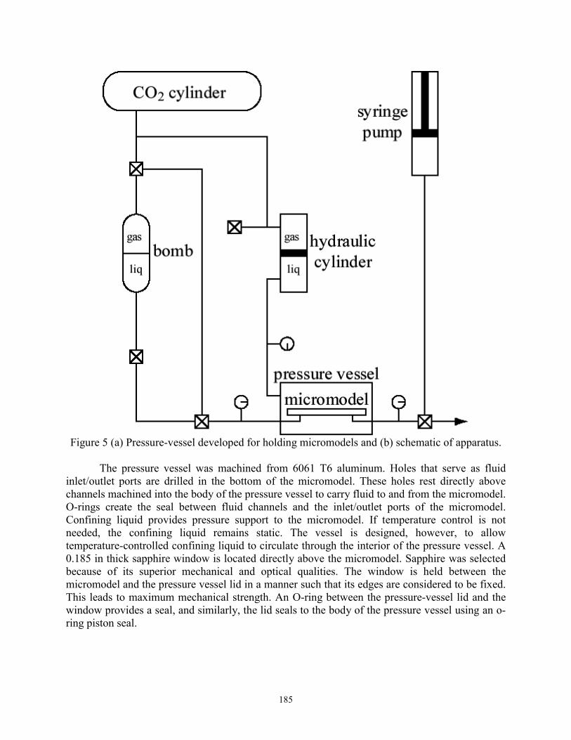
185

Figure 5 (a) Pressure-vessel developed for holding micromodels and (b) schematic of apparatus.

The pressure vessel was machined from 6061 T6 aluminum. Holes that serve as fluidinlet/outlet ports are drilled in the bottom of the micromodel. These holes rest directly abovechannels machined into the body of the pressure vessel to carry fluid to and from the micromodel.O-rings create the seal between fluid channels and the inlet/outlet ports of the micromodel.Confining liquid provides pressure support to the micromodel. If temperature control is notneeded, the confining liquid remains static. The vessel is designed, however, to allowtemperature-controlled confining liquid to circulate through the interior of the pressure vessel. A0.185 in thick sapphire window is located directly above the micromodel. Sapphire was selectedbecause of its superior mechanical and optical qualities. The window is held between themicromodel and the pressure vessel lid in a manner such that its edges are considered to be fixed.This leads to maximum mechanical strength. An O-ring between the pressure-vessel lid and thewindow provides a seal, and similarly, the lid seals to the body of the pressure vessel using an o-ring piston seal.

186

Optics

A microscope (Nikon, Optiphot-M) with a photo tube that allows for the connection of avideo camera was used. The silicon-wafer micromodels are opaque. Consequently, they areilluminated with an internal light source routed through the microscope objective and monitoredusing reflected light. A high-quality color video camera (PULNiX, TMC-7RGB, Sunnyvale, CA)is connected to the photo tube. Images are sent from the video camera to a VCR for recording. Anextra-long working distance objective lens (Nikon, MPLAN-20 0.4 ELWD) was used. Totalmagnification is 200X. The thickness of the sapphire window (4.7 mm), combined with thethickness of the micromodel cover glass (1 mm), results in a total cover glass thickness of 5.7mm. Some image quality is lost, mainly due to a loss in contrast.

The superior mechanical strength and optical qualities of sapphire provide the advantagesof a short working distance and high transmission of light. Sapphire, however, has anisotropicoptical properties. This sometimes causes double refraction images depending on the orientationof the window. In some cases, the image of the micromodel contains �phantom images� due tothis double refraction. Although the phantom images reduce image quality, the image remainseasily interpretable.

Pressure and Fluid Delivery Systems

Carbon dioxide from a high-pressure cylinder is used to pressurize confining water. Toavoid carbonating the confining water, it is pressurized in a modified hydraulic cylinder (MillerFluid Power, HV50R2N, Bensenville, IL) as shown in Fig. 5(a). A piston in the hydrauliccylinder separates the pressurized gas from the confining water. A gauge indicates the pressure ofthe confining liquid.

On the upstream side of the micromodel, a set of three-way valves allows CO2, dead oil,or oil saturated with CO2 to be pushed through the micromodel. Gas from a pressurized cylinderprovides drive energy. On the downstream side, a three-way valve selects whether the outlet isconnected to a syringe pump (ISCO, 100DM, Lincoln, NE), or to backpressure. The smallmicromodel volume of 0.015 mL necessitates the capability to withdraw fluid at very low rates.The syringe pump provides this capability, as it has a minimum refill rate of 0.0001 mL/min.Pressure gauges indicate the pressures upstream and downstream of the micromodel.

The apparatus is prepared for an experiment by assembling it and fastening the lid to thebody of the pressure vessel. Copious quantities of bone-dry CO2 are flushed through themicromodel to dry any residual moisture. Back pressure is applied and the gas pressure isincreased to the value desired for an experiment. Gas-saturated liquid prepared in a bomb, at thepressure of interest, is then introduced to the micromodel. This fluid is driven by increasing thepressure of the gas in the bomb. Any residual gas (CO2) phase dissolves readily in the fluid (oil orwater) and is thereby displaced. The valve is then closed that connects the micromodel to fluidsupply so that experiments can be run in depletion mode.

187

(a) (b)

Figure 6(a) Schematic of top view of micromodel illustrating injection and productionports and channels and (b) scanning electron microphotograph of micromodeletched pore pattern at 500X magnification.

Capillary Tube Experiment

Micromodel experiments as employed here, have two significant flaws when analyzingcoalescence. The first problem is with the control of events within a micromodel. It is hard tocapture frequently a situation where one can observe bubble coalescence under pressure gradientacross the bubble. Second, and most importantly, it is impossible to characterize exactly theforces acting on bubbles. Capillary tube experiments provide a suitable alternative for exploringsome aspects of the physics of bubble coalescence.

188

oil lens

gas bubble

gas bubble

1 mm

(a)(b)

Figure 7(a) Schematic of capillary tube apparatus for gravity-driven drainageof oil lens and (b) optical microphotograph of triangular capillarycross section.

Triangular capillaries with sharp corners were used to conduct the experiments. Theexperimental setup is shown in Fig. 7. Oil is pulled into the capillary and allowed to drain. Thisestablishes wetting fluid in the pore corners and the height of the oil column. The capillary tubeis then held vertically with its lower end immersed in a beaker filled with the oil. An oil lens isintroduced from the top of the capillary using a syringe. The air trapped between the oil bank atthe bottom of the capillary and the oil lens near the top simulates a gas bubble trapped in a narrowpore. Lenses are allowed to drain to a length of 12.5 mm before thinning data are collected.

The bubble rises under the action of gravity, whereas, the oil in the lens drains as oil flowsdown the capillary corners, across the bubble, into the beaker. As shown in the Fig 7, theapparatus setup is similar to that for the micromodel experiments. These capillaries have cornersas shown in Fig 7(b) consistent with the assumption of corner flow. The time it takes for the oil

189

lens of given length to drain completely is measured. Experiments were repeated for a set ofwhite oils with viscosities of 51, 95, 178, 490, and 950 mPa-s. Table 1 lists the properties of theseoils. They are primarily viscosity standards for calibrating viscometers.

Gravity is the force driving drainage. For a vertically oriented tube, the pressuredifference driving liquid drainage around the bubble is composed of the buoyancy of the bubble,(ρo-ρg)gL plus the gravity head, ∆p=ρogL, imposed by the fluid in the lens above the bubble andthe oil in the corners of the capillary. The gravity head aids the drainage of liquid from porecorners. As gas density is negligible compared to oil density the net force acting on the upperinterface of the moving bubble is written as

F = (2ρogL − ∆Pc)Ap (19)

where Ap is again the projected area of the gas-liquid bubble interface and ∆Pc is the pressuredrop for flow through the pore corners.


The first task undertaken with the apparatus was to characterize the sequence of bubblenucleation, growth, and coalescence as they occurred in the micromodel. Special attention waspaid to locating physical sites where bubbles came out of solution. For this task, CO2 and waterwere used in the micromodel. The relatively low viscosity of water made it easy to saturate themicromodel and conduct repeat experiments. Water in a bomb was allowed to saturate with CO2at 110 psig for roughly a day. This CO2-saturated water was injected into the micromodel and thesystem pressure raised to 170 psig. Initially, the depletion rate was set at 0.004 ml/min. At 12min, the rate was decreased to 0.003 ml/min. Late into the experiment, at 400 min, the flow ratewas increased to 0.01 ml/min and then at 455 min the rate was set to 1 ml/min. Figure 8 reportsthe pressure measured at the upstream and downstream portions of the micromodel. As gas buildsin the micromodel, the difference between inlet and outlet pressure increases. The difference inslope between the early time and late time periods is also diagnostic of the evolution of the gasphase.

During the early stages of depletion, repeated bubble nucleation and mobilization at givensites on the solid portions of the micromodel was observed. No pre-existing bubble of gas werevisible at these sites. Recall magnification is 200X and that the lower limit of resolution isroughly 1 µm. Nucleation was heterogeneous and typically found to occur at sites containing dirtor solid material that did not originate from the silicon wafer. Two pathways for dirt to enter themicromodel were found. First, the micromodel is exposed to air during preparation and bonding.Although the micromodel is washed, it may capture dust or dander from the air. Second, the gas-water interface may accumulate solid, nonsiliceous material. This material is deposited as gasbubbles go into solution while the micromodel is being pressurized for use. Formation of dirtspots was observed several times by the second mechanism (George, 1999).

190

Figure 8. Pressure versus time for pressure depletion of CO2 saturated water in a micromodel.

Figures 9 and 10 document repeated heterogeneous bubble nucleation and expansion atthe same site during the pressure depletion of a micromodel saturated with CO2. At the beginningof the sequence in Fig. 9a (0 s elapsed time) a recently nucleated gas bubble is just barely visible.Various features in this frame are labeled to orient the reader. The bubble is located on theboundary of the dirt spot, and near a pore wall. By 0.17 s in Fig. 9b, expansion of the gas bubbleis clearly observed. The bubble at the nucleation site and another bubble to the right expand, asseen at 0.9 s, Fig. 9c, and are only separated by a small solid grain. The bubbles expandsignificantly so that they come into contact and immediately coalesce by 1.2 s, resulting in asingle large bubble visible in Fig. 9d. The gas expands to fill the pores surrounding the smallgrain, as observed in Fig. 9e, at 2.4 s. Gas flows subsequently through a pore throat at 2.8 s,leaving the nucleation site exposed, as observed in Fig. 9f.

Nucleation was often observed almost immediately after a gas bubble vacated the pore.Figure 10 presents nucleation at the same site as Fig. 9. After the bubble exits the nucleation site,water fills in the pore space vacated by the bubble, Fig. 10a. A new CO2 bubble is observed at thenucleation site that grows steadily as displayed in Fig. 10b, at 0.5 s. Carbon dioxide diffusessteadily to the nucleation site. By 0.8 s, the bubble has grown to fill the pore space in Fig. 10c.Continued expansion of the gas bubbles into adjacent pore space is observed in Fig. 10d at 1.0 s.Once this bubble grows to sufficient size, it is mobilized leaving the nucleation site unoccupiedso that nucleation may repeat. Eventually, this site ceases to produce bubbles as the system isdepleted of supersaturation.

0

20

40

60

80

100

120

140

160

180

200

0 50 100 150 200 250 300 350 400 450 500

Elapsed Time (min)

Pres

sure

(psig

)

UpstreamDownstream

191

(a) (b)

(c) (d)

Figure 9. Bubble nucleation and growth in CO2 saturated water: (a) recently nucleatedbubble at 0 s, (b)bubble growth at 0.2 s, (c) gas bubble at 0.9 s after growingto fill pore body, (d) bubbles expand and coalesce at 1.2 s, (e)at 2.4 s bubbleexpands, (f) bubble is mobilized and leaves the pore space where it wasnucleated at 2.8 s.

192

(a) (b) (c)

(d) (e) (f)

Figure 10. Repeated bubble nucleation and growth at the same site as shown in Fig. 9(a)recently nucleated bubble at 0 s, (b) bubble growth at 0.5 s, (c) gas bubble at0.8 s after growing to fill pore body, (d) bubbles expands into adjacent porespace at 1.0 s.

Viscous Oil

Experiments continued with the white mineral oil Kaydol saturated with CO2. Oilviscosity is 220 cP at ambient conditions. Figure 11 displays the measured solution gas-oil ratioversus pressure function for this system. At 100 to 150 psi, the volume of gas in solution variesfrom about 90 to 200 SCF/STB. These values are roughly comparable to many heavy-oil systems.Consequently, Kaydol was saturated with CO2 at about 100 to 150 psi for these experiments.

Figure 12 reports the pressure versus time curve at a constant depletion rate of 0.0042ml/min for an experiment where the initial pressure is 150 psig. Depletion begins at the bubblepoint. The downstream pressure declines rapidly due to the relatively large volumetric expansionrate. The upstream pressure declines smoothly, but begins to level off around 800 min. This issimilar to pressure history results for the CO2 and water experiments above.

193

0

100

200

300

400

500

600

700

800

0

71

142

100 200 300 400 500 600

solu

tion

gas-

oil r

atio

(SC

F/ST

B)

solu

tion

gas-

oil r

atio

(m3

/m3

)

pressure (psi)

Figure 11. Solubility of CO2 in the viscous mineral oil Kaydol as a function of pressure.

Visual observations revealed that bubbles again nucleated heterogeneously and originatedfrom crevices and other imperfections along micromodel surfaces. The sequence of nucleationand growth is substantially slower as compared to results for water-CO2. Figure 13 illustrates asequence of nucleation through mobilization of the resulting gas bubble. To improve clarity, thebubble has been outlined in black. At the beginning of the gas-phase evolution sequence (0 s)displayed in Figure 13(a), a recently nucleated gas bubble is located at a pore wall. The pressureis 150 psig; the same as the saturation pressure. There is a crevice in the section of the pore walloccupied by a small bubble. At 1 min 31 s, gas expansion is observed in Fig. 13b. Fig. 13cdisplays continuing expansion at 2 min 50 s. The bubble almost fills a large pore by 3 min 6 s,but, as observed in Fig. 13d, begins to flow through a pore throat. Figure 13e indicates that thegas has almost left the pore space by 3 min 8 s. Note that the time scale for bubble growth is onthe order of minutes whereas under similar pressure conditions for the water-CO2 system, bubblenucleation, growth, and mobilization was accomplished in seconds. The oil viscosity appears tobe slowing bubble dynamics significantly.

194

0

20

40

60

80

100

120

140

160

0 100 200 300 400 500 600 700 800 900

Elapsed Time (min)

Pres

sure

(psig

)

UpstreamDownstream

Figure 12. Pressure versus time for pressure depletion of CO2 saturated viscousoil in a micromodel.

Bubble coalescence occurs mainly by the collision of expanding gas bubbles. Figure 14displays a typical sequence of coalescence. In Fig. 14a, three discrete gas bubbles are visible.Between the frames in Figs 14a and 14b, additional gas flows into the pores in the upper portionof the view. The two small bubbles in Figs. 14a and 14b coalesce with this incoming gas andform a larger bubble. This bubble surrounds a small grain. Figures 14b and 14c illustrate therelatively slow drainage of liquid from the liquid lens separating the two large gas bubbles.Liquid drains around the bubbles and perhaps through the small pore throat above and to the rightof the lower bubble. The time required for this sequence of coalescence is roughly 30 s. At thisstage, the pressure drop across the micromodel is about 60 psi and the gradient is substantial. Alesser gradient results in longer times for coalescence.

The effect of oil viscosity on bubble coalescence was intriguing, and these observations,in fact, motivated the simpler capillary tube experiments. Figure 15 shows the effect of oilviscosity on coalescence where gravity is the driving force for bubble movement. Dashed linesindicate the observed bubble movement. The upper interface of the oil lens remains stationaryduring the drainage and it acts as a plane of symmetry. Table 1 reports the bubble length for eachof the different viscosity oils. Experimental procedure did not allow exactly identical bubblelengths to be placed in the capillary tube. Increased oil-phase viscosity significantly increases thetime required for coalescence. The 950 mPa-s oil requires about 4 hours to coalesce two bubblesseparated by an oil lens that is initially 12.5 mm thick.

195

(a) (b) (c)

(d) (e)

Figure 13. Bubble nucleation and growth in CO2 saturated viscous oil: (a) recently nucleatedbubble at 0 s, (b)bubble growth at 1 min 31 s, (c) gas bubble grows to fill pore body at 2 min 50s, (d) bubbles expands into adjacent pore space at 3 min 6 s, (f) bubble is mobilized and leavesthe pore space where it was nucleated at 3 min 8s.

(a) (b) (c)

bubble

bubbles

Figure 14. Bubblecoalescence in viscous oil: (a) three bubbles arrayed in pores at 0 s,(b) coalescence of upper two bubbles at 10 s as gas flows into pore space,(c) drainage of thick liquid lens and coalescence of gas bubble at 42 s.

196

Comparison Among Observations and Calculations

The objective of this section is to conduct a quantitative comparison among the visualobservations and the relatively simple theories for coalescence. Begin with the micromodelexperiments reported in Figs. 13 and 9. The difference in the gas-free wetting phase viscosity isabout 200 to 1 and the volumetric expansion rates are roughly equal. The time required for thegas bubble to grow to fill a pore body is about 3 minutes when viscous oil fills the micromodel inFig. 13. On the other hand, the time for bubble growth to a pore filling size is about 1 second inFig. 9. This difference in timing is roughly 180 to 1. Figure 2, while computed for a significantlylower volumetric expansion rate, does indicate that the growth rate of gas bubbles decreasessubstantially as the solution viscosity increases.

Next, consider pressure-driven coalescence and the experiments reported in Fig. 14.Values of parameters are taken from the example reported in Fig. 4. The length of the oil lens inFig 14b is about 50 µm. The SEM microphotograph of micromodel pore geometry in Fig. 6bindicates that the β value of 93.93 for sharp square corners is appropriate. The pressure dropacross the bubble, ∆P is obtained by measuring the gradient across the entire micromodel andequating the ∆P/Lmodel with ∆P/Lpore. For example the micromodel used here is a 50 mm squarewith pressure drop of about 41.4 KPa (60 psi) across its length. The ratio ∆P/Lmodel for this modelis about 8.3 MPa/m (30.5 psi/in). For a typical pore of length 125 µm the value of ∆P is about1040 Pa (0.15 psi). The time required for the bubble to travel from its initial position to themidpoint of the lens is calculated. There are no chemical agents present in the viscous mineral oilto stabilize the interface and prevent coalescence. Thus, coalescence is assumed to occur whenthe bubble interfaces (gas-oil) touch. The time interval for coalescence is found by computingtime versus interface position according to Eq. 9. With this procedure the calculated time forcoalescence is 28 seconds, whereas the experimentally measured time is 32s. The two agree well.

The capillary tube experiments provide much more data for comparison. A set of fivedifferent viscosities was tested and the results compared with the physical model in Fig 15.Equation 9 is used to calculate the time for coalescence with the gas-oil interface of the upperbubble taken as the no-flow boundary. The dimensionless flow resistance, β, is needed for thetriangular capillary. A cursory examination of Fig. 7b teaches that the capillary corners arerounded and filled in with glass. A small filling in of the corners can have a substantial effect onthe resistance to liquid flow. From geometric characterization of Fig. 7b, it is measured that 5.3%of the area of the cross section is filled in. Following Ransohoff and Radke (1986), we estimatethat the degree of roundedness is 0.48. When the degree of roundedness is 0, the corner isperfectly sharp, whereas when it is 1 the liquid in the corner exists only as a thin film. From thetabulations of β given by Ransohoff and Radke (1986), β is set to 46.01 in accordance with aroundedness of 0.48. The remaining geometrical parameters a, Ap, and Aw are 0.163 mm, 0.378mm2 and 0.0547 mm2, respectively, as appropriate for the cross-sectional geometry in Fig. 7b.

197

0 50 100 150 200 2500

2

4

6

8

10

12

14

51 mPa-s95 mPa-s178 mPa-s490 mPa-s950 mPa-s

time (min)

film

thic

knes

s (m

m)

Figure 15. Distance-time plot of coalescence in capillary tubes.Solid line shows calculations using physical model; dashed linesare experiments.

The effect of viscosity on time for coalescence is apparent in Fig. 15. It takes longer forbubbles trapped in high viscosity oils to come close and coalesce. An increase in the solutionviscosity by an order of magnitude increases the time required for coalescence by roughly anorder of magnitude. As Fig 15 illustrates, the model (solid lines) well represents the coalescencetime from experiments (dashed lines). All parameters are obtained a priori. The match amongexperiment and calculation with no parameter adjustment provides pleasing affirmation of theunderlying physical picture.

A final note with respect to lens drainage calculations is in order. The initial lensthickness in the experiments and calculations is a relatively small 12.5 mm to allow experimentsto complete in a reasonably short period of time. In reservoir media, bubbles may be separated bygreater distances if the number of bubbles nucleated per volume of rock is small. Additionaldistance between bubbles adds substantially to the time for coalescence.

198

Summary and Conclusions

The effect of viscosity on bubble coalescence in viscous oils is studied. It is shown thatviscosity of oil has a profound effect on coalescence dynamics during both earlier and later timeregimes. In the earlier time stage when coalescence occurs primarily due to bubble growth bydiffusion, high viscosity of the oil-phase slows the diffusion of dissolved solution gas in the oilthus reducing the rate of bubble growth. This results in longer time for coalescence of bubblestrapped in more viscous oils. Calculations for the rate of growth of bubbles trapped in oils withdifferent viscosity confirm these statements quantitatively.

At a later stage, coalescence is governed by the pressure drop across the bubbles, pushingthem together, draining the oil lens between the bubbles and finally resulting in coalescence.Intuitively, it should be more difficult to drain the oil between the bubbles as oil-phase viscosityincreases. This observation is also verified quantitatively. A physical model based on a rathersimple set of equations is developed.

The dependence of time for coalescence on viscosity of oil is in agreement with observedhigh recoveries for heavy-oil reservoirs under solution gas drive. These heavy-oil reservoirs areable to maintain substantial drive energy because gas bubble coalescence is delayed by viscousoil. Low bubble coalescence rates lead to substantial disconnected gas that is difficult to mobilize.Correspondingly, oil-phase relative permeability remains high contributing to relatively efficientoil recovery despite high oil-phase viscosity. This helps to explain why some heavy-oil reservoirsshow higher than expected production rates and producing GOR that remains close to solutionGOR. Any surface agents present in the crude oil enhance the effect of viscosity by furtherpreventing coalescence.

Nomenclature

a shape factor of a bubblea interfacial radiusA kinetic constant of the classical nucleation rate expressionAw wetting area in the cornersAw projected cross-sectional area of the bubble interfaceB thermodynamic constant of the classical bubble nucleation rate expressionC pressure decline rateCdm dimensionless interfacial entry curvatureCm interfacial entry curvatureD diffusion coefficientF force across the gas bubbleg gravityG growth rate of bubbleJ nucleation rateK kinetic constant of bubble growthKs solubility constantL length of the bubble

199

No density of bubbles nucleated instantaneously at t = 0P pressure in the liquid phaseP bubblepoint pressure∆p pressure gradient across the bubble∆pc pressure gradient of oil in cornerspe equilibrium pressureqw volumetric flow rate of oilQ a(ω+ν)3VoNoK3

R effective radius of a bubbleR universal gas constants supersaturationt timeT temperaturevb volume of a single bubblevz velocity of oil in z-directionvr velocity of oil in radial directionV velocity of bubbleVo initial total volumeVg volume of gas phaseVA molar volume of gas AVC critical volume of gas

Greek Letters

β slope of the two phase equilibrium lineβ dimensionless flow resistance coefficientρo oil densityρg gas densityµ oil viscosityν growth-parameter powerω growth-parameter power

200

References

Arora P. and Kovscek, A. R. 2001. Mechanistic modeling of solution gas drive in viscous oils,SPE 69717, Presented at the SPE International Thermal Operations and Heavy OilSymposium, Porlamar, Venezuela March 12-14.

Arora P. and Kovscek, A. R. 2003. A mechanistic modeling and experimental study of solutiongas drive. Transport in Porous Media. 51, 237-265.

Bora, R., Maini, B.B., and Chakma, 2000. Flow visualization studies of solution gas driveprocess in heavy oil reservoirs with a glass micromodel. Soc. Pet. Eng. Res. Eval. & Eng.3(3), 224-229.

Castanier, L.M. and Sagar, N.S., 1998. Pore level visualization of oil-foam interactions in asilicon micromodel, SPE 39512. Presented at the SPE India and Gas Conference andExhibition, New Delhi, India April 7-9.

Dake, L. P., 1978. Fundamentals of reservoir engineering; Developments in Petroleum Science,8; Elsevier: Amsterdam 1978.

De Mirabal M., Gordillo R., Rojas G., Rodriguez H., and Huerta M., 1996. Impact of foamy oilmechanism on the Hamaca oil reserves, Orinoco belt-Venezuela, SPE 36140. Presentedat the Fourth Latin American and Caribbean Petroleum Engineering Conference andExhibition held in Port of Spain, Trinidad and Tobago, Apr. 23-26.

De Mirabal, Rodriguez, H. et al. 1997. Production improvement strategy for foamy Hamacacrude oil: a field case, SPE 37544. Presented at the SPE International Thermal Operationsand Heavy Oil Symposium, Bakersfield, CA, Feb. 10-12.

Denn, M M., 1980. Process Fluid Mechanics, Prentice Hall: Englewood Cliffs NJ USA, 255 �261.

Dusseault, M., 1993. Cold production and enhanced oil recovery, J Can Pet. Tech, Nov 16.

El Yousfi, A., C. Zarcone, and S. Bories, 1997. Physical mechanisms for bubble growth duringsolution gas drive, SPE 38921. Proceedings of the Annual Technical Conference andExhibition of the SPE, San Antonio, TX Oct 5-8.

Firoozabadi, A. and D. Kashchiev, 1996. Pressure and volume evolution during gas phaseformation in solution gas drive processes,� Soc. Pet. Eng. J., 1(3), 219-227.

Firoozabadi, A., 1997. Author's reply to pressure and volume evolution during gas phaseformation in solution gas drive processes," Soc. Pet. Eng. J. 2(2), 228-231.

Firoozabadi, A., 2001. Mechanisms of solution gas drive in heavy oil reservoirs. J. Can. Pet.Tech. 40(3) 15-20.

201

George, D.S., 1999. Visualization of solution gas drive in viscous oils, MS Thesis, StanfordUniversity, Stanford CA.

Hayduk, W., and Minhas B.S., 1982. Correlation for prediction of molecular diffusion in liquids,Can. J. Chem. Eng. 60, 294-299.

Hornbrook, J.W., Castanier, L.M. and Petit, P.A., 1991. Observation of foam/oil interactions in anew, high-resolution micromodel, SPE 22631. Presented at the 66th Annual TechnicalConference and Exhibition of the SPE, Dallas, Oct. 6-9, 1991.

Huang, W.S., Marcum, B.E. Chase, M.R. and Yu, C.L. 1998. Cold production of heavy oil fromhorizontal wells in the frog lake field," Soc. Pet. Eng. Res. Eval. & Eng. 1(6), 551-555.

Kamath, K. and Boyer, R.E.1995. Critical gas saturation and supersaturation in low-permeabilityrocks. Soc. Pet. Eng. Form. Eval. 10(4), 247-253.

Li, X. and Y.C. Yortsos, 1995. Theory of multiple bubble growth in porous media by solutediffusion. Chem. Eng. Sci., 50(8), 1247-1271.

Press, W. H., Teukolsky, S. A., Vettering, W. T., and Flannery, B. P., 1992. Numerical Recipesin C The Art of Scientific Computing, 2nd Ed. Cambridge University Press: Cambridge,708-714.

Pooladi-Darvish, M., and Firoozabadi, A., 1999. Solution-gas drive in heavy oil reservoirs. J.Can. Pet. Tech, 38( 4) 54-61.

Ransohoff, T.C. and Radke, C.J., 1988. Laminar flow of a wetting liquid along the corners of apredominantly gas-occupied noncircular pore. J. Coll. Int. Sci. 121(2) 392-400.

Ransohoff, T.C. Radke, C.J. and Gauglitz, P.A., 1987. Snap-off of gas bubbles in smoothlyconstricted noncircular capillaries. Am. Inst. Chem Eng J. 33(5) 753-765.

Reid, R.C., Prausnitz, J.M., and Poling, B.E., 1987. The properties of gases & liquids, 4th Ed.,McGraw-Hill Inc.: New York, 598.

Satik,C., Li,X. and Yortos,Y.C., 1995, Scaling of single-bubble growth in a porous medium.Phys. Rev. E. 51(4) 3286-3295.

Scriven, L.E., 1959. On the Dynamics of Phase Growth, Chem. Eng. Sci., 10(1/2), 1-13.

Tremblay, B., Sedgwick, G. and Vu, D, 1999. CT imaging of wormhole growth under solutiongas drive. Soc. Pet. Eng. Res. Eval. & Eng. 2(1), 37-45.

Tyn, M. T and Calus, W. F., 1975. Processing. 21(4). 116.

Wilt, P.M., 1986. Nucleation rates and bubble stability in water carbon dioxide solutions, J. Coll.Int. Sci., 112(2), 530-538.

202

Heavy Oil Solution Gas Drive: Effect of Oil Composition and Rock Consolidation

(Task 2a)

An experimental study of heavy oil production resulting from solution gas drive wasconducted to probe production mechanisms. This work is documented in two papers prepared forpresentation at meetings sponsored by the Society of Petroleum Engineers (Tang et al., 2003,2004). A brief summary is given here as the full text is available elsewhere.

A series of viscous mineral oil and heavy-oil primary depletion experiments wereconducted to differentiate the mechanisms of heavy-oil solution gas drive. Our study wasconducted under a variety of test conditions (temperature: 25-80°C, solution GOR: 14-44 vol/vol,oil viscosity: 258-2800 cp, oil type: crude oil and mineral oil, depletion rate: 0.0035-0.035PV/hr). Our study shows that solution-gas drive is an effective process to recover heavy crude oil.Recoveries for crude oil range from 28 to 45 % OOIP (original oil in place) in the laboratory.Recovery of mineral oil, under similar conditions, was substantially less and ranged from 12 to18% of the OOIP. Generally, the greater the depletion rate, the greater the recovery of oil.

For heavy crude oil, gas bubbles analyzed at the sandpack outlet displayed a variety ofmorphologies ranging from dispersed pore-sized bubbles (foam-like) to free gas. High depletionrate tends to generate dispersed, pore-sized gas bubble flow in the crude oils. Dispersed bubblesare much less mobile than continuous gas as witnessed here by large pressure drops when thesystem was expanded at a fixed rate. The low gas mobility associated with small pore-sizedbubbles correlates with greater oil recovery. Oil-phase composition appeared to play a significantrole in the coalescence of the gas phase into free gas. Although oil-phase viscosities were roughlythe same among pairs of mineral and crude oil, the crude oil tests exhibited significantly greaterrecovery. Coalescence of bubbles into a continuous gas phase occurred over a significantlygreater period of time in crude oil.

The effect of gravity was apparent in X-ray CT scan images. Gas saturation within thesandpack is not uniform. High gas saturation exists at the outlet region. For mineral oil, no foam-like flow behavior is witnessed.

Sandpacks have been widely implemented to study heavy oil solution-gas drive.Sandpacks provide a high permeability porous medium, that is usually similar to those,encountered in a heavy oil reservoir. Difficulties with weakly consolidated sands with highpermeability and porosity is another reason that drove researchers to use sandpacks for laboratorytests. However, most investigations with sandpack have neglected the overburden pressure. Inthis work, we compared solution gas drive in heavy oil between consolidated and unconsolidatedrock. It is found that overburden pressure affects heavy oil solution gas drive as follows: (1) overburden pressure supports pore pressure delaying its decline that in turn affects the features offlowing gas bubbles, (2) fluid flow resistance is greater in consolidated sand, (3) critical gassaturation and recovery performance are sensitive to rate and overburden pressure, and (4) gasand oil relative permeability is greater for the consolidated rock. For the test system, the heavy oil recovery by solution gas drive is about 22-32 % OOIP.Additionally, the gas recovery is about 60-90 % OGIP. The critical gas saturation is about 7-19 %

203

and it increases with depletion rate significantly. With overburden pressure presence, the criticalgas saturation is about 3% higher. A modified relative permeability model established forsolution gas drive in heavy oil was proposed. For non uniform gas saturation distribution withinthe system, change in gas saturation and pressure at each section is required. The measured gasrelative permeability for the test system is about 10-5 to 10-6 and is not a strong function of gassaturation.

References

Tang, G.-Q., Y. Leung, L. M. Castanier, A. Sahni, F. Gadelle, M. Kumar, and A. R. Kovscek,2003. �An Investigation of the Effect of Oil Composition on Heavy Oil Solution GasDrive,� SPE 84197, Proceedings of the SPE Annual Technical Conference andExhibition, Denver, CO, Oct. 5-8.

Tang, G.-Q., A. Sahni, F. Gadelle, M. Kumar, and A. R. Kovscek, 2004. �Heavy-Oil SolutionGas Drive in Consolidated and Unconsolidated Rock,� SPE 87226, Proceedings of theSPE International Thermal Operations and Heavy Oil Symposium and Western RegionalMeeting, Bakersfield, CA, Mar 16-18.

204

Model and Simulation of Cold Production Using a Population Balance Approach

(Task 3b)

Introduction

The previous sections illustrate that cold production of heavy oil involves significant flowof dispersed gas. Initially, it was believed that production of reservoir sand along with oil mightbe necessary for foamy-oil behavior. More recently, several reservoirs have been identified thatexhibit high recovery of heavy oil as foamy oil, but produce little or no sand (Claridge and Prats,1995). Thus, flow mechanisms can be considered independently from sand production. The rateof oil production appears to contribute to foamy-oil formation. Rapid depletion of reservoirpressure during primary production leads to larger than usual recoveries. Nevertheless, there arecurrently no estimates for the rates necessary to improve production response.

Although we are certain nucleation generates bubbles, the microstructure of the dispersedgas within the porous medium is unknown. In the case of aqueous foams, a detailed accounting ofthe pore-level morphology of foam and the mechanisms for changing bubble size were keys tounlocking, understanding, and predicting aqueous foam flow behavior (Kovscek et al., 1995). Asimilar quantitative tool to interpret gas-bubble microstructure would likely benefit ourunderstanding of heavy-oil solution gas drive. The foamy-oil case is more complicated in someregards. Gas bubbles are generated by nucleation, and thus, are smaller than pore throat and bodydimensions initially. Once formed, these bubbles may grow larger than pore size by gas diffusionand the coalescence of multiple bubbles into a single bubble.

The focus of this work was to prove the feasibility and develop a bubble populationbalance modeling framework to describe solution gas drive behavior in viscous oils and addressthe question of gas-bubble microstructure. We incorporate pore-level bubble nucleation andgrowth mechanisms, including the idea of a crevice-size distribution from which nucleatedbubbles emerge, into a continuum displacement model consistent with standard simulation ofmulti-phase flow in porous media. Theoretical predictions are verified by comparison to prior andnew experimental results. The model is based upon a bubble population balance framework(Patzek, 1988; Randolph and Larson, 1971). In such methods, the bubble conservation equationresembles the usual continuum mass balance equations for chemical species flowing in porousmedia (Patzek 1988; Falls et al., 1988). Importantly, a population balance approach allows us toblend previous, and new, experimental knowledge on heavy-oil solution gas drive with modelsfor nucleation and growth physics of bubbles in porous media.

The theoretical framework, experimental design, and comparison of experiment andtheory are reported in the literature (Arora and Kovscek, 2003). Accordingly, the following is anabbreviated summary.

205

Population Balance Model of Solution Gas Drive

A population balance formulation quantifies directly the evolution of bubble size aspressure declines. Gas mobility is assessed from the concentration of bubbles. Further, themethod is mechanistic in that documented and/or proposed pore-level events are portrayed inbubble nucleation, growth, breakup, and coalescence equations. The method provides a generalframework where the relevant physics of heavy-oil solution gas drive are tested and expressed.Deriving continuum-averaged equations that accurately represent pore-level physics was adifficult task that formed the majority of this work.

Instantaneous nucleation (IN) (Firoozabadi and Kashchiev, 1996) and progressivenucleation (PN) (Li and Yortsos, 1995) models of bubble nucleation were both incorporated intothe population balance model.


Next, we discuss the results of simulations for only the IN model. Full results are given inthe paper (Arora and Kovscek, 2003). Porous medium properties are listed in Table 1 and thefluid properties in Table 2. Viscosity data for gas saturated n-decane versus pressure is given byLee et al. (1966). The parameters ω and ν are both set to 0.5, whereas the grid size is 40 blockshorizontally by 3 blocks vertically. Initially the core is totally filled with gas-saturated oil. Attime t = 0, withdrawal of oil from the core is started at a constant volumetric flow rate of 1.44cm3/day (5.1 ×10-5 ft3/day).

Table 1. Porous Medium Characteristics

Parameter Firoozabadi et al.(1992)

This Work

Length of core(cm)

49.40 40.6±0.1

Cross SectionalArea (cm2)

12.01 20.3±0.2

Porosity 0.223 0.320±0.001Pore Volume (cm3) 132 264±1

Permeability (d) 0.605 25.7±0.1

The model is compared to available experimental data. Firoozabadi et al. (1992)conducted pressure depletion experiments on a Berea sandstone core saturated with a C1/C2/n-C10mixture. In these experiments, the oil withdrawal rate was fixed and the pressure of the core wasrecorded as a function of time prior to the start of bubble flow. The bubble point is 1071 psi (7.4MPa). The core and hydrocarbon mixture properties are given in Tables 1 and 2. Grid size is 40blocks in the horizontal direction by 3 blocks in the vertical direction.

206

Table 2. Fluid Properties

Parameter High TensionFiroozabadi et al.

(1992)

Low TensionFiroozabadi et al.

(1992)

This Work

Initial oilcomposition

(mole %)

C1 28.52%;C2 0.02%;

n-C10 71.46%

C1 65.14%;C2 0.22%;

n-C10 34.29%

CO2 0.59%Kaydol 0.41%

Surface tension(dyne/cm)

13 2.1 5

Bubble pointpressure (psi)

1071 3655 525±5

D (ft2/sec) 6.5×10-8 6.5×10-8 3.4×10-9

β (psi/cm3) 14 45.9 3.53Ks (lb-mol/psi-ft3) 1.1×10-4 3.3×10-4 refer to solid line in

Fig. 2dead-oil viscosity

(cP or mPa-s)0.84 0.84 220

Figure 1 shows a comparison of the IN model simulation with the experimental data for awithdrawal rate of 1.44 cm3/day (5.1 ×10-5 ft3/day). Note that in the experiments, the fluidpressure was adjusted to roughly 1200 psi (8.2 MPa) by expanding the system prior to theconstant rate depletion (Firoozabadi et al., 1992). Simulation begins at 1175 psi (8.099 MPa) anda volume expansion of roughly 0.5 cm3 in concert with the experimental starting point. Thenumber density of nucleated bubbles per volume of rock is fixed to 350 bubbles/ft3 (0.0124bubbles/cm3) rock for this run. The simulation result matches the data quite well until a volumeexpansion of about 0.75 cm3 (2.6×10-5 ft3) and tends to deviate somewhat thereafter. The pressurefrom the simulation is larger than the experimental data at late time, but the error is only about 2%.

An important point to note is that no critical supersaturation is imposed on the system forthe simulation runs. Firoozabadi et al. (1992) asserted that bubbles nucleated at the pressurecorresponding to the minima on the P vs. t curve (6.9 MPa, 1010 psi). Thus, according to them,the value of supersaturation was around 60 psi (0.41 MPa). In these simulations, bubble growthbegins at the bubble point pressure. Although bubbles nucleate at the thermodynamic bubblepoint of the mixture, gas and liquid are not in equilibrium. Bubbles grow according to the kineticequations above, and the volume of gas as a function of time lags behind what is expected forequilibrium conditions. There is competition between pressure increase due to mass transfer ofgas to the bubbles and pressure decrease due to the expanding system volume. These competingeffects result in the characteristic pressure minimum and rebound witnessed in solution gas drive.One advantage of our approach is that it eliminates the need for determining experimentally, thevalue of critical supersaturation as a function of rate for every system.

207

0 1 2 3Volume expansion (cc)

1000

1050

1100

1150

1200

Pres

sure

(psi)

data, 1.44 cc/dayIN model

Figure 1. Match of the IN bubble population balance model to the experimentalpressure data of Firoozabadi et al. (1992). Withdrawal rate is 1.44 cm3/day(5.10x10-5 ft3/day) and the number of bubbles nucleated is 0.0124bubbles/cm3 (350 bubbles/ft3).

Figure 2 shows the results of the simulation and experimental pressure data for a liquidwithdrawal rate of 7.2 cm3/day (2.54x10-4 ft3/day). The bubble number density of nucleatedbubbles was adjusted to 1000 bubbles/ft3 (0.0353 bubbles/cm3) to obtain a match with data. Allthe other parameters are governed by the properties of either the liquid or the porous medium andare not affected by a change in the withdrawal rate. Again, gas bubbles nucleate and begin togrow at the thermodynamic bubble point. The pressure match for this case is again quite good.The final gas saturation corresponding to a volume expansion of 3.25 cm3 (1.1x10-4 ft3) is around1.8 % which is close to the value of 2 % reported by Firoozabadi et al. (1992).

Note, the bubble density increases as the liquid withdrawal rate increases for the INmodel. The explicit implication is that more nucleation sites are activated as the withdrawal rateis increased. Additionally, we observe that the bubble population balance approach has directlymodeled the increase in apparent critical supersaturation evident in the data (compare Figs. 1 and2).

208

0 1 2 3 4Volume expansion (cc)

900

1000

1100

1200

1300

1400

Pres

sure

(psi

)

data, 7.20 cc/dayIN model

Figure 2. Match of the IN bubble population balance model to the experimentalpressure data of Firoozabadi et al. (1992). Withdrawal rate is 7.20 cm3/day(2.50x10-4 ft3/day) and the number of bubbles nucleated is 0.0353bubbles/cm3 (1000 bubbles/ft3).

The bubble population balance model was also applied to the viscous-oil solution gasdrive experiments. The properties of the mineral oil (Kaydol) are summarized in Table 2, and theproperties of the sand pack are given in Table 1. No data is available regarding the viscosity ofthis mineral oil as a function of pressure and gas content. For calculations, the generalizedcorrelations presented by McCain (1990) are used. The number of bubbles nucleated is 14,000per ft3 of rock (0.49 bubbles/cm3) consistent with the large volumetric expansion rate. Figure 3 isa plot of average core pressure versus time for a run with an oil withdrawal rate of 6 cm3/hr(2.1x10-4 ft3/hr). The match between the experiment and the simulation is quite good. Thesimulation overestimates the pressure after t = 80 mins. Gas begins to flow at about 5.25 hrs (314min) corresponding to a gas saturation of 6%. Our model does not match the data well after 5.25hrs because it does not yet take into account mobile gas.

209

1 10 100 1000Time (mins)

200

400

600

Pres

sure

(psi

)

data, Qo = 6 cc/hrIN model

Figure 3. Match of the IN bubble population balance model to viscous-oil solutiongas drive pressure data. Withdrawal rate is 6.00 cm3/hour (2.10x10-4 ft3/hr)and the number of bubbles nucleated is 0.490 bubbles/cm3 (14,000bubbles/ft3).

Conclusion

Solution gas drive is a production mechanism commonly encountered in oil reservoirs thatis not very well understood when the oil is viscous. A mechanistic population balance model hasbeen developed that incorporates instantaneous and progressive mechanisms for solution gasdrive. The population balance approach is physical in that the nucleation and growth of the gasphase are modeled explicitly. Of course, expressions are required that model bubble mechanicsaccurately. The population balance equations resemble the mass balance equations for reservoirsimulation and so can be incorporated into existing reservoir simulation framework.

Both the IN and PN bubble-population balance models were applied successfully toexperimental data for the initial period of solution gas drive (before the onset of gas flow) in lightand viscous oils. All bubbles nucleate at the thermodynamic bubble point of the gas-liquidsystem. Computational results taught that bubbles grew to dimensions that exceeded those ofindividual pores, in all cases. The IN model showed good matches to pressure data for both lightand viscous oils. The average gas saturation at the onset of gas flow for the two cases was alsoclose to the experimentally observed values. The number density (No) of bubbles nucleated pervolume of rock is an adjustable parameter. It increased when the oil withdrawal rate increased;likewise, No increased when the surface tension of oil decreased. An important feature of our INmodel is that no critical supersaturation threshold is required to match experimental data.

210

The match of the PN model results to experimental data for light and heavy oils was verygood and judged superior than those for the IN model. Extra computational work was associatedwith this improved agreement. Bubbles were released from cavities when the supersaturationovercame the capillary forces associated with a particular crevice size. The period of activebubble nucleation for the PN model, however, was relatively small compared to the total time ofthe pressure depletion runs. This is in agreement with experimental observations in the literature(El Yousfi et al., 1997).

References

Arora, P. and A. R. Kovscek, �A Mechanistic Modeling and Experimental Study of Solution GasDrive,� Transport in Porous Media, 51, 237-265 (2003).

Claridge, E.L. and M. Prats, �A Proposed Model and Mechanism For Anomalous Foamy HeavyOil Behavior,� SPE 29243, in Proceedings of the International Heavy Oil Symposium,Calgary, Alberta (Jun., 1995).

El Yousfi, A., C. Zarcone, and S. Bories, �Physical Mechanisms for Bubble Growth DuringSolution Gas Drive,� SPE 38921, in Proceedings of the Soc. Pet. Eng. Ann. Tech. Conf.and Exhibition, San Antonio, TX (Oct 5-8, 1997).

Firoozabadi, A., B. Ottesen, and M. Mikkelsen, �Measurement of Supersaturation and CriticalGas Saturation,� Soc. Pet. Eng. Formation Evaluation, Dec, 337-344 (1992).

Firoozabadi, A. and D. Kashchiev, �Pressure and Volume Evolution During Gas Phase Formationin Solution Gas Drive Processes,� Soc. Pet. Eng. J., 1(3), 219-227 (1996).

Li, X. and Y.C. Yortsos, �Theory of Multiple Bubble Growth in Porous Media by SoluteDiffusion,� Chem. Eng. Sci., 50(8), 1247-1271 (1995).

McCain, W. D., The Properties of Petroleum Fluids, 2nd Ed., PennWell Publishing Co.: Tulsa,OK. p.328-333 (1990).

Patzek, T.W., Description of Foam Flow in Porous Media by the Population Balance Approach,in Surfactant-Based Mobility Control: Progress in Miscible-Flood Enhanced OilRecovery, D.H. Smith, Editor., American Chemical Society: Washington, D. C. p. 326-341 (1988).

Randolph, A. D. and Larson, M. A., Theory of Particulate Processes, Academic Press: New Yorkp. 41-64 (1971).

211

Area 4. In-Situ Combustion

Steam injection is the most common form of enhanced oil recovery, but steam isnot applicable to all reservoirs. In situ combustion is useful in reservoirs where steaminjection is difficult or impossible. Heat is produced in situ by burning part of the oil;hence, heat losses at the surface and in the injection wells are non existent. This allowsimplementation of the combustion process in deep reservoirs or in reservoirs where heatlosses may be a problem (permafrost and offshore to name two examples).

This is a brief summary of the work performed in Area 4 in-situ combustion. Completedetails of our efforts are given by Castanier and Brigham (2003A, 2003B). Specifically,we have focused on understanding some of the main aspects of in-situ combustion. Thescope of work involved three main research directions: (i) understand-ing water solublemetallic additives effect on combustion reactions, (ii) feasibility study of a combinationof solvent injection and combustion processes, and (iii) improving the performanceprediction of field projects.

212

Solvent and Air Injection Processes

(Task 4a)

Introduction

This work is an attempt to estimate the potential of using solvents in a cyclicmanner to recover and upgrade heavy oil. Preliminary analytical calculations based on anadaptation of the Boberg and Lanz model as described by Prats (1982) to solventinjection showed that such a combination could be technically and economically viable

Experimental

Cold Lake Heavy crude was mixed with decane and the viscosity of the mixtureswas measured using a rotational viscometer. Filtration of the mixtures determined thatsolid precipitation occurred at about 60% by volume of decane. The results of the firstseries of experiments are shown in Table 1.

Table 1. Dilution of Cold Lake Crude Oil

Percentage n-decane (volume) Viscosity (cP)0 37,00010 4,00020 31030 2250 1155 760 and over no measured, asphalt precipitates

Figure 1 displays graphically the log of mixture viscosity versus the solventconcentration. One interesting point to note is that by graphing those data on ASTMpaper, a relatively good fit with a straight line is obtained. It should be possible asproposed by Burger et al. (1984) to obtain an analytical expression for viscosity of themixture. This expression is of the form of log (log of solvent concentration). Of coursemore measurements using various pairs of solvents and oils are needed to assess better ifthis relationship is generally valid.

213


In the process envisioned, a slug of solvent is injected into the reservoir where itmixes with the oil. The amount to be injected is determined by reservoir simulation,calculations, or experience. We expect in most cases, that the amount to be injected is asmall fraction of the pore volume of the reservoir considered. The mixture viscosity issubstantially lower as compared to the viscosity of the original oil. This viscosityreduction is evaluated if the solvent is a liquid by using the relationship described above.Note that at 20% solvent concentration, the mixture viscosity is decreased by more than 2orders of magnitude. If primary production exists, the improvement in oil production isestimated using an approach similar to that used by Boberg for cyclic steam stimulationand taking into account only the change of viscosity caused by the solvent (cf. Eq. 9.6and/or Table 9.2 of Prats, 1982). Production after the injection of the first slug of solventis thus easily calculated. At this stage, simple calculations give estimates of theproduction in the field.

1

10

100

1000

10000

100000

visc

osity

cp

0 10 20 30 40 50 60

concentration %

Figure 1. Viscosity of mixtures of Cold Lake oil and n-decane. Concentrationreported in volume per cent.

For the sake of illustration, we perform calculations for a well in a reservoircontaining oil similar to the Cold Lake but producing before solvent injection at about 20bbl/day. The producing interval thickness is 10 meters and a slug of 500 m3 of solvent

214

similar to decane is injected. Assume that the mixing is such that the concentration ofsolvent is linear with distance to the well and that no gravity effects exist. We alsoassume a drainage radius of 100 meters and no skin effect. The well radius is assumed tobe 0.2 meters.

The concentration profile as a function of distance to the well is calculated bymaterial balance and results are summarized in Table 2. For convenience, the viscosity ofthe mix is also given in this table.

Table 2. Example Calculation for Solvent Injection

Distance (m) Solvent volume (%) Viscosity (cP)0 100 51.5 75 53 50 114.5 25 1306 0 37,000

We assume that near the well viscosity is 5 cp when solvent concentration is over60%. With these very conservative assumptions, the initial flow rate is 3.5 times the ratebefore stimulation. Working on a step by step basis, we calculate a production scheduleand a solvent recovery schedule. The production data are summarized in Table 3.

Table 3: Example Production Data

time (days) Oil (bbl/d) Solvent (bbl/d) Solvent recovery%5 3.5 66.5 10.615 10.2 57.8 29.125 16.2 48.75 44.735 21.7 40.3 57.655 25.2 30.8 77.375 26.4 21.6 91.295 28 12 98.8105 20

The total oil recovered is about 2300 bbl after 100 days meaning an increase of300 bbl over primary. This is a small number but one notices that most of the solvent isrecovered and most of the oil production occurs at the end of the cycle. Mixtures ofrecovered solvent and oil could be used in subsequent cycles without refining, thusimproving the economics.

215

The mixing characteristics of the oil and the solvent are important. If instead ofassuming a linear concentration profile with distance to the well, we assume that the twoliquids mix 50% to 50%, the recovery of oil will be around 3,000 bbls after 100 days andsolvent recovery at that time will be over 98%. Although this is not a very realistic case,it should be considered as the upper limit possible. It is obvious that the economics ofsuch processes depend strongly on solvent costs and availability.

216

Metallic Additives

(Task 4b)

Introduction

Some water soluble metallic salts change the kinetics of the reactions leading tofuel formation and combustion (Castanier et al., 1992; Castanier and Brigham, 1996).During the period of performance we have confirmed the fact that tin, zinc and iron canbe used as water soluble metallic catalysts for combustion. In all the oils and rock matrixsystems tested we have noticed an increase in fuel burnt and lower energy of activationfor the reactions in presence of the metals. This allows combustion of light oils wherewithout the additive not enough fuel would be present to allow combustion. Tube runshave been run using a 34° API California oil with ferric nitrate as the additive.Combustion was not effective without the additive and the process died within an hour ofignition whilst the run performed with iron nitrate yielded sustained combustion for eighthours with the front propagating through the length of our combustion tube. Obviouslythese results need to be expanded to more oils and reservoir rocks. Documentation of theabove can be found in our annual reports for 2001 and 2002 (Kovscek and Castanier2001, 2002).

One very interesting feature of in-situ combustion is that combustion maypromote upgrading of the produced oil. In fact numerous field observations have shownupgrading by combustion ranging from 2 to 6° API. This has obvious beneficialconsequences on the economic viability of the process.

A paper was published on the upgrading of crude oil by in-situ combustion(Castanier and Brigham, 2003). This work first reviews the various reactions occurringduring the in-situ combustion process with focus on the oil composition, fuel compositionand upgrading. We show that the vast majority of chemical reactions and physicalprocesses such as distillation do indeed promote oil improvement by removing the heavypart of the oil as fuel and creating lighter ends via cracking and pyrolisis


Combustion can also be used for removal of unwanted compounds prior torefining. Sulfur has always be a problem for refiners. In the second part of the abovepaper we present as an example results of three combustion experiments aiming at sulfurremoval from an oil from Kuwait initially containing around 6% sulfur by weight. Byproper implementation of in-situ combustion, the laboratory results showed a reduction insulfur content of the oil from 6% to less than 1%. Figures 1 and 2 show the produced gascomposition for a run without additive where sulfur removal was about 3% by weight anda run with tin chloride where only 1% by weight of sulfur remained in the oil.

217

Figure 1. Effluent gas composition, no additives.

218

Figure 2. Effluent gas composition, tin with 5% Sn cl 2 solution.

219

Reservoir Engineering Aspects of In-Situ Combustion

In-situ combustion is, in fact, the oldest thermal recovery technique. Nevertheless,it is regarded as high-risk process by many and as a niche-filling technique by others. Theformer perception is a result primarily of spectacular failures during early field tests.Most of these failures resulted from the application of a good process (ISC) to the wrongreservoirs and/or to the poorest prospects. The latter perception developed because of theinability to combust all oil types. During the performance period it became obvious thatthe potential of ISC as an economically viable oil recovery technique requiredclarification. A manuscript was drafted listing a summary description of ISC, laboratoryscreening techniques, application of laboratory results to field design, a review ofperformance prediction methods, operational problems, and analysis of field results. Thismaterial subsequently became a portion of the Society of Petroleum Engineer’sHandbook (Castanier and Brigham, 2003B).

Summary

Insitu combustion can be applied to a wide array of reservoirs. In fact it is theonly thermal method that can presently be applied to deep reservoirs, though deepdownhole steam generation is being tested. It can be used at any stage of reservoirdepletion. It can be used in special situations such as offshore or in arctic regions.Because of the lack of heat losses at the surface and in the injection wells, it is the mostthermally efficient thermal recovery method. The injectant (air) is readily available.Combustion allows wider well spacing than steam. Economic results are comparable tothose of steam injection.

Several aspects of operating ISC projects are important. First is the largecompression ratios and associated costs required to inject air into the formation. Secondis planning and design requirements for a combustion project that are more difficult thansteam. Third is extensive laboratory work to assess fuel availability, air requirements andburning characteristics of the crude that are required before designing insitu combustionprojects. Fourth is the high degree of technical sophistication, and careful monitoringneeded to ensure proper operation of a project. Fifth is the limitation of numericalsimulation and other techniques that make predictions of recovery more difficult thanmost other enhanced oil recovery methods.

Considerable improvements in the application of in-situ combustion have beenmade since the early projects. New developments, such as application to light oilreservoirs, injection of gases at high oxygen concentrations, and the use of horizontalwells are reviving interest in ISC. This process deserves consideration for manyreservoirs including those in hostile environments or not amenable to other recoverymethods.

220

References

Burger J., Sourrieau P. and Combarnous M. 1984. " Thermal Recovery Methods"Editions TECHNIP Paris France.

Castanier, L.M. and Brigham W.E 1996. “Modifying in-situ combustion with metallicadditives” In Situ.

Castanier, L.M., C.J. Baena, R.J. Holt, C. Tavares, and W.E. Brigham 1992. "InsituCombustion with Metallic Additives," SPE 23708, Proceedings 2nd LatinAmerican Petroleum Conference, Caracas, Venezuela, March 8-12, 1992; alsoSPE 67th Annual Technical Conference and Exhibition, Washington, D.C.

Castanier L.M. and W.E. Brigham 2003A. “Upgrading of crude oil via in-situcombustion by in situ combustion” Journal of Petroleum Science and Technology39 125-136.

Castanier L.M. and W.E. Brigham 2003B. “In Situ Combustion” Chapter 17, ReservoirEngineering Section. Society of Petroleum Engineers Handbook. Society ofPetroleum Engineers, Richardson TX, to appear.

Kovscek, A. R. and L. M. Castanier 2001. SUPRI TR 127: "Heavy and Thermal OilRecovery Mechanisms Annual Report for 2000-2001.

Kovscek, A. R. and L. M. Castanier 2002. SUPRI TR 130: "Heavy and Thermal OilRecovery Mechanisms Annual Report for 2001-2002.

Prats M. 1982, "Thermal Recovery" Monograph 7. Society of Petroleum Engineers,Richardson, Texas.

221


The central idea of reservoir definition is to apply reservoir engineeringtechniques to improve our ability to understand reservoir rock and fluid properties andreservoir architecture, and the flow paths and flow barriers that arise from thisarchitecture. Our interest in this topic is to learn the distribution of permeability and howgeology and flow patterns determine the success of a recovery process.

History matching using reservoir simulators plays an important role in reservoirengineering. It is important for prediction and data interpretation. In many cases we havetracer or water breakthrough information at producers and pressure information. Thesedata contain much information about the permeability distribution of the reservoir, but itis difficult to infer this distribution. Most approaches to this inverse problem begin with aconventional reservoir simulator and manipulate parameters at the grid-block levelcorresponding to conventional simulation grids. There are many grid blocks, thus theoptimization is slow. Also, conventional finite difference reservoir simulators for flowsimulation are relatively slow. Streamline based reservoir simulators have beendeveloped recently that execute much more rapidly, relative to conventional finite-difference based simulation, and are quite accurate in that numerical dispersion isminimized. In streamline simulation, the three-dimensional flow simulation is brokendown into a number of one-dimensional flow paths. We have applied the concepts ofstreamlines to infer permeability fields based on tracer breakthrough, water cut, andinjection/production pressure information.

The basic idea is to switch the optimization to the streamline level rather thanoptimizing parameters associated with individual grid blocks. For instance, the effectivepermeability along a streamline can be adjusted to match reference data rather than thepermeability of each grid block. In this way, the production characteristics of wells aredecoupled and broken into a series of streamlines. With streamlines, we compute the timeof flight of a fluid volume along a streamline, and so we also know the breakthrough timefor each individual streamline. The streamline or series of streamlines that under or overpredict reservoir performance are thus easily identified. The streamline properties, forinstance permeability, are adjusted to match the reference production curve and pressurehistories. Once the modifications of the streamline properties are computed, thesemodifications can be converted to changes in the properties of grid blocks through whichthe streamline passes. In this way, we dramatically reduce the size of the optimizationproblem.

222

A Streamline Based Technique for History Matching Production Data

(Task 5)

Introduction

History-matching plays an important role in monitoring the progress of displacementprocesses and predicting future reservoir performance. Historical production data is routinelycollected and it carries much information, although convoluted, that is useful for reservoircharacterization and description of reservoir heterogeneity (Vasco and Datta-Gupta, 1997;Grinestaff, 1999). In this section, the concept of streamlines is applied to develop an automaticmethod for inferring the permeability distribution of a reservoir based on the history of pressure,flow rate, and water cut at producers.

The properties of streamlines are used in deriving the inverse method, and so a briefreview of streamline methodology follows. Streamline and streamtube techniques areapproximate reservoir simulation methods proposed some years ago (Higgins and Leighton,1962, Higgins et al., 1964, Martin and Wegner, 1979, Fay and Prats, 1951) that have undergonerecent intense study (Hewett and Behrens, 1991, Thiele et al., 1996; Peddibhotla 1997). They aremost accurate when heterogeneity determines flow paths and the recovery process is dominatedby displacement (viscous forces) as opposed to gravity or capillarity (Blunt et al., 1996). Astreamline is tangent everywhere to the instantaneous fluid velocity field and, for a symmetricpermeability tensor, streamlines are perpendicular to isobars or iso-potential lines. Streamlinesbound streamtubes that carry fixed volumetric flux, and in some cases, flow rate is assigned tostreamlines (Thiele, 1996; Blunt et al., 1996). For this reason, we use the terms streamline andstreamtube interchangeably.

The streamline method assumes that displacement along any streamline follows a one-dimensional solution, and there is no communication among streamlines. Thus, the flow problemis decomposed into a set of one-dimensional flow simulations linked by common boundaryconditions. A streamline must start and end at a source to maintain continuity. In a streamline-based approach, pressure equations are solved independent of saturation equations. Thedecoupling of pressure equations from saturation equations speeds up significantly the simulationby reducing the number of times that the pressure field must be updated and greatly reduces thenumber of equations to solve.

For unit mobility ratio and constant boundary conditions, the streamline distributionremains unchanged throughout the displacement process. Therefore, the pressure field orstreamline distribution only needs to be solved once and saturation solutions can be mappedalong streamlines. For non-unit mobility ratio, there are two common approaches to treatstreamlines. One is to fix the streamline geometry and allow the flow rate to change during thedisplacement process (Hewett and Yamada, 1997, Portella and Hewett, 1997). The other is toupdate the streamline distribution and distribute the flow rate equally among the streamtubes(Thiele et al., 1995A, 1995B). In the second case, both the pressure field and streamlinegeometry must be updated periodically.

223

For complete descriptions of the various streamline formulations and inclusive reviews ofthe history of streamlines for predicting reservoir flow, please refer to references (Hewett andBehrens, 1991, Blunt et al., 1996, Batycky et al., 1997; King and Datta-Gupta, 1998).

In this study, the streamline simulator 3DSL (Batycky et al., 1997) is employed forforward simulation; however, the method is not limited to this simulator nor is it restricted to astreamline simulator. In short, after solving the pressure field and the streamline distribution,3DSL assigns equal flow rate to each streamline. Then a one-dimensional saturation solution,either analytical or numerical, is solved along the streamlines. Periodically, the streamlinesaturation distribution is mapped onto the multidimensional grid, the pressure equation isresolved, and streamline geometry redetermined. There is no detectable reduction in accuracywith this technique for incompressible and viscous determined flows (Wang et al., 1999).

Previous Work

Most approaches to history-matching field data manipulate permeability at the grid-blocklevel, and hence, demand a great amount of computational work because there are many grid-blocks in a typical simulation. Integration of production data with reservoir description remainsan important issue because of the prevalence of production data and the information that it carriesabout the reservoir. In this brief review, we focus on work that is most similar to our method tofollow. Other approaches to history matching are based upon simulated annealing (Gupta et al.,1999), sensitivity coefficients (Wen et al., 1998; Vasco et al., 1998; Chu et al., 1995), andparameter estimation approaches (Landa and Horne, 1997).

Sensitivity coefficient techniques compute the sensitivity of the objective function to thechange of permeability of a cell or a set of cells and solve an inverse system that can be verylarge and somewhat difficult to construct (Chu et al., 1995; Landa and Horne, 1997). Sensitivitycoefficient methods might also be computationally expensive if the sensitivity coefficients areevaluated numerically by running multiple simulations. Chu et al. (1995) developed a generalizedpulse spectrum technique to estimate efficiently the sensitivity of wellbore pressure to gridblockpermeability and porosity. Other work employed sensitivity coefficients in the integration of welltest information, production history, and time-lapse seismic data (Landa and Horne, 1997).

Vasco et al. (1998) combined streamlines and a sensitivity coefficient approach whileintegrating dynamic production data. They employ streamlines to estimate sensitivity coefficientsanalytically thereby greatly speeding up the procedure. The streamline analysis allows them to"line up" the first arrival of injected fluid at production wells and then match the productionhistory. This technique remains a grid-block-level optimization approach as all of the cells fromthe flow simulation are used to describe reservoir heterogeneity.

Simulated annealing, as applied by Gupta et al. (1994), perturbs permeability in a set ofgrid-blocks and evaluates energy objective functions or the degree of misfit between simulatedand desired results. This process is stochastic and it is not guaranteed that a perturbation willdecrease the energy level. The decision of whether or not to accept the perturbation is based onthe change of energy caused by this perturbation. Perturbations that increase the degree of

224

mismatch are accepted with a frequency that decreases with increase in the error. Many iterationsare usually required to obtain an acceptable solution. In general, the computational costs ofincorporating production data using simulated annealing become very large if a reservoirsimulation must be conducted for each iteration.

Reservoir characterization approaches such as geostatistics do not explicitly account forfield production data. It is a major task to determine the geostatistical realizations that areconsistent with injection and production data. Generally, this involves conducting flowsimulations for many different geostatistical simulation realizations. Efficient conditioning ofpermeability fields to both a geostatistical model and production data is discussed by Wu et al.(1998). In other work, Wen et al. (1998A, 1998B) also present a geostatistical approach to theinverse problem of integrating well production data. They adapt the sequential self-calibration(SSC) inverse technique to single-phase, multi-well, transient pressure and production rate data.The SSC method is an iterative, geostatistically-based inverse method coupled with anoptimization procedure that generates a series of coarse grid two-dimensional permeabilityrealizations. In later work, they combine SSC with analytical computation of sensitivitycoefficients using streamline distributions (Wen et al., 1998). In both instances, this approach isapplied for single-phase flow.

The remainder of this section presents the streamline-based history-matching approachwhere streamline effective permeability is manipulated rather than grid-block level data. Analgorithm for mapping inverse streamline information onto the grid is also discussed. A syntheticcase is used to explore the proposed approach. Then, two substantially different techniques areoutlined that allowed the history-matching method to be constrained to prior geologicalinformation. These two constraining techniques also employ multiple production wells in theverification and demonstration cases. Discussion and conclusions complete the section.

Method

We propose a two-step method to match dynamic production data and infer reservoirheterogeneity. The first step is to modify the permeability distribution at the streamline levelbased on the difference between simulation results and field data for water cut, pressure drop, andflow rate. By matching the fractional-flow curve through manipulation of the permeability field,we try to capture reservoir heterogeneity. The second step is to map the streamline permeabilitymodification onto the grid-blocks. Then flow simulation is performed to check the match. Theabove process is iterated until convergence.

A number of assumptions or simplifications were made in order to begin. Most originatedfrom the streamline method used for forward flow displacement calculations. Permeability isassumed to be isotropic and the fluids are incompressible. Gravity and capillary forces are takenas negligible. Throughout we consider relatively simple well development. That is, no changes inwell configuration, no infill wells, no conversion of producers to injectors, or vice versa. Also, weassume that other parameters such as porosity, relative permeability, and boundary conditions areknown accurately.

225

Throughout, we use the terms water-cut and fractional flow interchangeably. Because ofthe equal flow rate property of streamlines in forward flow simulation with 3DSL, everystreamline breakthrough contributes the same amount to the fractional flow. Therefore, byordering the streamlines with respect to their breakthrough time, we discretize the fractional-flowcurve and relate various segments to the breakthrough of individual streamlines. In this sense, ourproposed method is similar to the work of Vasco et al. (1998); however, we do not computesensitivity coefficients nor is our formulation of the inverse problem similar. When the fractional-flow curve of the forward simulation result for a given permeability does not match the fieldwater-cut curve, we infer the streamlines responsible for the difference between the fractionalflow curves. Then based on the relation between streamline breakthrough time and effectivepermeability, a modification of effective permeability along streamlines is computed to match theproduction data. The objective function, as defined below, indicates the error of the simulationresult compared to the field data:

E = w tE t , n + w p E p ,n + wq E q ,n (1)

In Eq. 1, ntE , , npE , , and nqE , are errors in the dimensionless breakthrough time of individual

streamlines, pressure, and flow rate at the producer, respectively. The terms tw , pw , qw are

weights for dimensionless breakthrough time of individual streamlines, pressure, and flow rate atproducer i, respectively. For simplicity, we weight each term identically.

We decouple the computation of streamline permeability modification to match flow rateand/or pressure from that to match fractional flow. To capture heterogeneity, we need to solve aninverse system to match the fractional flow curve as discussed next.

Inverse System

The degree of mismatch between reference and history-matched results is computed as

E t =

1N sl

Et BT ,ii = 1

N sl∑ (2)

where Nsl is the number of streamlines connected to the producer. The error it BT

E ,refers to

breakthrough time of streamline i as defined below

EtB T ,i = tD ,BT ,i

C − tD ,BT ,iR (3)

where CiBTDt ,, and R

iBTDt ,,are the computed, C, and reference, R, dimensionless breakthrough

times (pore volume injected) for the ith streamline, respectively.

Permeability modification of the ith streamline alters the breakthrough time of not only theith streamline, but possibly the other streamlines. Therefore, all the streamlines must beconsidered, at least initially, and a system of equations has to be solved. That system of equationsafter assumption of unit mobility ratio and substantial mathematical manipulation is (Wang andKovscek, 2000).

226

b11 b12 b13 b1N

b21 b22 b23 b2 N

b31 b32 b33 b3N

bN 1 bN 2 bN 3 bNN

δk1

δk2

δk3

δkN

= −

et,BT ,1

et ,BT ,2

et ,BT ,3

et ,BT ,N

(4)

where iBTte ,, is normalized error in breakthrough time of streamline i to be defined in Eq. 5, jkδ

is the normalized modification of effective permeability along streamline j, and ijb is the

derivative of itBT

e , with respect to jkδ . For the purpose of discussing updates from one iteration

to the next, let 1+λjk be the new value of kj, and likewise, λ

jk be the previous value. In equation

form, the normalized variables are

etBT ,i = EtBT ,i / tD ,BT ,i

R = ( tD ,BT ,iC − tD,BT ,i

R )/ tD ,BT ,iR (5)

δk j =k j

λ +1 − k jλ

k jλ

=∆k j

k jλ

(6)

bij =∂etD,BT ,i

∂( δk j )=

k jλ

tD ,BT ,iR

∂tD,BT,i

∂k jλ +1

(7)

And after further manipulation, Eq. 7 is written

bij =

ki

cikVD,kkk / kik=1

Nsl∑

−1

ki2

cikVD,kkkk=1,k≠i

Nsl∑

≈ −1, if i = j

ki

cikVD,kkk / kik=1

Nsl∑

cijVD, j

ki

=

cijVD, j ki

cikVD,kkkk=1

Nsl∑

≈1

Nsl, if i ≠ j

(8)

With the normalization above, the elements of the matrix are now functions of only matrixsize Nsl for a given set of streamlines. Therefore, the inverse of the matrix is also solely afunction of Nsl. As is shown in Eq. 8, when the number of streamlines is large, the off-diagonalterms of the matrix are close to 0. Therefore, a unit matrix is a good approximation of this non-dimensionalized matrix [B], and therefore inversion of this matrix is also unit. This demonstratesthat decoupling of the streamlines is possible. Decoupling of streamlines means that thecontribution of a streamline to the error of the production data is mainly related to the averagepermeability of the streamline. Thus, all of the elements in the inverse of the matrix arecalculated directly. This observation is verified by practice as discussed later.

227

The above simplification works well for unit mobility ratio. In non-unit mobility ratiocases, we do not get a matrix as simple as [B] in Eq. 4. An alternative for non-unit mobility ratiocases is to solve the full system of equations leading to [B] in Eq. 4. However, the streamlinesevolve during the displacement process. To obtain a good history match with such a procedure,we may need to select several different streamline distributions over the time period of interest.Each of the distributions could be used to match a segment of the fractional flow curve. This iscomputationally intensive and so we have not implemented this alternative yet. Our prior casestudies (Wang and Kovscek, 2000) indicate that it is appropriate to apply the simplification madefor unit mobility ratio to non-unit mobility ratio cases and treat streamlines as non-evolvingduring inverse calculation.

Permeability Updates

For the forward simulation, we solve the pressure field and streamline distribution asmany times as required to obtain convergence, but in the inverse process, we choose one of thestreamline distributions to compute the streamline properties and update permeability along thisstreamline distribution. In the inverse process, parameters are non-dimensionalized, therefore, themodification of permeability is performed in a relative manner. That is, we compute a factor thatis used to multiply the original permeability value.

Mapping the permeability modifications onto grid blocks is performed in the followingway. When the average permeability of a streamline must be multiplied by a factor f to match itsbreakthrough time, then the permeability of all the grid-blocks along this streamline is multipliedby f. This gives us the proper average permeability of the streamline. When more than onestreamline passes through the same grid-block, then for this block, the factor for multiplication isthe geometric average of all of the factors for the streamlines passing through this block. Thisleads to inexact modification of the permeability field and the need for iteration. For those grid-blocks where no streamlines pass through them, we do not modify their permeability. However,when the number of streamlines is large, these grid-blocks are few.

Steps of the Approach

This approach can be implemented in a relatively simple procedure that involves nomodification to the forward simulator. This is especially helpful when source code is notavailable. The steps include:

1. Obtain an initial permeability field by guess or geostatistical realization.

2. Run a streamline simulation on the initial permeability field with the appropriate number ofre-computations of the pressure field to obtain a converged forward solution. Check whetherthe simulation results match the field data (reference data) including fractional-flow curve at

228

the producers, flow rate, and pressure. If not, modify the permeability according to thefollowing steps;

3. Work on the streamlines. Calculate the time of flight (or the associated pore volume) for allstreamlines. Sort the streamlines in ascending order of pore volume

4. Compute the difference in fractional flow, flow rate, and pressure between the simulationresult and the reference. Relate differences in the fractional-flow curve to the correspondingstreamline;

5. Solve the system described above (Eq. 4) to compute the modification of the effectivepermeability of each streamline required for a good match to available data;

6. Map the modification at the streamline level onto grid-blocks honoring the effectivepermeability of each streamline;

7. Iterate steps 2 to 6 until a satisfactory match is achieved.


Several cases have been tested with this approach and the results show that this method isrobust with the stated assumptions and converges quickly (Wang and Kovscek, 2000). Asummary case is presented below. First, a reference permeability field is generated, and then3DSL run to obtain the reference production data. Water cut and pressure drop are the data fromthe reference case that we try to match. An initial permeability field is guessed to start theprocedure. The permeability field is generated by a geostatistical sequential Gaussian simulationmethod (Deutsch and Journel, 1998) where the field is conditioned to sparsely distributed data.For simplicity, this case is a quarter of a five-spot pattern. Our formulation is not restricted to thispattern, nor is the method restricted to two-dimensional areal cases. The injector is located at thelower left corner, and the producer at the upper right corner of the pattern. The pressure at theproducer is constant and the fluid is incompressible.

In this case, the injection rate undergoes several step changes during the course of thedisplacement process. The fluids are again incompressible. The endpoint mobility ratio is 2.5,requiring multiple pressure solves in the forward solution. The relative permeability functions aredescribed by

krw = kr w0 Sw − Swc

1 − Sor − Swc

2

kro = kro0 1 − Sor − Sw

1 − Sor − Swc

2(9)

229

The viscosities for water and oil are 1 cp and 10 cp, respectively. Two permeability fieldsare generated by sequential Gaussian simulation (Deutsch and Journel, 1998). One is used as areference and the other as an initial permeability field as shown in Fig. 1a and b. In the inversion,the streamline distribution from the first pressure solve is chosen to compute the properties ofstreamlines and the permeability modifications.

With the procedure given above and fixing the injection rate schedule to match the historyof the reference case, a very good match to the fractional flow curve and the pressure at theinjector is obtained as shown in Figs. 2 and 3, respectively. The error during iteration is given inFig. 4. Only three iterations are needed to converge despite the relatively complicated injectionconditions. The inferred permeability field is shown in Fig. 1c. Visually the final match appearsto be closer to the reference permeability field of Fig. 1a than is the initial permeability in Fig. 1b

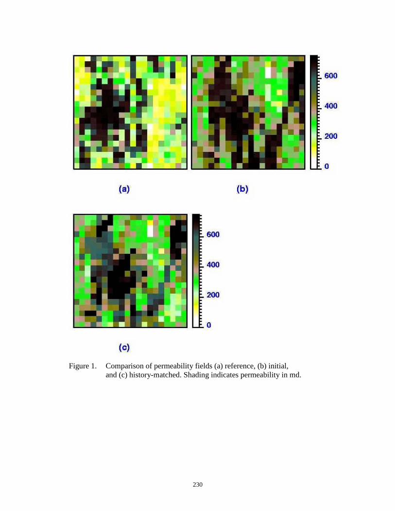
230

Figure 1. Comparison of permeability fields (a) reference, (b) initial, and (c) history-matched. Shading indicates permeability in md.

231

0. 0

0. 1

0. 2

0. 3

0. 4

0. 5

0. 6

0. 7

0. 8

0. 9

1. 0

0. 0 0. 2 0. 4 0. 6 0. 8 1. 0 1. 2 1. 4tD

fw

reference

ini tia l

inferred

Figure 2. Fractional flow curves for test case.

The example applications show that this approach is robust within the stated limitationsand converges quickly. Each iteration significantly reduces the errors in fractional flow, pressuredrop, and flow rate. In all of the examples, an acceptable match to the production data is obtainedwithin a small number of iterations. One strength of this approach is that the input of the inverseproblem is simply the usual output of the streamline simulation. Namely, streamline coordinates,production data including fractional flow, flow rate, and pressure. Therefore, this approach standsalone. Importantly, it appears to be expandable to integrate geostatistical data or to honorgeological and seismic data. We are actively pursuing this task and discuss this topic below.

Another strength is that repeated inversion of a matrix is not needed for the cases studied.The permeability modification for every iteration is computed directly based on differencesbetween the streamline breakthrough time from field observation and the simulation result.Therefore, this process takes very little computational time. All of the examples illustrated hereused the simplified inverse approach derived for unit mobility ratio cases. It appears that this ideaworks well for flow with unfavorable mobility ratios in heterogeneous reservoirs. Further studyis required.

232

Figure 3. Pressure history for test case.

The computation of the error in water-cut for both unit and non-unit mobility ratio cases isperformed using fractional-flow curves from the simulation and the reference results. The porevolume associated with each streamline is calculated for the purpose of sorting streamlines. Theaccuracy of computing streamline pore volume does not affect inversion results as long as thecorrect ordering of the breakthrough time is obtained. Therefore, for non-constant, non-unitmobility ratio cases, the method works well as long as the order of streamline breakthrough timeis preserved, even though the streamlines evolve.

Streamline permeability modifications are mapped directly to grid-blocks by propagatingthe indicated change through all of the grid-blocks that a particular streamline passes. Forexample, when the effective permeability of a streamline needs to be increased by 5 percent, thenthe permeability of all the grid-blocks along that streamline are increased by 5%. Mapping is notunique and different mapping schemes can produce the same effective streamline permeability.Necessarily, however, the water-cut curve is matched and the inferred field can be used to predictresults of other mobility ratios. In the mapping process, it is possible to enforce constraints tohonor observed geological information, if any.

Inverse solutions can be constrained in many different ways. Three approaches, asdescribed below, appear to be consistent with this approach.

0

1000

2000

3000

4000

5000

6000

7000

0. 0 0. 2 0. 4 0. 6 0. 8 1. 0 1. 2 1. 4tD

p

kPa

reference

ini tia l

infer red

233

A simple, but probably inefficient, method is to generate a number of permeability fieldsby sequential Gaussian simulation based on available geological information, and to checkwhether the effective permeability distribution from a particular realization matches that from theinversion. The check can be performed in the following way. Solve the pressure field and thestreamline distribution once for permeability field from geostatistical simulation. A unit mobilityratio should suffice. Sort the streamlines in the order of breakthrough time as we did for theinverse process. Compute the effective permeability and time of flight of each streamline,compare it with the effective permeability and time of flight from the inversion. In this manner,realizations are sorted. Those realizations within an acceptable value of the error in permeabilityare expected to generate a good match in production response, and therefore are accepted. It iseasy to generate geostatistical realizations and solve the pressure field once to obtain streamlinedistribution. This approach requires much less computational work than running a full flowsimulation on each realization.

Another way to constrain the inversion is to obtain a map of the expected pattern of highsand lows in the permeability field based on geological or seismic information The high and lowvalues would only be relative. When mapping the permeability modification from streamlines togrid-blocks, the decision of whether to modify the permeability of a grid-block could be based onwhether the permeability is to be increased or decreased, and whether this change agrees with thegeological information. Thus, permeability could be mapped to honor prior information about thefield.

A third approach is a combination of this work with the master-point idea (Wen et al.,1998).. We could compute the modification of the average permeability, and convert thismodification to a number of pre-selected master points (i.e, grid-blocks). Kriging is performed topropagate the modification at the master points to other grid-blocks. When kriging, weincorporate known geological information, such as direction of continuity and correlation length,and all the grid-blocks are reached for modification.

Examples shown here are for two-dimensional flow problems. We continue to work onthe generalization to three-dimensional problems with gravity. Additionally, this approach wasoriginally designed for incompressible two-phase flow or tracer flow studies. That is, thefractional flow curve or tracer breakthrough curve at the producers is required to infer theheterogeneity of the reservoir. More study is needed to extend this procedure to compressiblesingle-phase flow scenarios such as well test problems. Also, streamline simulation encountersdifficulties when infill wells are drilled, injectors are converted to producers, or vice versa, wellcompletions are changed, or radical changes are made in pattern balancing. In forward flowsimulation, such actions require that streamlines be recomputed. In history matching, multiplerealizations of streamline geometry would have to be honored. This is an important topic, but wemust address it later.

Results, indicate that the inverse solutions are very sensitive to relative permeability. It isnecessary to obtain accurate relative permeability curves in order to retrieve a good inversesolution. This is true of most history-matching approaches. As long as we use the same relativepermeability curves in both the forward simulation and inverse process, the inferred permeabilityfield will give us a good history match.

234

Actual production data is never as smooth as that in our synthetic examples. In general,for continuous injection of one phase to displace another phase, the fractional flow of the injectedphase at the producers is monotonically increasing. However, noise may cause it, apparently, notto be so. In such cases, we need to preprocess the data. The first step would be to usedimensionless time (pore volume) rather than real time. To reduce the effect of noise, a filter toremove small time scale variations (high frequency) is needed, while maintaining the variationsin large time scale. Normally, noise is random and therefore does not have a large time scaletrend. In general, it is the bulk reservoir properties that are important for predicting reservoirperformance, and they are represented in large time scale variations. Therefore, removing smalltime scale variation, even if it is not caused by noise, has small effect for prediction.

Conclusions

This approach relates producer water-cut curves to the breakthrough time of individualstreamlines. The effective permeability along streamlines is modified directly to history-matchthe fractional flow curve, pressure drop, and flow rate information. No matrix inversion isinvolved in the inverse process and therefore it is quite fast. The forward flow simulation with3DSL is also fast and so, for the examples examined, the entire process appears to becomputationally efficient.

The current work examined 2-D areal porous media, where the effect of gravity is notimportant, as well as incompressible two-phase flow. As with most history-matching approaches,high-quality noise-free data is needed for fast and accurate inversion. This approach works wellfor reservoirs where heterogeneity is a dominant factor. It also works well for unfavorablemobility ratios because the effects of heterogeneity are exacerbated by the unstable displacement.Although streamlines evolve for non-unit mobility ratio cases during the displacement process,we find it feasible to choose one streamline distribution and apply the simplified inverse systemduring the inversion.

Importantly, a permeability field inferred by matching production data for one mobilityratio can be used to predict reservoir performance for displacement processes at other mobilityratios.

Nomenclature

A cross-sectional area of a streamtube, L2

c constantE Absolute errore Relative errorfw fractional flow of waterk permeability, L2

krw relative permeability of waterkro relative permeability of oill streamline length

235

M mobility ratiop pressure, M/(Lt2)q flow rate, L3/ttD dimensionless timeV pore volume, L3

VP pore volumeVD ratio of pore volumexD dimensionless length

φ porosity

Subscripts:n producer indexi, j, k streamline indexsl streamlineBT breakthroughD dimensionless

Superscripts:C ComputedR Referenceλ iteration index

References

Batycky, R. P., Blunt, M. J., and Thiele, M. R.: “A 3D Field-Scale Streamline-Based ReservoirSimulator,” SPERE (November 1997) 246-254.

Blunt, M.J., Liu, K., and Thiele, M.R.:"A Generalized Streamline Method to Predict ReservoirFlow," Petroleum Geoscience (1996) 2, 259-269.

Brigham, W.E. and Abbaszadeh-Dehghani, M., "Tracer Testing for Reservoir Description," JPT(May 1987) 519-527.

Chu, L., Reynolds, A. C. and Oliver, D. S.: "Computation of Sensitivity Coefficients forConditioning the Permeability Field to Well-Test Pressure Data," In Situ , (1995) 19(2),179-223.

Deutsch, C. V. and Journel, A. G., GSLIB, Geostatistical Software Library and User’s Guide,Second Edition, Oxford University Press, New York (1998).

Dykstra, H. and Parsons, R.L., “The Prediction of Oil Recovery by Waterflood,” SecondaryRecovery of Oil in the United States, Principles and Practice, 2d ed., AmericanPetroleum Institute (1950), 160-174.

236

Fay, C. H. and Prats, M.. "The Application of Numerical Methods to Cycling and FloodingProblems" Proceedings of the 3rd World Petroleum Congress (1951).

Grinestaff, G.H.: "Waterflood Pattern Allocations: Quantifying the Injector to ProducerRelationship with Streamline Simulation," paper SPE 54616 presented at the 1999Western Regional Meeting, Anchorage, Alaska, 26-28 May.

Gupta, A. D., Vasco, D. W. and Long J.C.S.: “Detailed Characterization of Fractured LimestoneFormation Using Stochastic Inverse Approaches,” SPE Ninth Symposium (1994).

Hewett, T.A. and Behrens, R.A.: "Scaling Laws in reservoir Simulation and Their Use in aHybrid Finite Difference/Streamtube Approach to Simulation the Effects of PermeabilityHeterogeneity," in Reservoir Characterization, II, L. Lake and H.B.J. Carroll (eds.),Academic Press Inc., London (1991) 402-441.

Hewett, T. A., and Yamada, T.: "Theory of the Semi-Analytical Calculation of Oil Recovery andEffective Permeabilities Using Streamlines," Advances in Water Resources (1997) 20(5-6), 279-295.

Higgins, R.V., Boley, D.W. and Leighton, A.J.: "Aids to Forecasting the Performance of WaterFloods," JPT (September 1964) 1076-1082.

Higgins, R.V. and Leighton, A.J.: "A Computer Method to Calculate Two-Phase Flow in AnyIrregularly Bounded Porous Medium," JPT (June 1962) 679-683.

King, M.J., and Datta-Gupta, A.: "Streamline Simulation: A Current Perspective," In Situ, 22(1),(1998) 91-140.

Lake. L. W., Enhanced Oil Recovery, Prentice Hall, Englewood Cliffs, NJ (1989).

Landa, J. L. and Horne, R. N.: “A Procedure to Integrate Well Test Data, Reservoir PerformanceHistory and 4-D Seismic Information,” paper SPE 38653 presented at 1997 AnnualTechnical Conference and Exhibition in San Antonio, Texas, 5-8 October.

Lepine, O. J., Bissell, R. C., Aanonsen, S. I., Pallister, I. and W Barker, J.: "Uncertainty Analysisin Predictive Reservoir Simulation Using Gradient Information," SPE 48997, proceedingsof the SPE Annual Meeting, New Orleans (September 1998).

Martin, J.C. and Wegner, R.E.: "Numerical Solution of Multiphase, Two-DimensionalIncompressible Flow Using Streamtube Relationships," SPEJ (October 1979) 313-323.

Peddibhotla, S., Datta-Gupta, A., and Xue, G.: "Multiphase Streamline Modeling in ThreeDimensions: Further Generalizations and a Field Application," paper SPE 38003presented at 1997 Reservoir Simulation Symposium in Dallas, Texas, 8-11 June.

237

Portella, R. C. M. and Hewett, T. A.: "Fast 3-D Reservoir Simulation and Applications UsingStreamlines," paper SPE 39061 presented at the Fifth Latin American and CaribbeanPetroleum Engineering Conference and Exhibition in Rio de Janeiro, Brazil, 30 August-3September 1997.

Rahon, D., Edoa, P. F. and Masmoudi, M.: "Identification of geological shapes in reservoirengineering by history matching production data," SPE 48969, proceedings of the SPEAnnual Meeting, New Orleans (September 1998).

Thiele, M. R., Batycky, R. P., Blunt, M. J. and Orr Jr, F. M.Jr. “Simulating Flow inHeterogeneous Systems Using Streamtubes and Streamlines,” SPERE (February 1996) 5-12.

Thiele, M.R., Blunt, M.J., and Orr, F.M. Jr.: "Modeling Flow in Heterogeneous Media UsingStreamtubes--I. Miscible and Immiscible Displacements," In Situ (August 1995) 19(3),299-339.

Thiele, M.R., Blunt, M.J., and Orr, F.M. Jr.: "Modeling Flow in Heterogeneous Media UsingStreamtubes--II. Compositional Displacements," In Situ (1995) 19(4), 367-391.

Vasco, D.W. and Datta-Gupta, A.: "Integrating Multiphase Production History in StochasticReservoir Characterization," SPEFE (September 1997) 149-156.

Vasco, D.W., Yoon, S. and Datta-Gupta, A.: “Integrating Dynamic Data Into High- ResolutionReservoir Models Using Streamline-Based Analytic Sensitivity Coefficients,” paper SPE49002 presented at 1998 Annual Technical Conference and Exhibition in New Orleans,Louisiana, 27-30 September.

Wang, Y.D., Kovscek, A. R. and Brigham, W.E.: “Effect of Mobility Ratio on Pattern Behaviorof a Homogeneous Porous Media”, In-Situ, 23(1) (1999) 1-20.

Wen, X.H., Clayton, D.V. and Cullick A.S.: “High Resolution Reservoir Models IntegratingMultiple-Well Production Data,” SPEJ (December 1998) 344-355.

Wen, X.H., Clayton, D.V. and Cullick A.S.: "Integrating Pressure and Fractional Flow Data inReservoir Modeling with Fast Streamline-Based Inverse Method," paper SPE 48971presented at 1998 Annual Technical Conference and Exhibition in New Orlean,Louisiana, 27-30 September.

Wu, Z., Reynolds, A. C. and Oliver, D. S.: "Conditioning Geostatistical Models to Two-PhaseProduction Data," SPEJ (June 1998) 142-155.

238

History Matching Constrained to Geostatistical Data

(Task 5)

Introduction

Geostatistical techniques are used primarily to generate realistic equally probablenumerical reservoir models that honor known geological information. However, significantuncertainty exists in the detailed distribution of reservoir properties such as permeability(Deutsch and Srinivasan, 1996) because the known data is relatively sparse. If flow simulation isperformed on various realizations to predict reservoir performance, geological reservoir modeluncertainty is transferred into a relatively uncertain prediction of future production.

The reliability of geostatistical reservoir models as applied to flow simulation increases asdynamic data, such as production history, is incorporated (cf. Tran et al. 2001). However,integration of production history with geostatistical information is, to date, computationally timeconsuming. The problem is generally approached through inverse modeling where a constrainedoptimization problem is solved. That is, dynamic data, such as oil production rate, water cut, orpressure, are matched by adjusting parameters within a subspace of parameter values. Inversion isboth CPU demanding and poorly determined because the number of parameters adjusted is large.For instance, a problem might be constructed where the permeability of every gridblock in areservoir model is treated as an unknown.

The history-matched models (or inverse solutions) can be constrained to geology in manydifferent ways. The following two approaches appear to be consistent with our streamline-basedinverse method: (1) incorporating geostatistical constraint directly into our history-matchingprocess; and (2) streamline time-of-flight ranking of reservoir models. First we focuse on theintegration of a geostatistical technique called Gauss-Markov random functions with thestreamline inverse method. The streamline approach is then summarized.

Gauss-Markov Random Functions (GMrf)

The GMrf technique is similar to sequential Gaussian Simulation (SGSIM) (Deutsch andJournel, 1998). GMrf uses a Markov chain Monte Carlo method to constrain realizations suchthat they honor a specific variogram and histogram (Caers, 2001). The main difference betweenGMrf and SGSIM is that GMrf is iterative, while SGSIM is a non-iterative technique. SGSIMstarts with an empty grid and then simulates that grid sequentially node by node along a randompath. The procedure finishes when every node is simulated. The problems with SGSIM are that itis difficult to constrain the realizations to complex data types, and that only linear constraints arepermitted. GMrf has the same goal as SGSIM, i.e., generating realizations with a specificvariogram and histogram. The procedure operates node by node, changing the value at each nodeaccording to a probabilistic criterion. When the procedure iterates long enough, both thevariogram and the histogram will be honored. The key is how to choose the probabilisticcriterion, which is based on a new geostatistical idea that seems similar to the simulated

239

annealing technique. The method is faster than simulated annealing, there is no objectivefunction criterion, and we need not set any cooling schedule (Caers, 2001).

The fact that the grid is “full” while iterating, as opposed to SGSIM where the grid isfilled gradually, allows us to condition the model to much richer data. Caers (2001) has extendedthis technique to include any type of nonlinear, multiple-point averaging constraints. In ourapplications, the constraint is the effective permeability of relevant streamlines. The inverse resulthonors the production history with effective permeabilities along streamlines, but not necessarilythe variogram and/or histogram. So, the GMrf technique is used to post-process the inverse resultat every iteration and turn it into a realization that honors the variogram/histogram, effectivepermeabilities, and the production data.

Integration of GMrf into Streamline-Based History-Matching

There are different ways to combine GMrf and our streamline inverse method such thatthe resulting models honor both the geology and production history. The following two ways aremost appropriate. The first is to integrate GMrf and our inverse method in the true sense. In thisapproach, we solve the history-matching and GMrf problem simultaneously, i.e., performing theinverse process and GMrf as a whole in each iteration. The second approach is to perform thetwo processes sequentially. That is, in each iteration, we first perform the streamline-basedinverse process, which may destroy the geological consistency slightly. Then, we run the GMrfprocess as a remedy to restore the correct geology into the history-matched models.

Both approaches have advantages and disadvantages. In the first approach, the twoprocesses are tightly coupled. The modification of the model parameters in each iteration honorsboth geology and production history; therefore, its rate of convergence is expected to be higherthan that of the second approach. However, due to the coupling, the implementation can be morecomplicated. In the second approach, the two processes run independently, with GMrf followingthe streamline inverse process. The two procedures are decoupled; therefore, they can bedeveloped separately and are applied together to achieve our goal. Because we have developedthe algorithm and computer programs for the two methods, we can readily combine the twoexisting parts to construct the new method. However, because the two procedures are not trulyintegrated, the negative effect of one process on the other cannot be eliminated by designing newalgorithm and code. Consequently, the convergence rate may suffer.

We implemented the second approach. However, the two components still need minormodification to accommodate each other. For example, the streamline inverse method needs tobe modified to output necessary information used in the GMrf process, including streamlinecoordinates, time-of-flight, and effective permeability. The GMrf code also needs to be modifiedso that the streamline effective permeability is honored.

Moreover, we try to minimize the negative effect of one component on the other. Thestreamline history-matching method may introduce streamline-related artifacts in the permeabilityfield. If we modify the permeability field as required by the inverse process in each iteration, itmay cause an excessive number of iterations within the GMrf process to restore the correct

240

variogram and histogram. To reduce the GMrf cost, we introduce a dampening (or decelerating)factor η < 1 in the calculation of the streamline effective permeability modification:

kiλ+1 = ki

λ (1 + ηδiλ+1) (1)

where the superscripts and subscripts are the indices of iterations and streamlines, respectively; kis the streamline effective permeability; and δ is the relative change of k.

On the other hand, if we choose a value of η that is too small, we need more historymatching iterations; consequently increasing the cost of the entire method. By our investigation,an optimal η range is from 0.2 to 0.7. We may use large values during initial iterations and smallvalues in iterations near the end of the history-matching.

Algorithm

As stated above, we use the second approach to combine the GMrf technique with ourstreamline inverse process, i.e., performing history-matching and GMrf sequentially. Theprocedure is summarized as follows:

1. Choose an initial reservoir model. It is beneficial to have an initial model that honors theknown or assumed geology so that less computation occurs in the GMrf process. We useSGSIM to generate the initial reservoir model (expressed as a permeability distribution in ourcase study).

2. Perform the history-matching procedure as described in Chapter 3 to obtain: (1) thepermeability value k(u) for each grid-block/location u; (2) the geometry and time-of-flight ofeach streamline; and (3) the effective permeability of each streamline. After this inverseprocess, the match to the production data is improved, but the resulting model may violate thegeology as expressed by the variogram and histogram in the permeability distribution.

3. Use the GMrf procedure (Caers, 2001) that takes the model obtained in Step 2 as its initialreservoir model and “superpose” the variogram on it using an iterative procedure as follows:

4. Transform the permeability values k(u) to the standard normal space to obtain y(u);

5. Traverse iteratively through the normal space grid. For each visited grid block uijk, propose anew value ynew(uijk) drawn from the marginal distribution, transform it into the data spaceknew(uijk) and then accept it with the Metropolis sampling probability;

6. Continue iterations until convergence of GMrf.

7. Check the match to the historic production data. Iterate Steps 2 and 3 until a satisfactorymatch to production history is achieved.

241

In the GMrf procedure (Step 3), the distribution of permeability values in the domain ismade to honor the variogram and histogram. The effective permeability along each streamline isnot changed. The effective permeability of a streamline is the time-of-flight weighted harmonicaverage of permeability values of all the grid-blocks the streamline passes. When proposing amodification, we use the geometry, time-of-flight and effective permeability of streamlinesobtained in Step 2 so that the effective permeability of all streamlines are honored. By doing so,we assume the streamline geometry does not evolve radically as a result of this post processing.

To generate multiple geostatistical realizations, we perform the method with a differentrandom seed each time. We can also perform the inverse process with a different initialgeostatistical model from which our final inverse result will most likely have different streamlinegeometry. Using the multiple realizations that honor geology and production history, we quantifythe degree of uncertainty in the prediction of future reservoir performance.

Results and Discussion -- GMrf

Four example applications are presented below. First, a simple five-spot pattern case withisotropic permeability distribution and unit mobility ratio demonstrates the working of thismethod. Next, a similar case shows this method works equally well for a nonunit mobility ratiocase (M= 2.5). Then, a case with an anisotropic field was studied. In the last case, our methodwas used to match a short production history and then we examine the prediction of reservoirperformance using the history-matched models. Throughout this section, we used the GSLIBprogram SGSIM (Deutsch & Journel, 1998) to generate permeability models, and the streamlinesimulator 3DSL (Batycky et al., 1997) to perform forward flow simulation. In each example, ourmethod worked effectively and generated reservoir models that honor both geology and historicproduction data.

Cases 1: Five-spot, Isotropic Permeability Field, M=1

We use this simple case to demonstrate the method. The case scenario is as follows:100x100 grid-block isotropic permeability field, five-spot pattern with the injector in the centerand four producers in the four corners. Water is injected at a constant rate and the pressure isfixed at the producers. First, we generate a reference permeability field; its distribution,histogram and variogram are shown in Fig. 1. Flow simulation is run on this permeability field toobtain the reference production history. Some parameters to run the flow simulation are given inTable 1. Unit mobility ratio is used. Another permeability field is generated and used as theinitial model. In the inverse process, 178 streamlines are launched; an η value of 0.3 is used forall iterations.

Nine iterations were performed to obtain an acceptable match to the production data.Figure 2 shows the gradual change of permeability distribution of iteration 1, 2, 5 and 9. The leftcolumn figures are prior to the GMrf constraining process, while the right are after the GMrfprocess, and therefore, consistent with geology. The permeability fields in the left column,though not visually obvious, do not satisfactorily describe the known geology. Figure 3 shows

242

the final history-matched realization, its histogram and variogram. Figure 4 shows the match tothe water-cut at all four producers. The match is acceptable.

Table 1 Summary of Flow Simulation Parameters for the Four Cases

Pattern Grid M PV qinj Sor Swc0rwk 0

rok kr wµ oµ(m3) (m3/day) eqns (cp) (cp)

CCase 1

100x100 1 100000 300 0 0 1.0 1.0Set 1

1 1

Case 2 100x100 2.5 100000 300 0.2 0.2 0.2 0.2 Set 2 1 10Case 3 200x200 1 100000 300 0 0 0 0 Set 1 1 1Case 4 100x100 5 100000 300 0.2 0.2 0.2 0.2 Set 2 1 20

Set 1: k rw = krw0 ( sw − s wc ), k ro = k ro

0 (s o − s ro )

Set 2: k rw = krw0 s w − s wc

1 − sor − s wc

2

, kro = kro0 1 − sor − sw

1 − s or − swc

2

Cases 2: Five-spot, Isotropic Permeability Field, M=2.5

We also studied an unfavorable mobility ratio case in which water displaces oil. We usethe same reference and initial permeability field and same well configuration as in the unitmobility ratio (tracer) case above, but change the fluid properties (see Table 1), resulting an end-point mobility ratio of 2.5. During history-matching, the dampening factor used and the numberof streamlines launched are the same as in the previous case.

The history-matching took eight iterations, which is smaller than in the unit mobility ratiocase, to obtain an acceptable match to the production history. However, each iteration requiredmore computation than that in the previous case, because we need to solve the pressure field morefrequently to obtain an accurate flow simulation result.

Figure 5 shows the final history-matched permeability field, its histogram and variogram.Figure 6 shows the match to the water-cut history. The match is acceptable in terms of bothgeology and production history; though the final permeability field is different from that of theprevious case. The result indicates our method works equally well for non-unit mobility ratiocases.

243

Figure 1. Reference permeability field, histogram and variogram, 100x100.

244

Figure 2. Permeability field at iterations 1, 2, 5 and 9. The left column is prior to the GMrfprocess, while the right is after the GMrf and therefore consistent with geology.

245

Figure 3. History-matched permeability field (100x100), five-spot, M=1.

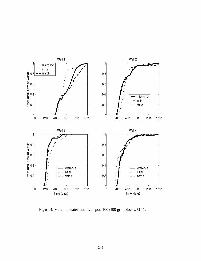
246

Figure 4. Match in water-cut, five-spot, 100x100 grid-blocks, M=1.

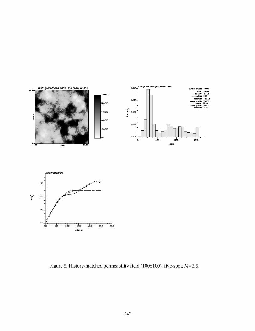
247

Figure 5. History-matched permeability field (100x100), five-spot, M=2.5.

248

Figure 6. Match in water-cut, five-spot, 100x100 grid-blocks , M=2.5.

249

Cases 3: Five-spot, Anisotropic Permeability Fields

We used SGSIM to generate the reference and initial permeability fields with the majordirection of continuity set to N45W. There are 200x200 grid-blocks. Figure 7 shows thereference permeability field, its histogram and variogram. The same well locations and fluidproperties as in the previous case are used to run the flow simulation. The key parameters used inthe flow simulation are given in Table 1. A dampening factor of 0.25 was used; about 300streamlines are launched in the inverse process.

Eight iterations were used to obtain a satisfactory history-match. Figures 8 and 9 showthe history-matched realization and the match to water-cuts of all four producers. The match tothe production history and the reproduction of the variogram and histogram are excellent. It tookabout three hours to history-match this 40,000 grid-block model and the major computational costis for the eight runs of the streamline simulator (Table 2).

Cases 4: Prediction of Reservoir Performance Using the History-Matched Model M=5

In this case, we demonstrate how our method is used to obtain a reservoir model thatmatches a short period of production history; then, the model is used to predict the futurereservoir performance, including water-cut and cumulative oil production. We use SGSIM togenerate reference (Fig. 10) and initial permeability fields, and use 3DSL to create referencereservoir performance. Simulation parameters are listed in Table 1. Next, starting from an initialmodel, we perform the above history-matching process to match only an initial portion of thereference. Then, the history-matched model is used to run flow simulation and compare with therest of the reference performance.

Starting from an initial permeability field, we performed the history-matching process three timeswith different random paths. Seven to eight iterations were used to obtain an acceptable match tothe partial production history—150 days or 0.75 PVI. The three history-matched models areshown in Fig. 10. The matches and predictions of water-cut are shown in Fig. 11; the matchesand predictions of cumulative oil production are given in Fig. 12. Compared with the initialmodel, which does not reproduce the reference results, the history-matched models producedexcellent matches to the reference in terms of both the historic and the future performance.

250

Figure 7. Reference permeability field, histogram and variogram, 200x200 grid-blocks.

251

Figure 8. History-matched permeability field (200x200 grid-blocks), five-spot, M=1.

252

Figure 9. Match in water-cut, five-spot, 200x200 gridblocks, M=1.

253

Figure 10. Reference and history-matched permeability fields.

254

Figure 11. Match and prediction of water-cut. Matched to a production historyof 150 days. The rest is prediction.

255

Figure 12. Match and prediction of cumulative oil production. Matchedto a production history of 0.75 PVI. The rest is prediction.

256

Computational Cost

Table 2 shows the overall computational work for each case and its breakdown for eachcomponent of the inverse process. The jobs were run on a 600 MHz DEC alpha machine.For a small number of grid-blocks (50 by 50 case) and unit mobility ratio, the major cost can beattributed to GMrf. This is largely due to the computing overhead associated with the GMrf.However, as the number of grid-blocks increases, the computational work of the flow simulationincreases rapidly, while that of GMrf procedure increases at slower rate. We observed that theCPU cost of the flow simulation grows quadratically with the number of grid-blocks, while thatof the GMrf process grows slightly faster than linearly. Computational work by the streamlineinverse process also scales linearly with the number of grid-blocks. In any case, the CPU timeconsumed by the streamline inverse process is negligible when compared with the other two parts(GMrf and forward simulation).

For nonunit mobility ratios, the pressure field and streamline geometry must be updatedperiodically during forward simulation to obtain accurate results. Hence, the CPU-time issomewhat greater for the M=2.5 and M=5 cases, as compared to the M=1 cases.

Table 2 Computational Work

Case Case CPU per iteration (sec) # Total CPU# Description 3dsl GMrf SLInv Total

Iterations(sec) (min)

1 5-spot, 100x100, M=1 76 69 1.4 146 9 1318 22.02 5-spot, 100x100, M=2.5* 1169 69 1.4 1239 8 9915 165.33 5-spot, 200x200, M=1 1285 338 6.0 1629 8 13032 217.24 5-spot, 100x100, M=5* 1254 69 1.4 1324 7~8 9933 165.6

*--Non-unit mobility ratio, more pressure solves required than M=1 case.

Remarks

We propose a combined streamline-geostatistical history matching procedure. Themethodology relies on decoupling of the inversion process to the greatest extent possible. Flowhistory and geology are matched in a two-step procedure: a streamline method calculates adesired change in streamline effective permeabilities and a geostatistical routine spreads thisdesired change to account for known geological variations.

No matrix inversion is necessary in the streamline inversion portion, the Gauss-Markovtechnique is an efficient optimization algorithm, and forward simulation is conducted with astreamline simulator. Hence, the methodology is fast, and the major computational cost is theforward flow simulation. However, the combined geostatistical and streamline-based methodshares many of the advantages and limitations of its two basic components. The limitations ofstreamline inverse methods have been discussed in the previous section.

257

Inverse solutions can be constrained in many different ways. One of the main advantagesof the proposed technique lies in the decoupling of the streamline-based inversion from thegeostatistical simulation algorithm. In a sense, the effective permeability along streamlinesrequired to match production data is computed without any knowledge of geology. Geostatisticsis then used to distribute grid-block permeability in a consistent manner that restores geology.However, since the harmonic averages in Step 2 of the algorithm are calculated withoutknowledge of the underlying histogram and variogram model, inconsistencies can occur betweenStep 2 and Step 3 of the algorithm. Therefore, the introduction of a dampening factor is crucial tomake the combined procedure of history-matching and GMrf robust and efficient. Essentially,the dampening factor limits the degree of change and prevents overly drastic permeabilitymodification that may introduce difficulty in convergence of the GMrf process.

All the example applications show acceptable matches to the production history andreproduction of variogram and histogram within a few iterations. Our method works equally wellfor cases with unit and non-unit mobility ratios. Importantly, if a short period of productionhistory is matched using our method, the uncertainty of the model can be substantially reducedwhile the model is used to forecast the future reservoir performance, as opposed by using ageostatistical reservoir model that has not been history-matched.

The current methodology allows only for quantification of geology in terms of avariogram, yet the decoupled procedure could lead to an extension of the algorithm to account forother types of geological models (e.g., channels). More study is needed to pursue this concept.

Streamline-Based Ranking

To address jointly production history and constraint to a prior geological model, we alsohave proposed and demonstrated ranking suites of reservoir models in terms of streamlineproperties. A subset is then selected rationally that honor observed production data. The rankingapproach is somewhat similar to importance sampling (Barker et al. 2001), but requiressubstantially less computation to evaluate the objective function. Additionally, results are lesssensitive to the prior reservoir model. In streamline ranking, the objective function measures themismatch of streamline properties between any given and a desired (i.e., reference) reservoirmodel. The mismatch is evaluated efficiently by calculating, for instance, the distribution of theTOF of streamlines reaching a producer. By sampling a sufficient number of reservoir models, aset of models that honor desired streamline properties are identified. It has been demonstrated thatranking according to TOF also sorts models in regard to historic production data, such as water-cut. The use of full flow simulation in minimized throughout the algorithm.

Results from this study have been published already (Wang and Kovscek 2002, 2003). Byway of summary, the work proceeded by first providing the empirical observations and limitedtheoretical development that form the background for streamline ranking. We established thecorrelation among streamline properties and the corresponding comprehensive flow simulationresults. The algorithm arising by the correspondence of streamline and flow simulation resultswas then described. Synthetic examples illustrate application of the method under various

258

conditions. A brief digression showed that streamline ranking can be employed for downscalingconsistently coarse-grid history-matched reservoir models.

Method

The ranking method is summarized in the following. The major assumptions include 1)the history of injected phase production is available; 2) no drastic changes of well conditions(e.g., shut in or in fill); and 3) gravity, capillary forces, and compressibility are not important.

The ranking procedure:1. Start from an initial reservoir model and perform history matching (Wang and Kovscek,

2000) to obtain a history-matched reservoir model that is not necessarily constrained togeology. For unit mobility ratio, the water-cut curve is the same as the streamline TOF cdf asshown above. In this case, the reference water-cut curve is used directly as the referencestreamline TOF cdf.

2. For the history-matched model and each of the models to be ranked, compute the pressuredistribution for unit mobility ratio, streamline geometries, and streamline TOF cdf for eachproducer. Pollock’s (1998) method is used here to compute streamline geometries.

3. For each of the reservoir models to be ranked, compute the mismatch of its streamlineproperties, such as TOF cdf, q, and E

pN , with respect to the history-matched model. This

computation is performed for each producer.

4. Rank the reservoir models based on the mismatch type of interest. For instance, if a match ofthe water-cut is desired, then streamline TOF cdf ranking should be used.

5. Select a suitable number of models within a specified tolerance and perform comprehensiveflow simulation to evaluate the match in simulation results, predict future reservoirperformance, as well as quantify the uncertainty of the prediction.

Conclusions

A method is proposed to rank rapidly reservoir models. This method is based on theobservation that there is approximately a linear correlation between unit mobility ratio streamlineproperties and nonunit mobility ratio reservoir flow simulation results, under appropriateassumptions. The streamline time-of-flight cumulative distribution function indicates theconnectivity between injector-producer pairs, and consequently it is characteristic of flowsimulation results regardless of mobility ratio. Exhaustive flow simulation and theoreticalderivation established correlation among the following data pairs: 1) streamline TOF cdf andproducer water cut, 2) unit mobility flow-rate at one time value and that in comprehensive flowsimulation, and 3) E

pN and pN . With these data pairs, reservoir models ranked in terms of

streamline properties are also ranked in terms of their match to the observed production history.

259

Computation of streamline geometries and properties is computationally efficient. Thecomputational effort per reservoir model is equivalent to one time-step of an IMPES flowsimulation.

The ranking method requires that a history-matched model be obtained first. The historymatch does not necessarily need to be constrained to geology. Then, geostatistically consistentmodels are generated and compared to the history-matched model with regard to streamlineproperties. A subset of models with tolerable mismatch are selected to run flow simulation andthereby verify that they match the observed behavior. In this manner, multiple models areobtained that reproduce satisfactorily production history and are constrained to geologicalinformation. An exercise demonstrated that partial production history when used in combinationwith streamline-based ranking reduced significantly the uncertainty of forecasting reservoirperformance.

The ranking results do not depend on the history-matching method or the initial reservoirmodel, but depend on the accuracy of the match used to obtain the target TOF cdf. Additionally,there is no restriction that the reservoir models must have the same grid-block dimensions as thehistory-matched model. Therefore, fine-grid models with a million cells can be ranked andselected efficiently when history matching is performed on a coarse grid. This provides anefficient way to downscale history-matched models.

References

Barker, J. W., Cuypers, M. & Holden, L. 2001. “Quantifying Uncertainty in ProductionForecasts: Another Look at the PUNQ-S3,” SPE Journal, 6(4) 433-441.

Batycky, R. P., Blunt, M. J. & Thiele, M. R. 1997. “A 3D Field-Scale Streamline-BasedReservoir Simulator,” SPE Reservoir Engineering, 12, November, 246-254.

Caers, J., Krishnan, S., Wang, Y. & Kovscek, A. R. 2002. “A Geostatistical Approach toStreamline-based History Matching” to appear SPE Journal.

Deutsch, C. V. & Journel, A. G. 1998. GSLIB, Geostatistical Software Library and User’s Guide,Second Edition, Oxford University Press, New York.

Deutsch, C. V. & Srinivasan, S. 1996. “Improved Reservoir Management Through RankingStochastic Reservoir Models,” SPE 35411 presented at SPE/DOE tenth Symposium onImproved Oil Recovery, Tulsa, OK, 21-24 April, 105-112.

Tran, T. T, Wen, X-H., & Behrens, R. A. 2001. "Efficient Conditioning of 3D Fine-ScaleReservoir Model to Multiphase Production Data Using Streamline-Based Coarse-ScaleInversion and Geostatistical Downscaling", SPE Journal, 6(4), 364-374.

Wang, Y. and A. R. Kovscek, "Integrating Production History into Reservoir Models UsingStreamline-Based Time-of-Flight Ranking," Petroleum Geoscience, 9(2), 163-174 (2003).

260

Wang, Y. and A. R. Kovscek. "A Streamline Approach for Ranking Reservoir Models thatIncorporates Production History" SPE 77377, Proceedings of the SPE Annual TechnicalConference and Exhibition, San Antonio, TX, Sept. 29 - Oct. 2, 2002.

261

Area 6. Technology Transfer

Technology transfer was an important part of our research efforts. It wasconsidered so important that it was made an explicit part of the work plan and becameArea 6. Technology transfer was accomplished through a variety of venues including:

• an annual industrial review meeting

• technical presentations at appropriate symposia, technical meetings, and workshops

• publication of technical papers, reviews, and chapters for the Society of PetroleumEngineers Handbook

• training of students who are subsequently hired by the domestic oil industry

• creation of a world wide web site (http://ekofisk.stanford.edu/supria.html)

• a short course on thermal recovery for practicing engineers

• international cooperation

Because all of our work is in the public domain, we aim for significant, rapid, andbroad dissemination of our research results. Further discussion of our technology transferefforts in each area follow.

Industrial Review Meeting

We host a review meeting annually to review with industrial representatives ourcurrent research results and research in progress. This review provides industry with anopportunity to see our work first hand and provide a critique. Meetings consist oftechnical presentations followed by extensive question and answer periods. Tours of ourlaboratory and one-on-one meetings between industry and SUPRI personnel also occur.Some time is also alotted for open discussion.

During the period of performance meetings were held April 19-20, 2001, April18-19, 2002, and April 22-23, 2003. Attendees from D.O.E., Aera Energy LLC,ChevronTexaco, ConocoPhillips, ExxonMobil, PDVSA-Intevep, Shell,Total, TycoThermal Controls participated in the various meetings.

Technical Presentations

Presentation of research results at technical meetings and workshops was aprinciple means of technology transfer, in addition to the industrial review meetings.

http://ekofisk.stanford.edu/supria.html

262

Most of the presentations occurred at Society of Petroleum Engineers (SPE) meetings asthese meeting were judged to have the greatest audience with an interest in our research.The specific meetings attended to conduct technology transfer include: 6th InternationalSymposium on Evaluation of Reservoir Wettability and Its Affect on Oil Recovery(2000), SPE International Thermal Operations and Heavy Oil Symposium (2001), SPEWestern Regional Meetings (2001, 2002, 2003), SPE Annual Technical Conference andExhibition (2001, 2002, 2003), and the SPE/DOE Thirteenth Symposium on EnhancedOil Recovery (2002). A listing of authors and paper titles is given at the end of thissubsection under the heading “Conference Presentations”.

During the period of performance, we also participated with the West CoastPetroleum Technology Transfer Council during a workshop (2001) that they hosted. Thetopic during the workshop was a review of diatomite physical properties and theirrelation to hydraulic fracturing. A variety of people from companies operating in the SanJoaquin Valley attended. A variety of presentations were also made at the University ofCalifornia, Berkeley (2002, 2003), ChevronTexaco, and Aera Energy LLC (2003).

Conference Presentations

Arora, P. and A. R. Kovscek, “Mechanistic Modeling of Solution Gas Drive in ViscousOils, SPE 69717, Proceedings of the SPE International Thermal Operations andHeavy Oil Symposium, Porlamar, Venezuela March 12-14, 2001.

Hoffman, B. T. and A. R. Kovscek, “Light-Oil Steamdrive in Fractured LowPermeability Reservoirs,” SPE 83491, Proceedings of the SPE WesternRegion/AAPG Pacific Section Joint Meeting, Long Beach, CA, May 19-24, 2003.

Kovscek, A. R. and H. J. Bertin, "Estimation of Foam Mobility in Heterogeneous PorousMedia, " SPE 75181 Proceedings of the SPE/DOE Thirteenth Symposium onImproved Oil Recovery, Tulsa, OK April 13-17, 2002.

Rangel-German. E. R. and A. R. Kovscek, “Time-Dependent Matrix-Fracture ShapeFactors for Partially and Completely Immersed Fractures,” SPE 84411,Proceedings of the SPE Annual Technical Conference and Exhibition, Denver,CO, Oct. 5-8. 2003.

Rangel-German, E. R. and A. R. Kovscek, "Water Infiltration in Fractured Systems:Experiments and Analytical Model," SPE 71618 Proceedings of the SPE AnnualTechnical Conference and Exhibition, New Orleans, LA Sept. 30 - Oct. 3, 2001.

Ross, C. M. and A. R. Kovscek, "Pore Microstructure and Fluid Distribution in aDiatomaceous Reservoir, " SPE 75190 Proceedings of the SPE/DOE ThirteenthSymposium on Improved Oil Recovery, Tulsa, OK April 13-17, 2002

263

Schembre, J. M. and A. R. Kovscek, " Direct Measurement of Dynamic Relative Permeabilityfrom CT-Monitored Spontaneous Imbibition Experiments," SPE 71484 Proceedings of theSPE Annual Technical Conference and Exhibition, New Orleans, LA Sept. 30 - Oct. 3,2001.

Tang, G.Q. and A. R. Kovscek, "Experimental Study of Heavy Oil Production from DiatomiteCore at Elevated Temperatures, " SPE 75132 Proceedings of the SPE/DOE ThirteenthSymposium on Improved Oil Recovery, Tulsa, OK April 13-17, 2002.

Tang, G-Q. and A. R. Kovscek, "Wettability Alteration of Diatomite Induced by Hot-FluidInjection" SPE 77461, Proceedings of the SPE Annual Technical Conference andExhibition, San Antonio, TX, Sept. 29 - Oct. 2, 2002.

Tang, G.-Q., Y. Leung, L. M. Castanier, A. Sahni, F. Gadelle, M. Kumar, and A. R. Kovscek,“An Investigation of the Effect of Oil Composition on Heavy Oil Solution Gas Drive,”SPE 84197, Proceedings of the SPE Annual Technical Conference and Exhibition,Denver, CO, Oct. 5-8. 2003.

Wang, Y. and A. R. Kovscek. "A Streamline Approach for Ranking Reservoir Models thatIncorporates Production History" SPE 77377, Proceedings of the SPE Annual TechnicalConference and Exhibition, San Antonio, TX, Sept. 29 - Oct. 2, 2002.

Zhou, D., L. Jia, J. Kamath, and A. R. Kovscek, “Scaling of Counter-Current ImbibitionProcesses in Low-Permeability Porous Media,” Proceedings of the 6th InternationalSymposium on Evaluation of Reservoir Wettability and Its Effect on Oil Recovery,Soccoro, NM September 27-28, 2000.

Zhou, D., L. Jia, J. Kamath, and A. R. Kovscek, “An Investigation of Counter-Current ImbibitionProcesses in Diatomite,” SPE 68837, Proceedings of the SPE Western Regional Meeting,Bakersfield, CA March 26-30, 2001.

Technical Papers

To aid in the dissemination and documentation of technical results, a series of papers weresubmitted to journals. An advantage of the submission of work to journals is that papers aresubjected to anonymous peer review. Thus, a form of quality control is associated with publishedwork. A listing of authors and peer-reviewed manuscript titles is given at the end of thissubsection under the heading “Reviewed Manuscripts”.

A highlight of this aspect of our technology transfer efforts was the publication of achapter on in-situ combustion for the Reservoir Engineering Section of the Society of PetroleumEngineers Handbook (Castanier and Brigham, 2003). During past Industrial Review CommitteeMeetings, it was suggested rather strongly by attendees that while in-situ combustion has greatpotential as a thermal recovery technique, it is still viewed as a high-risk process by many. Theystated that we should clarify the potential of in-situ combustion as an enhanced oil recovery

264

process and try to capture some of the knowledge with regard to design aspects of ISC projects.An invitation from the Society of Petroleum Engineers to prepare a chapter for the latest versionof the Petroluem Engineers Handbook allowed this suggestion to take shape.

Reviewed Manuscripts

Apaydin, O. and A. R. Kovscek, "Surfactant Concentration and End Effects on Foam Flow inHomogeneous Porous Media," Transport in Porous Media, 43(3), 511-536 (2001).

Akin, S. and A. R. Kovscek, "Heavy Oil Solution Gas Drive: A Laboratory Study," Journal ofPetroleum Science and Engineering, 35(1-2), 33-48 (2002).

Arora, P. and A. R. Kovscek, “A Mechanistic Modeling and Experimental Study of Solution GasDrive,” Transport in Porous Media, 51, 237-265 (2003).

Bertin, H. J. and A. R. Kovscek, " Foam Mobility in Heterogeneous Porous Media I: ScalingConcepts," Transport in Porous Media, 52, 17-35 (2003).

Bertin, H. J. and A. R. Kovscek, " Foam Mobility in Heterogeneous Porous Media II:Experimental Observations," Transport in Porous Media, 52, 37-49 (2003).

Caers, J., S. Krishnan, Y. Wang, and A. R. Kovscek, "A Geostatistical Approach to Streamline-Based History Matching," Society of Petroleum Engineers Journal, 7(3) Sept, 250-266(2002).

Castanier, L. M. and W. E. Brigham, “In Situ Combustion” , Chapter 17, Reservoir EngineeringSection, Society of Petroleum Engineers Handbook, Richardson TX: Society of PetroleumEngineers, in press 2004.

Castanier, L. M. and W. E. Brigham, “Upgrading of Crude Oil Via In Situ Combustion,” Journalof Petroleum Science and Engineering, 39(1&2), 125-136 (2003).

Diabira, I., L. M. Castanier, and A. R. Kovscek, "Porosity and Permeability EvolutionAccompanying Hot Fluid Injection into Diatomite," Petroleum Science and Technology,19(9&10), 1167-1185 (2001).

Elliot, K. T. and A. R, Kovscek, “A Numerical Analysis of the Single-Well Steam AssistedGravity Drainage Process,” Petroleum Science and Technology, 19(7&8), 733-760(2001).

George, D. S., O. Hayat, and A. R. Kovscek, “A Microvisual Study of Solution Gas DriveMechanisms in Viscous Oils,” Journal of Petroleum Science and Engineering, in review,submitted March 2003.

265

Hoffman, B. T. and A. R. Kovscek, “Efficiency and Oil Recovery Mechanisms of SteamInjection into Low Permeability, Hydraulically Fractured Reservoirs,” Petroleum Scienceand Technology, to appear.

Kovscek, A. R. and C. J. Radke, “ Pressure-Driven Capillary Snap off of Gas Bubbles at LowWetting-Liquid Content”, Colloids and Surfaces A: Physicochemical and EngineeringAspects, 212(2&3), 99-108 (2003).

Tang, G.-Q. and A. R. Kovscek, “An Experimental Investigation of the Effect of Temperature onRecovery of Heavy Oil From Diatomite,” Society of Petroleum Engineers Journal, inreview, submitted January 2003.

Rangel-German, E. R. and A. R. Kovscek,"Experimental and Analytical Study of Multi-dimensional Imbibition in Fractured Porous Media," Journal of Petroleum Science andEngineering, 36(1-2), 45-60 (2002).

Schembre, J. M. and A. R. Kovscek, "A Technique for Measuring Two-Phase RelativePermeability in Porous Media via X-ray CT Measurements, Journal of Petroleum Scienceand Engineering, 39(1&2), 159-174 (2003).

Wang, Y. and A. R. Kovscek, "Integrating Production History into Reservoir Models UsingStreamline-Based Time-of-Flight Ranking," Petroleum Geoscience, 9(2), 163-174 (2003).

Wang, Y. and A. R. Kovscek, "Streamline Approach for History Matching Production Data, "Society of Petroleum Engineers Journal, 25, 353-362 (2000).

Zhou, D., L. Jia, J. Kamath, and A. R. Kovscek, “Scaling of Counter-Current ImbibitionProcesses in Low-Permeability Porous Media,” Journal of Petroleum Science andEngineering, 33(1-3), 61-74 (2002).

Website

To aid in the dissemination of technical information to industry and other researchinstitutions, we developed an easy to navigate website that describes our research activities. Italso serves as a virtual library of technical results. Papers, reports, and abstracts are available inportable document format (PDF) for simple download and viewing. The website is also useful fordistributing information related to our annual meeting and short course. The address ishttp://ekofisk.stanford.edu/supria.html.

Short Course

Also in the area of industrial interaction, we have developed and taught a short course onthermal recovery methods for engineers and geologists who wish to broaden their backgrounds.

http://ekofisk.stanford.edu/supria.html

266

The course is oriented toward individuals with beginning to intermediate knowledge of thermalrecovery. We taught the course in July of 2003 and June of 2001.

International Cooperation

International cooperation was also a feature of the technology transfer plan. We sharedresearch results and research approaches with PDVSA-Intevep as Venezuela also possessessignificant heavy oil resources, similar to the U.S. We participated in technical exchange via theVenezuelan Memorandum of Understanding (MOU) Annex IV. These meetings occurred March16, 2001 at Porlamar Venezuela, April 19, 2002 at Stanford CA, and September 11, 2002 atCaracas Venezuela.

Another major vehicle for international cooperation was the International Energy AgencyCollaborative Project on Enhanced Oil Recovery. We attended the Annual Symposium andWorkshop: September 20-22 2000 Edinburgh Scotland, September 2001 Vienna Austria,September 8-10, 2002 Caracas Venezuela, September 7-10, 2003 Regina Saskatchewan Canada.Manuscripts and talks presented are listed below.

IEA Presentations

Brigham, W.E., “Fluid Flow in Various Patterns and Implications for EOR Pilot Flooding,” 24th

Annual Workshop & Symposium Collaborative Project on Enhanced Oil RecoveryInternational Energy Agency, Regina, Saskatchewan, September 7-10, 2003.

Kovscek, A. R. and G. Q. Tang, “An Experimental Investigation of the Effect of Temperature onRecovery of Heavy Oil from Diatomite,” 24th Annual Workshop & SymposiumCollaborative Project on Enhanced Oil Recovery International Energy Agency, Regina,Saskatchewan, September 7-10, 2003.

Castanier, L.M., “Upgrading of Crude Oil Via In-situ Combustion,” 23rd Annual Workshop &Symposium, Collaborative Project on Enhanced Oil Recovery International EnergyAgency, Caracas, Venezuela (September 8-11, 2002).

Brigham, W.E., “Doublets and Other Allied Well Patterns. Part 1. Doublet Geometry, paperpresented at the Annual International Energy Agency Workshop and symposium, Vienna,Austria (September 2001).

Apaydin, O. G. and A. R. Kovscek "Transient Foam Flow in Homogeneous Porous Media:Surfactant Concentration and End Effects," paper S-10, Proceedings of the 21st AnnualInternational Energy Agency Workshop and Symposium, Edinburgh, ScotlandSeptember 21-24, 2000.

267

Brigham, W.E., “Behavior of Reservoir/Aquifer Systems. Part 2. Predicting Future Performance,paper presented at the 21st Annual International Energy Agency Workshop andSymposium, Edinburgh, Scotland (September 20-22 2000).

Brigham, W.E., “Using Water Cut or Change in Produced Water Composition to DiagnoseReservoir Heterogeneity,” paper presented at the 21st Annual International Energy AgencyWorkshop and symposium, Edinburgh , Scotland (September 20-22, 2000).

Documents

DE-FC26-00BC15311 - National Energy Technology Laboratory