Embed Size (px)
Citation preview

TESTING FOR RELIABILITY
AN APPLIED APPROACH
By
C.J.L.Rothkrantz
SUBMITTED IN PARTIAL FULFILLMENT OF THE
REQUIREMENTS FOR THE DEGREE OF
MASTER OF SCIENCE
AT
DELFT UNIVERSITY OF TECHNOLOGY
OCTOBER 28, 2005
IN COOPERATION WITH
TNO Building and Construction Research
© Copyright by C.J.L.Rothkrantz, 2005

ii

DELFT UNIVERSITY OF TECHNOLOGY
DEPARTMENT OF
ELECTRICAL ENGINEERING, MATHEMATICS AND COMPUTER SCIENCE
The undersigned hereby certify that they have read and recommend to the
Faculty of Operations Research and Risk Analysis for acceptance a thesis entitled
“Testing for Reliability An Applied Approach ” by C.J.L.Rothkrantz in
partial fulfillment of the requirements for the degree of Master of Science.
Dated: October 28, 2005
Supervisors:prof.dr. R.M.Cooke
dr. M.S. de Wit
Readers:dr. D. Kurowica
dr. T.A. Mazzuchi
iii

iv

DELFT UNIVERSITY OF TECHNOLOGY
Date: October 28, 2005
Author: C.J.L.Rothkrantz
Title: Testing for Reliability An Applied Approach
Department: Electrical Engineering, Mathematics and Computer Science
Degree: M.Sc.
Permission is herewith granted to Delft University of Technology and TNO Building
and Construction Research to circulate and to have copied for non-commercial purposes, at its
discretion, the above title upon the request of individuals or institutions.
Signature of Author
THE AUTHOR RESERVES OTHER PUBLICATION RIGHTS, AND NEITHER THETHESIS NOR EXTENSIVE EXTRACTS FROM IT MAY BE PRINTED OR OTHERWISEREPRODUCED WITHOUT THE AUTHOR’S WRITTEN PERMISSION.
THE AUTHOR ATTESTS THAT PERMISSION HAS BEEN OBTAINED FOR THE USEOF ANY COPYRIGHTED MATERIAL APPEARING IN THIS THESIS (OTHER THAN BRIEFEXCERPTS REQUIRING ONLY PROPER ACKNOWLEDGEMENT IN SCHOLARLY WRITING)AND THAT ALL SUCH USE IS CLEARLY ACKNOWLEDGED.
v

vi

To Claire.
vii

viii

Table of Contents
Table of Contents ix
List of Tables xi
List of Figures xii
Abstract xv
Acknowledgements xvii
Introduction xix
1 Bayesian Theory 11.1 Subjective Probability . . . . . . . . . . . . . . . . . . . . . . . . . . . . . . . . . . . 11.2 Bayes’ Theorem . . . . . . . . . . . . . . . . . . . . . . . . . . . . . . . . . . . . . . . 2
2 The Timber Case 5
3 The Bayesian Method 93.1 Definition of the Method . . . . . . . . . . . . . . . . . . . . . . . . . . . . . . . . . . 93.2 Application of the Method to an Example . . . . . . . . . . . . . . . . . . . . . . . . 93.3 Improper Priors . . . . . . . . . . . . . . . . . . . . . . . . . . . . . . . . . . . . . . . 12
4 Different Approaches of the Bayesian method 154.1 Analytical Approach . . . . . . . . . . . . . . . . . . . . . . . . . . . . . . . . . . . . 154.2 Direct Numerical Integration Approach . . . . . . . . . . . . . . . . . . . . . . . . . 184.3 BBN Approach . . . . . . . . . . . . . . . . . . . . . . . . . . . . . . . . . . . . . . . 184.4 Bayes Linear Approach . . . . . . . . . . . . . . . . . . . . . . . . . . . . . . . . . . 20
5 Application of the Different Approaches to the Timber Case 255.1 Application of the Analytical Approach . . . . . . . . . . . . . . . . . . . . . . . . . 255.2 Application of the Direct Numerical Integration Approach . . . . . . . . . . . . . . . 315.3 Application of the BBN Approach . . . . . . . . . . . . . . . . . . . . . . . . . . . . 345.4 Application of the Bayes Linear Approach . . . . . . . . . . . . . . . . . . . . . . . . 36
6 Decision Problem 396.1 Introduction to the Decision Problem . . . . . . . . . . . . . . . . . . . . . . . . . . 396.2 Savage’s Decision Theory . . . . . . . . . . . . . . . . . . . . . . . . . . . . . . . . . 39
ix

7 Approaches to the Decision Problem 437.1 Considerations Decision Problem . . . . . . . . . . . . . . . . . . . . . . . . . . . . . 437.2 Defining the Decision Problem . . . . . . . . . . . . . . . . . . . . . . . . . . . . . . 457.3 Approaches Solving Decision Problem . . . . . . . . . . . . . . . . . . . . . . . . . . 457.4 Application to Timber Case . . . . . . . . . . . . . . . . . . . . . . . . . . . . . . . . 48
7.4.1 Considerations Timber Case . . . . . . . . . . . . . . . . . . . . . . . . . . . . 487.4.2 Application Decision Tree . . . . . . . . . . . . . . . . . . . . . . . . . . . . . 497.4.3 Application Fixed Size Test Plan . . . . . . . . . . . . . . . . . . . . . . . . . 517.4.4 Application VOI . . . . . . . . . . . . . . . . . . . . . . . . . . . . . . . . . . 56
8 General Method for Testing 598.1 The General Method . . . . . . . . . . . . . . . . . . . . . . . . . . . . . . . . . . . . 598.2 Humidity Case . . . . . . . . . . . . . . . . . . . . . . . . . . . . . . . . . . . . . . . 60
9 Conclusions, Recommendations and Further Research 699.1 Conclusions . . . . . . . . . . . . . . . . . . . . . . . . . . . . . . . . . . . . . . . . . 699.2 Recommendations . . . . . . . . . . . . . . . . . . . . . . . . . . . . . . . . . . . . . 709.3 Further Research . . . . . . . . . . . . . . . . . . . . . . . . . . . . . . . . . . . . . . 70
A Appendices to the Text 71A.1 Proof Multiple Destructive Observations . . . . . . . . . . . . . . . . . . . . . . . . . 71A.2 Calculations and Proofs to Propositions Concerning Comparison Bayes Linear . . . . 72A.3 Proof Characteristic Value of the Timber . . . . . . . . . . . . . . . . . . . . . . . . 74A.4 Proofs Bayes Decision Rules . . . . . . . . . . . . . . . . . . . . . . . . . . . . . . . . 75A.5 Direct Numerical Integration in Humidity Case . . . . . . . . . . . . . . . . . . . . . 77
B Controlling HUGIN 79B.1 Introduction . . . . . . . . . . . . . . . . . . . . . . . . . . . . . . . . . . . . . . . . . 79B.2 Installation . . . . . . . . . . . . . . . . . . . . . . . . . . . . . . . . . . . . . . . . . 80B.3 Visual Basic for Excel . . . . . . . . . . . . . . . . . . . . . . . . . . . . . . . . . . . 80B.4 MATLAB . . . . . . . . . . . . . . . . . . . . . . . . . . . . . . . . . . . . . . . . . . 83B.5 Complete Examples MATLAB . . . . . . . . . . . . . . . . . . . . . . . . . . . . . . 88
C Codes 91
D Notation 117
Bibliography 121
Index 123
x

List of Tables
5.1 Test results for Camaru timber ([N/mm2]) . . . . . . . . . . . . . . . . . . . . . . . 25
5.2 Parameters prior distributions . . . . . . . . . . . . . . . . . . . . . . . . . . . . . . . 25
5.3 Observed destructive strengths . . . . . . . . . . . . . . . . . . . . . . . . . . . . . . 30
5.4 First two moments of R determined with Bayes linear and direct numerical integration 36
6.1 Expected profit of the jazz concert . . . . . . . . . . . . . . . . . . . . . . . . . . . . 40
6.2 Information on the weather-test . . . . . . . . . . . . . . . . . . . . . . . . . . . . . . 41
7.1 Parameters for the normal distributions used for all nodes in the decision tree . . . . 50
7.2 Input for decision problem . . . . . . . . . . . . . . . . . . . . . . . . . . . . . . . . . 54
7.3 Classification of characteristic strength (NEN6760) . . . . . . . . . . . . . . . . . . . 54
8.1 Input for decision problem . . . . . . . . . . . . . . . . . . . . . . . . . . . . . . . . . 61
8.2 Conditional probability table of node error1 in HUGIN . . . . . . . . . . . . . . . . . 63
8.3 Discretisation for TDry in HUGIN . . . . . . . . . . . . . . . . . . . . . . . . . . . . 65
B.1 Possible types of nodes . . . . . . . . . . . . . . . . . . . . . . . . . . . . . . . . . . . 85
xi

xii

List of Figures
1 A graphical representation of the Bayesian method . . . . . . . . . . . . . . . . . . xvi
1.1 Reverend Thomas Bayes (1702-1761) . . . . . . . . . . . . . . . . . . . . . . . . . . . 2
3.1 A graphical representation of the Bayesian method . . . . . . . . . . . . . . . . . . . 10
3.2 A plot of the Bayesian update . . . . . . . . . . . . . . . . . . . . . . . . . . . . . . . 11
3.3 A plot of the prior and predictive density for R . . . . . . . . . . . . . . . . . . . . . 12
3.4 A visualization of the applied Bayesian method . . . . . . . . . . . . . . . . . . . . . 13
4.1 General belief net representation for the timber case . . . . . . . . . . . . . . . . . . 19
4.2 Prior and posterior distribution in HUGIN . . . . . . . . . . . . . . . . . . . . . . . . 20
4.3 A plot of the posterior distribution of M via Bayes linear and direct numerical inte-
gration in the simplified timber case . . . . . . . . . . . . . . . . . . . . . . . . . . . 23
5.1 A plot of the prior information modelled by a normal inverted gamma density . . . . 31
5.2 A plot of the prior and predictive distribution . . . . . . . . . . . . . . . . . . . . . . 32
5.3 Posterior distributions forM,Σ using an informative and vague prior with the Camaru
data-set . . . . . . . . . . . . . . . . . . . . . . . . . . . . . . . . . . . . . . . . . . . 33
5.4 The predictive distribution of R using vague and an informative prior with the Camaru
data-set . . . . . . . . . . . . . . . . . . . . . . . . . . . . . . . . . . . . . . . . . . . 34
5.5 The graphical model from HUGIN used in the timber case . . . . . . . . . . . . . . . 35
5.6 A plot of the posterior distribution derived by direct numerical integration and HUGIN 36
6.1 The optimal decision for the location of the concert displayed in a decision tree, where
the (maximal)expected profit is displayed in the squared brackets . . . . . . . . . . . 41
6.2 The decision problem to perform a test to decide the location of the concert displayed
in a decision tree . . . . . . . . . . . . . . . . . . . . . . . . . . . . . . . . . . . . . . 42
7.1 A plot of the expected utility and costs against the number of performed tests . . . 44
xiii

7.2 The decision tree in the timber case for at most two test and a discretisation of three
intervals . . . . . . . . . . . . . . . . . . . . . . . . . . . . . . . . . . . . . . . . . . . 50
7.3 A continuous version of the decision tree in the simplified timber case evaluating at
most two tests . . . . . . . . . . . . . . . . . . . . . . . . . . . . . . . . . . . . . . . 51
7.4 The decision loss against the number of test in the timber case . . . . . . . . . . . . 52
7.5 A plot of the expected loss against the number of tests . . . . . . . . . . . . . . . . . 56
8.1 Schematized view of a wall under investigation . . . . . . . . . . . . . . . . . . . . . 60
8.2 Building the graphical representation of the Bayesian method . . . . . . . . . . . . . 66
8.3 The graphical model for the humidity case . . . . . . . . . . . . . . . . . . . . . . . . 67
8.4 Results of the fixed size test plan approach in the humidity case . . . . . . . . . . . 68
B.1 The Example network in HUGIN created via VB . . . . . . . . . . . . . . . . . . . . 80
B.2 A plot of an interval with the index used in HUGIN . . . . . . . . . . . . . . . . . . 82
B.3 The example network in HUGIN . . . . . . . . . . . . . . . . . . . . . . . . . . . . . 88
xiv

Abstract
Increasing performance demands have lead to the need for better modelling of the behavior ofproducts and constructions. These models are needed to design and construct these constructionsor products, as well as to verify that they meet the demands (or will in the future). The models thatare used are subject to uncertainties. As a result of these uncertainties products and constructionsare over-designed (safety margins are used) or are very conservative modelled. This increases thecost of these products and constructions. Therefore it is investigated if performing tests can lowerthese costs, by reducing the uncertainties. Note that tests are not for free. Therefore the expectedsavings in costs of the product or construction by reducing the uncertainties have to be weighedagainst the cost of performing the tests.
The following method has been formulated to handle this problem.
General Method for Testing
Problem definition
1. Define testing objectives and decision problem,2. Create models,3. Define primary variables,
Interpretation of test results
4. Apply Bayesian method,5. Validation of Bayesian method and models,
Test plan
6. Define optimal test plan,
Evaluation
7. Interpret results.
In this method there are two main steps, respectively ‘Apply Bayesian method’ and ‘Define optimaltest plan’. These two steps are discussed separately in much detail, and for both, different approacheshave been derived and reviewed by application to two cases, respectively the timber case and thehumidity case.
The Bayesian method makes it possible to interpret test results and reduce the uncertainties. Avisualization of this method is given in figure 1. To implement the Bayesian method the followingfour approaches have been discussed;
xv

Figure 1: A graphical representation of the Bayesian method
• Analytical approach (conjugate analysis),
• Direct numerical integration approach,
• Bayesian belief net approach,
• Bayes linear approach.
The Bayesian belief net(BBN) approach was chosen to use for modelling a general case.To obtain the optimal number of tests a decision problem has to be defined. This decision problem
can be solved using Savage’s decision theory, which needs a utility function to measure the effectsof tests. In order to help defining this utility function two possible approaches have been proposedand applied to two cases, respectively the producers and designers approach. Both use a differentperspective to define the utility function, where the one uses sales revenues and production coststhe other uses maintenance/repair costs and costs of failure to solve the problem. For calculatingthe solution to the decision problem three approaches have been investigated:
• Decision tree approach,
• Fixed size test plan approach,
• Value of information approach.
One of the main deliverables of this thesis is the numerical tool that was created in MATLAB tosolve such decision problem. This program uses the BBN-approach and the fixed size test plan tosolve the decision problem. In order to write this code HUGIN, a program that can handel BBNs,has been linked to MATLAB using the HUGIN API. A manual explaining how this is done is addedin the Appendix.
xvi

Acknowledgements
These acknowledgements and thanks recognize the primary contributors that have helped me duringmy thesis research. Therefore I would like to thank my supervisors from Delft University of Tech-nology, R.M. Cooke, D. Kurowica, and T.A. Mazzuchi for all their help and comments. I think theever so occasional conversations with them on my thesis, is how they have helped me the most. Inmy opinion the Risk and Environmental Modelling study-program is very unique and outstanding!
Most important I would like to thank my daily supervisor from TNO Building and ConstructionResearch M.S. de Wit. This not only for his supervision, comments, and remarks, but also for hisshowed understanding, in for me personally, difficult times during my thesis research. Therefore Iwould also like to thank TNO Building and Construction Research for giving me the opportunity towrite my thesis within their organization. I found it a very stimulating research environment and ithas proven its high level of quality. Not only on an intellectual basis but also socially. Moreover Iwill never forget the ‘C4-breaks’ with Sten, Wouter, Wouter, Wietske, Alfons, and Wim. They havecontributed to this thesis far more then I could have ever expected.
Also I would like to thank my fellow students who have helped me reviewing previous version andsupplying me with many suggestions and comments. To some of them also thanks for the occasionalhelp with Latex to typeset this report, does it not look good? In particular I mention Martijn andSander who have helped me the most.
Finally I would like to thank my parents, brothers, (soon to be) parents-in-law and wife for support-ing me during my thesis research and study. They have helped me not only by giving me supportbut also helped me concerning the contents of this thesis. Without their help I would not have beenable to finish my thesis and conclude my study at Delft University of Technology.
xvii

xviii

Introduction
Modern day products and constructions are subject to increasing performance demands. Moreprecisely a construction is expected not to fail during its intended lifetime. Therefore during designmodels are used to show whether a construction’s performance can meet the issued demands. Themodels used are subject to uncertainties which can vary from correctness of the model to uncertaintyover input parameters. This introduces uncertainty over the performance. In order to fulfill theperformance demands, safety margins are used in the design of the constructions or products. Thismakes the construction or product more costly. If these undertenancies can be reduced the designcan be done more efficiently, and still fulfill the performance demands.
In many cases empirical data obtained from tests can be used to reduce these uncertainties.This requires a method that incorporates the empirical data received from observations with the(mathematical) models that are used for modelling the performance of the construction or product.This thesis shows our contributions towards identifying that methodology and extending it.
Objectives
Therefore the objectives of this thesis are stated as to identify and extend the methodology that canincorporate empirical data in the reliability models. This methodology will be extended such thatit can also address the decision-dilemma, mentioned above, to either perform a number of tests ornot. This with the aim to increase, better determine, the reliability of a product or construction byreducing the uncertainties via testing. Subsequently, a secondary objective is to create a (generic,numeric) tool which helps to apply this methodology.
Outline of the Report
This report can be divided into three parts. The first part consists of Chapters one to five. Thispart addresses the issue of how to incorporate the observations into the mathematical models whenobservations have been obtained(updating). This means that the observations are considered asgiven. It explains the Bayesian method and discusses four different approaches, subsequently theyare applied to a specific case. In the second part consisting of Chapter six and seven, a decisionproblem is defined to determine the testing procedure. This means that the observations are seenas random variables. The third part, Chapter eight, will describe the entire derived methodology oftesting for reliability. It does so by an application of the most suitable approaches derived in thefirst two parts and combines them. The thesis ends with a conclusion in Chapter nine.
The appendix consists of some sections containing additional mathematical details to the text inthe previous chapters, such as proofs and (long) calculations. The appendix also contains the codes
xix

implemented in MATLAB (and DPL). Further a list of used notation is added, as is a bibliographyand index.
Previous work
TNO Building and Construction Research has often investigated and/or validated the reliabilityof existing constructions using measurements. This has resulted in many case reports, in whichan individual method is applied to solve the problem. These reports1 gave insight to the problemsunder investigation and the methods(methodology) already used at TNO Building and ConstructionResearch, which will be identified as the ‘Bayesian method’. There were also some documents thataddressed the issue more general [5], [18], these documents mostly used models based on the normaldistribution. These documents showed me that there is a lot of knowledge on specific areas ofapplication which also explains the need to combine these individual methods into this generalmethodology.
During the research for this thesis at TNO Building and Construction Research, a lot of workwas done on a specific case discussed in this report as the timber case. This case has proven a goodapplication of the theory discussed in this thesis. Where needed references are given to the previouswork done at TNO Building and Construction Research and to the studied literature.
1See for instance [22], [8], and [9].
xx

Chapter 1
Bayesian Theory
This chapter will set forth the theory needed to deal with the issue of interpreting test results1
in concordance to the information that was at hand before testing. This is needed to define anapproach that will be used to make inferences on the reliability of a structure. The needed theoryis called Bayesian theory, which can not be discussed without the notion of Subjective Probability.Therefore this topic will be handled first.
1.1 Subjective Probability
Bayesian Theory is based on the notion of subjective probability . This is different from the classicaland frequentist perception of probability. In the classical view the probability of an event is defined(by Laplace) as the number of equally likely outcomes obtained from repeated trails that lead to theevent, divided by the total number of equally likely outcomes. Underlying this view of probability isthe notion of symmetry. Physical symmetry implies equal probability and if it is impossible to tellwhich outcome is more likely they should be assigned equal probability. This view on probabilityposed some problems resulting in defining the frequentist interpretation. This interpretation definesthe probability of an event as the frequency of occurrence of that event (in an infinite sequence ofhypothetical trials).
Subjective probability does not necessarily do so. The probability of A, denoted as P (A), reflectsa persons degree of belief of occurrence of A measured on a scale [0, 1]. The assignment P (A) = 1means A occurs, P (A) = 0 means A does not occur. Furthermore all the rules of probability stillapply. Notice that A need not be an event or a result of (an infinite sequence of) repeated trials.Therefore the notion of subjective probability is richer than the classical or frequentist. Using thesubjective probability interpretation can lead to the same probability as when using the other viewsif it is believed that A can be observed by trials. The notion of subjective probability was developedinto a full axiomatic theory by Leonard J. Savage [14].
1Throughout this report the terms observations, measurements, and test results will be used interchanged.
1

2
1.2 Bayes’ Theorem
’Bayesian methods’ is a general name for methods that use the (implications of the) theorem definedby reverend Thomas Bayes . Bayes lived from 1702 to 1761 and formulated his theorem to answerthe problem of inverse probability. Many applications of this theorem have only recently been found.For more historical details on Bayesian Methods and Thomas Bayes, we refer to [1], [2].
Figure 1.1: Reverend Thomas Bayes (1702-1761)
The basic form of Bayes’ theorem (for events) is given by the theorem below.
Theorem 1.2.1 (Bayes’ Theorem for single events). Let A and B be two events with P (A) > 0,
then
P (B|A) =P (A|B)P (A)
P (B). (1.2.1)
Proof. This theorem is a direct result of the following identity in probability theory
P (A,B) = P (A|B)P (B) = P (B|A)P (A). (1.2.2)
From the above proof it can be seen that Bayes’ theorem is a direct result of the definition of con-ditional probability. Many people would think that this therefore is a trivial theorem. Nevertheless,the interpretation that can be given to Equation (1.2.1) is not trivial (and this is what Bayes did!).Bayes interpreted the left hand side (lhs.) of this equation as the revised probability of occurrenceof event B after observing event A. He called this conditional probability P (B|A) the posterior(probability) of B. This makes it possible to revise probabilities with the help of observations. The

3
probability P (B) on the right hand side (rhs.) of this equation is called the prior (probability),representing the probability of B before the observation is performed and P (A|B) is called the like-lihood (function)2 reflected as the probability of the occurrence of event A (the observation) underthe hypotheses (B has occurred). The term P (A) is just considered as a scaling factor. Thus byusing Equation (1.2.1) it is possible to make inference on the event B by observing event A. Noticethat if A and B are independent no inference can be made.
However most inference problems do not concern discrete events. Therefore Bayes’ theorem isusually stated in terms of density functions, called Bayes’ rule. When interested in making inferenceon the parameter θ by observing X, the data, both considered as random variables, Bayes rule canbe formulated as follows.
Theorem 1.2.2 (Bayes’ rule). Let fΘ(θ), fX(x) be the density function of Θ, X respectively, then
fΘ|X(θ;x) =fX|Θ(x; θ)fΘ(θ)
fX(x). (1.2.3)
Remark 1.2.1. Sometimes Equation (1.2.3) is also denoted as
fΘ|X(θ;x) = C1fX|Θ(x; θ)fΘ(θ), (1.2.4)
where C1 = fX(x) =∫fX|Θ(x; θ)fΘ(θ)dθ is a normalizing constant.
An often used theorem in Bayesian methods is the Law of Total Probability(LTP). This theoremwill be stated here for completeness. The application of LTP is first performed in Chapter 3.
Theorem 1.2.3 (The Law of Total Probability). Let Ai, i = 1...n be a sequence of countable
mutually exclusive events3andn∪
i=1Ai ⊇ B and let B also be an event. Then
P (B) =n∑
i=1
P (B|Ai)P (Ai). (1.2.5)
Proof. Becausen∪
i=1Ai ⊇ B and the definition of conditional probability
P (B) =n∑
i=1
P (Ai ∩B). (1.2.6)
Using the definition of conditional probability on the term in the sum gives the stated theorem. This
proof has been taken from [21].
Remark 1.2.2. The LTP can also be rephrased in terms of density functions. Then, LTP reads
fB(b) =∫fB|A(b; a)fA(a)da. (1.2.7)
2‘In a sense, likelihood works backwards from probability: given B, we use the conditional probability P (A|B) toreason about A, and, given A, we use the likelihood function P (A|B) to reason about B’. This text was taken from[3].
3Two events are mutually exclusive when they have no outcomes in common, e.g., Ai ∩Aj = ∅ for i 6= j.

4

Chapter 2
The Timber Case
This chapter describes the (general) timber case. The aim in this case is to classify the strength(R)of a population of beams of a certain kind of timber. The following model is used to describe thestrength of such a beam from this population. The strength (resistance) of a randomly selectedbeam from this population is assumed to follow a normal distribution1, where the two parametersof the normal distribution can be interpreted as follows; the mean as the average strength of all thebeams from that kind of timber and the standard deviation as the spread in the strengths among allthe beams. This spread is the natural variation in the strength of the timber. This natural variationarises from the natural growth process of the timber. This model is denoted as
R|(µ, σ) ∼ N (µ, σ). (2.0.1)
The parameters of this normal distribution µ and σ are both unknown and are modelled as stochas-tic variables themselves2 to incorporate uncertainty into the model. This is implemented in thenotation by denoting them with capital letters. This as capital letters denote stochastic variablesand lowercase letters denote realizations or integration variables of the stochastic variables. Themodel is denoted as
R|(M,Σ) ∼ N (M,Σ). (2.0.2)
Next we want to use the prior information (if available) and tests/measurements to determinethe strength by determining the distributions over the parameters. Different (Bayesian) approachescan be implemented. For instance different distributions can be chosen to model the distributionover the parameters, different data and computational methods can be used. Some of these differentsettings will be discussed in the following chapters.
A simplification that will also be used as an example in the following chapters is called thesimplified timber case. This is actually the same setting as the (general) timber case with thedifference that not both parameters of the (normal) distribution over the strength of the timber(R)are modelled as stochastic variables, only the mean(M) is modelled as a stochastic variable,
Rsimp|(M,σ) ∼ N (M,σ). (2.0.3)
The data that is available in the timber case can be categorized in two groups. The first,destructive data(D) is data derived from destructively strength testing of a random selected beam
1The verification of this model has been done in [19].2Which on its own relegates to the Bayesian approach. In classical/frequentative approaches these parameters can
only be a fixed value.
5

6
from the population. Note that in this case each beam tested can not be used after testing. If morethen one measurement is available it consists of tests done on different beams (random) selectedform the population of beams. The destructive data, can be represented as random (independent)realizations or samples from the distribution of the strength of the timber,
Di = ri. (2.0.4)
This causes the likelihood to be a normal distribution with parameters M , and Σ, e.g.,
LD|M,Σ(d;µ, σ) = fR|M,Σ(d;µ, σ)
=1σϕ(d− µ
σ), (2.0.5)
in which the Greek letter, ϕ, denotes the standard normal distribution. Due to conditional inde-pendence given the parameters of the distribution, the multi-dimensional likelihood which needs tobe used when multiple destructive measurements are used is the product of normal densities withparameters M , and Σ.
LD|M,Σ(d;µ, σ) =n∏
i=1
fR|M,Σ(di;µ, σ)
=1σn
n∏i=1
ϕ(di − µ
σ). (2.0.6)
Censored data derived from destructive measurements can also be used in this setting, it wasdiscussed in [18]. This type of data will not be used in this thesis.
The second group of data is that of the non-destructive data . The data in this group is derivedfrom non-destructive testing on a beam of timber. Notice that this implies that a beam can be testedand can also be used after testing, which is an important difference compared to destructive testing.To model this type of data received from non-destructive tests two different models are generallyused. Unlike destructive testing non-destructive testing is subjected to a measurement error. Thefollowing two models are generally used to model this error:
• Additive Error Model,
• Multiplicative Error Model.
In the first error model, the additive model is used to model the error in the non-destructive mea-surements. The following equation can be formulated for the non-destructive Data(Υ) obtained fromtesting a randomly selected beam,
Υ = R+ ε, (2.0.7)
where the ’error-term’(ε) is assumed to have mean 0 and follow a normal distribution, thus N (0, σε).When the second model is used the equation reads
Υ = R ∗ ε, (2.0.8)
where the ’error-term’ is assumed to have mean 1 and follow a normal distribution, thus N (1, σε).The likelihood of the non-destructive data is a bit different then for destructive data, to derive it weneed application of the ‘law of total probability3’. This is discussed in Chapter 5 where the timbercase is used to implement the Bayesian method.
3This theorem was given in Chapter 1.

7
The two models for the error, Equations (2.0.7) and (2.0.8) falsely look in formula more or lessthe same. However, this seemingly small difference has a large influence on the complexity of thecalculations needed to be performed when doing a Bayesian update as will be shown in Chapter 5.From a modelling perspective the two models are also very different as the source underlying theerror in both cases differs.
The case specifics defining the decision problem are given in Chapter 7, after the decision problemhas been defined.

8

Chapter 3
The Bayesian Method
In this chapter the Bayesian method is formulated and will be illustrated in a simple example byapplication to the simplified timber case (see Chapter 2).
3.1 Definition of the Method
In its most general form the Bayesian method is formulated as follows, also see [4].
Definition 3.1.1 (The Bayesian Method). The Bayesian method (for inference) consists of four
steps, namely
1. Define the Prior information,
2. Derive the Likelihood,
3. Update, compute Posterior,
4. Infer via posterior .
This procedure is graphically represented in Figure 3.1. In this figure all steps are denoted byblue numbers. Let us start to apply the Bayesian method to the simplified timber case to clarify allthe steps. While doing so we propose to use the graphical representation of the method depicted inFigure 3.1, as it will help to structure the application.
3.2 Application of the Method to an Example
The Bayesian method was formulated for inference on the parameter Θ, in the simplified timbercase this is the mean, M . Therefore in Figure 3.1 read M instead of Θ and as destructive data(D)is going to be used read D instead of X.
9

10
Figure 3.1: A graphical representation of the Bayesian method
The first step in the Bayesian method is defining the prior information. In the simplified tim-ber case a-priori M is assumed to follow a normal distribution with known parameters. This ismathematically formulated as
Mprior ∼ N (µM , σM ). (3.2.1)
In Figure 3.2 this prior density is visualized. Notice that in this case a clear interpretation can begiven to the prior information. The mean of the prior distribution (µM ) can be thought of as the bestestimate of the mean strength of all the beams. The variance of the prior distribution (σ2
M ) can bethought as a measure of how (un-)certain this value is. Often in applications the prior informationis vague or not available. At the end of this chapter a subsection is devoted to the use of certain(improper) priors to model these situations.
The second step in the Bayesian method is to derive the likelihood . To derive the likelihooda model has to be available for the data, this as the likelihood represents the plausibility of thehypotheses (the parameter M) represented in the data. In this setting the data is obtained as asample from R. Therefore the likelihood can easily be derived as
L(M) = fD|M (d;µ) =1σϕ
(d− µ
σ
). (3.2.2)
Although the likelihood function is a conditional probability density function of the data given thehypothesis (parameter M), it has, in Bayes rule, to be handled as a function of µ.
Step three in the Bayesian method computing the posterior density function of M is also calledperforming the update. By definition, Bayes Rule for density functions (Theorem (1.2.2)) states
fM |D(µ; d) =fD|M (d;µ)fM (µ)
fD(d), (3.2.3)
which by substitution of the functions derived in the previous steps gives the following posteriordensity, i.e.,

11
fpostM (µ) = fM |D(µ; d) = C1fD|M (d;µ)fM (µ)
= C1e− 1
2σ2 (d−µ)2e− 1
2σ2µ
(µ−µµ)2
= C2e−
σ2µ+σ2
2σ2σ2µ
(µ−
σ2µd+σ2µµ
σ2µ+σ2
)2
, (3.2.4)
where C1, C2 are appropriate constants such that the density function is normalized, e.g. integratesout to one. The following result is obtained from the calculation given above in Equation (3.2.4),
Mpost ∼ N
(σ2
µd+ σ2µµ
σ2µ + σ2
,
√σ2σ2
µ
σ2µ + σ2
). (3.2.5)
As the posterior for M is derived, that is to say the updating is complete, inference can be made,step 4 of the method. All the available information of the data, D, on the mean, M , is reflected inthe posterior distribution over M , and inference can be made by comparing the posterior with theprior. Figure 3.2 shows graphically the update using actual values. The data that was used for theupdate coincided with the mean of the prior distribution, as a result the posterior distribution hasthe same mean and a smaller variance. This can be interpreted as the reduction of the uncertaintyover M caused by the use of the data(measurement).
Figure 3.2: A plot of the Bayesian update
In the simplified timber case the primary goal is not to make inference on (the distribution of)the mean(M), it is to make inference on the strength of the timber(R). This is then done via anextra stage in the inference called the predictive model. The predictive model in this case consistsof an application of LTP. Recall that the following model for R was assumed.
R|M = N (M,σ). (3.2.6)

12
Then, the prior (predictive) distribution for R is given via LTP as
fR(r) =∫fR|M (r;µ)fprior
M (µ)dµ, (3.2.7)
which implies a prior distribution for R as N(µµ,√σ2
µ + σ2). Using this result the posterior
distribution for R (often called the predictive distribution) is found by applying the update to Mand then again applying LTP, thus
fR|D(r; d) =∫fR|M (r;µ)fM |D(µ; d)dµ. (3.2.8)
Resulting in a posterior distribution for R as N(
σ2µd+σ2µµ
σ2µ+σ2 ,
√( σ2σ2
µ
σ2µ+σ2 )2 + σ2
). Now inference can be
made on the variable R, for visualization purposes a plot is given displaying the prior and predictivedistribution of R in Figure 3.3. Note that the uncertainty is reduced (as can be seen by the smaller
Figure 3.3: A plot of the prior and predictive density for R
variance). Also note that in order to make this inference LTP needed to be applied, applying LTPimplies performing an (extra) integration. This can induce a large computational complexity.
This completes the application of the Bayesian method to the simplified timber case. It wasadvocated to use Figure 3.1 to structure the method. When entering all steps in this figure it shouldlook like Figure 3.4, showing the outline of the applied Bayesian method.
3.3 Improper Priors
This final section of this chapter gives some additional information on a special case of implementingthe first step of the Bayesian method, ‘defining the prior’ called using improper priors. Improper

13
Figure 3.4: A visualization of the applied Bayesian method
priors are discussed now, as throughout the remainder of the thesis occasionally improper priors willbe applied.
In a lot of practical situations no specific prior information is at hand, which is then oftenexpressed in ‘wide’ distributions for the prior information. With ‘wide’ distributions is meant distri-butions with a large variance. As these priors do not hold much information, they are called vagueor non-informative priors.
Another approach to model prior information or the lack of, is the use of improper priors. Theseimproper priors are called improper as they do not represent a density function, i.e. the integralover the entire support is not equal to one. An important condition in the use of improper priorsis that the posterior must become proper! Often improper priors are used to model limiting casesof proper priors with vague prior information. In Chapter 5 improper priors will be used to modelvague prior information. The effect of doing so will also be discussed. A warning must be madeon the use of improper priors, the user has to verify that the assumptions on using them can bejustified and the results available from the use of them must always be carefully checked.

14

Chapter 4
Different Approaches of theBayesian method
The previous chapter defined the Bayesian method and explained it by applying it to an example. Infact a specific approach to apply the Bayesian method, called conjugate analysis, was used. In thissection four different approaches to implement and perform the Bayesian method will be discussed.These different approaches can vary in modelling aspect or in the computational methods and/orsoftware that are used. These four specific approaches discussed do by no means form an exhaustivelist of all possible approaches. Other approaches are discussed in [4], [21].
The approach best suited to perform the Bayesian method is mostly determined by the problemitself and how it is modelled as this determines the likelihood and the prior distributions. The majorfactor determining which approach is best used, is the consideration how many times LTP needs tobe applied. As in each application of the LTP an integration needs to be performed. This integrationinfluences the ability to perform the approach analytically, or if done numerically, the computationtime. This will become apparent when discussing the different approaches.
4.1 Analytical Approach
Performing the multiplications and integrations obtained/needed in the Bayesian method analyti-cally is the foundation for the approach discussed in this section. The integrations can be neededin order to determine the constant in Bayes Rule or for application of the LTP. In some cases theintegral can be calculated formally and an analytical solution is found. In that case the updateis known exactly and the approach used to perform the update is called analytical. Already anexample of this was given in the previous chapter.
Conjugate Approach
A special case of the analytical approach is the conjugate approach . In this approach a conjugateanalysis is performed, this means that the family of distribution to which the posterior belongs isthe same as the prior. When applying a conjugate analysis the update procedure becomes easierand computational less complex, as updating the distribution changes to updating the parameters.
15

16
Note that the possibility of performing a conjugate analysis is determined by the likelihood and theprior. In many cases the prior can be chosen but the likelihood can not.
Some families of distributions that have conjugate properties are the exponential, normal, normal-inverted-gamma and the inverse-Wishart distributions. The middle two will be applied throughoutthis thesis. This subsection will define these two models and display their general use, also someadvantages of using these models are discussed. The conjugate properties of the normal distributions(N -model) were displayed by Equation (3.2.5). Another conjugate model that can be used is thenormal-inverted-gamma model (NIG). This model will now be defined/derived in this section, andthe conjugate properties will be shown. It will be applied to the timber case in the next chapter.The following definitions are stated here in order to define the model.
Definition 4.1.1 (The Gamma Distribution). Let X be a gamma distributed random variable
with shape parameter α and scale parameter β (X ∼ G(α, β)). The density function of X is given
by
fX(x) =1
Γ(α)xα−1β−αe−
xβ . (4.1.1)
The first two moments are E(X) = αβ, Var(X) = αβ2.
Definition 4.1.2 (The Inverse-Gamma Distribution). Let Y be an inverse gamma distributed
random variable with parameters α and β1(Y ∼ IG(α, β)). The density function for Y is given by
fY (y) =1
Γ(α)y−α−1β−αe−
1yβ . (4.1.2)
The first two moments are E(Y ) = 1(α−1)β , Var(Y ) = 1
(α−1)2(α−2)β2 .
Definition 4.1.3 (The Normal Inverted Gamma Model). Let H ∼ IG(α, β) and [M |H] ∼
N (m,√ηΛ) then [M,H] follows a normal inverted gamma distribution (NIG(α, β,m,Λ)) which has
the following density function
fM,H(µ, η) =η−α− 3
2 β−α
√2πΓ(α)Λ
12e−
12
(µ−m)2
ηΛ − 1ηβ . (4.1.3)
The definition clearly shows where the name of the model comes from, its density is a productof a normal and an inverted gamma density. The conjugate properties of this model are displayedby the following proposition.
Proposition 4.1.1 (Conjugate Analysis). Let the prior information over µ, η be modelled with a
Normal Inverted Gamma Model ([M,H] ∼ NIG(α, β,m,Λ)) and let the likelihood follow a normal
1Note that some authors use 1β
as the second parameter for the inverse gamma distribution [4].

17
distribution (D ∼ N (µ,√η)). Then the posterior distribution is again Normal Inverted Gamma dis-
tributed, and moreover, the parameters of the posterior distribution are explicitly given as ([M,H]|[D] ∼
NIG(α∗, β∗,m∗,Λ∗)). These parameter can be expressed in terms of the parameters of the prior in-
formation as follows:
Λ∗ =Λ
1 + Λ, m∗ =
m+ δΛ1 + Λ
, α∗ = α+12, β∗ =
2β(1 + Λ)β(m− δ)2 + 2(1 + Λ)
. (4.1.4)
Proof. 2 Bayes theorem states the following property for the posterior density
fM,H|D(µ, η; δ) = C1L(δ;µ, η)fM,H(µ, η), (4.1.5)
where C1 is a normalizing constant such that the posterior distribution is proper, and L is the
likelihood of the data. Substituting the distribution functions in (4.1.5) results in
fM,H|D(µ, η; δ) = C11√2πη
e−12η (δ−µ)2 η
−α− 32β−α
√2πΓ(α)Λ
12e[−
12ηΛ (µ−m)2− 1
ηβ ]. (4.1.6)
This equation can be further reduced as
fM,H|D(µ, η; δ) = C1η−α−2β−α
2πΓ(α)Λ12e[−
12ηΛ (Λ(δ−µ)2+(µ−m)2)− 1
ηβ ]
= C1η−α−2β−α
2πΓ(α)Λ12e[−
12ηΛ (µ2[1+Λ]−2µ[δΛ+m]+m2+Λδ2)− 1
ηβ ]
= C1η−α−2β−α
2πΓ(α)Λ12e[− 1+Λ
2ηΛ (µ− δΛ+m1+Λ )2+
(1+Λ)(δΛ+m)2
2ηΛ(1+Λ)2− 1
2ηΛ (m2+Λδ2)− 1ηβ ]. (4.1.7)
Re-parametrization with m∗ = δΛ+m1+Λ and Λ∗ = Λ
1+Λ results in
fM,H|D(µ, η; δ) = C1η−α−2β−α
2πΓ(α)Λ12e[−
12ηΛ∗ (µ−m∗)2+ m∗2
2ηΛ∗−m2+Λδ2
2ηΛ − 1ηβ ]. (4.1.8)
By defining 1β∗ = 1
β + (m−δ)2
2(1+Λ) and substituting this in (4.1.8) leads to
fM,H|D(µ, η; δ) = C1η−α−2β−α
2πΓ(α)Λ12e[−
12ηΛ∗ (µ−m∗)2− 1
ηβ∗ ]. (4.1.9)
Also define α∗ = α + 12 . Recall that this is a density function defining the last constant C1.
Concluding, the following posterior density function is found
fM,H|D(µ, η; δ) =η−α∗− 3
2 β∗−α∗
√2πΓ(α∗)Λ∗
12e−
12
(µ−m∗)2
ηΛ∗ − 1ηβ∗ , (4.1.10)
which is clearly that of NIG(α∗, β∗,m∗,Λ∗). Notice that the dependence of the posterior on the
data is fully expressed through the parameters ( m∗, β∗) of the posterior distribution.2For another version of the proof see [4].

18
The previous stated proposition showed and proved the conjugate properties when using theNIG-model. Note that this was only for the update step (inversion) and not (yet) for the predictive(forward) step which is discussed in Section 5.1.
4.2 Direct Numerical Integration Approach
A different approach that can be taken to perform the updating procedure (step three in the Bayesianmethod) is direct numerical integration. The name refers to the procedure used to tackle the integra-tion derived when performing the update. This can involve calculating the normalizing constant (seeEquation (1.2.4)) or performing the integration needed in applying LTP. The most commonly usedintegration method is direct numerical integration. This means that the integration is performedby calculating the upper (Riemann) sum of the integral. Let xi, i = 0 . . . n form a partition of theregion [a, b]. Then the following approximation holds for n sufficiently large (or ∆xi = xi − xi−1
sufficient small) ∫ b
a
f(x)dx =n∑
i=1
f(xi)∆xi. (4.2.1)
An example of this approach can be found in the Appendix C as numbTimbN.m. Direct numericalintegration is a powerful tool as it is very robust to the models used in modelling the data and priorinformation, e.g., no major restrictions on the family of the distributions. This as the distributionfunctions are only used as functional relations. The only problem with this method is that it usesa lot of computation as a discretisation needs to be defined over all variables which are used in thecomputation. This makes this approach hard to perform when many variables are needed to performthe Bayesian method, which will be displayed in Section 5.2.
4.3 BBN Approach
The main theory underlying this approach is that of (discrete) (Bayesian) belief nets(BBNs)3. Inthis subsection they are discussed in the framework of a software package that can handle BBNs,called HUGIN. Using this package is not necessary for this approach, for more information onHUGIN see their internet site at http://www.hugin.com/. The belief net consists of two parts,namely a graphical and quantitative part. First the graphical part is discussed. This is a graphicalrepresentation of the underlying relations. The underlying principles of constructing a belief net willbe shortly discussed here, for a full discussion of the topic see [12]. In the graphical representationof the belief net, the random variables are displayed with nodes. The relation between nodes ismodelled by a directed arc. No cycles are allowed in the graphical model4. The following figureshows the graphical part of the belief net for the simplified timber case.
Notice that the R is influenced by MU. Therefore the arc is directed from MU towards R. Similarlythe arc is drawn from MU to D(the destructive measurement). Note that this also shows that D andR are conditionally independent given MU. Now that the relations between nodes are modelled thesecond part of the belief net referred to as the quantitative modelling part needs to be defined. Thispart consist of conditional probability tables for all the nodes conditional on their parent nodes. The
3In this thesis only the use of discrete BBNs is discussed.4Using causal relations between the variables to define the links between the nodes, will diminish the chance of
creating cycles.

19
Figure 4.1: General belief net representation for the timber case
parent nodes are defined as the nodes connected via incoming arcs. For example MU is called theparent node of R5, this as there exists an incoming arc at R from MU. These conditional probabilitytables (CPTs) are (in case of a discrete BBN) discrete version of the conditional distribution functionconditional on the parent nodes. For a prime node6 this CPT shows the prior distribution over thisparameter.
In HUGIN all these probabilities in the CPT need to by default be entered by hand. With alarge number of nodes or large discretisation this can become a cumbersome job. Therefore HUGINalso lets you define it with a functional relation(model) which can only depend on parent nodes andconstants. There are some restrictions to the use of these models. HUGIN only supports a limitednumber of distributions and only certain operators are allowed7. Luckily HUGIN can handle thenormal distribution thus the CPTs needed when using the N -model can be generated with the helpof these models.
Note that the graphical HUGIN model is almost the same graphical representation given inFigure 3.4, the main difference is that in HUGIN variables are only shown in the graphical modeland the models are used to define the qualitative part of the network.
After the model is defined it can be used to compute the posterior (step three in the Bayesianmethod) and make inferences (Step four). Note that defining the entire model is in fact implementingall the ingredients needed for Bayes rule, i.e. the first two steps of the Bayesian method. HUGINcan now compile the model, which means performing the update. After compilation of the BBN theevidence (measurements) can be entered by selecting a state of a node. HUGIN will propagate thisevidence through the network and all distributions are updated. This is essentially applying BayesRule. In Figure 4.2 the compiled network for the simplified timber case is displayed. On the leftin this figure the prior distribution are shown. On the right the evidence is entered by selecting astate, indicated by the red highlighting. When comparing the two distributions for MU (prior andposterior) in Figure 4.2 it is clearly seen that the distribution of MU really shifts when entering theevidence in the network.
Notice that HUGIN can only give marginal posteriors. As can also be seen from this smallexample, HUGIN is an easy to use tool when performing Bayesian updates. The graphical modelclearly displays the relations between the variables, and the update can be performed for differentdata reasonably fast. There are some small disadvantages when using HUGIN and (discrete) BBNin general. The main problem using a discrete BBN is defining the needed discretisation. This cansometimes be a difficult task. Also the results from HUGIN are not very easily post-processed.
5R is called the child node of MU.6A prime node is a node with no parents.7The HUGIN Manual [11] constitutes a complete list of all the distributions and operators available.

20
Figure 4.2: Prior and posterior distribution in HUGIN
A lot of problems encountered using HUGIN can be overcome when using the HUGIN API. Forinstance it allows control over HUGIN via MATLAB. This makes it possible to implement functionsto define the discretisations or probabilities and it also makes post-processing of the results easier.In Appendix B a report can be found that explains how to control HUGIN via this API. Thisreport contains some examples in using the API and explains the syntaxis needed to use the API inMATLAB.
4.4 Bayes Linear Approach
Bayes linear is another method that was proposed to tackle updating. This approach was investi-gated as it posed to be very fast in terms of computation-time. The drawback was that only theupdated first two moments would be computed and not the entire distribution. Under the assump-tion that the posterior distribution would still follow a normal distribution this is no drawback atall. The methodology of Bayes linear has been developed by GoldStein see [7], [15], and [16].
When using Bayes linear the steps of the Bayesian method (Definition (3.1.1)) are as follows.In step one the prior information needs to be defined by stating the first two moments of the priordistribution, E(Θ),Var(Θ). In step two the likelihood needs to be defined, this is done by statingthe first two moments of the data(X) and the covariance of the data and the quantity inferenceneeds to made upon, E(X),Var(X),Cov(X,Θ). The updating8 defined as step three is given by thefollowing two equations. They give the adjusted first two moments by Bayes linear:
EX(Θ) = E(Θ) + Cov(Θ, X) (Var(X))−1 [X − E(X)] (4.4.1)
VarX(Θ) = Var(Θ)− Cov(Θ, X) (Var(X))−1 Cov(X,Θ). (4.4.2)
The first equation can be derived by minimizing the following expression (quadratic loss)
E (Θ− EX(Θ))2 . (4.4.3)8The term adjusted is used in Bayes linear and represents the same as updated.

21
The second can be found by setting the quadratic loss, Equation (4.4.3) with the adjusted expecta-tion, Equation (4.4.1) substituted into it to the adjusted variance. Now step four can be performed,making inference by comparing the adjusted quantities with the prior first two moments. This willbe demonstrated by applying it to the simplified timber case.
In the simplified timber case the strength of the timber is modelled as being normally distributedwith the following parameters, unknown M and fixed σ, thus
R|(M,σ) ∼ N (M,σ). (4.4.4)
The prior distribution over M is assumed to be normal with parameters µM , σM . This means in theBayes linear approach that the prior is given as
E(M) = µM ,Var(M) = σ2M . (4.4.5)
The second step defining the likelihood is first performed for a single observation. For a singledestructive observation (D) the likelihood in terms of Bayes linear is stated by E(D), Var(D),Cov(M,D). These properties can be calculated by using the definition which implies evaluating anintegral (at most two-dimensional). This is shown for Cov(M,D). By definition the covariance canbe calculated with the following formula
Cov(M,D) = E(MD)− E(M)E(D). (4.4.6)
The first term on the rhs. of Equation (4.4.6) is calculated as follows.
E(MD) =∫∫
µδfM,D(µ, δ)d(δ, µ)
=∫∫
µδfD|M (δ;µ)fM (µ)d(δ, µ)
=∫µfM (µ)
∫δfD|M (δ;µ)dδdµ
=∫µfM (µ)µdµ
= σ2M + µ2
M (4.4.7)
From these calculations it follows that
Cov(M,D) = σ2M ,E(D) = µM ,Var(D) = σ2 + σ2
M . (4.4.8)
Substituting Equation (4.4.8) into the general expressions for the adjusted quantities, Equations(4.4.1), (4.4.2) concludes step three of the Bayesian method, which results in
ED(M) = µM + σ2M
(σ2 + σ2
M
)−1[δ − µM ] (4.4.9)
=σ2
Mδ + σ2µM
σ2M + σ2
, (4.4.10)
VarD(M) = σ2M − σ2
M
(σ2 + σ2
M
)−1σ2
M (4.4.11)
=σ2σ2
M
σ2M + σ2
. (4.4.12)

22
Remark 4.4.1. The adjusted first two moments given by Bayes linear are exactly the same in the
simplified timber using destructive data as when applying the N -model and the analytical or direct
numerical integration approach. See for instance Equation (3.2.5).
Inference can be made on the variable M(µ) by comparing the prior and adjusted first twomoments. Also a predictive distribution can be calculated if a posterior normal distribution shapeis assumed for the parameter M(µ). This is done via applying LTP which can be done using ananalytical solution or direct numerical integration.
If more destructive observations are used in the Bayes linear approach the quantities in Equations(4.4.1), (4.4.2) need to be interpreted as vectors and matrices. This implies that in step two of theBayesian method, which is define the likelihood the Bayes linear equivalent requires to also calculateCov(Di, Dj), for i 6= j, which is the covariance between different destructive observations. As thereader can easily verify, the adjusted first two moments using n destructive observations are equalto
ED(M) = µM + σ2M11,n
[Diagn(σ2) + σ2
M1n,n
]−1[δ − µM1n,1] , (4.4.13)
VarD(M) = σ2M − σ2
M11,n
[Diagn(σ2) + σ2
M1n,n
]−1σ2
M1n,1. (4.4.14)
Where 1n,m,Diagn(k) denotes respectively a matrix of size (n,m) with all ones as entries and thediagonal matrix of size (n, n) with a vector of k’s on the main diagonal.
If non-destructive observations, Υ(υ) are used the likelihood changes. In case of using an additiveerror model to model the measurement error the changes are relatively easy to calculate. This isdue to the linearity of the covariance, variance and expectation. The likelihood step in Bayes linearthen becomes
Cov(M,Υ) = Cov(M,R+ ε) = Cov(M,R) + Cov(M, ε) = Cov(M,R) = σ2M , (4.4.15)
Var(Υ) = Var(R+ ε) = Var(R) + Var(ε) = σ2 + σ2M + σ2
ε . (4.4.16)
The adjusted first two moments when using p non-destructive observations with an additive error-model equal:
EΥ(M) = µM + σ2M11,p
[Diagp(σ
2 + σ2ε) + σ2
M1p,p
]−1[υ − µM1p,1] , (4.4.17)
VarΥ(M) = σ2M − σ2
M11,p
[Diagp(σ
2 + σ2ε) + σ2
M1p,p
]−1σ2
M1p,1. (4.4.18)
Using the multiplicative model to model the measurement error is also possible when using the Bayeslinear approach. However when doing so the calculations become a bit more comprehensive, that iswhy it is not displayed here.
The use of both destructive and non-destructive data have been discussed, and the Bayes linearapproach applied to the simplified timber case can be defined. First define the following matrices.
Data =[D Υ
]T(4.4.19)
Cov(M,Data) =[Cov(M,D) Cov(M,Υ)
](4.4.20)
Var(Data) =
[Var(D) Cov(Υ, D)
Cov(D),Υ Var(Υ)
](4.4.21)

23
The adjusted first two moments are given by substituting the above matrices in Equations (4.4.1),(4.4.2), this has been implemented in MATLAB (see Appendix C). In Figure 4.3 we see a plot ofthe prior and the posterior produced by these m-files. In order to compare the calculated posteriorof Bayes linear to the posterior calculated by direct numerical integration (with the N -model) haveboth have been plotted.
Figure 4.3: A plot of the posterior distribution ofM via Bayes linear and direct numerical integrationin the simplified timber case
As can be seen in Figure 4.3 both the approaches lead to the same posterior distribution of M(µ),which was also shown by the previous calculations. The computation time when using Bayes linearapproach is smaller then when using direct numerical integration approach. In situation investigatedin this thesis research on average a difference of 25 percent were observed.
This concludes the discussion of Bayes linear applied to the simplified timber case. In AppendixA.2, Bayes linear is applied to the general timber case and compared to the other approaches. Fromwhich it is concluded that the second moment is not correct in general when using Bayes linear.

24

Chapter 5
Application of the DifferentApproaches to the Timber Case
This chapter describes some advanced applications of the Bayesian method. These applicationswere all encountered whilst working on the timber case. If no data-set is mentioned the data-set‘Camaru’ is used. This data-set contains five destructive and five non-destructive test results on thetimber called camaru. The following tables display the used data-set and the parameters for theprior information, respectively.
Table 5.1: Test results for Camaru timber ([N/mm2])Destructive Tests Non-Destructive Tests
121.3144687 105.0329832112.5568927 102.8546259111.8634926 103.949536698.78462057 94.07234876158.2366957 104.8491008
Table 5.2: Parameters prior distributionsMean Std. Dev.
M 75.29 23.32Σ 16.2 4.36ε 1 0.22
5.1 Application of the Analytical Approach
The NIG-model has been derived in Section 4.1. In this section it will be applied to the timber case.The NIG-model is used to model the priors on M(µ) and H(η). Notice that this last statement isequivalent to setting a prior on σ, because σ2 = η, which was done in the previous chapters.
25

26
This section shows the advantages of using a conjugate analysis. The down side of using aconjugate model is the restriction that is put on the distributions that can be used. These restrictionsdo not always make the model applicable in certain cases as validation with the real process it triesto model fails. For instance when using the normal model. The normal model is used very often asit is well known and thus often a natural choice. A drawback of using the normal model is that it isa symmetric distribution and the process it tries to model is not. The following example also showsproblems encountered during the research of this thesis. When using the normal model to model thedistribution of a standard deviation (as a random variable itself) there was density mass placed atnegative values. By definition the standard deviation cannot be negative but applying the normalmodel with a small mean and large variance as a prior for the standard deviation does implicatethis. Which makes applying the N -model in this case not correct.
The remainder of this subsection describes the calculations needed when using the NIG-modelto perform a conjugate analysis in the timber case.
One destructive observation
In this setting only the outcome of one destructive test will be used to update the parameters ofthe distribution of R. Thus the parameters for the predictive distribution imposed by the use ofthe NIG-model depend only on one data measurement and the prior information. The result ofapplying the NIG-model is stated in the following proposition.
Proposition 5.1.1. Let R ∼ N (µ,√η), and let the prior distributions for M,H(µ, η) be defined as
[M,H] ∼ NIG(α, β,m,Λ), and D ∼ N (µ,√η). Then the predictive distribution for R is (general-
ized) student’s t-distributed with density function
fR|D(r; δ∗) =β∗−α∗Γ(α∗ + 1
2 )√2π(1 + Λ∗)Γ(α∗)
(−C2)−α∗− 12 , (5.1.1)
with
C2 = − 1β∗
− (r −m∗)2
2(1 + Λ∗), (5.1.2)
and
Λ∗ =Λ
1 + Λ, m∗ =
m+ δΛ1 + Λ
, α∗ = α+12, β∗ =
2β(1 + Λ)β(m− δ)2 + 2(1 + Λ)
. (5.1.3)

27
Proof. By Proposition 4.1.1 the posterior distribution of M,Σ is again NIG-distributed with pa-
rameters α∗, β∗,m∗,Λ∗. Applying LTP results in
fR|D(r; δ) =∫∫
1√2πη
e[−12η (r−µ)2] η
−α∗− 32 β∗−α∗
√2πΓ(α∗)Λ∗
12e
[− 1
2(µ−m∗)2
ηΛ∗ − 1ηβ∗
]d(µ, η)
=∫∫
η−α∗−2β∗−α∗
2πΓ(α∗)Λ∗12e−[ 1
ηβ∗ ]e−1
2ηΛ∗ [Λ∗(r−µ)2+(µ−m∗)2]d(µ, η)
=∫η−α∗−2β∗−α∗
2πΓ(α∗)Λ∗12e−[ 1
ηβ∗ ]e−(r−m∗)2
2η(Λ∗+1) dη
√2πηΛ∗
1 + Λ∗
=β∗−α∗√
2π(1 + Λ∗)Γ(α∗)
∫η−α∗− 3
2 eC2η dη,
where
C2 = − 1β∗
− (r −m∗)2
2(1 + Λ∗). (5.1.4)
When changing the integration variables from η to ξ = −C2η transforms the integral to a gamma
function,
fR|D(r; δ) =β∗−α∗√
2π(1 + Λ∗)Γ(α∗)
∫(−C2
ξ)−α∗− 3
2
e−ξ
(−C2
ξ2
)dξ
=β∗−α∗(−C2)−α∗− 1
2√2π(1 + Λ∗)Γ(α∗)
∫ξα∗− 1
2 e−ξdξ
=β∗−α∗(−C2)−α∗− 1
2√2π(1 + Λ∗)Γ(α∗)
Γ(α∗ +12). (5.1.5)
The predictive distribution of R has the following density function
fR|D(r; δ) =β∗−α∗Γ(α∗ + 1
2 )√2π(1 + Λ∗)Γ(α∗)
(−C2)−α∗− 12 . (5.1.6)
Noting that this is recognized as a (generalized) student’s t-distribution, concludes the proof. Also
note that the dependence of the data, D(δ) is completely fixed in the parameters of the posterior
distribution of M,Σ, i.e. , in β∗,m∗.
Multiple destructive observations
This subsection will tackle the timber case when more than one destructive test measurement isused in the updating procedure. This case can be dealt with briefly, because it leads to the sameprocedure as the one-dimensional case presented in the previous subsection. Due to the conditionalindependence given (M,H) of the destructive measurements in the timber case, the likelihood is a

28
product of the normal density functions which implies that the likelihood itself is again normallydistributed. Thus Proposition 5.1.1 can be used. Notice that only the value of the parameters inthe distribution are different, they are dependent on more measurements.
Proposition 5.1.2. The predictive distribution for R determined with n destructive measurements
using NIG-model is (generalized) student’s t-distributed where the density function is given by Equa-
tion (5.1.1) and (5.1.2) with parameters:
Λ∗ =Λ
1 + nΛ,m∗ =
m+ Λ∑δi
1 + nΛ, α∗ = α+
n
2, (5.1.7)
β∗ =2β(1 + nΛ)
−β(Λ(∑δi)2 + 2
∑δim− nm2 − (1 + Λn)
∑δ2i ) + 2(1 + nΛ)
.
Proof. The proof of this proposition is added in the Appendix A.1. It follows the lines of the proofs
of propositions 5.1.1 and 4.1.1.
Non-destructive observations
The NIG-model will be applied to the non-destructive data to derive the predictive distribution.Again first one measurement from a non-destructive test is used. The error is assumed to be additive,see Equation (2.0.7). The main difference in using non-destructive data instead of destructive datais with the likelihood, L(υ;µ, η). In order to determine the likelihood function the LTP is used inthe following way.
L(υ;µ, η) =∫fΥ|M,H,ε(υ;µ, η, a)fε(a)da
=∫fR|M,H(υ − a;µ, η)fε(a)da
=∫
1√2πη
e−12η (υ−a−µ)2 1√
2πσε
e− 1
2σ2ε(a−µa)2
da
This integral can be computed via ‘completing the square’. This results in the following likelihoodfunction
L(υ;µ, η) =1√
2π (σ2ε + η)
e− (υ−µ−µa)2
σ2ε+η . (5.1.8)
Notice that this equation represents a normal distribution, N (µ + µa,√σ2
ε + η). This makes theNIG-model not directly applicable as now the conjugate properties are not present. Therefore thefollowing transformation is used
η = η + σ2ε . (5.1.9)

29
Notice that the likelihood of the data then becomes a normal distribution with variance H. Theprior for M, H equals
fM,H(µ, η) = fM,H(µ, η + σ2ε)
=
(η + σ2
ε
)−α− 32 β−α
√2πΓ(α)Λ
12
e− 1
2(µ−m)2
(η+σ2ε)Λ
− 1(η+σ2
ε)β , (5.1.10)
which is recognized as a NIG(α, β,m,Λ)-distribution in terms of (M, H). This means that a conju-gate analysis is possible on the random variables (M, H). This implies that the posterior distributionof (M, H) is again NIG-distributed with the following parameters (α∗, β∗,m∗,Λ∗)
α∗ = α+12, (5.1.11)
β∗ =2β(1 + Λ)
β (υ − µε −m)2 + 2(1 + Λ), (5.1.12)
m∗ =Λ(υ − µε) +m
1 + Λ, (5.1.13)
Λ∗ =Λ
1 + Λ. (5.1.14)
This implies that the posterior distribution for (M,H) is given by this NIG-distribution transformedby the transformation given as Equation (5.1.9). In order to calculate the predictive distribution ofR also the posterior distribution of (M, H) is used, this cannot be done analytically.
fR|Υ(r; υ) =∫∫
fR|M,H(r, µ, η)fM,H|Υ(µ, η; υ)d(µ, η) (5.1.15)
The predictive distribution of R conditional on (M,H) is normal with parameters (M,H). Thereforeby relation (5.1.9), the distribution of R conditional on (M, H) is also normal with parameters(M, H − σ2
ε).
Examples NIG-model
In the previous subsection the application of the NIG-model to the timber case was discussed in ageneral setting with explicit prior information. This subsection will discuss the use of vague priorinformation and will give an example using an actual data-set. In order to use the NIG-model tomodel the two-dimensional prior over µ and η = σ2 four parameters need to be defined, α, β, mand Λ respectively the scale and shape parameters of the inverse gamma distribution over η, andparameters of the normal distribution over µ.
As mentioned earlier in this thesis in many cases prior information is not known. In such cases avague/non informative prior is often used. In the normal case it can be shown that an appropriatechoice is to use σ−1 for Σ. This non informative prior can also be used in the NIG-model. It canbe derived as a limiting case of the NIG-model, set the parameter Λ = ∞. Then
fM,H(µ, η) ∝ η−α− 32 e
1ηβ . (5.1.16)
By setting the values α = −1 and β = ∞ the following prior is found
fM,H(µ, η) ∝ η−12 . (5.1.17)

30
Notice that this is an improper prior, therefore the ∝-sign was used. This concludes the discussionon the case of vague prior information in the NIG-model.
If prior information is available it can be included in the NIG-model. This needs to be done byfitting the four parameters of the model. This is usually done by fitting the marginal distributionsof the model. The parameters (α, β) should be chosen such that the prior marginal distribution ofη reflects the prior information in η. The parameters m,Λ have to be selected m,Λ such that themarginal distribution of µ reflects the prior information on µ. These marginal distributions can befound by integrating out one variable in de joint prior density function. Note that by using theNIG-model a fixed dependence is assumed on M,H.
When the prior information is only defined by its first two moments(Bayes linear) the followingset of equations can be derived. They define the parameters in terms of the first two moments.
E(µ) = m, (5.1.18)
E(η) =1
(α− 1)β, (5.1.19)
Var(µ) =1
(α− 1)βΛ, (5.1.20)
Var(η) =1
(α− 1)2(α− 2)β2. (5.1.21)
Example 5.1.1. The following special setting in the timber case is examined. Let the prior infor-mation over the strength of this timber be modelled with the following parameters in the NIG-model
α = 9, β =1
100, m = 100, Λ = 8. (5.1.22)
Which means by Equations (5.1.19),(5.1.20), (5.1.21), and (5.1.21) that the prior information canbe summarized as
E(µ) = 100, Var(µ) = 100, E(η) =1008
, and Var(η) = 22.3. (5.1.23)
Thus the strength of a beam is a-priori expected to be a hundred [N/mm2]. Figure 5.1 displays thisprior information.
Now two random selected beams from this population of timber are each destructively tested.These tests provide in total two individual measurements of the strength of those two specific beams.
Table 5.3: Observed destructive strengthsTest Nr. Strength [N/mm2]
1 1202 110
This data and the prior information are used in Equation (5.1.1) to perform the updating. Thecalculations needed to perform the conjugate analysis were implemented in MATLAB1 and the resultsare plotted in Figure 5.2. Notice that a student’s t-type posterior is displayed in this figure. Whichwas proven and defined by Theorem 5.1.1. From this figure it can also be concluded that the usedobservations yield a higher value for the mean strength of the timber. Another result of using theobservations is that the variance of the strength of the timber has been reduced. This can be interpretedas diminishing the uncertainty.
1The m-files that were used can be found in Appendix C. Also some additional files for handling the NIG-modelin MATLAB are listed.

31
Figure 5.1: A plot of the prior information modelled by a normal inverted gamma density
5.2 Application of the Direct Numerical Integration Approach
Direct numerical integration is going to be used with the N -model and an improper prior. Thismeans that first a normal distribution is set as a prior distribution on M(µ) and Σ(σ)2.
fM,Σ(µ, σ) = fM (µ)fΣ(σ)
=1σµϕ
(µ− µµ
σµ
)1σσϕ
(σ − µσ
σσ
). (5.2.1)
Note that when using this prior, a-priori M and Σ are modelled as independent, and that a conjugateanalysis is no longer possible3.
Using this approach in the timber case three kinds4 of data from the timber case can be handled,as mentioned in Chapter 2 only two will be dealt with, namely destructive (D) and non-destructive(Υ) data. In case of destructive data the likelihood (which is determines the data) is given as a nor-mal distribution with parameters (the unknown) M,Σ. In case of multiple destructive measurementsthe likelihood is the product of the individual likelihoods, as all measurements are conditional inde-pendent given the parameters of the distribution. The likelihood (for n destructive measurements)equals
LD(d) = fD|M,Σ(δ;µ, σ) =n∏
i=1
1σϕ(δi − µ). (5.2.2)
The likelihood for n non-destructive measurement is a bit harder to derive. As also mentioned inChapter 2 there are two models that can be applied to describe the measured non-destructive data.
2Note that in the previous subsection the random variable H = Σ2 was used, using that model is the same up tothe transformation, thus the same predictive distribution is found for R.
3Actually it is due to setting the normal model on the parameter Σ(σ), the variance of the strength of the timberwhich makes it into a non-conjugate model.
4These three kinds are destructive data, censored destructive data, and non-destructive data.

32
Figure 5.2: A plot of the prior and predictive distribution
In case of an additive error model (Equation 2.0.7) the likelihood is found by using the LTP in thefollowing way,
LΥ(υ) = fΥ|M,Σ(υ;µ, σ)
=∫fΥ|M,Σ,ε(υ;µ, σ, a)fε(a)da
=∫ [ n∏
i=1
fΥ|M,Σ,ε(υi;µ, σ, a)
]fε(a)da
=∫ [ n∏
i=1
fR|M,Σ(υi − a;µ, σ)
]fε(a)da. (5.2.3)
LTP works in this case as the measurements are again conditional independent given the error-term (ε). Note that the Jacobian from the transformation from Υ to R equals 1,
J = |∂R∂Υ
| = 1 (5.2.4)
In the direct numerical integration approach we first define the discretisation of the ε-domain as〈aj〉pa
j=1 and then the integral in Equation (5.2.3) is transformed to the following summation.
LΥ(υ) =pa∑
j=1
[n∏
i=1
fR|M,Σ(υi − aj ;µ, σ)
]fε(aj)4pa
j (5.2.5)
The following variables were introduced; pa,4pa
j , the number of points used in the discretisation andthe distance between discretisation-points, respectively. As all distributions in Equation (5.2.5) are

33
known5, this defines the likelihood in the direct numerical integration approach using the additivemodel.
Using the multiplicative model (Equation 2.0.8) to describe the non-destructive data results ina different likelihood,
LΥ(υ) =∫ [ n∏
i=1
fΥ|M,Σ,ε(υi;µ, σ, a)
]fε(a)da
=∫ [ n∏
i=1
fR|M,Σ(υi
a;µ, σ)
1a
]fε(a)da. (5.2.6)
The Jacobian of the transformation from Υ to R equals
J = |∂R∂Υ
| = 1ε. (5.2.7)
Applying the direct numerical integration approach to Equation 5.2.6 results in
LΥ(υ) =pa∑
j=1
[n∏
i=1
fR|M,Σ(υi
a;µ, σ)
1aj
]fε(aj)4pa
j . (5.2.8)
This concludes the discussion on the likelihood function.
(a) An informative prior on M, Σ is used. (b) A vague prior on M, Σ is used.
Figure 5.3: Posterior distributions for M,Σ using an informative and vague prior with the Camarudata-set
The update can now be defined by substituting the likelihood and the prior in Bayes Rule. Thisthen gives the posterior distribution over (M,Σ). Applying LTP results in the predictive distributionfor R. A MATLAB script is added in the Appendix which is implemented using this approach, seeAppendix C, and [10]. Figure 5.3(a) shows the result of using this m-file. Plot a in this figure hasbeen created using an informative prior, and plot b using the vague prior. Notice that the posterior
5(R|M, Σ) ∼ N (M, Σ) and ε ∼ N (0, σε).

34
(unresolved) uncertainty (reflected by Σ) is greater when using the vague prior then when usingthe informative prior. This is even better displayed when evaluating6 the plot with both calculatedpredictive distribution of R, see Figure 5.4.
Figure 5.4: The predictive distribution of R using vague and an informative prior with the Camarudata-set
As was shown, the procedure for calculating the posterior distribution over M(µ) and Σ(σ) isstraight forward using the definition of Bayes’ rule. When using non-destructive data the likelihoodfunction becomes a bit more complicated because LTP had to be used. By applying LTP an extradimension is added to the calculation. If LTP has to be performed many times multi-dimensionalobjects need to be handled in the direct numerical integration approach. This will increase thecomputational complexity, and thus will influence the computation time. Therefore this approachis very robust and in principle will generate an answer. However in practice application the com-putation time and memory needed to perform the calculation can become very large. This is themain drawback of using direct numerical integration, the discretisation that it uses can make thecomputation very large.
5.3 Application of the BBN Approach
The following model is created in HUGIN representing the timber case, see Figure 5.5. This HUGIN-model was created using the HUGIN API and the m-file that was used can be found in AppendixC. The graphical model used in HUGIN needs the following explanation. In Figure 5.5 threecolored boxes have been drawn indicating: the forward model, destructive measurements, and non-destructive measurements. The forward model and destructive measurements are straight forwardas they indicate a dependency on Mu and Sigma. The non-destructive measurements are a bit morecomplicated, thus let us discuss one non-destructive measurement. The node ND1 represents thestrength of the (non-destructive) tested beam. This is not the strength that is measured, denoted bynode ND M 1, as this is also influenced by the measurement error, node A. The nodes MuA and
6his effect is even more apparent when using lesser data to perform the update.

35
V arianceA denote the fixed parameters of the normal distributed prior of node A. Measurementsi (evidence) on a random selected beam are thus entered in the nodes ND M i. The quantitativemodel that was used in this BBN is straight forward entering the models discussed in Chapter 2. Asdiscrete chance nodes are used a discretisation needs to be defined for these nodes. In this BBN thediscretisation was found by trail and error, meaning that for different discretisations the networkwas ran and the results inspected until the results were proper and the detail was fine enough. Theresult can be seen in de m-file used to create this BBN.
The posterior distribution for R created in HUGIN is exported to MATLAB, and a plot is madeof it together with the posterior derived by direct numerical integration. From this plot, Figure 5.6,it is clear that HUGIN gives the same result7.
Figure 5.5: The graphical model from HUGIN used in the timber case
When comparing the computation time of both approaches it was seen that HUGIN is on averageslower, depending mostly on the size of the discretisation. Do note that in HUGIN computing theposterior for different data using the same model is very fast. This is because HUGIN first compilesthe model which takes the longest, and then propagates the evidence. Thus if new evidence (data)needs to be entered, the model no longer needs to be compiled. In direct numerical integration theentire model needs to be computed all over. Another benefit that using the BBN approach is iteasier explains the used models this as it holds a visualization of the models.
7The small discrepancy there is, is due to discretisation used in HUGIN. This was checked by running a smallernetwork with a denser discretisation and then the two methods gave the same results.

36
Figure 5.6: A plot of the posterior distribution derived by direct numerical integration and HUGIN
5.4 Application of the Bayes Linear Approach
After some application of the Bayes linear approach to various settings in the timber case, thisapproach only seemed applicable in certain specific settings. For example it performs well in thesimplified timber case. Why this approach does not seem to work proper in other cases was in-vestigated by making comparisons between Bayes linear and direct numerical integration and theanalytical approach. This will show that Bayes linear is not applicable in these general settings asit only captures the first moment and fairly underestimates the second moment.
First a comparison is made between Bayes linear and direct numerical integration. All thecalculations needed for Bayes linear using the N -model in the timber case are added as proofs inthe Appendix A.2. The following table, Table 5.4, shows the first two moments of R determined byBayes linear and direct numerical integration using the N -model on the basis of destructive data ofCamaru data-set.
Table 5.4: First two moments of R determined with Bayes linear and direct numerical integrationUsed Approach Mean VarianceBayes linear 116.3058 332.4596Direct numerical integration 115.1472 439.6726Difference 1.1586 -107.2130
From Table 5.4 it is concluded that Bayes linear and direct numerical integration using the N -model do not give the same results. It is seen that Bayes linear fairly underestimates the posteriorvariance. To investigate this even further the following comparison is made between Bayes linearand the analytical approach in the form of a conjugate analysis using the NIG-model.
Bayes linear when using the NIG-model is compared to the analytical approach. To performLinear Bayes the following properties are needed; E(R), E(D), Var(R), Var(D), and Cov(R,D).

37
These are all stated by the following five propositions, the calculations are posted as proofs in theAppendix A.2.
Proposition 5.4.1. The expectation of the strength of the timber(R) equals m; i.e.
E(R) = m (5.4.1)
Proposition 5.4.2. The expectation of a destructive test equals that of the strength of the timber,
i.e.
E(D) = E(R) (5.4.2)
Proposition 5.4.3. The Variance of the strength of the timber is given by
Var(R) =1 + Λ
β(α− 1)(5.4.3)
Proposition 5.4.4. The variance of a destructive test result is the same as that of the strength of
timber.
Var(D) = Var(R) (5.4.4)
Proposition 5.4.5. The Covariance between the strength of the timber and a results of a destructive
test is
Cov(R,D) =Λ
β(α− 1). (5.4.5)
According to analytical calculations using the NIG-model the expectation of the predictivedistribution of R equals;
ED =m+ Λ
∑Di
1 + nΛ, (5.4.6)
which can also be written as
ED = m+Λ∑Di −mnΛ1 + nΛ
= m+Λ∑
(Di −m)1 + nΛ
= m+Λ
1 + nΛ1n,n [D −m] .
In one dimension this equation reads
ED = m+Λ
1 + Λ(D −m). (5.4.7)

38
In this form a clear comparison between Bayes linear and the analytical solution can be made. Thefirst moment is exactly the same for both methods. Therefore in the one dimensional case Bayeslinear approach is exactly the same as the analytical approach.
The variance of the posterior distribution of R determined by the analytical approach is given as
VarD(R) =1 + Λ
β(α− 1). (5.4.8)
In one dimension the second moment of R is described by Bayes linear as
VarD(R) = Var(R)− Cov(R,D)2
Var(D)
=1 + Λ
β(α− 1)− Λ2
β2(α− 1)2β(α− 1)
1 + Λ
=1 + Λ
β(α− 1)− Λ2
β(α− 1)1
1 + Λ
=1 + 2Λβ(α− 1)
11 + Λ
. (5.4.9)
Equations (5.4.9) and 5.4.8 are not equal, this shows that the second moment of Bayes linear isnot the same as the one derived by an analytical approach. Therefore using the second moment ofBayes linear seems not useable. Notice that the difference between Equation (5.4.8) and (5.4.9) isthat the parameters α and β are not adjusted, which means no update of H(η) is performed usingBayes linear.
This section has shown that in general Bayes linear approach does not give equal results as thedirect numerical and analytical approach. Therefore Bayes linear will not be further discussed inthis thesis as more research is needed to explain the differences in results. Still it is noted that theassumptions(prior information specification) needed to perform the Bayes linear approach are lessstrict then defining a full prior distribution needed in the other approaches. In cases where thismight not be possible Bayes linear can possibly be used.

Chapter 6
Decision Problem
6.1 Introduction to the Decision Problem
In the previous chapter the interpretation of observations was discussed. It gave four differentapproaches to apply the Bayesian method. It also showed the effect of using an observation. Fromthis it was noted that the effect of one observation can be very different from a second or anotherobservation. In a reaction to this varying result of using observations the following questions areraised. How should observations be performed, or even should an observation be performed at all,and if so when or how many need there be performed. This chapter will try to answer some of thesequestions. The main focus here is on the number of tests that need to be performed.
In order to compare different strategies for observations, their consequences, and the decisions ofperforming such a strategy a measure needs to be defined. For this the utility defined by Savage [14]is used. The complete theory used here for the decision making is called Savages decision theory.A concise introduction of it is given in the following section. The following sections will give theconsideration defining as well as the approaches defined to solve the decision problem. Also a sectionis devoted to the application of this theory in the timber case.
6.2 Savage’s Decision Theory
In order to discuss what is called Savages decision theory (SDT)[14] first Savages utility theoryneeds to be discussed, which is the main component of SDT. This section contains only necessarymathematical proofs and details, that are needed to formally discuss this theory. Only the mainingredients and the use of the theory will be shown here. For more details see [14], [20], and [17].
Savage’s approach to utility is based on preference relations over acts. This seemingly easyconcept forms the basis of his entire theory. Savage introduced the concept that preference (ofa single rational decision maker) among different acts is made on the basis of expected utility.This was done by distinguishing two components defining a preference relation over acts, namelya (quantitative) probability and a measure of the acts/consequences called utility. This uniqueprobability represents the uncertainty in a possible outcome of an act. The utility function ratesthe outcomes, such that the expected utility reflects the preference relation. This can be expressedmathematically with a theorem, therefore first define the following.
39

40
The non-empty set S is the set of all states of the world. C is the finite1 set containing allconsequences which are the possible states of the acting subject, i.e. outcomes of the act. F is theset of all acts i.e.F = f |f : S → C. Then also define a utility function as U : C → R.
Theorem 6.2.1 (Preference and Utility). Let f and g be two acts, act f is preferred to act g if
and only if v(f) ≥ v(g). Where v(f) denotes the expected utility,
v(f) =∑c∈C
p(f−1(c))U(c) (6.2.1)
Proof. A very nice proof of this theorem is given in [20]. (It is not given here as it needs much more
mathematical detail and rigor in the definitions.)
Remark 6.2.1. Note that the expected utility of an act can also be defined as
v(f) =∑s∈S
U(f(s))p(s). (6.2.2)
As the theorem and definitions given above are very formal, an interpretation is given by statingan example after the concept of a decision tree is given.
An decision tree is an event tree which graphically represent the decision process (see the examplebelow for an example of a decision tree in Figure 6.2). The notation that is used in this reportis generally adopted from the notation used by Ada Decision Systems, see [6]. In the notationsquare nodes represent the decisions and circular nodes uncertain variables/ events. The expectedutility and maximal (expected) utility is displayed between squared bracket above each chance anddecision node respectively. Above the end nodes the utility for that state2 is displayed. The rulesfor evaluating a decision tree are fairly simple as for each end node the utility is calculated and thenthe tree is ’rolled-back’ by taking the expectation over all states for chance nodes and maximizingthe expected utility for each decision node.
Example 6.2.1. A concert promotor wants to hold a jazz concert in Zoetermeer. This promotor has
to make a decision which location he will use for this concert. After some research the promotor found
two locations fit for his concert. These two possible locations are indicated as Indoor,Outdoor,
as this characterizes these locations. From previous concerts the promotor knows that the weather
influences ticket sales. Table 6.1 shows this influence on the expected profit of the jazz concert.
Table 6.1: Expected profit of the jazz concertWeather / Location Outdoor Indoor Probability
Sunshine 100 50 0.33Cloudy 20 60 0.67
1This is a technical requirement to ensure that a decision problem is well defined.2Each end node represents a state of the world which can be evaluated by the utility function.

41
Note that this table shows that if the promotor is certain over the weather he will hold the concert
indoor if it is cloudy and outdoor if it is sunny. As the weather is uncertain probabilities are assigned,
displaying that it is cloudy more often then the sun shines. If the promotor should decide on this
information he act to hold the concert indoor as is displayed by the decision tree in Figure 6.1.
Figure 6.1: The optimal decision for the location of the concert displayed in a decision tree, wherethe (maximal)expected profit is displayed in the squared brackets
The promotor now has the possibility to buy information from a weather bureau who will perform
a test which will indicates the weather. The promoter now asks himself is this information worth its
price, or should he not buy this information. The following information is available on this test. The
test has such an accuracy that it gives an accurate prediction in 9 out of 10 cases3. Combining this
with the promoters own information means that the following probabilities can be calculated. Note
that the first entry in Table 6.2, ‘0.82’ denotes P (Weather = Sunshine|TestResult = Good).
Table 6.2: Information on the weather-testProbability of — Test Result Good Bad
Sunshine 0.82 0.05Cloudy 0.18 0.95
Probability 0.37 0.63
The decision tree in Figure 6.2 shows the optimal decision(s) for the promotor. Note that the
when a test is not performed no information is gained from it, thus the lower half of the decision
tree is symmetrical as is shows the decision tree from Figure 6.1. Also note that the optimal decision
for the location of the concert changes under the influence of the test. The optimal decision for
the location is if no test is performed or the test result is ‘Bad’ to decide for the location to be
‘Indoor’, and if the test result is ‘Good’ to be ‘Outdoor’. In the decision tree displayed by Figure3This means P (Good|Sunshine) = P (Bad|Cloudy) = 0.9

42
Figure 6.2: The decision problem to perform a test to decide the location of the concert displayed ina decision tree
6.2 no cost of the test were taken into account. Still it can be seen that if the cost of testing is
below 12.333(= 69 − 56.667) it should be performed. This number (12.333) is called the value of
information of the Test4.
In the previous example SDT was applied. Notice it uses the reverse reasoning from the utilitytheory. Where as the utility theory starts from reasoning from preference relations to define utility,and decision theory starts by calculating the utilities and then infers the decision that needs to bemade, thus displaying the preference relation.
The following remark needs to be made when using SDT.
Remark 6.2.2. The optimal decision need not be unique.
Note that optimal means the decision with the highest expected utility. It is possible that somedecision have the same expected utility, therefore making the decision maker to be indifferent overthe two alternatives. When dealing with the decision problem concerning testing and there existtwo strategies that lead to the optimal decision, then the arbitrary choice is made to define thatstrategy using the lowest number of tests as the (unique) optimal. This as it uses less capacity fortesting.
4Value of information is formally discussed in the next chapter.

Chapter 7
Approaches to the Decision
Problem
7.1 Considerations Decision Problem
The questions that define the decision problem concerning observations can be categorized into threegroups. The questions in each category all focus on a different issue of the decisions problem. Thesethree categories are
• Observation types,
• Number of observations,
• Time of observation.
The first category concentrates on different types of observations, because different type of sensorscan be used to perform the observations, for instance destructive and non-destructive tests. Thesecond category concentrates on the number of observations that are performed using one type oftest. The third category concentrates on when to observe. In general observations are done whenthe reliability drops below the pre-defined requirement or a fixed inspection interval1 is used.
As mentioned in the previous chapter, the approaches defined in this chapter concentrate onfinding the optimal number of observations that need to be performed, the second category inthe above list. As decisions need to be made on the basis of observations and the thereby implied(predictive) posterior before they are known, this problem can be classified as a pre-posterior analysis.
In order to find the optimal number of tests, solving the decision problem, an utility functionneeds to be defined. This utility function will measure the effects of a decision. This utility functionis assumed to be additive, such that it is separable into two parts. The first part being dependent on
1A fixed inspection interval can be to inspect every 10 years.
43

44
the test outcome (the result of the decision) called the gain. The second part not being dependenton the decision result, i.e., the cost of testing2.
A typical behavior of the expected utility compared to the number of performed test is thatdisplayed by curve three in Figure 7.1. This typical behavior can be explained by individuallyexamining the behavior of the two parts of the utility function. The expected gain (first part ofthe utility function), displayed as curve one in Figure 7.1. The expected gain clearly shows threestages of behavior, these can be explained by the effect of a test on the posterior distribution. Thefirst stage shows a more or less constant behavior. The first tests usually will not have that mucheffect on the posterior distribution as the prior information will dominate the posterior distribution.Therefore the expected gain will not change much under the influence of more tests. The secondstage in the behavior of the expected gain which is increasing can be explained by the following. Asmore tests are performed the prior information no longer dominates the posterior and the effect ofperforming a test increase which explains the (local) increasing behavior of the expected gain. Thethird stage shows that for a sufficient large number of tests the expected gain approaches a limitingvalue. When enough data is used the posterior will converge to the sampling distribution of thedata, thus the posterior will not change much under more tests, explaining the constant behavior.
The behavior of the second part of the expected utility (cost of testing) is shown by curve twoin Figure 7.1. This behavior is the result of the (in this case) assumption of proportional characterof costs of testing in terms of to the number of performed tests.
Concluding the typical behavior of expected utility, which equals expected gain minus the costsof testing, is displayed by curve three. This curve clearly shows an optimal number of tests at n.The number of test that can be performed is an integer number, thus the optimal number of testsis defined as the integer closest integer to n.
Figure 7.1: A plot of the expected utility and costs against the number of performed tests
2The cost of performing a test are only dependent on the decision as follows; they exist when the test is performedand are zero if the test is not performed. This in contrary to the gain, the gain can be positive if the test result isfavorable and negative if the test result is bad.

45
The general method for solving these decisions problems is two folded, first the decision prob-lem(utility function) needs to be defined, which involves defining a measure for the gain and costof testing. Second on the basis of this utility function infer the optimal decision, thus the calcu-lations need to be performed. From a theoretical point of view this is very clear and sound. Theonly restriction is that the space of consequences (test results) must be finite, which is not the casetheoretically as the distribution over the observation is continuous. In practise this method can behard to follow, this as the computational complexity can become very large. The approaches forimplementing each of two steps in this method are discussed separate in the following two sections,after which they are applied to the timber case.
7.2 Defining the Decision Problem
In order to measure the effects of performing an observation an utility function needs to be defined,the following two different approaches are defined to perform this task,
• Design approach,
• Producers approach.
These two approaches differ in their interpretation that they use to define the utility function. Thedesign approach defines them from a user perspective with cost of failure, maintenance and buildingcosts under consideration. Opposed to the approach from a producer perspective which uses salesrevenues as main considerations. This aspect of the decision problem is hard to formulate for ageneral setting other then given above. In Section 7.4 which discusses an application of the decisionproblem both approaches are discussed.
7.3 Approaches Solving Decision Problem
Given that the utility function is defined the decision problem is formulated and it needs to besolved. Three different approaches to solve the decision problem have been considered during theresearch of this thesis. They are formally stated here and will be applied to the timber case in thenext section.
• Decision Tree
• Fixed Size Test Plan
• Value of Information
The first approach is computing/calculating the decision tree, this was demonstrated in Example6.2.1. Calculating a decision tree can sometimes become impossible as the computational complexitybecomes too large. The computational complexity of the decision tree is determined by two factorsthe number of tests that are considered and the discretisation of the chance nodes (test results) inthe decision tree. The computational complexity of a decision tree for a typical testing situation isgiven by the following theorem.

46
Theorem 7.3.1. The computational complexity of a decision tree deciding on whether to perform
at most n ≥ 0 tests and using a discretisation of m possible test outcomes is defined as:
Complexity = O(mn−1
). (7.3.1)
Proof. The number of states that need to be evaluated equals
n∑i=0
(m)i+1 =n−1∑i=−1
(m)i
=(m)n−1+1 − (m)−1
m− 1
=mn+1 − 1m(m− 1)
. (7.3.2)
This as when no test are performed only m states of the predictive distribution need to be evalu-
ated,e.g. , evaluating the prior information. If at most 1 test is evaluated all tests of performing at
most none tests need to be evaluated as for each tests outcome(m) the predictive distribution needs
to be evaluated in m states which means m + m2 evaluations. Thus for at most n test Equation
(7.3.2) is found.
This means that when n = 11 tests are considered and a discretisation of m = 8 points is usedthe complexity is 8.6 · 108 paths need to be evaluated. This makes this method only applicable forsmall number of tests with small discretisations. As the decision tree is a great visualization of thedecision process it can be used for visualization with minor alterations. This is shown in subsection7.4.2.
The second approach is defined as the fixed size test plan. This approach can also use a lossfunction, which is (often) the negative of the utility function (including the costs of performing atest). With the help of a loss function the expected loss is calculated for each number of tests alsocalled the Bayes Risk. Then the minimum of this loss function is determined with respect to thenumber of tests. By definition this minimum is the optimal number of tests. This fixed size testplan has also been discussed3 in [13] and [4]. This approach is formally represented by the followingdefinitions and theorem4.
Definition 7.3.1 (Bayes decision rule). A Bayes decision rule (r) is a decision (and act) which
minimizes the posterior expected risk.
Definition 7.3.2 (Bayes risk). Assume that LF (r, d, n) is the loss in observing Dn and taking
decision d. Subsequently assume that R has the prior (predictive) density fR(r). Let rn denote the
3The fixed test plan is discussed in these books as determining of sample size.4These definitions and theorem are rephrased version of the ones given in [13].

47
Bayes decision rule for this problem (if one exists),then
BR(n) = EREDn|R[LF (r, rn, n)] (7.3.3)
denotes the Bayes risk. And let r0 and BR(0) are the corresponding quantities for the no-observation
problem.)
Theorem 7.3.2 (The optimal fixed size test plan). The optimal fixed size test plan is clearly
that n (with n ≥ 0 and integer) which minimizes BR(n).
The third approach is the value of information (VOI) discussed in [17]. This approach can beviewed as a formalization of the approach defined by the decision tree, see Example 6.2.1. Thisapproach calculates the VOI of a test and from it derives the optimal decision. This approach canbe viewed as determining the derivative of the curve created in the fixed size test plan approach.The VOI of a test equals the (maximal) information (in terms of utility) that a test is expected togive. Thus by determining for each test when this becomes negative defines the optimal test size.The following definitions are given to define the VOI and the next remark explains when to observe.
Definition 7.3.3 (Expected value of a a set of acts). The expected value5 of a set of acts is
defined as
∀f ∈ F the value of F is v(F ) = maxf∈F
v(f) (7.3.4)
Definition 7.3.4 (Conditional expected value of a set of acts). The conditional expected
value of a set of acts is therefore defined as;
Given a test(T ) with possible values t ∈ τ , and ∀f ∈ F the expected value of F with respect to
p(•|T = t) is
v(F |T = t) = maxf∈F
v(f |T = t) (7.3.5)
Definition 7.3.5. The value of information (VOI) of a test(T) is defined as follows
v(T ) = v(F |T )− v(F ). (7.3.6)
Remark 7.3.1. It is only beneficial to observe (perform a test) if the value of information of a test
is greater than the costs of observation.The following theorem also taken from [17] shows that if tests are free as much as possible test
should be done.
Theorem 7.3.3 (Increasing value of information). For any random variable T and any f ∈
F, v(F |T ) ≥ v(F ).5The expected utility for a single act, v(f) is defined in Theorem 6.2.1.

48
Proof.
v(F |T ) =∑t∈τ
maxf∈F
v(f |t)p(t)
≥∑t∈τ
v(f |t)p(t)
= v(f)
The approach followed when using VOI is calculating the VOI of performing n tests for differentn and then determining when it becomes constant. This approach will be shown in the next section.
The above given three approaches do not differ that much from each other. The decision tree canbe used to visualize the two other approaches as both can be derived from the decision tree. Thedecision tree can also be used to solve more complex decision problems as the sequential decisionproblem. This can also be done with the VOI-approach.
7.4 Application to Timber Case
7.4.1 Considerations Timber Case
The timber case is going to be used to demonstrate how to solve the decision problem concerningobservations. Destructive testing has been chosen as the test type under consideration. This choicehas been made as the interpreting6 of the observations using destructive measurements in the timbercase can be done analytically (conjugate analysis).
The ultimate goal is of course determining the strength of the population of beams under inves-tigation (batch). The decision problem defined in the timber case is how many tests should be doneto determine this population strength(characteristic strength). The primary variable in the timbercase is R, all decision will be related to the (predictive) distribution of R. If testing was free asmany tests as possible would be done, this is not the case. The effect of a test needs to be comparedto the cost of performing a test. As the effect of an test is uncertain the expected effect is used. Anutility function needs to be defined to measure the effect when having a test result. The followinginterpretations of the utility function were considered in the timber case.
As a first attempt this utility function was defined as
U(δ1, . . . , δk) = C1E(R|δ1, . . . , δk)− C2
√Var(R|δ1, . . . , δk) + C3 − kCT , (7.4.1)
where the constants C1, C2, and C3 are chosen appropriate such that the utility function reflectsthe preference of the decision maker (and the dimensions are correct). The cost of testing CT areassumed to be proportional to the number of tests. This utility seemed very natural as maximizing itimplies increasing the mean and lowering the variance. This utility function was used to explore thepossibilities of the decision tree. The natural choice of C1 = 1, C2 = 1.6449, C3 = −E(R) + Var(R)was taken such that the utility reflected the characteristic value of the timber. This inferred thedifficultly of defining CT appropriate, in the following examples it was taken as 3.
6See Chapter 3, the Bayesian method, on page 9.

49
The use of this utility function was abandoned and the problem was approached as a parameterestimation problem7. This meant that a loss function was defined which can be seen as the negativeof the utility function. This as maximizing expected utility equals minimizing the expected loss.Still an optimal number of test is to be found by balancing the decision loss and the cost of testing.The following two loss functions were used.
L(r, r) = K(r − r)2 + C(n) (7.4.2)
L(r, r) =
c1(r − r) + C(n) r ≥ r
c2(r − r) + C(n) r ≤ r(7.4.3)
The following considerations were used in the timber case to define the constants needed in theseloss functions.
Design approach
The design approach uses the perspective from a design point of view to define the loss or utilityfunction. This means that the following considerations are used. When achieving a higher(lower)characteristic value for the tested material implies a reduction (addition) in materials needed tobe used in a construction (while retaining reliability). Or when testing is done on existing ma-terials a better(worse) situation is found an increased (decreased) reliability occurs which meanslonger(shorter) life time or less(more) repairs. Calculating these effect for a standard situation candefine the constants by taking for instance average achieved savings and average expected costs offailure.
Producers approach
From a producers perspective an entirely different interpretation can be given to the decision process.The producer wants to sell the tested batch of materials, they are a-priori graded by the characteristicstrength in a strength class. As the tests can indicate that the material he wants to sell is strongeror weaker a clear indication to the loss/utility function can be given. A small deviation in the priorgraded strength compared to the posterior is of no interest to the producer unless this means thatthe material needs to be graded in a different characteristic strength class. In that case the materialcan be sold for a higher or lower price which will increase or decrease the revenue of the batch ofmaterial or even make it unsalable.
7.4.2 Application Decision Tree
This subsection will show the application of the decision tree in the simplified timber case8 . It wasalready noted that this approach is only suited for small decision problems. The utility functiongiven by Equation (7.4.1) is used. The decision tree in Figure 7.2 is created by DPL in case of atmost two tests can be performed and a discretisation of three intervals is used. The probabilitiesshown in this decision tree are calculated using Table 7.1. This table shows the parameters used inthe normal distribution that the define the test results in the simplified timber case. Note that thetest result of the first test is entered in the parameter of the probability of the second test result.
7Note that this approach sees R as the parameter, although the update is done by updating the parameters M, Σ.8The simplified timber case is used for its analytical expression for the predictive distribution of R.
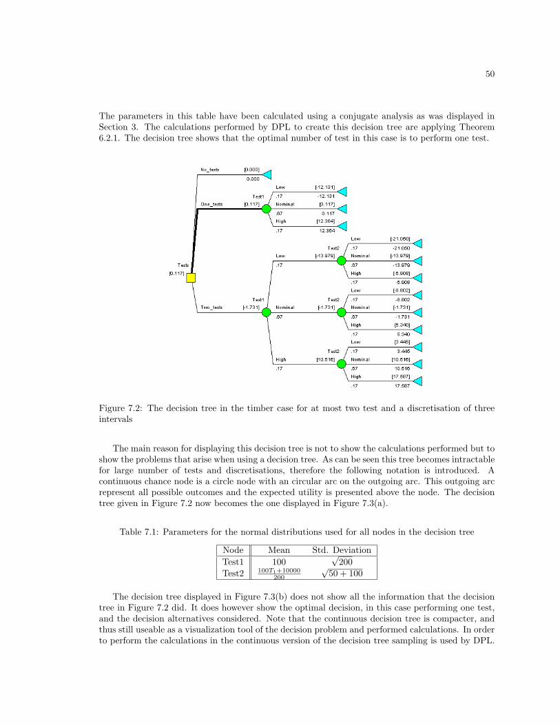
50
The parameters in this table have been calculated using a conjugate analysis as was displayed inSection 3. The calculations performed by DPL to create this decision tree are applying Theorem6.2.1. The decision tree shows that the optimal number of test in this case is to perform one test.
Figure 7.2: The decision tree in the timber case for at most two test and a discretisation of threeintervals
The main reason for displaying this decision tree is not to show the calculations performed but toshow the problems that arise when using a decision tree. As can be seen this tree becomes intractablefor large number of tests and discretisations, therefore the following notation is introduced. Acontinuous chance node is a circle node with an circular arc on the outgoing arc. This outgoing arcrepresent all possible outcomes and the expected utility is presented above the node. The decisiontree given in Figure 7.2 now becomes the one displayed in Figure 7.3(a).
Table 7.1: Parameters for the normal distributions used for all nodes in the decision tree
Node Mean Std. DeviationTest1 100
√200
Test2 100T1+10000200
√50 + 100
The decision tree displayed in Figure 7.3(b) does not show all the information that the decisiontree in Figure 7.2 did. It does however show the optimal decision, in this case performing one test,and the decision alternatives considered. Note that the continuous decision tree is compacter, andthus still useable as a visualization tool of the decision problem and performed calculations. In orderto perform the calculations in the continuous version of the decision tree sampling is used by DPL.

51
(a) Input continuous decision tree for the simplified timbercase
(b) Optimal decision in continuous decision tree
Figure 7.3: A continuous version of the decision tree in the simplified timber case evaluating at mosttwo tests
In the next subsection an approach is shown how these calculations can be done by the ‘Fixed SizeTest Plan’ approach.
7.4.3 Application Fixed Size Test Plan
This subsection will discuss how the optimal fixed size test plan can be determined for destructivetesting in the (simplified) timber case. The optimal number of tests that is calculated is optimalwith respect to the prior information. Therefore it is called ‘fixed size’ as it does not take intoaccount the information gained from a test result other then was expected with respect to the priorinformation.
As first a quadratic loss function will be used, which will lead to an analytical expression for thecurve displaying expected loss as a function of n. As second a bi-linear loss function is used. Asthird an in practice useable application is given.
Quadratic loss
The following loss function is used9
LF (r, d(n), n) = L(r, d(n)) + C(n), (7.4.4)
where the decision loss function is taken as L(r, d(n)) = K(d(n) − r)2. Note that this (quadratic)decision loss function displays the loss in taking the decision to estimate R by d(n). Note that inthe timber case not the inference problem needs to be solved, the optimal number of tests needs tobe solved. Thus the decision is made on n which implies a value for d. The quadratic loss functionwill be used to calculate the minimal posterior expected loss for a fixed number of tests (n), thusthe decision is made to perform n tests. This is by definition the Bayes Risk. This risk (expectedloss) is minimized over all n and the optimal fixed size test plan is found. Formally this approach
9Note that the super index indicates that it is the total loss for the fixed size test plan, thus including test costs.

52
is defined by Theorem 7.3.2. Applying this theorem in the simplified timber case (see Chapter 2)gives the following.
As quadratic loss is used the Bayes decision rule equals the posterior expectation10. This meansthat the Bayes risk in this case equals
BR(n) = EREDn|R[LF (r,E(R|Dn), n)]= EDnVar(R|Dn) + C(n)
= Kσ2σ2
µ
σ2 + nσ2µ
+ C(n). (7.4.5)
Figure 7.4: The decision loss against the number of test in the timber case
Again the cost of testing are taken proportional to the number of performed tests, i.e., C(n) =nCT . A plot of the curve defined by Equation (7.4.5) is displayed in Figure 7.4. From this figurea clear minimum can be derived. This can also be done exact by taking n to be continuous andsetting the derivative of BR(n) to 0 (∂BR(n)
∂n = 0), which gives
n =σ√K√CT
− σ2
σ2µ
. (7.4.6)
Now the optimal fixed size test plan is that non-negative integer n closest to n.The followed approach gave the optimal fixed size test plan in the simplified timber case due to
the following three reasons. As first, due to the use of a quadratic loss function a Bayes decisionrule is easy found as the posterior expectation. Therefore the Bayes Risk is defined as the posteriorvariance. The second reason is the existence of an analytical predictive distribution. This impliesthat an analytical expression can be found for the posterior distribution. Together with the firstreason gives an analytical expression for the expected loss, in this case the variance of the posteriordistribution. The third reason is that the posterior loss is independent of the test results, only thenumber of tests performed. This implies that the posterior expected loss is still equal to the posteriorvariance. All of these reasons together give that an analytical expression is found for the optimalfixed test size.
It is very nice that an analytical expression is found for the fixed size test plan in the simplifiedtimber case, still this does not represent a very realistic situation for two reasons. First the quadratic
10The proof of this is given in Appendix A.4.

53
loss function is symmetrical, which implies that overestimating the strength of the timber is equallypenalized as underestimating the strength. As can be imagined this is not very realistic from thedesign and producers perspective. For instance from a design perspective clearly overestimating willlead to more (possible) failures and repair costs, which compared to the costs of underestimation willbe greater and thus not symmetrical. Second the simplified timber case is not very realistic, and wasonly used for its analytical predictive distribution. Therefore another loss function is investigated.
Bi-linear loss function
A partial linear (non-symmetric) loss function will be investigated. The bi-linear loss function isdefined below for inferring d(n) by deciding to perform n tests and the true strength(R) equals r.
Definition 7.4.1. The bi-linear loss function is defined as follows
L(d(n), r) =
c1(r − d(n)) r ≥ d
c2(d(n)− r) r ≤ d(7.4.7)
where c1, c2 ≥ 0.
Typically in determination of the strength of a material in the context of reliability c2 > c1. Thiswas already mentioned from a designers perspective as overestimation is heavier penalized thanunderestimating. When using the bi-linear loss function the Bayes decision rule becomes 100 c1
c1+c2-
percentile estimate of the predictive distribution of R, which is proven in Appendix A.4. As theBayes decision rule is the 100 c1
c1+c2-percentile estimate of R an interesting interpretation to c1 and c2
can be given. The reasoning is as follows, as it is common to take the 5-percentile of the predictivedistribution of R as the characteristic strength a condition on the ratio of c1/c2 is put as 1/19. Thisratio is very helpful when defining the decision problem. Defining the cost of overestimating canoften be done, but defining the cost of underestimation are much harder. By the defined ratio onlyone has to be determined and the other is automatically given by the ratio.
Using the bi-linear loss function and the decision rule does not lead to an analytical expression forthe posterior expected loss as a function of the number of performed tests. This can be contributedto the fact that the expectation that need to be calculated cannot be performed analytically. Usinga sampling techniques to calculate this expectation is implemented in a procedure in the nextparagraph. As a new procedure needs to be written for this, it is not applied to the simplifiedtimber case but straight to the (general) timber case.
Numerical solution
This paragraph will show how the ‘fixed size test plan’ can be determined in the timber case usingsampling techniques and the analytical approach or the BBN approach. In order to perform theupdate analytically the NIG-model is used. Also a new loss function is used which has an actualinterpretation.
The following input has been received from the timber producer to define the decision problem.Table 7.2 gives the information needed to define the utility function. It is also given that the pricedifference between timber from two adjoining strength classes is 10 percent. The classification forthe timber under investigation is given in Table 7.3. The prior information for this kind of timberis given as m = 80,Λ = 8, α = 8, β = 0.0005.

54
Table 7.2: Input for decision problem
Desciption ValueBatch size 100m3
Beam size 0.1m× 0.2m× 4mPrior price 500EUR
m3
Cost of manhours 85EURTest time 1 hour
Table 7.3: Classification of characteristic strength (NEN6760)
Class I II III IV V VI VIIStrength 0-30 30-35 35-40 40-50 50-60 60-70 70-200
Using the give information makes it possible to define the decision problem in format that itcan be solved by the fixed size test plan approach. Using the producers approach to formulate thedecision problem leads to the following considerations. The batch of timber(100m3) is graded andthen tests can be used to improve the grading. The timber is graded by calculating the characteristicstrength RChar from the (predictive) distribution as the 5-percentile point. This point is then gradedinto a strength class with Table 7.3. The graded characteristic strength of the batch (RG) is givenas the left bound of the class. Notice that when the actual characteristic strength (RChar) is below30 it is graded as strength class I. Timber in strength class I has a graded characteristic strength ofRG = 0 and is thus useless.
From a producers point of view a clear interpretation can be given to the loss function and thetesting costs. The costs of destructively testing a beam from the batch is given as the price of thebeam and the cost of the man-hours needed to perform the test. This implies the cost for this kindof test given as
C(n) = 125n. (7.4.8)
The decision loss can be given as a function of the determined strength class of the batch. If thestrength class is not changed after testing the loss equals 0. If the expected strength class aftertesting is one class lower the loss is given as the batch size times the difference in sale price of thetimber in the different strength classes. The same holds for the expected gain when the expectedstrength class is one larger the loss is given as the batch size times the difference in sale prices11.Note that the maximal loss is given to when the strength class becomes I, then it equals the batchsize times the price of the prior strength class, this as the batch cannot be sold. Now the decisionloss and the cost of testing have been determined the loss function has been determined which meansthat the expected loss for the fixed size test plan can be determined. This is done using the pseudocode given below. The result will be a plot of the expected loss against the number of performedtest, from which the optimal test size can be determined.
Pseudo Code ‘Fixed Size Test Plan’ Using Sampling
Initialization
• Define constants,11Notice that this difference is now negative thus there is no loss, gain.

55
• Define prior information,
• Define strength classes,
• Define utility function,
• Process prior information,
Computation (loop over number of runs(i))
• Loop over number of samples(j)
– Sample ηi,j , µi,j ,– Loop over number of tests(k)
∗ Sample destructive data, di,j,k
∗ Calculate sampled characteristic strength(perform update) rChari,j,k ,
∗ Classify sampled characteristic strength rGi,j,k,
• Calculate expected loss,
Post processing
• Plot expected loss against number of test for each run.
This pseudo code is implemented in MATLAB as,‘SampleME8.m’(see Appendix C). The resultsof this m-file are displayed in Figure 7.5. From this figure it is determined that four tests shouldbe performed. Multiple curves have been plotted in this figure to display the convergence of thesampling used to determine the expected loss.
The m-file that produced Figure 7.5 uses a special approach to sample destructive tests. Thepseudo code also showed this, the parameters M,H are sampled and then used to generate samplesfor the destructive test results. It is important that it is done in this order as given these sampledparameters M,H the test results are independent. Then on the basis of these sampled test resultand the prior information a sampled characteristic strength is determined. In ‘SampleME8.m’ ananalytical approach is used for this, by application of the NIG-model12. By use of this model thecharacteristic strength can be given in terms of the parameters of the prior distribution and thesampled test result, this is formulated in the following proposition.
Proposition 7.4.1. The characteristic strength of the timber (0.05 percentile point) when using the
NIG-model is given in the parameters of the NIG-model, see Equation13 (5.1.7), as
RChar = m∗ +
√1 + Λ∗
β∗α∗Ψ−1
T (0.05, 2α∗), (7.4.9)
in which Ψ−1T (0.05, 2α), denotes the inverse cumulative distribution function of a standard student’s
t-distributed variable.
Proof. The proof of this proposition is listed in the Appendix A.3, which constitutes of rephrasing
Equation (5.1.1).

56
Figure 7.5: A plot of the expected loss against the number of tests
The use of an analytical approach to perform the update and thus determine the sampled char-acteristic value is not necessary. The updating can also be done otherwise, numerically or by aBBN. For the timber case using the NIG-model also a MATLAB program was created that uses aBBN approach (HUGIN) to perform the update. This programm is added in the Appendix C, as‘SampleMEHugin4.m’. Note that this m-file is implemented using the same pseudo code only thestep calculate sample characteristic strength is done by HUGIN. By comparisons of the results ofboth the codes using HUGIN and the analytical approach it is concluded that they give the sameresults. The main reason for adding this code to the appendix is that it can easily be applied inother situations and other decision problems. Using the BBN approach for the updating also hasanother advantage. The graphical model defined in the BBN approach essentially gives the samplingorder, as only prime nodes are sampled. This is discussed in Chapter 8.
7.4.4 Application VOI
Using the value of information to create an optimal test plan needs a more mathematical formulationof the decision problem. The decision problem to determine the optimal fixed size test plan can thusformulated as
S, the states of the world si denotes the state of the world, e.g. the prior characteristic strength;
F , the set of acts fn perform the n proposed tests;12This model is defined in Chapter 4 and applied in Chapter 5.13To determine the characteristic strength (RChar) prior to testing use the parameters of the prior information.

57
f0 do not perform the proposed test.
C the set of consequences Let the consequences be define over the set of F × S, resulting in:
cn,m the decision has been made to perform n tests and the Bayesian update has been per-formed and using the test results leading to cn,m, e.g. the (updated) predictive characteristicstrength; c0 the decision has been made not to perform the test.
The Utility-function has typically the following form:
U1,...k(c) = U(s, f)−k∑
i=1
κi (7.4.10)
where s is k-dimensional and κi denotes the costs of performing test i.The following considerations derive the optimal test plan. A test is added to the test plan, i.e.
is performed whenν(F |Tp → Tp ∪ T ) 6= ν(F |Tp) (7.4.11)
Where Tp denotes the test plan. Which is equivalent to stating
ν(F |Tp ∪ T ) > ν(F |Tp) (7.4.12)
This gives the following criteria for constructing a test plan:
Test 1 The first test is performed when
ν(F |T1) > ν(F |∅) = ν(F ) (7.4.13)
Using the definition for the value of information in Equation (7.4.13) defines the followingrestriction on the cost of the first test.∑
d1∈D1
p(d1)maxf∈F
∑c∈C
p(f−1(c)|d1)U1(c) > maxf∈F
∑c∈C
p(f−1(c))U(c) (7.4.14)
All the probabilities in Equation (7.4.14) are known/ given by the priors or and iff the testoutcome is known. Thus by solving this equation for the cost of a test gives a condition onthe costs of a test.
Test 2 The second test is performed when
ν(F |T1 = t1, T2) > ν(F |T1 = t1) (7.4.15)
By definition this means∑d2∈D2
p(d2|D1 = d1)maxf∈F
∑c∈C
p(f−1(c)|D1 = d1, D2 = d2)U1,2(c) >
maxf∈F
∑c∈C
p(f−1(c)|D1 = d1)U1(c)
This equation needs to be solved for the outcome of test one giving a condition on the outcomeof test one to either perform the second test or not.
This approach does not seem to give an feasible approach as for each utility and probability a pre-dictive distribution needs to be calculated. This gives to much computations. Also the formulationof the decision problem in this setting does feel a bit unnatural. Possibly it can be formulated asaccepting the sample or rejecting the sample as possible acts. This is then added as future research.

58

Chapter 8
General Method for Testing
8.1 The General Method
This chapter demonstrates the use of the theory derived in the previous chapters. It can be seen asan attempt to create a complete methodology which stipulates the use of testing/observations. Thefollowing general method is proposed
General Method for Testing
Problem definition
1. Define testing objectives and decision problem,
2. Create models,
3. Define primary variables,
Interpretation of test results
4. Apply Bayesian method,
5. Validation of Bayesian method and models,
Test plan
6. Define optimal test plan,
Evaluation
7. Interpret results.
There are two main steps in this method, respectively the fourth and sixth step. All other stepsare preparations for these main steps or checks of these two main steps. The time when the firstsix steps are performed is different from the last step. The first six steps are performed before thetests are performed and in step seven the test results are available and are investigated. This is anessential difference. Note that for performing the seventh step the method defined in step four canbe used. Also note that often this method will be performed in a loop. After the seventh step oftena new decision problem is formed to determine if it is useful to perform additional test given the new
59

60
information gained from the tests. The result can be to perform even more tests, which does notimply that the first application of the method has failed. It only means that the information gainedfrom the tests is more or at least different then was expected. The following section will show anapplication of the method.
8.2 Humidity Case
The case that will be used to demonstrate the proposed method for testing is referred to as thehumidity case. It addresses the issue of determining the time when the humidity on the outside of aconcrete wall is lower then a predefined level. This case has been derived from the following actualsituation, a contractor wants to apply stucco to a wall. In order for the stucco to stay fixed to theconcrete wall, the wall needs to be dry. Often after some time humidity from within the wall reachesthe outside of the wall and effects the stucco. To avoid this stucco is applied after a pre-definednumber of days. This in order to let the humidity from within the wall to dissipate. This sometimescreates unnecessary delay in the construction as the waiting period is far to long. Now testing isproposed to be used to determine when the wall is dry enough, and not use the pre-defined numberof days. This in order to decrease the time that needs to be waited till the stucco can be applied.
In order to model the movement of the humidity a small simplification in the modelling of thehumidity movement within the wall is used as it is modelled as one-dimensional. In Figure 8.1 awall under investigation is displayed schematized displaying the mentioned simplification.
Figure 8.1: Schematized view of a wall under investigation
In this figure a distance (dWall) is displayed, this is the average distance the humidity needs to

61
Table 8.1: Input for decision problem
Desciption ValueWall thickness 35mmFixed cost of performing tests 100EURCost of performing a single measurement 15EURSensor size 3 measurement pointsSavings 500EUR/week
travel to reach the stucco1. Also a sensor is displayed in Figure 8.1. This special sensor measuresthe humidity at different depths, referred to as measurement points (a(n) (observation) model forthis sensor will be defined later). The use of this sensor defines the decision problem, which canbe phrased as, how many measurements with this kind of sensors should be performed to optimaldetermine the time till the stucco can be applied. Now that the case is briefly introduced the generalmethod for testing can be applied.
Define testing objectives and decision problem
In this case the objective is to investigate if it is possible to determine, with testing, the time whenthe humidity in the wall has dropped to an acceptable level. This analysis will take into accountthe expected benefits and costs of testing. The decision problem can be defined as: how many testsare ’ideally’ needed to determine the time when stucco can be applied. Notice that the time whena test is performed is taken as fixed. Table 8.1 gives the parameters that specify the constructionunder investigation and the decision problem.
Create models
To model the movement of the humidity in the concrete wall the following relation is used to describethe distance the humidity travels in time.
D(t) = Rv
√t. (8.2.1)
In which time is denoted as t in [days] and the humidity intrusion rate as Rv in [mm/days12 ]. Note
that Rv is assumed to be time independent. From experience gained from previous experimentsRv is assumed a-priori to follow a log-normal distribution2 with mean 2[mm/day
12 ] and a standard
deviation of 1[mm/day12 ]. This relation is used to describe the distribution over the time needed
for the wall to be dry at the outside of the wall. The humidity that is present in the concrete wallis modelled to travel (on average) a distance dWall. Together with Equation (8.2.1) this gives thefollowing model for time needed by the wall to be dry on the outside of the wall,
TDry =(dWall
Rv
)2
. (8.2.2)
This in terms of the Bayesian method is the ‘forward model’, see Chapter 3.1In case of of solid concrete wall this distance can be thought of as half the wall thickness.2The parameters of this distribution are M = 0.5816 and V = 0.4724.

62
As mentioned earlier the observations/measurements are done with a sensor, this sensor measuresthe specific resistance in the concrete at three different depths (positions) in the wall. The depthswhere the measurements are taken are placed at a fixed distance from each other. Thus a singleobservation is represented as a vector containing specific resistance measured at each depth. If thissensor has q measurement points this is denoted as
Ωm =[Ω1
mΩ2m · · · Ωq
m
]′. (8.2.3)
The following three (observation) models describe the relation3 between the measurements andthe humidity intrusion rate (Rv).
Measurement accuracyΩi
m = Ωirεi. (8.2.4)
Conversion error
Ωir =
1B
log(V i
A
). (8.2.5)
Humidity relation
V i = v0 −(v0 − vc)Rv
√(t)
xi. (8.2.6)
The first two models describe the error in the measurements, the last the relation between humidityat a location(x) and Rv. The measurement accuracy describes the relation from the measured specificresistance to the actual specific resistance at that depth in the construction, i.e., the imperfection inthe measurement. Where respectively εi ∼ N (1, 0.05) denotes the (multiplicative) error, Ωi
r the realspecific resistance [Ωm] at depth i, and Ωi
m the measured specific resistances [Ωm] at depth i. Theconversion error models the error induced by the (empirical) relation between specific resistance andhumidity. As a result this error is the same for all measurement points. A and B both have a-priorinormal distributions4 with respectively mean 150.18[kg/m3], 1.21∗10−5[Ω−1m−1] and variance 0.05and 0.1. Respectively the humidity relation described by Equation (8.2.6). This equation describesthe relation5 between the humidity(V ) present in the wall and the humidity intrusion rate (Rv).
When multiple measurements are performed they are thus performed in ensembles of three mea-surements. The models given above do not (yet) take into account (spacial) correlation. Thereforemultiple measurement can only be used to learn about the conversion error and thus better deter-mine the humidity intrusion rate (Rv). This can be defended by assuming homogenous humidityover the surface of the wall. Also a model for the cost of testing is needed to solve the decisionproblem, which in this case is a linear cost function,
C(n) = CS + nCT . (8.2.7)
In which CS denotes the (fixed) setup cost for testing describing the costs made to develop or buythe sensor, CT the cost of performing a test and analyzing the data received from a sensor. Thedecision that needs to be made is to define a number of tests to perform at a specific point of time.
3Note that this defines the likelihood function.4As a first approximation the errors are modelled as independent.5Using this relation to describe the relation between the humidity present in the wall and the rate of intrusion
is not completely correct for a wall under inspection. This model was derived and implemented in this case duringthe process of defining the Bayesian method and was then fully applicable. However the case specifics changed whendefine the decision problem and this model was still used as no time was left to create another more appropriatemodel. This does not have important consequences for the demonstration of the method. Only the results of the caseare not completely true as the update is not done correct.

63
Table 8.2: Conditional probability table of node error1 in HUGINExpression Normal(1,0.05^ 2)-inf - 0.95 0.1586550.95 - 1 0.3413451 - 1.05 0.341345
1.05 - 1.1 0.1359051.1 - inf 0.02275
Define Primary Variables
Now all models have been defined, the stochastic variable to which the Bayesian method will beapplied needs to be defined. From all the models, Rv is identified as the random variable to whichthe Bayesian method will be applied. Still the random variable of interest is TDry. Actually duringthe derivation of the models these variables were already identified as the primary variables. Howelse would all the models be created? This step is placed in the method to emphasize that this needbe done. In practice this step is integrated into the previous step.
Apply Bayesian Method
We will start the Bayesian Method by using the graphical representation of the method and substi-tuting into it the actual models and stochasts. This will structure the process. As first the relationsbetween the stochastic variables are defined. We start of with the general graphical formulationgiven in Figure 3.1, now we define the proper stochastic variables which results in Figure 8.2(a)(displayed on page 66). Then we define the predictive model in the graphical representation. Themodels that are inserted are shown in blue boxes. Next the observation models are inserted for onemeasurement point, again blue boxes are used. Finally an entire sensor is modelled in Figure 8.2(d).
This graphical representation is used to model the Bayesian method with a BBN. This is of coarsenot a coincidence, the BBN-approach is chosen as it can easily be constructed from this graphicalmodel. The graphical part of the BBN is almost the same as the graphical model displayed byFigure 8.2(d). The main difference is that names of the nodes are displayed and not the completemodels. These models are used in the quantitative part of the BBN, defining the arcs in the BBN.The result of this graphical part of the BBN in HUGIN is displayed in Figure 8.3 (on page 67).
Defining the graphical part of this BBN is only the start of the modelling using a BBN, nowthe quantitative modelling needs to take place. As set out by the Bayesian method first the priorinformation needs to be entered. This means that the prior distribution for all primary nodes,i.e. Rv, A, B, Error1, Error2, Error3 needs to be defined. Notice that this is actually imple-menting the information given in step one of the method. For example it was formulated thatthe measurement accuracy can be described with Equation (8.2.4) in which the error-term nodes(Error1, Error2, Error3) follow a normal prior distribution. This is then implemented in the quan-titative modelling part of the BBN. As HUGIN performs discrete calculation a discretisation needsto be defined for this node (and for all other nodes in the BBN). As the prior distribution has mean1 and std.dev. 0.05 the discretisation displayed in Table 8.2 is used. Now the prior distribution canbe entered6, in this case a model is used7 in HUGIN, resulting in the following CPT, see Table 8.2.
As can be seen in Table 8.2 two states have been added to create a full support for the distributionof the error-term. This is only to ensure a correct definition of the problem in HUGIN.
6This is also done with MATLAB see the Appendix C all m-files containing Hum.7This is not necessary, tables can also be filled manually.

64
The second step in the Bayesian method is to define the likelihood. This is done in HUGINby defining models for the CPT of the nodes that appear in the observation models. When this isdone the entire BBN is defined and can be used to perform the update and perform inference, whichconcludes the Bayesian method. The entire network was created in MATLAB and the code can befound in the Appendix C as ‘HumCreateNW.m’.
Validation of Bayesian Method and Models
This next step in the method is to ensure that the previous steps have been performed correctly. Byentering possible observations and subsequently performing the update the output of the Bayesianmethod is checked for errors. Often small adjustments in previous steps in the method need be made,e.g. discretisations need to be adjusted. Also it serves as a check to see whether the important factorshave been identified and it shows what kind of testing should be done.
In this application of the general method we have proposed to use HUGIN (and MATLAB) toperform the Bayesian method, as this is a robust approach and easy to implement as it is constructedin a very natural way. It can sometimes be more efficient to use other methods discussed in chapter4. In the humidity case also the direct numerical integration approach has been used. This to checkwhether HUGIN was used correctly to perform the update and to see the difference between the twoapplications. This is omitted in the appendix in subsection A.5.
Define Optimal Test Plan
In this step of the method the test plan has to be derived. This means solving the decision problemdefined in the first step. In order to do this three possible approaches were given in Chapter 7.During the thesis research a combination of the ‘Decision tree’ for visualization purposes and ‘Fixedsize test plan’ approach for calculations was found to be very useful, the latter of these is thus used.The following parameters were gathered for the decision problem in the first step. These parametersare used to define the utility(loss) function. This function will be used to measure the effects(gain)of performing tests and the costs. The costs are modelled as being independent of the test resultand only dependent on the number of performed tests. The fixed cost of performing test are givenas 100EUR. The (variable) cost of performing a single test are given as 3 ∗ 15EUR = 45EUR atest. These variable costs are the cost of performing a measurement, e.g. cost of transmitting testresults from sensor to computer or power needed to use the sensor, and costs for interpreting thetest results. These numbers can be substituted into Equation (8.2.7) leading to the cost function.
In order to measure the effect(gain) of performing a test the following considerations are used.Note that the following reasoning can be seen as using the ‘producers approach’, see sub-sections 7.2and 7.4. The forward model is used to determine the time till the wall is dry, see Equation (8.2.2).Using this model gives a distribution over the time till the wall is dry. The regulations do not givea distribution over the time till the wall is dry but give a number of days to wait till the wall isdry(T rule
Dry ). Using this pre-defined number of days that are needed to wait, which in this case is 90days after construction of the wall is complete, gives a bounded region for TDry. The contractorthat needs to apply the stucco does his scheduling of his work at the beginning of the week. Thisimplies that he is indifferent if TDry changes within the range of a week as he cannot change hisschedule to act upon this information. This then defines the discretisation for the domain of TDry
as 0 to 84 with steps of 7 days. Which means in HUGIN the following discretisation given in Table8.3. If the time the contractor has to wait shortens with a week he makes 500EUR.
As mentioned, the result of using a test is reflected in the distribution of TDry via the predictive
65
Table 8.3: Discretisation for TDry in HUGIN-inf-0 0-7 . . . 77-84 84-inf
(forward) model. The regulations do not specify a distribution but give a fixed number, T ruleDry . In
order to compare the effects of the test result the predictive distribution over TDry is used to give anew point estimate of the time till the wall is dry. This is referred to as using a decision rule. Thisdecision rule is thus needed to measure the effects of testing, i.e. to formulate a loss function. Inthis case the 80-percentile point8 of the predictive distribution for TDry is used as T pred
Dry (n). Thisestimate gives the days one has to wait before applying the stucco according to the prior informationand the n test results. Using this information gives the following loss(utility) function.
L(n) = 100 + n35− 500(T rule
Dry − T predDry (n)
)1T pred
Dry (n)<T ruleDry
(8.2.8)
In which 1A<B is the indicator function which means that it is 1 if A < B and 0 if A > B. Equation(8.2.8) clearly shows that reducing the waiting time with a week results in 500EUR at the cost ofperforming the needed tests, and also that if the tests lead to an estimate that is equal or larger thenwhat the regulations prescribe no gain or loss is achieved as the contractor will use the pre-described9
T ruleDry .
Figure 8.4 has been created using the program ‘HumFinal.m’ which is added in the appendix.This figure is used to determine the optimal number of tests. Figure 8.4 clearly shows a minimumwhen performing nine tests. Again multiple curves have been plotted to show that the sample sizeused is sufficient large.
Interpret Results
As the test plan has now been derived the tests can be performed. For interpreting the test results(observations) the Bayesian method can be re-used, which was already implemented prior to testingthus the procedures defined then can be re-used for this. Depending on the results the method isfinished or initiated again taking into account the information gained from the testing.
If an adaptive test plan has been created there will be a loop from this step to previous stepsuntil the testing is completely done as defined by the adaptive test plan (stopping criteria reached).Thus completing the method.
8In this case the 80-percentile point was chosen to create a decision rule. Another approach can be to use the priorinformation on Rv and calculate the prior predictive (cumulative) distribution function of TDry . Then check whichpoint corresponds with the one given by the regulations and use that as the decision rule. This is however subjectto the prior information used. In cases in which no clear decision rule can be found and strong prior information isavailable it can give a solution.
9Which makes him non liable if the stucco fails as he has used the rules, thus no extra loss. Although the contractordid know that the stucco would probably be effected by the humidity indicated by the (ignored) test results.

66
(a) Stochasts defined (b) Forward/predictive model defined
(c) Observation model defined (d) Multiple Measurements
Figure 8.2: Building the graphical representation of the Bayesian method

67
Figure 8.3: The graphical model for the humidity case

68
Figure 8.4: Results of the fixed size test plan approach in the humidity case

Chapter 9
Conclusions, Recommendationsand Further Research
9.1 Conclusions
In this thesis a general method was defined that tells how to test. The method was shown to solvethe problem of defining the number of tests that need to be performed. This was done by takinginto account the expected information received from a test result and the cost of performing a test.
The general method for testing consists of two main elements namely the interpretation of testresults and the decision what test results to obtain. The Bayesian method was applied for theinterpretation of the test results and Savage’s decision Theory was used for the decision part. Fourdifferent approaches to apply the Bayesian method were discussed in this thesis. It can be concludedthat the Bayesian belief network (BBN) approach is the best approach to use in a general setting.This as the BBN approach contains a graphical model which simplifies communication of the usedmodels. Another advantage of using the BBN approach is that it requires minimal mathematicalknowledge of the user, multiple software packages( i.e. HUGIN) can be used for that. These softwarepackages can also be helpful developing a numerical tool for the general method as they can be used.Also in the BBN-approach after the problem is defined it can easy and fast process different (new)data within the model.
The decision part in the general method consists of two aspects, namely definition and calculation.For the calculation of the solution to the decision problem, which means deriving an optimal numberof tests to perform, three approaches have been proposed, namely the decision tree, fixed size testplan and value of information approach. It can be concluded that the fixed size test plan easilycalculates the solution and that the decision tree can best be used for visualizing the performedcalculations.
Two cases, the timber and the humidity case have been discussed and solved with this generalmethod. The result of this is a series of m-files that implement the method. These m-files were setup in a general formulation that they can easily be reused or adapted to other cases. Making thecombination of all these m-files a blue print for a (numerical) tool to solve these decision problems.These m-files running in MATLAB also use the HUGIN-engine to perform the calculations. Thiswas done by controlling HUGIN via MATLAB trough the HUGIN API, a report was added to theappendix explaining how this is done.
69

70
9.2 Recommendations
The following recommendations are made on the use of the Bayesian method. It was concluded thatthe best approach to perform the Bayesian method was the BBN approach. This is only true as itis easy understood and very robust. In some cases using one of the other four given approaches (seeChapter 4) can very well lead to faster and more detailed results.
Another recommendation is that when defining models also bear in mind that the IG-modelcan be used and not only the N -model. As was shown when discussing the analytical approach a(computational fast) conjugate analysis is sometimes possible when using the NIG-model where itwas not possible with the N -model.
9.3 Further Research
This section sets forth the research that should be done to improve or further develop the generalmethod of testing. The following research topics are given for the general method. The methodshould be applied to more cases to see whether more steps need to be added to the method. Themethod can also be expanded to handle multiple decision objectives. In this thesis only the numberof tests were investigated as a decision objective but other objectives might be included in themethod, like what location should be used for testing. This will need further refinement of themodels as spatial correlation between test etc. Also further work can be done to create a numericaltool implementing the general method. This can be done by further developing the m-files that havebeen added to this report into a full numerical tool.
Also some further research can be done on the the Bayesian method. The BBN approach canbe further refined in many ways. For instance the BBN approach can be refined to also includecontinuous BBN’s. This will in some cases make the modelling much more natural. Also theBBN approach as discussed (using discrete BBNs) can be further automated, by automating thediscretisation definition. In this thesis all nodes have been discretised by visual inspection of theresults over the discretisation, ideally this will be done by a program and the user need not to worryabout this.
The Bayes linear approach, that did not seem to work in a general setting, should be furtherinvestigated. This in order to fully understand the reasons it did not perform well in a general setting.If this can be found the approach can be improved to make it suitable for a general application orby given bounds on the estimates it gives.
Further research needs to be done on defining the decision problem in a general case. This asfinding a utility function in case of a real problem has shown to be very difficult, even though twoapproaches for this have been given, respectively designers and producers approach. As well definingthe decision problem as a sequential decision problem needs to be investigated. This can possiblygive a more accurate solution to the decision problem posed or speed up calculations.
The approaches that were used to calculate the solution to the decision problems can also berefined and evolved. In thesis only one-dimensional decision problems were solved, like how manytest should be performed. The given approaches can easily be used in higher dimensional decisionproblems, like which combination of test type A en B should be used. In order to do this the modelsshould be upgraded to handle the dependency between different test types and the now visuallychoosing the optimum needs to be replace by calculations1.
The value of information approach needs to be further researched. During the thesis researchthis approach did not seem to work and in the authors opinion it was due to the problem definition.
1Visually determining the optimum is not possible for decision problems involving higher dimensions then two.

Appendix A
Appendices to the Text
A.1 Proof Multiple Destructive Observations
Proof Proposition 5.1.2. In order to prove that the predictive distribution of R is student-t dis-tributed, when n destructive measurements are used, proposition 5.1.1 is used. Therefore it issufficient to proof that the posterior distribution over M,H is NIG(α∗, β∗,m,Λ) when using n de-structive measurements. This proof goes along the lines of proof 4.1.1 on page 16. The likelihoodfunction of n-destructive measurements in the timber case is give as
L(δ) = fD|M,H(δ1 . . . δn;µ, η)
=n∏
i=1
fDi|M,H(δi, µ, η)
= (2πη)−n2 e
− 12η
n∑i=1
(δi−µ)2
. (A.1.1)
Substituting Equation (A.1.1) and the joint-distribution function in Bayes Rule (1.2.2) leads to.
fM,H|D(µ, η; δ) = Cn(2πη)−n2 e
− 12η
n∑i=1
(δi−µ)2 η−α∗− 32 β∗−α∗
√2πΓ(α∗)Λ∗
12e
[− 1
2(µ−m∗)2
ηΛ∗ − 1ηβ∗
]
= Cnη−α− 3
2−n2 e
− 12ηΛ
[(µ−m)2+Λ
n∑i=1
(δi−µ)2]− 1
ηβ
where Cn, Cn are appropriate normalizing constants. Define α∗ = α + n2 , substitution of α∗ and
re-arranging terms results in1
fM,H|D(µ, η; δ) = Cnη−α∗− 3
2 e− 1+nΛ
2ηΛ
[(µ−m+Λ
∑δi
1+nΛ
)2− (m+Λ
∑δi)
2
(1+nΛ)2+
m2+Λ∑
δ2i
1+nΛ
]− 1
ηβ. (A.1.2)
1Notice that the index of the summations have been dropped. This has been done for typographical reasons itshould show i = 1 up to n.
71

72
Also define the following variables Λ∗ = Λ1+nΛ , m∗ = m+Λ
∑δi
1+nΛ , and
β∗ =2β(1 + nΛ)
−β(Λ(∑δi)2 + 2
∑δim− nm2 − (1 + Λn)
∑δ2i ) + 2(1 + nΛ)
.
which results in
fM,H|D(µ, η; δ) =η−α∗− 3
2 β∗−α∗
√2πΓ(α∗)Λ∗
12e−
12
(µ−m∗)2
ηΛ∗ − 1ηβ∗ . (A.1.3)
Equation (A.1.3) clearly shows that the posterior distribution forM,H isNIG(α∗, β∗,m∗,Λ∗) whichconcludes the proof.
A.2 Calculations and Proofs to Propositions Concerning Com-
parison Bayes Linear
Proof Proposition 5.4.1. The definition of the expectation gives us the following integral.
E(R) =∫rfR(r)dr (A.2.1)
Application of LTP results in.
=∫∫∫
rfR|M,H(r;µ, η)fM,H(µ, η)d(r, µ, η)
=∫∫∫
r1√2πη
e−12η (r−µ)2 η
−α− 32 β−α
√2πΓ(α)Λ
12e−
12
(µ−m)2
ηΛ − 1ηβ d(r, µ, η)
=∫∫
µη−α− 3
2 β−α
√2πΓ(α)Λ
12e−
12
(µ−m)2
ηΛ − 1ηβ d(µ, η)
=∫mη−α−1β−α
Γ(α)e−
1ηβ dη

73
Now the following change of variables is performed to transform this integral to a gamma function;1
ηβ = ξ.
E(R) =m
Γ(α)
∫ξα−1e−
1ξ dξ = m (A.2.2)
Proof Proposition 5.4.2. Substitute D, δ for R,r respectively in the proof of proposition (5.4.1).
Proof Proposition 5.4.3. By definition the following expression is available for the variance: Var(R) =E(R2)− (E(R))2. The right hand side of this expression has two parts which will be calculated se-quentially below.
E(R2) =∫r2fR(r)dr
=∫∫∫
r2fR|M,H(r;µ, η)fM,H(µ, η)d(µ, η, r)
=∫∫∫
r21√2πη
e−12η (r−µ)2dr
η−α− 32 β−α
√2πΓ(α)Λ
12e−
12
(µ−m)2
ηΛ − 1ηβ d(µ, η)
=∫∫
(η + µ2)η−α− 3
2 β−α
√2πΓ(α)Λ
12e−
12
(µ−m)2
ηΛ − 1ηβ d(µ, η)
=∫∫
η−α− 12 β−α
√2πΓ(α)Λ
12e−
12
(µ−m)2
ηΛ − 1ηβ d(µ, η) +
∫∫µ2 η
−α− 32 β−α
√2πΓ(α)Λ
12e−
12
(µ−m)2
ηΛ − 1ηβ d(µ, η)
=∫η−αβ−α
Γ(α)e−
1ηβ dη +
∫(ηΛ +m2)
η−α−1β−α
Γ(α)e−
1ηβ dη
= (1 + Λ)β−α
Γ(α)
∫η−αe−
1ηβ dη +
m2β−α
Γ(α)
∫η−α−1e−
1ηβ dη
Again the following transformation is used 1ηβ = ξ.
E(R2) =1 + ΛβΓ(α)
∫ξα−2e−ξdξ +
m2
Γ(α)
∫ξα−1e−ξdξ
=1 + Λ
β(α− 1)+m2 (A.2.3)
The second term on the right hand side is given by proposition (5.4.1). Substituting these two resultsconcludes the proof.
Proof Proposition 5.4.4. Substitute D, δ for R,r respectively in the proof of proposition (5.4.3).
Proof Proposition 5.4.5. In order to derive Cov(R,D) the following integral needs to be calculated.
E(RD) =∫∫
rδfR,D(r, δ)d(r, δ) (A.2.4)
This can be done via application op LTP and using the priors, e.g.

74
E(RD) =∫∫
rδ
∫∫fR,D|M,H(r, δ;µ, η)fM,H(µ, η)d(µ, η)d(r, δ)
=∫∫
rδ
∫∫fR|M,H(r;µ, η)fD|M,H(δ;µ, η)fM,H(µ, η)d(µ, η)d(r, δ)
=∫∫∫∫
rδ1
2πηe−
12η ((r−µ)2+(δ−µ)2) η
−α− 32 β−α
√2πΓ(α)Λ
12e−
12
(µ−m)2
ηΛ − 1ηβ d(µ, η, r, δ)
The order of integration will now be changed. First integration over r than over δ will be performed.
E(RD) =∫∫∫
δη−α− 5
2 β−α
(2π)32 Γ(α)Λ
12
e−12η (δ−µ)2e−
12
(µ−m)2
ηΛ − 1ηβ
∫re−
12η (r−µ)2drd(µ, η, δ)
=∫∫∫
δµη−α−2β−α
2πΓ(α)Λ12e−
12η (δ−µ)2e−
12
(µ−m)2
ηΛ − 1ηβ d(µ, η, δ)
=∫∫
µη−α−2β−α
2πΓ(α)Λ12e−
12
(µ−m)2
ηΛ − 1ηβ
∫δe−
12η (δ−µ)2dδd(µ, η)
=∫∫
µ2 η−α− 3
2β−α
√2πΓ(α)Λ
12e−
12
(µ−m)2
ηΛ − 1ηβ d(µ, η)
Now first perform the integration over µ.
E(RD) =∫
η−α− 32 β−α
√2πΓ(α)Λ
12e−
1ηβ
∫µ2e−
12ηΛ (µ−m)2dµdη
=∫η−α−1β−α
Γ(α)e−
1ηβ (m2 + ηΛ)dη
Here a gamma-function can be recognized. Define ξ = 1ηβ , this results in
E(RD) =m2
Γ(α)
∫ξα−1e−ξdξ +
ΛβΓ(α)
∫ξα−2e−ξ
= m2 +Λ
β(α− 1)
Together with proposition (5.4.1),(5.4.2) this results in Cov(R,D) = Λβ(α−1) .
A.3 Proof Characteristic Value of the Timber
Proof Proposition 7.4.1. From Proposition 5.1.2 it follows that the predictive distribution of R is(generalized) student-t distributed. The (inverse) cumulative distribution function of is found by

75
transforming the probability density function into the standard form. Equation (5.1.1) shows thefollowing pdf.
fR|D(r; δ) =β∗−α∗Γ(α∗ + 1
2 )√2π(1 + Λ∗)Γ(α∗)
(−C2)−α∗− 12 , (A.3.1)
with
C2 = − 1β∗
− (r −m∗)2
2(1 + Λ∗), (A.3.2)
in which the parameters α∗, β∗,m∗,Λ∗ are that of the posterior distribution over2 M,H(µ, η). Noticethat C2 can be restated as
C2 = − 1β∗
(1 +
β∗ (r −m∗)2
2(1 + Λ∗)
)
= − 1β∗
(1 +
α∗β∗
(1 + Λ∗)(r −m∗)2
2α
)
= − 1β∗C3. (A.3.3)
Define C4 = α∗β∗
(1+Λ∗) , substitution of C3 and C4 in Equation (A.3.1) results in
fR|D(r; δ) =β∗−α∗β∗α∗+ 1
2 Γ(α∗ + 12 )√
2π(1 + Λ∗)Γ(α∗)(C3)−α∗− 1
2
=√C4Γ(α∗ + 1
2 )√
2α∗πΓ(α∗)
(1 + C4
(r −m∗)2
2α∗
)−α∗− 12
(A.3.4)
From which a standard student-t distribution can be recognized, with ν = 2α∗ degrees of freedom,adjusted by C4 and shifted over m∗,i.e.,
fR|D(r; δ) =√C4ψT (C4 (r −m∗) , 2α∗) , (A.3.5)
where ψT is the pdf. of a standard student-t distributed variable.
A.4 Proofs Bayes Decision Rules
Theorem A.4.1 (Bayes Decision Rule under Quadratic Loss). Let L(r, d) = K (d− r)2 bethe (quadratic) loss function. Then E(R|X) minimizes the posterior expected loss, eg.
arg mind
∫r
K (d− r)2 fR|X(r;x)dr = E(R|X). (A.4.1)
By definition this implies that the Bayes Decision Rule under quadratic loss is E(R|X) = r.
2These parameters can be expressed in the parameters of the prior information and the test results by Equation(5.1.7).

76
Proof. To find the minima mentioned in Equation (A.4.1) the posterior expected loss is differentiatedwith respect to d and then set equal to 0. The posterior expected loss can be expressed as∫
r
K (d− r)2 fR|X(r;x)dr =∫
r
K(d2 − 2dr + r2
)fR|X(r;x)dr. (A.4.2)
Differentiating and setting equal to zero results in
∂
∂d
∫r
K(d2 − 2dr + r2
)fR|X(r;x)dr =
∫r
K (2d− 2r) fR|X(r, x)dr
= 2dK∫
r
fR|X(r;x)dr − 2K∫
r
rfR|X(r;x)dr
= 2K(d− E(R|X)) = 0 (A.4.3)
Which gives r = E(R|X).
Theorem A.4.2 (Bayes Decision Rule under Bi-Linear Loss). Let L(r, d) be the bi-linearloss function. The Bayes Decision Rule is then the 100 c1
c1+c2-percentile estimate of the posterior
distribution of R.
Proof. To prove the theorem given above the posterior expected loss is calculated and then theminimum is found by setting the derivative of this expression to 0.
ER|X(L(d, r)) =∫ ∞
−∞L(d, r)fR|X(r;x)dr
=∫ d
−∞c2(d− r)fR|X(r;x)dr +
∫ ∞
d
c1(r − d)fR|X(r;x)dr
= c2dF (r)− c2
∫ d
−∞rfR|X(r;x)dr + c1
∫ ∞
d
rfR|X(r;x)dr − c1d[1− FR|X(r, x)
](A.4.4)
The derivative of this expression to d is equal to
∂
∂dER|X(L(d, r)) = (c1 + c2)FR|X(r;x)− c1 (A.4.5)
Notice limd→∞
∂∂dER|X(L(d, r)) = c2 ≥ 0. Thus this expectation is minimized if
FR|X(d) =c1
c1 + c2. (A.4.6)
Therefore the Bayes decision rule for bi-linear loss is given as
r = F−1R|X(
c1c1 + c2
) , r c1c1+c2
(A.4.7)

77
A.5 Direct Numerical Integration in Humidity Case
In this section a derivation of the direct numerical integration approach of the Bayesian methodapplied to the humidity case is given. The first step defining the prior information is exactly thesame as given in subsection 8.2. The next step defining the likelihood is different then was donein section 8.2, as there the HUGIN-approach was used. Here a more mathematical procedure isfollowed. Still the graphical model that was used can be helpful in the derivation as it shows whichtransformations will be performed deriving the likelihood.
The likelihood function is deducted from the observation models given as Equations (8.2.4),(8.2.5), and (8.2.6). By definition the likelihood function is given by the following probabilitydensity function
fΩM |Rv(ωm; r) (A.5.1)
As given by observation model 8.2.5 all measurements at one specific time are dependent on theconversion error. Applying the LTP by conditioning on the error of conversions leads to
fΩM |Rv(ωm; r) =
∫∫fΩM |Rv,A,B(ωm; r, a, b)fA,B(a, b)d(a, b). (A.5.2)
The joint density function is given by the prior information thus concentrate on fΩM |Rv,A,B(ωm; r, a, b).Using the humidity relation ,Equation (8.2.6), on the conditioned variables in this function resultsin
fΩM |Rv,A,B(ωm; r, a, b) = fΩM |ΩR(ωm;−1
blog(v0a− v0 − vc
ar√tinspv0
x
)). (A.5.3)
Now a transformation from Ωm to ε is performed to determine the probability density function.This means using observation model, Equation (8.2.4). The Jacobian for this transformation equals
J = | ∂ε∂ΩM
| = | 1ΩR
|. (A.5.4)
Taking all errors being independent of each other, the transformation results in the following ex-pression.
fΩM |Rv,A,B(ωm|r, a, b) =n∏
i=1
[fε
(ω
(i)m
ω(i)r (r, a, b)
)1
ω(i)r (r, a, b)
]
=n∏
i=1
fε
− ω(i)m b
log(
v0a − v0−vc
ar√
tinspv0x(i)
)− b
log(
v0a − v0−vc
ar√
tinspv0x(i)
) (A.5.5)
Where index (i) indicates at which measurement-position (depth) the measurement is taken.Notice that ε ∼ N (1, 0.05) which implies that in principle a known expression is found for thelikelihood. In principal because the integration over a,b still needs to be performed. This is thusdone by direct numerical integration, which is implemented in MATLAB. The program is added inAppendix C. The next step in the Bayesian method is to calculate the posterior distribution. Thisis done by using Bayes’formula, e.g.
fRv|ΩM(r;ωm) ∝ fΩM |Rv
fRv(r) (A.5.6)
This was also done numerically in MATLAB. The resulting m-code can be used to perform theBayesian method, to perform the update of the stochast Rv, and check if HUGIN did perform theupdate correct (which it did!). This was done by comparing the predictive distribution from HUGINwith the one from direct numerical integration approach.

78

Appendix B
Controlling HUGIN
This section contains a small report describing the use of the HUGIN API’s in MATLAB.
B.1 Introduction
This report explains how HUGIN can be addressed by MATLAB and Visual Basic (for Excel) byusing the HUGIN Application Programming Interface (API). HUGIN has now developed a VisualBasic ActiveX server which makes it possible to access the HUGIN API’s from many differentapplications. Which was previously only supported from C-libraries.
The emphasis in this report is mainly on use of the API with MATLAB. Briefly usage fromVisual Basic is discussed, this because the available help file on the ActiveX Server is based on VisualBasic. This help file1 can be found in the HUGIN installation directory as The HUGIN API ActiveXServer 6.3 Help. This help file also contains some elementary examples and the API referencemanual. This reference manual is needed for reference to available object properties and for referenceto all possible functions.
This report can be read without any pre-knowledge of the HUGIN ActiveX server, still basicknowledge on belief nets is needed. To understand this report elementary knowledge of the VisualBasic programming language is needed (only for chapter 2) and knowledge on the use of MATLABis needed. This report was based on usage with MATLAB 7 Release 14. If one uses another versionsome commands might not be executed. This is due to changes in different version of MATLAB inthe function ’invoke’.
1When in this report one is referred to ’the help file’, without any reference to a specific help file this help file isintended.
79

80
B.2 Installation
Installation in Windows
During the installation of HUGIN Researcher, the HUGIN API’s are placed in their own subfolderin the main installation folder. Another file is placed in the windows system32 folder, namelynphapi63.dll 2. Before this file can be used by Windows it needs to be registered with Windows.This should be done automatic during the installation but often this does not happen and thereforeperform the following steps to do this manually. Open a dos-box in windows. And execute thefollowing command regsvr32 hapi63.dll from \HDE6.3X\lib-directory which is a subdirectory ofthe HUGIN installation-directory. Now the server can be used in general applications, e.g. MAT-LAB. How this is done will be explained in chapter B.4. The next subsection will explain what todo in order to use the HUGIN API’s in Visual Basic for Excel (VB).
If problems occur trying to access the HUGIN API’s one should look in the HUGIN release notesto solve the problem or e-mail HUGIN at [email protected].
Library in Visual Basic
In order to use the HUGIN API’s in VB the HUGIN ActiveX library needs to be added to thereferences of VB. This is done by selecting from the ’tools’-tab ’References’. Now a windowis displayed with all the references that VB currently uses. Now tag the box with HUGIN APIActiveX Server 6.3. If this library is not in the list, select it via ’Browse...’ from the API instal-lation directory by selecting hapi63.dll. Now one can use the API’s in VB, how this is done willbe explained in chapter B.3.
B.3 Visual Basic for Excel
This chapter describes how to use some functions from the HUGIN API and how to change propertieswith the HUGIN API. Only the most basic functions are treated here by giving examples. It is meantto illustrate the syntaxis for using the API in VB. This section can be seen as an addition to theexamples in the help file.
Small Example 1
As first the small network displayed by figure B.1 will be created with the help of VB.
Figure B.1: The Example network in HUGIN created via VB
2For some reason this is not always the case thus if this file is not found there after installing HUGIN; place thisfile manually there. This can be done by copying the file from the HUGIN directory

81
The code needed to create this network is displayed below. In the next subsections each of thecommands issued will be explained.
Public Sub Example()’ Load the ActiveX ObjectSet glob = CreateObject("HAPI.Globals")’Create a BBNSet Domain = glob.GetNewDomain()’Create NodesSet ndA = Domain.GetNewNode(hCategoryChance, hKindDiscrete)ndA.Label = "A"ndA.Name = "A"Set ndB = Domain.GetNewNode(hCategoryChance, hKindDiscrete)ndB.Label = "B"ndB.Name = "B"’ Add StructureCall ndA.AddParent(ndB)’ Save NetworkCall Domain.SaveAsNet("C:\ExampleE.net")
End Sub
General Commands
In order to do any work with HUGIN in VB one needs to create an object in VB to handle alloperations called or performed from the API. This is done with the following command.
Set glob = CreateObject("HAPI.Globals")
Handling a Network
The following code loads a network from a HUGIN file into the ActiveX object which was createdin VB by the previous code. Then this code saves the network into another HUGIN net-file.
Set domain=glob.LoadDomainFromNet("C:\BBN1.net", Nothing, 0)Call domain.SaveAsNet("C:\BBN2.net")
The arguments ’Nothing’ and ’0’ are additional arguments which are set to these values becausethey are not used here. The possibilities for using these additional arguments are explained in theAPI reference manual contained in the help-file.
Creating Nodes
The following code will create a node and define its type, name, and label. It is important to noticethat name and label are different properties of the node. The name of a node is how HUGIN refersto the node. This implies that it must be unique for each node. According to the API tutorial thename needs to be specified in a format similar to C-identifiers. This means ’loosely’ that no spacesand funny characters may be used in names. The label of a node is the name that is displayed in anode in the graphical interface.

82
Set ndA = Domain.GetNewNode(hCategoryChance, hKindDiscrete)ndA.Label = "A"ndA.Name = "A"
Other properties of a Node can be defined/altered using set in the same way as with label and namewas done. All properties available for a node can be found in the API reference manual.
Adding Structure
Once the nodes are created in the network the structure can be added. Structure is added in thevisual Interface of HUGIN by drawing arcs from one node to the other. This is done from theHUGIN API with the function ’AddParent’.
Call ndA.AddParent(ndB)
Notice that the function ’AddParent’ is called from the child node.
Editing States
When a discrete node is created in the network one still needs to define the discretisation. Thissection shows how to define/change the number of states and how to change the State Values.
ndA.NumberOfStates = 2ndA.StateLabel(0) = "On"ndA.StateLabel(1) = "Off"
The code displayed above changes node A to have two states; ’On’, and ’Off’. The index used inthe property ’StateLabel’ starts at 0. Therefore the state ’On’ was set with index 0. HUGIN startsevery index with a 0. Notice when setting the boundaries of a node of type ’Interval’ the index todefine the values of the boundaries of the intervals start also at 0. The following figure shows threeintervals [7, 10], [10, 13], [13, 16] at each boundary the value of the index needed in HUGIN to accessthis boundary is displayed above it.
Figure B.2: A plot of an interval with the index used in HUGIN
Filling Tables
The next code will display how to manually fill a (conditional) probability Table of a node.
ndA.Table.Data(0) = 666

83
Notice that the property ’Data’ has an index attached to it. This index displays the entry in thetable. The following definition gives the value of this index for each table entry.
Definition B.3.1. Let TA be the table of node A which has m columns and n rows (TA is the(conditional) probability table of node A). The index needed in the property data for element TA(i,j)is defined as
Index(i, j) = i− 1 + (j − 1) ∗ (n− 1), 1 ≤ i ≤ n, 1 ≤ j ≤ m. (B.3.1)
Bear in mind that HUGIN normalizes all the entries in the table such that the sum of eachcolumn equals 1, when it uses them for computation.
B.4 MATLAB
General Commands
To control HUGIN from MATLAB one has to instantiate the ActiveX server and then use theavailable functions in this library to alter objects created from this library. One can instantiate theHUGIN ActiveX Server into an object in MATLAB with the following command:
glob=actxserver(’HAPI.Globals’);
This command creates a HUGIN API object named glob, which now can be used to address functionsand properties defined in the API. To see what functions are available for this object issue thecommand methodsview or methods, or see the reference manual. Notice that MATLAB makes adistinction between properties of an object and functions defined in the API. This distinction isapparent in the way both are called/issued.
To issue a function (or sub procedure) from the API the command invoke needs to be used. Thiscommand tells MATLAB which object contains the function and which function it needs to issue andwith what arguments. For example if a network stored in a net-file (previously created in HUGINe.g. C:\ExampleE.net) needs to be loaded into an object in MATLAB. In the reference manualthe function ’LoadDomainFromNet’is found which can handle the task. The following functiondescription comes from the reference manual.
Syntax Function
LoadDomainFromNet(strFileName As String, colParseMessages AsCollection, iMaxMessages As Integer) As Domain
This function can be issued with the next to statement.
domain=invoke(glob,’LoadDomainFromNet’,’C:\ExampleE.net’,0,0);
The result of this statement is that the command invoke now tells MATLAB to issue the functionLoadDomainFromNet defined in the object glob. And use as arguments for this function the filenameand the default values for the last two (optional) arguments 3. As a result an object is created fromthe API which refers to the network.
3Using the default values 0,0 means that these arguments are not used. See the reference manual for the possibilitiesof using these optional arguments

84
To edit/display a property of an object without using an API function one has to use set/get.The following command illustrates how one can edit the number of states of node A and also displayit.
set(nodeA,’NumberOfStates’,3);a=get(nodeA,’NumberOfStates’);
The properties of a node 4 e.g. number of states, children, etc. can be altered with the ’set’-commandand can be retrieved from the node (object) with the ’get’-command.
Small Example2
The network displayed in figure B.1 can be created in MATLAB with the following code.
% Load the ActiveX Objectglob = actxserver(’HAPI.Globals’);%Create the BBNdomain = invoke(glob,’GetNewDomain’);%Create NodesnodeA=invoke(domain,’GetNewNode’,’hCategoryChance’,’hKindDiscrete’)set(nodeA,’Label’,’A’);set(nodeA,’Name’,’A’);nodeB=invoke(domain,’GetNewNode’,’hCategoryChance’,’hKindDiscrete’);set(nodeB,’Label’,’B’);set(nodeB,’Name’,’B’);%Add Structureinvoke(nodeA,’AddParent’,nodeB);%Save Networkinvoke(domain,’SaveAsNet’,’C:\ExampleM.net’);
The following sections explains the commands issued in the code above and shows some frequentlyused commands. They are displayed to illustrate the syntax used in MATLAB to control HUGIN.It is again by no means meant as a complete list of all operations possible with the HUGIN API.For this see the reference manual.
Handling a Network
Creating, loading, and saving a domain is done via the following commands.
domain=invoke(glob,’GetNewDomain’);domain=invoke(glob,’LoadDomainFromNet’,C:\ExampleM,0,0);invoke(domain,’SaveAsNet’,’C:\ExampleM.net’);
Note that when a network is created or loaded it is assigned to an object in MATLAB.4In order to use these statements a variable nodeA needs to be defined in MATLAB. This variable nodeA should
contain an object created from the HUGIN API referring to a node. This object needs to be created with invoke aswill be shown in the next example

85
Table B.1: Possible types of nodesName Value DescriptionhCategoryChance 7 Specifies a chance nodehCategoryDecision 8 Specifies a decision nodehCategoryUtility 9 Specifies a utility nodehCategoryInstance 6 Specifies an instance node
Creating Nodes
A node is created via the following code.
nodeA=invoke(domain,’GetNewNode’,’hCategoryChance’,’hKindDiscrete’);set(nodeA,’Name’,’A’);set(nodeA,’Label’,’A’);
In order to create different kinds of nodes other arguments in this function need to be used. In therefernce manual differnet tables can be found that show the possible arguments that canb be usedto create different kind of nodes. For example the following table is taken from the reference manualform the section hCategories, it displays the possible types of nodes that can be created.
There is also an table for the different subtypes in the reference manual. This defines how thestates of a discrete node are defined ,e.g. labelled, boolean, numbered, or as intervals.
Adding Structure
Structure is added via the following command.
invoke(nodeA,’AddParent’,nodeB);
The function ’AddParent’ is called from node A with input argument node B, therefore this orderin the function ’invoke’ is needed. As this means that an arc is drawn from node B to node A. Ifthe order of the nodes is changed the arc will be drawn reverse.
Editing States
The number of states and the states themselves are changed with the following code.
set(ndA,’NumberOfStates’,2)set(ndA,’StateLabel’,0,’On’)set(ndA,’StateLabel’,1,’Off’)
Note that the index of ’StateLabel’ starts at 0. HUGIN always starts indexes at 0 opposed toMATLAB which start at 1. Thus the index of state i equals i-1. See figure B.2 for the indexes usedwhen a interval needs to be defined.

86
Filling Tables
To edit a table of a node manually one can use the following statement.
set(nodeA.Table,’Data’, 0, 0.1);
Where the last two arguments are the ‘Data’ -index (see B.3.1) and the value that is entered in thetable (in this case 0.1). To clarify this statement even more, for example. the matrix CPTA definedin MATLAB as
CPTA =
0.8 0.1
0.2 0.9
can be copied as the table of node A with the following code in MATLAB.
for i=1:size(CPTA,1)for j=1:size(CPTA,2)
set(nodeA.Table,’Data’,i-1+(j-1)*(size(CPTA,2)-1),CPTA(i,j));end
end
As the experienced HUGIN user knows, a table of a node can also be defined by an expressionor model. This is discussed in the next subsection.
Creating a Model/Expression
In HUGIN a table can be created/generated by an model/expression. While trying to create a tableby a model/expression a small problem was uncovered with the API. That is there is no functionavailable to MATLAB to create certain new objects defined by or in the API, eg. of the type HUGINcollection. 5 This problem has been reported to HUGIN and they are working on a solution. A(temporary) solution has been found to work around this problem. This solution will be given hereand the problem will be clarified by giving the example how the problem was encountered.
In order to define the table of a node by assigning an expression ie. by a formula, a model needsto be created for that node. And then insert the proper expression in this model, which of course firstwill have to be created. Defining a model for a node is done with the function ’NewModel’ which iscalled from a node. This function needs as input an empty collection. This empty collection cannotbe created from the API, thus a temporary dummy node (ndtemp) is created. From this ndtempthe expression for his parents (ndtemp.parents), which is empty is used to insert as an argument inthe function ’NewModel’.
ndtemp=invoke(domain,’GetNewNode’,’hCategoryChance’,’hKindDiscrete’);m = invoke(nodeA,’NewModel’,ndtemp.parents);
The commands given above does the same as when selecting in HUGIN from the table menu’Switch to Expression’. Now that the node A is capable of holding a model, the expression is set.For instance the expression is set such that the node has the same table (distribution) as node B.
%Create expression for node Bexpr1 = invoke(glob,’GetNewNodeExpression’,nodeB);%Set expression in modelset(m,’Expression’,0,expr1);
5This problem does not occur in VB because this language can create new objects with the command ’NEW’.

87
Note that it is only possible to set an expression as a model. Thus the statement set(m,’Expression’,0,nodeB);will return an error, as node B is of node-type and not an expression.
The following code shows how to put a string as an expression. This is done with the help of thefunction ’GetNewExpressionFromString’.
%Create dummy node to create empty expressionm = invoke(nodeA,’NewModel’,ndtemp.parents);%Create expression from stringexpr=invoke(domain,’GetNewExpressionFromString’, ’Normal(5,4)’, 0,0);%Set expression as model for node Aset(m,’Expression’,0,expr);
Now node A has a normal distribution with parameters (5,4). Notice that HUGIN recognizes theoperator ’Normal’. A full list of all the operators available can be found in the reference manualunder Types subsection hoperators.
The next code shows how to create an expression using multiple operators. This is done bycreating a combined expression to put in as the model from other expressions. For example theexpression for node A will be defined as the product of two (parent) nodes (nodeB,nodeC).
%Create empty expression from dummy nodeexprs = ndtemp.parents;%Create expressions from nodesexprB=invoke(glob,’GetNewNodeExpression’,nodeB);exprC=invoke(glob,’GetNewNodeExpression’,nodeC);%Combine node expression in one expressioninvoke(exprs,’Add’,exprB);invoke(exprs,’Add’,exprC);%Create product expressionexpr1=invoke(glob,’GetNewCompositeExpression’,’hOperatorMultiply’,exprs);%Create model for node A and set the proper expressionm =invoke(nodeA,’NewModel’,ndtemp.parents);set(m,’Expression’,0,expr1);
Note that a dummy node ndtemp was used, which still needs to be deleted.
Compiling
When a network is built and the interface is created in MATLAB it can be compiled. This isthe same action as pressing the ’lightning’-button in HUGIN. Notice that the network needs to beformulated correctly otherwise compiling errors occur. These will be returned to MATLAB whichcan be used to backtrack the problem. Compiling can be done with the following statement.
invoke(domain,’Compile’);
Executing this statement can take some time.

88
Get Marginal Distribution
When a network is compiled one can access the marginal distributions of the nodes. In order to doso an expression of the node is needed. For example when there is an unique parent node , (node B)for node A, it can be used to get the expression (eg. use ndB.children). Thus getting the marginalof node A is done via the statement.
tableM=invoke(domain,’GetMarginal’,ndB.children);
Notice that this command can only be issued in a compiled domain. And the returned object, herestored in variable tableM needs to be handled as all tables are handled in the HUGIN API (Seesection B.4) Note that an expressions for a node cannot be created directly in MATLAB see B.4.Therefore if there is no expression available for the node from which the marginal distribution isneeded again a work around is needed. I have used the following work around. Create (beforecompiling the network) a child node for the node which the marginal distribution is needed. Usethe expression for the parents of that node as the expression for the node to get the marginal from.Before saving the network don’t forget to delete this node.
Set Evidence
Selecting evidence can only be done if the domain is compiled. When doing this from the APIone has to select the state one wants to set the evidence and then propagate the findings. This isdifferent from the graphical interface. There propagating is done automatically, in the API this isnot the case. The following code shows how the second state is selected for node A. And all findingsare propagated in the default way (hence the arguments ’hEquilibriumSum’,’hModeNormal’).
invoke(ndA,’SelectState’,2);invoke(domain,’Propagate’,’hEquilibriumSum’,’hModeNormal’);
B.5 Complete Examples MATLAB
This chapter contains four m-files, which can be copied and run in MATLAB. The first two aremeant to illustrate the use of all statements discussed in the previous chapter. Notice that theycreate files in the root (C:\). The following network should appear. The last two can be used tocreate a high level toolbox in MATLAB.
Figure B.3: The example network in HUGIN

89
Complete Example 1
%HuginExample.m
%C.J.L.Rothkrantz 2005
%Load Hugin Server
glob=actxserver(’HAPI.Globals’);
%Create Network
domain=invoke(glob,’GetNewDomain’);
%Create Nodes mu,variance,N
ndMu=invoke(domain,’GetNewNode’,’hCategoryChance’,
’hKindDiscrete’); set(ndMu,’Name’,’mu’); set(ndMu,’Label’,’mu’);
set(ndMu,’SubType’,’hSubtypeNumber’); set(ndMu,’StateValue’,0,0);
ndVariance=invoke(domain,’GetNewNode’,’hCategoryChance’,
’hKindDiscrete’); set(ndVariance,’Name’,’variance’);
set(ndVariance,’Label’,’variance’);
set(ndVariance,’SubType’,’hSubtypeNumber’);
set(ndVariance,’StateValue’,0,1);
ndN=invoke(domain,’GetNewNode’,’hCategoryChance’,
’hKindDiscrete’); set(ndN,’Name’,’N’); set(ndN,’Label’,’N’);
set(ndN,’SubType’,’hSubtypeInterval’);
%creating discretisation for N
set(ndN,’NumberOfStates’,5); A=linspace(-5,5,4); for i=1:4
set(ndN,’StateValue’,i,A(i));
end
%Add StructureCreate arcs
invoke(ndN,’AddParent’,ndVariance); invoke(ndN,’AddParent’,ndMu);
%Setting N normal distributed
exprMu=invoke(glob,’GetNewNodeExpression’,ndMu);
exprVariance=invoke(glob,’GetNewNodeExpression’,ndVariance);
ndtemp=invoke(domain,’GetNewNode’,’hCategoryChance’,
’hKindDiscrete’); exprs=ndtemp.parents;
invoke(exprs,’Add’,exprMu); invoke(exprs,’Add’,exprVariance); m =
invoke(ndN,’NewModel’,ndtemp.parents);
newexp=invoke(glob,’GetNewCompositeExpression’,’hOperatorNormal’,
exprs); set(m,’Expression’,0,newexp); invoke(ndtemp,’Delete’);
%Save network
invoke(domain,’SaveAsNet’,’C:\HuginExample.net’);
Complete Example 2
%Load Hugin Server
glob=actxserver(’HAPI.Globals’);
%Load Network
domain=invoke(glob,’LoadDomainFromNet’,’C:\HuginExample.net’,0,0);
%Create variables for Nodes mu,variance,N

90
ndMu=invoke(domain,’GetNodeByName’,’mu’);
ndVariance=invoke(domain,’GetNodeByName’,’variance’);
ndN=invoke(domain,’GetNodeByName’,’N’);
%Create a second value for variance
set(ndVariance,’NumberOfStates’,2)
set(ndVariance,’StateValue’,1,2);
%Save network
invoke(domain,’SaveAsNet’,’C:\HuginExample2.net’);
%Compile Network
invoke(domain,’Compile’);
%Save Compiled network
invoke(domain,’SaveAsHKB’,’C:\HuginExample2_comp.hkb’,0);
%Set evidence on variance
invoke(ndVariance,’SelectState’,1);
invoke(domain,’Propagate’,’hEquilibriumSum’,’hModeNormal’);
%save Case
invoke(domain,’SaveCase’,’C:\HuginExample2_case.hcs’);
function res=NewCNode(dom,name)
%function res=NeCNode(dom,name)
%Create Chance Node with intervals
ndNew=invoke(dom,’GetNewNode’,’hCategoryChance’, ’hKindDiscrete’);
ndNew.Name = name; ndNew.Label=name; ndNew.SubType
=’hSubtypeInterval’; res=ndNew;
function SetExpression2(glob,dom,hOperator2,node,nd1,nd2)
%function SetExpression2(glob,dom,hOperator2,node,nd1,nd2)
expr1=invoke(glob,’GetNewNodeExpression’,nd1);
expr2=invoke(glob,’GetNewNodeExpression’,nd2);
%Create dummy nodes
ndtemp1=invoke(dom,’GetNewNode’,’hCategoryChance’,
’hKindDiscrete’);
ndtemp2=invoke(dom,’GetNewNode’,’hCategoryChance’,
’hKindDiscrete’);
%Create temp expressions
exprs=ndtemp1.parents; invoke(exprs,’Add’,expr1);
invoke(exprs,’Add’,expr2); m =
invoke(node,’NewModel’,ndtemp2.parents);
%Create combined expression
newexp=invoke(glob,’GetNewCompositeExpression’,hOperator2, exprs);
%Set expression
set(m,’Expression’,0,newexp);
%remove dummy nodes
invoke(ndtemp1,’Delete’); invoke(ndtemp2,’Delete’);

Appendix C
Codes
This chapter contains all m-files, MATLAB codes referred to in this thesis. These m-files werewritten in MATLAB 7.0 release 14. Also a DPL-code is added. This code was written in the trailversion of DPL 6.0.
BUAN.m
%% Procedure BUAN(alpha_p,beta_p,m_p,lambda_p,data_D)
%Determines the predictive distribution of R in the Timber Case.
%Applying the NIG-model. It produces a plot of the predictive
%distribution with n2 points. And a plot of the prior information with
%n3 points
%% Define Constants
%Number of points used for the plots
n2=300; n3=50;
%Prior Information
alpha_p=9; beta_p=0.01; m_p=100; lambda_p=8;
%Data
data_D=[120,110];
%% Initialization
r=linspace(50,150,n2); fr_pred=[];
%% Updating
for i=1:length(data_D)
[alpha,beta,m,lambda]=Uppar(alpha_p,beta_p,m_p,lambda_p,data_D(1:i));
%Predictive distribution
91

92
C1=(beta^(-alpha)*GAMMA(alpha+1/2))/(sqrt(2*pi*(1+lambda))*GAMMA(alpha));
fr_pred=cat(1,fr_pred,C1*(1/beta+((r-m).^2)/(2*(1+lambda))).^(-alpha-1/2));
end
%% Post processing
%Plot Results
figure;
plot(r,normpdf(r,m_p,1/((alpha_p-1)*beta_p)),’r’);
hold;
title(’Prior and Predictive distribution of R - Using the NIG-model’);
plot(repmat(r,size(data_D’))’,fr_pred’);
legend(’prior’,’predictive with 1 datapoint’,’predictive with 2 datapoints’)
hold off;
% Plot prior info
figure; NIGPlot(alpha_p,beta_p,m_p,lambda_p,50,150,1,30,n3);
BUDMuAll.m
%% Procedure BUDMuAll
%Computes Bayes Update for Camaru by DNI and BL
data_d=[121.3144687,112.55689275,111.8634926];
data_nd=[105.0329832,102.8546259,103.9495366]; mu_m=75.29;
sigma_m=16.2; sigma=19.69088717; sigma_a=10;
%Size Data
n_d = length(data_d); n_nd = length(data_nd);
%Integration bounds
k = 4; mu_onder=mu_m-k.*sigma_m; mu_boven=mu_m+k.*sigma_m;
nmu=500; MU=linspace(mu_onder, mu_boven, nmu); dmu=MU(2)-MU(1);
nd=100; D=linspace(mu_m-4*sigma,mu_m+4*sigma_m,nd); dd=D(2)-D(1);
l = 4; a_onder=-l.*sigma_a; a_boven=l.*sigma_a; na=100;
A=linspace(a_onder, a_boven, na); da=A(2)-A(1);
%Prior for mu
prior_m = normpdf(MU,mu_m,sigma_m); tic;
%Destructieve Data
if n_d>0
flik = ones(length(MU),1);
for i=1:n_d
lik = (normpdf(data_d(i),MU,sigma));

93
flik = lik’ .* flik;
end
fpost=flik’.*prior_m;
C=sum(fpost)*dmu;
fpostd=1/C*fpost;
else
fpostd=prior_m
end
%Non-Destyructive Data
if n_nd>0
som=zeros(length(MU),1);
for j=1:length(A)
flik = ones(length(MU),1);
for i=1:length(data_nd)
lik = (normpdf(data_nd(i)-A(j),MU,sigma)*normpdf(A(j),0,sigma_a));
flik = lik’ .* flik;
end
som = som+flik;
end
fpost=som’.*fpostd;
C=sum(fpost)*dmu;
fpost=1/C*fpost;
else
fpost=fpostd;
end; toc;
%post processing
clf; plot(MU,fpost,’b’); hold;
plot(MU,normpdf(MU,mu_m,sigma_m),’g’);
%Calc posterior MU Bayes Linear
%Destructive Data
tic; CovMDi=sigma_m^2; CovMD=CovMDi*ones(1,n_d);
VarD=diag(ones(1,n_d)*sigma^2)+sigma_m^2*ones(n_d,n_d);
%Non Destructive Data
CovMNDi=sigma_m^2; CovMND=CovMNDi*ones(1,n_nd);
VarND=diag(ones(1,n_nd)*(sigma_a^2+sigma^2))+sigma_m^2*ones(n_nd,n_nd);
%Join Data
CovMAD=cat(2,CovMD,CovMND);
VarD=cat(1,VarD,sigma_m^2*ones(n_nd,n_d));
VarND=cat(1,sigma_m^2*ones(n_d,n_nd),VarND);
VarAD=cat(2,VarD,VarND); data_ad=cat(2,data_d,data_nd);

94
%Adjust Bayes Linear
EadM=mu_m+CovMAD/VarAD*(data_ad-mu_m)’;
VadM=(sigma_m^2)-CovMAD/VarAD*CovMAD’; toc;
%post Processing
plot(MU,normpdf(MU,EadM,sqrt(VadM)),’:m’); legend(’posterior via
DNI’,’prior MU’,’posterior via BL’);
HUMCreateNW.m
tic; domain=invoke(glob,’GetNewDomain’);
%Node Rv, LogRv
ndRv=invoke(domain,’GetNewNode’,’hCategoryChance’,
’hKindDiscrete’); set(ndRv,’Name’,’Rv’); set(ndRv,’Label’,’Rv’);
set(ndRv,’SubType’,’hSubtypeInterval’);
set(ndRv,’NumberOfStates’,n_disc); Rv=linspace(0,8,n_disc); for
i=1:n_disc
set(ndRv,’StateValue’,i-1,Rv(i));
end ndlogRv=invoke(domain,’GetNewNode’,’hCategoryChance’,
’hKindDiscrete’); set(ndlogRv,’Name’,’logRv’);
set(ndlogRv,’Label’,’logRv’);
set(ndlogRv,’SubType’,’hSubtypeInterval’);
set(ndlogRv,’NumberOfStates’,n_disc); for i=2:n_disc
set(ndlogRv,’StateValue’,i-1,log(Rv(i)));
end invoke(ndRv,’AddParent’,ndlogRv);
ndtemp=invoke(domain,’GetNewNode’,’hCategoryChance’,
’hKindDiscrete’);
expr1=invoke(glob,’GetNewNodeExpression’,ndlogRv);
exprs=ndtemp.parents;
invoke(exprs,’Add’,expr1);expr2=invoke(glob,’GetNewCompositeExpression’,’hOperatorExp’,exprs
); m= invoke(ndRv,’NewModel’,ndtemp.parents);
set(m,’Expression’,0,expr2); m2=
invoke(ndlogRv,’NewModel’,ndtemp.parents); expr3=
invoke(domain,’GetNewExpressionFromString’,priorfunction,0, 0);
set(m2,’Expression’,0,expr3);
%Create Constantes
ndV0=invoke(domain,’GetNewNode’,’hCategoryChance’,
’hKindDiscrete’); set(ndV0,’Name’,’V0’); set(ndV0,’Label’,’V0’);
set(ndV0,’SubType’,’hSubtypeNumber’);
set(ndV0,’NumberOfStates’,1); set(ndV0,’StateValue’,0,V0);

95
ndtinsp=invoke(domain,’GetNewNode’,’hCategoryChance’,
’hKindDiscrete’); set(ndtinsp,’Name’,’tinsp’);
set(ndtinsp,’Label’,’tinsp’);
set(ndtinsp,’SubType’,’hSubtypeNumber’);
set(ndtinsp,’NumberOfStates’,1);
set(ndtinsp,’StateValue’,0,tinsp);
%Create Constants
ndVc=invoke(domain,’GetNewNode’,’hCategoryChance’,
’hKindDiscrete’); set(ndVc,’Name’,’Vc’); set(ndVc,’Label’,’Vc’);
set(ndVc,’SubType’,’hSubtypeNumber’);
set(ndVc,’NumberOfStates’,1); set(ndVc,’StateValue’,0,Vc);
%Create Node A,B
ndA=invoke(domain,’GetNewNode’,’hCategoryChance’,
’hKindDiscrete’); set(ndA,’Name’,’A’); set(ndA,’Label’,’A’);
set(ndA,’SubType’,’hSubtypeInterval’);
set(ndA,’NumberOfStates’,n_disc);
A=linspace(150.18*0.8,150.18*1.2,n_disc); for i=2:n_disc
set(ndA,’StateValue’,i-1,A(i));
end
ndB=invoke(domain,’GetNewNode’,’hCategoryChance’,
’hKindDiscrete’); set(ndB,’Name’,’B’); set(ndB,’Label’,’B’);
set(ndB,’SubType’,’hSubtypeInterval’);
set(ndB,’NumberOfStates’,n_disc);
B=linspace(1.21*10^(-5)*0.8,1.21*10^(-5)*1.2,n_disc); for
i=2:n_disc
set(ndB,’StateValue’,i-1,B(i));
end m= invoke(ndA,’NewModel’,ndtemp.parents); expr1=
invoke(domain,’GetNewExpressionFromString’,Afunction,0, 0);
set(m,’Expression’,0,expr1); m2=
invoke(ndB,’NewModel’,ndtemp.parents); expr2=
invoke(domain,’GetNewExpressionFromString’,Bfunction,0, 0);
set(m2,’Expression’,0,expr2);
%Create Temp nodes for A,B
ndAtemp=invoke(domain,’GetNewNode’,’hCategoryChance’,
’hKindDiscrete’); set(ndAtemp,’Name’,’Atemp’);
set(ndAtemp,’Label’,’Atemp’); invoke(ndAtemp,’AddParent’,ndA);
ndBtemp=invoke(domain,’GetNewNode’,’hCategoryChance’,
’hKindDiscrete’); set(ndBtemp,’Name’,’Btemp’);
set(ndBtemp,’Label’,’Btemp’); invoke(ndBtemp,’AddParent’,ndB);

96
OmegaR=linspace(-25000,25000,n_disc);%Omega_R
%aanpassen per meting!!!
%aanpassen per meting!!!
%aanpassen per meting!!!
%aanpassen per meting!!!
OmegaM=linspace(-25000,25000,n_disc);%Omega_M
E=linspace(0.8,1.2,n_disc);%Error
%loop over observations
V=linspace(130,V0,n_disc); for j=1:n_obs
for i=1:n
ndVinsp=invoke(domain,’GetNewNode’,’hCategoryChance’, ’hKindDiscrete’);
name=strcat(strcat(strcat(’V_insp_’,num2str(j)),’_’),num2str(i));
set(ndVinsp,’Name’,name);
set(ndVinsp,’Label’,name);
set(ndVinsp,’SubType’,’hSubtypeInterval’);
set(ndVinsp,’NumberOfStates’,n_disc-1);
%discretiseer Vinsp
for p=2:n_disc
set(ndVinsp,’StateValue’,p-1,V(p));
end
invoke(ndVinsp,’AddParent’,ndVc);
invoke(ndVinsp,’AddParent’,ndRv);
invoke(ndVinsp,’AddParent’,ndtinsp);
invoke(ndVinsp,’AddParent’,ndV0);
%Model ndVinsp
exprs=ndtemp.parents;
expr1=invoke(glob,’GetNewNodeExpression’,ndVc);
invoke(exprs,’Add’,expr1);
expr2=invoke(glob,’GetNewCompositeExpression’,’hOperatorNegate’,exprs);
expr3=invoke(glob,’GetNewNodeExpression’,ndV0);
exprs2=ndtemp.parents;
invoke(exprs2,’Add’,expr3);
invoke(exprs2,’Add’,expr2);
expr4=invoke(glob,’GetNewCompositeExpression’,’hOperatorAdd’,exprs2);
expr5=invoke(glob,’GetNewNumberExpression’,-sensor(1,j)); %afstand sensor!!!
exprs3=ndtemp.parents;
invoke(exprs3,’Add’,expr4);
invoke(exprs3,’Add’,expr5);
expr6=invoke(glob,’GetNewCompositeExpression’,’hOperatorMultiply’,exprs3);
expr7=invoke(glob,’GetNewNodeExpression’,ndtinsp);
exprs4=ndtemp.parents;
invoke(exprs4,’Add’,expr7);
expr8=invoke(glob,’GetNewCompositeExpression’,’hOperatorSqrt’,exprs4 );

97
exprs5=ndtemp.parents;
expr9=invoke(glob,’GetNewNodeExpression’,ndRv);
invoke(exprs5,’Add’,expr9);
invoke(exprs5,’Add’,expr8);
expr10=invoke(glob,’GetNewCompositeExpression’,’hOperatorMultiply’,exprs5);
exprs6=ndtemp.parents;
invoke(exprs6,’Add’,expr6);
invoke(exprs6,’Add’,expr10);
expr11=invoke(glob,’GetNewCompositeExpression’,’hOperatorDivide’,exprs6);
expr12=invoke(glob,’GetNewNodeExpression’,ndV0);
exprs6=ndtemp.parents;
invoke(exprs6,’Add’,expr12);
invoke(exprs6,’Add’,expr11);
expr10=invoke(glob,’GetNewCompositeExpression’,’hOperatorAdd’,exprs6);
m=invoke(ndVinsp,’NewModel’,ndtemp.parents);
set(m,’Expression’,0,expr10);
%end model
ndOmegaR=invoke(domain,’GetNewNode’,’hCategoryChance’, ’hKindDiscrete’);
name=strcat(strcat(’Omega_r_’,num2str(j)),strcat(’_’,num2str(i)));
set(ndOmegaR,’Name’,name);
set(ndOmegaR,’Label’,name);
set(ndOmegaR,’SubType’,’hSubtypeInterval’);
set(ndOmegaR,’NumberOfStates’,n_disc);
%discretiseer OmegaR
for p=2:n_disc
set(ndOmegaR,’StateValue’,p-1,OmegaR(p));
end
invoke(ndOmegaR,’AddParent’,ndVinsp);
invoke(ndOmegaR,’AddParent’,ndA);
invoke(ndOmegaR,’AddParent’,ndB);
%fix model
exprs=ndtemp.parents;
expr1=invoke(glob,’GetNewNodeExpression’,ndVinsp);
expr2=invoke(glob,’GetNewNodeExpression’,ndA);
invoke(exprs,’Add’,expr1);
invoke(exprs,’Add’,expr2);
expr3=invoke(glob,’GetNewCompositeExpression’,’hOperatorDivide’,exprs);
exprs2=ndtemp.parents;
invoke(exprs2,’Add’,expr3);
expr4=invoke(glob,’GetNewCompositeExpression’,’hOperatorLog’,exprs2);
exprs3=ndtemp.parents;
expr5=invoke(glob,’GetNewNodeExpression’,ndB);
invoke(exprs3,’Add’,expr5);

98
expr6=invoke(glob,’GetNewCompositeExpression’,’hOperatorNegate’,exprs3);
exprs4=ndtemp.parents;
invoke(exprs4,’Add’,expr4);
invoke(exprs4,’Add’,expr6);
expr7=invoke(glob,’GetNewCompositeExpression’,’hOperatorDivide’,exprs4);
m=invoke(ndOmegaR,’NewModel’,ndtemp.parents);
set(m,’Expression’,0,expr7);
%end model
ndErr=invoke(domain,’GetNewNode’,’hCategoryChance’, ’hKindDiscrete’);
name=strcat(strcat(’Error_’,num2str(j)),strcat(’_’,num2str(i)));
set(ndErr,’Name’,name);
set(ndErr,’Label’,name);
set(ndErr,’SubType’,’hSubtypeInterval’);
set(ndErr,’NumberOfStates’,n_disc);
%discretise Error
for p=2:n_disc
set(ndErr,’StateValue’,p-1,E(p));
end
m= invoke(ndErr,’NewModel’,ndtemp.parents);
expr= invoke(domain,’GetNewExpressionFromString’,Efunction,0, 0);
set(m,’Expression’,0,expr);
%Create Temp nodes Err_j
ndErrtemp=invoke(domain,’GetNewNode’,’hCategoryChance’, ’hKindDiscrete’);
name=strcat(strcat(’ErrTemp_’,num2str(j)),strcat(’_’,num2str(i)));
set(ndErrtemp,’Name’,name);
set(ndErrtemp,’Label’,name);
invoke(ndErrtemp,’AddParent’,ndErr);
%END tempNode
ndOmegaM=invoke(domain,’GetNewNode’,’hCategoryChance’, ’hKindDiscrete’);
name=strcat(strcat(’Omega_m_’,num2str(j)),strcat(’_’,num2str(i)));
set(ndOmegaM,’Name’,name);
set(ndOmegaM,’Label’,name);
set(ndOmegaM,’SubType’,’hSubtypeInterval’);
set(ndOmegaM,’NumberOfStates’,n_disc);
%discretiseer OmegaM
for p=2:n_disc
set(ndOmegaM,’StateValue’,p-1,OmegaM(p));
end
invoke(ndOmegaM,’AddParent’,ndOmegaR);
invoke(ndOmegaM,’AddParent’,ndErr);
%model voor OmegaM
exprs=ndtemp.parents;

99
expr1=invoke(glob,’GetNewNodeExpression’,ndOmegaR);
expr2=invoke(glob,’GetNewNodeExpression’,ndErr);
invoke(exprs,’Add’,expr1);
invoke(exprs,’Add’,expr2);
expr3=invoke(glob,’GetNewCompositeExpression’,’hOperatorMultiply’,exprs);
m=invoke(ndOmegaM,’NewModel’,ndtemp.parents);
set(m,’Expression’,0,expr3);
%end model
end
end
%insert Time still dryness
nt=13; T=linspace(0,84,nt); dT=T(3)-T(2);
ndTDry=invoke(domain,’GetNewNode’,’hCategoryChance’,
’hKindDiscrete’); name=’TDry’; set(ndTDry,’Name’,name);
set(ndTDry,’Label’,name);
set(ndTDry,’SubType’,’hSubtypeInterval’);
set(ndTDry,’NumberOfStates’,nt+1);
%discretiseer TDry
for i=2:nt+1
set(ndTDry,’StateValue’,i-1,T(i-1));
end invoke(ndTDry,’AddParent’,ndRv);
%Model TDry
exprs=ndtemp.parents;
expr1=invoke(glob,’GetNewNumberExpression’,20);
expr2=invoke(glob,’GetNewNodeExpression’,ndRv);
invoke(exprs,’Add’,expr1); invoke(exprs,’Add’,expr2);
expr3=invoke(glob,’GetNewCompositeExpression’,’hOperatorDivide’,exprs);
exprs2=ndtemp.parents; invoke(exprs2,’Add’,expr3);
invoke(exprs2,’Add’,expr3);
expr4=invoke(glob,’GetNewCompositeExpression’,’hOperatorMultiply’,exprs2);
m=invoke(ndTDry,’NewModel’,ndtemp.parents);
set(m,’Expression’,0,expr4);
%end model
ndTDryTemp=invoke(domain,’GetNewNode’,’hCategoryChance’,
’hKindDiscrete’); set(ndTDryTemp,’Name’,’TDryTemp’);
set(ndTDryTemp,’Label’,’TDryTemp’);
invoke(ndTDryTemp,’AddParent’,ndTDry);
%remove temp node for creating new collections/expressions
invoke(ndtemp,’Delete’); clear ndtemp;
%save Network
invoke(domain,’SaveAsNet’,’D:\HuginData\HumT.net’);
%winopen D:\HuginData\HumT.net

100
’Network Created’ toc tic;
%% Compile
tic; invoke(domain,’Compile’); ’Compiled Network’ toc
invoke(domain,’SaveAsHKB’,’D:\HuginData\HumT.hkb’,0);
HumFinal.m
%% Procedure Humidty Case
clear; DisCR=0; clock tic;
%% Create HUGIN network
priorfunction=’Normal(0.5816, 0.4724 ^ 2)’;
Afunction=’Normal(150.18, (0.05*150.18) ^ 2)’;
Bfunction=’Normal(1.21*10^(-5), (0.1*1.21*10^(-5)) ^ 2)’;
Efunction=’Normal(1, 0.05 ^ 2)’; Vc=152; V0=155; Dc=30;
n_disc=10; %number of discretisation intervals per node
n_samp=1000; %number of samples used
sensor=linspace(3,10,3); %sensor dimensions
n=15; %number of tests proposed tests
tinsp=10; %time of inspection
n_obs=size(sensor,2); nvec=1:n; C_T=45; C_S=100;
%% Load Hugin Server
glob=actxserver(’HAPI.Globals’);
%CreateCompNW
domain=invoke(glob,’LoadDomainFromHKB’,’D:\HuginData\HumT.hkb’);
’Network Loaded’
%% Create samples for measurements
%Sample Test Results
logRvS=normrnd(0.5816, 0.4724,1,n_samp); RvS=exp(logRvS);
AS=repmat(normrnd(150.18,
(0.05*150.18),1,n_samp),[length(sensor),1,n]);
BS=repmat(normrnd(1.21*10^(-5),
(0.1*1.21*10^(-5)),1,n_samp),[length(sensor),1,n]);
VS=V0-(repmat(((V0-Vc)/sqrt(tinsp)./RvS),[length(sensor),1,n])).*repmat(sensor’,[1,n_samp,n]);
ErrorS=normrnd(1, 0.05,length(sensor),n_samp,n);
OmegaRS=log(VS./AS)./BS; OmegaMS=OmegaRS.*ErrorS; ’Samples
Created’ nt=13;
%Define Loss function
T=linspace(0,84,nt); dT=T(3)-T(2);
OmegaM=linspace(-25000,25000,n_disc);
ndTDryTemp=invoke(domain,’GetNodeByName’,’TDryTemp’);
tableT=invoke(domain,’GetMarginal’,ndTDryTemp.parents); for

101
p=1:nt+1
TDry(1,p)=get(tableT,’Data’,p-1);
end TDry=cumsum(TDry);
TDryPrior=interp1(TDry,0:(size(TDry,2)-1),0.8,’nearest’);
Loss=zeros(1,size(T,2)); for p=1:(TDryPrior-1)
Loss(1,TDryPrior-p)=-p*500;
end
%Perform update!
TDryS=[];
%set evidence loop over samples, loop over testnr loop over sensor
tic; for k=1:10 for j=1:n
for i=1:n_obs
name=strcat(strcat(strcat(’Omega_m_’,num2str(i)),’_’),num2str(j));
ndMeting=invoke(domain,’GetNodeByName’,name);
%Selecte state sensor
state=interp1([-inf,OmegaM,inf],0:(size(OmegaM,2)+1),OmegaMS(i,k,j),’nearest’);
invoke(ndMeting,’SelectState’,state-1);
end %loop over sensor
invoke(domain,’Propagate’,’hEquilibriumSum’,’hModeNormal’);
%get marginal for TDry
tableT=invoke(domain,’GetMarginal’,ndTDryTemp.parents);
TDry=[];
for p=1:nt+1
TDry(1,p)=get(tableT,’Data’,p-1);
end
%save TDRY 80
TDry=cumsum(TDry);
%Create distinct version of TDry
if (TDry(2)-TDry(1)<0.0001)
TDryS(j,k)=TDryPrior;
DisCR=DisCR+1;
end
if (TDry(end)-TDry(end-1)<0.0001)
TDryS(j,k)=TDryPrior;
DisCR=DisCR+1;
else
TDryS(j,k)=interp1(TDry,0:(size(TDry,2)-1),0.8,’nearest’);
end
end %loop over tests
invoke(domain,’RetractFindings’) end ’Time for 10 runs’ toc tic;
for k=11:n_samp for j=1:n
for i=1:n_obs

102
name=strcat(strcat(strcat(’Omega_m_’,num2str(i)),’_’),num2str(j));
ndMeting=invoke(domain,’GetNodeByName’,name);
%Selecte state sensor
state=interp1([-inf,OmegaM,inf],0:(size(OmegaM,2)+1),OmegaMS(i,k,j),’nearest’);
invoke(ndMeting,’SelectState’,state-1);
end %loop over sensor
invoke(domain,’Propagate’,’hEquilibriumSum’,’hModeNormal’);
%get marginal for TDry
tableT=invoke(domain,’GetMarginal’,ndTDryTemp.parents);
TDry=[];
for p=1:nt+1
TDry(1,p)=get(tableT,’Data’,p-1);
end
%save TDRY 80
TDry=cumsum(TDry);
%distinct maken
q=0;
TDrydiff=diff(TDry);
if size(TDrydiff,2)>0
TDry=[TDry(TDrydiff>0.001),1];
DisCR=DisCR+1;
while TDrydiff(q+1)<0.001
q=q+1;
end
end
TDryS(j,k)=interp1(TDry,q:q+(size(TDry,2)-1),0.8,’nearest’);
end %loop over tests
invoke(domain,’RetractFindings’)
end %loop over samples
toc;
%Calculate Expected Loss
TCount=histc(TDryS’,0:(size(T,2)-1));
ProbT=(TCount(1:end,:)/n_samp); %row indicatestes testnumber, column days
ELOSST=ProbT’*Loss’+C_T*nvec’+C_S; ELOSST=[0;ELOSST];
nvec=[0,nvec]; plot(nvec,ELOSST,’-*’)
%PLAY SOUND FROM PC SPEAKER TO INDICATE END
load handel sound(y,Fs)
NewCNode.m
function res=NewCNode(dom,name)
%function res=NeCNode(dom,name)

103
ndNew=invoke(dom,’GetNewNode’,’hCategoryChance’, ’hKindDiscrete’);
ndNew.Name = name;
ndNew.Label=name;
ndNew.SubType=’hSubtypeInterval’;
res=ndNew;
NewNumNode.m
function res=NewNumNode(dom,name)
%function res=NewNumNode(dom,name)
ndNew=invoke(dom,’GetNewNode’,’hCategoryChance’, ’hKindDiscrete’);
ndNew.Name = name;
ndNew.Label=name;
ndNew.SubType
=’hSubtypeNumber’;
res=ndNew;
Nigpdf.m
function res=nigpdf(x,y,alpha,beta,m,lambda)
%function res=nigpdf(x,y,alpha,beta,m,lambda)
%2D-probability density function for the Normal Inverted Gamma Distribution
%x,y are varibles vectors
%alpha is shape parameter beta is scale parameter for
%
%C.J.L.Rothkrantz jan 2005
[X,Y]=meshgrid(x,y); res=1./(sqrt(2*pi*lambda).*GAMMA(alpha))*Y
.^(-alpha-3/2).*beta.^(-alpha).*exp(-1/2.*((X-m).^2./(Y.*lambda))-1./(Y.*beta));
NIGPlot.m
function NIGPlot(alpha,beta,m,lambda,x_o,x_b,y_o,y_b,n)
%function NIGPlot(alpha,beta,m,lambda,x_o,x_b,y_o,y_b,n)
%
%C.J.L.Rothkrantz jan 2005
%
%Depencies: NIGPDF.m
x=linspace(x_o,x_b,n); y=linspace(y_o,y_b,n);
mesh(x,y,NIGPDF(x,y,alpha,beta,m,lambda));

104
Numnorm.m
ENTER CODE
NumbTimbN.m
%% Procedure Direct Numerical Intergration applied to normal model
%Define constants
n=100; %number of points used in discretisation
%Prior information
mu_m=75.29; sigma_m=23.32;
mu_s=16.2; sigma_s=4.36;
mu_a=1; sigma_a=0.22;
%Data
data_D=[ 121.3145 112.5569 111.8635 98.7846 158.2367];
data_U=[105.0330 102.8546 103.9495 94.0723 104.8491];
%Define discretisation
mu=linspace(0,200,n); dmu=mu(2)-mu(1); r=mu; dr=dmu;
sigma=linspace(0.001,40,n); dsigma=sigma(2)-sigma(1);
[MU,SIGMA]=meshgrid(mu,sigma); a=linspace(0.01,2,40);
da=a(2)-a(1);
%Process Prior information
prior1=normpdf(MU,mu_m,sigma_m).*normpdf(SIGMA,mu_s,sigma_s);
prior2=1./SIGMA; prior=prior2;
%% Computation
%Destructive data
fpost_D=prior; if size(data_D,2)>0
L_D=1;
for i=1:size(data_D,2)
L_D=L_D.*normpdf(data_D(i),MU,SIGMA);
end
fpost_D=L_D.*fpost_D;
%Determine posterior destructive data
C1=sum(sum(fpost_D).*dmu).*dsigma;
fpost_D=1/C1*fpost_D;
end
%Non-destructive data
if size(data_U,2)>0
[MU2, SIGMA2, A] = meshgrid(mu, sigma, a);
L_U=normpdf(A, mu_a, sigma_a);
for i=1:size(data_U,2)
L_U = L_U.*normpdf(data_U(i)./A, MU2, SIGMA2)./A; %Notice L_U 3D matrix
end

105
L_U=sum(L_U,3).*da;
fpost=L_U.*fpost_D;
C2=sum(sum(fpost).*dmu).*dsigma;
fpost=1/C2*fpost;
else
fpost=fpost_D;
end
%Determine predictive distribution
fpred = []; for i=1:size(r,2)
tempr= normpdf(r(i),MU,SIGMA);
predrt = tempr .* fpost;
C3= sum(sum(predrt).*dmu).*dsigma;
fpred=cat(2,fpred,C3);
end C4=sum(fpred).*dr; fpred=1/C4*fpred; plot(r,fpred,’r’)
PlotHumPrior.m
function [f1,f2]=PlotHumPrior(tinsp,Dc)
%% Sample Size:
nmax=1000000; %number of samples at each time step
nstap=50; %number of time steps
%% Time scale
teind=30; start=teind/nstap;
t=linspace(start,teind,nstap); %time
%% Parameters distribution
[A,B]=lognpar(2,1);
%% Initialise
Y=[]; h=waitbar(0,’Calculations for Plotting Reliability with
Prior Information. Please wait...’);
X=normrnd(A,B,nmax,1); for
i=1:nstap
D=exp(X)*sqrt(t(1,i)); %sample D(t(1,i))
Y=cat(1,Y,size(nonzeros(D>Dc),1)/nmax);
waitbar(i/nstap,h)
end close(h)
%% Plot results
C=norminv(1-Y); %reliabilty index
f1=figure; hold on;
ninsp=floor(((tinsp)/teind)*nstap);
t1=t(1:ninsp);
t2=t(ninsp:size(t,2));
C1=C(1:ninsp);

106
C2=C(ninsp:size(t,2));
plot(t1,C1,’-r’)
plot(t2,C2,’:r’)
xlabel(’Time [days]’);
ylabel(’Beta [-]’);
f2=figure;
hold on;
C3=linspace(0,8,100);
plot(C3,logncdf(C3,A,B),’r’)
PlotHumXY.m
function [f1,f2] = PlotHumXY(f1,f2,Dc,X,FX,YRv,tinsp,tninsp,color)
%Case Hum Sample Rv
%input X,FX, give distribution for Rv updated at tinsp
%color contains color of plot this must be a string!
%X domain, FX cdf, YRv pdf
%input X,FX, give distribution for Rv updated at tinsp
%color contains color of plot this must be a string!
%Create distinct versions of X,FX
X_2=[]; FX_2=[]; j=1; for i=1:size(FX,2)-1
if FX(1,i)~=FX(1,i+1)
X_2(1,j)=X(1,i);
FX_2(1,j)=FX(1,i);
j=j+1;
end
end X_2(1,j)=X(1,size(FX,2)); FX_2(1,j)=FX(1,size(FX,2));
if (X_2(1)~=0) & (FX_2~=0)
X_2=[0,X_2];
FX_2=[0,FX_2];
end
%Sample Size:
nmax=1000000; %number of samples at each time step
nstap=20; %number of time steps
%Time scale
teind=30;
if tninsp==666
tninsp=teind;
end
t=linspace(tinsp,teind,nstap);%time

107
%initialise
h=waitbar(0,strcat(strcat(’Computation for Plotting Reliability
after update at t= ’,num2str(tinsp)), ’ in Progress. Please
wait...’));
Y=[];
U=rand(nmax,1);
R=interp1(FX_2,X_2,U);%random samples from distribution FX
for i=1:nstap
D=R*sqrt(t(1,i)); %sample D(t(1,i))
Y=cat(1,Y,size(nonzeros(D>Dc),1)/nmax);
waitbar(i/(nstap),h)
end close(h)
%Plot results
figure(f1);
C=norminv(1-Y);%reliabilty index
ntninsp=ceil((tninsp-tinsp)/(teind-tinsp)*nstap); t1=t(1:ntninsp);
C1=C(1:ntninsp); plot(t1,C1,strcat(’-’,color)); if ntninsp~=nstap
t2=t(ntninsp:size(t,2));
C2=C(ntninsp:size(C,1));
plot(t2,C2,strcat(’:’,color));
end figure(f2); plot(X_2,FX_2,strcat(’-’,color));
IGPdf.m
function res =igpdf(y,alpha,beta)
%function res =igpdf(y,alpha,beta)
%probability density function for the Inverted Gamma Distribution
%alpha: shape parameter beta: scale parameter
%
%C.J.L.Rothkrantz jan 2005
%
res=1/GAMMA(alpha)*y.^(-alpha-1)*beta^(-alpha).*exp(-1./(y*beta));
IGPlot.m
function IGPlot(alpha,beta,n,y_o,y_b)
%function IGPlot(alpha,beta,n,y_o,y_b)
%alpha:scale beta: shape n: number of points
%y_o is lowerbound for plot
%y_b is upperbound for plot
%
%C.J.L.Rothkrantz jan 2005
%

108
%Dependencies IGPDF.m
%
y=linspace(y_o,y_b,n);
plot(y,IGPDF(y,alpha,beta));
SampleME8.m
%%function sampling mu,eta calculatin expected loss
%% Initialisation
%clc;
%clf;
hold on; h=waitbar(0,’Calculations in Progress. Please wait...’);
%Define constants
n_samp=50000; %number of samples
n=20;%number of tests maxed by batchsize
ni=10;%numer of runs
%Prior information
m=80; lambda=8; alpha=8; beta=0.0005;
KARRV=[0,30,35,40,50,60,70];%Classification Characteristic Values
price_p=500; batch_size=100;
%Processing Prior Information
nvec=(1:1:n);
KARRprior=m+sqrt((1+lambda)/(beta*alpha))*tinv(0.05,2*alpha);
%Charcteristic Value Prior
nKVprior=max(histc(KARRprior,[KARRV,inf])*(1:length(KARRV)+1)’,1);
%Determining Loss function
Loss=[1]; if nKVprior==1
Loss=[0];
end for i=2:size(KARRV,2)
Loss=cat(2,Loss,-1+1.1^(nKVprior-i));
end Loss=Loss*price_p*batch_size;
C_T=125;%costs of performing tests
ELOSS=[];
%% Computation
lambdaS=lambda./repmat((ones(1,size(nvec,2))+nvec*lambda)’,1,n_samp);
alphaV=alpha+1/2*nvec’; alphaS=repmat(alphaV,1,n_samp);
vectinv=tinv(0.05,2*alphaV); mattinv=repmat(vectinv,1,n_samp); for
i=1:ni
waitbar(i/(ni+1),h,ni-i+1)
%create samples for eta (=sigma^2) from IG-distribution (alpha, beta)

109
ETAS=1./gamrnd(alpha,beta,n_samp,1);
%create samples for mu from normal distribution(m,lambda eta) given
%eta!
MUS=m+sqrt(lambda.*ETAS).*randn(n_samp,1);
%Create Destructive Sample Matrix fixed mu, sigma in each colum, row
%represents number of test
DS=repmat(MUS’,n,1)+repmat(sqrt(ETAS’),n,1).*randn(n,n_samp);
clear ETAS MUS
sumDS=cumsum(DS,1);
sumSDS=cumsum(DS.^2,1);
%Calculate updated parameters with Destructive tests using NIG-model
mS=(m+lambda.*sumDS)./repmat((ones(1,size(nvec,2))+nvec*lambda)’,1,n_samp);
betaS=repmat(2*beta*(1+lambda*nvec’),1,n_samp)./(-beta*(lambda*sumDS.^2+2*m*sumDS-m^2
*repmat(nvec’,1,n_samp)-(1+lambda*repmat(nvec’,1,n_samp)).*sumSDS)
+repmat(2*(ones(1,size(nvec,2))+nvec*lambda)’,1,n_samp));
clear DS sumDs sumSDS
%Sample Characteristic Value
KARRS=mS+sqrt((1+lambdaS)./(betaS.*alphaS)).*mattinv;
%clear mS betaS
CountT=histc(KARRS’,[-inf,KARRV(2:end),inf]);
CountT=CountT(1:end-1,:);
ProbC=(CountT/n_samp)’;
ELOSST=ProbC*Loss’+C_T*nvec’;
ELOSST=[0;ELOSST];
ELOSS=cat(2,ELOSST,ELOSS);
clear ProbC ELOSST
end
%% Postprocessing
waitbar((ni+1)/(ni+1),h,’Plotting’) plot([0,nvec]’,ELOSS) close(h)
SampleMEHugin4.m
%% Procedure sampling mu,eta calculating expected loss Using HUGIN for predictive distribution
%% Initialisation
clc; clock
%h=waitbar(0,’Calculations in Progress. Please wait...’);
%Define constants
n_samp=10000; %number of samples
n=20;%number of tests
ni=5;%number of runs

110
m=80; lambda=8; alpha=8; beta=0.0005;
KARRV=[0,30,35,40,50,60,70];%Classification Characteristic Values
price_p=500; batch_size=100;
%% Processing Prior Information
nvec=(1:1:n);
KARRprior=m+sqrt((1+lambda)/(beta*alpha))*tinv(0.05,2*alpha);%Charcteristic Value Prior
nKVprior=max(histc(KARRprior,[KARRV,inf])*(1:length(KARRV)+1)’,1);
%Determining Loss function
Loss=[1]; if nKVprior==1
Loss=[0];
end for i=2:size(KARRV,2)
Loss=cat(2,Loss,-1+1.1^(nKVprior-i));
end Loss=Loss*price_p*batch_size;
C_T=125;%costs of performing tests
ELOSS=[];
%load Hugin Server
glob=actxserver(’HAPI.Globals’);
%% Create Network
domain=invoke(glob,’GetNewDomain’); ndM=NewNumNode(domain,’M’);
ndLambda=NewNumNode(domain,’Lambda’);
ndAlpha=NewNumNode(domain,’Alpha’);
ndBeta=NewNumNode(domain,’Beta’); ndMu=NewCNode(domain,’Mu’);
ndInvH=NewCNode(domain,’InvH’); ndH=NewCNode(domain,’H’);
ndR=NewCNode(domain,’R’); ndTemp=NewCNode(domain,’Temp’);
ndRTemp=NewNumNode(domain,’RTemp’);
invoke(ndRTemp,’AddPArent’,ndR); invoke(ndMu,’AddParent’,ndM);
invoke(ndMu,’AddParent’,ndLambda); invoke(ndMu,’AddParent’,ndH);
invoke(ndInvH,’AddParent’,ndAlpha);
invoke(ndInvH,’AddParent’,ndBeta); invoke(ndH,’AddParent’,ndInvH);
invoke(ndR,’AddParent’,ndH); invoke(ndR,’AddParent’,ndMu);
%define parameters
set(ndM,’StateValue’,0,m); set(ndLambda,’StateValue’,0,lambda);
set(ndAlpha,’StateValue’,0,alpha);
set(ndBeta,’StateValue’,0,beta);
%define discretisations
%node H en InvH
n_hug=10;%number of states
HVec=linspace(0.001,400,n_hug); MuVec=linspace(0,200,n_hug);
set(ndH,’NumberOfStates’,n_hug);
set(ndInvH,’NumberOfStates’,n_hug);
set(ndMu,’NumberOfStates’,n_hug); for i=1:n_hug-1

111
set(ndH,’StateValue’,i,HVec(i));
set(ndInvH,’StateValue’,n_hug-i,1/HVec(i));
set(ndMu,’StateValue’,i,MuVec(i));
end
%node R
set(ndR,’NumberOfStates’,size(KARRV,2)+1); for i=1:size(KARRV,2)
set(ndR,’StateValue’,i,KARRV(i));
end
%destructive Nodes
DVec=linspace(60,140,n_hug); %equidistant discretisation
dDVec=DVec(2)-DVec(1); for j=1:n
name=strcat(’D’,num2str(j));
nodeD=NewCNode(domain, name);
invoke(nodeD,’AddParent’,ndMu);
invoke(nodeD,’AddParent’,ndH);
set(nodeD,’NumberOfStates’,n_hug);
for i=1:n_hug-1
set(nodeD,’StateValue’,i,DVec(i));
end
end
%define models
%Node InvH
exprs=ndTemp.parents;
exprAlpha=invoke(glob,’GetNewNodeExpression’,ndAlpha);
exprBeta=invoke(glob,’GetNewNodeExpression’,ndBeta);
invoke(exprs,’Add’,exprAlpha); invoke(exprs,’Add’,exprBeta);
expr3=invoke(glob,’GetNewCompositeExpression’,’hOperatorGamma’,exprs);
model=invoke(ndInvH,’NewModel’,ndTemp.parents);
set(model,’Expression’,0,expr3);
%node H
exprs=ndTemp.parents;
exprInvH=invoke(glob,’GetNewNodeExpression’,ndInvH);
expr1=invoke(glob,’GetNewNumberExpression’,1);
invoke(exprs,’Add’,expr1); invoke(exprs,’Add’,exprInvH);
expr3=invoke(glob,’GetNewCompositeExpression’,’hOperatorDivide’,exprs);
model=invoke(ndH,’NewModel’,ndTemp.parents);
set(model,’Expression’,0,expr3);
%node Mu
exprs=ndTemp.parents; exprs2=ndTemp.parents;
exprM=invoke(glob,’GetNewNodeExpression’,ndM);
exprLambda=invoke(glob,’GetNewNodeExpression’,ndLambda);
exprH=invoke(glob,’GetNewNodeExpression’,ndH);
invoke(exprs,’Add’,exprH); invoke(exprs,’Add’,exprLambda);
expr2=invoke(glob,’GetNewCompositeExpression’,’hOperatorMultiply’,exprs);

112
invoke(exprs2,’Add’,exprM); invoke(exprs2,’Add’,expr2);
expr3=invoke(glob,’GetNewCompositeExpression’,’hOperatorNormal’,exprs2);
model=invoke(ndMu,’NewModel’,ndTemp.parents);
set(model,’Expression’,0,expr3);
%nodeR
exprs=ndTemp.parents;
exprMu=invoke(glob,’GetNewNodeExpression’,ndMu);
invoke(exprs,’Add’,exprMu); invoke(exprs,’Add’,exprH);
expr3=invoke(glob,’GetNewCompositeExpression’,’hOperatorNormal’,exprs);
model=invoke(ndR,’NewModel’,ndTemp.parents);
set(model,’Expression’,0,expr3);
%nodeD Multiple!!!
for j=1:n
name=strcat(’D’,num2str(j));
nodeD=invoke(domain,’GetNodeByName’,name);
model=invoke(nodeD,’NewModel’,ndTemp.parents);
set(model,’Expression’,0,expr3);
end
%save Network
invoke(domain,’SaveAsNet’,’C:\SampleTimb3.net’);
%% Computation
%compile
invoke(domain,’Compile’); for i=1:ni
tic;
%waitbar(i/(ni+1),h,ni-i+1)
%create samples for eta (=sigma^2) from IG-distribution (alpha, beta)
ETAS=1./gamrnd(alpha,beta,n_samp,1);
%create samples for mu from normal distribution(m,lambda eta) given
%eta!
MUS=m+sqrt(lambda.*ETAS).*randn(n_samp,1);
%Create Destructive Sample Matrix fixed mu, sigma in each colum, row
%represents number of test
DS=repmat(MUS’,n,1)+repmat(sqrt(ETAS’),n,1).*randn(n,n_samp);
clear ETAS MUS
nDS=ceil((DS-DVec(1))/dDVec);
nDS=min(max(0,nDS),n_hug-1);
%Each Column of nDS loop!
KARRS=[];
for j=1:n_samp
for i=1:n
name=strcat(’D’,num2str(i));
nodeD=invoke(domain,’GetNodeByName’,name);
invoke(nodeD,’SelectState’,nDS(i,j));

113
invoke(domain,’Propagate’,’hEquilibriumSum’,’hModeNormal’);
%Get KARRS
GO=1;
k=0;
som=0;
tabel=invoke(domain,’GetMarginal’,ndRTemp.parents);
while ((k<size(KARRV,2))& GO)
k=k+1;
tempsom=get(tabel,’Data’,k);
som=som+tempsom;
if som >=0.05
GO=0;
KARRS(i,j)=k;
end
end
end
invoke(domain,’RetractFindings’)
end
TCount=histc(KARRS’,[-inf,(2:1:size(KARRV,2)+1)]);
ProbC=(TCount(1:end-1,:)/n_samp)’; %row indicatestes testnumber, column strength-clas
ELOSST=ProbC*Loss’+C_T*nvec’;
ELOSST=[0;ELOSST];
ELOSS=cat(2,ELOSST,ELOSS);
toc;
end
%% Postprocessing
%waitbar((ni+1)/(ni+1),h,’Plotting’)
plot([0,nvec]’,ELOSS)
%close(h)
Uppar.m
function
[Nalpha,Nbeta,Nm,Nlambda]=Uppar(alpha,beta,m,lambda,data_D)
%function [Nalpha,Nbeta,Nm,Nlambda]=Uppar(alpha,beta,m,lambda,d)
%updates the parameters of the NIG-model using destructive data
n=length(data_D); Nlambda=lambda/(1+n*lambda);
Nm=(m+lambda*sum(data_D))/(1+n*lambda); Nalpha=alpha+n/2;
Nbeta=(2*beta*(1+n*lambda))/(-beta*(lambda*(sum(data_D))^2+
2*m*sum(data_D)-n*m^2-(1+n*lambda)*(sum(data_D.*data_D)))+2*(1+n*lambda));

114
DPL-code
This section shows a code used in DPL to program a decision problem in the simplified timber case. It is only shown here to
demonstrate how to programm code used in DPL.
const cost = 3;
#options -e decision
Aantal_testen.No_tests,One_tests,Two_tests,Three_tests,Four_tests=
0, // Aantal_testen.No_tests
-cost, // Aantal_testen.One_tests
-cost*2, // Aantal_testen.Two_tests
-cost*3, // Aantal_testen.Three_tests
-cost*4, // Aantal_testen.Four_tests
chance Test1.1=; value Test1=DPLMC.normal(100,sqrt(200));
chance Test2.1=; value
Test2=DPLMC.normal((10^2*Test1+1000)/(200),sqrt(50+100));
chance Test3.1=; value
Test3=DPLMC.normal((20^2*(Test1+Test2)+1000)/(300),sqrt((100/3)+100));
chance Test4.1=; value
Test4=DPLMC.normal((30^2*(Test1+Test2+Test3)+1000)/(400),sqrt(100/4+100));
chance Test5.1=; value
Test5=DPLMC.normal((40^2*(Test1+Test2+Test3+Test4)+1000)/(500),sqrt(100/5+100));
chance Posterior_Distribution.1=; value
Posterior_Distribution|Aantal_testen=
DPLMC.normal(100,sqrt(200)), // Aantal_testen.No_tests
DPLMC.normal((10^2*Test1+10000)/(200),sqrt(50+100)), // Aantal_testen.One_tests
DPLMC.normal((100*(Test1+Test2)+10000)/(300),sqrt(100/3+100)), // Aantal_testen.Two_tests
DPLMC.normal((200*(Test1+Test2+Test3)+10000)/(400),sqrt(100/4+100)), // Aantal_testen.Three_tests
DPLMC.normal((300*(Test1+Test2+Test3+Test4)+10000)/(500),sqrt(100/5+100)), // Aantal_testen.Four_tests
value Expected_Gain|Aantal_testen=
-((Posterior_Distribution-100)^2)+Aantal_testen, // Aantal_testen.No_tests
-((Posterior_Distribution-(10^2*Test1+10000)/(200))^2)+Aantal_testen, // Aantal_testen.One_tests
-((Posterior_Distribution-(100*(Test1+Test2)+10000)/(300))^2)+Aantal_testen, // Aantal_testen.Two_tests
-((Posterior_Distribution-(200*(Test1+Test2+Test3)+10000)/(400))^2)+Aantal_testen, // Aantal_testen.Three_tests
-((Posterior_Distribution-(300*(Test1+Test2+Test3+Test4)+10000)/(500))^2)+Aantal_testen, // Aantal_testen.Four_tests
sequence:
decide
to Aantal_testen.No_tests then
gamble on Posterior_Distribution and get Expected_Gain
to Aantal_testen.One_tests then

115
gamble on Test1 then
gamble on Posterior_Distribution and get Expected_Gain
to Aantal_testen.Two_tests then
gamble on Test1 then
gamble on Test2 then
gamble on Posterior_Distribution and get Expected_Gain
to Aantal_testen.Three_tests then
gamble on Test1 then
gamble on Test2 then
gamble on Test3 then
gamble on Posterior_Distribution and get Expected_Gain
to Aantal_testen.Four_tests then
gamble on Test1 then
gamble on Test2 then
gamble on Test3 then
gamble on Test4 then
gamble on Posterior_Distribution and get Expected_Gain

116

Appendix D
Notation
The notation used through out this thesis has been kept as close as possible to the notational con-
ventions commonly used in mathematics. This means that upper case letters are used for stochastic
variables, and lower case letters for variables, and samples. Vectors are denoted with an underline
and matrices are also denoted with uppercase letters. Elements or multiples are denoted with a in-
dex. The following list gives a glossary of the mathematical operators, the probabilistic and decision
theoretic notation, and the variables used throughout this thesis. This list is only meant as fast
reference, all variables are explained when they are first introduced in the text.
Mathematical Operators
1A>B the indicator function, i.e. equals 1 if A > B and 0 if A < B .
Cov(X,Y ) the covariance (matrix) of X and Y .
E(X) expectation of X, given by E(X) =∫∞∞ xfX(x)dx =
∞∑i=1
xifX(xi)
ER(ΘR) expectation with respect to the distribution of R indicated by the sub-index R.
J the Jacobian determinant, |∂(y1,...,ym)∂(x1,...,xn) |.
Var(X) variance (matrix) of X, given by Var(X) = E((X − µ)2
), where µ = E(X).
117

118
Probabilistic Notation
∼ distributed as, e.g. X ∼ N (µ, σ) means X has a normal distribution
with parameters µ, and σ.
| conditional symbol, e.g. X|Y means X given (conditional on) Y .
ϕ the probability density function of the standard
normal distribution (µ = 0, σ = 1).
Φ cummulative distribution function of the standard
normal distribution (µ = 0, σ = 1).
fX(x) the probability density function of X,∫fX(x)dx = FX(x).
FX(x) the cumulative distribution function of X, also called the probability
distribution function of X, FX(x) = P (X ≤ x).
G(α, β) gamma distribution with shape parameters α and scale parameter β.
L(X) the likelihood (function) of X, L(X) = fD|X(δ;x).
N (µ, σ) normal distribution with parameters µ, and σ.
NIG(α, β,m,Λ) normal inverted gamma distribution , this is a joint distribution,
e.g. [M,H] ∼ NIG(α, β,m,Λ) then H ∼ IG(α, β)
and [M |H] ∼ N (m,√
Λη).
IG(α, β) inverted gamma distribution with shape parameter α, and scale
parameter 1β .

119
Notation Decision Theory
C the set of all consequences.
CT cost of performing a single test.
CS (fixed) set up cost for testing.
f an act.
F the set of all acts, i.e., F = f |f : S → C.
L(d, r) the decision loss function describing the loss in deciding to use parameter d
when the true parameter is r.
LF (d, r, n) the loss function including the cost of performing n tests.
n the number of tests minimizing the posterior expected risk (need not
be integer!).
rn the Bayes decision rule for R for fixed n.
S the set of all states of the world.
U(c) utility function,i.e., U : C → R.
v(f) expected utility of performing act f .

120
Glossary of Variables
A(a), B(b) conversion errors.
β reliability index defined as, β = Φ−1(1− Pf ).
ε(a) error-term in the measurement.
Ωim(ωi
m) measured specific resistance at depth i.
Ωir(ω
ir) actual (real) specific resistance at depth i.
Σ(σ) the standard deviation of the timber.
Υ(υ) results of a non-destructive strength test.
D(δ) results of a destructive strength test.
dWall the average distance the humidity from within the wall needs
to travel to reach the stucco.
D(t) the distance in the structure where the humidity is at the critical level.
M(µ) the mean strength of the timber R.
Pf probability of failure.
RChar the actual characteristic strength.
RG the graded characteristic strength.
R(r) the strength of the timber.
Rv the humidity intrusion rate.
TDry the time that is needed to let the humidity from within the wall
to dissipate, i.e. the time when the wall is dry to apply the stucco.
T ruleDry the time that is needed to let the wall dry according to the regulations.
T predDry (n) the time that is needed to let the wall dry according
to the predictive model using n tests.
v0 boundary condition for the humidity.
vc the critical humidity level.
V the humidity.
xi location of the measurement sensor.
Z(t) the limit state function as a function of time.

Bibliography
[1] International society for bayesian analysis (isba) website, http://www.bayesian.org.
[2] References for thomas bayes, http://www-groups.dcs.st-and.ac.uk/history/References/Bayes.html.
[3] Wikipedia, the free encyclopedia, http://en.wikipedia.org/wiki/Category:Statistics.
[4] O’Hagan A. and Forster J., Bayesian inference, 2nd ed., Kendall’s Advanced Theory of Statis-tics, vol. 2B, Oxford University Press Inc., 2004.
[5] Vrouwenvelder A.C.W.M. and Straalen IJ. van, Beoordeling van de veiligheid door middel vanexperimenten, TNO-Report B-93-0066, TNO Bouw, December 1993.
[6] Ada Decision Systems, 2710 Sand Hill Road, Menlo Park, CA94025,USA, Dpl advanced versionuser guide, 1992.
[7] Wooff D., Bayes linear methods 2-an example with an introduction to [bd].
[8] Wit M.S. de, Duurzaamheid met behulp van inspecties en onderhoud - voorbeeldstudie 2, TNO-Report 2002-CI-R2075, TNO Bouw, May 2002.
[9] , Ongevallenreconstructie met behulp van bayesiaanse statistiek, TNO-Report 2003-CI-M1039/WTM, TNO Bouw, December 2003.
[10] Wit M.S. de and Wiel W.D. van der, Emperische betrouwbaarheid, Tech. report, TNO Buildingand Constructions Research, December 2004.
[11] HUGIN Expert, The hugin manual, HUGIN Expert, Denmark, 6.2 ed.
[12] Jensen F.V., Bayesian networks and decision graphs, Statistics for Engineering and InformationScience, Springer-Verlag, 2001.
[13] Berger J.O., Statistical decision theory and bayesian analysis, Springer series in Statistics,Springer-Verlag, 1980.
[14] Savage L.J., The foundations of statistics, Wiley, 1954/1972.
[15] Goldstein M., Bayes linear methods-adjusting beliefs-concepts and properties, no. 1.
[16] , Bayes linear analysis, Encyclopaedia of Statistical Sciences Update 3 (1998).
[17] Norstrøm J.G., Value of information design of control software, Delft University Press, 2000.
121

122
[18] Ditlevsen O. and Vrouwenvelder A., Objective’ low informative priors for bayesian inferencefrom totally censored gaussian data, Structural Safety (1994), no. 16, 175–188.
[19] Vrouwenvelder T Ravenshorst G., Linden M van der and Kuilen JW van de, An economicmethod to determine the strength class of wood species, HERON (2005).
[20] Cooke R.M., Experts in uncertainty, Oxford University Press, 1991.
[21] Cooke R.M. and Bedford T., Probabilistic risk analysis: Foundations and methods, CambridgeUniversity Press, 2001.
[22] Vrouwenvelder A.C.W.M. Wit M.S. de, Duurzaamheid met behulp van inspecties en onderhoud- een voorbeeldstudie, Tno-report, TNO Bouw, 2000.

Index
timber case, 5
additive model, 6analytical approach, 15
Bayes decision rule, 46Bayes linear, 20Bayes Risk, 46Bayes’ rule, 3Bayes’ theorem (for events), 2Bayes, Thomas, 2Bayesian method, 9bi-linear loss, 53
conjugate approach, 15conversion error, 62
data, destructive, 5data, non-destructive, 6decision problem timber case, 48decision tree approach, 49design approach, 49direct numerical integration, 18
expected utility, 40
fixed size test plan, 47frequentist interpretation, 1
gamma distribution, 16General Method for Testing, 59
HUGIN, 18humidity case, 60humidity relation, 62
improper priors, 12inverse-gamma distribution, 16
law of total probability(LTP), 3likelihood, 10likelihood-function, 3
measurement accuracy, 62multiplicative model, 6
normal inverted gamma model, 16
prior information, 10producers approach, 49
quadratic loss, 51
Savages decision theory(SDT), 39subjective probability, 1
update, 10
value of information, 47
123