Embed Size (px)
Citation preview
Differential
Equations
byR. Decker� � � � � � � � � � �

Contents
1 Introduction to Differential Equations 3
1.1 A Brief Overview of Differential Equations . . . . . . . . . . . . . . . . . . . 3
1.2 Explicit, Numerical, and Graphical Solutions . . . . . . . . . . . . . . . . . 20
1.3 Mathematical Modeling with Differential Equations . . . . . . . . . . . . . . 35
2 First-order Differential Equations 49
2.1 Linear first-order differential equations . . . . . . . . . . . . . . . . . . . . . 49
2.2 Existence, uniqueness, and portraits for first-order equations . . . . . . . . 61
2.3 Separable Differential Equations . . . . . . . . . . . . . . . . . . . . . . . . 70
2.4 Numerical methods for first-order equations . . . . . . . . . . . . . . . . . . 83
2.5 Autonomous first-order equations and bifurcations . . . . . . . . . . . . . . 92
i
� � � � � � � � � � � � � � � � � � � � � � � � � � � � � � � � � � � � � � � � � � � � � � � � � � � � � � � � � � � � � � � � � � � � � � � � � � � � � � � � � � � � � � � � � � � � � � � � � � � � � � � � � � � � � � � � � � � � � � � � � � � � � � � � � � � � � � ! � � � " � � # � � � � $ � � � � % � � � � & � � � & � � ' � � � � � � � � ( � � � " � � � � � # � � � � � � � � � � � � � � � � � � � � � � � � � � � � ) * � � � � " � # � � � � � � � � � + � � � + � � �� � � , � � � � � � � � � � � � � � � � � � � � � � � � � � � � � � �� � � , + � $ � � � � � - � � . � . � � � � " � � � � �
ii CONTENTS� � � � � � � � � � � / � � � � � � �� # � � 0 � � � � � � � � � � � � " � � � � � � � � � � � " � � � � �! � % � � � � � � 1 � � � � � � � � � � � � � � � � � � � � � � � � � �! � � � 0 $ � � � � � � � � � � � � � � � � � � � � � � � � � � � � � � � � � � � % � � � �! � � � � � � � % � � � � � � � � % � � � �! � 1 � 0 � � + � � � � � � � � � � � % � � � � � � � � � � � � � � � � � � � � % � � � �! � ! � � � � � � � � � � � � � % � � � �( � $ � � � 2 � � � � � � � �( � � � � � $ � � � $ � � � 2 � � � � � � � �( � � � � � � " � � � # � � � � $ � � � 2 � � � � � � � �( � 2 � � 3 � � � � $ � � � � � 1 � � � � � � �( � ! � � " � � � � � � � � � � � � � �
Preface
The classical approach to introductory differential equations textbooks is to present tech-niques for analytically solving different categories of differential equations and then ana-lyzing the solutions algebraically. In this book we take a more modern approach, utilizingsoftware to graphically and numerically solve differential equations. The focus of this textis on the setting up, or modeling, of the equations and the analysis of their solutions.
This text is intended for a one semester introduction course to differential equations formath, science, and engineering majors. The prerequisite is two semesters of calculus. Thisbook is intended to be used with available software such as Maple, Mathematica, Mat-lab, Maxima, Wolfram Alpha, TI CAS enabled calculators, and websites. Interactive javagraphing applets for first-order differential equations andfirst-order systems of two equationsare available at uhaweb.hartford.edu/rdecker/DeckerDEbook/DeckerDEbook.html (nowww at the beginning). Other applets specifically related to examples in the text arelocated there also.
1

2 CONTENTS
Chapter 1
Introduction to Differential
Equations
In this chapter we introduce the main concepts behind differential equations, why theyare important, how they can be derived (created), and how information can be extractedfrom them in the form of various types of solutions (exact, graphical and numerical). Therest of the text will develop these ideas further by categorizing differential equations andintroducing techniques specific to those categories.
1.1 A Brief Overview of Differential Equations
The physical laws of the universe are written in the language of differential equations. Theclassical mechanics of Newton, Lagrange and Hamilton, the fluid mechanics of Bernoulli andEuler, and Maxwell’s theory of electricity and magnetism are all expressed via differentialequations - and form much of the theoretical basis of the engineering disciplines. In thearea of modern physics, Einstein’s theory of general relativity and the quantum mechanicsof Schrodinger and Dirac are based on differential equations. Differential equations haveinvaded many other branches of science, including (but not limited to) chemistry, biology,economics and finance, and meteorology. It is no exaggeration to claim that the modernworld as we know it could not have come into being without the development of this branchof mathematics.
3
4 CHAPTER 1 Introduction to Differential Equations
Laplace’s dream
The beginning student may be surprised to find that differential equations can be used topredict the future - and they have a much better track record than any psychic. To quotethe great mathematician Pierre-Simon Laplace1
We may regard the present state of the universe as the effect of its past andthe cause of its future. An intellect which at a certain moment would know allforces that set nature in motion, and all positions of all items of which natureis composed, if this intellect were also vast enough to submit these data toanalysis, it would embrace in a single formula the movements of the greatestbodies of the universe and those of the tiniest atom; for such an intellect nothingwould be uncertain and the future just like the past would be present before itseyes.
—Pierre Simon Laplace, A Philosophical Essay on Probabilities2
The engineer and the crumpled paper
The process described by Laplace goes something like this. Imagine that an engineer hasaccidently knocked a crumpled piece of paper out of her third story window, 8 meters abovethe ground. Being a good environmentalist, she wonders how much time she has beforethe paper hits the ground. She immediately recalls Newton’s second law F = ma. The lawsays that the sum of all of the forces acting on a body are equal to the mass of the bodymultiplied by its acceleration. There are two forces acting on the paper; the force of gravity(pulling it downward) and the force of air resistance (which acts in the opposite directionof the motion).
Working furiously, she assigns the variable x to the position of the paper (distance abovethe ground in meters), lets t (in seconds) represent the time elapsed since she droppedthe paper, and recalls from calculus that acceleration is the second derivative of position.Newton’s second law becomes F = mx′′. She also knows that the force of gravity is givenby mg where m is the mass of the body and g is the acceleration due to gravity (in metersper second2).
1Laplace, Pierre Simon, A Philosophical Essay on Probabilities, translated into English from the originalFrench 6th ed. by Truscott, F.W. and Emory, F.L., Dover Publications (New York, 1951) p.4
2Due to the development of quantum theory in the 1920’s and 1930’s,this statement must be modifieda bit - the differential equations of quantum mechanics make predictions about the probabilities of certainevents occurring, at least on a microscopic scale. The spirit of the statement still holds, as extremelyaccurate predictions of such probabilities can be made.
1.1 A Brief Overview of Differential Equations 5
She also assumes that the force due to air resistance is proportional to the velocity (this is acommon assumption). This means that the force due to air resistance is equal to cx′ wherec > 0 is a constant. If she takes the upward direction to be positive, Newton’s second lawyields the equation
−mg − cx′ = mx′′
(the negative sign on the cx′ term reflects the idea that the force of friction is opposite tothe direction of motion, so that if the paper is falling, x′ is negative and hence −cx′ pointsin the upward direction).
Rearranging this equation and dividing by m our engineer obtains the equation
x′′ = − c
mx′ − g. (1.1)
This equation, called a differential equation, describes a relationship between the paper’svelocity x′(t) as a function of time, its acceleration x′′(t) and the constants c, m, and g.
The engineer also knows two other pieces of information. The fact that the window is 8meters above the ground means that x(0) = 8 (taking t = 0 to be the time the paperstarts its fall). Also, the downward velocity of the paper is initially zero, since the paperis knocked off a stationary surface. Thus x′(0) = 0. The equations x(0) = 8 and x′(0) = 0are called initial conditions, and a DE along with one or more initial conditions is calledan initial value problem.
The engineer needs to estimate the values of the constants c, m, and g in order to get agood prediction of when the paper hits the ground. The last is easy, as it is well knowthat the acceleration of gravity is 9.8meters
sec2. Also, she knows the mass of one piece of
paper is about 4.5 grams, or 0.0045 kilograms. The value of c, the proportionality constantfor air resistance is harder, but fortunately she is an airplane designer, and has measuredthis constant for many different objects, including crumpled paper. The value is aboutc = 0.01 newtons
meter/sec . Differential equation (1.1) with the values of the constants substituted inbecomes
x′′ = −2x′ − 9.8. (1.2)
Now comes the key step. The engineer wants to find a function that solves the initial valueproblem. Specifically, she wants a function x(t) that solves the differential equation (thismeans the second derivative of x must equal −2 times the first derivative minus 9.8) andsatisfies the conditions x(0) = 8 and x′(0) = 0 (how this is done in general is the subject ofmuch of the rest of this text). This function is called a solution to the initial value problem.
6 CHAPTER 1 Introduction to Differential Equations
Using her knowledge of differential equations, she obtains the following solution:
x(t) = −2.45 exp(−2t)− 4.9t+ 10.45
This function predicts the height above the ground of the crumpled paper for any value oft (in seconds). One can easily verify that this function solves the differential equation andsatisfies the initial conditions (this will be done later). This function predicts that after 1second, for instance, the height of the paper is
x(1) = −2.45 exp(−2(1))− 4.9(1) + 10.45 ≈ 5.22 meters.
The original question is, “When does the paper hit the ground?” At the time the paperhits the ground, the height is 0 meters. So to determine the time the paper hits the groundshe needs to solve the equation
−2.45 exp(−2t)− 4.9t+ 10.45 = 0,
which cannot be solved algebraically. A numerical method of solution, such as Newton’smethod from calculus, is required. Such numerical solutions are built into Computer Al-gebra System (CAS) software. Using available software she quickly obtains the solutiont = 2.126 seconds, accurate to three decimal places.
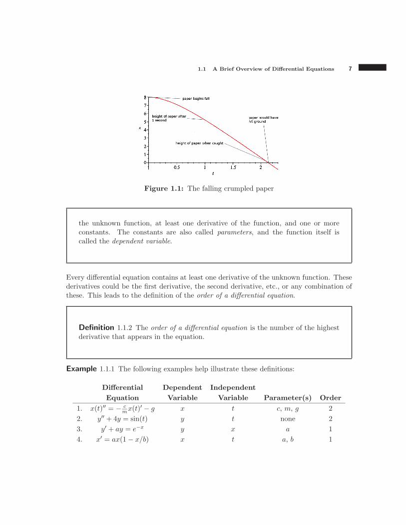
The entire process described above has taken the engineer only about a second (if youdoubt this is possible, just watch any episode of the television show “Numb3rs”). Thusshe still has time to save the ground from litter. She leans out the window and shouts toa bystander below, “Could you please catch that piece of paper for me?” At precisely 2.1seconds after the paper began its fall, and with just 0.026 seconds to spare, the bystanderreaches out and grabs the crumpled paper, thus saving the world from one more piece oflitter. See Figure 1.1 for a graphical visualization of this solution.
Terminology
We begin with a definition of a differential equation.
Definition 1.1.1 A differential equation (or DE for short) is an equation containingsome or all of the following: an unknown function, the independent variable of
1.1 A Brief Overview of Differential Equations 7
Figure 1.1: The falling crumpled paper
the unknown function, at least one derivative of the function, and one or moreconstants. The constants are also called parameters, and the function itself iscalled the dependent variable.
Every differential equation contains at least one derivative of the unknown function. Thesederivatives could be the first derivative, the second derivative, etc., or any combination ofthese. This leads to the definition of the order of a differential equation.
Definition 1.1.2 The order of a differential equation is the number of the highestderivative that appears in the equation.
Example 1.1.1 The following examples help illustrate these definitions:
Differential Dependent Independent
Equation Variable Variable Parameter(s) Order
1. x(t)′′ = − cmx(t)′ − g x t c, m, g 2
2. y′′ + 4y = sin(t) y t none 2
3. y′ + ay = e−x y x a 1
4. x′ = ax(1− x/b) x t a, b 1
8 CHAPTER 1 Introduction to Differential Equations
Notice that in equation 1, the independent variable is given along with the dependentvariable as x(t). In the other three equations, this is not the case. In equations 2 and 3, wemust use the context to determine which variable is which. In equation 4, no independentvariable is explicitly given. By convention, when the dependent variable is x, we typicallyuse t as the independent variable. When the dependent variable is y and no indpendentvariable is explicitly given, we typically use x as the dependent variable.
Solutions to Differential Equations
In the crumpled paper scenario we used the term solution to describe the function x(t) =−2.45 exp(−2t)− 4.9t+ 10.45. Now we define what we mean by a solution to a DE.
Definition 1.1.3 A solution to a DE is a function that when substituted into theDE for the dependent variable, results in a true statement (meaning both sides ofthe equation are the same) for all values of the independent variable.
It should be stressed that the substitution mentioned in this definition involves substitutingboth the function and its derivative(s) into the DE. Verifying that a claimed solution reallyis a solution to a DE simply involves calculating the appropriate derivatives, substituting,and simplifying, as illustrated in the next example.
Example 1.1.2 The crumpled paper scenario involved solving the DE
x′′ = −2x′ − 9.8
We claimed thatx(t) = −2.45 exp(−2t)− 4.9t+ 10.45
solves this differential equation. Verify that this is indeed a solution.
Solution: This DE involves both the first and second derivatives of x. First we calculatethese:
x′ = 4.9 exp(−2t)− 4.9
x′′ = −9.8 exp(−2t).
1.1 A Brief Overview of Differential Equations 9
Then we substitute these derivatives into the DE and verify that both sides really are equal:
−9.8 exp(−2t)?=−2 (4.9 exp(−2t)− 4.9)− 9.8
−9.8 exp(−2t)?=−9.8 exp(−2t) + 9.8− 9.8
−9.8 exp(−2t)=−9.8 exp(−2t).
Note that we put question marks over the equal signs because we are not sure that the twosides really are equal, until the last equation. Since this last equation is indeed true, weconclude that x(t) = −2.45 exp(−2t)− 4.9t+ 10.45 is a solution.
Verifying that a given function is a solution is relatively easy. Finding a solution is an-other issue. Sometimes, as illustrated in the next two examples, we can find a solution byreasoning with our knowledge of calculus and making educated guesses.
Example 1.1.3 Find a solution to the DE y′ = y.
Solution. Note that the differential equation expressed in words says “the derivative ofa function is equal to function you started with.” We should ask ourselves if we know offunction with this property. From calculus we know that the only function that is its ownderivative is the exponential function y = ex.
We now check our guess. The derivative of of y = ex is y′ = ex. Substituting ex in for bothy and y′ in the differential equation y′ = y we get
ex = ex,
which is clearly a true statement. This verifies our solution.
In the previous example, it may have been a surprise to see an exponential function appearas the solution to a differential equation that itself had no exponential function in it. Itis often the case that a solution to differential equations looks nothing like the DE fromwhich it came.
Example 1.1.4 Find a solution to the DE y′′ = −y.
Solution. In words, this DE says, “the second derivative of a function is equal to thenegative of the function.” We might consider the exponential function y = ex, but thisdoes not work this time, as its second derivative is ex, not −ex. To get a negative signinvolved, we might try y = e−x But then y′ = −e−x and y′′ = e−x which is the originalfunction and not the negative of it.

10 CHAPTER 1 Introduction to Differential Equations
So let’s consider something completely different. Consider the trigonometric function y =cos(x). Its first and second derivatives are
y′ = − sin(x) and y′′ = − cos(x).
Substituting these derivatives into the DE y′′ = −y we get − cos(x) = − cos(x), which is atrue statement. This verifies the solution. Similar calculations verify that y = sin(x) alsois a solution.
Comparison of algebraic equations and differential equations
A differential equation is an equation involving an uknown function. In the equationswe solved in high school algebra, the unknown was a number. Such equations are calledalgebraic equations. For example, the equation
2x+ 1 = 7
is an algebraic equation. To solve this equation, we “do the opposite of what is being doneto the unknown” by subtracting 1 from both sides, and then dividing by 2 to get x = 3. Tocheck this solution, we substitute 3 in for x in the equation 2x+ 1 = 7 to get 2(3) + 1 = 7,which is a true statement.
A solution to an algebraic equation is a number, whereas the solution to a differentialequation is a function. To check a solution both cases we substitute the claimed solutioninto the equation, and if we get a true statement then we have shown that the solutionis correct. With simple algebraic equations we may be able to guess the solution, but formore complicated ones we need algebra. Differential equations are similar. For very simpleDE’s, as the ones we encountered in the previous two examples, we were able to guess asolution. But more generally we will need some techniques (using calculus in addition toalgebra) for coming up with solutions. Throughout this text we will develop techniques fordoing just this.
Solving a DE problem can involve solving both DE’s and algebraic equations. Consider thecrumpled paper scenario. To find when the paper hit the ground, we first had to solve theDE
x′′ = −2x′ − 9.8,
and then we had to solve the algebraic equation
−2.45 exp(−2t)− 4.9t+ 10.45 = 0.
1.1 A Brief Overview of Differential Equations 11
In some cases, a DE can be converted into an algebraic equation which can then be solvedusing algebraic techniques (see Chapter 5). In this text we assume that the reader canobtain solutions to algebraic equations when needed, even when (as in the crumpled pa-per example) the solution cannot be obtained using standard algebraic techniques, usingavailable software as needed.
General solutions to first-order differential equations
When performing antiderivatives in calculus, we always have an arbitrary constant +C atthe end. For example, the general power rule is
∫
xndx =1
n+ 1xn+1 + C.
Students often think of the +C as a meaningless minor technicality. When solving DE’s,the +C is extremely important and cannot be ignored.
For example, consider the first order DE
y′ = 2x.
The unknown in this equation is the function y(x). To solve for y, we can use the generalprinciple for solving algebraic equations: Do the opposite of what is being done to theunknown. In this case, the derivative is being done to the unknown. The opposite of thederivative is the antiderivative, so we take the antiderivative of both sides of the equation:
∫
y′dx =
∫
2x dx ⇒ y = x2 + C.
Notice that we integrate with respect to x because this is the independent variable. Thisgives the explicit solution y = x2+C. Because this solution involves an arbitrary constant,this solution is called a general solution.
We can choose any value of the arbitrary constant and have a solution. For instance,
y = x2 + 1, y = x2 − 2.6, and y = x2,
corresponding to C = 1, −2.6, and 0, respectively, are all solutions to the DE y′ = 2x (thereader should verify this). These solutions are called particular solutions.
12 CHAPTER 1 Introduction to Differential Equations
Definition 1.1.4 A general solution of a first order DE is a solution with oneconstant that does not appear in the original differential equation. This is alsocalled a one-parameter family of solutions. When a particular value of the constantis chosen, we get a particular solution.
In some texts, the term general solution is reserved only for those situations where everypossible solution to the differential equation corresponds to some value of the arbitraryconstant. In this text, we use the term general solution in a slightly different way. Generalsolutions to higher-order equations and systems of equations will be discussed in laterchapters.
Not all general solutions involve a constant added to the end, as illustrated in the nextexample.
Example 1.1.5 Show that y = 2ex, y = −3ex, and y = 0 are all solutions to the DE y′ = yand find a general solution to this DE.
Solution. The derivatives of these claimed solutions are 2ex, −3ex, and 0, respectively.Notice that in each case, the derivative equals the function. Thus these are indeed solutions.
To find a general solution, note that all these solutions are of the form Cex where C is aconstant (in the solution y = 0, the constant is C = 0). Therefore, a general solution isy = Cex.
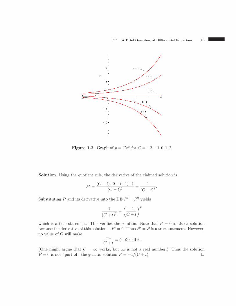
We can picture a general solution to a first-order differential equation by graphing thesolution for several values of the constant. Such graphs are called solution curves. Figure1.2 shows the solution curves to y′ = y corresponding to C = −2, −1, 0, 1, and 2.
The next example illustrates that a general solution does not always describe all of thesolutions to a DE.
Example 1.1.6 Show that a general solution to the differential equation P ′ = P 2 is
P =−1
C + t.
Also show that P = 0 is also a solution that does not correspond to any real value of C.
1.1 A Brief Overview of Differential Equations 13
Figure 1.2: Graph of y = Cex for C = −2,−1, 0, 1, 2
Solution. Using the quotient rule, the derivative of the claimed solution is
P ′ =(C + t) · 0− (−1) · 1
(C + t)2=
1
(C + t)2.
Substituting P and its derivative into the DE P ′ = P 2 yields
1
(C + t)2=
( −1
C + t
)2
which is a true statement. This verifies the solution. Note that P = 0 is also a solutionbecause the derivative of this solution is P ′ = 0. Thus P ′ = P is a true statement. However,no value of C will make −1
C + t= 0 for all t.
(One might argue that C = ∞ works, but ∞ is not a real number.) Thus the solutionP = 0 is not “part of” the general solution P = −1/(C + t).
14 CHAPTER 1 Introduction to Differential Equations
Initial value problems
The inclusion of an arbitrary constant in a general solution means a DE has infinitelymany solutions. Laplace’s dream includes the desire to predict the future with certainty.An infinite number of solutions means an inifite number of predictions. So how can wefulfill Laplace’s dream?
Laplace’s quote contains an additional idea that we have overlooked to this point. In parthe says,
An intellect which at a certain moment would know all forces that set nature inmotion, and all positions of all items of which nature is composed ... for suchan intellect nothing would be uncertain and the future just like the past wouldbe present before its eyes.
It’s the “all positions” part that we have not taken into account yet. Specifically, we havenot taken into account the starting positions. In terms of the DE, we have not taken intoaccount the value of the unknown function at the starting value of the independent variable.This condition is called an initial condition. So to predict the future, we need to know both
the differential equation and the initial conditions.
For a first-order differential equation, an initial condition consists of the value of the depen-dent variable given at some value of the independent variable. A DE along with an initialcondition is called an initial value problem. The initial condition is used to find the valueof the arbitrary constant, yielding a particular solution.
Example 1.1.7 We have shown that a general solution of the DE y′ = y is y = Cex.Suppose we are told that y = 3 when x = 0, that is y(0) = 3. Use this initial condition tofind a particular solution.
Solution. We substitute y = 3 and x = 0 into the general solution to get
3 = Ce0 = C,
which determines the value of C. Thus the particular solution is y = 3ex.
Initial value problems occur frequently in applications, as illustrated in the next example.
Example 1.1.8 (Population Dynamics) An important area of science that crosses severalacademic boundaries is the study of population growth. Mathematicians, biologists, ecol-ogists and others work together to create mathematical models that describe the growth
1.1 A Brief Overview of Differential Equations 15
of populations (animal, human, plant, microbial, etc.). Though such models may lack thepredictive precision of Newton’s second law, they can be very useful to scientists trying tomanage natural resources.
The simplest population model is based on the assumption that the rate of growth of thepopulation is proportional to the size of the population. This assumption is simply sayingthat large populations grow at a faster rate than small populations. If y(t) represents thenumber of organisms at time t, then this assumption yields the differential equation
y′ = ky
where k is a constant called the growth constant or growth rate.
Suppose a population of bacteria in a Petri dish grows according to this DE with growthconstant k = 3, where time t is in days and y(t) is measured in hundreds of bacteria.Suppose that there were initially 1,000 organisms in the dish. Show that y = Ce3t is ageneral solution of this DE, and use the initial condition to predict how many bacteriathere will be in 2 days.
Solution. To verify the general solution, note that its derivative is
y′ = 3Ce3t.
Substituting the claimed solution and its derivative into the DE y′ = 3y, we get 3Ce3t onboth sides, verifying that y = Ce3t is a general solution.
If we take the initial time to be t = 0, then the initial condition is y(0) = 10. To find C,we substitute t = 0 and y = 10 into y = Ce3t to get
10 = Ce3(0) = C,
which yields the particular solution y = 10e3t. This solution can be used to make predic-tions. After t = 2 days we predict that we will have
y = 10e3(2) ≈ 4034.3 thousand bacteria.
We must stress that such a prediction is at best an approximation, based on the assumptionthat the population is described by the DE y′ = 3y. If this assumption is not accurate,then our prediction is not accurate, regardless of the rigor of our mathematics.
16 CHAPTER 1 Introduction to Differential Equations
Higher order differential equations
Our discussion of general solutions, arbitrary constants, and initial conditions has so farbeen restricted to first-order differential equations. To summarize, for a first-order differ-ential equation, the general solution will contain one arbitrary constant, and we thereforeneed one initial condition in order to determine that constant.
In our discussion of general solutions of first-order DE’s, we saw that the arbitrary con-stant comes from integrating to “undo” the derivative. A second-order DE involves twoderivatives. So, informally, we will have to integrate twice to solve it. This results in twoarbitrary constants in a general solution. Finding the values of these constants requires theuse of two initial conditions. In general:
A general solution to an nth order DE will contain n arbitrary constants and willrequire n initial conditions to find a particular solution. These initial conditionscan be conditions on the value of the unknown function, or on the value(s) ofits derivative(s).
Example 1.1.9 In the crumpled paper scenario, we found a particular solution to thesecond-order DE x′′ = −2x′ − 9.8. Show that x(t) = −0.5C1e
−2t − 4.9t + C2 is a generalsolution to this DE. Then use the initial conditions x(0) = 8 and x′(0) = 0 to determineC1 and C2. Compare this result to the particular solution found by the engineer.
Solution. We take two derivatives of x(t) = −0.5C1e−2t − 4.9t+ C2 to get
x′(t) = C1e−2t − 4 and x′′(t) = −2C1e
−2t.
Substituting these into the DE x′′ = −2x′ − 9.8
−2C1e−2t = −2(C1e
−2t − 4.9)− 9.8,
which is a true statement. This verifies the general solution.
Next we use the initial condition x′(0) = 0 to find C1 by substituting t = 0 and x′ = 0 intox′(t) = C1e
−2t − 4.9:0 = C1 − 4.9 ⇒ C1 = 4.9.
Finally, we use the initial condition x(0) = 8 to find C2 by substituting t = 0, x = 8, andC1 = 4.9 into x(t) = −0.5C1e
−2t − 4.9t+ C2:
8 = −0.5(4.9) + C2 ⇒ C2 = 10.45.
1.1 A Brief Overview of Differential Equations 17
Thus the function that satisfies the differential equation and both initial conditions is
x(t) = −0.5(4.9)e−2t − 4.9t+ 10.45 = −2.45e−2t − 4.9t+ 10.45,
which is the same solution found by the engineer.
Systems of differential equations
Many real-world scenarios involve two or more unknown functions that “interact.” De-scribing these scenarios requires two or more DE’s. Such descriptions are called systems ofdifferential equations. A solution to a system of n DE’s consists of n functions which whensubstituted into the equations results in true statements.
Systems of first-order DE’s are important, in part, because an nth-order DE can be rewrittenas an equivalent system of n first-order DE’s. The system may be easier to solve than theoriginal single DE.
Example 1.1.10 The equations
x′ = y,
y′ = −x
form a system of two first-order differential equations. Show that the functions
x(t) = C1 cos(t) + C2 sin(t),
y(t) = −C1 sin(t) + C2 cos(t)
form a general solution to this system. In addition, find the particular solution satisfyingthe initial conditions x(0) = 1 and y(0) = −1.
Solution. The derivatives of these functions are
x′(t) = −C1 sin(t) + C2 cos(t),
y′(t) = −C1 cos(t)− C2 sin(t)
= −(C1 cos(t) + C1 sin(t)).
This shows that x′ = y and y′ = −x, and hence x(t) and y(t) form a general solution.
Substituting t = 0, x = 1, and y = −1 into the general solution for x(t) and y(t) we get
18 CHAPTER 1 Introduction to Differential Equations
the two equations
1 = C1 cos(0) + C2 sin(0),
−1 = −C1 sin(0) + C2 cos(0),
which simplify to C1 = 1 and C2 = −1. Thus
x(t) = cos(t)− sin(t),
y(t) = − sin(t)− cos(t)
is the particular solution.
In the previous example we were given a system of DE’s and enough initial conditions tofind the values of the constants in the general solution. This leads to our definition of aninitial value problem.
Definition 1.1.5 An initial value problem (or IVP for short) consists of a differ-ential equation or system of differential equations, along with a sufficient numberof initial conditions to determine the arbitrary constants in the general solution tothe differential equation. When there is more than one initial condition given, theymust all be given at the same value of the independent variable.
A solution to an initial value problem is a function which satisfies both the differ-ential equation(s) and the initial condition(s).
Example 1.1.11 Show that the given function is a solution to the given IVP.
Number Function(s) IVP
1. y = 3e10x y′ = 10y, y(0) = 3
2. y = 3 cos(t) y′′ + y = 0, y(0) = 3, y′(0) = 0
3. x = sin(t), y = cos(t) x′ = y, y′ = −x, x(0) = 0, x(0) = 1
Solution. Verifying a solution to an IVP requires verifying that the solution satisfies theDE and the initial conditions.
1.1 A Brief Overview of Differential Equations 19
Number Verify DE Verify IC
1. y′ = 30e10x = 10 · 3e10x = 10y y(0) = 3e10(0) = 3
2. Note that y′ = −3 sin(t) y(0) = 3 cos(0) = 3
and y′′ = −3 cos(t) y′(0) = −3 sin(0) = 0
so y′′ + y = −3 cos(t) + 3 cos(t) = 0.
3. x′ = cos(t) = y x(0) = 0
y′ = − sin(t) = −x y(0) = 1
Exercises
Directions: For each equation 1-6 below, determine its order. Also, name the independentvariable, the dependent variable, and any parameters in the equation. If it is not clear whatthe independent variable is, choose one (generally t or x if it is not being used as a dependentvariable). Assume any letters that are not t, x, or y are parameters.
1.1.1 y′ = ky
1.1.2 dP/dt = rP (1− P/N)
1.1.3 x′′ + 2x′ + 2x = sin(t)
1.1.4 θ′′ + θ′ + k sin θ = 0
1.1.5 d4ydx4 + 4y = 0
1.1.6 T ′(t) = k(A− T (t))
Guess a solution to each DE below. It does not have to be a general solution. Check yourguess to make sure that it works.
1.1.7 y′ = −y
1.1.8 y′ = −5y
1.1.9 y′′ = y
1.1.10 y′′ = 3y
1.1.11 y′′ = −3y
1.1.12 y(4) = y (here y(4) means the fourth derivative of y)
20 CHAPTER 1 Introduction to Differential Equations
For each of the equations, or system of equations below, show that the given function(s)form a solution.
1.1.13 Equation is y′ = y + 1, solution is y(t) = et − 1
1.1.14 Equation is y′ = y + sin(t), solution is y(t) = et − 12 sin t− 1
2 cos t
1.1.15 Equation is x′′ + 4x′ + 4x = 0, solution is x(t) = e−2t
1.1.16 Equation is x′′ + 4x′ + 4x = 0, solution is x(t) = te−2t
1.1.17 System is x′ = y, y′ = 4x , solution is x (t) = − 12e
−2t, y (t) = e−2t
1.1.18 System is x′ = y, y′ = 4x , solution is x (t) = 12e
2t, y (t) = e2t,
In each problem below, a differential equation, a general solution to the differential equationand one or more initial conditions are given. First show that the given function is in facta solution, then use the initial condition(s) to determine the (integration) constants.
1.1.19 Equation is y′ = y + 1, general solution is y(t) = Cet − 1, initial condition is y(0) = 4.
1.1.20 Equation is y′ = y+sin(t), general solution is y(t) = Cet − 12 sin t− 1
2 cos t, initial conditionis y(0) = 0.
1.1.21 Equation is x′′ − 4x = 0, general solution is x(t) = C1e−2t + C2e
2t, initial conditions arex(0) = 1, x′(0) = 0.
1.1.22 Equation is x′′+4x′+4x = 0, general solution is x(t) = C1e−2t+C2te
−2t, initial conditionsare x(0) = 1, x′(0) = 0.
1.1.23 System is x′ = y y′ = 4x , general solution is x (t) = 12C1e
2t − 12C2e
−2t, y (t) = C1e2t +
C2e−2t, initial conditions are x(0) = 1, y(0) = −1.
1.1.24 System is x′ = y y′ = −4x , general solution is x (t) = − 12C1 cos(2t)+
12C2 sin(2t), y (t) =
C1 sin(2t) + C2 cos(2t), initial conditions are x(0) = 1, y(0) = −1.
1.2 Explicit, Numerical, and Graphical Solutions
In Section 1.1 we defined a DE as an equation involving an unknown function and one ormore of its derivatives and a solution to a DE to be a function which, when substitutedinto the DE, results in a true statement for all values of the independent variable. So far wehave come up with an algebraic representation of a solution (a “formula” for the dependentvariable in terms of the independent variable), which we will refer to as an explicit solution.The problem is that for many DE’s, such an explicit solution cannot be found.
Solving a DE means finding the unknown function. There are three common ways ofrepresenting a function:
1.2 Explicit, Numerical, and Graphical Solutions 21
1. Algebraically (a “formula” for the function)
2. Numerically (a table of numerical outputs for different inputs)
3. Graphically (a plot of the outputs vs the inputs)
In cases where an explicit solution cannot be found, one can resort to approximation meth-ods that give either approximate values of the outputs for different inputs or an approxima-tion of the graph without having to find an explicit solution. The results are often referredto as numerical and graphical, or geometrical solutions, respectively.
In this section we define an explicit solution and describe some basic methods for findingnumerical and graphical solutions.
Explicit solutions and elementary functions
Before we define an explicit solution, we define elementary functions.
Definition 1.2.1 To say that an algebraic expression can be written in terms ofelementary functions means that the expression can be built from a finite numberof exponentials, logarithms, trigonometric functions and their inverses, constants,and nth roots through composition and combinations using the four elementaryoperations of addition, subtraction, multiplication, and division.
The next example illustrates this definition.
Example 1.2.1 The following algebraic expressions can be expressed in terms of elementaryfunctions:
sin(x)− x, 3 cos(2x),2√x+ ln(2x)
5ex − arctan(x2 + 2x+ 1), and 1.
The following cannot be expressed in terms of elementary functions:
erf(x) =2√π
∫ x
0e−t2dt, Γ(x) =
∫ ∞
0e−ttx−1dt, and
22 CHAPTER 1 Introduction to Differential Equations
Jα(x) =∞∑
m=0
(−1)m
m!Γ(m+ α+ 1)(1
2x)2m+α.
These last three functions are very important in mathematics, and have the names Error
function, Gamma function, and Bessel function (of the first kind), and are genericallyreferred to as special functions. It can be proven that these three functions cannot bewritten in terms of elementary functions, but the proofs are beyond the scope of thisbook.3
Elementary functions are the types of functions we are used to working with, and they arerelatively intuitive to understand. Our definition of an explicit solution involves elementaryfunctions.
Definition 1.2.2 An explicit solution to a differential equation or initial valueproblem is an algebraic representation of the solution to the DE or IVP, written interms of elementary functions, where the dependent variable is written explicitlyin terms of the independent variable.
Our definition of explicit solution is more restrictive than the way the term is used some-times in the literature. Some texts and articles allow the use of special functions in whatthey refer to as explicit solutions. In this text when when we say “explicit solution” wereally mean “explicit solution solution written in terms of elementary functions.” All of thesolutions found in the examples of Section 1.1 are explicit solutions.
Computer algebra systems
Computer algebra system (CAS) software such as Maple, Mathematica, Matlab, Maxima,some calculators such as the CAS enabled TI89, and websites such as Wolfram Alpha canfind explicit solutions to DE’s. If initial conditions are not provided the software will returna general solution.
3What is considered “elementary” and what is not is somewhat arbitrary. Things could change in thefuture. Mathematics is an evolving discipline, not a static one. Perhaps Bessel functions will become socommon in the future that they will be a button on every scientific calculator, just like sin or cos, and thatthey will then be classified as elementary.
1.2 Explicit, Numerical, and Graphical Solutions 23
Example 1.2.2 Use available software to find general solutions to the following differentialequations. Also, state whether or not each solution given qualifies as an explicit solutionby our definition.
1. y′ = y(1− y)
2. y′′ + y = sin(t)
3. y′ = y2 − t
Solution. The following results are those given by Wolfram Alpha. In all parts, c1 and c2denote arbitrary constants.
1. y(x) =ex
c1 + exis an explicit solution
2. y(t) = c2 sin(t) + c1 cos(t)−1
2t cos(t) is an explicit solution
3. y(t) =i t3/2
(
−c1J− 4
3
(
23 i t
3/2)
+ c1J 2
3
(
23 i t
3/2)
− 2J− 2
3
(
23 i t
3/2)
)
− c1J− 1
3
(
23 i t
3/2)
2t(
c1J− 1
3
(
23 i t
3/2)
+ J 1
3
(
23 i t
3/2)
)
is not an explicit solution because of the use of the function J , a Bessel function(see Example 1.2.1).
Note that other software may return something that looks very different, or no result atall. For part 3, for instance, the TI89 just returns the original DE, meaning that it cannotfind a solution.
The main point of Example 1.2.2 is that not all explicit solutions to DE’s can be expressed interms of elementary functions. An explicit solution given in terms of non elementary func-tions, such as in part 3, may be fine from a theoretical perspective, but such a descriptiondoes not provide much intuitive insight into the behavior of the solution.
A numerical approach: Euler’s method
In Example 1.1.8, we solved the initial value problem
DE : y′ = 3y
IC : y(0) = 10
24 CHAPTER 1 Introduction to Differential Equations
by first finding a general explicit solution to the DE, y = Ce3x, and then using the initialcondition to find the particular solution y = 10e3x (note that we changed the independentvariable from t to x). We then used this particular solution to predict the future value ofy.
Numerical methods allow us to predict future values of the function without ever havingto find an explicit solution. Euler’s method is a relatively simple numerical algorithm fordoing just this to IVP’s of the form
DE : y′ = f(x, y)
IC : y (x0) = y0.
The right-hand side of this DE simply means that y′ is given in terms of the independentvariable and/or the dependent variable. Euler’s method is based on three observations:
1. The solution to this IVP is a function which has a graph that goes through the point(x0, y0).
2. y′ is the slope of the tangent line of this graph.
3. f(x, y) gives a formula for the slope of the tangent line at any point (x, y) on thegraph.
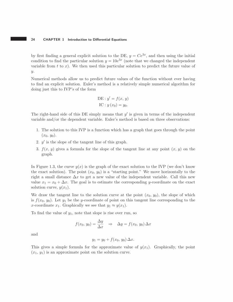
In Figure 1.3, the curve y(x) is the graph of the exact solution to the IVP (we don’t knowthe exact solution). The point (x0, y0) is a “starting point.” We move horizontally to theright a small distance ∆x to get a new value of the independent variable. Call this newvalue x1 = x0 +∆x. The goal is to estimate the corresponding y-coordinate on the exactsolution curve, y(x1).
We draw the tangent line to the solution curve at the point (x0, y0), the slope of whichis f(x0, y0). Let y1 be the y-coordinate of point on this tangent line corresponding to thex-coordinate x1. Graphically we see that y1 ≈ y(x1).
To find the value of y1, note that slope is rise over run, so
f(x0, y0) =∆y
∆x⇒ ∆y = f(x0, y0)∆x
andy1 = y0 + f(x0, y0)∆x.
This gives a simple formula for the approximate value of y(x1). Graphically, the point(x1, y1) is an approximate point on the solution curve.
1.2 Explicit, Numerical, and Graphical Solutions 25
Figure 1.3: First step of Euler’s method
Now take the new point (x1, y1) and use it as the starting point to find another new point(x2, y2) where
x2 = x1 +∆x,
y2 = y1 + f(x1, y1)∆x.
We can repeat this process as many times as we want to find any number of approximatepoints on the solution curve. We write the general algorithm as follows.
Euler’s Method for First-Order IVP’s
Given a differential equation y′ = f(x, y) and an initial condition y(x0) = y0,calculate the points (x1, y1) , . . . , (xn, yn) using
xi+1 = xi +∆x
yi+1 = yi + f(xi, yi)∆x
for i = 0, . . . , n− 1 where ∆x is a small positive number called the step size.
In problems such as Example 1.1.8, we want to know the value of y(b) where b is somegiven value of the independent variable. In such cases we can use the following relationship
26 CHAPTER 1 Introduction to Differential Equations
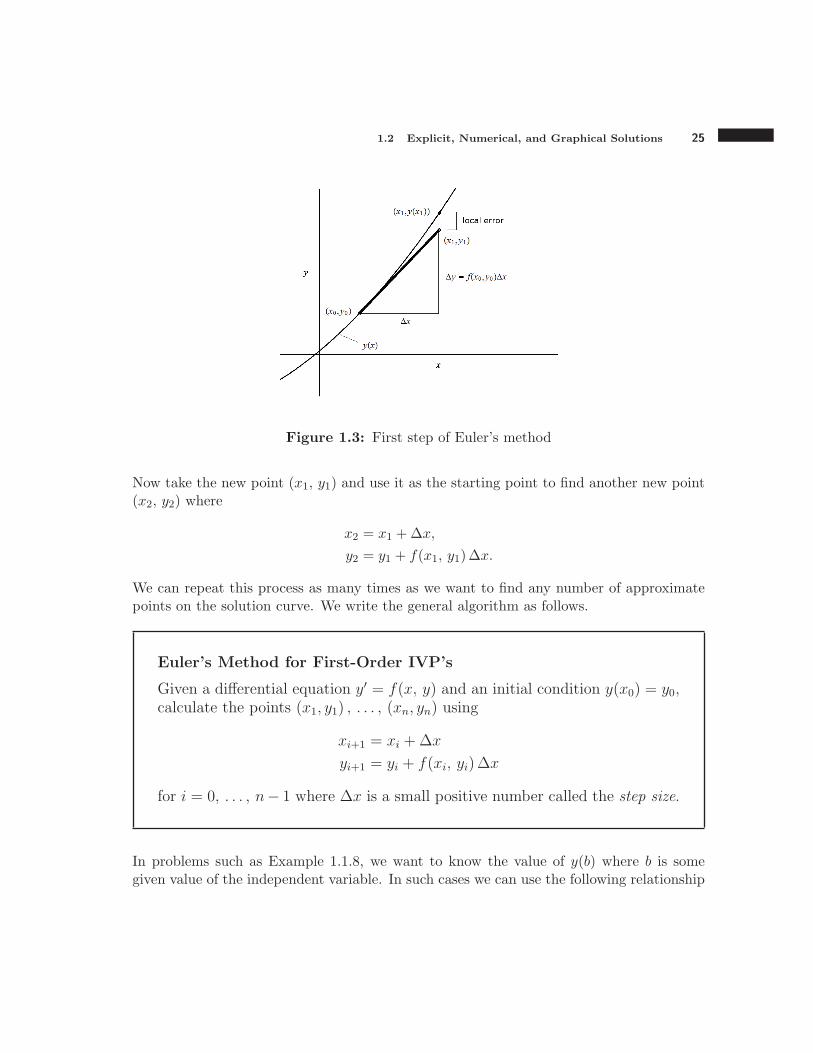
i xi yi f(xi, yi) = yi − xi yi+1 = yi + f(xi, yi)∆x
0 0 0.5 0.5− 0 = 0.5 0.5 + 0.5(0.5) = 0.75
1 0.5 0.75 0.75− 0.5 = 0.25 0.75 + 0.25(0.5) = 0.875
2 1.0 0.875 0.875− 1 = −0.125 0.875− 0.125(0.5) = 0.8125
3 1.5 0.8125 0.8125− 1.5 = −0.6875 0.8125− 0.6875(0.5) = 0.46875
4 2.0 0.46875
Table 1.1: Euler’s method for y′ = y − x
to find the necessary step size ∆x, or the number of steps n, given the other quantity:
∆x =b− x0
n.
Example 1.2.3 Consider the differential equation y′ = y − x with the initial conditiony(0) = 0.5. Use Euler’s method with step size ∆x = 0.5 to estimate y(2). Also useavailable software to find an explicit solution and use it to find the exact value of y(2).
Solution. We are given x0 = 0, b = 2, and ∆x = 0.5 so that the number of steps is
0.5 =2− 0
n⇒ n = 4.
We tabulate the values in Table 1.1. These calculations give y(2) ≈ 0.46875.
Wolfram Alpha gives the explicit solution y = C1ex+x+1. The initial condition y(0) = 0.5
yields 0.5 = C1 + 1 so that the particular solution is y = −0.5ex + x + 1. This gives theexact value
y(2) = −0.5e2 + 3 = −0.69453
accurate to five digits. In this case the Euler’s method approximation of y(2) is not verygood. In the next example we will see that we can greatly improve this approximation.
Figure 1.3 illustrates that yi is not quite equal to y(xi) (the exact value of the solution atx = xi). The error
| y(xi)− yi|for i = 0, . . . , n− 1 is called the local truncation error. When trying to estimate y(b) usingn steps, the error
| y(b)− yn|
1.2 Explicit, Numerical, and Graphical Solutions 27
is called the global truncation error. In Example 1.2.3 the Euler method estimate of y(2)using n = 4 steps was 1.46875 and the exact value of y(2) was −0.69453 to five digits. Theglobal truncation error is
|1.46875− (−0.69453)| = 2.1633.
This is a very large error. This error could be decreased by making the step size ∆x smaller.However, there is a trade-off. A smaller step size requires a larger number of steps. If wewere to choose a step size of ∆x = 0.1, the number of steps would be
0.1 =2− 0
n⇒ n = 20.
This number of calculations is impractical to do by hand, but luckily Euler’s method iseasy to implement on a computer. The issue of errors in Euler’s method will be discussedmore in Chapter 2.
Euler’s method with software
Euler’s method is an option when numerically solving initial value problems on the majorcomputer algebra systems, certain calculators, and many applets including those on theauthor’s website. These software calculate the points (x1, y1) , . . . , (xn, yn) and providethem in the form of a table. The software also plots the points and connects them withstraight lines to approximate the exact solution curve.
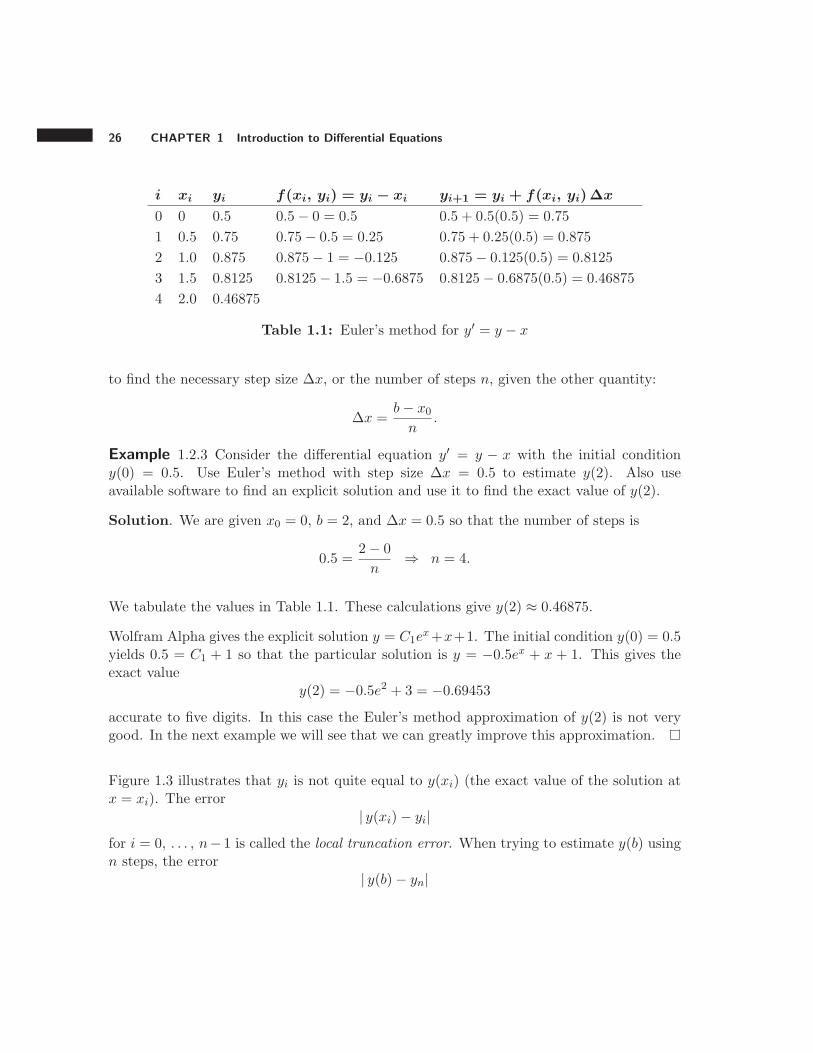
Example 1.2.4 Use available software, or the applet labeled Example 1.2.4 at uhaweb.
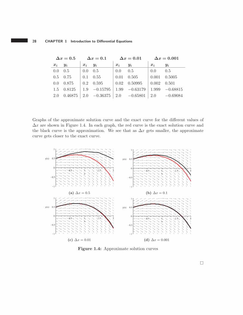
hartford.edu/rdecker/DeckerDEbook/DeckerDEbook.html to approximate the solutionthe differential equation y′ = y − x with the initial condition y(0) = 0.5 over the interval0 ≤ x ≤ 2 using step sizes of ∆x = 0.5, 0.1, 0.01, and 0.001. Compare these approximatesolutions to the exact solution y = −0.5ex + x + 1. What happens to the quality of theapproximations as ∆x gets smaller?
Solution. Partial tables of the results given by the applet referenced above are shownbelow. The exact value of y(2) is −0.69453. Notice that as ∆x gets smaller, the value ofyn gets closer to this exact value.
28 CHAPTER 1 Introduction to Differential Equations
∆x = 0.5 ∆x = 0.1 ∆x = 0.01 ∆x = 0.001
xi yi xi yi xi yi xi yi
0.0 0.5 0.0 0.5 0.0 0.5 0.0 0.5
0.5 0.75 0.1 0.55 0.01 0.505 0.001 0.5005
0.0 0.875 0.2 0.595 0.02 0.50995 0.002 0.501
1.5 0.8125 1.9 −0.15795 1.99 −0.63179 1.999 −0.68815
2.0 0.46875 2.0 −0.36375 2.0 −0.65801 2.0 −0.69084
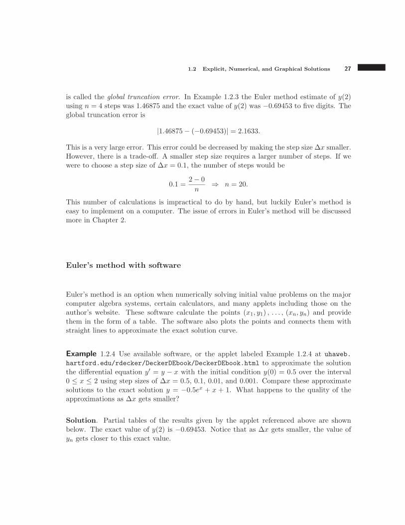
Graphs of the approximate solution curve and the exact curve for the different values of∆x are shown in Figure 1.4. In each graph, the red curve is the exact solution curve andthe black curve is the approximation. We see that as ∆x gets smaller, the approximatecurve gets closer to the exact curve.
(a) ∆x = 0.5 (b) ∆x = 0.1
(c) ∆x = 0.01 (d) ∆x = 0.001
Figure 1.4: Approximate solution curves
1.2 Explicit, Numerical, and Graphical Solutions 29
A geometrical approach: Slope Fields
Euler’s method is a fairly simple algorithm. But it has a drawback: it requires an initialcondition and thus gives us an approximation of a particular solution to the DE. In somecases we don’t know an IC, or we would like to know the behavior of the solution fordifferent IC’s. In otherwords, we would like a description of a general solution.
The method of slope fields allows us to visualize all possible solution curves to a differentialequation. That it, it gives us a graphical representation of a general solution. This methodapplies to first-order DE’s of the form
y′ = f(x, y)
but no initial condition is required. The key idea is the same as for Euler’s method: theright-hand side of the DE provides a formula for the slope of the solution curve at any givenpoint. The basic steps are as follows:
1. Choose a rectangular array of points in some region of the xy-plane.
2. At each point in the array, (x, y), calculate the slope of the solution curve, f(x, y).
3. At each point, sketch a small straight line with the associated slope. These lines arecalled slope marks. The resulting graph is called a slope field.
4. Sketch approximate solution curves by drawing curves that are approximately tangentto each slope mark the curve passes near.
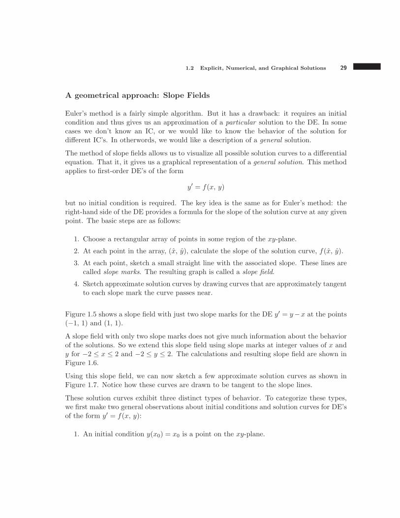
Figure 1.5 shows a slope field with just two slope marks for the DE y′ = y−x at the points(−1, 1) and (1, 1).
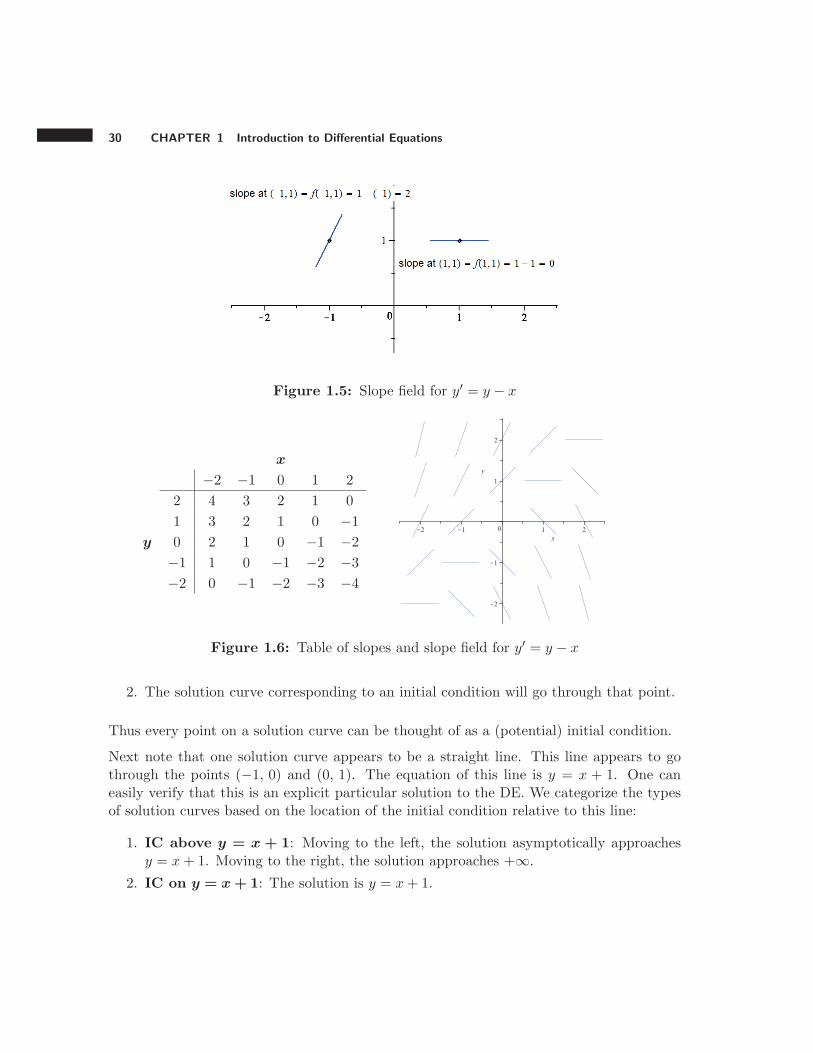
A slope field with only two slope marks does not give much information about the behaviorof the solutions. So we extend this slope field using slope marks at integer values of x andy for −2 ≤ x ≤ 2 and −2 ≤ y ≤ 2. The calculations and resulting slope field are shown inFigure 1.6.
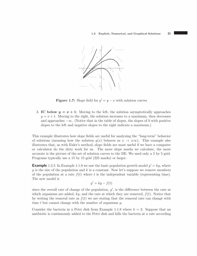
Using this slope field, we can now sketch a few approximate solution curves as shown inFigure 1.7. Notice how these curves are drawn to be tangent to the slope lines.
These solution curves exhibit three distinct types of behavior. To categorize these types,we first make two general observations about initial conditions and solution curves for DE’sof the form y′ = f(x, y):
1. An initial condition y(x0) = x0 is a point on the xy-plane.
30 CHAPTER 1 Introduction to Differential Equations
Figure 1.5: Slope field for y′ = y − x
x
−2 −1 0 1 2
2 4 3 2 1 0
1 3 2 1 0 −1
y 0 2 1 0 −1 −2
−1 1 0 −1 −2 −3
−2 0 −1 −2 −3 −4
Figure 1.6: Table of slopes and slope field for y′ = y − x
2. The solution curve corresponding to an initial condition will go through that point.
Thus every point on a solution curve can be thought of as a (potential) initial condition.
Next note that one solution curve appears to be a straight line. This line appears to gothrough the points (−1, 0) and (0, 1). The equation of this line is y = x + 1. One caneasily verify that this is an explicit particular solution to the DE. We categorize the typesof solution curves based on the location of the initial condition relative to this line:
1. IC above y = x + 1: Moving to the left, the solution asymptotically approachesy = x+ 1. Moving to the right, the solution approaches +∞.
2. IC on y = x+ 1: The solution is y = x+ 1.
1.2 Explicit, Numerical, and Graphical Solutions 31
Figure 1.7: Slope field for y′ = y − x with solution curves
3. IC below y = x + 1: Moving to the left, the solution asymptotically approachesy = x+ 1. Moving to the right, the solution increases to a maximum, then decreasesand approaches −∞. (Notice that in the table of slopes, the slopes of 0 with positiveslopes to the left and negative slopes to the right indicate a maximum.)
This example illustrates how slope fields are useful for analyzing the “long-term” behaviorof solutions (meaning how the solution y(x) behaves as x → ±∞). This example alsoillustrates that, as with Euler’s method, slope fields are most useful if we have a computeror calculator do the dirty work for us. The more slope marks we calculate, the moreaccurate is the picture of the set of solution curves to the DE. We used only a 5 by 5 grid.Programs typically use a 15 by 15 grid (225 marks) or larger.
Example 1.2.5 In Example 1.1.8 we saw the basic population growth model y′ = ky, wherey is the size of the population and k is a constant. Now let’s suppose we remove membersof the population at a rate f(t) where t is the independent variable (representing time).The new model is
y′ = ky − f(t)
since the overall rate of change of the population, y′, is the difference between the rate atwhich organisms are added, ky, and the rate at which they are removed, f(t). Notice thatby writing the removal rate as f(t) we are stating that the removal rate can change withtime t but cannot change with the number of organisms y.
Consider the bacteria in a Petri dish from Example 1.1.8 where k = 3. Suppose that anantibiotic is continuously added to the Petri dish and kills the bacteria at a rate according
32 CHAPTER 1 Introduction to Differential Equations
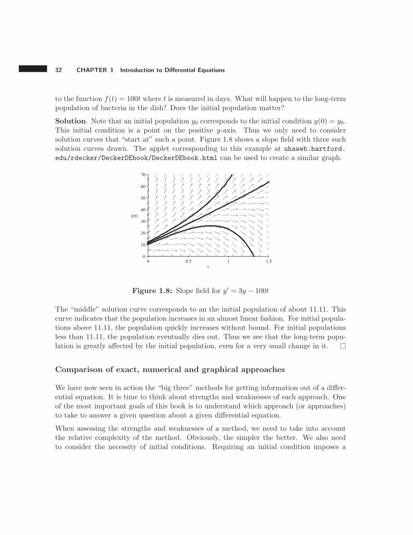
to the function f(t) = 100t where t is measured in days. What will happen to the long-termpopulation of bacteria in the dish? Does the initial population matter?
Solution. Note that an initial population y0 corresponds to the initial condition y(0) = y0.This initial condition is a point on the positive y-axis. Thus we only need to considersolution curves that “start at” such a point. Figure 1.8 shows a slope field with three suchsolution curves drawn. The applet corresponding to this example at uhaweb.hartford.
edu/rdecker/DeckerDEbook/DeckerDEbook.html can be used to create a similar graph.
Figure 1.8: Slope field for y′ = 3y − 100t
The “middle” solution curve corresponds to an the initial population of about 11.11. Thiscurve indicates that the population increases in an almost linear fashion. For initial popula-tions above 11.11, the population quickly increases without bound. For initial populationsless than 11.11, the population eventually dies out. Thus we see that the long-term popu-lation is greatly affected by the initial population, even for a very small change in it.
Comparison of exact, numerical and graphical approaches
We have now seen in action the “big three” methods for getting information out of a differ-ential equation. It is time to think about strengths and weaknesses of each approach. Oneof the most important goals of this book is to understand which approach (or approaches)to take to answer a given question about a given differential equation.
When assessing the strengths and weaknesses of a method, we need to take into accountthe relative complexity of the method. Obviously, the simpler the better. We also needto consider the necessity of initial conditions. Requiring an initial condition imposes a
1.2 Explicit, Numerical, and Graphical Solutions 33
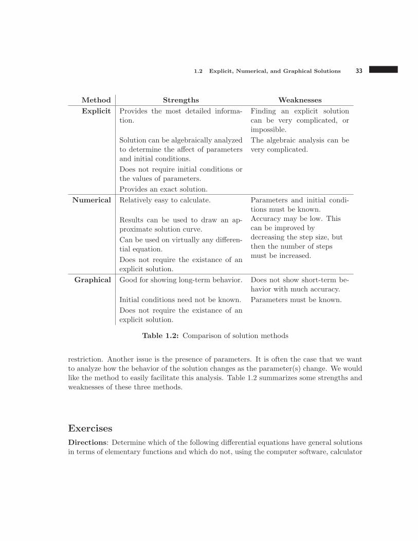
Method Strengths Weaknesses
Explicit Provides the most detailed informa-tion.
Finding an explicit solutioncan be very complicated, orimpossible.
Solution can be algebraically analyzedto determine the affect of parametersand initial conditions.
The algebraic analysis can bevery complicated.
Does not require initial conditions orthe values of parameters.
Provides an exact solution.
Numerical Relatively easy to calculate. Parameters and initial condi-tions must be known.
Results can be used to draw an ap-proximate solution curve.
Accuracy may be low. Thiscan be improved bydecreasing the step size, butthen the number of stepsmust be increased.
Can be used on virtually any differen-tial equation.
Does not require the existance of anexplicit solution.
Graphical Good for showing long-term behavior. Does not show short-term be-havior with much accuracy.
Initial conditions need not be known. Parameters must be known.
Does not require the existance of anexplicit solution.
Table 1.2: Comparison of solution methods
restriction. Another issue is the presence of parameters. It is often the case that we wantto analyze how the behavior of the solution changes as the parameter(s) change. We wouldlike the method to easily facilitate this analysis. Table 1.2 summarizes some strengths andweaknesses of these three methods.
Exercises
Directions: Determine which of the following differential equations have general solutionsin terms of elementary functions and which do not, using the computer software, calculator
34 CHAPTER 1 Introduction to Differential Equations
or website of your choice. Give the solution when you can find one.
1.2.1 y′ = y + sin(x)
1.2.2 y′ = x+ sin(y)
1.2.3 y′ + y = et
1.2.4 y′ + y3 = et
Use Euler’s method for each of the following. If more than 5 steps are required, use acomputer or calculator. If an exact solution is possible, find it, and calculate the error inEuler’s method.
1.2.5 Given that y′ = 3y − 100t and y(0) = 10, estimate y(1) using ∆t = 0.25.
1.2.6 Given that y′ = 3y − 100t and y(0) = 10, estimate y(1) using ∆t = 0.01.
1.2.7 Given that y′ = 3y(1− y100 )− 100t and y(0) = 10, estimate y(1) using ∆t = 0.25.
1.2.8 Given that y′ = 3y(1− y100 )− 100t and y(0) = 10, estimate y(1) using ∆t = 0.01.
Create slope fields as directed for each of the following DE’s. Sketch in a few solutioncurves based on the slope field. If more than 10 slope marks are required, use a computeror calculator. What can you say about the long term behavior of the differential equation(what happens for various initial conditions)?
1.2.9 DE is y′ = −2y, using integer values of the variables for 0 ≤ x ≤ 2 and −1 ≤ y ≤ 1.
1.2.10 DE is y′ = −2x, using integer values of the variables for 0 ≤ x ≤ 2 and −1 ≤ y ≤ 1.
1.2.11 DE is y′ = y(1− y) for −1 ≤ x ≤ 5 and −1 ≤ y ≤ 2 using a 15 by 15 grid or larger.
1.2.12 DE is y′ = y2 − t for −1 ≤ t ≤ 5 and −2 ≤ y ≤ 2 using a 15 by 15 grid or larger.
For each situation below, use whatever approach (exact, numerical, graphical) you feel ismost appropriate to answer the given question. When using a numerical approach useEuler’s method with step size 0.01. Use a computer algebra system (software, calculatoror website) to determine an exact solution if there is one.
1.2.13 A cup of coffee at 1800F is left in a room at 700F . Newton’s law of cooling states that therate of change of the temperature of an object is proportional to the difference between the object’stemperature and the surrounding (ambient) temperature. Letting y represent the temperature ofthe coffee and letting t represent time (in, say, minutes) we get the differential equation y′ = k(70−y)where k is the proportionality constant. The initial condition is y(0) = 180.
Assume that from experiment it has been found that for a cup of coffee, we have approximatelyk = 0.05. Find both the temperature after 10 minutes and the long-term temperature (that is, thetemperature after a very long time, that is, limt→∞ y(t) ).
1.3 Mathematical Modeling with Differential Equations 35
1.2.14 For the situation in problem 13, suppose we are interested in what happens to cups of coffeethat start out at various temperatures (not just 1800F )? Describe what happens to cups of coffeethat start out at any temperature ranging between 00F and 2000F . Give a qualitative descriptionfor the short term, and a more quantitative description (numerical values) for what happens in thelong term.
1.2.15 Recall the falling crumpled paper from Section 1.1. We made the assumption that the airresistance force was proportional to the velocity of the object, and we ended up with the differentialequation x′′ = −2x′ − 9.8. This assumption may be inaccurate for some objects. A more generalmodel for falling objects is x′′ = −k(x′)p−9.8 where we assume that the force due to air resistance isproportional to the velocity raised to some power of the velocity. Switching the dependent variableto velocity v = x′ we get v′ = −kvp − 9.8.
Assume that k = 2 as before, but now assume that p = 1.5 (instead of p = 1). The DE is nowv′ = −2v1.5 − 9.8. If the paper starts out at 0 velocity, estimate the velocity after 1 second. Alsodetermine the velocity after a long period of time (called the terminal velocity).
1.2.16 Find a linear function of the form f(t) = a+ bt that is a solution to the differential equationy′ = 3y − 100t. To do this substitute f(t) in for y in the differential equation and solve for theconstants a and b. This is one of the standard techniques of differential equations; assume a formfor the solution which contains arbitrary constants, substitute the proposed solution into the DE,then solve for the constants. Key idea: equate coefficients of like terms (with a polynomial the liketerms are the t0 terms, the t1 terms, the t2 terms and so on).
1.3 Mathematical Modeling with Differential Equations
We have used the term “model” several times in the first two sections of this text. In thissection we discuss what we mean by a model, some basic principles for constructing models,and a few examples of models.
We begin with a definition.
Definition 1.3.1 A mathematical model is a mathematical description of a real-world problem.
Mathematical models can take many forms. A model may be an algebraic equation, adifferential equation, a system of equations, an algorithm, a simulation, or any other number
36 CHAPTER 1 Introduction to Differential Equations
of possibilities. Differential equations are often used to construct models because it isoften easier to describe the way a quantity changes than it is to describe the quantityitself. Because of this, differential equations is one of the most applied branches in all ofmathematics.
Mathematical modeling is all about using mathematics to describe real-world problems.The mathematics world is very precise, rigorous, and certain. None of this is true aboutthe real world. Because of this, it is necessary to make assumptions about the way thereal-world works in order to construct a model. Every mathematical model is based onsome set of assumptions. The results of the model are only as valid as the assumptions onwhich it is based. This point cannot be over-stated.
Many mathematical models combine “laws of nature,” which have been extensively exper-imentally verified, and assumptions which may seem reasonable, but often do not have thepredictive accuracy of the laws of nature.
Example 1.3.1 In Section 1.1 we derived the DE mx′′ = −cx′ − mg to model a fallingcrumpled paper. This DE is an example of a mathematical model.
We derived this equation using two main ideas:
1. Newton’s second law∑
F = ma, which is a law of nature, and
2. the assumption that the force due to air resistance is proportional to the velocity.
A solution to this DE (whether explicit, numerical, or graphical) is only as valid as thisassumption. If the force due to air resistance behaves much differently than we think, thenour solution is invalid, regardless of the rigor of our mathematics.
Simplicity and Proportionality
One over-arching goal when creating mathematical models is to keep them simple. We oftenstart with the simplest possible model that has the potential to explain a given phenomena.If the predictions of the model are not sufficiently accurate for the application, then amore detailed model can be developed. This is essentially a variation of a philosophicalprinciple called Occam’s Razor, which states that among competing explanations of a givenphenomena, one should choose the simplest one.
One way to help keep a model simple is to simplify the description of the relationshipbetween two variables. Proportionality is often used to do just this.
1.3 Mathematical Modeling with Differential Equations 37
Definition 1.3.2 Two variables x and y are said to be directly proportional, orsimply proportional, if there exists a constant c 6= 0, called the constant of propor-
tionality such thaty = cx.
The variables are said to be inversely proportional if
y =c
x.
Two important observations need to be made:
1. If x and y are directly proportional, and c > 0, then if one variable increases, so doesthe other.
2. If x and y are inversely proportional, and c > 0, then if one variable increases, theother decreases.
In the crumpled paper scenario of Section 1.1, we modeled the force due to air resistance asproportional to the velocity. Hopefully this seems reasonable because if velocity increases,then the force due to air resistance will also increase. Granted, proportionality may not bethe only way of modeling this relationship, but it is the simplest.
Example 1.3.2 One famous law of nature involving inverse proportionality is Newton’slaw of universal gravitation. This law relates the distances between two objects with thegravitational force between them. In mathematical terms, this law states
F = Gm1m2
r2
where m1 and m2 are the masses, r is the distance between them, and G is the propor-tionality constant, called the gravitational constant. In words, this law states that F isinversely proportional to r2, meaning that as the distance between two objects increases,the gravitational force decreases. This relationship agrees with our intuition.
Another well-known mathematical model involving proportionality is Newton’s law of cool-
ing.
38 CHAPTER 1 Introduction to Differential Equations
Example 1.3.3 (Newton’s law of cooling) Consider the following observation:
A hot cup of coffee sitting on a desk initially cools very quickly. As its temper-ature approaches room temperature, the coffee cools much slower.
This observation can be used to model the temperature of the coffee at any point in time.If we let T (t) represent the temperature at time t and A represent the ambient tempera-ture (which we will assume is constant), then this observation suggests the following tworelationships:
1. When the difference between the ambient temperature and the temperature of thecoffee, (A− T ), is large, then the change in T , dT
dt is large.
2. When the difference is small, then the change is small.
These relationships suggest that dTdt is directly proportional to (A−T ). This yields the DE
dT
dt= k(A− T )
where k > 0 is a constant. This DE is known as Newton’s law of cooling. It can be used todescribe the temperature of a hot object cooling, or a cool object warming.
If A and T are measured in ◦F and t is measured in minutes, then the units on the left sideof the DE would be
◦Fmin and the units of (A− T ) would be ◦F. Thus to make the units on
both sides of the DE agree, the units of k would need to be min−1. The constant k can beinterpreted as a measure of how quickly the object cools (or warms).
Note that if A < T , meaning that the object is warmer than ambient temperature, then(A− T ) < 0. Thus dT
dt < 0 and the object’s temperature would be decreasing towards the
ambient temperature. Conversely, if A > T then dTdt > 0 so the object’s temperature would
increase towards the ambient temperature. This observation agrees with our intuition.4
Figure 1.9 shows a slope field along with several solution curves for the case A = 50◦F,k = 0.7. As intended, objects starting out with temperature less than 50◦F warm up untilthey reach 50◦F, and objects that start out with temperature greater than 50◦F cool untilthey reach 50◦F.
4Note that if we had constructed the model as dT
dt= k(T − A), then for this observation to be true we
would need k < 0. This would complicate the model. We prefer the simpler option.
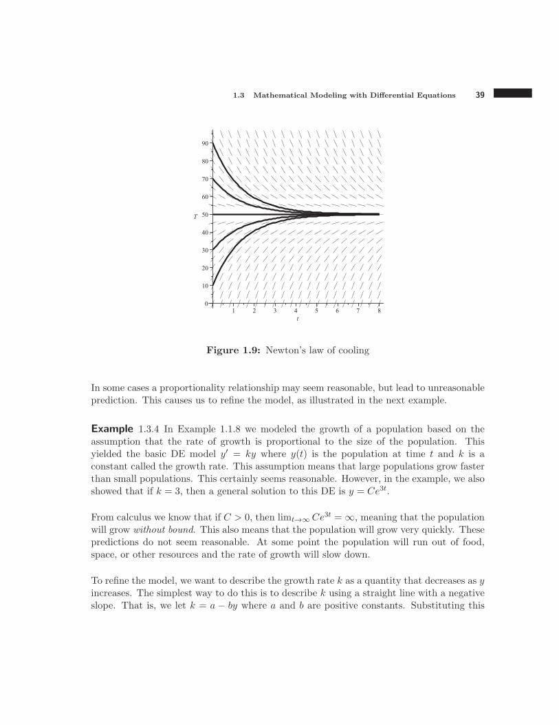
1.3 Mathematical Modeling with Differential Equations 39
Figure 1.9: Newton’s law of cooling
In some cases a proportionality relationship may seem reasonable, but lead to unreasonableprediction. This causes us to refine the model, as illustrated in the next example.
Example 1.3.4 In Example 1.1.8 we modeled the growth of a population based on theassumption that the rate of growth is proportional to the size of the population. Thisyielded the basic DE model y′ = ky where y(t) is the population at time t and k is aconstant called the growth rate. This assumption means that large populations grow fasterthan small populations. This certainly seems reasonable. However, in the example, we alsoshowed that if k = 3, then a general solution to this DE is y = Ce3t.
From calculus we know that if C > 0, then limt→∞Ce3t = ∞, meaning that the populationwill grow without bound. This also means that the population will grow very quickly. Thesepredictions do not seem reasonable. At some point the population will run out of food,space, or other resources and the rate of growth will slow down.
To refine the model, we want to describe the growth rate k as a quantity that decreases as yincreases. The simplest way to do this is to describe k using a straight line with a negativeslope. That is, we let k = a − by where a and b are positive constants. Substituting this
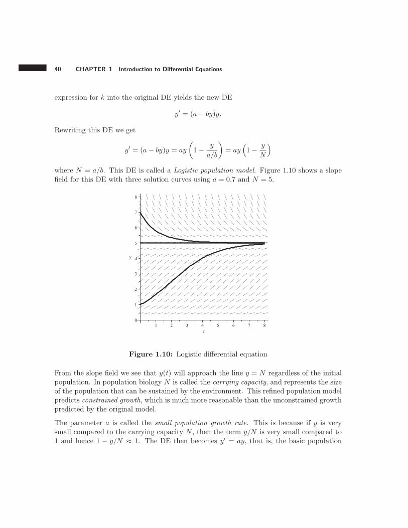
40 CHAPTER 1 Introduction to Differential Equations
expression for k into the original DE yields the new DE
y′ = (a− by)y.
Rewriting this DE we get
y′ = (a− by)y = ay
(
1− y
a/b
)
= ay(
1− y
N
)
where N = a/b. This DE is called a Logistic population model. Figure 1.10 shows a slopefield for this DE with three solution curves using a = 0.7 and N = 5.
Figure 1.10: Logistic differential equation
From the slope field we see that y(t) will approach the line y = N regardless of the initialpopulation. In population biology N is called the carrying capacity, and represents the sizeof the population that can be sustained by the environment. This refined population modelpredicts constrained growth, which is much more reasonable than the unconstrained growthpredicted by the original model.
The parameter a is called the small population growth rate. This is because if y is verysmall compared to the carrying capacity N , then the term y/N is very small compared to1 and hence 1 − y/N ≈ 1. The DE then becomes y′ = ay, that is, the basic population
1.3 Mathematical Modeling with Differential Equations 41
model, with growth rate a.
Balance of Units
When creating a model, we must be careful about units as stated in the following principle:
The units on both sides of a DE must always agree.
This principle helps to explain the necessity of a constant of proportionality and its meaningas illustrated in the next example.
Example 1.3.5 Suppose we tried to model a population of bacteria in a Petri disk withthe DE y′ = y where y represents the number of bacteria time is measured in hours. Theunits on the left-hand side would be bacteria per year and the units on the right would bebacteria. These units don’t agree. One way to solve this problem is to introduce a constantk in the model to get y′ = ky where k has the units hours−1.
So what does this constant k represent in a practical sense? We can rewrite this DE as
k =y′
y
which illustrates that k represents the net growth rate of the population per unit of popu-lation.
To further illustrate this interpretation, suppose the population were increasing at a rateof 100 bacteria per hour when there are 1000 bacteria in the dish, then
k =100
1000= 0.10
and the units of k would be
bacteria/hour
bacteria=
1
hours= hours−1
which are called “reciprocal hours.” What does this mean? Think in percentage terms.The value k = 0.10 indicates that each bacteria produces 0.10 bacteria per hour, meaningthe bacteria are increasing at a rate of 10% per hour. Thus whatever the value of k, itrepresents a 100k% net growth rate. It could also be interpreted as the difference betweenthe birth rate and the death rate.
42 CHAPTER 1 Introduction to Differential Equations
Approximating discrete variables with continuous ones
Variables representing quantities such as population can only take whole number values.Variables representing quantities such as mass do not have to take whole number values.This observation leads to the following definition.
Definition 1.3.3 A variable is said to be continuous if it can take any value withinsome interval. A variable is discrete if its set of possible values is finite or countable.
Informally, a variable is discrete if there are “gaps” between consecutive values. A variableis continuous if there are no gaps. Often when modeling with DE’s we approximate dis-crete variables with continuous ones. This can greatly simply our model because modelingdiscrete variables exactly can be very complicated.
In Example 1.3.5, the dependent variable y represents a population, which must be a wholenumber, so y is discrete. However, we described y with the DE y′ = ky. When we workwith the derivative of y, we are treating y as a continuous variable. In other words, weapproximated a discrete variable with a continuous one.
We must keep this approximation in mind when we interpret the results of the model. Ifthe model were to predict, say y(5) = 24.6, this would not mean there will be exactly 24.6bacteria at time 5. We would interpret this as meaning there would be about 24 or 25bacteria at time 5.
An approximation such as this tends to work best when the gaps between consecutivevalues of the dependent variable is small compared to possible values of the variable. Forexample, if time is our independent variable, and the population of the United States is ourdependent variable, then the gaps between consecutive values is 1, which is rather smallcompared to populations in excess of 300 million.
Note that in Example 1.3.5, the independent variable representing time in hours is contin-uous. In DE’s, the independent variable must be continuous in order for the derivative ofthe unknown function to exist. In some practical applications, both the independent anddependent variables are discrete. The next example illustrates such a scenario.
Example 1.3.6 The ring-tailed lemur has about a one month breeding season which runsfrom mid April to mid May, and the young are usually born in September. Let yi represent
1.3 Mathematical Modeling with Differential Equations 43
the number of lemurs in a population of lemurs at the beginning of year i, where i =0, 1, 2, ... Note that both the independent variable i and dependent variable yi are discrete.
We can model this scenario with a discrete logistic model
yi+1 = yi + ayi
(
1− yiN
)
(1.3)
where a is a constant and N is the carrying capacity. In words, this model says that thepopulation in the next year, yi+1, is equal to the population in the current year, yi, plusa fraction of the current population. As the current population gets closer to the carryingcapacity, this fraction gets closer to 0. Hopefully this model makes intuitive sense.
To illustrate how this model can be used to predict populations, suppose N = 100, a = 0.4,and y0 = 50. Then y1 is
y1 = 50 + (0.4)(50)(1− 50/100) = 60.0
and y2 isy2 = 60 + (0.4)(60)(1− 60/100) = 69.6.
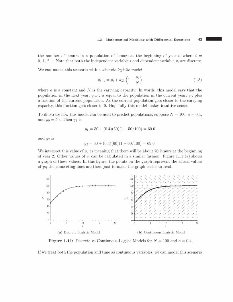
We interpret this value of y2 as meaning that there will be about 70 lemurs at the beginningof year 2. Other values of yi can be calculated in a similar fashion. Figure 1.11 (a) showsa graph of these values. In this figure, the points on the graph represent the actual valuesof yi; the connecting lines are there just to make the graph easier to read.
(a) Discrete Logistic Model (b) Continuous Logistic Model
Figure 1.11: Discrete vs Continuous Logisic Models for N = 100 and a = 0.4
If we treat both the population and time as continuous variables, we can model this scenario
44 CHAPTER 1 Introduction to Differential Equations
with the continuous logistic model
y′ = ay(
1− y
N
)
.
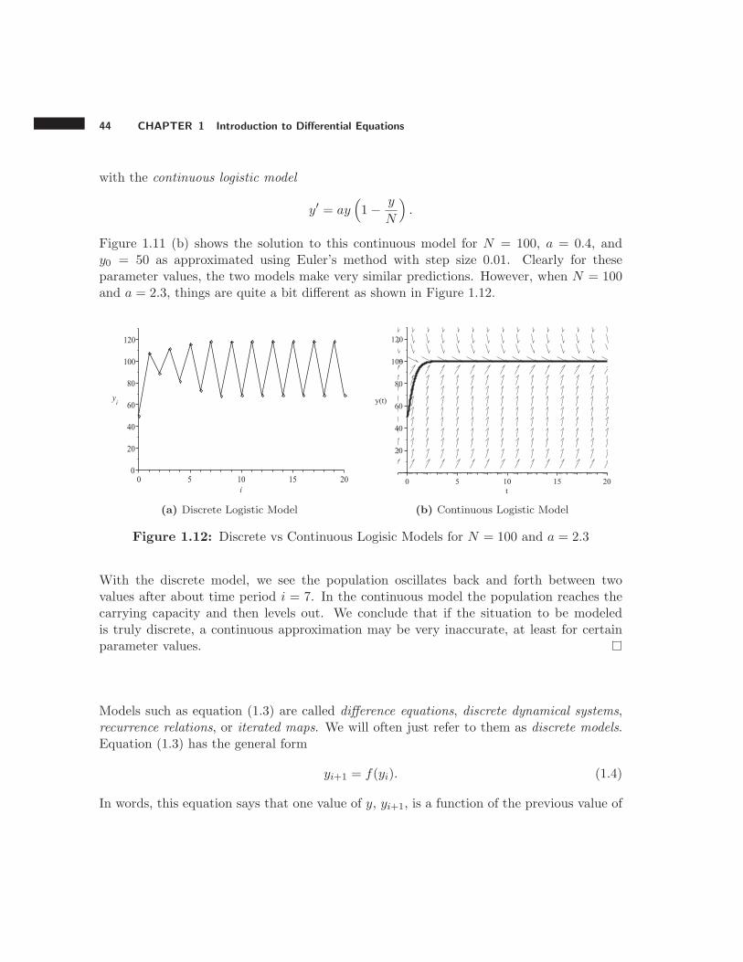
Figure 1.11 (b) shows the solution to this continuous model for N = 100, a = 0.4, andy0 = 50 as approximated using Euler’s method with step size 0.01. Clearly for theseparameter values, the two models make very similar predictions. However, when N = 100and a = 2.3, things are quite a bit different as shown in Figure 1.12.
(a) Discrete Logistic Model (b) Continuous Logistic Model
Figure 1.12: Discrete vs Continuous Logisic Models for N = 100 and a = 2.3
With the discrete model, we see the population oscillates back and forth between twovalues after about time period i = 7. In the continuous model the population reaches thecarrying capacity and then levels out. We conclude that if the situation to be modeledis truly discrete, a continuous approximation may be very inaccurate, at least for certainparameter values.
Models such as equation (1.3) are called difference equations, discrete dynamical systems,recurrence relations, or iterated maps. We will often just refer to them as discrete models.Equation (1.3) has the general form
yi+1 = f(yi). (1.4)
In words, this equation says that one value of y, yi+1, is a function of the previous value of

1.3 Mathematical Modeling with Differential Equations 45
y, yi. Now recall Euler’s method from Section 1.2 which was described with the equations
xi+1 = xi +∆x
yi+1 = yi + f(xi, yi)∆x.
Note that the equation for yi+1 is of the same general form as equation (1.4). Thus Euler’smethod is really a way of approximating a DE with a discrete model.
Rate of accumulation
Many scenarios involve a quantity that is being both increased and decreased. We candescribe the overall rate of change of this quantity with a basic modeling principle. Tomotivate this principle, consider the following scenario:
If you are rolling bowling balls down a lane at a rate of 10 per minute, andthe balls are coming back to you at a rate of 8 per minute, then there is apile of bowling balls somewhere growing larger at a rate of 2 per minute. Manyphysicists call this the “law of conservation of bowling balls,” though some insiston the more formal “law of conservation of matter.”
In more mathematical terms, we can describe this principle as
Rate of accumulation = Rate in − Rate out.
Our first application of this principle involves the idea of a concentration. The concentrationof a material in a solution is defined as
Concentration =Total amount of material in the solution
Total volume of the solution.
The material could be a solid, such as salt, or it could be a liquid such as alcohol.
Example 1.3.7 Consider a hot tub which is fed by a trickle of water from a hot spring, andwater flows out of the tub through a small hole in the bottom. Now assume that the springwater coming into the hot tub contains a contaminate at the concentration of 2 grams pergal of water. If the hot tub initially contains 40 gal of pure water, water flows into the tubat the rate of 0.5 gal/min, water drains out of the tub at the same rate, and the mixturein the tub is continuously well-stirred, describe the amount of contaminate in the hot tubas a function of time.
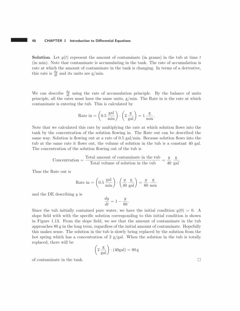
46 CHAPTER 1 Introduction to Differential Equations
Solution. Let y(t) represent the amount of contaminate (in grams) in the tub at time t(in min). Note that contaminate is accumulating in the tank. The rate of accumulation israte at which the amount of contaminate in the tank is changing. In terms of a derivative,this rate is dy
dt and its units are g/min.
We can describe dydt using the rate of accumulation principle. By the balance of units
principle, all the rates must have the same units, g/min. The Rate in is the rate at whichcontaminate is entering the tub. This is calculated by
Rate in =
(
0.5gal
min
)
·(
2g
gal
)
= 1g
min.
Note that we calculated this rate by multiplying the rate at which solution flows into thetank by the concentration of the solution flowing in. The Rate out can be described thesame way. Solution is flowing out at a rate of 0.5 gal/min. Because solution flows into thetub at the same rate it flows out, the volume of solution in the tub is a constant 40 gal.The concentration of the solution flowing out of the tub is
Concentration =Total amount of contaminate in the tub
Total volume of solution in the tub=
y
40
g
gal.
Thus the Rate out is
Rate in =
(
0.5gal
min
)
·(
y
40
g
gal
)
=y
80
g
min
and the DE describing y isdy
dt= 1− y
80.
Since the tub initially contained pure water, we have the initial condition y(0) = 0. Aslope field with with the specific solution corresponding to this initial condition is shownin Figure 1.13. From the slope field, we see that the amount of contaminate in the tubapproaches 80 g in the long term, regardless of the initial amount of contaminate. Hopefullythis makes sense. The solution in the tub is slowly being replaced by the solution from thehot spring which has a concentration of 2 g/gal. When the solution in the tub is totallyreplaced, there will be
(
2g
gal
)
· (40gal) = 80 g
of contaminate in the tank.
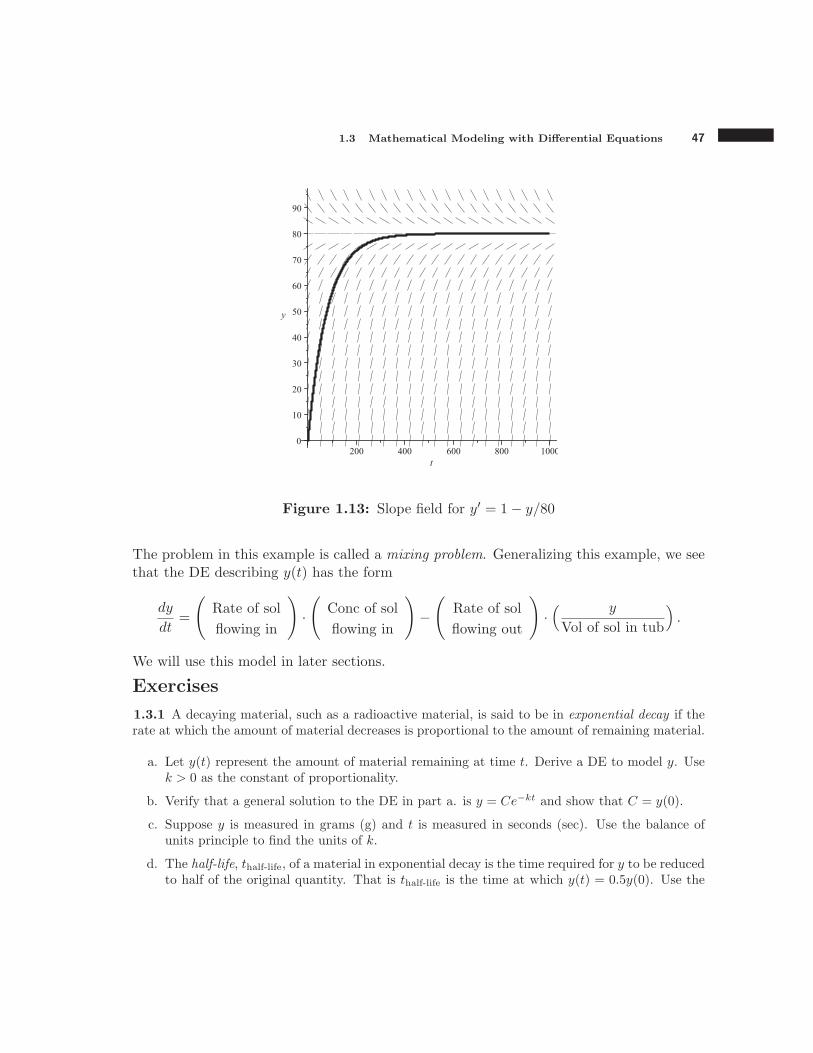
1.3 Mathematical Modeling with Differential Equations 47
Figure 1.13: Slope field for y′ = 1− y/80
The problem in this example is called a mixing problem. Generalizing this example, we seethat the DE describing y(t) has the form
dy
dt=
(
Rate of sol
flowing in
)
·(
Conc of sol
flowing in
)
−(
Rate of sol
flowing out
)
·( y
Vol of sol in tub
)
.
We will use this model in later sections.
Exercises
1.3.1 A decaying material, such as a radioactive material, is said to be in exponential decay if therate at which the amount of material decreases is proportional to the amount of remaining material.
a. Let y(t) represent the amount of material remaining at time t. Derive a DE to model y. Usek > 0 as the constant of proportionality.
b. Verify that a general solution to the DE in part a. is y = Ce−kt and show that C = y(0).
c. Suppose y is measured in grams (g) and t is measured in seconds (sec). Use the balance ofunits principle to find the units of k.
d. The half-life, thalf-life, of a material in exponential decay is the time required for y to be reducedto half of the original quantity. That is thalf-life is the time at which y(t) = 0.5y(0). Use the
48 CHAPTER 1 Introduction to Differential Equations
general solution in part b. to show that
thalf-life = −1
kln
(
1
2
)
≈ 0.69315
k.
e. The radioactive isotope plutonium-239 has a half-life of about 24, 000 years. If initially thereis 1 g of plutonium-239, approximate the time at which there is 0.8 g remaining.
1.3.2 Use the model mv′ = −cv |v| −mg for an object falling through a fluid medium (assumingturbulent flow) to estimate the time it will take a dropped crumpled piece of paper (initially zerovelocity) to reach a velocity of 2meter
sec in the downward direction. Assume that m is 0.0045 kilogramsand that c = 0.009 newtons·sec2/meter2. Thus c
m = 2 so that the differential equation becomesv′ = 2v2 − 9.8. We have divided the differential equation by m and replaced v |v| with −v2 becausev is negative for a falling object. Use whatever method(s) you think are most appropriate for thisproblem (algebraic, numerical or graphical). Will the paper ever reach a velocity of 3meter
sec in thedownward direction? Explain.
1.3.3 For the model mv′ = −cv|v|p−1 − mg of an object falling through a fluid medium, explainhow the parameter p affects the the graph of v versus t. For simplicity assume that m = c = 1 andg = 9.8. Also assume that v(0) = 0 to represent an object dropped from rest. Recall that p = 1represents laminar flow and p = 2 represents turbulent flow; consider values of p ranging between0.1 and 5. Use whatever method(s) you think are most appropriate. Give an interpretation of youranswer in terms of the falling object.
Note: when graphing the results of a numerical method, be sure to try different step sizes before youbelieve that the graph is accurate. A good rule of thumb for Euler’s method is to try two differentstep sizes with the second step size 1
10 of the first (such as 0.01 and 0.001); if the results are thesame to a given number of digits, then those digits are accurate. For graphs, the graphs for thetwo different step sizes should appear to be (almost) the same. The theory behind this rule will bedeveloped in Chapter 2.
Chapter 2
First-order Differential Equations
In this chapter we delve deeper into the various types of solutions (explicit, numerical, andgraphical) to first-order DE’s. In particular, we begin to develop methods for finding explicitsolutions. These methods depend highly on the form of the DE; different forms requiredifferent methods. There is no “one size fits all” method for finding explicit solutions. Inthis text we discuss only a small number of the methods available to mathematicians forfinding explicit solutions. More advanced texts discuss many additional methods.
In the first part of this chapter we discuss linear first-order equations. The distinctionbetween linear and nonlinear differential equations is perhaps the most important thatwe will make throughout this entire text. In general, linear DE’s of all orders are muchbetter understood than nonlinear ones, are usually easier to solve, and have solutions whoseproperties are often much “nicer” than those of nonlinear equations. The analysis of first-order nonlinear equations is the focus of the rest of this chapter.
2.1 Linear first-order differential equations
In high school algebra, a linear function of a single variable x is a function of the form
f(x) = ax+ b
where a and b are constants. Any function that cannot be written in the form is callednonlinear. For instance, the functions
f(x) = x2 + 3, f(x) =1
x+ 3, and f(x) = cos(x)
49
50 CHAPTER 2 First-order Differential Equations
are all nonlinear. A linear differential equation is a DE that can be written in a certain form.Linear DE’s can be of any order. In this section we deal with only first-order equations.
Definition 2.1.1 A first-order differential equation is said to be linear if it can bewritten in the form
y′ + g(x)y = h(x)
where g(x) and h(x) are functions of the independent variable. This form is calledthe standard form of a first-order linear DE.
Several comments can help clarify this definition:
1. The variables y and x are generic names for the dependent and independent variables,respectively. Any letter can be used for the names of these variables.
2. Parameters can appear in the functions g(x) and h(x). Also, these functions can beconstant functions. For example, in the DE y′+y = 2 we have g(x) = 1 and h(x) = 2.
3. The functions g(x) and h(x) need not be linear functions of x.
4. A linear DE is often more easily identified by what it does not contain. A linear DEcannot contain the dependent variable, or any of its derivatives, raised to a power,in an exponent, in a denominator, or inside a trig function. Nor can the dependentvariable, or any of its derivatives, be multiplied by any of its derivatives.
To determine if a given DE is linear or not, we need to determine if we can algebraicallyrewrite the equation into standard form. If we can, then the DE is linear. If we can’t, thenit’s not linear.
Example 2.1.1 Determine whether each of the following DE’s is linear or not. If it is linear,identify the functions g and h.
a. y′ + 2y = 3x+ 2 b. y′ + 2y2 = ex c. y′ = 2y
d. y′ = cos(x)y +1
x2 + 1e. yy′ = x2 f. x′ + t2x = et
Solution.
a. This DE is already in standard form where g(x) is the constant function 2 and h(x) =3x+ 2.
2.1 Linear first-order differential equations 51
b. This DE is not linear because of the y2 term.
c. We can rewrite this DE as y′ − 2y = 0, so it is linear with g(x) = −2 and h(x) = 0.
d. We can rewrite this DE as y′−cos(x)y = 1/(
x2 + 1)
, so it is linear with g(x) = cos(x)and h(x) = 1/
(
x2 + 1)
. Notice that g and h are not linear functions of x. However,this is not important.
e. This DE contains the product of y and y′. Thus it is not linear. We might be temptedto try to rewrite it into the standard form, but we will be unsuccessful.
f. In this differential equation, the dependent variable is x and the independent variableis t. Note that the coefficient of the dependent variable is a function of the independentvariable and that the right-hand side of the DE is a function of the independentvariable. Thus this DE is linear with g(t) = t2 and h(t) = et.
One reason that first-order DE’s are nice to work with is that there is a standard method offinding explicit solutions. To motivate this method, recall the product rule for derivativesfrom calculus:
d
dx(f(x)g(x)) = f ′g + fg′.
Example 2.1.2 To illustrate how the product rule can be used to find an explicit solution,consider the DE xy′+ y = 1. This equation could be rewritten into the form of a linear DE(the reader should verify this), but this is not necessary. Observe that by the product rule,
d
dx(xy) = 1y + xy′ = xy′ + y
so that the DE can be written asd
dx(xy) = 1.
Integrating both sides with respect to x gives
∫
d
dx(xy) dx =
∫
1 dx ⇒ xy = x+ C
where C is an arbitrary constant. Solving for y yields
y = 1 +C
x
which is a general solution.
52 CHAPTER 2 First-order Differential Equations
Not all linear DE’s are as simple as the previous example. To solve more complicatedexamples, recall the general exponential rule from calculus:
d
dxef(x) = eff ′
where f(x) is a function of x. Combining the product and exponential rules, we get thefollowing formula:
d
dx
(
yef(x))
= y′ef + yeff ′ (2.1)
where y is a function of x. The next example illustrates how this formula can be used tosolve linear DE’s.
Example 2.1.3 Consider the linear first-order DE y′ + 2y = 3. Observe that the left-handside of this DE resembles the right-hand side of equation (2.1), but without the exponentialterms. To make these look more similar, we calculate the following quantity:
µ(x) = e∫2 dx = e2x.
Then we multiply both sides of the DE by µ = e2x:
e2x(
y′ + 2y)
= 3e2x ⇒ y′e2x + 2ye2x = 3e2x.
Next comes the key step. Comparing the left-hand side of this equivalent version of the DEto the right-hand side of equation (2.1), we see that the DE is equivalent to
d
dx
(
ye2x)
= 3e2x.
Integrating both sides with respect to x yields
∫
d
dx
(
ye2x)
dx =
∫
3e2xdx ⇒ ye2x =3
2e2x + C
where C is an arbitrary constant. Solving for y yields
y =3
2+ Ce−2x.
This is a general solution to the DE.
The function µ(x) calculated in this example is called an integrating factor. We generalizethis example in the integrating factor method for solving first-order linear DE’s
2.1 Linear first-order differential equations 53
The Integrating Factor Method
Purpose: To find an explicit solution to a first-order linear DE.
1. Put the equation in the standard form y′+ g(x)y = h(x), if it is not already.
2. Calculate the integrating factor
µ(x) = e∫g(x) dx.
3. Multiply both sides of the DE by µ(x). The result can be rewritten in theform
d
dx[yµ(x)] = h(x)µ(x).
4. Integrate both sides of the DE in step 3 with respect to x to get
yµ(x) =
∫
h(x)µ(x) dx+ C.
5. Solve the equation in step 4 for y to get
y = µ−1
∫
hµdx+ Cµ−1.
In step 2,∫
g(x) dx represents any antiderivative of g(x), even though we leave off +Cfor simplicity. Also, in step 5, µ−1 mean 1/µ, not the inverse function of µ. Finally, wecould simply memorize the final formula in step 5. However, we don’t recommend this. Werecommend going through the steps each time, as they are not difficult and they help usremember why the method works.
Example 2.1.4 Use the integrating factor method to solve the DE y′ + y cos(t) = cos(t).
Solution. We follow the 5 steps outlined above:
Step 1: This DE is already in standard form with t as the independent variable andg(t) = cos(t).
54 CHAPTER 2 First-order Differential Equations
Step 2: µ = e∫cos(t) dt = esin(t)
Step 3: y′esin(t) + y cos(t) esin(t) = cos(t) esin(t) ⇒ d
dt
(
yesin(t))
= cos(t) esin(t)
Step 4:∫ d
dt
(
yesin(t))
dt =∫
cos(t) esin(t)dt ⇒ yesin(t) = esin(t) + C
Step 5: y = e− sin(t)esin(t) + Ce− sin(t) = 1 + Ce− sin(t)
Therefore, a general solution is y = 1 + Ce− sin(t).
In the previous example, the integrating factor method was relatively easy to apply. How-ever, in other cases the integrals
∫
g(x) dx or∫
h(x)µ(x) dx cannot be calculated in termsof elementary functions. In these cases the method fails to give an explicit solution. Thenext example illustrates one such case.
Example 2.1.5 Try to use the integrating factor method to solve the DE y′ + y =√x.
Solution. We try to follow the 5 steps:
Step 1: This DE is already in standard form with x as the independent variable andg(x) = 1.
Step 2: µ = e∫1 dx = ex
Step 3: y′ex + yex =√xex ⇒ d
dx(yex) =
√xex
Step 4:∫ d
dx(yex) dx =
∫ √xexdx ⇒ yex =
∫ √xexdx
The integral on the right in step 4 cannot be evaluated in terms of elementary functions(some computer algebra systems return a result in terms of the special function erf, some interms of the special function erfi, and some simply return the integral itself indicating thatan antiderivative cannot not be found). Thus the method fails to give an explicit solution.We could write the solution as y = e−x
∫ √xexdx+Ce−x but this is not an explicit solution
in terms of elementary functions.
Applications
The integrating factor method can be used to find the explicit solutions of real-world prob-lems as illustrated in the next two examples.
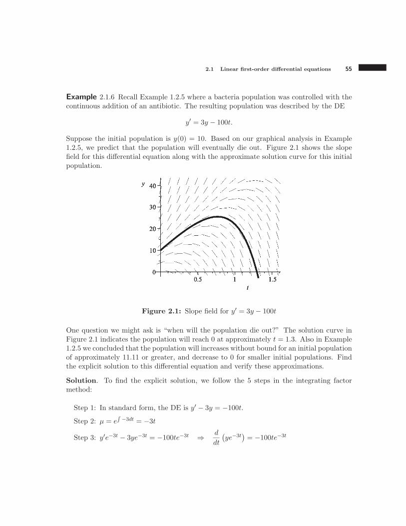
2.1 Linear first-order differential equations 55
Example 2.1.6 Recall Example 1.2.5 where a bacteria population was controlled with thecontinuous addition of an antibiotic. The resulting population was described by the DE
y′ = 3y − 100t.
Suppose the initial population is y(0) = 10. Based on our graphical analysis in Example1.2.5, we predict that the population will eventually die out. Figure 2.1 shows the slopefield for this differential equation along with the approximate solution curve for this initialpopulation.
Figure 2.1: Slope field for y′ = 3y − 100t
One question we might ask is “when will the population die out?” The solution curve inFigure 2.1 indicates the population will reach 0 at approximately t = 1.3. Also in Example1.2.5 we concluded that the population will increases without bound for an initial populationof approximately 11.11 or greater, and decrease to 0 for smaller initial populations. Findthe explicit solution to this differential equation and verify these approximations.
Solution. To find the explicit solution, we follow the 5 steps in the integrating factormethod:
Step 1: In standard form, the DE is y′ − 3y = −100t.
Step 2: µ = e∫−3dt = −3t
Step 3: y′e−3t − 3ye−3t = −100te−3t ⇒ d
dt
(
ye−3t)
= −100te−3t
56 CHAPTER 2 First-order Differential Equations
Step 4:∫ d
dt
(
ye−3t)
dt =∫
−100te−3tdt ⇒ ye−3t =100
9e−3t +
100
3te−3t + C (the
integral on the right is evaluated using integration by parts or with software)
Step 5: y =100
9+
100
3t+ Ce3t
If y(0) = 10, then
10 =100
9+
100
3(0) + Ce3(0) = C +
100
9⇒ C = −10
9
so that the particular solution is
y =100
9+
100
3t− 10
9e3t.
To find the exact time at which the population dies out, we set y equal to 0 and solve for t.The resulting equation cannot be solved algebraically, but it can be solved numerically usingsoftware. Software gives the solutions t = 1.29657 and t = −0.32059. The negative valueof t makes no sense, so we ignore this solution. This confirms our graphical approximationof t.
To analyze how the initial condition affects the long-term behavior of the solution, weexamine the general solution found in Step 5. Note that there is a linear part, 100/9 +(100/3)t, which is positive for all t > 0. There is also an exponential part, Ce3t whose signdepends on the sign of C. Thus the long-term behavior of the solution depends on the signof C. We analyze these three cases separately:
1. If C = 0, then the solution is y = 100/9 + (100/3)t, whose graph is a straight line.The initial population would be y(0) = 100/9 ≈ 11.11.
2. If C > 0, then y(t) > y(0) for all t. Thus the population would be continuallyincreasing.
3. If C < 0, then “eventually” the negative exponential part Ce3t would dominate thepositive linear part causing y(t) to become negative, meaning the population dies out.
This algebraic analysis confirms our graphical analysis. Figure 2.2 illustrates these threecases.
Admittedly, in this situation the additional accuracy gained by the algebraic analysis maynot be terribly useful. The point here is that an algebraic analysis of a general solutiongives higher levels of accuracy than other methods.

2.1 Linear first-order differential equations 57
Figure 2.2: Slope field and solution curves for y′ = 3y − 100t
Example 2.1.7 In section 1.3 we derived Newton’s law of cooling,
dT
dt= k(A− T )
where A is the constant room temperature, k is a constant, T is the temperature of theobject, and t is time.
Suppose that a pizza stone is removed from an oven at 375◦F and set on a table in a roomat 70◦F. After 1/4 of an hour, the temperature of the stone is 150◦F. Using Newton’s lawof cooling, find the exact time at which the stone reaches 90◦F.
Solution. First we find a general solution to Newton’s law of cooling using the integratingfactor method. Rather than substituting A = 70 into the differential equation at thebeginning, we choose to leave A as a parameter and get the general solution in terms of A.This gives us a result that we can reuse in other situations.
Step 1: T ′ + kT = kA.
Step 2: µ = e∫k dt = ekt
Step 3: T ′ekt + kTekt = kAekt ⇒ d
dt
(
Tekt)
= kAekt
Step 4:∫ d
dt
(
Tekt)
dt =∫
kAektdt ⇒ Tekt = Aekt + C
58 CHAPTER 2 First-order Differential Equations
Step 5: T = A+ Ce−kt
We now substitute in A = 70 to obtain the general solution T = 70+Ce−kt. We still mustdetermine the integration constant C and proportionality constant k. To determine k, wesummarize the information given in the problem in the form of a table:
t 0 0.25 ?
T 375 150 90
The first data point gives
375 = 70 + Ce−k(0) ⇒ C = 305.
Using this value of C and the second data point we get
150 = 70 + 305e−k(0.25) ⇒ k = − 1
0.25ln(
80
305) ≈ 5.3531.
This yields the specific solution T = 70 + 305e−5.3531t.
To find the time at which the stone reaches 90◦F, we set T = 90 and solve for t:
90 = 70 + 305e−5.3531t ⇒ t = − 1
5.3531ln(
20
305) ≈ 0.50897.
Thus the pizza stone will reach 90◦F in about 0.51 hours.
Example 2.1.8 Consider a tank that contains 50 gal of a solution composed of 90% waterand 10% alcohol. A second solution containing 50% alcohol is added to the tank at therate of 2 gal/min. At the same time, solution is being drained from the tank at the rateof 3 gal/min. Assuming the tank is continuously stirred, describe the volume of alcohol inthe tank, and the concentration of alcohol, at any time.
Solution. Let y (t) represent the volume (in gal) of alcohol in the tank at time t (in min).In Section 1.3 we derived the following general model for y:
dy
dt=
(
Rate of sol
flowing in
)
·(
Conc of sol
flowing in
)
−(
Rate of sol
flowing out
)
·( y
Vol of sol in tank
)
.
Since the rate of solution flowing in is different than the rate flowing out, the volumeof solution in the tank is not constant. To describe this volume, we can use the rate of
2.1 Linear first-order differential equations 59
accumulation principle:
Change in vol of sol in tank = 2gal
min− 3
gal
min= −1
gal
min.
This means that the overal volume of solution in the tank is decreasing by 1 gal/min sothat the volume of solution in the tank at time t is (50 − t) gal. Therefore, the model fory is
dy
dt= 2(0.5)− 3
(
y
50− t
)
= 1− 3y
50− t.
We are told that initially the solution in the tank is 90% alcohol. Since the tank originallycontained 50 gal, the initial amount of alcohol in the tank is 50(0.9) = 45. This means wehave the initial condition y(0) = 45. This is a linear first-order IVP which we can solveusing the integrating factor method.
Step 1: In standard form, the DE is y′ +3
50− ty = 1.
Step 2: µ = e∫3/(50−t)dt = e−3 ln(50−t) = (50− t)−3
Step 3: y′(50− t)−3+ 350−t y(50− t)−3 = 1(50− t)−3 ⇒ d
dt
(
y(50− t)−3)
= (50− t)−3
Step 4:∫ d
dt
(
y(50− t)−3)
dt =∫
(50− t)−3dt ⇒ y(50− t)−3 = 12(50− t)−2 + C
Step 5: y = 12(50− t) + C(50− t)3
The initial condition y(0) = 45 yields
45 = y(0) =1
2(50− 0) + C(50− 0)3 = 25 + 503C ⇒ C = 0.00016
which gives the specific solution
y(t) = 0.00016(50− t)3 − 1
2t+ 25 = 0.00016(50− t)3 +
50− t
2.
This function describes the volume of alcohol in the tank at any point in time. Note thatthe tank is completely drained at time t = 50 so this function is defined only for 0 ≤ t ≤ 50.The concentration of the solution in the tank at time t, c(t), is then
c(t) =y
Vol of sol in tank=
y
50− t= 0.00016(50− t)2 +
1
2.
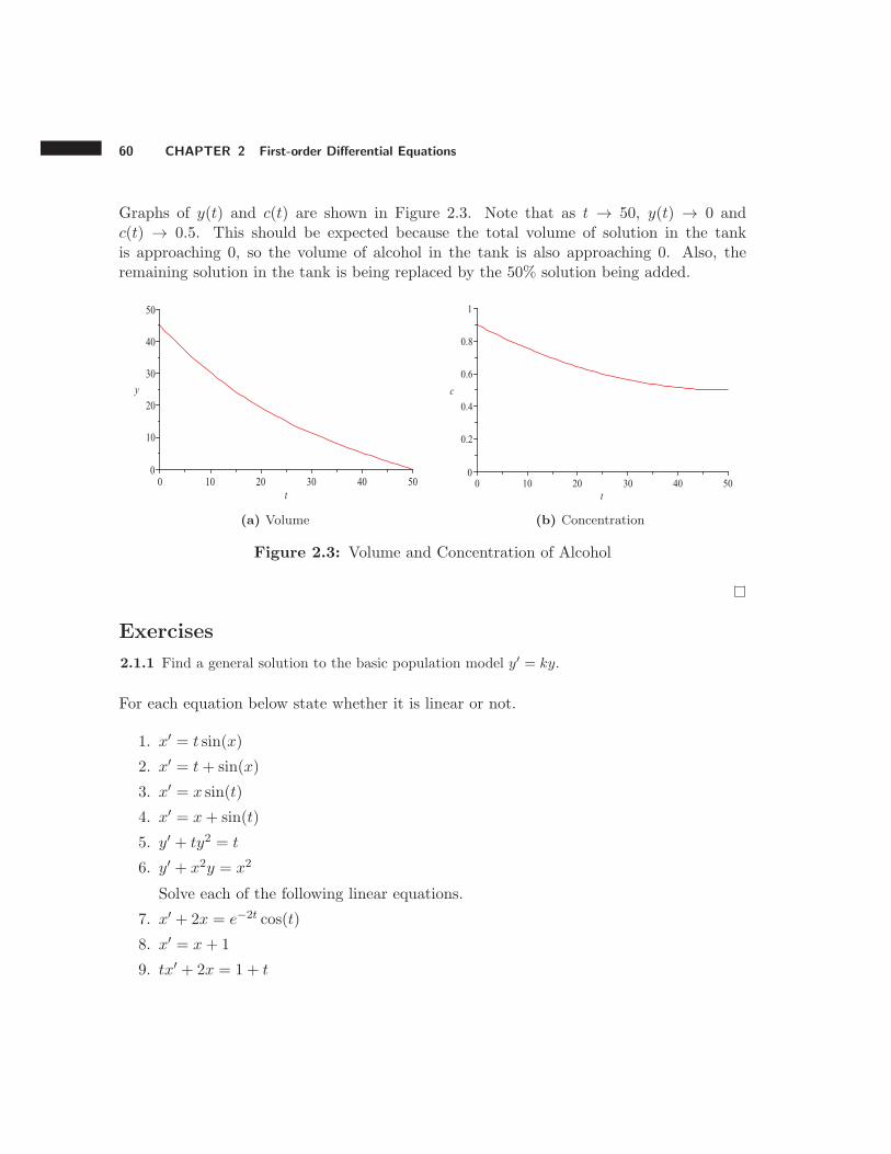
60 CHAPTER 2 First-order Differential Equations
Graphs of y(t) and c(t) are shown in Figure 2.3. Note that as t → 50, y(t) → 0 andc(t) → 0.5. This should be expected because the total volume of solution in the tankis approaching 0, so the volume of alcohol in the tank is also approaching 0. Also, theremaining solution in the tank is being replaced by the 50% solution being added.
(a) Volume (b) Concentration
Figure 2.3: Volume and Concentration of Alcohol
Exercises
2.1.1 Find a general solution to the basic population model y′ = ky.
For each equation below state whether it is linear or not.
1. x′ = t sin(x)
2. x′ = t+ sin(x)
3. x′ = x sin(t)
4. x′ = x+ sin(t)
5. y′ + ty2 = t
6. y′ + x2y = x2
Solve each of the following linear equations.
7. x′ + 2x = e−2t cos(t)
8. x′ = x+ 1
9. tx′ + 2x = 1 + t
2.2 Existence, uniqueness, and portraits for first-order equations 61
10. x′ = x+ t
Solve the following initial-value problems:
11. x′ = x+ e3t, x(0) = 2
12. x′ + 2x = e−2t cos(t), x(0) = 1
13. tx′ + x = t2 + t, x(1) = 0
14. x′ + 2tx = t, x(0) = 1
2.2 Existence, uniqueness, and portraits for first-order equa-
tions
Up to now, we have talked about how to describe the solution(s) to a differential equation indifferent ways: explicit, numerical, and graphical. In this section we discuss three somewhatmore theoretical questions about IVP’s:
1. When do we know that a solution to an initial value problem exists?
2. If a solution does exist, is it the only one?
3. If a solution does exist, on what interval of the independent variable is it valid?
When we talk about existence in this section, we do not mean existence of an explicitsolution in terms of elementary functions. Any function will do, whether given in terms ofinfinite series, integrals, or other limiting processes. In other words, any way of generatinga value of the dependent variable for a given value of the independent variable is acceptableas long as the resulting function “works” as a solution to the differential equation.
We start with a theorem that answers all three of these questions for linear first-order IVP’s.In the proof we derive a formula for the specific solution to such an IVP. This formula isbased on the formula for a general solution to a first-order DE y′ + g(x)y = h(x) found instep 5 of the integrating factor method,
y = µ−1
∫
hµ dx+ Cµ−1
where µ = e∫g(x) dx.
62 CHAPTER 2 First-order Differential Equations
Theorem 2.1 (Existence/Uniqueness for Linear First-Order IVP’s) Consider an IVP ofthe form
y′ + g(x) y = h(x), y (x0) = y0.
Assume that g(x) and h(x) are both continuous on some interval a < x < b and thata < x0 < b. Then there exists a unique solution y(x) to the IVP that is defined ona < x < b.
Proof. To prove existence, consider the function
y(x) =1
µ(x)
∫ x
x0
h(s)µ(s) ds+ y01
µ(x)
where µ(x) = e∫x
x0g(s)ds
. We will show that y(x) is a solution to the IVP. First note that
µ (x0) = e∫x0x0
g(s)ds= e0 = 1.
Thus
y (x0) =1
µ (x0)
∫ x0
x0
h(s)µ(s) ds+ y01
µ (x0)=
1
1· 0 + y0 ·
1
1= y0
showing that this function satisfies the initial condition. To show that this function satisfiesthe DE, note that by the Fundamental Theorem of Calculus,
d
dxµ(x) = e
∫x
x0g(s)ds · d
dx
∫ x
x0
g(s)ds = µ(x)g(x).
For notational simplicity, let a(x) =∫ xx0
h(s)µ(s) ds so that y(x) = 1µ · a + y0
1µ (we have
further simplied notation by dropping the x). Then ddx a(x) = h(x)µ(x) and
d
dxy(x) = − 1
µ2· µ′ · a+
1
µ· a′ − y0
1
µ2· µ′
= − 1
µ2· µ · g · a+
1
µ· h · µ− y0
1
µ2· µ · g
= − 1
µ· g · a+ h− y0
1
µ· g.
Then
y′ + g · y = − 1
µ· g · a+ h− y0
1
µ· g + g · 1
µ· a+ g · y0
1
µ= h
Thus y(x) solves the DE which proves that a solution to the IVP does exist. Note that we
2.2 Existence, uniqueness, and portraits for first-order equations 63
may not be able to evaluate this formula for y(x) in terms of elementary functions, but thiswas never claimed in the theorem.
Note also that this solution is defined on a < x < b, because the integrals
∫ x
x0
g(s) ds and
∫ x
x0
h(s)µ(s) ds
which appear in the formula for y(x) both exist on a < x < b due to the continuity of g(x)and h(x) on the interval a < x < b.
To prove uniqueness, suppose that y1(x) and y2(x) both satisfy the IVP. Define z(x) =y1(x)− y2(x). Then
z′ + g · z = y′1 − y′2 + g · y1 − g · y2 = (y′1 + g · y1) + (y′2 + g · y2)
Since both y1 and y2 satisfy the DE,
(y′1 + g · y1) + (y′2 + g · y2) = h− h = 0
and hencez′ + g · z = 0.
Solving this DE with the integrating factor method, we get z = Ce−∫g dx and that
z(x0) = y1(x0)− y2(x0) = y0 − y0 = 0.
But the only way that an exponential function such as Ce−∫g dx can equal 0 for even one
value of x is if C = 0. This means that z(x) = 0 for all x and hence
y1(x) = y2(x)
for all x, verifying uniqueness.
A solution to an IVP as described in Theorem 2.1 is a function. It may appear that thisfunction could be evaluated at many different values of x. But the theorem states that thesolution only exists on an interval on which g(x) and h(x) are both continuous and x0 mustbelong to this interval. The next example illustrates this point.
Example 2.2.1 Solve the initial value problem xy′ + y = 10, y(1) = 1, and determine thelargest interval of existence.
Solution. We use the integrating factor method to find a general solution:
64 CHAPTER 2 First-order Differential Equations
Step 1: y′ +y
x=
10
x
Step 2: µ = e
∫ 1
xdx
= elnx = x
Step 3: xy′ + x · yx= x · 10
x⇒ d
dx(xy) = 10
Step 4:∫
d (xy) =∫
10 dx ⇒ xy = 10 + C
Step 5: y = 10 + Cx
Using y(1) = 1 we get 1 = 10 + C so C = −9. Thus the particular solution to the IVP isy = 10− 9
x .
Note that this solution is a function. It appears that we could evaluate this function atany x 6= 0. However, we have g(x) = 1
x and h(x) = 10x which are both continuous on the
intervals x < 0 and x > 0. Since x0 = 1 is part of the interval x > 0, the largest intervalof existence is also x > 0. This means that the solution y = 10 − 9
x is defined only forx > 0.
Theorem 2.1 applies to first-order IVP’s of a certain form. We now state an existenceand uniqueness theorem for any first-order IVP. This theorem applies to both linear andnonlinear problems.
Theorem 2.2 (Existence/Uniqueness for General First-Order IVP’s) Consider a first-orderIVP of the form
y′ = f(x, y), y (x0) = y0.
Assume that f(x, y) and ∂∂yf(x, y) are both continuous on a region in the xy-plane given
by a < x < b and c < y < d, and that this region contains the point (x0, y0). Then thereexists a unique solution y(x) to the IVP, defined on some interval α < x < β which iscontained in the interval a < x < b.
Proof. The proof of this theorem is beyond the scope of this text. The reader is referred tothe classic text Theory of Ordinary Differential Equations by Earl Coddington and NormanLevinson (1955), or to the website http://en.wikipedia.org/wiki/Picard-Lindelof_
theorem.
Note that with this theorem, the region a < x < b, c < y < d where the premises of thetheorem are satisfied can be large, and yet the interval α < x < β can be quite small. Oneimportant difference between Theorems 2.1 and 2.2 is that for linear differential equations,
2.2 Existence, uniqueness, and portraits for first-order equations 65
the largest interval of existence can be determined before the solution is found, whereasfor nonlinear equations, generally one must first find the solution and then determine theinterval of existence from that.
In the next section we present a method for solving certain types of nonlinear DE’s (onesthat are called separable). For the next example, we resort to computer algebra to determinea solution to a nonlinear equation, and then from it we state the interval of existence.
Example 2.2.2 Use available software to find a solution to the IVP y′ = y2, y(0) = 5, andthen determine the largest interval on which that solution is defined. Is your solution theonly one for which y(0) = 5?
Solution. First note that f(x, y) = y2 and ∂F∂y = 2y, both of which are continuous
everywhere in the xy-plane. This region certainly contains the point (0, 5). Thus Theorem2.2 applies to this IVP.
The solution given by Wolfram Alpha is
y =5
1− 5x.
We could evaluate this function for x < 15 and x > 1
5 . However, since x0 = 0 < 15 , we
conclude that as a solution to the IVP, this function is defined for only x < 15 . Theorem
2.2 guarantees that this solution is unique.
One thing to take away from the previous example is that solutions to differential equationscan’t “jump over” asymptotes. The function y = 5
1−5x has a vertical asumptote at x = 15 .
However, the solution to the IVP is only defined for x < 15 . This means that we must be
careful when using explicit solutions to nonlinear differential equations. Suppose that wewanted to know the value of y(1). It is tempting, but quite wrong, to just substitute x = 1into the explicit solution y = 5
1−5x to get y = −54 . The absurdity of this answer becomes
obvious when we look at a slope field in Figure 2.4.
The slope fields shows that all solution curves must be increasing from left to right, sinceall slope marks have positive or zero slopes. Therefore, the solution curve depicted cannotgo through the point (1, −5/4) because the curve would have to decrease.
In previouse examples we have seen solutions to IVP’s y(x) such that limx→∞ y(x) = ∞.Note that in Example 2.2.2, we have limx→1/5− y(x) = ∞. The fact that this limit is infinitefor x approaching a finite number is referred to as finite time blow-up. In such a case, itmakes no sense to talk about the long-term behavior (as x → ∞) of the solution, since thesolution “ends” at a finite value of the independent variable. Finite time blow-up can occurfor either linear or nonlinear DE’s.
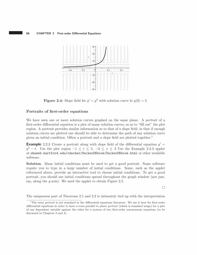
66 CHAPTER 2 First-order Differential Equations
Figure 2.4: Slope field for y′ = y2 with solution curve fo y(0) = 5.
Portraits of first-order equations
We have seen one or more solution curves graphed on the same plane. A portrait of afirst-order differential equation is a plot of many solution curves, so as to “fill out” the plotregion. A portrait provides similar information as to that of a slope field, in that if enoughsolution curves are plotted one should be able to determine the path of any solution curvegiven an initial condition. Often a portrait and a slope field are plotted together.1
Example 2.2.3 Create a portrait along with slope field of the differential equation y′ =y2 − t. Use the plot region −1 ≤ t ≤ 5, −3 ≤ x ≤ 3 Use the Example 2.2.3 appletat uhaweb.hartford.edu/rdecker/DeckerDEbook/DeckerDEbook.html or other availablesoftware.
Solution. Many initial conditions must be used to get a good portrait. Some softwarerequire you to type in a large number of initial conditions. Some, such as the appletreferenced above, provide an interactive tool to choose initial conditions. To get a goodportrait, you should use initial conditions spread throughout the graph window (not just,say, along the y-axis). We used the applet to obtain Figure 2.5.
The uniqueness part of Theorems 2.1 and 2.2 is intimately tied up with the interpretation
1The term portrait is not standard in the differential equations literature. We use it here for first-orderdifferential equations in order to have a term parallel to phase portrait (which is standard usage) for a plotof one dependent variable against the other for a system of two first-order autonomous equations (to bediscussed in Chapters 3 and 4).
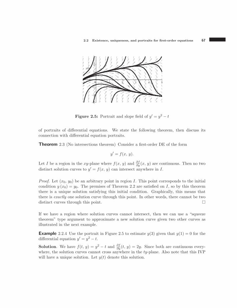
2.2 Existence, uniqueness, and portraits for first-order equations 67
Figure 2.5: Portrait and slope field of y′ = y2 − t
of portraits of differential equations. We state the following theorem, then discuss itsconnection with differential equation portraits.
Theorem 2.3 (No intersections theorem) Consider a first-order DE of the form
y′ = f(x, y).
Let I be a region in the xy-plane where f(x, y) and ∂f∂y (x, y) are continuous. Then no two
distinct solution curves to y′ = f(x, y) can intersect anywhere in I.
Proof. Let (x0, y0) be an arbitrary point in region I. This point corresponds to the initialcondition y (x0) = y0. The premises of Theorem 2.2 are satisfied on I, so by this theoremthere is a unique solution satisfying this initial condition. Graphically, this means thatthere is exactly one solution curve through this point. In other words, there cannot be twodistinct curves through this point.
If we have a region where solution curves cannot intersect, then we can use a “squeezetheorem” type argument to approximate a new solution curve given two other curves asillustrated in the next example.
Example 2.2.4 Use the portrait in Figure 2.5 to estimate y(3) given that y(1) = 0 for thedifferential equation y′ = y2 − t.
Solution. We have f(t, y) = y2 − t and ∂f∂y (t, y) = 2y. Since both are continuous every-
where, the solution curves cannot cross anywhere in the ty-plane. Also note that this IVPwill have a unique solution. Let y(t) denote this solution.
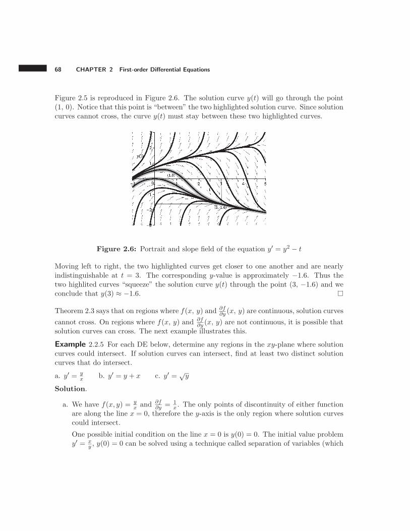
68 CHAPTER 2 First-order Differential Equations
Figure 2.5 is reproduced in Figure 2.6. The solution curve y(t) will go through the point(1, 0). Notice that this point is “between” the two highlighted solution curve. Since solutioncurves cannot cross, the curve y(t) must stay between these two highlighted curves.
Figure 2.6: Portrait and slope field of the equation y′ = y2 − t
Moving left to right, the two highlighted curves get closer to one another and are nearlyindistinguishable at t = 3. The corresponding y-value is approximately −1.6. Thus thetwo highlited curves “squeeze” the solution curve y(t) through the point (3, −1.6) and weconclude that y(3) ≈ −1.6.
Theorem 2.3 says that on regions where f(x, y) and ∂f∂y (x, y) are continuous, solution curves
cannot cross. On regions where f(x, y) and ∂f∂y (x, y) are not continuous, it is possible that
solution curves can cross. The next example illustrates this.
Example 2.2.5 For each DE below, determine any regions in the xy-plane where solutioncurves could intersect. If solution curves can intersect, find at least two distinct solutioncurves that do intersect.
a. y′ = yx b. y′ = y + x c. y′ =
√y
Solution.
a. We have f(x, y) = yx and ∂f
∂y = 1x . The only points of discontinuity of either function
are along the line x = 0, therefore the y-axis is the only region where solution curvescould intersect.
One possible initial condition on the line x = 0 is y(0) = 0. The initial value problemy′ = x
y , y(0) = 0 can be solved using a technique called separation of variables (which
2.2 Existence, uniqueness, and portraits for first-order equations 69
we cover in the next section), or we can use software. The general solution is y = Cx.Since the general solution satisfies y(0) = 0 for any value of C, there are infinitelymany solutions to the IVP, all of which intersect at the point (0, 0).
b. We have f(x, y) = y + x and ∂f∂x (x, y) = 1. These functions are both continuous for
all x and y, therefore solution curves cannot intersect anywhere.
c. We have f(x, y) =√y = y1/2 so that ∂f
∂y (x, y) = 12√y . Note that f(x, y) is defined
and continuous for y ≥ 0 and ∂f∂y (x, y) is discontinuous (and undefined) along y = 0.
Therefore solution curves could intersect along y = 0.
If we choose the initial condition y(0) = 0, then the specific solution is y = x2/4 forx ≥ 0. Another solution to the same initial value problem is y(x) = 0 for all x (seeExercise 2.2.2 for a verification of these solutions). These two solutions intersect atthe point (0, 0).
The last example illustrates that we must be very careful in using the predictions of anymathematical model, especially a DE which may not have a unique solution.
Example 2.2.6 (The miraculous population model) Consider the basic population modely′ = ky. If the initial condition is y(0) = 0, then a solution is y(t) = 0 for all t. By Theorem2.1, this solution is unique. This should should make intuitive sense. If we start with zeropopulation, we should always have zero population.
What if the population model were y′ = k√y? This DE models the assumption that
the rate of growth of the population is proportional to the square root of the size of thepopulation. Note that as y increases,
√y also increases, which means that y′ would also
increase. This does not seem too unreasonable. If k = 1 and we have the initial conditiony(0) = 0, we get two possible solutions for t ≥ 0:
y(t) =t2
4and y(t) = 0.
The solution y(t) = 0 makes perfect sense. However, the solution y(t) = t2/4 predicts thatthe population would increase for t > 0 even though we started with a population of 0. Itdoes not seem reasonable that this could actually happen (spontaneous generation of livingorganisms was once considered possible, but an experiment by Louis Pasteur in 1859 isconsidered to have ruled it out).
The solution y(t) = t2/4 is much more interesting than y(t) = 0. However, this exampleshows that the more interesting solution is not necessarily correct.
70 CHAPTER 2 First-order Differential Equations
Exercises
2.2.1 Use the integrating factor method to show that a general solution to the DE z′ + gz = 0 isz = Ce−
∫g dx.
2.2.2 Consider the IVPy′ =
√y, y(0) = 0.
a. Verify that y = 0 is a specific solution to this IVP.
b. Verify that y = x2/4 is a specific solution to this IVP.
c. Explain why the solution y = x2/4 is defined for only x ≥ 0. (Hint : Plug the solution into theDE. What is the sign of the right-hand side? What is the sign of the left-hand side if x < 0?)
2.2.3 Show that the differential equation x′ = x1+t2 has a unique solution through every initial
point (t0, x0). Can solution curves ever intersect for this differential equation?
2.2.4 Does the equation x′ = x2 − t have a unique solution through every initial point (t0, x0)?Can solution curves ever intersect for this differential equation? If so, where?
2.2.5 Does the equation x′ = x2/3 have a unique solution through every initial point (t0, x0)? Cansolution curves ever intersect for this differential equation? If so where? Can you find two solutioncurves that cross each other?
Use available software to create a detailed slope field and phase portrait for each equationbelow. Briefly describe the long-term behavior for various values of the initial conditionx(0).
2.2.6 x′ = x+ t/2.
2.2.7 x′ = x2(1− x)
2.2.8 x′ = 1 + t/2
2.2.9 dPdt = rP (1− P
N ) using the parameter values r = 0.5 and N = 10
2.3 Separable Differential Equations
Like a linear equation, a separable DE is an equation that can be written in a special formwhich leads to a solution method. We begin with a definition.
2.3 Separable Differential Equations 71
Definition 2.3.1 A first-order differential equation y′ = f(x, y) is said to be sepa-
rable if f(x, y) can be factored into the form
f(x, y) = g(x)h(y)
where g(x) is a function of only x and h(y) is a function of only y.
As with the integrating factor method for linear equations, the names of the dependentand independent variables are not important. For example if we wrote the DE as x′ =f(t, x), with t the independent variable and x the dependent variable, the requirement forseparability would be f(t, x) = g(t)h(x).
Example 2.3.1 Determine which of the following equations are separable.
a. y′ = xy b. x′ = xt+ x c. y′ = x+ y
d. y′ = 3et+y e. x′ = sin tcosx f. y′ = y
Solution.
a. Clearly separable with g(x) = x and h(y) = y.
b. Separable, since xt+ x can be factored into x(t+1). Then f(t) = t+1 and g(x) = x.
c. The right-hand side, x + y, cannot be factored into the form g(x)h(y) so this DE isnot separable. While we could factor as x(1 + y/x), this is no help as (1 + y
x) is not afunction of y alone.
d. Separable with 3et+y = 3etey so g(t) = 3et and h(y) = ey.
e. Separable sincesin t
cosx= sin t
(
1
cosx
)
.
f. Since the independent variable does not appear in the equation (such equations arecalled autonomous and will be studied in a later section) we can choose the name ofthe independent variable; let’s choose x. This equation is separable since y = 1 · y sothat g(x) = 1 and h(y) = y. Note that g(x) = 1 can be considered to be a constantfunction of x. Autonomous first-order equations are always separable.
72 CHAPTER 2 First-order Differential Equations
The next example helps motivate a relatively simple technique for finding an explicit solu-tion to a separable DE.
Example 2.3.2 Consider the separable DE y′ = xy. For simplicity we will add the restric-tion that y > 0. We can algebraically rewrite this DE as
y′
y= x. (2.2)
On the left-hand side of equation (2.2), we have the derivative of a function divided by thefunction. This should remind us of the general logarithmic rule from Calculus:
d
dxln [u(x)] =
u′
u
where u(x) > 0. So we can rewrite equation (2.2)
d
dxln y = x. (2.3)
Our goal is to get a formula for y. We are getting closer because we have gotten rid of y′.But now we have introduced a d
dx . To get ride of ddx , let’s try writing the right-hand side
of the DE in terms of a derivative with respect to x. Note that
d
dx
(
x2
2
)
= x. (2.4)
Thus we can rewrite equation (2.3) as
d
dxln y =
d
dx
(
x2
2
)
.
Now, ln y and x2/2 are functions whose derivatives are equal for all x. The only way thisis possible is if these two functions differ by a constant. Thus we have
ln y =x2
2+ C (2.5)
where C is an arbitrary constant. Now compare equations (2.2) and (2.5). Note that theleft-hand side of (2.5) is simply the antiderivative of the left-hand side of (2.2) where thevariable of integration is y. The right-hand sides share a similar relationship where the
2.3 Separable Differential Equations 73
variable of integration is x. In mathematical notation, we have shown that
∫
y′
ydy =
∫
x dx.
To finish the solution, we solve equation (2.5) for y:
eln y = ex2/2+C ⇒ y = ex
2/2+C .
This gives us an explicit general solution to the original DE.
We generalize this example in the method of separation of variables.
The Method of Separation of Variables
Purpose: To solve a DE of the form y′ = g(x)h(y).
Step 1: Replace y′ with dydx and rewrite the the DE in the form
1
h(y)dy = g(x)dx.
Step 2: Add an integral sign to both sides to get
∫
1
h(y)dy =
∫
g(x) dx
and then integrate both sides (if possible). Make sure to add a constantto the result on the right-hand side.
Step 3: Solve the equation that results from step 2 for the dependent variable (ifpossible).
Example 2.3.3 Use separation of variables to find the general solution to y′ = xy2.
Solution. We follow the three steps:
Step 1:dy
dx= xy2 ⇒ 1
y2dy = x dx
74 CHAPTER 2 First-order Differential Equations
Step 2:
∫
1
y2dy =
∫
x dx ⇒ 1
y=
1
2x2 + c where c is an arbitrary constant
Step 3: y =1
12x
2 + c
The expression for y in step 3 is OK, but we usually don’t like fractions within fractions.So we can do a little bit of algebra to the right-hand side to simplify things:
y =1
12x
2 + c· 22=
2
x2 + 2c.
To further simplify things, note that c is an arbitrary constant, so 2c is an arbitrary constant.Thus we define the arbitrary constant C = 2c and write the final solution as
y =2
x2 + C.
We always want to write the final solution in as simple terms as possible.
Example 2.3.4 Use separation of variables to find the general solution to y′ = y.
Solution. Note that the independent variable is not explicitly given. For somethingdifferent, we’ll use t.
Step 1:dy
dt= y ⇒ 1
ydy = 1 dt
Step 2:
∫
1
ydy =
∫
1 dt ⇒ ln |y| = t+ c
Step 3: eln |y| = et+c ⇒ |y| = et+c
Note that we put the absolute value signs around y in step 2 because we are not told thaty is always positive. As in the previous example, this description for y is OK, but we cansimplify it. Note that by properties of exponents we can write
|y| = et+c = etec.
But c is a constant, so ec is a constant. However, note that ec is positive. So define C tobe a positive constant. Then the solution can be written as
|y| = Cet.
2.3 Separable Differential Equations 75
To further simplify this solution, note that if y ≥ 0, then
|y| = y ⇒ y = Cet
and if y < 0, then|y| = −y ⇒ y = −Cet.
We can combine these two cases and allow for the possibility that y is positive or negativeby allowing C to be a positive or negative constant and writing the general solution as
y = Cet.
Changing the constant as we have done in the last two examples is sometimes referred toas “abusing the constant.”
Separation of variables can fail to yield an explicit solution if the integrals in step 2 cannotbe evaluated in terms of elementary functions, or we cannot solve for y in step 3. The nexttwo examples illustrate such cases.
Example 2.3.5 Attempt to use separation of variables to find the general solution to x′ =xext.
Solution. Note that the dependent variable is x and the independent variable is t.
Step 1:dx
dt= xext ⇒ 1
xexdx = t dt
Step 2:
∫
1
xexdx =
∫
t dt
The integral on the left cannot be expressed in terms of elementary functions. At the timeof the writing of this text, Wolfram Alpha gives Ei(−x), Maple returns −Ei(1, x), and the
TI89 returns∫
e−x
x dx (which means the TI89 cannot find the integral). When a specialfunction such as Ei(−x) or −Ei(1, x) appears in the result, one can consult the help filesfor the particular system used in order to find the definition of the special function. For ourpurposes, we can say that the method of separation of variables fails to give us an explicitsolution in terms of elementary functions.
Example 2.3.6 Use separation of variables to find the general solution to x′ =t
xex.
Solution. We follow the 3 steps:
Step 1:dx
dt=
t
xex⇒ xexdx = t dt
76 CHAPTER 2 First-order Differential Equations
Step 2:
∫
xexdx =
∫
t dt ⇒ xex − ex =1
2t2 + C. The integral on the left is
evaluated using integration by parts or software.
Step 3: We try to use software to solve for x. Wolfram Alpha runs out of time, Maplereturns RootOf(exp( Z) ∗ Z − Z − t − c), and the TI89 returns solve(2xex −2x− t2 − 2c = 0).
Since none of the software returns an explicit result for x in terms of t, we conclude thatno explicit solution for x in terms of elementary functions of t is possible. This is often thecase when the variable that we are solving for (x in this case) appears both in the argumentof an exponential function and outside of the same exponential function.
Applications
Several of the models we have seen so far in this text are separable. We investigate a fewof these below, and more in the exercises.
Example 2.3.7 Consider the basic population model y′ = ky. Suppose that y representsthe size of a bacteria population in a patient in the early stages of an infection and thatthere are 1000 bacteria present at a certain point in time (t, in hours) which we mark withthe value t = 0. If there are 3000 present two hours later, how many will be present afterfive hours? Support your answer graphically.
Solution. The DE y′ = ky is separable, so we apply the method separation of variables tofind a general solution.
Step 1:dy
dt= ky ⇒ 1
ydy = k dt
Step 2:
∫
1
ydy =
∫
k dt ⇒ ln y = kt+ c
Step 3: eln y = ekt+c ⇒ y = et+c = ektec = Cekt where C > 0 is a constant
Note that we don’t need to use ln |y| for the antiderivative of 1/y in step 2 since we knowthat y must be positive. In Example 1.1.8 we verified that a function of the form y = Cekt
is a general solution to the DE. The calculations above show where the solution came from.Now we summarize the information given in the problem in the form of a table so we candetermine the constants C and k.
t 0 2 5
y 1000 3000 ?
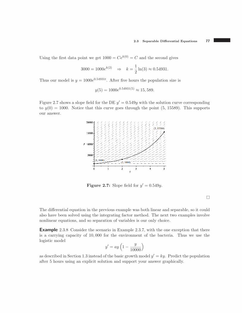
2.3 Separable Differential Equations 77
Using the first data point we get 1000 = Cek(0) = C and the second gives
3000 = 1000ek(2) ⇒ k =1
2ln(3) ≈ 0.54931.
Thus our model is y = 1000e0.54931t. After five hours the population size is
y(5) = 1000e0.54931(5) ≈ 15, 589.
Figure 2.7 shows a slope field for the DE y′ = 0.549y with the solution curve correspondingto y(0) = 1000. Notice that this curve goes through the point (5, 15589). This supportsour answer.
Figure 2.7: Slope field for y′ = 0.549y.
The differential equation in the previous example was both linear and separable, so it couldalso have been solved using the integrating factor method. The next two examples involvenonlinear equations, and so separation of variables is our only choice.
Example 2.3.8 Consider the scenario in Example 2.3.7, with the one exception that thereis a carrying capacity of 10, 000 for the environment of the bacteria. Thus we use thelogistic model
y′ = ay(
1− y
10000
)
as described in Section 1.3 instead of the basic growth model y′ = ky. Predict the populationafter 5 hours using an explicit solution and support your answer graphically.
78 CHAPTER 2 First-order Differential Equations
Solution. We replace the carrying capacity with the parameter N and find the generalsolution to the DE using separation of variables. We use software to perform the calcula-tions.
Step 1:dy
dt= ay
(
1− y
N
)
⇒ 1
y(1− y/N)dy = a dt
Step 2:
∫
1
y(1− y/N)dy =
∫
a dt ⇒ ln y − ln(y −N) = at+ c
Step 3: y =N
1− Ce−atwhere C > 0 is a constant
To find C, consider the generic initial condition y(0) = y0:
y0 = y(0) =N
1− Ce−a(0)⇒ C = 1− N
y0.
After distributing the negative sign in front of the C, we get the general model
y =N
1 + (N/y0 − 1) e−at.
This form is quite nice for understanding the behavior of the logistic model. It is easy tosee that y(0) = N/ (N/y0) = y0 and as t → ∞, y → N , which is just what we want tohappen.
To finish our problem we substitute in y0 = 1000 and N = 10, 000 to get the model
y =10000
1 + 9e−at.
The data point y(2) = 3000 yields
3000 =10000
1 + 9e−2a⇒ a = −1
2ln(7/27) ≈ 0.67496.
Plugging this value of a into the model, we get that after 5 years there will be
y =10000
1 + 9e−0.67496(5)≈ 7645 bacteria.
Figure 2.8 provides a graphical verification of this solution.
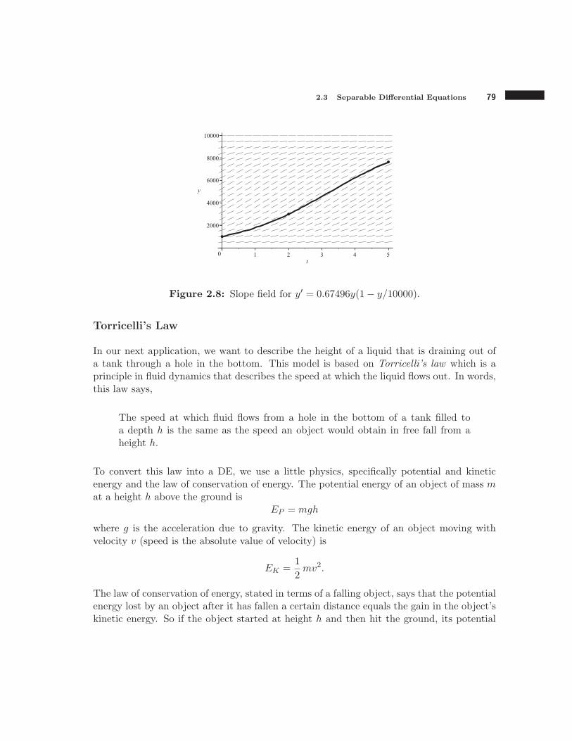
2.3 Separable Differential Equations 79
Figure 2.8: Slope field for y′ = 0.67496y(1− y/10000).
Torricelli’s Law
In our next application, we want to describe the height of a liquid that is draining out ofa tank through a hole in the bottom. This model is based on Torricelli’s law which is aprinciple in fluid dynamics that describes the speed at which the liquid flows out. In words,this law says,
The speed at which fluid flows from a hole in the bottom of a tank filled toa depth h is the same as the speed an object would obtain in free fall from aheight h.
To convert this law into a DE, we use a little physics, specifically potential and kineticenergy and the law of conservation of energy. The potential energy of an object of mass mat a height h above the ground is
EP = mgh
where g is the acceleration due to gravity. The kinetic energy of an object moving withvelocity v (speed is the absolute value of velocity) is
EK =1
2mv2.
The law of conservation of energy, stated in terms of a falling object, says that the potentialenergy lost by an object after it has fallen a certain distance equals the gain in the object’skinetic energy. So if the object started at height h and then hit the ground, its potential
80 CHAPTER 2 First-order Differential Equations
energy went from mgh to 0. If the object started at rest, then its kinetic energy went from0 to 1
2 mv2. Note that we are ignoring any type of drag. Thus we have
mgh =1
2mv2.
Solving this equation for v yieldsv =
√
2gh.
This equation describes the speed at which the liquid drains out. If distance is measuredin m and time in sec, then the units of v are m/sec. Let a represent the area of the holethrough which the liquid drains. Its units are m2. If we multiple a and v, we get
a · v =(
am2)
·(
√
2ghm
sec
)
= a√
2ghm3
sec.
The units indicate that a · v represents the change in volume with respect to time (thederivative of the volume). Let V (t) represent the volume of liquid in the tank at time t.Since the volume is decreasing, we have V ′ = −a
√2gh. Now, a, 2, and g are all constants,
so we can rewrite this equation as
V ′ = −a√
2gh = −a√
2g√h = −k
√h (2.6)
where k = a√2g is a constant.2 Note that in this equation, h represents the height of water
in the tank at time t. Thus h is a function of t. If in addition, fluid is being added at aconstant rate rin, then we get
V ′(t) = rin − k√
h(t) (2.7)
using the rate of accumulation principle.
The problem with equation (2.7) is that it involves two dependent variables, V and h. Inorder to solve this problem we need to relate V to h, which depends on the geometry ofthe tank. For example, in a cylindrical tank with radius R we have
V (t) = πR2h ⇒ V ′ = πR2h′
which yields the DE for hπR2h′ = rin − k
√h. (2.8)
2Determining the value of k is not as simple as measuring the area of the hole and then multiplying itby
√
2g. In real-world situations, the fluid flows out in such a way that the flow-lines narrow, reducing theeffective area of the hole by some contraction coefficient. This coefficient must be experimentially measured.In other words, k must be experimentially measured. See Exercise 2.3.19 for a scenario illustrating how k
could be measured.
2.3 Separable Differential Equations 81
In general, if A(h) is the cross-sectional area of the tank as a function of h then we canwrite V ′ = A(h)h′ (because for a small change in height dh the change in volume would bedV = A(h)dh, then divide by dt). The differential equation for h becomes
A(h)h′ = rin − k√h (2.9)
Using these models we can predict when a tank will empty (that is, when h(t) = 0) asillustrated in the next example.
Example 2.3.9 Consider a cylindrical can of soda with a small hole punched in the bottom.The radius of the can is 1 in and initially the soda in the can is 8 in deep. The soda beginto drain and after 10 sec the soda is 5 in deep. When will the can be empty?
Solution. We use the model in equation (2.8). We have R = 1, and there is no fluidcoming into the can so rin = 0. Thus the model simplifies to
h′ = −k
π
√h
This DE is separable. Using the method of separation of variables or software, a generalsolution is
h =
(
− k
2πt+ C
)2
To find the values of C and k, we use the conditions h(0) = 8 and h(10) = 5. The firstcondition gives 8 = C2 so C =
√8. The second condition gives
5 =
(
− k
2π(10) +
√8
)2
⇒ k =π
5
(√8−
√5)
≈ 0.3722.
This yields the specific solution
h =
[
− 1
10
(√8−
√5)
t+√8
]2
≈ h = (2.8284− 0.059236t)2.
Setting h = 0 to find when the can is empty, we get
t =2.8284
0.059236≈ 47.75 sec.
82 CHAPTER 2 First-order Differential Equations
Exercises
Determine whether or not each equation is separable.
2.3.1 x′ + 2x = e−t
2.3.2 x′ + 2x = 1
2.3.3 x′ =x+ 1
t+ 1
2.3.4 x′ = sin tcos x
Solve each below by the method of separation of variables:
2.3.5 x′ =x
t
2.3.6 x′ =t
x
2.3.7 x′ = x+ 5
2.3.8 x′ = 3x− 2
2.3.9 x′ = x cos(t)
2.3.10 x′ = (1 + t)(2 + x)
Solve each of the following initial-value problems:
2.3.11 y′ = y + 1, y(0) = 2
2.3.12 y′ = ty, y(0) = 3
2.3.13 x′ = x cos(t), x(0) = 1
2.3.14 x′ = (1 + t)(2 + x), x(0) = −1
2.3.15 P ′ = 2P (1− P ), P (0) = 1/2
2.3.16 (Population growth) A population P is growing according to the growth law dPdt = rP .
Time t is measured in years. If the population is initially 100, and after 1 year the population is150, how many will there be after 2 years? Hint: solve the differential equation for P as a functionof t. Then use the two conditions P (0) = 100 and P (1) = 150 to determine r and the integrationconstant. What happens to the population in the long term?
2.3.17 (Population growth) Repeat the previous problem, but this time assume the growth lawdPdt = rP (1− P/300). What happens to the population in the long term?
2.4 Numerical methods for first-order equations 83
2.3.18 (Falling bodies) In Section 1.1 we derived a DE to model a falling piece of crumpled paper.This model stated in terms of the velocity v is
mv′ = −mg − cv
where g = 9.8m/sec2 is the acceleration due to gravity, m is the mass in kg, and c is the constantof proportionality used to describe the force due to air resistance.
a. Assuming that both m and c are positive, find the general solution to the differential equationmv′ = −mg − cv for v as a function of t. (Hint: first show that dv
g+ c
mv = −dt.)
b. Find limt→∞ v(t). This is called the terminal velocity of the falling body.
c. Suppose that a body with mass 1kg has a teminal velocity of −20m/sec. Find the value of c.
d. According to this model, does the body ever actually reach terminal velocity? Briefly explainwhy or why not.
e. How long does it take the body from part c. to get within 1% of terminal velocity?
2.3.19 Suppose water is draining out of a tank through a hole in the bottom. At time t = 1 sec,the height of the water in the tank was 0.4 m and the volume of water in the tank was 1.1 m3. Attime t = 1.5 sec, the height was 0.38 m and the volume was 1 m3. Use this information to estimatethe value of k in equation (2.6). (Hint: V ′ ≈ (change in V )/(change in t). Use an approximationof h in the right-hand side.)
2.3.20 Use equation (2.9) to find the model for h for the following types of tanks.
a. A cubical tank with sides of length l.
b. A conical tank of height b and radius R.
c. A spherical tank of radius R.
2.3.21 In Example 2.3.9 we solved the DE h′ = − kπ
√h where k ≈ 0.3722 and got the specific
solution h = (2.8284− 0.059236t)2. Show that this solution is not valid for t > 47.75. (Hint: Bothsides of the DE must have the same sign.)
2.4 Numerical methods for first-order equations
In Section 1.2 we saw Euler’s method, which is a numerical method for approximating asolution to an IVP without having to find an explicit solution. Euler’s method is relativelyeasy to perform, but we have seen that the method can yield rather large errors, especiallyif a small step size is used. Fortunately, better numerical methods exist. These methodsbuild on the ideas of Euler’s method and result in more complex algorithms. The increasein complexity is more than made up for in by an increase in speed and accuracy. In thissection we discuss and compare two such methods.

84 CHAPTER 2 First-order Differential Equations
Order of convergence
One way of comparing different numerical methods is with order of convergence. The nextexample illustrates some ideas related to the order of convergence.
Example 2.4.1 Consider the DE y′ = y − x with the initial condition y(0) = 0.5. Theexact solution to this IVP is y = −0.5ex+x+1 (the reader should verify this) which yieldsthe value y(2) = −0.69453. Use Euler’s method with step sizes of ∆x = 0.5, 0.1, 0.01, and0.001 to approximate the value of y(2).
Solution. Partial tables of the calculations from Euler’s method are shown below.
∆x = 0.5 ∆x = 0.1 ∆x = 0.01 ∆x = 0.001
xi yi xi yi xi yi xi yi
0.0 0.5 0.0 0.5 0.0 0.5 0.0 0.5
0.5 0.75 0.1 0.55 0.01 0.505 0.001 0.5005
0.0 0.875 0.2 0.595 0.02 0.50995 0.002 0.501
1.5 0.8125 1.9 −0.15795 1.99 −0.63179 1.999 −0.68815
2.0 0.46875 2.0 −0.36375 2.0 −0.65801 2.0 −0.69084
For ∆x = 0.1, for example, we get the approximation y(2) ≈ −0.36375. The differencebetween the exact value and the approximate value,
|−0.69453− (−0.36375)| = 0.33078
is called the global truncation error. The global truncation errors for ∆x = 0.05, ∆x = 0.01,and ∆x = 0.001 are 1.16328, 0.03652, and 0.00369, respectively.
Notice that in this example, as the step size gets smaller, the global truncation error alsogets smaller. We could also say that as the step size gets smaller, the approximate solutionconverges to the exact solution. The order of convergence helps quantify this idea.
Definition 2.4.1 The order of convergence of a numerical method is said to be kif the global truncation error is divided by approximately Mk when the step sizeis divided by M (for a sufficiently small step size). We also say the method is kthorder convergent.
2.4 Numerical methods for first-order equations 85
In Example 2.4.1, note that when the step size went from ∆x = 0.1 to ∆x = 0.01, thestep size was divided by 10. The global truncation error went from 0.33078 to 0.03652,showing that the error was divided by about 101. When the step size went from ∆x = 0.01to ∆x = 0.001, we got similar results. This illustrates that Euler’s method is 1st orderconvergent.
However, note that when the step size went from ∆x = 0.5 to ∆x = 0.1, the step size wasdivided by 5 but the error was divided by about 3.5 (decreasing from 1.16328 to 0.33078).This shows the necessity of the qualifer “for a sufficiently small step size” in the definitionof order of convergence. How small the step size needs to be is not easy to determine.
This example illustrates that in practical terms, 1st order convergent means that when thestep size is small enough, reducing it by dividing by 10 yields one more digit of accuracy.Second order convergent means that the same reduction in step size will divide the error by102 = 100, meaning two more digits of accuracy. In general, kth order convergent means kmore digits of accuracy.
Runge-Kutta methods
In the early 1900’s, the German mathematicians C. Runge and M.W. Kutta developed twonumerical methods that are widely used to this day. The first of these methods is calledthe Runge-Kutta second order method, or RK2 method for short. It is also known as themodified Euler method. This is a second order convergent method that is based on similarlogic as Euler’s method.
RK2 for First-Order IVP’s
Given a differential equation y′ = f(x, y) and an initial condition y(x0) = y0,calculate the points (x1, y1) , . . . , (xn, yn) using
k1 = f (xi, yi)∆x
k2 = f
(
xi +1
2∆x, yi +
1
2k1
)
∆x
xi+1 = xi +∆x
yi+1 = yi + k2
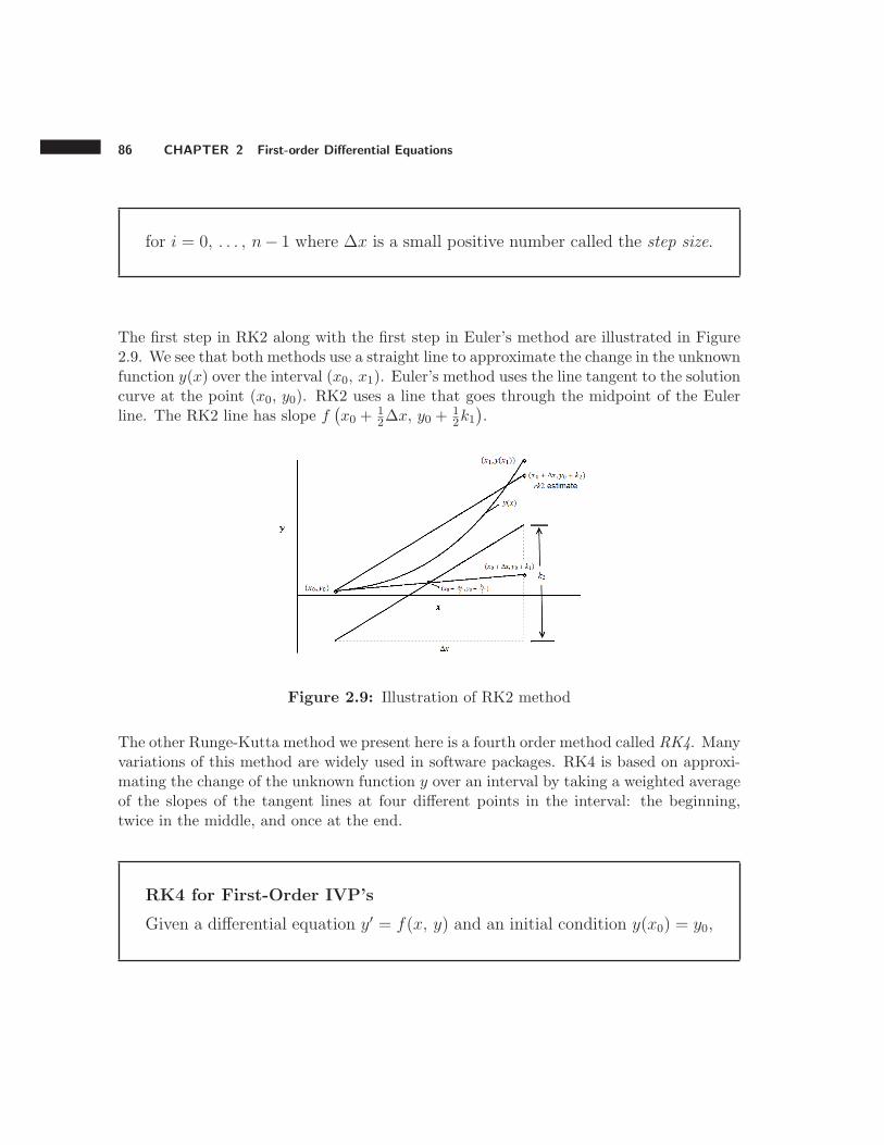
86 CHAPTER 2 First-order Differential Equations
for i = 0, . . . , n− 1 where ∆x is a small positive number called the step size.
The first step in RK2 along with the first step in Euler’s method are illustrated in Figure2.9. We see that both methods use a straight line to approximate the change in the unknownfunction y(x) over the interval (x0, x1). Euler’s method uses the line tangent to the solutioncurve at the point (x0, y0). RK2 uses a line that goes through the midpoint of the Eulerline. The RK2 line has slope f
(
x0 +12∆x, y0 +
12k1
)
.
Figure 2.9: Illustration of RK2 method
The other Runge-Kutta method we present here is a fourth order method called RK4. Manyvariations of this method are widely used in software packages. RK4 is based on approxi-mating the change of the unknown function y over an interval by taking a weighted averageof the slopes of the tangent lines at four different points in the interval: the beginning,twice in the middle, and once at the end.
RK4 for First-Order IVP’s
Given a differential equation y′ = f(x, y) and an initial condition y(x0) = y0,
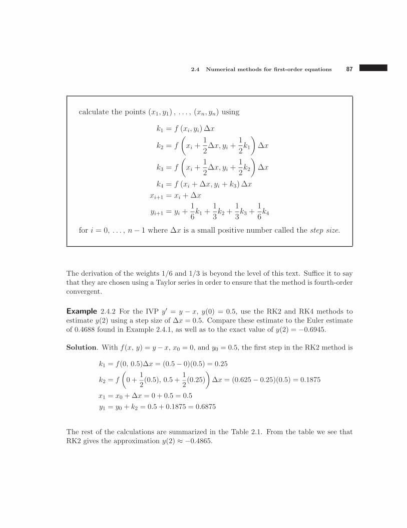
2.4 Numerical methods for first-order equations 87
calculate the points (x1, y1) , . . . , (xn, yn) using
k1 = f (xi, yi)∆x
k2 = f
(
xi +1
2∆x, yi +
1
2k1
)
∆x
k3 = f
(
xi +1
2∆x, yi +
1
2k2
)
∆x
k4 = f (xi +∆x, yi + k3)∆x
xi+1 = xi +∆x
yi+1 = yi +1
6k1 +
1
3k2 +
1
3k3 +
1
6k4
for i = 0, . . . , n− 1 where ∆x is a small positive number called the step size.
The derivation of the weights 1/6 and 1/3 is beyond the level of this text. Suffice it to saythat they are chosen using a Taylor series in order to ensure that the method is fourth-orderconvergent.
Example 2.4.2 For the IVP y′ = y − x, y(0) = 0.5, use the RK2 and RK4 methods toestimate y(2) using a step size of ∆x = 0.5. Compare these estimate to the Euler estimateof 0.4688 found in Example 2.4.1, as well as to the exact value of y(2) = −0.6945.
Solution. With f(x, y) = y− x, x0 = 0, and y0 = 0.5, the first step in the RK2 method is
k1 = f(0, 0.5)∆x = (0.5− 0)(0.5) = 0.25
k2 = f
(
0 +1
2(0.5), 0.5 +
1
2(0.25)
)
∆x = (0.625− 0.25)(0.5) = 0.1875
x1 = x0 +∆x = 0 + 0.5 = 0.5
y1 = y0 + k2 = 0.5 + 0.1875 = 0.6875
The rest of the calculations are summarized in the Table 2.1. From the table we see thatRK2 gives the approximation y(2) ≈ −0.4865.

88 CHAPTER 2 First-order Differential Equations
x y k1 k2 y + k2
0 0.5 0.25 0.1875 0.6875
0.5 0.6875 0.09375 −0.007813 0.6797
1.0 0.6797 −0.1602 −0.0003780 0.3545
1.5 0.3545 −0.5728 −0.8410 −0.4865
2.0 −0.4865
Table 2.1: RK2 method for y′ = y − x
The first step in the RK4 method is
k1 = f(0, 0.5)∆x = (0.5− 0)(0.5) = 0.25
k2 = f
(
0 +1
2(0.5), 0.5 +
1
2(0.25)
)
∆x = (0.625− 0.25)(0.5) = 0.1875
k3 = f
(
0 +1
2(0.5), 0.5 +
1
2(0.1875)
)
∆x = (0.5938− 0.25)(0.5) = 0.1719
k4 = f(0 + 0.5, 0.5 + 0.1719)∆x = (0.67188− 0.5)(0.5) = 0.08594
x1 = x0 +∆x = 0 + 0.5 = 0.5
y1 = y0 +1
6(0.25) +
1
3(0.1875) +
1
3(0.1719) +
1
6(0.0859) = 0.6758
The rest of the values are summarized in the Table 2.2. From the table we see that RK4gives the approximation y(2) ≈ −0.6920.
x y k1 k2 k3 k4 y + 16k1 + · · ·+ 1
6k4
0 0.5 0.25 0.1875 0.1719 0.0859 0.6758
0.5 0.6758 0.0879 −0.0151 −0.0409 −0.1826 0.6413
1.0 0.6413 −0.1793 −0.3492 −0.3916 −0.6252 0.2603
1.5 0.2603 −0.6198 −0.8998 −0.9698 −1.3547 −0.6920
2.0 −0.6920
Table 2.2: RK4 method for y′ = y − x
These results are summarized in Table 2.3. Clearly the estimates are better with higherorder methods.
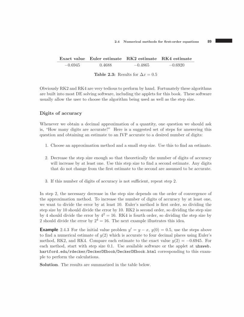
2.4 Numerical methods for first-order equations 89
Exact value Euler estimate RK2 estimate RK4 estimate
−0.6945 0.4688 −0.4865 −0.6920
Table 2.3: Results for ∆x = 0.5
Obviously RK2 and RK4 are very tedious to perform by hand. Fortunately these algorithmsare built into most DE solving software, including the applets for this book. These softwareusually allow the user to choose the algorithm being used as well as the step size.
Digits of accuracy
Whenever we obtain a decimal approximation of a quantity, one question we should askis, “How many digits are accurate?” Here is a suggested set of steps for answering thisquestion and obtaining an estimate to an IVP accurate to a desired number of digits:
1. Choose an approximation method and a small step size. Use this to find an estimate.
2. Decrease the step size enough so that theoretically the number of digits of accuracywill increase by at least one. Use this step size to find a second estimate. Any digitsthat do not change from the first estimate to the second are assumed to be accurate.
3. If this number of digits of accuracy is not sufficient, repeat step 2.
In step 2, the necessary decrease in the step size depends on the order of convergence ofthe approximation method. To increase the number of digits of accuracy by at least one,we want to divide the error by at least 10. Euler’s method is first order, so dividing thestep size by 10 should divide the error by 10. RK2 is second order, so dividing the step sizeby 4 should divide the error by 42 = 16. RK4 is fourth order, so dividing the step size by2 should divide the error by 24 = 16. The next example illustrates this idea.
Example 2.4.3 For the initial value problem y′ = y − x, y(0) = 0.5, use the steps aboveto find a numerical estimate of y(2) which is accurate to four decimal places using Euler’smethod, RK2, and RK4. Compare each estimate to the exact value y(2) = −0.6945. Foreach method, start with step size 0.1. Use available software or the applet at uhaweb.
hartford.edu/rdecker/DeckerDEbook/DeckerDEbook.html corresponding to this exam-ple to perform the calculations.
Solution. The results are summarized in the table below.
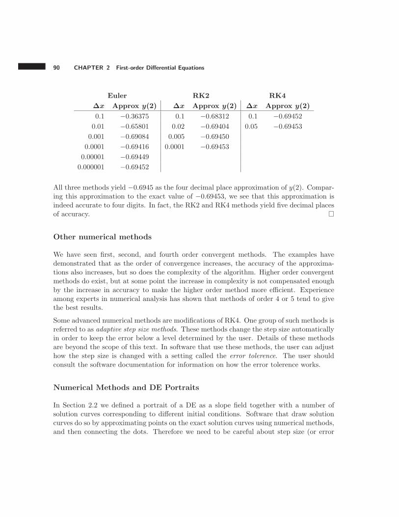
90 CHAPTER 2 First-order Differential Equations
Euler RK2 RK4
∆x Approx y(2) ∆x Approx y(2) ∆x Approx y(2)
0.1 −0.36375 0.1 −0.68312 0.1 −0.69452
0.01 −0.65801 0.02 −0.69404 0.05 −0.69453
0.001 −0.69084 0.005 −0.69450
0.0001 −0.69416 0.0001 −0.69453
0.00001 −0.69449
0.000001 −0.69452
All three methods yield −0.6945 as the four decimal place approximation of y(2). Compar-ing this approximation to the exact value of −0.69453, we see that this approximation isindeed accurate to four digits. In fact, the RK2 and RK4 methods yield five decimal placesof accuracy.
Other numerical methods
We have seen first, second, and fourth order convergent methods. The examples havedemonstrated that as the order of convergence increases, the accuracy of the approxima-tions also increases, but so does the complexity of the algorithm. Higher order convergentmethods do exist, but at some point the increase in complexity is not compensated enoughby the increase in accuracy to make the higher order method more efficient. Experienceamong experts in numerical analysis has shown that methods of order 4 or 5 tend to givethe best results.
Some advanced numerical methods are modifications of RK4. One group of such methods isreferred to as adaptive step size methods. These methods change the step size automaticallyin order to keep the error below a level determined by the user. Details of these methodsare beyond the scope of this text. In software that use these methods, the user can adjusthow the step size is changed with a setting called the error tolerence. The user shouldconsult the software documentation for information on how the error tolerence works.
Numerical Methods and DE Portraits
In Section 2.2 we defined a portrait of a DE as a slope field together with a number ofsolution curves corresponding to different initial conditions. Software that draw solutioncurves do so by approximating points on the exact solution curves using numerical methods,and then connecting the dots. Therefore we need to be careful about step size (or error

2.4 Numerical methods for first-order equations 91
tolerance) so that we get an accurate portrait. We can get idea of how accurate the portraitis by trying a smaller step size. If the portrait does not change much, then we assume theportait is accurate.
Example 2.4.4 Draw a portrait of the DE x′ = x+t over the region −2 ≤ t ≤ 2, −2 ≤ x ≤ 2using available software. Use different step sizes to verify the phase portrait is accurate.
Solution. Figure 2.4.4 shows portraits generated with Euler’s method with step sizes of0.5, 0.05, and 0.005.
(a) ∆t = 0.5 (b) ∆t = 0.05
(c) ∆t = 0.005
Figure 2.10: Portraits of x′ = x+ t using Euler’s method
Notice that the portrait with step size 0.5 is quite a bit different than then other portraits.The solution curves in this portrait touch, which violates Theorem 2.3. Thus we concludethat this portrait is very inaccurate. The portraits with step sizes 0.05 and 0.005 are verysimilar, so we conclude that they are sufficiently accurate.
Exercises
2.4.1 For the IVP y′ = −2y, y(0) = 1, estimate the value of y(2) by making a table of values usingRK2 with 4 steps and step size ∆t = 0.5 (do the work without using built-in computer or calculatormethods, as in example 2.4.2). Repeat with RK4. Compare to the exact solution (which you can
92 CHAPTER 2 First-order Differential Equations
calculate using separation of variables, or computer algebra) and give the amount of error for eachmethod.
2.4.2 For the IVP x′ = −x+ et, x(0) = 2, estimate the value of x(1) by making a table of valuesusing RK2 with 4 steps and step size ∆t = 0.25 (do the work without using built-in computer orcalculator methods, as in example 2.4.2). Repeat with RK4. Compare to the exact solution (whichyou can calculate using the integrating factor method, or computer algebra) and give the amountof error for each method.
For each I.V.P. 3 - 6, estimate the value of the dependent variable accurate to three sig-nificant digits at the point where the independent variable is equal to 5. First use Euler’smethod, then repeat using either fourth-order Runga-Kutta or an adaptive step size RKmethod (as on the TI-89 calculator). Use a computer or calculator built-in method, or alterthe first-order applet at .
2.4.3 y′ = −y + sin(t), y(0) = 1.
2.4.4 x′ = x2 − t, x(0) = 0.
2.4.5 y′ = −0.1xy, y(0) = 4.
2.4.6 p′ = p(1− p) + 0.5 cos(t), p(0) = 0.
Create accurate phase portraits of each differential equation 7 - 10, and include in the phaseportrait the solution curve corresponding to the initial condition given. They are the sameas the previous four problems, and you can use the same technology you used there.
2.4.7 y′ = −y + sin(t), y(0) = 1.
2.4.8 x′ = x2 − t, x(0) = 0.
2.4.9 y′ = −0.1xy, y(0) = 4.
2.4.10 p′ = p(1− p) + 0.5 cos(t), p(0) = 0.
2.5 Autonomous first-order equations and bifurcations
Differential equations always involve a dependent and at least one independent variable. Inthe DE
y′ = x+ y,
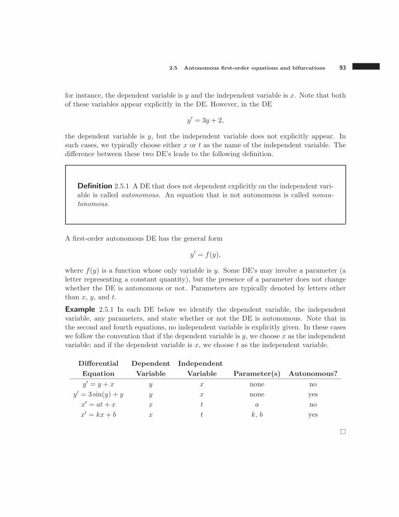
2.5 Autonomous first-order equations and bifurcations 93
for instance, the dependent variable is y and the independent variable is x. Note that bothof these variables appear explicitly in the DE. However, in the DE
y′ = 3y + 2,
the dependent variable is y, but the independent variable does not explicitly appear. Insuch cases, we typically choose either x or t as the name of the independent variable. Thedifference between these two DE’s leads to the following definition.
Definition 2.5.1 A DE that does not dependent explicitly on the independent vari-able is called autonomous. An equation that is not autonomous is called nonau-
tonomous.
A first-order autonomous DE has the general form
y′ = f(y),
where f(y) is a function whose only variable is y. Some DE’s may involve a parameter (aletter representing a constant quantity), but the presence of a parameter does not changewhether the DE is autonomous or not. Parameters are typically denoted by letters otherthan x, y, and t.
Example 2.5.1 In each DE below we identify the dependent variable, the independentvariable, any parameters, and state whether or not the DE is autonomous. Note that inthe second and fourth equations, no independent variable is explicitly given. In these caseswe follow the convention that if the dependent variable is y, we choose x as the independentvariable; and if the dependent variable is x, we choose t as the independent variable.
Differential Dependent Independent
Equation Variable Variable Parameter(s) Autonomous?
y′ = y + x y x none no
y′ = 3 sin(y) + y y x none yes
x′ = at+ x x t a no
x′ = kx+ b x t k, b yes

94 CHAPTER 2 First-order Differential Equations
Properties of autonomous DE’s
The fact that the right-hand side of the first-order autonomous DE y′ = f(y) dependsonly on y and not the independent variable (which we will assume to be x) results in somespecial properties. Below we describe three such properties.
1. Separability A first-order autonomous DE is always separable because
y′ = f(y) ⇒ dy
dx= f(y) ⇒
∫
1
f(y)dy =
∫
dx.
This, however, does not mean that an explicit solution in terms of elementary func-tions is always obtainable.
2. Slope Field Along a horizontal line y = b, where b is a constant, the slope marks ina slope field are identical. For example, consider the autonomous DE y′ = y(1 − y).Along the line y = 2, for instance, all the slope marks have slope 2(1 − 2) = −1.A slope field of this DE is shown in Figure 2.11. Notice how the slope marks areidentical along each “row” of marks.
Figure 2.11: Slope field for y′ = y(1− y)
3. Constant Solutions The constant function y(x) = a is a solution to the DE y′ =f(y) if f(a) = 0. This is easily verified since the derivative of a constant function is0. Constant solutions are also called equilibrium solutions and fixed points. Constantsolutions do not always appear when a general solution is found using techniques suchas separation of variables, so constant solutions must be found separately. Luckilythis is relatively easy. All we need to do is set f(y) = 0 and solve for y.
2.5 Autonomous first-order equations and bifurcations 95
Example 2.5.2 Use separation of variables to find a general solution to each DE below.Also find any constant solution. For each constant solution, state whether or not it is partof the general solution that comes from separation of variables.
1. y′ = ky
2. y′ = ky(1− y)
3. y′ = e−y(1− y)
Solution. We omit most of the details of separation of variables. The reader may refer toSection 2.3 for a refresher on this technique.
1. Separation of variables yields the general solution y = Cekx. To find constant so-lutions, we set ky = 0. This results in the constant solution y = 0. The constantsolution corresponds to C = 0 in the general solution.
2. Separation of variables gives
∫
1
y(1− y)dy =
∫
k dx ⇒ ln(y)− ln(1− y) = kx+ c ⇒ y =Cekx
1 + Cekx
where C = ec. For constant solutions we set ky(1 − y) = 0, resulting in y = 0 andy = 1. The solution y = 0 corresponds to C = 0 in the general solution, but the y = 1constant solution does not correspond to any finite value of C.
3. Separation of variables gives
∫
ey
1− ydy =
∫
dx.
The integral on the left cannot be evaluated in terms of elementary functions, so noexplicit general solution is possible. Setting e−y(1 − y) = 0, we get the constantsolution y = 1.
Graphical behavior of a solution
The constant solution(s) to an automonous DE can tell us a great deal about the graphicalbehavior of a solution to the DE. To obtain this information, we use the idea of a zero ofa function. A zero of a function f(x) is a number a such that f(a) = 0. We also use thefollowing theorem, which is a result of the Intermediate Value Theorem of Calculus.
96 CHAPTER 2 First-order Differential Equations
Theorem 2.4 If a function f(x) is continuous, and if f(x) has zeros at points x = a andx = b and no other zeros between a and b, then f(x) must be purely positive (f(x) > 0) orpurely negative (f(x) < 0) for a < x < b. Similarly, if f(x) has a zero x = a but no otherzero for x > a, then f(x) must be purely positive or purely negative for x > a. A similarresult holds if f(x) has no other zero for x < a.
In the automonous DE y′ = f(y), the zeros of f(y) are the constant solutions. According toTheorem 2.4, for y between two constant solutions, f(y) must be purely positive or purelynegative. The same is true for y above the largest, or below the smallest constant solution.This is important for two reasons:
1. The sign of f(y) is the same as the sign of y′.
2. If y′ is positive, then the graph of y(x) is increasing. Likewise, if y′ is negative, thenthe graph of y(x) is decreasing.
This result can be used to determine intervals over which the solution curves are increasing,and intervals on which the curves are decreasing. The next example illustrates this.
Example 2.5.3 For the differential equation y′ = y(y−2)2(y−4), find all constant solutions.Then determine on which intervals of y the solution curves are increasing, and on whichintervals the solution curves are decreasing. From that information sketch a DE portrait.
Solution. Setting f(y) = y(y − 2)2(y − 4) = 0 we get the constant solutions y = 0, y = 2,and y = 4. This divides the real number line into four intervals:
y < 0, 0 < y < 2, 2 < y < 4, and y > 4.
Since we know that the function f(y) must be purely positive or purely negative on eachinterval, we can pick one y value from each interval and substitute it into f(y) to determinewhether f(y) is positive or negative on that interval.
For example, in the interval y < 0, we can choose y = −1 and evaluate
f(−1) = −1(−1− 2)2(−1− 4) = 45,
which is positive. Thus we know that solution curves are increasing for y < 0. Results forthe other intervals are shown in Table 2.4.
Figure 2.12 shows a DE portrait drawn with software. Notice that the behavior of solutioncurves agrees with the conclusions in Table 2.4 and that the horizontal curves correspondto constant solutions.

2.5 Autonomous first-order equations and bifurcations 97
Interval y chosen f(y) Inc/Dec?
y < 0 −1 45 Increasing
0 < y < 2 1 −3 Decreasing
2 < y < 4 3 −3 Decreasing
y > 4 5 45 Increasing
Table 2.4: y intervals for y′ = y(y − 2)2(y − 4)
Figure 2.12: DE portrait for y′ = y(y − 2)2(y − 4)
Analyzing the solution curves in Figure 2.12, we make the following thee observations:
1. Curves “near” the constant solution y = 0 approach this constant solution as x getslarger. In such a case we say that y = 0 attracts nearby solution curves.
2. Near the constant solution y = 4, solution curves move away as x gets larger. In thiscase we say that y = 4 repels nearby solution curves.
3. For the constant solution y = 2, solution curves just above y = 2 are attracted, andsolution curves just below y = 2 are repelled.
These observations lead to the following definition.
98 CHAPTER 2 First-order Differential Equations
Definition 2.5.2 A constant solution that attracts nearby solution curves is calleda sink. A constant solution that repels nearby solution curves is called a source. Aconstant solution that attracts solution curves on one side and repels them on theother side is called a node. We say that sinks are stable, sources are unstable, andnodes are semi-stable.
We can display information about an autonomous DE’s constant solutions, and the stablitytypes of those solutions, using a graphical tool called a phase line. A phase line is a verticalnumber line with the constant solutions (or fixed points) marked on it. Between the fixedpoints, arrows are used to indicate which direction the solution curves move as x increases(an up arrow for increasing and a down arrow for decreasing).
We can use the phase line to easily determine the stability of a constant solution.
• If the arrows on either side of a constant solution are pointing toward the constantsolution, the solution is a sink.
• If the arrows are pointing away form the constant solution, the solution is a source.
• If one arrow points toward and one away from the constant solution, the solution isa node.
The next example illustrates these ideas.
Example 2.5.4 Sketch a phase line for the DE y′ = y(y−2)2(y−4) from Example 2.5.3, anduse the phase line to classify the constant solutons as to their stability type (sink, source,or node). Also display a DE portrait next to the phase line. Finally, describe the long-termbehaviors of the solutions corresponding to different values of the initial condition y(0).
Solution. From Table 2.4, we see that the phase line should have the points y = 0, y = 2,and y = 4 marked as constant solutions. There should be up arrows for y > 4 and y < 0,and down arrows for 0 < y < 2 and 2 < y < 4. Figure 2.5.4 shows the phase line next to aDE portrait. From both the phase line and the portrait, we see that y = 0 is a sink, y = 4is a source, and y = 2 is a node.
We can also see that if y(0) > 4 then y → ∞ as x increases, if 2 ≤ y(0) < 4 then y → 2,and if y(0) < 2 then y → 0. If y(0) equals any of the constant solutions, then y(t) does notchange.
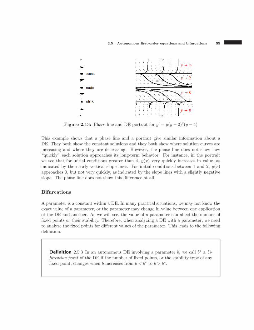
2.5 Autonomous first-order equations and bifurcations 99
Figure 2.13: Phase line and DE portrait for y′ = y(y − 2)2(y − 4)
This example shows that a phase line and a portrait give similar information about aDE. They both show the constant solutions and they both show where solution curves areincreasing and where they are decreasing. However, the phase line does not show how“quickly” each solution approaches its long-term behavior. For instance, in the portraitwe see that for initial conditions greater than 4, y(x) very quickly increases in value, asindicated by the nearly vertical slope lines. For initial conditions between 1 and 2, y(x)approaches 0, but not very quickly, as indicated by the slope lines with a slightly negativeslope. The phase line does not show this difference at all.
Bifurcations
A parameter is a constant within a DE. In many practical situations, we may not know theexact value of a parameter, or the parameter may change in value between one applicationof the DE and another. As we will see, the value of a parameter can affect the number offixed points or their stability. Therefore, when analyzing a DE with a parameter, we needto analyze the fixed points for different values of the parameter. This leads to the followingdefinition.
Definition 2.5.3 In an autonomous DE involving a parameter b, we call b∗ a bi-
furcation point of the DE if the number of fixed points, or the stability type of anyfixed point, changes when b increases from b < b∗ to b > b∗.
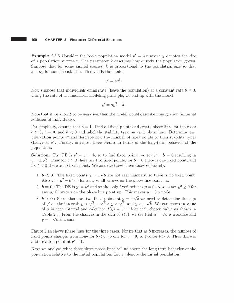
100 CHAPTER 2 First-order Differential Equations
Example 2.5.5 Consider the basic population model y′ = ky where y denotes the sizeof a population at time t. The parameter k describes how quickly the population grows.Suppose that for some animal species, k is proportional to the population size so thatk = ay for some constant a. This yields the model
y′ = ay2.
Now suppose that individuals emmigrate (leave the population) at a constant rate b ≥ 0.Using the rate of accumulation modeling principle, we end up with the model
y′ = ay2 − b.
Note that if we allow b to be negative, then the model would describe immigration (externaladdition of individuals).
For simplicity, assume that a = 1. Find all fixed points and create phase lines for the casesb > 0, b = 0, and b < 0 and label the stability type on each phase line. Determine anybifurcation points b∗ and describe how the number of fixed points or their stability typeschange at b∗. Finally, interpret these results in terms of the long-term behavior of thepopulation.
Solution. The DE is y′ = y2 − b, so to find fixed points we set y2 − b = 0 resulting iny = ±
√b. Thus for b > 0 there are two fixed points, for b = 0 there is one fixed point, and
for b < 0 there is no fixed point. We analyze these three cases separately.
1. b < 0 : The fixed points y = ±√b are not real numbers, so there is no fixed point.
Also y′ = y2 − b > 0 for all y so all arrows on the phase line point up.
2. b = 0 : The DE is y′ = y2 and so the only fixed point is y = 0. Also, since y2 ≥ 0 forany y, all arrows on the phase line point up. This makes y = 0 a node.
3. b > 0 : Since there are two fixed points at y = ±√b we need to determine the sign
of y′ on the intervals y >√b, −
√b < y <
√b, and y < −
√b. We can choose a value
of y in each interval and calculate f(y) = y2 − b at each chosen value as shown inTable 2.5. From the changes in the sign of f(y), we see that y =
√b is a source and
y = −√b is a sink.
Figure 2.14 shows phase lines for the three cases. Notice that as b increases, the number offixed points changes from none for b < 0, to one for b = 0, to two for b > 0. Thus there isa bifurcation point at b∗ = 0.
Next we analyze what these three phase lines tell us about the long-term behavior of thepopulation relative to the initial population. Let y0 denote the initial population.
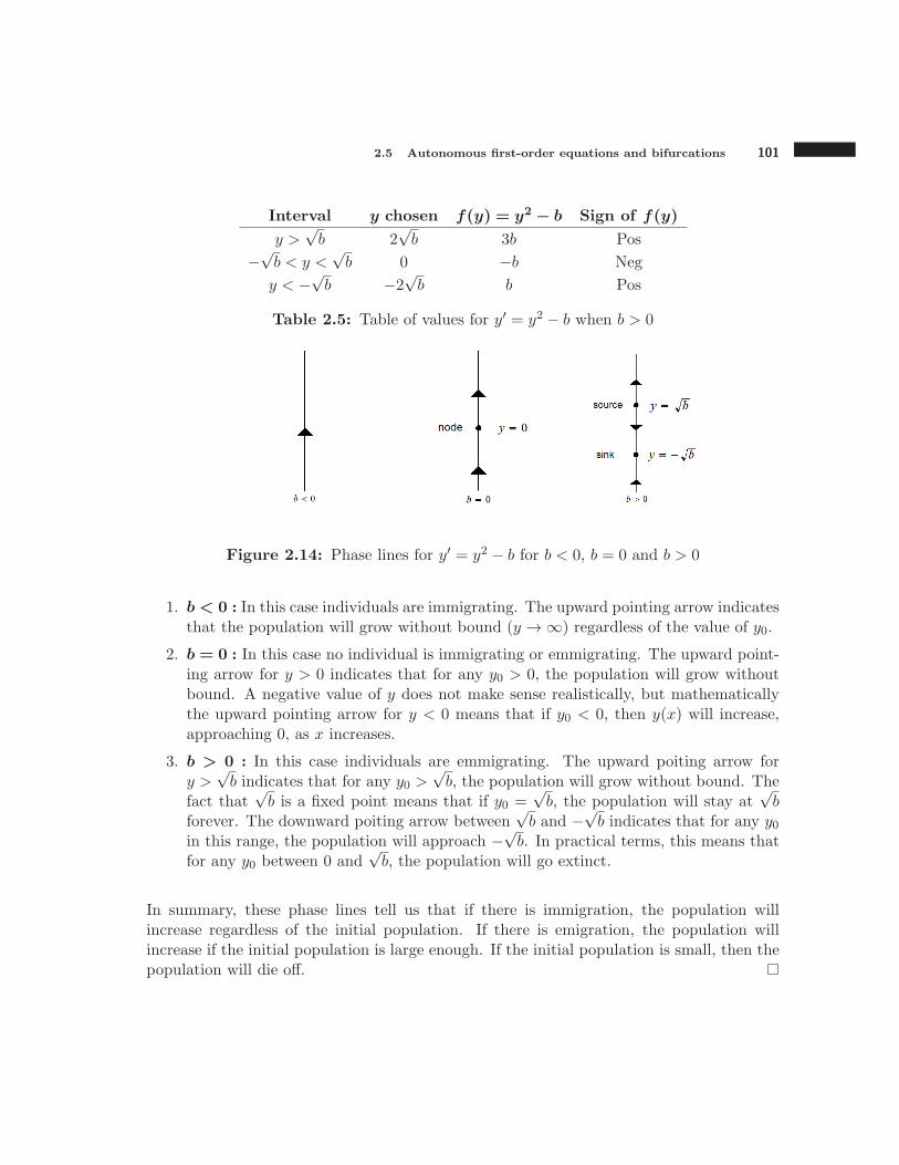
2.5 Autonomous first-order equations and bifurcations 101
Interval y chosen f(y) = y2− b Sign of f(y)
y >√b 2
√b 3b Pos
−√b < y <
√b 0 −b Neg
y < −√b −2
√b b Pos
Table 2.5: Table of values for y′ = y2 − b when b > 0
Figure 2.14: Phase lines for y′ = y2 − b for b < 0, b = 0 and b > 0
1. b < 0 : In this case individuals are immigrating. The upward pointing arrow indicatesthat the population will grow without bound (y → ∞) regardless of the value of y0.
2. b = 0 : In this case no individual is immigrating or emmigrating. The upward point-ing arrow for y > 0 indicates that for any y0 > 0, the population will grow withoutbound. A negative value of y does not make sense realistically, but mathematicallythe upward pointing arrow for y < 0 means that if y0 < 0, then y(x) will increase,approaching 0, as x increases.
3. b > 0 : In this case individuals are emmigrating. The upward poiting arrow fory >
√b indicates that for any y0 >
√b, the population will grow without bound. The
fact that√b is a fixed point means that if y0 =
√b, the population will stay at
√b
forever. The downward poiting arrow between√b and −
√b indicates that for any y0
in this range, the population will approach −√b. In practical terms, this means that
for any y0 between 0 and√b, the population will go extinct.
In summary, these phase lines tell us that if there is immigration, the population willincrease regardless of the initial population. If there is emigration, the population willincrease if the initial population is large enough. If the initial population is small, then thepopulation will die off.

102 CHAPTER 2 First-order Differential Equations
Bifurcation diagrams
Figure 2.14 tells the story of how the fixed points of y′ = y2 − b and their stability typesdepend on the parameter b. We can expand this figure into a type of graph called abifurcation diagram, giving and even more detailed representation of a bifurcation.
A bifurcation diagram consists of a number of phase lines placed next to each other, eachcorresponding to a different value of the parameter. The stable fixed points are thenconnected with a solid line, showing how the stable fixed points change as the parameterchanges. Similarly the unstable fixed points are connected with a dotted or dashed line. Abifurcation diagram for the DE y′ = y2 − b in shown in Figure 2.15.
Figure 2.15: Bifurcation diagram for y′ = y2 − b
The important components of the bifurcation diagram in Figure 2.15 include:
• The horizontal axis denotes values of the parameter b. The vertical axis denotes thevalue of the equilibrium solutions (or fixed points) corresponding to each value of b.
• The first quadrant contains a graph of y =√b. This is because for b > 0, one of the
fixed points is√b. This curve is dashed to indicate that this fixed point is unstable.
• The fourth quadrant contains a graph of the other fixed point for b > 0, y = −√b.
This curve is solid to indicate that this fixed point is stable.
• A typical phase line for b > 0 is shown on the right-half of the diagram.
• A phase line for b = 0 is shown on the vertical axis.
• The left-half of the diagram shows no graph of a fixed point because there is no fixedpoint for b < 0. Instead, the phase line for b < 0 is shown.
2.5 Autonomous first-order equations and bifurcations 103
To interpret this diagram, we move along the horizontal axis starting on the left and makethe following observations:
• For b < 0, there is no fixed point and the solution curves are always increasing.
• For b = 0, there is one fixed point at y = 0, and the solution curves are alwaysincreasing.
• For b > 0, there are two fixed points, one positive and one negative. The positivefixed point is unstable and the negative point is stable.
• Because the number of fixed points changes as b increases past 0, we conclude thatthere is a bifurcation at b∗ = 0.
Exercises
In Exercises 1-10, draw a phase line for the autonomous differential equation and label eachequilibrium point as a sink, source, or node.
2.5.1 x′ = x(3− x)
2.5.2 x′ = x4 − 1
2.5.3 x′ = x2
2.5.4 x′ = (x2 − 1)(x+ 2)2
2.5.5 x′ = sin(x) (Hint: plot f(x) = sin(x) to determine direction of the arrows.)
2.5.6 x′ = x(a− x) for a > 0.
2.5.7 x′ = x(a− x) for a < 0.
2.5.8 x′ = x2 − a for a > 0.
2.5.9 x′ = x2 − a for a < 0.
2.5.10 In Example 2.5.5, explain why if b = 0 and y0 < 0, the y(x) cannot grow without boundeven though the arrows on the phase line are all pointing upward. Specifically, explain why y(x)could never become positive in this case.
2.5.11 Sketch a bifurcation diagram for x′ = x(a− x) using the values a = −2, −1, 0, 1, 2. Whatis the bifurcation point a∗? Briefly explain how the number and/or type of equilibrium point(s)change at the bifurcation point.
2.5.12 Sketch a bifurcation diagram for x′ = x2 − a using the values a = −2, −1, 0, 1, 2. Whatis the bifurcation point a∗? Briefly explain how the number and/or type of equilibrium point(s)change at the bifurcation point.
2.5.13 Sketch a phase line for x′ = −√
|x(1− x)|. Now sketch a phase portrait by hand, based onthe phase line. Then have a computer or calculator draw the solution curves in the phase portrait,using 0 ≤ t ≤ 5, −1 ≤ x ≤ 2. Is this different from what you expected? Does this contradict theuniqueness part of Theorem 2.2?
104 CHAPTER 2 First-order Differential Equations
Lab 1: Population growth with harvesting
Introduction
A fish population is growing in a lake according to the model:
dP
dt= aP
(
1− P
b
)
− d
where P denotes the population in thousands of fish after t years from some initial time.This is logistic growth with carrying capacity b and inherent growth rate a. In additionthere is fishing: d thousands of fish are being removed per year. For this lab, assume thata = 0.37 and b = 5.28 .
Tools
You will need either computer software or calculator to do this lab. The applet for Lab1 at uhaweb.hartford.edu/rdecker/DeckerDEbook/DeckerDEbook.html can be used forinteractive exploration and to create the required graphs. This applet will not get ex-act/algebraic solutions to differential equations, so you will also need a computer algebrasystem, such as Maple, Mathematica, or the TI-89 calculator. Also, the Wolfram Alphawebsite can solve differential equations (just type in “solve the differential equation” andthen give the equation).
Experiment
1. For d = 0 there is no fishing. Find the equilibrium values of the population for thiscase. Determine the type of stability at each equilibrium point. Produce a phaseportrait (slope field plus numerous solution curves) for −1 ≤ t ≤ 10 and −2 ≤ P ≤ 8and for values of P (0) ranging between −1 and 7 (include the equilibrium values).Choose your initial conditions carefully so as to get an accurate phase portrait. Inyour report, discuss the phase portrait, both in the context of the fish population andin purely mathematical terms. In your discussion, describe the long-term behavior ofthe population for various initial conditions.
2. Repeat part 1 for d = 0.1, 0.2, 0.3, 0.4, 0.5, 0.6, 0.7 . Thus, for each value of d youneed to find the equilibrium values, and create a phase portrait to include in yourreport. Be sure to include initial conditions corresponding to the equilibrium valuesfor each case, so that the equilibrium solutions are plotted. In your report, group the
2.5 Autonomous first-order equations and bifurcations 105
d values into groups that have similar behavior, and carefully describe what happensfor various initial conditions within each group. Pay particular attention to the lowerequilibrium value (when there is one), and explain what it represents in the contextof fishing.
3. Based on your work in part 2, first estimate (based on the phase portraits and fixedpoints), and then find the exact value of the bifurcation point d. In your report,describe how the number and/or type of equilibrium value(s) changes at d. Sketcha bifurcation diagram to include in your report. What does this bifurcation pointrepresent in terms of the amount of fishing and the fish population?
Hint on finding the exact bifurcation point: Solve for the equilibrium values as afunction of d (in other words, don’t substitute in a numerical value for d when youset the right-hand side of the differential equation equal to zero). What would bethe number of equilibrium values at the bifurcation point? Recall that quadraticequations have either two, one or no solutions depending on the quantity under theradical sign (called the discriminant) in the quadratic formula. Show all work in yourreport.
Extensions
4. Find an exact general solution for the differential equation using the numerical valuesfor d that you used in parts 1 and 2. You may want to use a computer algebrasystem for this. In your report, discuss how the form of the solution changes fordifferent d values (refer to the groups of d values from part 2, and consider d = 0 tobe a separate group). Use these formulas to determine the long-term behavior of thefish population for each d value. To do this, eliminate terms that approach zero ast → ∞. In particular, recall that lim
t→∞ekt = 0 for k < 0 and lim
t→∞ekt = ∞ for k > 0,
limt→π
2
−
tan(t) = ∞, and tanh(t) = et−e−t
et+e−t = 1−e−2t
1+e−2t . You may have to do some algebra
first to get the expression into a form that has terms that approach zero. In yourreport relate your results here to the results you got from the phase portraits parts1) and 2). Does finite-time blow-up occur for any case? Could you see this from thephase portraits?
Note: Different computer algebra systems may give different forms for these generalsolutions. Identities that may help in showing the equivalence of the different formsare tan(ix) = i tanh(x) and tanh(ix) = i tan(x), where i =
√−1 (the reader should
prove these). Also, complex values of the constant in the general solution may haveto be considered to get all possible solutions.
106 CHAPTER 2 First-order Differential Equations
5. Investigate the modeldP
dt= aP
(
1− P
b
)
− dP
For this model, the parameter d would represent the amount of fish removed eachyear per fish in the lake. This could be interpreted as proportional fishing, so thatd = 0.5 would represent a fishing rate of 50% removed per year (fishing with largenets may result in a model such as this, as more fish would be removed from the samearea when the population is larger). Use the approach outlined in parts 1-3 above.How do your results differ from the first model?
6. A model that includes the seasonal nature of fishing (more in the summer, less in thewinter) is given by
dP
dt= aP
(
1− P
b
)
− d (1− cos(2πt))
In this model there is no fishing at t = 0 or t = 1 (winter), and the greatest amountof fishing occurs at t = 0.5 (summer). Since this equation is nonautonomous, thereare no equilibrium points. However, there may be periodic solutions, which we couldalso call equilibrium solutions. These are solution curves similar to the equilibriumsolutions in parts 1-2, but they are cyclical (look like sin or cos curves) rather thanconstants. For each of the d values in part 2, plot the equilibrium solutions as bestyou can using numerical/graphical experimentation, and include a few other solutioncurves as well to form a phase portrait. There should be two equilibrium solutionsfor some d values, and none for others, just as in the autonomous case. One of theequilibrium solutions will behave like a sink, and the other like a source. The “sourcelike” equilibrium solutions are hard to find when plotting forward in time, so tryplotting backward in time.
At what time of year does the fish population peak for each equilibrium solution?Use d = 0.1 . To do this, zoom in on each of the two equilibrium cycles. How isthe time at which the population peaks related to the time at which the amount offishing peaks?
Hard: Try to identify a bifurcation value d as in part 3). This would be the pointwhere there is exactly one equilibrium solution. Since you can’t solve for equilibriumsolutions as you do for equilibrium values, you can’t get an exact value for d, so youmust use numerical experimentation. For an in-depth discussion of this problem seeDiego M. Benardete, V. W. Noonburg, and B. Pollina, Qualitative Tools for StudyingPeriodic Solutions and Bifurcations as Applied to the Periodically Harvested LogisticEquation, American Mathematical Monthly, 115:3 (2007) 202-219.

Chapter 3
Second-order Differential
Equations
In this chapter we will study second-order equations that can be put into the form
y′′ = F (x, y, y′) (3.1)
for some arbitrary function elementary function F . Here we have chosen y as the dependentvariable and x as the independent variable.
Example 3.0.7 Several of the equations presented in Section 1.3, and variations on them,are of the form given in Equation (3.1), and are important equations in science and engi-neering. We list a few below.
a) The mass-spring-damper equation
mx′′ + cx′ + kx = 0 (3.2)
and the driven mass-spring damper equation
mx′′ + cx′ + kx = f(t). (3.3)
These equations are the basis for many, if not most, problems involving vibrations.
b) Two important variations on the mass-spring-damper equation (either forced or unforced)are Duffing’s equation
x′′ + δx′ + βx+ αx3 = γ cos(ωt) (3.4)
and the Van der Pol equation
x′′ − ε(1− x2)x′ + x = 0. (3.5)
With the Duffing equation the nonlinear term βx + αx3 replaces the linear spring-forceterm kx and so the DE can be used to model certain nonlinear spring-mass systems. Forthe Van der Pol equation, the damping constant c is replaced by −ε(1 − x2), and thuscan be used to model oscillating systems that exhibit “negative”damping for |x| < 1 andpositive (normal) damping for |x| > 1.
107
c) The RLC circuit equation
LI ′′ +RI ′ +1
CI = V ′(t). (3.6)
This is the same as the forced mass-spring-damper equation, but with different physicalinterpretations for the various parameters and variables.
An example of a second order DE that cannot be put into the form of Equation (3.1) isy′′ + ey
′′
= y′ + y + x, because it cannot be solved explicity for y′′ in terms of y, y′, and x(in terms of elementary functions).
As in Chapter 2, given a differential equation, such as any of the ones listed above,we will consider three fundamental approaches to getting information out of the equation- numerical solutions, geometrical solutions, and explicit (exact) solutions. Also, we willagain classify the equations, and the type of the equation will dictate the solution approach.
3.1 Linear Second-order Equations
The primary way we will classify second-order equations is between linear and nonlinearones. An equation is called linear if it can be put into the form
a(x)y′′ + b(x)y′ + c(x)y = f(x), (3.7)
where a(x), b(x), and c(x) are arbitrary functions of x. If f(x) ≡ 0, equation (3.7) is calleda homogeneous linear equation. Though we will be able say something about the form ofexplicit solutions to general second-order linear equations, we will not, in general, be ableto find an explicit solution.
As with first-order linear equations, we have an existence and uniqueness theorem.
Theorem 3.1 (Existence and Uniqueness for Linear Second-order Equations) If b(x)/a(x),c(x)/a(x), and f(x)/a(x) are continuous in the some interval I, and x0 is in I, then thereexists a unique solution to Equation (3.7) subject to the initial conditions y(x0) = y0 andy′(x0) = y′0 which is valid in the interval I.
If Equation (3.7) has constant coefficients, that is, if it is of the form:
ay′′ + by′ + cy = f(x) (3.8)
for some constants a 6= 0, b, and c, and if f(x) is any continuous function, the methods inthis chapter will provide an explicit solution. The equations in parts 1 and 3 of Example3.0.7 are of this form.
For the majority of nonlinear second-order differential equations it will be necessary toagain resort to numerical and graphical methods. The equations in part 2 of Example 3.0.7are nonlinear.
Linear Independence
We say that two functions (neither identically zero) are linearly dependent if one is equal to a(nonzero) constant multiple of the other. If two functions are not linearly dependent, we saythat they are linearly independent. Thus linearly dependent functions satisfy y1(x) = Cy2(x)for all x, for some C 6= 0. Multiplication of a function by a nonzero constant simply scalesthe function in the vertical direction, but does not change its basic shape and properties.For example, the scaled function will have the same zeros as the original function.
108
Example 3.1.1 Show that each of the following pairs of functions are linearly independent.
1. y1 = sin(x) and y2 = cos(x)
2. y1 = ex and y2 = e2x
3. y1 = x and y1 = x3
Solution.
1. Since sin(x) and cos(x) do not have the same zeros, one cannot be a multiple of theother.
2. If ex = Ce2x for all x, then at x = 0 we have 1 = C(1) and so C = 1. This wouldimply ex = e2x, which is not true for all x, and so the two functions cannot be linearlydependent.
3. This is similar to the previous one; if x = Cx3 then at x = 1 we get 1 = C(1) so thatC = 1. But we know that x and x3 are not equal for all x, so the two are linearlyindependent.
Similar arguments to those in Example 3.1.1 can be used to show that sin(mx) andsin(nx) are linearly independent if n 6= m (and similarly for cos(mx) and cos(nx)), that emx
and enx are linearly independent if n 6= m, and that xm and xn are linearly independent ifm 6= n.
The concept of linear dependence/independence is closely related to that of like terms,which you may have encountered in previous mathematics courses. Recall that like termscan be combined, but unlike terms must remain separate. For example 3x + 3 cos(5x) −2e4x−7x+x2+6ex+6e4x−sin(5x) can be reduced to −4x+3 cos 5x+4e4x+x2+6ex−sin 5xbut no further. The like terms are the linearly dependent ones, and the unlike terms arethe linearly independent ones.
Homogeneous Linear Equations
A second-order, linear, homogeneous equation has the form
a(x)y′′ + b(x)y′ + c(x)y = 0 (3.9)
The next two theorems form the basis for the theory of linear differential equations. Eventhough we state them only for the case of second-order linear equations, they also hold truefor higher-order equations as well.
Theorem 3.2 If y1(x) and y2(x) each solve Equation (3.9), then C1y1(x) + C2y2(x) alsosolves Equation (3.9).
Proof. If we let y = C1y1(x)+C2y2(x),then y′ = C1y′1(x)+C2y
′2(x), and y′′ = C1y
′′1 (x)+
C2y′′2 (x). Therefore
a(x)y′′ + b(x)y′ + c(x)y
= a(x) (C1y′′1 (x) + C2y
′′2 (x)) + b(x) (C1y
′1(x) + C2y
′2(x)) + c(x) (C1y1(x) + C2y2(x))
= C1a(x)y′′1 (x) + C2a(x)y
′′2 (x) + C1b(x)y
′1(x) + C2b(x)y
′2(x) + C1c(x)y1(x) + C2c(x)y2(x)
= C1a(x)y′′1 (x) + C1b(x)y
′1(x) + C1c(x)y1(x) + C2a(x)y
′′2 (x) + C2b(x)y
′2(x) + C2c(x)y2(x)
= C1 (a(x)y′′1 (x) + b(x)y′1(x) + c(x)y1(x)) + C2 (a(x)y
′′2 (x) + b(x)y′2(x) + c(x)y2(x))
= C1(0) + C2(0) = 0
109
since y1 and y2 both satisfiy Equation (3.9). Thus y = C1y1(x) + C2y2(x) also satisfiesEquation (3.9).
Theorem 3.3 If y1(x) and y2(x) each solve Equation (3.9), and if y1 and y2 are linearlyindependent, then C1y1(x)+C2y2(x) is the general solution to Equation (3.9). In this case,all possible solutions to Equation (3.9) can be expressed in this form.
The expression C1y1(x) +C2y2(x) is called a linear combination of the functions y1 andy2. Thus we can summarize the previous two theorems as
1. Any linear combination of solutions to a homogeneous linear differential equation isagain a solution to that equation.
2. If one can find two linearly independent solutions to a homogeneous linear differentialequation, then any other solution can be expressed as a linear combination of thosesolutions.
The previous theorem says nothing about how to find the functions y1 and y2. In the casewhere the coefficients are functions of x, it is not always possible to find explicit formulasfor y1 and y2. Also note also that Theorem 3.3 is consistent with the boxed statementin Section 1.1, which states that the general solution to an nth order differential equationshould have n arbitrary constants.
Constant Coefficient Homogeneous Linear Equations
We now turn our attention to second order, linear, constant coefficient, homogeneous dif-ferential equations; that is, equations of the form:
ay′′ + by′ + cy = 0, (3.10)
where a, b, and c are arbitrary real numbers, a 6= 0.First note that in the case of constant coefficients, the Existence and Uniqueness Theorem
implies that all solutions will be continuous for all t. From Theorem 3.3 we know that ageneral solution of 3.10 is completely determined once we find a pair of linearly independentsolutions y1 and y2.
An Explicit Solution
To find y1 and y2, we assume a solution of (3.10) has the form y = erx. This is an obviouschoice, since all of the derivatives of erx are constant multiples of erx. After substitutingx = erx, y′ = rerx, and y′′ = r2erx into equation (3.10), and dividing by the non-zerofunction ert, we have the quadratic equation
ar2 + br + c = 0. (3.11)
The left-hand side of (3.11) is called the characteristic polynomial of the differentialequation (3.10), and its roots r are the values of the exponent needed for erx to be asolution of (3.10).
The solutions of the quadratic equation (3.11) fall into three categories. You may recallfrom your previous study of quadratic polynomials that the type of root is determined by
110
the quantity b2 − 4ac, called the discriminant. If this quantity is positive there are two realroots r1 and r2, if it is zero there is one real root r, and if the discriminant is negative thereare two complex roots α+ βi and α− βi.
For each of these cases, we need to come up with two linearly independent solutions,then form a linear combination to get the general solution. In the case of two real roots r1and r2, we know that y1 = er1x and y2 = er2x are solutions since r1 and r2 were derivedunder precisely that assumption. Also, if er1x = Cer2x for all x,then in particular for x = 0we get 1 = C(1) so C = 1. This would imply that er1x = er2x which is clearly not true ifr1 6= r2. This demonstrates that y1 and y2 are linearly independent.
In the case of one real root r, erx is a solution, and it can be shown that xerx is alsoa solution (see Exercise 20). These two functions are linearly independent since xerx has azero at x = 0 and erx does not (as mentioned previously, linearly dependent functions havethe same zeros).
In the case of complex roots, we need to use Euler’s Formula eiθ = cos(θ)+i sin(θ). If youhave not seen Euler’s Formula before, it can be shown to be true by using the Maclaurinseries for the functions ex, sin(x) and cos(x), with a complex argument x = iθ. Withr1 = α+ βi and r2 = α− βi, it allows us to write
er1x = e(α+βi)x = eαx cos(βx) + ieαx sin(βx)
and
er2x = e(α−βi)x = eαx cos(βx)− ieαx sin(βx).
Since er1x and erxt are both solutions, the linear combinations
1
2er1x +
1
2er2x = eαx cos(βx)
and1
2ier1x − 1
2ier2x = eαx sin(βx)
are both solutions by Theorem 3.2. Since these two functions have different zero sets, theyare linearly independent.
We now summarize our results in Table 3.1.
Roots General SolutionTwo real roots r1 6= r2: y(x) = C1e
r1x + C2er2x
One real root r: y(x) = C1erx + C2xe
rx
Two complex roots: α± βi: y(x) = C1eαx cos(βx) + C2e
αx sin(βx)
Table 3.1: Solutions to Linear Constant Coefficient Equations
Example 3.1.2 Find a general solution to y′′ − 2y′ − 3y = 0.
Solution. The characteristic polynomial is r2 − 2r − 3, and the roots are r1 = 3, r2 = −1.This falls under the first case of two real roots; therefore, a general solution is
y(t) = C1e3x + C2e
−x
111
Initial Conditions
For any homogeneous linear second-order equation with constant coefficients, the Existenceand Uniqueness Theorem 3.1 holds for −∞ < x0 < ∞. This implies that if initial conditionsare given in the form y(x0) = y0, y
′(x0) = y′0 at any fixed value x = x0, then the constantsC1 and C2 can be uniquely determined. Example 3.1.3 below shows how to determine theseconstants.
In the next two examples we switch variable names so that x is the dependent variableand t is the independent variable.
Example 3.1.3 Find a solution to the initial value problem x′′ − 4x′ + 4x = 0, x(0) = 1,x′(0) = 3.
The characteristic polynomial is r2 − 4r+4 and the only root is r = 2. This falls under thesecond case of one real root; therefore, a general solution is
x(t) = C1e2t + C2te
2t
To apply the initial conditions we need to find the derivative of the general solution; that is
x′(t) = 2C1e2t + C2e
2t + 2C2te2t
(from the product rule). Substituting t = 0 and x(0) = 1 in the first equation gives
C1 = 1;
then substituting t = 0 and x′(0) = 3 in the second equation we get
2C1 + C2 = 3.
We now have two linear equations in the two unknowns C1 and C2. Since C1 = 1, thesecond equation implies that C2 = 1 and the unique solution to the I.V.P. is
x(t) = e2t + te2t
Example 3.1.4 Find a solution to the IVP x′′ + 2x′ + 26x = 0, x(0) = 1, x′(0) = −16.
The characteristic polynomial is r2+2r+26 and the roots are r = −1±5i. This falls underthe third case (complex roots); therefore, a general solution is
x(t) = C1e−t cos(5t) + C2e
−t sin(5t)
The derivative is
x′(t) = C1(−e−t cos(5t)− 5e−t sin(5t)) + C2(−e−t sin(5t) + 5e−t cos(5t)).
At t = 0, we have x(0) = C1 = 1 and x′(0) = −C1 + 5C2 = −16; therefore, C1 = 1 andC2 = −3. The unique solution to the IVP is
x(t) = e−t (cos(5t)− 3 sin(5t)) .
112

Long-Term Behavior of Solutions
In all three cases, a general solution of the differential equation ay′′ + by′ + cy = 0 consistsof two terms, each of which contains an exponential function of the form erx. If r > 0then the expression erx goes to +∞ as x → ∞, and if r < 0 then erx goes to 0 as x → ∞.Furthermore, the expression xerx has the same long-term behavior as erx (due to L’HopitalsRule), and the terms eαx cos(βx) and eαx sin(βx) oscillate either with larger and largeramplitude (α > 0) or smaller and smaller amplitude (α < 0). Thus we can say quite a bitabout what solutions will look like for large x, even when we do not have initial conditionsto determine the constants C1 and C2.The following graphs illustrate these behaviors:
y=erx, r>0 y=erx, r<0 y=xerx, r>0
y=terx, r<0 y=eαx cos βx, α>0 y=eαx cos βx, α<0
Example 3.1.5 Describe the long-term behavior of the solutions in Examples 3.1.2, 3.1.3and 3.1.4.
In Example 3.1.2 we saw that a general solution to y′′−2y′−3y = 0 is y(t) = C1e3x+C2e
−x.If C1 is not zero, then as x → ∞, the first term goes to ±∞, depending on the value of C1
and the second term vanishes (goes to zero). Thus, any solution to this differential equationfor which C1 is not zero approaches +∞ if C1 > 0 and approaches −∞ if C1 < 0.
In Example 3.1.3 we saw that a general solution to x′′ − 4x′ + 4x = 0 is x(t) = C1e2t +
C2te2t. As long as the constants are not zero, both terms tend to ±∞ as t → ∞; whether
the solution approaches +∞ or −∞ depends on the signs of the constants, and thereforeon the initial conditions. When we applied the initial conditions x(0) = 1 and x′(0) = 3we obtained x = e2t + te2t as the solution to the I.V.P; since both terms approach +∞ ast → ∞, this function approaches +∞. The graph of this function is shown below.
456 76 89 6 9 : ; < : ; < 6
x=e2t+te2t
113
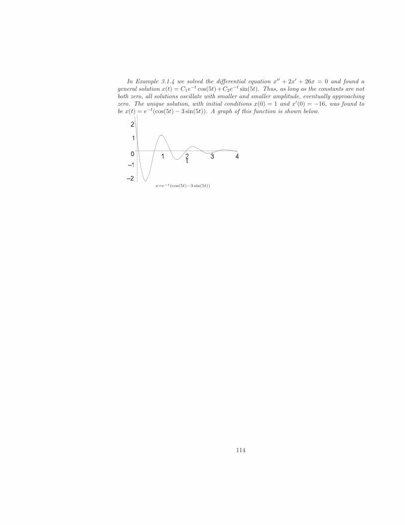
In Example 3.1.4 we solved the differential equation x′′ + 2x′ + 26x = 0 and found ageneral solution x(t) = C1e
−t cos(5t)+C2e−t sin(5t). Thus, as long as the constants are not
both zero, all solutions oscillate with smaller and smaller amplitude, eventually approachingzero. The unique solution, with initial conditions x(0) = 1 and x′(0) = −16, was found tobe x(t) = e−t(cos(5t)− 3 sin(5t)). A graph of this function is shown below.
= >= ?@ ?> ? > A BCx=e−t(cos(5t)−3 sin(5t))
114
Exercises 3.1 Determine whether each of the following equations is linear or nonlinear. Ifit is linear state whether it is homogeneous or not.
1. x′′ + t2x′ + sin(t)x = 0
2. x′′ + t2x′ + t sin(x) = 0
3. t2x′′ + tx′ + x+ t = 0
4. t2x′′ + tx′ + 3x = 0
5. x′′ + x2 = 0
6. x′′ + t2 = 0
For equations 7 and 8 below two functions x1 and x2 are given. Show that x1 and x2
are both solutions of the equation and that x1 and x2 linearly independent. then givethe general solution.
7. t2x′′ − 2tx′ + 2x = 0, t > 0, x1 = t, x2 = t2
8. t2y′′ + y = 0, t > 0, y1 =√t cos
(12 (ln t)
√3), y2 =
√t sin
(12 (ln t)
√3)
Find a general solution to each of the following
9. x′′ + 7x′ + 10x = 0
10. x′′ − 3x′ + x = 0
11. x′′ + 6x′ + 9x = 0
12. y′′ − y′ + 14y = 0
13. y′′ + 2y′ + 5y = 0
14. x′′ + x′ + x = 0
Find the solution to each of the following initial value problems, and describe thebehavior of each solution. Also, sketch a graph of each solution (choose an appropriateviewing window to illustrate the principles discussed in Example 3.1.5 ).
15. 2y′′ + 3y′ − 9y = 0, y(0) = 1, y′(0) = 0
16. y′′ + 0.3y′ + 0.02y = 0, x(0) = 2, x′(0) = −5
17. 4x′′ − 4x′ + x = 0, x(0) = 0, x′(0) = 1
18. y′′ − 2y′ + 5y = 0, y(0) = 1, y′(0) = 1
19. For each of the three values c = 0.22, 0.23, and 0.24, solve the initial-value problem
x′′ + cx′ + 0.013225x = 0, x(0) = 2, x′(0) = 0.
Explain what is happening as the value of c increases.
20. For the “one real root” case (i.e. when b2 − 4ac = 0), show that if erx is one solutionof ax′′ + bx′ + cx = 0, then xerx is also a solution. Hint: Substitute y = xerx into theequation and use the fact that r = − b
2a .
115
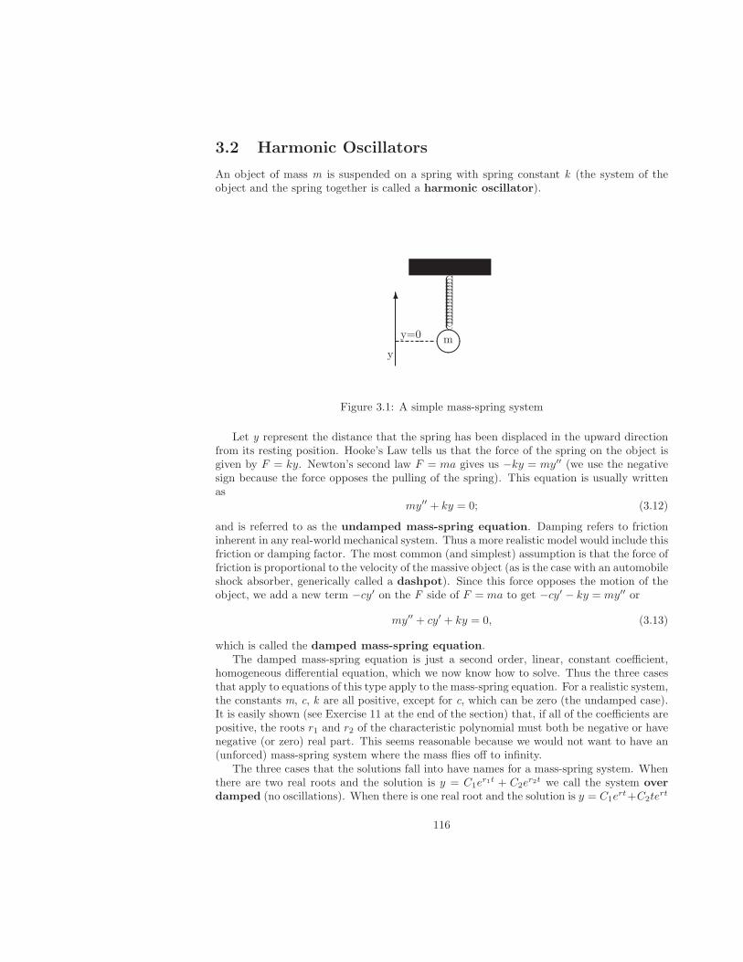
3.2 Harmonic Oscillators
An object of mass m is suspended on a spring with spring constant k (the system of theobject and the spring together is called a harmonic oscillator).
����
CCCCCCCCCCCCCCC
6
y=0 m
y
Figure 3.1: A simple mass-spring system
Let y represent the distance that the spring has been displaced in the upward directionfrom its resting position. Hooke’s Law tells us that the force of the spring on the object isgiven by F = ky. Newton’s second law F = ma gives us −ky = my′′ (we use the negativesign because the force opposes the pulling of the spring). This equation is usually writtenas
my′′ + ky = 0; (3.12)
and is referred to as the undamped mass-spring equation. Damping refers to frictioninherent in any real-world mechanical system. Thus a more realistic model would include thisfriction or damping factor. The most common (and simplest) assumption is that the force offriction is proportional to the velocity of the massive object (as is the case with an automobileshock absorber, generically called a dashpot). Since this force opposes the motion of theobject, we add a new term −cy′ on the F side of F = ma to get −cy′ − ky = my′′ or
my′′ + cy′ + ky = 0, (3.13)
which is called the damped mass-spring equation.The damped mass-spring equation is just a second order, linear, constant coefficient,
homogeneous differential equation, which we now know how to solve. Thus the three casesthat apply to equations of this type apply to the mass-spring equation. For a realistic system,the constants m, c, k are all positive, except for c, which can be zero (the undamped case).It is easily shown (see Exercise 11 at the end of the section) that, if all of the coefficients arepositive, the roots r1 and r2 of the characteristic polynomial must both be negative or havenegative (or zero) real part. This seems reasonable because we would not want to have an(unforced) mass-spring system where the mass flies off to infinity.
The three cases that the solutions fall into have names for a mass-spring system. Whenthere are two real roots and the solution is y = C1e
r1t + C2er2t we call the system over
damped (no oscillations). When there is one real root and the solution is y = C1ert+C2te
rt
116
we call the system critically damped (again no oscillations). When there are complexroots α±βi and the solution is y = C1e
αt cos(βt)+C2eαt sin(βt), we call the system under
damped (the system oscillates). Note that for a mass-spring equation the discriminantof the characteristic polynomial is c2 − 4mk, so that the system is under damped if thedamping constant c satisfies c <
√4mk (c small) and over damped if c >
√4mk (c large).
Note on frequency and period. The functions cos(ωt) and sin(ωt) each complete a fullcycle on the t-interval from 0 to 2π
ω and hence complete ω2π cycles on the interval from 0 to
1. We call 2πω the period and ω
2π the frequency. We can use these terms for functionssuch as eαt cos(βt) and eαt sin(βt) as well, in that they represent “periodic” functions withvariable amplitude (the zeroes of these functions are not affected by the eαt term).
Note on amplitude and phase shift. The trig identity cos(A − B) = cos(A) cos(B) +sin(A) sin(B) can be used to convert a function of the form C1 cos(βt) + C2 sin(βt) intoa single cosine function D cos(βt − φ). We call D the amplitude and φ the phase. Theformulas for converting from one form to the other are obtained by writing D cos(βt −φ) = D(cos(βt) cos(φ) + sin(βt) sin(φ)) = C1 cos(βt) + C2 sin(βt); then C1 = D cos(φ) andC2 = D sin(φ). Solving for D and φ we have D2 = C2
1 + C22 and tan(φ) = C2/C1, subject
to the condition C1 = D cos(φ) (use either φ = arctan(C2/C1) or φ = arctan(C2/C1) + π,whichever satisfies C1 = D cos(φ)). The function cos(βt− φ) is shifted φ
β units to the right
of cos(βt), or φ2π cycles to the right of cos(βt). Notice also that by factoring out the eαt
term in the under damped case (complex roots) we get
C1eαt cos(βt) + C2e
αt sin(βt) =
eαt(C1 cos(βt) + C2 sin(βt)) = Deαt cos(βt− φ).
Similarly, if we want to write the result as a single sine function D sin(βt − φ) instead ofa single cosine function, the trig identity sin(A − B) = sin(A) cos(B) − cos(A) sin(B) canbe used to show that the corresponding formulas are D2 = C2
1 + C22 and tan(φ) = −C1/C2
subject to C2 = D cos(φ).
Note on units. This being a mathematics course, we will take the easy way out and alwaysuse the same units. We just need to know that a force of 1 Newton (n) will accelerate amass of 1 kilogram (kg) at a rate of 1 meter per second squared (s2) so that 1n = 1kg·m
s2 .The mass m will be in kilograms, the spring constant k will be in Newtons per meter
(nm
)
which is the same as kgs2 , and the damping constant c will be in Newtons per meter per
second(
nm/s = n·s
m
)
which is the same as kgs .
Example 3.2.1 A 1 kg mass is suspended on a spring with a spring constant of 16 nm . The
mass is displaced 0.5 meters in the positive y direction from its rest position and released.Assume no damping. Find the equation that describes the position (y) of the mass as afunction of time (t). Describe the motion.
The differential equation of motion for the position of the mass would be y′′ +16y = 0. Theinitial condition on the position would be y(0) = 0.5. The initial condition on the velocitywould be y′(0) = 0 because we assume that the mass is released with no initial velocity (it
117
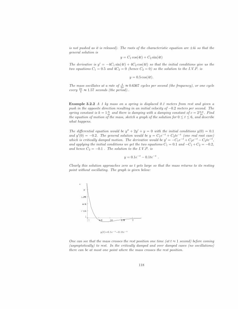
is not pushed as it is released). The roots of the characteristic equation are ±4i so that thegeneral solution is
y = C1 cos(4t) + C2 sin(4t)
The derivative is y′ = −4C1 sin(4t) + 4C2 cos(4t) so that the initial conditions give us thetwo equations C1 = 0.5 and 4C2 = 0 (hence C2 = 0) so the solution to the I.V.P. is
y = 0.5 cos(4t).
The mass oscillates at a rate of 42π ≈ 0.6367 cycles per second (the frequency), or one cycle
every 2π4 ≈ 1.57 seconds (the period)..
Example 3.2.2 A 1 kg mass on a spring is displaced 0.1 meters from rest and given apush in the opposite direction resulting in an initial velocity of −0.2 meters per second. Thespring constant is k = 1 n
m and there is damping with a damping constant of c = 2n·sm . Find
the equation of motion of the mass, sketch a graph of the solution for 0 ≤ t ≤ 6, and describewhat happens.
The differential equation would be y′′ + 2y′ + y = 0 with the initial conditions y(0) = 0.1and y′(0) = −0.2. The general solution would be y = C1e
−t + C2te−t (one real root case)
which is critically damped motion. The derivative would be y′ = −C1e−t +C2e
−t −C2te−t,
and applying the initial conditions we get the two equations C1 = 0.1 and −C1+C2 = −0.2,and hence C2 = −0.1 . The solution to the I.V.P. is
y = 0.1e−t − 0.1te−t .
Clearly this solution approaches zero as t gets large so that the mass returns to its restingpoint without oscillating. The graph is given below:
DE F G DH F DI F H DJJ F IJ F J G DJ F J DJ F J H D J K
LK
Ly(t)=0.1e−t−0.1te−t
One can see that the mass crosses the rest position one time (at t ≈ 1 second) before coming(asymptotically) to rest. In the critically damped and over damped cases (no oscillations)there can be at most one point where the mass crosses the rest position.
118
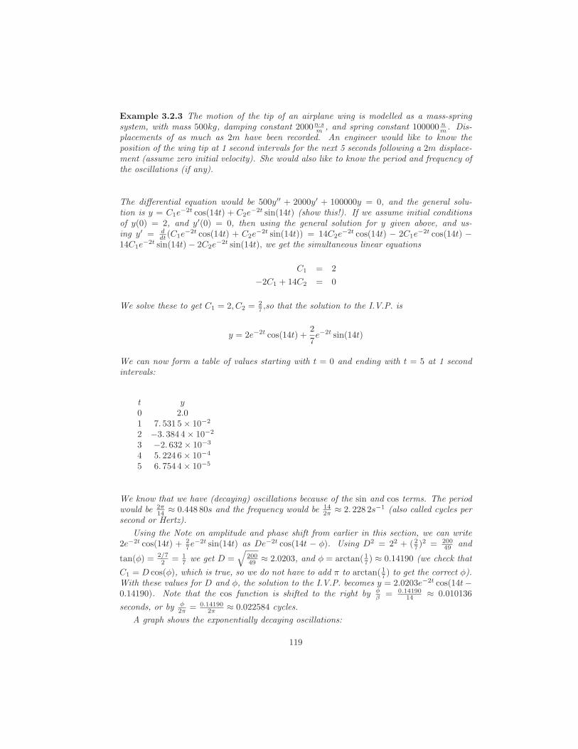
Example 3.2.3 The motion of the tip of an airplane wing is modelled as a mass-springsystem, with mass 500kg, damping constant 2000n·s
m , and spring constant 100000 nm . Dis-
placements of as much as 2m have been recorded. An engineer would like to know theposition of the wing tip at 1 second intervals for the next 5 seconds following a 2m displace-ment (assume zero initial velocity). She would also like to know the period and frequency ofthe oscillations (if any).
The differential equation would be 500y′′ + 2000y′ + 100000y = 0, and the general solu-tion is y = C1e
−2t cos(14t) + C2e−2t sin(14t) (show this!). If we assume initial conditions
of y(0) = 2, and y′(0) = 0, then using the general solution for y given above, and us-ing y′ = d
dt (C1e−2t cos(14t) + C2e
−2t sin(14t)) = 14C2e−2t cos(14t) − 2C1e
−2t cos(14t) −14C1e
−2t sin(14t)− 2C2e−2t sin(14t), we get the simultaneous linear equations
C1 = 2
−2C1 + 14C2 = 0
We solve these to get C1 = 2, C2 = 27 ,so that the solution to the I.V.P. is
y = 2e−2t cos(14t) +2
7e−2t sin(14t)
We can now form a table of values starting with t = 0 and ending with t = 5 at 1 secondintervals:
t y0 2.01 7. 531 5× 10⁻²
2 −3. 384 4× 10⁻²
3 −2. 632× 10−3
4 5. 224 6× 10⁻⁴
5 6. 754 4× 10⁻⁵
We know that we have (decaying) oscillations because of the sin and cos terms. The periodwould be 2π
14 ≈ 0.448 80s and the frequency would be 142π ≈ 2. 228 2s−1 (also called cycles per
second or Hertz).
Using the Note on amplitude and phase shift from earlier in this section, we can write2e−2t cos(14t) + 2
7e−2t sin(14t) as De−2t cos(14t − φ). Using D2 = 22 + ( 27 )
2 = 20049 and
tan(φ) = 2/72 = 1
7 we get D =√
20049 ≈ 2.0203, and φ = arctan( 17 ) ≈ 0.14190 (we check that
C1 = D cos(φ), which is true, so we do not have to add π to arctan( 17 ) to get the correct φ).With these values for D and φ, the solution to the I.V.P. becomes y = 2.0203e−2t cos(14t−0.14190). Note that the cos function is shifted to the right by φ
β = 0.1419014 ≈ 0.010136
seconds, or by φ2π = 0.14190
2π ≈ 0.022584 cycles.
A graph shows the exponentially decaying oscillations:
119
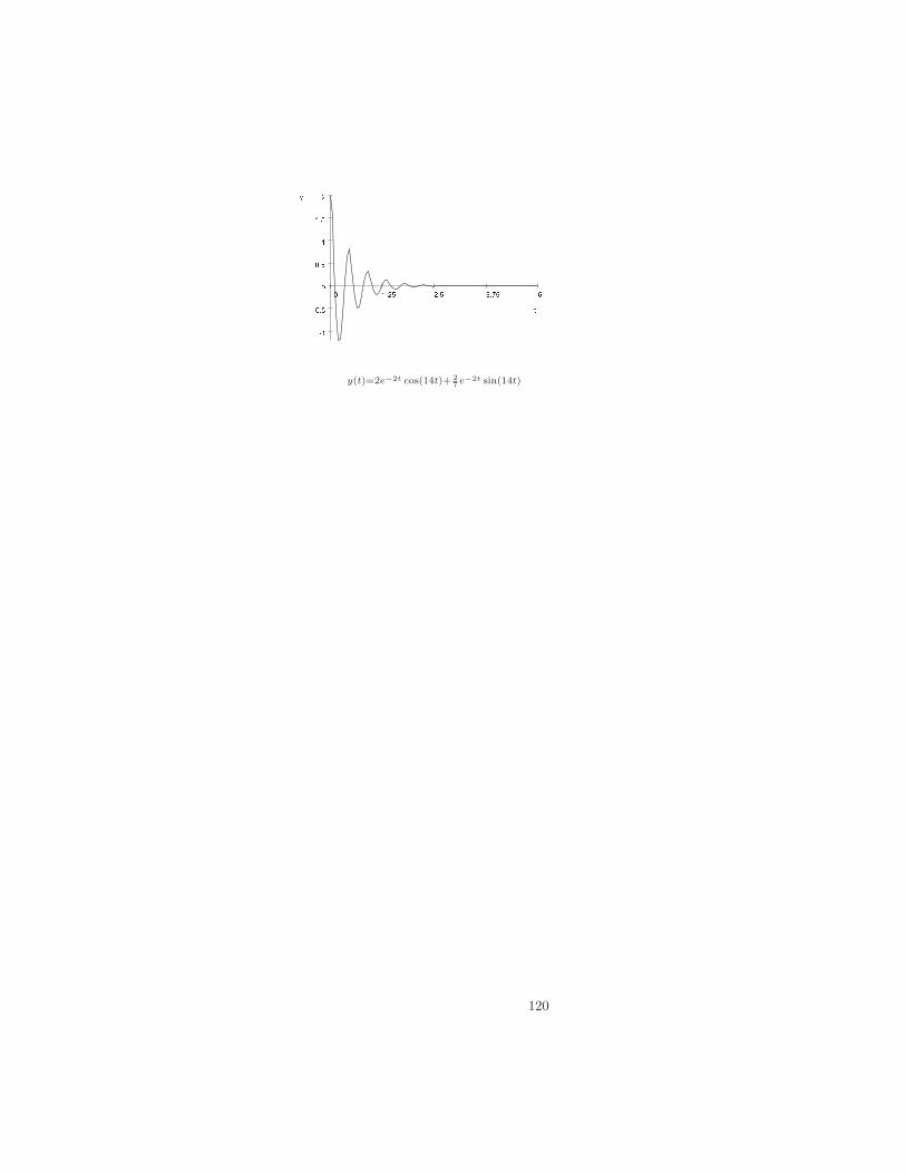
MN O P MQ O MR O Q MSQR O M RS O M ST S O MT R U
VU
Vy(t)=2e−2t cos(14t)+ 2
7e−2t sin(14t)
120
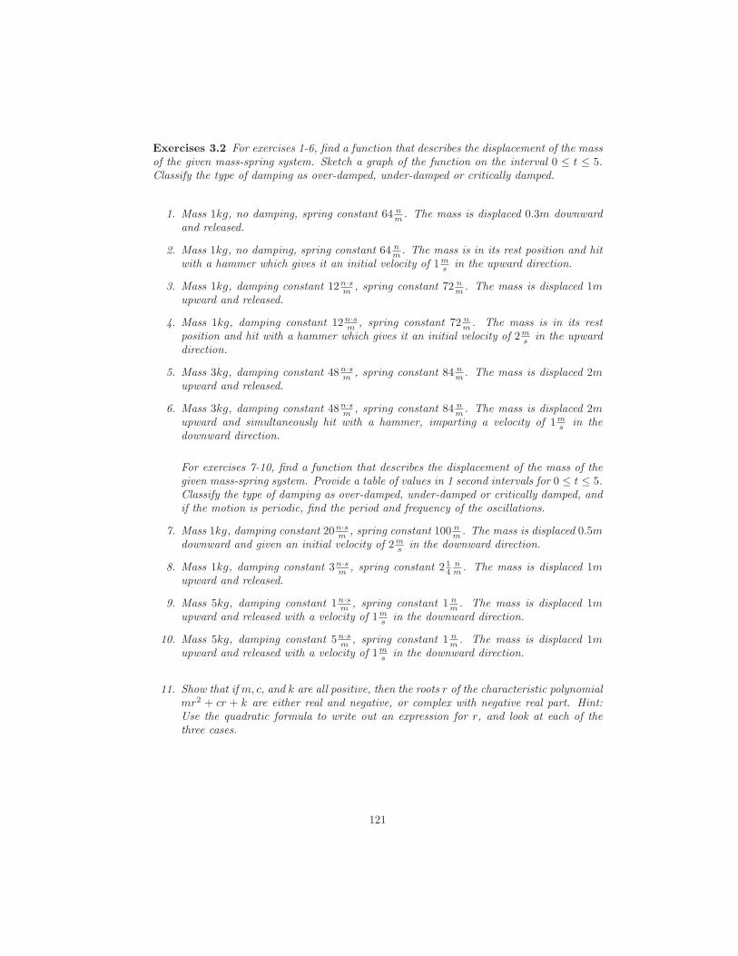
Exercises 3.2 For exercises 1-6, find a function that describes the displacement of the massof the given mass-spring system. Sketch a graph of the function on the interval 0 ≤ t ≤ 5.Classify the type of damping as over-damped, under-damped or critically damped.
1. Mass 1kg, no damping, spring constant 64 nm . The mass is displaced 0.3m downward
and released.
2. Mass 1kg, no damping, spring constant 64 nm . The mass is in its rest position and hit
with a hammer which gives it an initial velocity of 1ms in the upward direction.
3. Mass 1kg, damping constant 12n·sm , spring constant 72 n
m . The mass is displaced 1mupward and released.
4. Mass 1kg, damping constant 12n·sm , spring constant 72 n
m . The mass is in its restposition and hit with a hammer which gives it an initial velocity of 2m
s in the upwarddirection.
5. Mass 3kg, damping constant 48n·sm , spring constant 84 n
m . The mass is displaced 2mupward and released.
6. Mass 3kg, damping constant 48n·sm , spring constant 84 n
m . The mass is displaced 2mupward and simultaneously hit with a hammer, imparting a velocity of 1m
s in thedownward direction.
For exercises 7-10, find a function that describes the displacement of the mass of thegiven mass-spring system. Provide a table of values in 1 second intervals for 0 ≤ t ≤ 5.Classify the type of damping as over-damped, under-damped or critically damped, andif the motion is periodic, find the period and frequency of the oscillations.
7. Mass 1kg, damping constant 20n·sm , spring constant 100 n
m . The mass is displaced 0.5mdownward and given an initial velocity of 2m
s in the downward direction.
8. Mass 1kg, damping constant 3n·sm , spring constant 2 1
4nm . The mass is displaced 1m
upward and released.
9. Mass 5kg, damping constant 1n·sm , spring constant 1 n
m . The mass is displaced 1mupward and released with a velocity of 1m
s in the downward direction.
10. Mass 5kg, damping constant 5n·sm , spring constant 1 n
m . The mass is displaced 1mupward and released with a velocity of 1m
s in the downward direction.
11. Show that if m, c, and k are all positive, then the roots r of the characteristic polynomialmr2 + cr + k are either real and negative, or complex with negative real part. Hint:Use the quadratic formula to write out an expression for r, and look at each of thethree cases.
121
3.3 Nonhomogeneous Constant Coefficient Linear Dif-
ferential Equations
We now turn our attention to the nonhomogeneous case. We are interested in solvingequations of the form
ax′′ + bx′ + cx = f(t) (3.14)
where f(t) can consist of a linear combination of polynomials, exponential functions, andtrig functions (as described later in the section). Notice also that if f(t) depends explicitlyon t, such a differential equation is also nonautonomous.
The next theorem leads to a method for finding the general solution to Equation (3.14).
Theorem 3.4 If xh is the general solution of the homogeneous equation ax′′+ bx′+ cx = 0and xp is any solution of Equation (3.14), then the general solution to Equation (3.14) isthe sum x = xh + xp
The solution xp to Equation (3.14) is called a particular solution. Since we alreadyknow how to solve the homogeneous case (Section 3.1), we only need a technique for findinga particular solution of equation (3.14). In this section we will employ the method ofundetermined coefficients. This consists of proposing a solution xP which has arbitraryconstants in it (the undetermined coefficients), substituting the proposed solution xP intothe differential equation, and then solving for the arbitrary constants by equating coefficientsof like terms. Note the similarity to the method of Section 3.1 where we proposed a solutionx = ert to a homogeneous linear differential equation, and then solved for r.
The question that remains is how to determine the form of the proposed solution xP .The form of xP depends on the form of the function f(t) in equation (3.14). Basically xP
must have a form similar to that of f(t). We sometimes need a two step process; a firstattempt, step 1 below, and if that attempt fails, a second attempt, step 2 below.
122
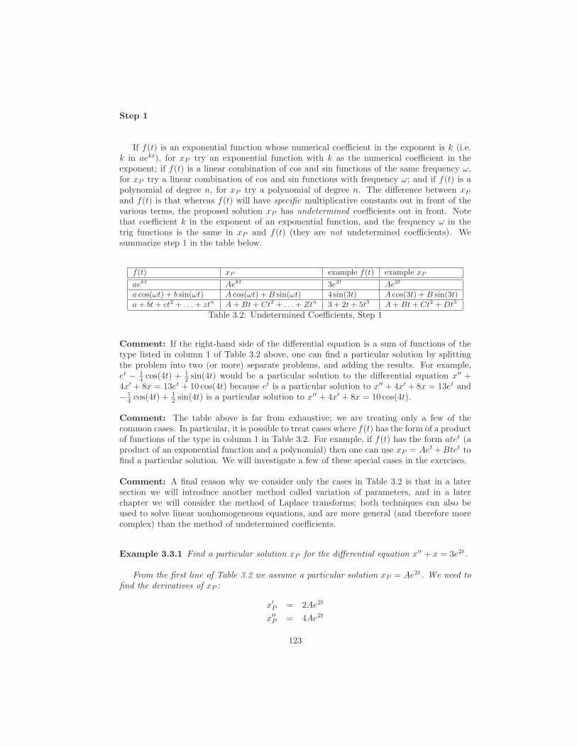
Step 1
If f(t) is an exponential function whose numerical coefficient in the exponent is k (i.e.k in aekt), for xP try an exponential function with k as the numerical coefficient in theexponent; if f(t) is a linear combination of cos and sin functions of the same frequency ω,for xP try a linear combination of cos and sin functions with frequency ω; and if f(t) is apolynomial of degree n, for xP try a polynomial of degree n. The difference between xP
and f(t) is that whereas f(t) will have specific multiplicative constants out in front of thevarious terms, the proposed solution xP has undetermined coefficients out in front. Notethat coefficient k in the exponent of an exponential function, and the frequency ω in thetrig functions is the same in xP and f(t) (they are not undetermined coefficients). Wesummarize step 1 in the table below.
f(t) xP example f(t) example xP
aekt Aekt 3e2t Ae2t
a cos(ωt) + b sin(ωt) A cos(ωt) +B sin(ωt) 4 sin(3t) A cos(3t) +B sin(3t)
a+ bt+ ct2 + . . .+ ztn A+Bt+ Ct2 + . . .+ Ztn 3 + 2t+ 5t3 A+Bt+ Ct2 +Dt3
Table 3.2: Undetermined Coefficients, Step 1
Comment: If the right-hand side of the differential equation is a sum of functions of thetype listed in column 1 of Table 3.2 above, one can find a particular solution by splittingthe problem into two (or more) separate problems, and adding the results. For example,et − 1
4 cos(4t) +12 sin(4t) would be a particular solution to the differential equation x′′ +
4x′ + 8x = 13et + 10 cos(4t) because et is a particular solution to x′′ + 4x′ + 8x = 13et and− 1
4 cos(4t) +12 sin(4t) is a particular solution to x′′ + 4x′ + 8x = 10 cos(4t).
Comment: The table above is far from exhaustive; we are treating only a few of thecommon cases. In particular, it is possible to treat cases where f(t) has the form of a productof functions of the type in column 1 in Table 3.2. For example, if f(t) has the form atet (aproduct of an exponential function and a polynomial) then one can use xP = Aet +Btet tofind a particular solution. We will investigate a few of these special cases in the exercises.
Comment: A final reason why we consider only the cases in Table 3.2 is that in a latersection we will introduce another method called variation of parameters, and in a laterchapter we will consider the method of Laplace transforms; both techniques can also beused to solve linear nonhomogeneous equations, and are more general (and therefore morecomplex) than the method of undetermined coefficients.
Example 3.3.1 Find a particular solution xP for the differential equation x′′ + x = 3e2t.
From the first line of Table 3.2 we assume a particular solution xP = Ae2t. We need tofind the derivatives of xP :
x′P = 2Ae2t
x′′P = 4Ae2t
123
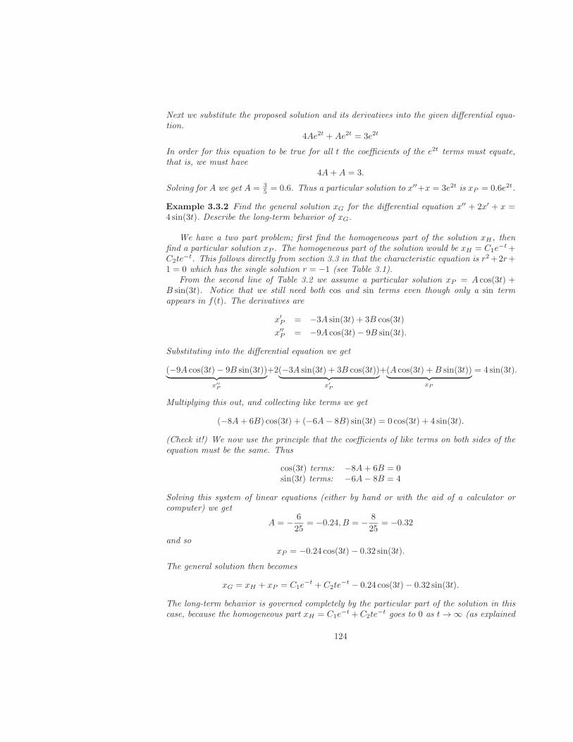
Next we substitute the proposed solution and its derivatives into the given differential equa-tion.
4Ae2t +Ae2t = 3e2t
In order for this equation to be true for all t the coefficients of the e2t terms must equate,that is, we must have
4A+A = 3.
Solving for A we get A = 35 = 0.6. Thus a particular solution to x′′+x = 3e2t is xP = 0.6e2t.
Example 3.3.2 Find the general solution xG for the differential equation x′′ + 2x′ + x =4 sin(3t). Describe the long-term behavior of xG.
We have a two part problem; first find the homogeneous part of the solution xH , thenfind a particular solution xP . The homogeneous part of the solution would be xH = C1e
−t+C2te
−t. This follows directly from section 3.3 in that the characteristic equation is r2+2r+1 = 0 which has the single solution r = −1 (see Table 3.1).
From the second line of Table 3.2 we assume a particular solution xP = A cos(3t) +B sin(3t). Notice that we still need both cos and sin terms even though only a sin termappears in f(t). The derivatives are
x′P = −3A sin(3t) + 3B cos(3t)
x′′P = −9A cos(3t)− 9B sin(3t).
Substituting into the differential equation we get
(−9A cos(3t)− 9B sin(3t))︸ ︷︷ ︸
x′′
P
+2(−3A sin(3t) + 3B cos(3t))︸ ︷︷ ︸
x′
P
+(A cos(3t) +B sin(3t))︸ ︷︷ ︸
xP
= 4 sin(3t).
Multiplying this out, and collecting like terms we get
(−8A+ 6B) cos(3t) + (−6A− 8B) sin(3t) = 0 cos(3t) + 4 sin(3t).
(Check it!) We now use the principle that the coefficients of like terms on both sides of theequation must be the same. Thus
cos(3t) terms: −8A+ 6B = 0sin(3t) terms: −6A− 8B = 4
Solving this system of linear equations (either by hand or with the aid of a calculator orcomputer) we get
A = − 6
25= −0.24, B = − 8
25= −0.32
and soxP = −0.24 cos(3t)− 0.32 sin(3t).
The general solution then becomes
xG = xH + xP = C1e−t + C2te
−t − 0.24 cos(3t)− 0.32 sin(3t).
The long-term behavior is governed completely by the particular part of the solution in thiscase, because the homogeneous part xH = C1e
−t +C2te−t goes to 0 as t → ∞ (as explained
124
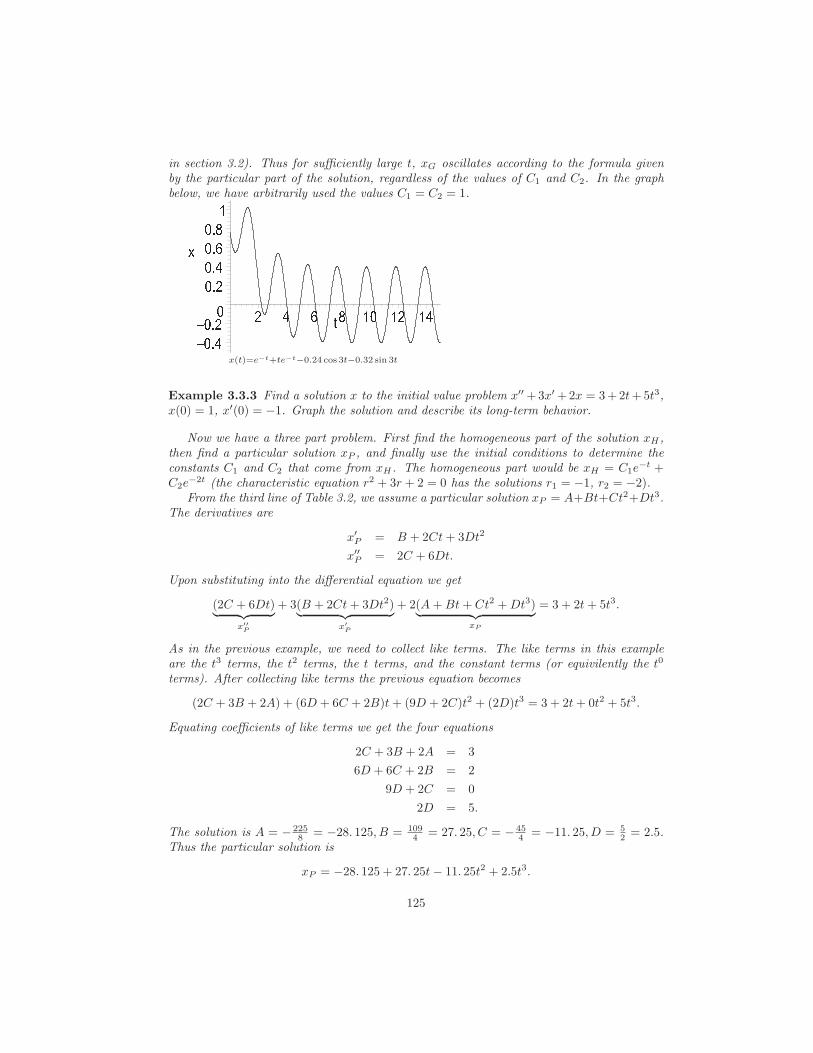
in section 3.2). Thus for sufficiently large t, xG oscillates according to the formula givenby the particular part of the solution, regardless of the values of C1 and C2. In the graphbelow, we have arbitrarily used the values C1 = C2 = 1.
W X Y ZW X Y [ XX Y [X Y ZX Y \X Y ] ^_ [ Z \ ] ^ X ^ [ ^ Z`x(t)=e−t+te−t−0.24 cos 3t−0.32 sin 3t
Example 3.3.3 Find a solution x to the initial value problem x′′ +3x′ +2x = 3+2t+5t3,x(0) = 1, x′(0) = −1. Graph the solution and describe its long-term behavior.
Now we have a three part problem. First find the homogeneous part of the solution xH ,then find a particular solution xP , and finally use the initial conditions to determine theconstants C1 and C2 that come from xH . The homogeneous part would be xH = C1e
−t +C2e
−2t (the characteristic equation r2 + 3r + 2 = 0 has the solutions r1 = −1, r2 = −2).From the third line of Table 3.2, we assume a particular solution xP = A+Bt+Ct2+Dt3.
The derivatives are
x′P = B + 2Ct+ 3Dt2
x′′P = 2C + 6Dt.
Upon substituting into the differential equation we get
(2C + 6Dt)︸ ︷︷ ︸
x′′
P
+ 3(B + 2Ct+ 3Dt2)︸ ︷︷ ︸
x′
P
+ 2(A+Bt+ Ct2 +Dt3)︸ ︷︷ ︸
xP
= 3 + 2t+ 5t3.
As in the previous example, we need to collect like terms. The like terms in this exampleare the t3 terms, the t2 terms, the t terms, and the constant terms (or equivilently the t0
terms). After collecting like terms the previous equation becomes
(2C + 3B + 2A) + (6D + 6C + 2B)t+ (9D + 2C)t2 + (2D)t3 = 3 + 2t+ 0t2 + 5t3.
Equating coefficients of like terms we get the four equations
2C + 3B + 2A = 3
6D + 6C + 2B = 2
9D + 2C = 0
2D = 5.
The solution is A = − 2258 = −28. 125, B = 109
4 = 27. 25, C = − 454 = −11. 25, D = 5
2 = 2.5.Thus the particular solution is
xP = −28. 125 + 27. 25t− 11. 25t2 + 2.5t3.
125
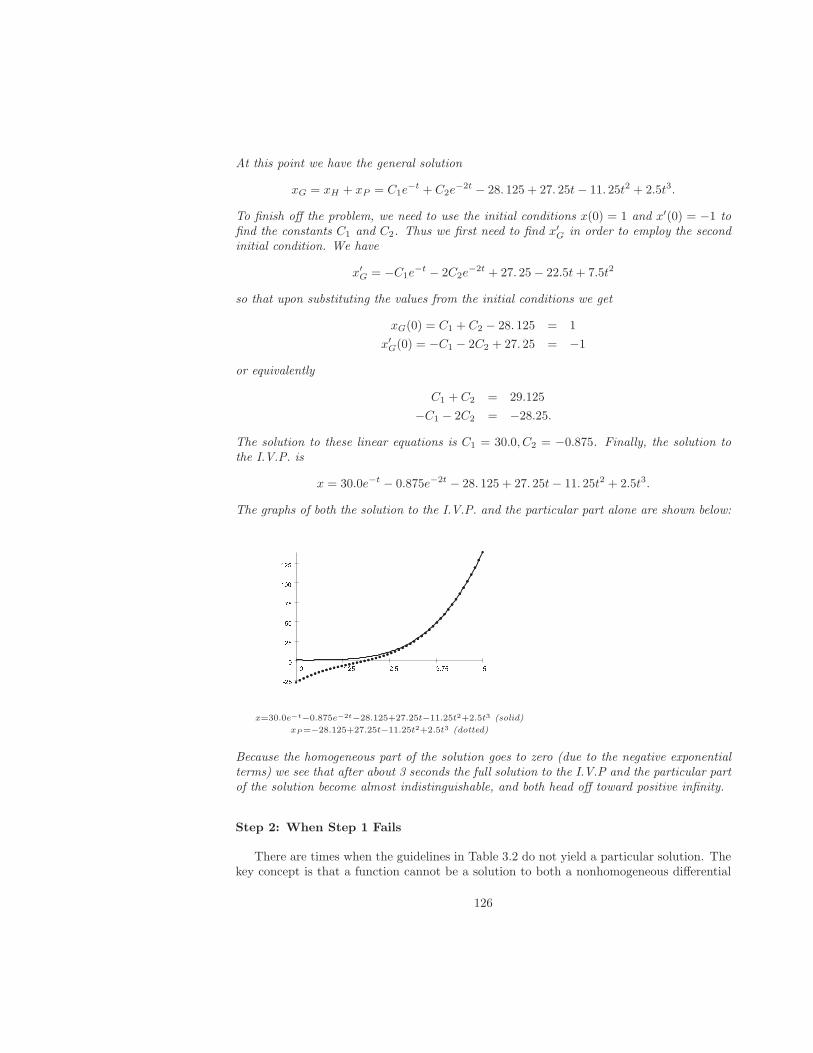
At this point we have the general solution
xG = xH + xP = C1e−t + C2e
−2t − 28. 125 + 27. 25t− 11. 25t2 + 2.5t3.
To finish off the problem, we need to use the initial conditions x(0) = 1 and x′(0) = −1 tofind the constants C1 and C2. Thus we first need to find x′
G in order to employ the secondinitial condition. We have
x′G = −C1e
−t − 2C2e−2t + 27. 25− 22.5t+ 7.5t2
so that upon substituting the values from the initial conditions we get
xG(0) = C1 + C2 − 28. 125 = 1
x′G(0) = −C1 − 2C2 + 27. 25 = −1
or equivalently
C1 + C2 = 29.125
−C1 − 2C2 = −28.25.
The solution to these linear equations is C1 = 30.0, C2 = −0.875. Finally, the solution tothe I.V.P. is
x = 30.0e−t − 0.875e−2t − 28. 125 + 27. 25t− 11. 25t2 + 2.5t3.
The graphs of both the solution to the I.V.P. and the particular part alone are shown below:
MN O P MQ O MR O Q MSR Q MR S SP MM SQ M ST Q M UU
x=30.0e−t−0.875e−2t−28.125+27.25t−11.25t2+2.5t3 (solid)
xP=−28.125+27.25t−11.25t2+2.5t3 (dotted)
Because the homogeneous part of the solution goes to zero (due to the negative exponentialterms) we see that after about 3 seconds the full solution to the I.V.P and the particular partof the solution become almost indistinguishable, and both head off toward positive infinity.
Step 2: When Step 1 Fails
There are times when the guidelines in Table 3.2 do not yield a particular solution. Thekey concept is that a function cannot be a solution to both a nonhomogeneous differential
126
equation and to the corresponding homogeneous equation. It’s easy to see why. Suppose thatg(t) solves both ax′′+bx′+cx = f(t) and ax′′+bx′+cx = 0; then ag′′(t)+bg′(t)+cg(t) = f(t)and also ag′′(t) + bg′(t) + cg(t) = 0 which is clearly impossible unless f(t) = 0. Thus thesuggested solutions in Table 3.2 will fail if they also solve the corresponding homogeneousequation.
You may be wondering what happens if you go ahead with the proposed xP from Table3.2 when it is also a solution to the homogeneous equation. You will find that it is impos-sible to solve the system of linear equations that gives you the values of the undeterminedcoefficients. If you are using a calulator or computer to solve the linear system, you mayget an error message, and if you are solving the system by hand, you will come across acontradictory equation such as 0 = 1.
The way out of the dilemna is as follows:
When the proposed xP from Table 3.2 fails, multiply that xP by t and tryagain. Repeat if necessary.
Example 3.3.4 Find a particular solution to the differential equation x′′ − x = 4et.
We first try Step 1, in which the proposed xP would be xP = Aet. The derivativeswould be x′
P = Aet and x′′P = Aet and so substituting into the differential equation we get
Aet − Aet = 4et. This simplifies to 0 = 4et which is clearly impossible. We could haveseen this coming if we had looked at the homogeneous solution xH first; the characteristicequation is r2 − 1 = 0, which has the solutions r = ±1, so that xH = C1e
t + C2e−t. The
right-hand side of the differential equation f(t) = 4et matches xH for the case C1 = 4,C2 = 0 and hence is a solution to the homogeneous equation.
Thus we go to Step 2 and multiply our first try Aet by t to get
xP = Atet.
The derivatives are
x′P = Aet +Atet
x′′P = Aet +Aet +Atet = 2Aet +Atet
and substituting into the given differential equation we get
(2Aet +Atet)︸ ︷︷ ︸
x′′
P
− (Atet)︸ ︷︷ ︸
xP
= 4et.
Since the Atet terms cancel out we are left with 2Aet = 4et. Equating the coefficients of liketerms we get 2A = 4 or A = 2. Thus a particular solution is
xP = 2tet.
Example 3.3.5 Find the general solution to x′′ + 4x = 5 cos(2t). Sketch a graph of theparticular solution and discuss its significance.
This time we start with the homogeneous solution; we get xH = C1 cos(2t) + C2 sin(2t)because the solutions to the characteristic equation r2 + 4 = 0 are r = 0 ± 2i. At this
127
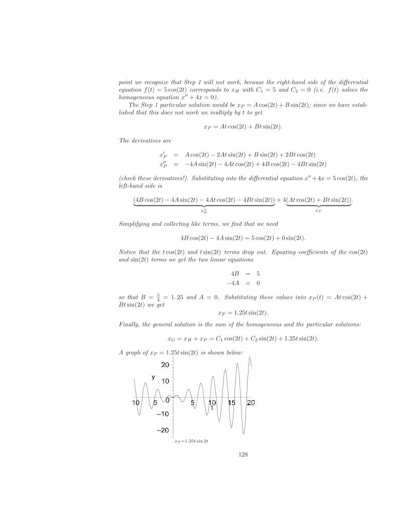
point we recognize that Step 1 will not work, because the right-hand side of the differentialequation f(t) = 5 cos(2t) corresponds to xH with C1 = 5 and C2 = 0 (i.e. f(t) solves thehomogeneous equation x′′ + 4x = 0).
The Step 1 particular solution would be xP = A cos(2t) +B sin(2t); since we have estab-lished that this does not work we multiply by t to get
xP = At cos(2t) +Bt sin(2t).
The derivatives are
x′P = A cos(2t)− 2At sin(2t) +B sin(2t) + 2Bt cos(2t)
x′′P = −4A sin(2t)− 4At cos(2t) + 4B cos(2t)− 4Bt sin(2t)
(check these derivatives!). Substituting into the differential equation x′′+4x = 5 cos(2t), theleft-hand side is
(4B cos(2t)− 4A sin(2t)− 4At cos(2t)− 4Bt sin(2t))︸ ︷︷ ︸
x′′
P
+ 4(At cos(2t) +Bt sin(2t))︸ ︷︷ ︸
xP
.
Simplifying and collecting like terms, we find that we need
4B cos(2t)− 4A sin(2t) = 5 cos(2t) + 0 sin(2t).
Notice that the t cos(2t) and t sin(2t) terms drop out. Equating coefficients of the cos(2t)and sin(2t) terms we get the two linear equations
4B = 5
−4A = 0
so that B = 54 = 1. 25 and A = 0. Substituting these values into xP (t) = At cos(2t) +
Bt sin(2t) we get
xP = 1.25t sin(2t).
Finally, the general solution is the sum of the homogeneous and the particular solutions:
xG = xH + xP = C1 cos(2t) + C2 sin(2t) + 1.25t sin(2t).
A graph of xP = 1.25t sin(2t) is shown below:
a b ca d c cd cb cea d c a f f d c d f b cgxP=1.25t sin 2t
128
We view the function 1.25t sin(2t) as a sin function with frequency 22π = 1
π and withvariable amplitude 1.25t. Thus as t → ∞, xP does not approach a limit, but rather oscillateswith greater and greater amplitude. Since the homogeneous part of the solution C1 cos(2t)+C2 sin(2t) oscillates with constant amplitude, it has a diminishing affect on the generalsolution C1 cos(2t) + C2 sin(2t) + 1.25t sin(2t) and so the general solution looks nearly thesame as the particular solution for large t.
Exercises 3.3
1. Find a particular solution to y′′ − y = 4 cos(2t).
2. Find a particular solution to y′′ + 4y′ + 8y = 3e2t.
3. Find a particular solution to y′′ + y = 4 cos(t).
4. Find a particular solution to y′′ + 4y′ + 4y = 4e−2t. Hint: The “repeat if necessary”part of Step 2 applies here.
5. Find the general solution to y′′ − 2y′ + y = 2t.
6. Find the general solution to y′′ + 5y′ + 6y = 2e4t.
7. Find the general solution to y′′ − 3y′ + 2y = et.
8. Find the general solution to y′′ + 16y = sin(3t).
9. Find the solution to the I.V.P. y′′ + 2y′ + 2y = 2 cos(t), y(0) = 1, y′(0) = −1 .
10. Find the solution to the I.V.P. y′′ + y = − sin(t), y(0) = 0, y′(0) = 0 .
The following exercises require the use of the first comment following Table 3.2.
11. Find a particular solution to y′′ + 10y′ + 21y = et + t2.
12. Find a particular solution to y′′ + 9y = sin(t)− e2t.
13. Find the solution to the I.V.P. y′′ − 9y = t− cos(t), y(0) = 0, y′(0) = 1 .
14. Find the solution to the I.V.P. y′′ + 2y′ + y = sin(t) + cos(2t), y(0) = 0, y′(0) = 0 .
We elaborate on the second comment following Table 3.2. When the function f(t)on the right-hand side of a second order linear differential equation is a product offunctions of the type in the first column of Table 3.2, you can still use undeterminedcoefficients by assuming a product of the functions in the second column for yP . Pro-ceed as follows: set each undetermined coefficient in column 2 equal to 1, multiplyout the terms, and then put one new undetermined coefficient in front of each term.For example, f(t) = 3t sin(2t) is a product of a polynomial of degree one (column 1,row 3) and a sin function with ω = 2 (column 1, row 2). Thus assume a product ofa general polynomial of degree one A + Bt (column 2, row 3) and a linear combina-tion of sin and cos functions with ω = 2, A cos(2t) + B sin(2t) (column 2, row 2).Now set each coefficient equal to 1 and multiply out to get (1 + t)(cos(2t) + sin(2t)) =
129
cos(2t) + sin(2t) + t cos(2t) + t sin(2t); then put one new undetermined coefficient infront of each term, resulting in yP = A cos(2t) + B sin(2t) + Ct cos(2t) + Dt sin(2t).Use these ideas in the following exercises.
15. Find a particular solution to y′′ + y = 3t sin(2t).
16. Find a particular solution to y′′ + y = e−t cos(t).
17. Find the solution to the I.V.P. y′′ + 2y′ + y = tet, y(0) = 1, y′(0) = 0 .
18. Find the solution to the I.V.P. y′′ + 2y′ + 2y = e−t sin(t), y(0) = 0, y′(0) = 0 .
130
3.4 Driven Mass-Spring Systems, Beats, and Resonance
Consider a damped mass-spring system as described in Section 3.2, but with a new twist.Our systems will now have an external driving force. If you have ever observed a washingmachine wobbling as it spins (often due to an unbalanced arrangement of clothes inside themachine) then you have experienced a periodic driving force. A simplified model of the samephenomenon would be an airplane engine with a broken propeller. Such an engine, whenplaced on an airplane wing would cause the wing to vibrate up and down. The rotationalmotion of the propeller is transformed into a sinusoidal driving force. In fact, since noreal propeller system can be perfectly balanced, this is something that (propeller) airplanedesigners must consider.
Recall from Section 3.2 that by using Newton’s second law F = ma we derived thesecond order differential equation my′′ = −cy′ − ky where the right-hand side representsthe sum of all forces acting on a mass suspended from a spring, with −ky corresponding tothe force of the spring from Hooke’s Law and −cy′ corresponding to the damping (friction)force. If we now introduce a driving force f(t) as explained above, the equation becomesmy′′ = −cy′ − ky + f(t) or equivalently
my′′ + cy′ + ky = f(t). (3.15)
We refer to equation 3.15 as the driven mass-spring equation.By an incredible coincidence, equation 3.15 is a non-homogeneous, constant coefficient,
linear, second-order differential equation; just the type we studied in the previous section.Since we already know how to solve such equations, in this section we concentrate on theinterpretation of the solution to such an equation in terms of driven mass-spring systems.The point of view that we will take is that f(t) is the input to the system, and the solutionto the differential equation y(t) is the response or output.
We can now translate between the language of second order, linear, constant coefficientdifferential equations and the language of forced mass-spring systems. In particular, whensolving non-homogeneous second order equations we found that the general solution wasa sum of two pieces: the homogeneous piece yH and the particular piece yP . For forcedmass-spring systems, we will call the homogeneous part of the solution the transient partof the response (at least when damping is present), and we will call the particular part thesteady-state part of the solution. The next example should help to make sense out of theseterms.
Example 3.4.1 A 2 kg mass is suspended from a spring with spring constant 30 nm and
damping constant 16n·sm . It is neither displaced nor given an initial velocity. Find the
response (output) of the system if the input is a sinusoidal driving force with amplitude 400newtons and frequency of 6
π ≈ 1. 909 9 cycles per second (beginning its cycle at t = 0). Graphthe response function and relate the behavior to the input forcing function.
We have m = 2 for the mass, c = 16 for the damping constant, and k = 30 for the springconstant. A sin function with amplitude 400 and frequency 6
π = 122π cycles per second, and
beginning its cycle at t = 0, would be f(t) = 400 sin(12t) (recall from the Note on frequencyand period from Section 3.2 that the frequency of sin(ωt) is ω
2π ). Thus the differentialequation that we want to solve, using Equation 3.15, would be
2y′′ + 16y′ + 30y = 400 sin(12t).
131
Because the mass is neither displaced nor given an initial push, we have y(0) = 0 andy′(0) = 0 giving us an initial value problem (I.V.P.).
We need to find the homogeneous part of the solution yH , and then a particular solutionyP , and then add them together to find the general solution yG. The final step will be to usethe initial conditions to evaluate the arbitrary constants C1 and C2.
To find yH we need to solve the homogeneous differential equation 2y′′ +16y′ +30y = 0.The characteristic polynomial is 2r2 + 16r + 30, which has the roots r = −5, r = −3. Thuswe get
yH = C1e−5t + C2e
−3t.
To find yP we use undetermined coefficients as described in Section 3.3. We assume
yP = A cos(12t) +B sin(12t).
The derivatives are y′P = −12A sin(12t)+12B cos(12t), and y′′P = −144A cos(12t)−144B sin(12t).Substituting these into the nonhomogeneous differential equation above we get
2(−144A cos(12t)− 144B sin(12t)) + 16(−12A sin(12t) + 12B cos(12t))+30(A cos(12t) +B sin(12t)) = 400 sin(12t)
which upon combining like terms gives us
−258A cos(12t) + 192B cos(12t)− 192A sin(12t)− 258B sin(12t) = 400 sin(12t)
Equating the coefficients of the cos terms we get
−258A+ 192B = 0
(since there are no cos terms on the right-hand side), and equating the sin terms we get
−192A− 258B = 400.
Solving these last two equations for A and B results in
A = −6400
8619≈ −0.742 55, B = −8600
8619≈ −0.997 80
so that our particular solution is
yP = −0.742 55 cos(12t)− 0.997 80 sin(12t)
accurate to 5 digits. Thus the general solution is
yG = yH + yP = C1e−5t + C2e
−3t − 0.742 55 cos(12t)− 0.997 80 sin(12t).
To apply the initial conditions we need y′G :
y′G = −5C1e−5t − 3C2e
−3t + 8. 910 6 sin(12t)− 11. 974 cos(12t).
Using y(0) = 0 and y′(0) = 0 gives us the equations
C1 + C2 − 0.742 55 = 0−5C1 − 3C2 − 11. 974 = 0
132
which can be solved simultaneously for C1 and C2: C1 = −7. 100 8, C2 = 7. 843 4. Thereforethe solution to the I.V.P. is
y = −7. 100 8e−5t + 7. 843 4e−3t − 0.742 55 cos(12t)− 0.997 80 sin(12t).
A graph of this function is shown below:
MN O P MQ O MR O Q MSQ O M QR O M RS O M ST S O MT R U
VU
Vy=−7.100 8e−5t+7.8434e−3t−0.74255 cos(12t)−0.99780 sin(12t)
After roughly t = 2 we see that the graph has “settled down” into a steady state, a simplesinusoidal oscillation corresponding to the particluar or steady state part of the responseyP = −0.742 55 cos(12t) − 0.997 80 sin(12t). This is because the homogeneous or transientpart of the response yH = −7. 100 8e−5t+7. 843 4e−3t dies out due to the negative exponentialterms. The long-term behavior of yP mirrors the driving force f(t) = 400 sin(12t), in thatboth oscillate with a frequency of 6
π cycles per second.Using the Note on amplitude and phase shift from Section 3.2 we can write the steady
state part of the solution yP in the form D sin(12t−φ), which makes it easier to compare theinput to the output. We have D2 = 0.742 552 +0.997 802 = 1. 547 0 so that D =
√1. 547 0 =
1. 243 8. For φ we first try tan−1(−0.742 55/0.997 80) = −0.639 77, but this value does notwork for φ in the equation −0.997 80 = 1. 243 8 cos(φ) (the sign is wrong - check it) and sowe use φ = −0.639 77 + π = 2. 501 8. Thus we can write yP = 1. 243 8 sin(12t − 2. 501 8),which means that the steady-state response is shifted 2. 501 8
2π = 0.398 17 cycles to the right ofthe driving force. We could say that in the long-term, the response lags behind the drivingforce by about 0.4 cycles. We plot the driving force and the steady-state part of the response,one above the other, to illustrate this lag:
hi j k l mi j l mi j n o mi j mi j p l mi j o mi j h o mio m i iq o m i rs rs133
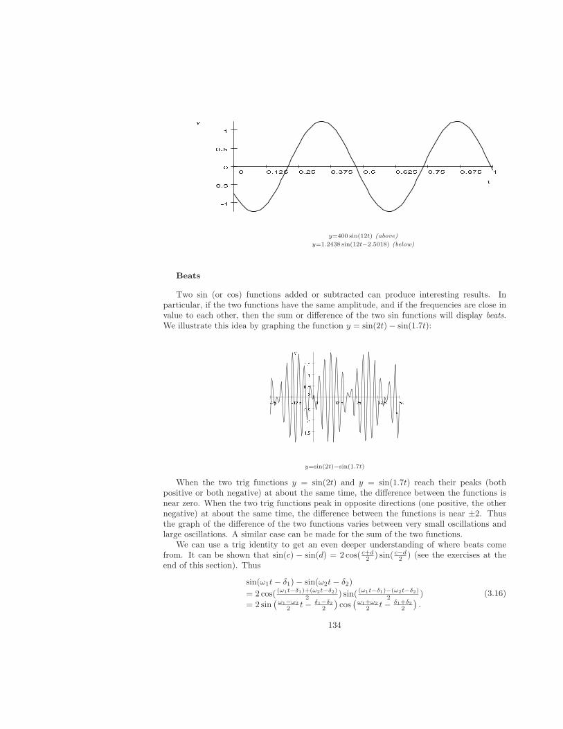
hi j k l mi j l mi j n o mi j mi j p l mi j o mi j h o mihi j m iq i j mq h rs rsy=400 sin(12t) (above)
y=1.2438 sin(12t−2.5018) (below)
Beats
Two sin (or cos) functions added or subtracted can produce interesting results. Inparticular, if the two functions have the same amplitude, and if the frequencies are close invalue to each other, then the sum or difference of the two sin functions will display beats.We illustrate this idea by graphing the function y = sin(2t)− sin(1.7t):
M SN P O MQ MR Q O MST R Q O MT Q M R O M RS O M ST S O MT RT R O M tV
tV
y=sin(2t)−sin(1.7t)
When the two trig functions y = sin(2t) and y = sin(1.7t) reach their peaks (bothpositive or both negative) at about the same time, the difference between the functions isnear zero. When the two trig functions peak in opposite directions (one positive, the othernegative) at about the same time, the difference between the functions is near ±2. Thusthe graph of the difference of the two functions varies between very small oscillations andlarge oscillations. A similar case can be made for the sum of the two functions.
We can use a trig identity to get an even deeper understanding of where beats comefrom. It can be shown that sin(c) − sin(d) = 2 cos( c+d
2 ) sin( c−d2 ) (see the exercises at the
end of this section). Thus
sin(ω1t− δ1)− sin(ω2t− δ2)
= 2 cos( (ω1t−δ1)+(ω2t−δ2)2 ) sin( (ω1t−δ1)−(ω2t−δ2)
2 )
= 2 sin(ω1−ω2
2 t− δ1−δ22
)cos
(ω1+ω2
2 t− δ1+δ22
).
(3.16)
134
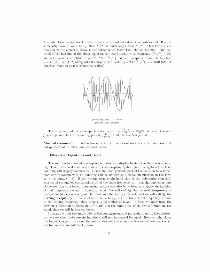
A similar formula applies if the sin functions are added rather than subtracted. If ω1 issufficently close in value to ω2, then
ω1+ω2
2 is much larger than ω1−ω2
2 . Therefore the cosfunction in the equation above is oscillating much faster than the sin function. One canthink of the last line of the above equation as a cos function with frequency
(ω1+ω2
2
)/ (2π)
and with variable amplitude 2 sin(ω1−ω2
2 t− δ1−δ22
). We can graph our example function
y = sin(2t)− sin(1.7t) along with its amplitude function y = 2 sin( 2−1.72 t) = 2 sin(0.15t) (or
envelope function as it is sometimes called):
M SN P O MQ MR Q O MST R Q O MT Q M QRST RT Q UV UVy=sin(2t)−sin(1.7t) (solid)
y=2 sin(0.15t) (dotted)
The frequency of the envelope function, given byω1−ω2
2
2π = ω1−ω2
4π , is called the beatfrequency, and the corresponding period, 4π
ω1−ω2, would be the beat period.
Musical comment: When two musical intruments sustain notes which are close, butnot quite equal, in pitch, one can hear beats.
Differential Equations and Beats
The solution to a forced mass-spring equation can display beats when there is no damp-ing. From Section 3.2 we saw that a free mass-spring system (no driving force) with nodamping will display oscillations. Hence the homogeneous part of the solution to a forcedmass-spring system with no damping can be written as a single sin function in the formyh = Ah sin(ωht − δ). If the driving term (right-hand side of the differential equation)consists of sin and/or cos functions all of the same frequency ωp, then the particular partof the solution to a forced mass-spring system can also be written as a single sin functionof that frequency, say yp = Ap sin(ωpt − φ). We will call ωh
2π the natural frequency ofthe system (it depends only on the mass and the spring constant) and we will call
ωp
2π thedriving frequency. If ωh is close in value to ωp, (i.e. if the natural frequency is closeto the driving frequency) then there is a possibility of beats. In fact, we know from theprevious subsection on beats that if in addition the amplitudes of the two sin functions areequal, then we will in fact see beats.
It turns out that the amplitudes of the homogeneous and particular parts of the solution,in the case when both are sin functions, will not in general be equal. However, the closerthe frequencies get, the closer the amplitudes get, and so in practice we will see beats whenthe frequencies are sufficiently close.
135
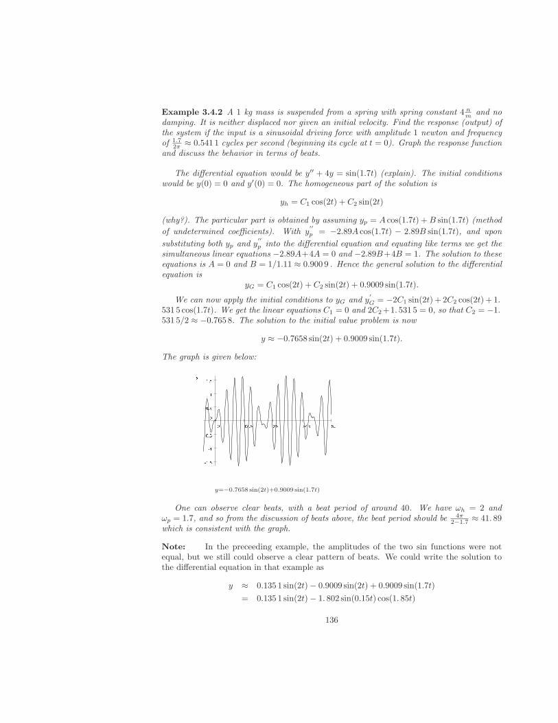
Example 3.4.2 A 1 kg mass is suspended from a spring with spring constant 4 nm and no
damping. It is neither displaced nor given an initial velocity. Find the response (output) ofthe system if the input is a sinusoidal driving force with amplitude 1 newton and frequencyof 1.7
2π ≈ 0.541 1 cycles per second (beginning its cycle at t = 0). Graph the response functionand discuss the behavior in terms of beats.
The differential equation would be y′′ + 4y = sin(1.7t) (explain). The initial conditionswould be y(0) = 0 and y′(0) = 0. The homogeneous part of the solution is
yh = C1 cos(2t) + C2 sin(2t)
(why?). The particular part is obtained by assuming yp = A cos(1.7t) +B sin(1.7t) (method
of undetermined coefficients). With y′′
p = −2.89A cos(1.7t) − 2.89B sin(1.7t), and upon
substituting both yp and y′′
p into the differential equation and equating like terms we get thesimultaneous linear equations −2.89A+4A = 0 and −2.89B+4B = 1. The solution to theseequations is A = 0 and B = 1/1.11 ≈ 0.900 9 . Hence the general solution to the differentialequation is
yG = C1 cos(2t) + C2 sin(2t) + 0.9009 sin(1.7t).
We can now apply the initial conditions to yG and y′
G = −2C1 sin(2t) + 2C2 cos(2t) + 1.531 5 cos(1.7t). We get the linear equations C1 = 0 and 2C2+1. 531 5 = 0, so that C2 = −1.531 5/2 ≈ −0.765 8. The solution to the initial value problem is now
y ≈ −0.7658 sin(2t) + 0.9009 sin(1.7t).
The graph is given below:
M SN P O MQ MR Q O MSR O M RS O M ST S O MT RT R O M UV UVy=−0.7658 sin(2t)+0.9009 sin(1.7t)
One can observe clear beats, with a beat period of around 40. We have ωh = 2 andωp = 1.7, and so from the discussion of beats above, the beat period should be 4π
2−1.7 ≈ 41. 89which is consistent with the graph.
Note: In the preceeding example, the amplitudes of the two sin functions were notequal, but we still could observe a clear pattern of beats. We could write the solution tothe differential equation in that example as
y ≈ 0.135 1 sin(2t)− 0.9009 sin(2t) + 0.9009 sin(1.7t)
= 0.135 1 sin(2t)− 1. 802 sin(0.15t) cos(1. 85t)
136
using the trig identities from the beat section above. The second term is the “beat” term; werefer to the first term as the “noise” term. The noise term is small in amplitude comparedto the beat term; if the noise term were too large, the beat pattern would be destroyed.
Resonance
We have seen that beats occur in differential equations when the natural and drivingfrequencies are close but not equal in value. What happens when the two frequencies areexactly equal? In this case we get the phenomenon called resonance. Since the beat periodis given by 4π
ωh−ωp, we see that as the driving frequency approaches the natural frequency,
the beat period goes to infinity, that is, the beats get longer and longer. It is also true thatthe beat amplitude gets larger as the two frequencies get close. Thus we can imagine thatas the driving frequency approaches the natural frequency, the beats get longer and larger,until we see an “infinitely long” beat, which continues to rise forever. This is called pureresonance.Note: Resonance can also be defined for a system in which there is a “small” amountof damping. It occurs when the frequency of a periodic forcing function is such that theresponse function attains a maximum amplitude. This will be covered in Chapter 6.
Example 3.4.3 A mass-spring system consists of a 1 kg mass suspended from a spring withspring constant 4 n
m . It is driven by a sinusoidal driving force with amplitude 1 newton andfrequency of 2
2π = 0.318 3 cycles per second (beginning its cycle at t = 0). Find the responseof the system, if there is no initial diplacement or initial velocity given. Sketch a graph ofthe response. Discuss the implications of your results.
The differential equation would be y′′ + 4y = sin(2t). The initial conditions would bey(0) = 0 and y′(0) = 0. The homogeneous part of the solution is
yh = C1 cos(2t) + C2 sin(2t).
A first attempt at a particular solution might be yp = A cos(2t) + B sin(2t). This attempt,however, quickly leads to a contradiction (show this) because yp solves the homogeneousdifferential equation y′′ + 4y = 0 (notice that the assumed form for yp is identical to yh).Thus we must go to Step 2 from Section 3.3, where we multiply the first guess by t. Thuswe now assume
yp = At cos(2t) +Bt sin(2t).
The derivatives are
y′p = A cos(2t)− 2At sin(2t) +B sin(2t) + 2Bt cos(2t)
y′′p = −4A sin(2t)− 4At cos(2t) + 4B cos(2t)− 4B sin(2t).
Substituting these into the differential equation we get
−4A sin(2t)− 4At cos(2t) + 4B cos(2t)− 4Bt sin(2t)︸ ︷︷ ︸
y′′
p
+ 4(At cos(2t) +Bt sin(2t))︸ ︷︷ ︸
yp
= sin(2t).
The terms that contain t cos(2t) and t sin(2t) cancel out, and so we only need equate coeffi-cients of the cos(2t) and sin(2t) terms. We get the linear equations
4B = 0
−4A = 1
137
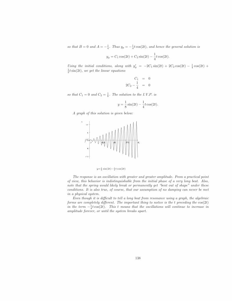
so that B = 0 and A = − 14 . Thus yp = − 1
4 t cos(2t), and hence the general solution is
yg = C1 cos(2t) + C2 sin(2t)−1
4t cos(2t).
Using the initial conditions, along with y′g = −2C1 sin(2t) + 2C2 cos(2t) − 14 cos(2t) +
12 t sin(2t), we get the linear equations
C1 = 0
2C2 −1
4= 0
so that C1 = 0 and C2 = 18 . The solution to the I.V.P. is
y =1
8sin(2t)− 1
4t cos(2t).
A graph of this solution is given below:
M SN P O MQ MR Q O MSR S MST MT R S UV
UV
y= 18sin(2t)− 1
4t cos(2t)
The response is an oscillation with greater and greater amplitude. From a practical pointof view, this behavior is indistinguishable from the initial phase of a very long beat. Also,note that the spring would likely break or permanently get “bent out of shape” under theseconditions. It is also true, of course, that our assumption of no damping can never be metin a physical system.
Even though it is difficult to tell a long beat from resonance using a graph, the algebraicforms are completely different. The important thing to notice is the t preceding the cos(2t)in the term − 1
4 t cos(2t). This t means that the oscillations will continue to increase inamplitude forever, or until the system breaks apart.
138
Exercises 3.4
1. Prove the trig identity sin(c) − sin(d) = 2 cos( c+d2 ) sin( c−d
2 ). To do this, start withthe well known identity sin(a + b) = cos a sin b + cos b sin a. Then replace a + b witha − b = a + (−b) to get an identity for sin(a − b). Next subtract these two identitiesto get an identity for sin(a+ b)− sin(a− b). Finally, let c = a+ b and let d = a− b,and solve for a and b in terms of c and d. Replace all a′s and b′s with c′s and d′s inthe identity for sin(a+ b)− sin(a− b), which finishes the proof. Fill in the details andcompose a well-written proof.
For each spring-mass problem, find the position y(t) as a function of time t, and sketcha graph of the function over an appropriate interval. If the motion is damped, identifythe transient and steady state parts of the motion, and the approximate time when thetransient part dies out. If the motion is undamped, state whether beats or resonanceare present or not.
2. m = 1, c = 3, k = 2, forcing function f(t) = 2 cos(3t), initial conditions y(0) = 1,y′(0) = 0.
3. m = 1, c = 2, k = 2, forcing function f(t) = 3 cos(t), initial conditions y(0) = 1,y′(0) = 0.
4. m = 1, c = 2, k = 1, forcing function f(t) = − sin(2t), initial conditions y(0) = 0,y′(0) = −1.
5. m = 1, c = 0, k = 4, forcing function f(t) = −2 sin(t), initial conditions y(0) = 0,y′(0) = 0.
6. m = 1, c = 0, k = 4, forcing function f(t) = 2 cos(2t), initial conditions y(0) = 0,y′(0) = 0.
7. m = 1, c = 0, k = 100, forcing function f(t) = 40 cos(9t), initial conditions y(0) = 0,y′(0) = 0.
139
3.5 Numerical Methods for Second Order Equations
and Systems
The methods we have developed for finding exact solutions to second-order differentialequations are quite limited, in that they apply only to linear equations with constant co-efficients, and to equations which are either homogeneous or have specific forms for thenon-homogeneous terms (the driving force terms for mass-spring equations). As with firstorder differential equations, when analytic methods do not work, numerical techniques canbe employed to obtain approximate solutions. For a second-order equation x′′ = F (t, x, x′),two initial conditions x(t0) and x′(t0) must be specified. The numerical techniques we willdescribe are quite general, and can be used for nonlinear equations (which in most casescannot be solved exactly).
Numerical techniques have been programmed in most computer algebra systems, such asMAPLE, and are also available on advanced calculators. It is important to have some ideaof how these techniques work, so that you can understand what the graphs and numbersyou are looking at are telling you. Sometimes numerical approximations are quite good, andsometimes they are very poor (we have already seen this in the case of first-order equations).Understanding how numerical methods work will help you distinguish the good ones fromthe poor ones.
Converting Second-Order Equations to SystemsOur approach to implementing numerical methods for second-order (and other higher-
order) equations is to first convert the differential equation to a system of first-order differ-ential equations, and then use algorithms very similar to those of Section 2.4.
To convert the second-order equation
x′′ = F (t, x, x′), x(0) = x0, x′(0) = x′0 (3.17)
we start by letting
x1 = x and x2 = x′. (3.18)
Then x′1 = x′ = x2, and x′
2 = x′′ = F (t, x, x′) = F (t, x1, x2) so that the system with initialconditions that is equivalent to the initial value problem in Equations 3.17 is given by
x′1 = x2 (3.19)
x′2 = F (t, x1, x2) (3.20)
x1(0) = x0, x2(0) = x′0 (3.21)
Euler’s Method for SystemsThe simplest numerical method for second order differential equations is an extension
of Euler’s method for first order differential equations. Recall that Euler’s method for firstorder equations of the form x′ = f(t, x) was based on the idea that if you know the valueof x at some point t = t0 (we called this an initial condition), then you can estimate x atthe point t0 +∆t using the basic idea of the derivative as the slope of the tangent to writex(t0 + ∆t) ≈ x(t0) + x′(t0)∆t (∆t was called the step size). Then since the differentialequation itself gives us x′ in terms of t and x we can replace x′(t0) with f(t0, x0) to getx(t0 + ∆t) ≈ x0 + f(t0, x0)∆t where x0 = x(t0). Once we have advanced the solution one
140
step from t0 to t0+∆t, we can repeat the process to get the value of x at t0+2∆t, t0+3∆t,and so on.
Consider a system of two first-order equations
x′ = f(t, x, y) (3.22)
y′ = g(t, x, y) (3.23)
Note that we have chosen x and y as our two dependent variables instead of x1 and x2.This simplifies the notation below, as we do not have to use double-subscripted variables.To apply Euler’s method to this system, we essentially apply the algorithm for first-orderequations to each equation in the system. We write
t1 = t0 +∆t (3.24)
x1 ≈ x0 + f(t0, x0, y0)∆t (3.25)
y1 ≈ y0 + g(t0, x0, y0)∆t (3.26)
where x0 = x(t0), y0 = y(t0), x1 = x(t1), y1 = y(t1), ... to advance the solution one stepfrom t0 to t1 = t0 + ∆t. As with the first-order algorithm, we then repeat this process toadvance the solution to t2 = t0 + 2∆t, t3 = t0 + 3∆t, and so on. In general we write
ti+1 = ti +∆t (3.27)
xi+1 ≈ xi + f(ti, xi, yi)∆t (3.28)
yi+1 ≈ yi + g(ti, xi, yi)∆t. (3.29)
for i = 0, 1, . . . , n − 1 (to advance the solution n steps). This is Euler’s method for asystem of two first-order differential equations.
Example 3.5.1 A 1kg mass is suspended on a spring with spring constant 1 nm and no
damping. The mass is displaced 1m upward and released. Estimate the position of the massafter 2 seconds using Euler’s method with 10 steps. Also, find the exact position after 2seconds, and the error in using Euler’s method. Sketch the exact solution along with theEuler estimates over the interval 0 ≤ t ≤ 2.
We first need to write an initial value problem. Let x represent the position of the massin meters, and t the time in seconds. From sections 3.2 and 3.4 we get the initial valueproblem
x′′ + x = 0, x(0) = 1, x′(0) = 0 .
By writing the differential equation in the form x′′ = −x we see that F (t, x, x′) = −x. Wenow make substututions similar to those in Equations 3.18:
x = x
y = x′
This transforms the differential equation and the initial conditions into the system and initialconditions given by
x′ = y
y′ = F (t, x, x′) = −x
x(0) = 1, y(0) = 0.
141
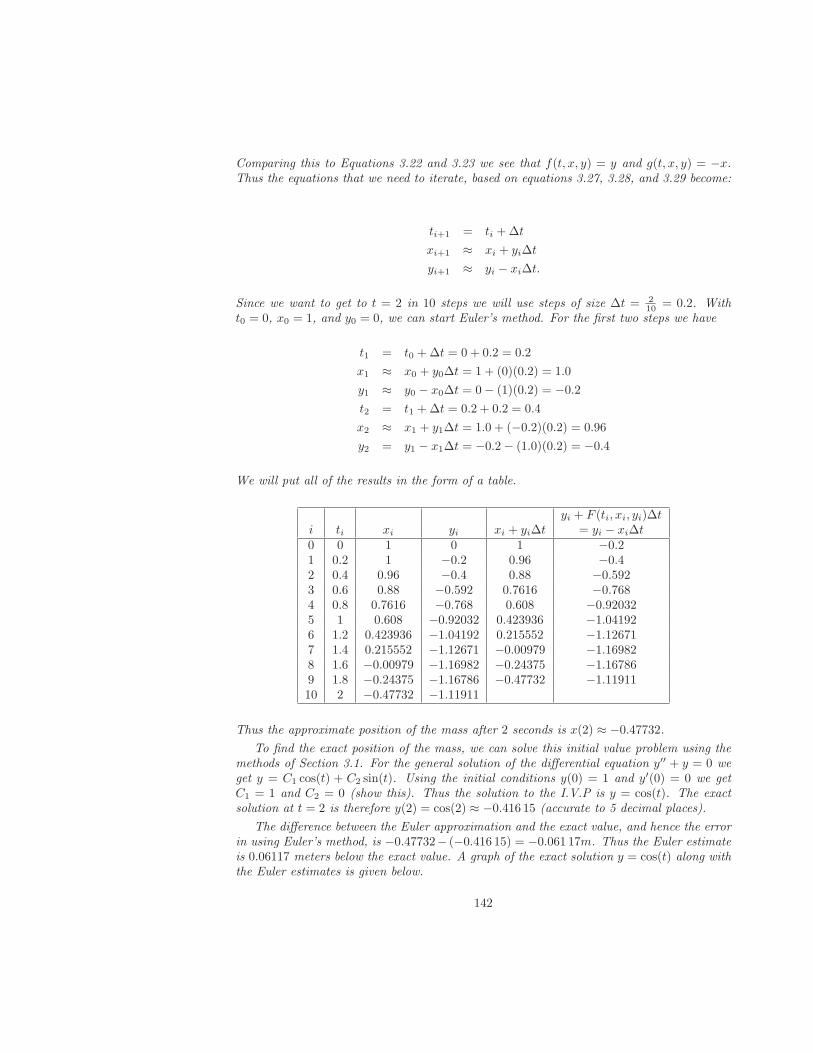
Comparing this to Equations 3.22 and 3.23 we see that f(t, x, y) = y and g(t, x, y) = −x.Thus the equations that we need to iterate, based on equations 3.27, 3.28, and 3.29 become:
ti+1 = ti +∆t
xi+1 ≈ xi + yi∆t
yi+1 ≈ yi − xi∆t.
Since we want to get to t = 2 in 10 steps we will use steps of size ∆t = 210 = 0.2. With
t0 = 0, x0 = 1, and y0 = 0, we can start Euler’s method. For the first two steps we have
t1 = t0 +∆t = 0 + 0.2 = 0.2
x1 ≈ x0 + y0∆t = 1 + (0)(0.2) = 1.0
y1 ≈ y0 − x0∆t = 0− (1)(0.2) = −0.2
t2 = t1 +∆t = 0.2 + 0.2 = 0.4
x2 ≈ x1 + y1∆t = 1.0 + (−0.2)(0.2) = 0.96
y2 = y1 − x1∆t = −0.2− (1.0)(0.2) = −0.4
We will put all of the results in the form of a table.
yi + F (ti, xi, yi)∆ti ti xi yi xi + yi∆t = yi − xi∆t0 0 1 0 1 −0.21 0.2 1 −0.2 0.96 −0.42 0.4 0.96 −0.4 0.88 −0.5923 0.6 0.88 −0.592 0.7616 −0.7684 0.8 0.7616 −0.768 0.608 −0.920325 1 0.608 −0.92032 0.423936 −1.041926 1.2 0.423936 −1.04192 0.215552 −1.126717 1.4 0.215552 −1.12671 −0.00979 −1.169828 1.6 −0.00979 −1.16982 −0.24375 −1.167869 1.8 −0.24375 −1.16786 −0.47732 −1.1191110 2 −0.47732 −1.11911
Thus the approximate position of the mass after 2 seconds is x(2) ≈ −0.47732.
To find the exact position of the mass, we can solve this initial value problem using themethods of Section 3.1. For the general solution of the differential equation y′′ + y = 0 weget y = C1 cos(t) + C2 sin(t). Using the initial conditions y(0) = 1 and y′(0) = 0 we getC1 = 1 and C2 = 0 (show this). Thus the solution to the I.V.P is y = cos(t). The exactsolution at t = 2 is therefore y(2) = cos(2) ≈ −0.416 15 (accurate to 5 decimal places).
The difference between the Euler approximation and the exact value, and hence the errorin using Euler’s method, is −0.47732− (−0.416 15) = −0.061 17m. Thus the Euler estimateis 0.06117 meters below the exact value. A graph of the exact solution y = cos(t) along withthe Euler estimates is given below.
142

QR O MRS O MSRS O P MS O MS O Q M ST S O Q M U
VU
Vy=cos(t) (solid line)
Euler estimates (boxes)
We see that the Euler estimates are above the graph of the exact solution when it ispositive, and below the graph of the exact solution when it is negative.
Order of Convergence
In Section 2.4 we discussed the concept of order of convergence; we briefly repeat someof that material here. Generally, as the step size ∆t gets smaller, the Euler estimates getbetter. Thus, in the previous example, if a step size of ∆t = 0.1 and 20 steps were chosen,instead of a step size of ∆t = 0.2 and 10 steps as was the case in the example, then the Eulerestimate at t = 2 would be more accurate (closer to the exact value at t = 2). The orderof convergence of a numerical method is a measure of how quickly the numerical estimateconverges to the exact solution as ∆t approaches 0. Euler’s method is a first order numericalmethod, that is, the order of convergence is 1. This means that if the stepsize is dividedby M then the error will also approximately be divided by M (as long as ∆t is sufficientlysmall to begin with). For example, if ∆t is reduced from 0.2 to 0.02 (divided by 10), thenone would expect the error in the Euler estimate to be approximately reduced by a powerof ten (divided by 10). Another way of saying this is that every time ∆t goes down by apower of ten, you get one more digit of accuracy in your estimate.
In general, a kth order numerical method would be one for which the error is dividedby Mk when the step size is divided by M (for ∆t sufficiently small). For example, if thestep size is divided by 10, then a second order method would reduce the error by 100 anda fourth order method would reduce the error by 10000. Equivalently, reducing the stepsize by one order of magnitude (one power of 10) gets you 2 more digits of accuracy with asecond order method, and 4 more digits of accuracy with a fourth order method.
It is impractical to do very many Euler steps when calculating by hand, so we will assumeyou have a calculator or computer software which can run Euler’s method for you for therest of this section.Note: With some software systems or calculators it is necessary to first write the equationin system form, as we have shown above. For example, if you are using one of the TIcalculators that has differential equation capability, you must convert to system form, butin Maple that is not necessary.
Example 3.5.2 Using the mass-spring system and initial conditions from Example 3.5.1(1kg mass, spring constant 1 n
m , no damping, y(0) = 1, y′(0) = 0), use Euler’s method
143
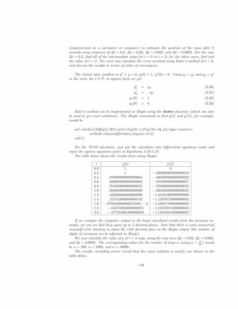
(implemented on a calculator or computer) to estimate the position of the mass after 2seconds using stepsizes of ∆t = 0.2, ∆t = 0.02, ∆t = 0.002, and ∆t = 0.0002. For the case∆t = 0.2, find all of the intermediate steps for t = 0 to t = 2; for the other cases, find justthe value at t = 2. For each case calculate the error involved using Euler’s method at t = 2,and discuss the results in terms of order of convergence.
The initial value problem is y′′ + y = 0, y(0) = 1, y′(0) = 0. Using y1 = y, and y2 = y′
to the write the I.V.P. in system form we get
y′1 = y2 (3.30)
y′2 = −y1 (3.31)
y1(0) = 1 (3.32)
y2(0) = 0 (3.33)
Euler’s method can be implemented in Maple using the dsolve function (which can alsobe used to get exact solutions). The Maple commands to find y(1) and y′(1), for example,would be
sol:=dsolve({diff(y(t),t$2)+y(t)=0,y(0)=1,D(y)(0)=0},y(t),type=numeric,method=classical[foreuler],stepsize=0.2);
sol(1);
For the TI-89 calculator, just put the calculator into differential equations mode andinput the system equations given in Equations 3.30-3.33.
The table below shows the results from using Maple:
t y(t) y′(t)0.0 1. 00.2 1. −.2000000000000000100.4 .959999999999999964 −.4000000000000000220.6 .880000000000000002 −.5919999999999999710.8 .761600000000000055 −.7680000000000000161.0 .608000000000000096 −.9203200000000000271.2 .423936000000000090 −1.041919999999999961.4 .215552000000000132 −1.126707200000000021.6 −.978944000000013180e− 2 −1.169817600000000001.8 −.243752960000000074 −1.167859712000000042.0 −.477324902400000028 −1.11910912000000007
If we compare the computer output to the hand calculated results from the previous ex-ample, we can see that they agree up to 5 decimal places. Note that there is some numericalroundoff error starting in about the 15th decimal place in the Maple output (the number ofdigits of accuracy can be adjusted in Maple).
We now calculate the value of y at t = 2 only, using the step sizes ∆t = 0.02, ∆t = 0.002,and ∆t = 0.0002. The corresponding values for the number of steps n (using n = 2
∆t) wouldbe n = 100, n = 1000, and n = 10000.
The results, including errors (recall that the exact solution is cos(2)) are shown in thetable below.
144
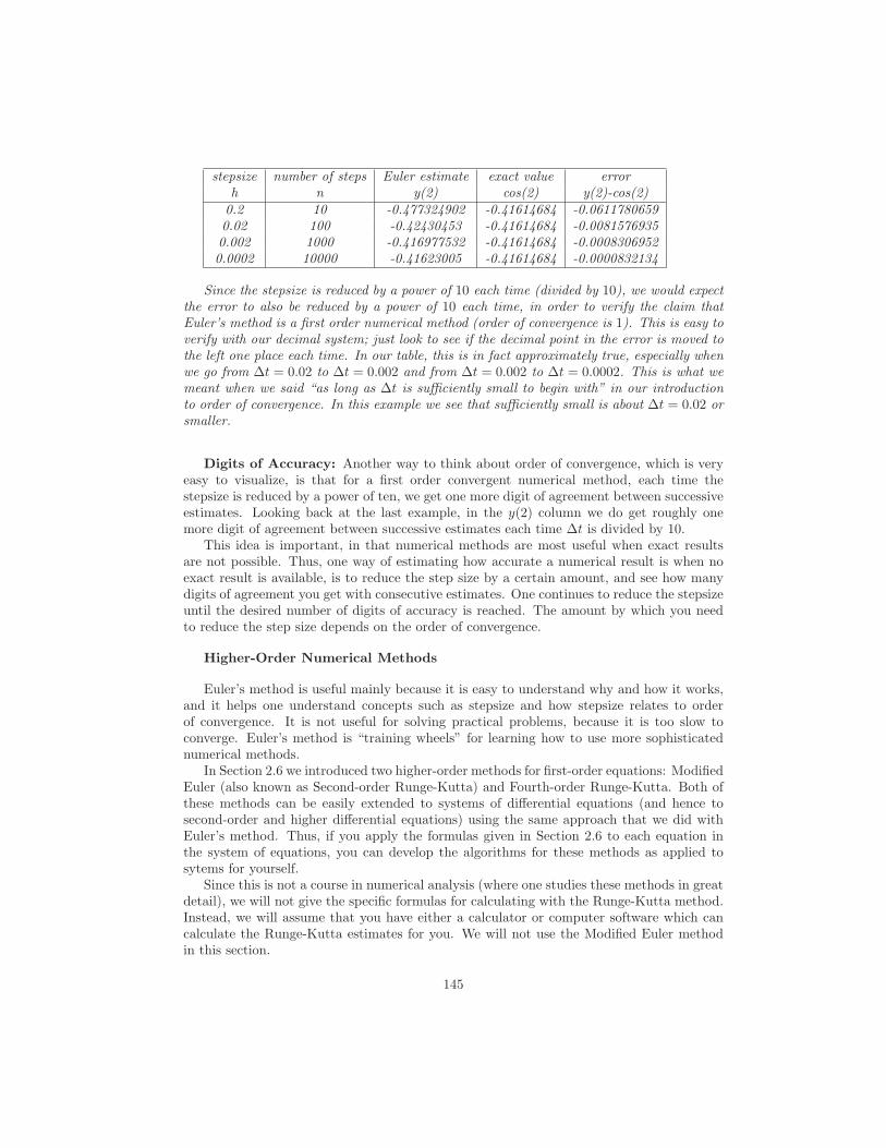
stepsize number of steps Euler estimate exact value errorh n y(2) cos(2) y(2)-cos(2)0.2 10 -0.477324902 -0.41614684 -0.06117806590.02 100 -0.42430453 -0.41614684 -0.00815769350.002 1000 -0.416977532 -0.41614684 -0.00083069520.0002 10000 -0.41623005 -0.41614684 -0.0000832134
Since the stepsize is reduced by a power of 10 each time (divided by 10), we would expectthe error to also be reduced by a power of 10 each time, in order to verify the claim thatEuler’s method is a first order numerical method (order of convergence is 1). This is easy toverify with our decimal system; just look to see if the decimal point in the error is moved tothe left one place each time. In our table, this is in fact approximately true, especially whenwe go from ∆t = 0.02 to ∆t = 0.002 and from ∆t = 0.002 to ∆t = 0.0002. This is what wemeant when we said “as long as ∆t is sufficiently small to begin with” in our introductionto order of convergence. In this example we see that sufficiently small is about ∆t = 0.02 orsmaller.
Digits of Accuracy: Another way to think about order of convergence, which is veryeasy to visualize, is that for a first order convergent numerical method, each time thestepsize is reduced by a power of ten, we get one more digit of agreement between successiveestimates. Looking back at the last example, in the y(2) column we do get roughly onemore digit of agreement between successive estimates each time ∆t is divided by 10.
This idea is important, in that numerical methods are most useful when exact resultsare not possible. Thus, one way of estimating how accurate a numerical result is when noexact result is available, is to reduce the step size by a certain amount, and see how manydigits of agreement you get with consecutive estimates. One continues to reduce the stepsizeuntil the desired number of digits of accuracy is reached. The amount by which you needto reduce the step size depends on the order of convergence.
Higher-Order Numerical Methods
Euler’s method is useful mainly because it is easy to understand why and how it works,and it helps one understand concepts such as stepsize and how stepsize relates to orderof convergence. It is not useful for solving practical problems, because it is too slow toconverge. Euler’s method is “training wheels” for learning how to use more sophisticatednumerical methods.
In Section 2.6 we introduced two higher-order methods for first-order equations: ModifiedEuler (also known as Second-order Runge-Kutta) and Fourth-order Runge-Kutta. Both ofthese methods can be easily extended to systems of differential equations (and hence tosecond-order and higher differential equations) using the same approach that we did withEuler’s method. Thus, if you apply the formulas given in Section 2.6 to each equation inthe system of equations, you can develop the algorithms for these methods as applied tosytems for yourself.
Since this is not a course in numerical analysis (where one studies these methods in greatdetail), we will not give the specific formulas for calculating with the Runge-Kutta method.Instead, we will assume that you have either a calculator or computer software which cancalculate the Runge-Kutta estimates for you. We will not use the Modified Euler methodin this section.
145
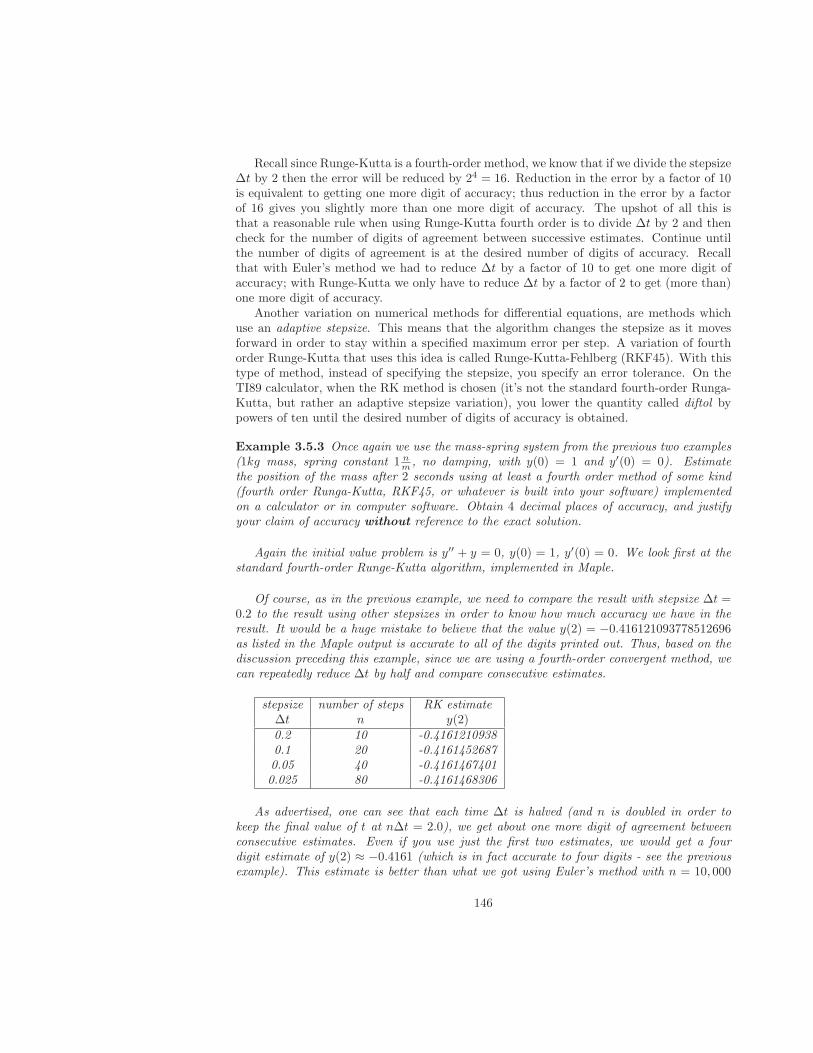
Recall since Runge-Kutta is a fourth-order method, we know that if we divide the stepsize∆t by 2 then the error will be reduced by 24 = 16. Reduction in the error by a factor of 10is equivalent to getting one more digit of accuracy; thus reduction in the error by a factorof 16 gives you slightly more than one more digit of accuracy. The upshot of all this isthat a reasonable rule when using Runge-Kutta fourth order is to divide ∆t by 2 and thencheck for the number of digits of agreement between successive estimates. Continue untilthe number of digits of agreement is at the desired number of digits of accuracy. Recallthat with Euler’s method we had to reduce ∆t by a factor of 10 to get one more digit ofaccuracy; with Runge-Kutta we only have to reduce ∆t by a factor of 2 to get (more than)one more digit of accuracy.
Another variation on numerical methods for differential equations, are methods whichuse an adaptive stepsize. This means that the algorithm changes the stepsize as it movesforward in order to stay within a specified maximum error per step. A variation of fourthorder Runge-Kutta that uses this idea is called Runge-Kutta-Fehlberg (RKF45). With thistype of method, instead of specifying the stepsize, you specify an error tolerance. On theTI89 calculator, when the RK method is chosen (it’s not the standard fourth-order Runga-Kutta, but rather an adaptive stepsize variation), you lower the quantity called diftol bypowers of ten until the desired number of digits of accuracy is obtained.
Example 3.5.3 Once again we use the mass-spring system from the previous two examples(1kg mass, spring constant 1 n
m , no damping, with y(0) = 1 and y′(0) = 0). Estimatethe position of the mass after 2 seconds using at least a fourth order method of some kind(fourth order Runga-Kutta, RKF45, or whatever is built into your software) implementedon a calculator or in computer software. Obtain 4 decimal places of accuracy, and justifyyour claim of accuracy without reference to the exact solution.
Again the initial value problem is y′′ + y = 0, y(0) = 1, y′(0) = 0. We look first at thestandard fourth-order Runge-Kutta algorithm, implemented in Maple.
Of course, as in the previous example, we need to compare the result with stepsize ∆t =0.2 to the result using other stepsizes in order to know how much accuracy we have in theresult. It would be a huge mistake to believe that the value y(2) = −0.416121093778512696as listed in the Maple output is accurate to all of the digits printed out. Thus, based on thediscussion preceding this example, since we are using a fourth-order convergent method, wecan repeatedly reduce ∆t by half and compare consecutive estimates.
stepsize number of steps RK estimate∆t n y(2)0.2 10 -0.41612109380.1 20 -0.41614526870.05 40 -0.41614674010.025 80 -0.4161468306
As advertised, one can see that each time ∆t is halved (and n is doubled in order tokeep the final value of t at n∆t = 2.0), we get about one more digit of agreement betweenconsecutive estimates. Even if you use just the first two estimates, we would get a fourdigit estimate of y(2) ≈ −0.4161 (which is in fact accurate to four digits - see the previousexample). This estimate is better than what we got using Euler’s method with n = 10, 000
146
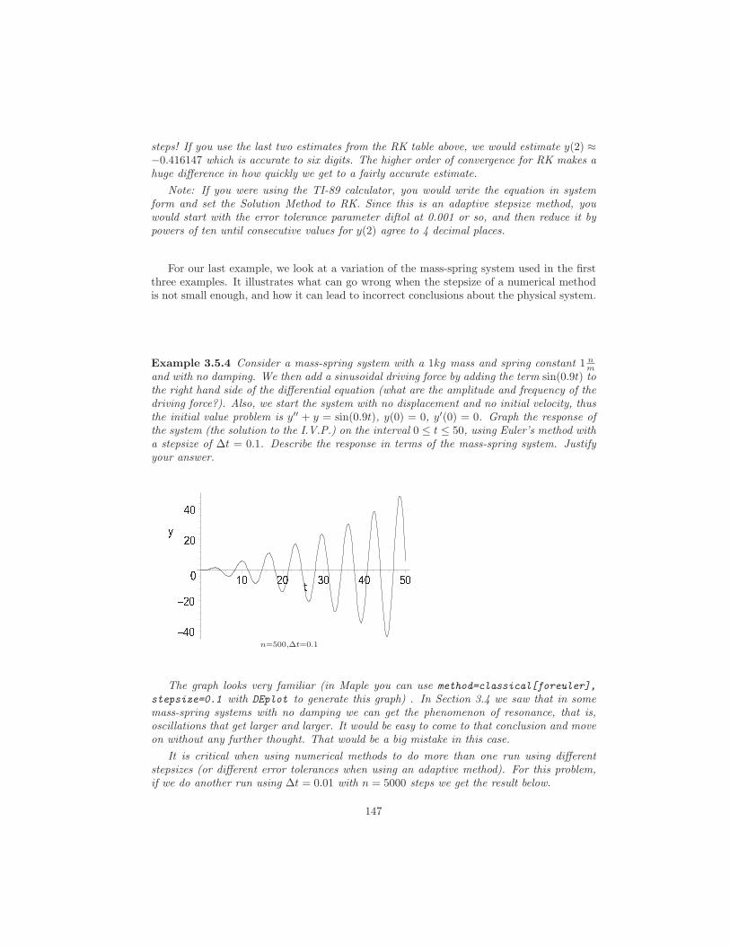
steps! If you use the last two estimates from the RK table above, we would estimate y(2) ≈−0.416147 which is accurate to six digits. The higher order of convergence for RK makes ahuge difference in how quickly we get to a fairly accurate estimate.
Note: If you were using the TI-89 calculator, you would write the equation in systemform and set the Solution Method to RK. Since this is an adaptive stepsize method, youwould start with the error tolerance parameter diftol at 0.001 or so, and then reduce it bypowers of ten until consecutive values for y(2) agree to 4 decimal places.
For our last example, we look at a variation of the mass-spring system used in the firstthree examples. It illustrates what can go wrong when the stepsize of a numerical methodis not small enough, and how it can lead to incorrect conclusions about the physical system.
Example 3.5.4 Consider a mass-spring system with a 1kg mass and spring constant 1 nm
and with no damping. We then add a sinusoidal driving force by adding the term sin(0.9t) tothe right hand side of the differential equation (what are the amplitude and frequency of thedriving force?). Also, we start the system with no displacement and no initial velocity, thusthe initial value problem is y′′ + y = sin(0.9t), y(0) = 0, y′(0) = 0. Graph the response ofthe system (the solution to the I.V.P.) on the interval 0 ≤ t ≤ 50, using Euler’s method witha stepsize of ∆t = 0.1. Describe the response in terms of the mass-spring system. Justifyyour answer.
u v wu x w wx wv wy z w x w { w v w | w}n=500,∆t=0.1
The graph looks very familiar (in Maple you can use method=classical[foreuler],
stepsize=0.1 with DEplot to generate this graph) . In Section 3.4 we saw that in somemass-spring systems with no damping we can get the phenomenon of resonance, that is,oscillations that get larger and larger. It would be easy to come to that conclusion and moveon without any further thought. That would be a big mistake in this case.
It is critical when using numerical methods to do more than one run using differentstepsizes (or different error tolerances when using an adaptive method). For this problem,if we do another run using ∆t = 0.01 with n = 5000 steps we get the result below.
147
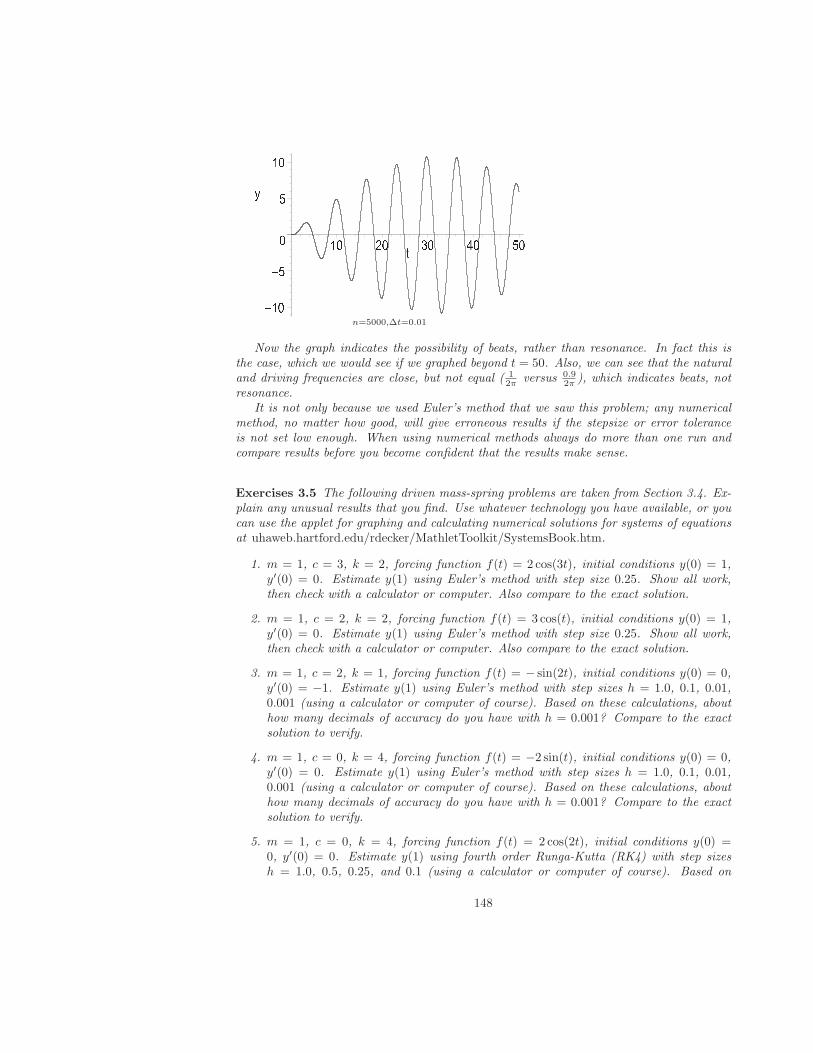
u z wu | w|z wy z w x w { w v w | w}n=5000,∆t=0.01
Now the graph indicates the possibility of beats, rather than resonance. In fact this isthe case, which we would see if we graphed beyond t = 50. Also, we can see that the naturaland driving frequencies are close, but not equal ( 1
2π versus 0.92π ), which indicates beats, not
resonance.It is not only because we used Euler’s method that we saw this problem; any numerical
method, no matter how good, will give erroneous results if the stepsize or error toleranceis not set low enough. When using numerical methods always do more than one run andcompare results before you become confident that the results make sense.
Exercises 3.5 The following driven mass-spring problems are taken from Section 3.4. Ex-plain any unusual results that you find. Use whatever technology you have available, or youcan use the applet for graphing and calculating numerical solutions for systems of equationsat uhaweb.hartford.edu/rdecker/MathletToolkit/SystemsBook.htm.
1. m = 1, c = 3, k = 2, forcing function f(t) = 2 cos(3t), initial conditions y(0) = 1,y′(0) = 0. Estimate y(1) using Euler’s method with step size 0.25. Show all work,then check with a calculator or computer. Also compare to the exact solution.
2. m = 1, c = 2, k = 2, forcing function f(t) = 3 cos(t), initial conditions y(0) = 1,y′(0) = 0. Estimate y(1) using Euler’s method with step size 0.25. Show all work,then check with a calculator or computer. Also compare to the exact solution.
3. m = 1, c = 2, k = 1, forcing function f(t) = − sin(2t), initial conditions y(0) = 0,y′(0) = −1. Estimate y(1) using Euler’s method with step sizes h = 1.0, 0.1, 0.01,0.001 (using a calculator or computer of course). Based on these calculations, abouthow many decimals of accuracy do you have with h = 0.001? Compare to the exactsolution to verify.
4. m = 1, c = 0, k = 4, forcing function f(t) = −2 sin(t), initial conditions y(0) = 0,y′(0) = 0. Estimate y(1) using Euler’s method with step sizes h = 1.0, 0.1, 0.01,0.001 (using a calculator or computer of course). Based on these calculations, abouthow many decimals of accuracy do you have with h = 0.001? Compare to the exactsolution to verify.
5. m = 1, c = 0, k = 4, forcing function f(t) = 2 cos(2t), initial conditions y(0) =0, y′(0) = 0. Estimate y(1) using fourth order Runga-Kutta (RK4) with step sizesh = 1.0, 0.5, 0.25, and 0.1 (using a calculator or computer of course). Based on
148
these calculations, about how many decimals of accuracy do you have with h = 0.1?Compare to the exact solution to verify.
6. m = 1, c = 0, k = 100, forcing function f(t) = 40 cos(9t), initial conditions y(0) =0, y′(0) = 0. Estimate y(1) using fourth order Runga-Kutta (RK4) with step sizesh = 1.0, 0.5, 0.25, and 0.1 (using a calculator or computer of course). Based onthese calculations, about how many decimals of accuracy do you have with h = 0.1?Compare to the exact solution to verify.
7. m = 1, c = 0, k = 4, forcing function f(t) = 2 cos(2t), initial conditions y(0) = 0,y′(0) = 0. Estimate y(1) using an adaptive step size algorithm (such as RK on theTI-89) with error tolerance 0.1, 0.01, 0.001, and 0.0001 (diftol on the TI-89). Basedon these calculations, about how many decimals of accuracy do you have with errortolerance 0.0001? Compare to the exact solution to verify.
8. m = 1, c = 0, k = 100, forcing function f(t) = 40 cos(9t), initial conditions y(0) = 0,y′(0) = 0. Estimate y(1) using an adaptive step size algorithm (such as RK on theTI-89) with error tolerance 0.1, 0.01, 0.001, and 0.0001 (diftol on the TI-89). Basedon these calculations, about how many decimals of accuracy do you have with errortolerance 0.0001? Compare to the exact solution to verify.
149
3.6 Qualitative Methods and the Phase Plane
We now turn to methods for obtaining information from second-order differential equationswithout solving them explicitly (as in Sections 3.1 and 3.3), or numerically (as in Section3.5). To understand the qualitative behavior of solutions of second-order equations, you willneed to learn about some new types of graphs called vector fields, direction fields and phaseplots. These expand on the ideas of the slope field and the phase line, defined for first-orderequations in Chapter 2. We will find that they are most useful when the differential equationbeing studied is autonomous; that is, is of the form x′′ = F (x, x′).
The Phase Plane
We saw in the last section that in order to apply Euler’s method to a second-orderdifferential equation, we need to calculate not just the position x but also the velocity x′ ateach step. This is because knowing the value of x(t0) at some time t = t0 does not determinethe value of x′(t0) for second-order equations. This differs from the first-order case becausewhen we write a first-order equation in the form x′(t) = f(t, x(t)) we get x′(t0) = f(t0, x(t0))which determines x′(t0) without having to solve the differential equation itself. For second-order equations we can write x′′(t) = F (t, x(t), x′(t)), but this does not help us determinex′(t0) when we know x(t0) (though it does determine x′′(t0) when we know x(t0) and x′(t0)as we saw in the last section).
The consequence of the above discussion is that for second-order equations we can thinkof the solution as consisting of a list of corresponding t, x(t), and x′(t) values. Again, ifwe look back at the last section on numerical methods, we see that in fact this is preciselywhat we generate using Euler’s method (see Examples 3.5.1 and 3.5.2). So far we have justlooked at the t versus x(t) graph when graphing the solution to a second-order differentialequation. We could, however, just as easily look at a t versus x′(t) graph or an x(t) versusx′(t) graph. We will refer to the t versus x(t) and t versus x′(t) graphs as time plots, andthe x(t) versus x′(t) graph as the phase plot. A phase plot is an example of a parametricplot, which you may have studied in a precalculus or calculus course. When the coordinateplane is labelled with x along the horizontal axis and x′ along the vertical axis, we refer tothat coordinate plane as the phase plane.
Furthermore, recall from the last section that it is often convenient to write a second-order differential equation as a first-order system. When we define new variables x1 = x,and x2 = x′, then a phase plot would be a plot of x2 versus x1. In Chapter 4 where westudy systems in and of themselves, plots of x2 versus x1 will also be called phase plots.
Example 3.6.1 For each of the following initial value problems, solve the differential equa-tion to obtain x(t) and x′(t), and sketch both time plots (t versus x(t) and t versus x′(t))and the phase plot ( x(t) versus x′(t)). Use the interval 0 ≤ t ≤ 20. Relate the results tomass-spring systems.
a) x′′ + 4x = 0, x(0) = 0, x′(0) = 2b) x′′ + 0.2x′ + 4.01x = 0, x(0) = 0, x′(0) = 2c) x′′ + 4x = sin(1.6t), x(0) = 0, x′(0) = 0
Each equation can be solved for x(t), using the methods of sections 3.1 (for a and b) and3.3 (for c). Then for each case simply differentiate x(t) to find x′(t). We get
a) x = sin(2t), x′ = ddt sin(2t) = 2 cos(2t)
150
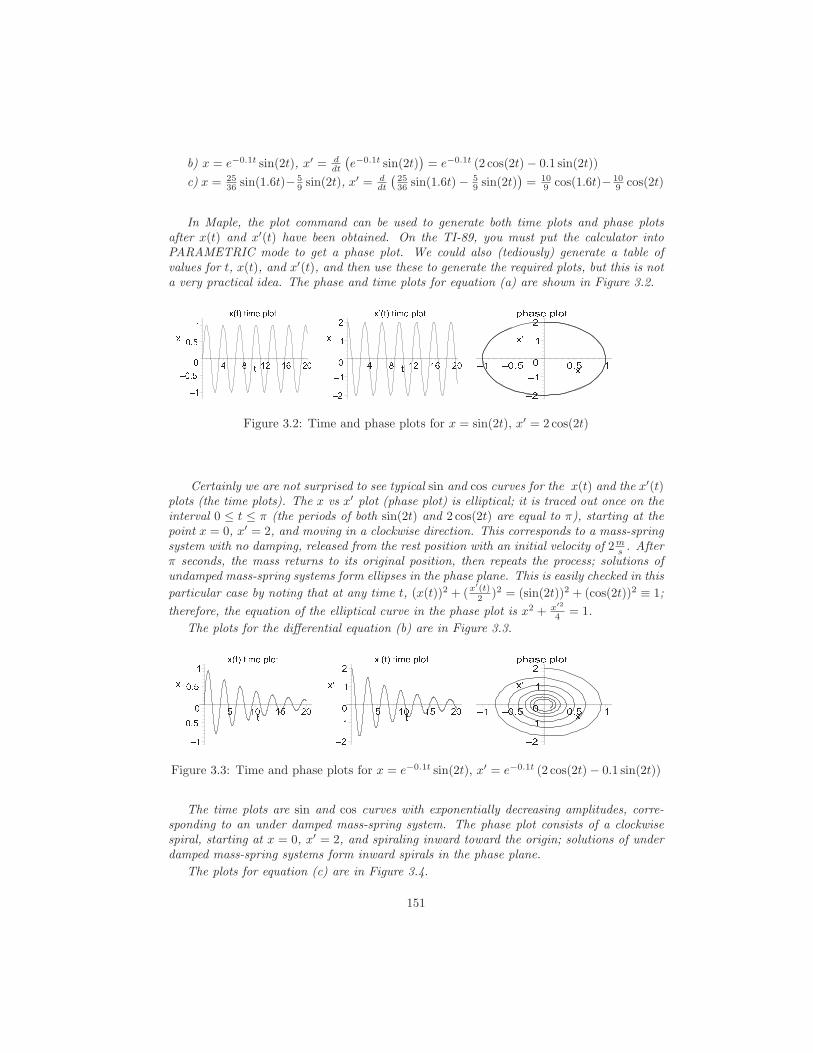
b) x = e−0.1t sin(2t), x′ = ddt
(e−0.1t sin(2t)
)= e−0.1t (2 cos(2t)− 0.1 sin(2t))
c) x = 2536 sin(1.6t)− 5
9 sin(2t), x′ = d
dt
(2536 sin(1.6t)− 5
9 sin(2t))= 10
9 cos(1.6t)− 109 cos(2t)
In Maple, the plot command can be used to generate both time plots and phase plotsafter x(t) and x′(t) have been obtained. On the TI-89, you must put the calculator intoPARAMETRIC mode to get a phase plot. We could also (tediously) generate a table ofvalues for t, x(t), and x′(t), and then use these to generate the required plots, but this is nota very practical idea. The phase and time plots for equation (a) are shown in Figure 3.2.~ � � � � � � � � � � �� �� � � � �� � � �~ � � � � � � � �� � � � � � � � � � � � � �� �� �� ��� ¡ � � � ¢ � �� £ ¤ ¥ ¦ § £ ¨ © ª« ¬« ® ¬¯ °« « ® ± ² ® ± ² ¯
Figure 3.2: Time and phase plots for x = sin(2t), x′ = 2 cos(2t)
Certainly we are not surprised to see typical sin and cos curves for the x(t) and the x′(t)plots (the time plots). The x vs x′ plot (phase plot) is elliptical; it is traced out once on theinterval 0 ≤ t ≤ π (the periods of both sin(2t) and 2 cos(2t) are equal to π), starting at thepoint x = 0, x′ = 2, and moving in a clockwise direction. This corresponds to a mass-springsystem with no damping, released from the rest position with an initial velocity of 2m
s . Afterπ seconds, the mass returns to its original position, then repeats the process; solutions ofundamped mass-spring systems form ellipses in the phase plane. This is easily checked in this
particular case by noting that at any time t, (x(t))2 + (x′(t)2 )2 = (sin(2t))2 + (cos(2t))2 ≡ 1;
therefore, the equation of the elliptical curve in the phase plot is x2 + x′2
4 = 1.
The plots for the differential equation (b) are in Figure 3.3.³ ´ µ ¶ µ · ¸ ¹ º » ¼ µ½ ¾½ ¿ À Á ¿¿ À Á ¾³ Á ¾ ¿ ¾ Á  ¿µ Ã Ä Å Æ Ç Æ È É Ê Ë Ì Í ÆÎ ÏÎ ÐÑ ÐÏÃ Ä Ò Ð Ñ Ð Ò Ï ÑÆ £ ¤ ¥ ¦ § £ ¨ © ª« ¬« ® ¬¯ °« « ® ± ² ® ± ² ¯Figure 3.3: Time and phase plots for x = e−0.1t sin(2t), x′ = e−0.1t (2 cos(2t)− 0.1 sin(2t))
The time plots are sin and cos curves with exponentially decreasing amplitudes, corre-sponding to an under damped mass-spring system. The phase plot consists of a clockwisespiral, starting at x = 0, x′ = 2, and spiraling inward toward the origin; solutions of underdamped mass-spring systems form inward spirals in the phase plane.
The plots for equation (c) are in Figure 3.4.
151
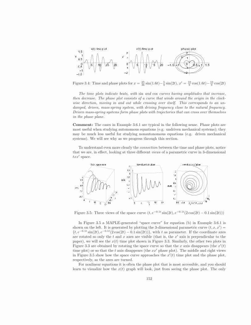
³ ´ µ ¶ µ · ¸ ¹ º » ¼ µ½ ¾ À Á½ ¾½ ¿ À Á ¿¿ À Á ¾¾ À Á³ Á ¾ ¿ ¾ Á  ¿µ Ã Ä Å Æ Ç Æ È É Ê Ë Ì Í ÆÎ ÏÎ ÐÑ ÐÏÃ Ä Ò Ð Ñ Ð Ò Ï ÑÆ Ó Ô Õ Ö × Ó Ø Ù ÚÛ ÜÛ ÝÞ ÝÜß àÛ Ý á â Û Ý Þ á â Ý Ý á âßFigure 3.4: Time and phase plots for x = 25
36 sin(1.6t)− 59 sin(2t), x
′ = 109 cos(1.6t)− 10
9 cos(2t)
The time plots indicate beats, with sin and cos curves having amplitudes that increase,then decrease. The phase plot consists of a curve that winds around the origin in the clock-wise direction, moving in and out while crossing over itself. This corresponds to an un-damped, driven, mass-spring system, with driving frequency close to the natural frequency.Driven mass-spring systems form phase plots with trajectories that can cross over themselvesin the phase plane.
Comment: The cases in Example 3.6.1 are typical in the following sense. Phase plots aremost useful when studying autonomous equations (e.g. undriven mechanical systems); theymay be much less useful for studying nonautonomous equations (e.g. driven mechanicalsystems). We will see why as we progress through this section.
To understand even more clearly the connection between the time and phase plots, noticethat we are, in effect, looking at three different views of a parametric curve in 3-dimensionaltxx′ space.ã ä å æ ç è é ê ë ì í ì î ï ð í
ñ ò ó ñ ó ò ô ñõ ö ñ è ÷ö ñ è øñ ñ è ø ñ è ÷ùö ó è òö óö ñ è ò ññ è ò óó è ò ôå ù ú å õ û ü ý þ ÿ � � � ý � � � � � � � � � ý � � � �� � � � � � �� � �� � � � � � � � � � � � � � � � � � � � � � � �
� �! � �" � # $ " � # % � � # ! � # % � # & � # $�" # '" " � # ' �� # ' # ' !( � ) ( �Figure 3.5: Three views of the space curve (t, e−0.1t sin(2t), e−0.1t(2 cos(2t)− 0.1 sin(2t)))
In Figure 3.5 a MAPLE-generated “space curve” for equation (b) in Example 3.6.1 isshown on the left. It is generated by plotting the 3-dimensional parametric curve (t, x, x′) =(t, e−0.1t sin(2t), e−0.1t(2 cos(2t)− 0.1 sin(2t))
), with t as parameter. If the coordinate axes
are rotated so only the t and x axes are visible (that is, the x′ axis is perpendicular to thepaper), we will see the x(t) time plot shown in Figure 3.3. Similarly, the other two plots inFigure 3.3 are obtained by rotating the space curve so that the x axis disappears (the x′(t)time plot) or so that the t axis disappears (the xx′ phase plot). The middle and right viewsin Figure 3.5 show how the space curve approaches the x′(t) time plot and the phase plot,respectively, as the axes are turned.
For nonlinear equations it is often the phase plot that is most accessible, and you shouldlearn to visualize how the x(t) graph will look, just from seeing the phase plot. The only
152
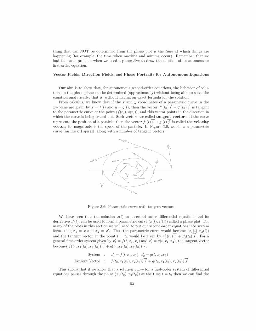
thing that can NOT be determined from the phase plot is the time at which things arehappening (for example, the time when maxima and minima occur). Remember that wehad the same problem when we used a phase line to draw the solution of an autonomousfirst-order equation.
Vector Fields, Direction Fields, and Phase Portraits for Autonomous Equations
Our aim is to show that, for autonomous second-order equations, the behavior of solu-tions in the phase plane can be determined (approximately) without being able to solve theequation analytically; that is, without having an exact formula for the solution.
From calculus, we know that if the x and y coordinates of a parametric curve in the
xy-plane are given by x = f(t) and y = g(t), then the vector f ′(t0)−→i + g′(t0)
−→j is tangent
to the parametric curve at the point (f(t0), g(t0)), and this vector points in the direction inwhich the curve is being traced out. Such vectors are called tangent vectors. If the curve
represents the position of a particle, then the vector f ′(t)−→i + g′(t)
−→j is called the velocity
vector; its magnitude is the speed of the particle. In Figure 3.6, we show a parametriccurve (an inward spiral), along with a number of tangent vectors.
Figure 3.6: Parametric curve with tangent vectors
We have seen that the solution x(t) to a second order differential equation, and itsderivative x′(t), can be used to form a parametric curve (x(t), x′(t)) called a phase plot. Formany of the plots in this section we will need to put our second-order equations into systemform using x1 = x and x2 = x′. Thus the parametric curve would become (x1(t), x2(t))
and the tangent vector at the point t = t0 would be given by x′1(t0)
−→i + x′
2(t0)−→j . For a
general first-order system given by x′1 = f(t, x1, x2) and x′
2 = g(t, x1, x2), the tangent vector
becomes f(t0, x1(t0), x2(t0))−→i + g(t0, x1(t0), x2(t0))
−→j .
System : x′1 = f(t, x1, x2), x
′2 = g(t, x1, x2)
Tangent Vector : f(t0, x1(t0), x2(t0))−→i + g(t0, x1(t0), x2(t0))
−→j
This shows that if we know that a solution curve for a first-order system of differentialequations passes through the point (x1(t0), x2(t0)) at the time t = t0 then we can find the
153
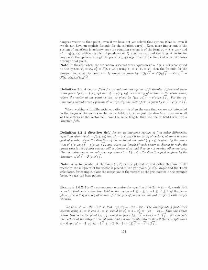
tangent vector at that point, even if we have not yet solved that system (that is, even ifwe do not have an explicit formula for the solution curve). Even more important, if thesystem of equations is autonomous (the equation system is of the form x′
1 = f(x1, x2) andx′2 = g(x1, x2) with no explicit dependence on t), then we can find the tangent vector for
any curve that passes through the point (x1, x2) regardless of the time t at which it passesthrough that point.Note: In the case where the autonomous second-order equation x′′ = F (t, x, x′) is convertedto the system x′
1 = x2, x′2 = F (t, x1, x2) using x1 = x, x2 = x′, then the formula for the
tangent vector at the point t = t0 would be given by x′(t0)−→i + x′′(t0)
−→j = x′(t0)
−→i +
F (t0, x(t0), x′(t0))
−→j .
Definition 3.1 A vector field for an autonomous system of first-order differential equa-tions given by x′
1 = f(x1, x2) and x′2 = g(x1, x2) is an array of vectors in the phase plane,
where the vector at the point (x1, x2) is given by f(x1, x2)−→i + g(x1, x2)
−→j . For the au-
tonomous second-order equation x′′ = F (x, x′), the vector field is given by x′−→i +F (x, x′)−→j .
When working with differential equations, it is often the case that we are not interestedin the length of the vectors in the vector field, but rather just the direction. If we make allof the vectors in the vector field have the same length, then the vector field turns into adirection field.
Definition 3.2 A direction field for an autonomous system of first-order differentialequations given by x′
1 = f(x1, x2) and x′2 = g(x1, x2) is an array of vectors, at some selected
grid of points, where the direction of the vector at the point (x1, x2) is given by the direc-
tion of f(x1, x2)−→i + g(x1, x2)
−→j , and where the length of each vector is chosen to make the
graph easy to read (most vectors will be shortened so that they do not overlap other vectors).For the autonomous second-order equation x′′ = F (x, x′), the direction field is given by the
direction of x′−→i + F (x, x′)−→j .
Note: A vector located at the point (x, x′) can be plotted so that either the base of thevector or the midpoint of the vector is placed at the grid point (x, x′). Maple and the TI-89calculator, for example, place the midpoints of the vectors at the grid points; in the examplebelow we use the base points.
Example 3.6.2 For the autonomous second-order equation x′′ + 2x′ + 2x = 0, create botha vector field, and a direction field in the region −1 ≤ x ≤ 1, −1 ≤ x′ ≤ 1 of the phaseplane. Use a 3 by 3 array of vectors (for the grid of points, use the ordered pairs with integervalues).
We have x′′ = −2x − 2x′ so that F (x, x′) = −2x − 2x′. The corresponding first-ordersystem using x1 = x and x2 = x′ would be x′
1 = x2, x′2 = −2x1 − 2x2. Thus the vector
whose base is at the point (x1, x2) would be given by x′−→i + (−2x − 2x′)−→j . We calculate
the vectors at the integer ordered pairs and put the results into Table 3.2 (for example when
x = 0 and x′ = −1 we get −1−→i + (−2 · 0− 2 · (−1))
−→j = −−→
i + 2−→j ).
154
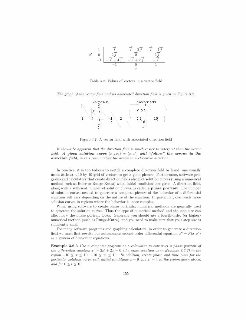
1−→i
−→i − 2
−→j
−→i − 4
−→j
x′ 0 2−→j
−→0 −2
−→j
−1 −−→i + 4
−→j −−→
i + 2−→j −−→
i−1 0 1
x
Table 3.2: Values of vectors in a vector field
The graph of the vector field and its associated direction field is given in Figure 3.7.* + , - . / 0 1 + 2 34 54 64 7 76 58 94 6 4 7 7 68 3 1 / + , - 1 . : 0 1 + 2 3
4 74 ; < =; < = 78 94 7 4 ; < = ; < = 78Figure 3.7: A vector field with associated direction field
It should be apparent that the direction field is much easier to interpret than the vectorfield. A given solution curve (x1, x2) = (x, x′) will “follow” the arrows in the
direction field, in this case circling the origin in a clockwise direction.
In practice, it is too tedious to sketch a complete direction field by hand; one usuallyneeds at least a 10 by 10 grid of vectors to get a good picture. Furthermore, software pro-grams and calculators that create direction fields also plot solution curves (using a numericalmethod such as Euler or Runge-Kutta) when initial conditions are given. A direction field,along with a sufficient number of solution curves, is called a phase portrait. The numberof solution curves needed to generate a complete picture of the behavior of a differentialequation will vary depending on the nature of the equation. In particular, one needs moresolution curves in regions where the behavior is more complex.
When using software to create phase portraits, numerical methods are generally usedto generate the solution curves. Thus the type of numerical method and the step size canaffect how the phase portrait looks. Generally you should use a fourth-order (or higher)numerical method (such as Runge-Kutta), and you need to make sure that your step size issufficiently small.
For many software programs and graphing calculators, in order to generate a directionfield we must first rewrite our autonomous second-order differential equation x′′ = F (x, x′)as a system of first-order equations.
Example 3.6.3 Use a computer program or a calculator to construct a phase portrait ofthe differential equation x′′ + 2x′ + 2x = 0 (the same equation as in Example 3.6.2) in theregion −10 ≤ x ≤ 10, −10 ≤ x′ ≤ 10. In addition, create phase and time plots for theparticular solution curve with initial conditions x = 9 and x′ = 4 in the region given above,and for 0 ≤ t ≤ 10.
155
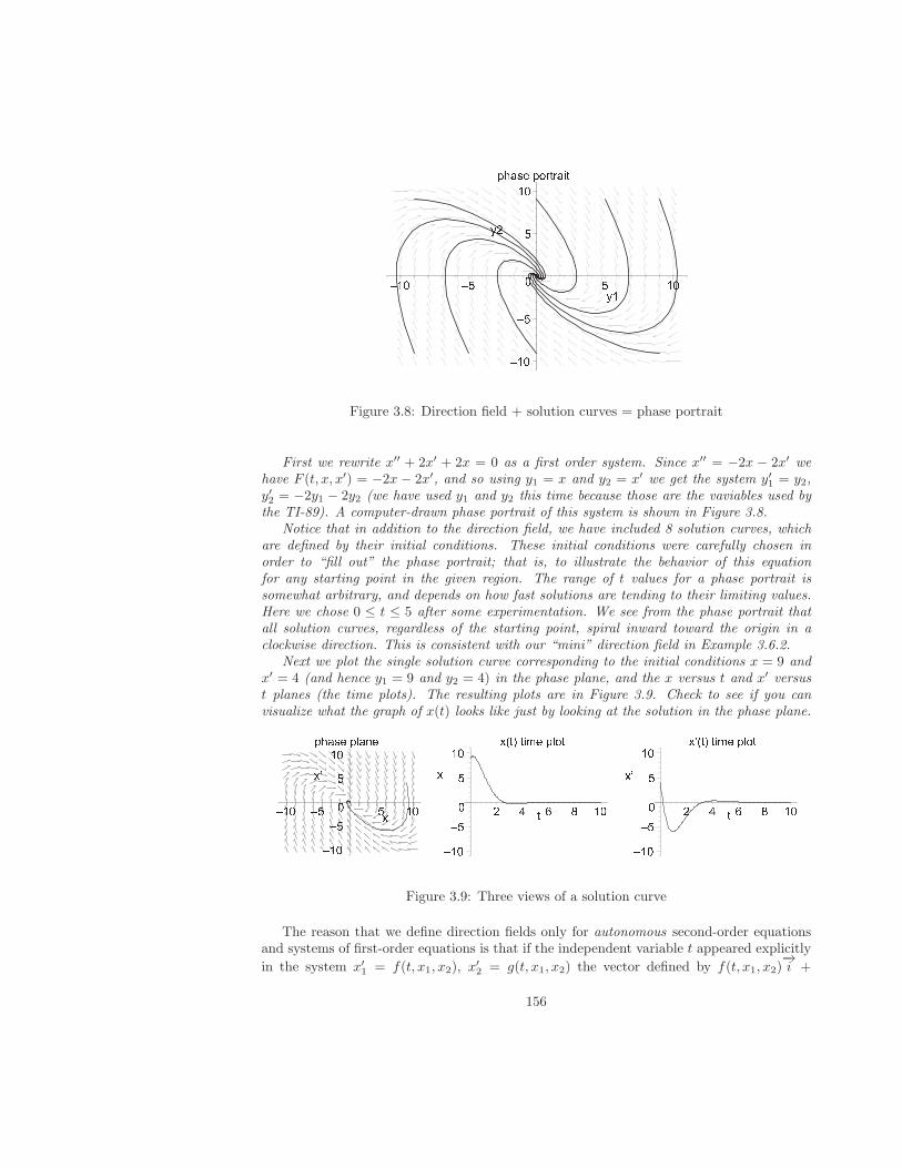
> ? @ A + > . / - / @ 1 -4 7 ;4 = ;=7 ;8 64 7 ; 4 = = 7 ;8 7
Figure 3.8: Direction field + solution curves = phase portrait
First we rewrite x′′ + 2x′ + 2x = 0 as a first order system. Since x′′ = −2x − 2x′ wehave F (t, x, x′) = −2x − 2x′, and so using y1 = x and y2 = x′ we get the system y′1 = y2,y′2 = −2y1 − 2y2 (we have used y1 and y2 this time because those are the vaviables used bythe TI-89). A computer-drawn phase portrait of this system is shown in Figure 3.8.
Notice that in addition to the direction field, we have included 8 solution curves, whichare defined by their initial conditions. These initial conditions were carefully chosen inorder to “fill out” the phase portrait; that is, to illustrate the behavior of this equationfor any starting point in the given region. The range of t values for a phase portrait issomewhat arbitrary, and depends on how fast solutions are tending to their limiting values.Here we chose 0 ≤ t ≤ 5 after some experimentation. We see from the phase portrait thatall solution curves, regardless of the starting point, spiral inward toward the origin in aclockwise direction. This is consistent with our “mini” direction field in Example 3.6.2.
Next we plot the single solution curve corresponding to the initial conditions x = 9 andx′ = 4 (and hence y1 = 9 and y2 = 4) in the phase plane, and the x versus t and x′ versust planes (the time plots). The resulting plots are in Figure 3.9. Check to see if you canvisualize what the graph of x(t) looks like just by looking at the solution in the phase plane.B C D E F B G D H F
I J KI L KLJ KM NI J K I L L J KM M O P Q P R S F B G T PI J KI L KLJ KM U V W X J KP M N O P Q P R S F B G T P
I J KI L KLJ KM N U V W X J KPFigure 3.9: Three views of a solution curve
The reason that we define direction fields only for autonomous second-order equationsand systems of first-order equations is that if the independent variable t appeared explicitly
in the system x′1 = f(t, x1, x2), x′
2 = g(t, x1, x2) the vector defined by f(t, x1, x2)−→i +
156
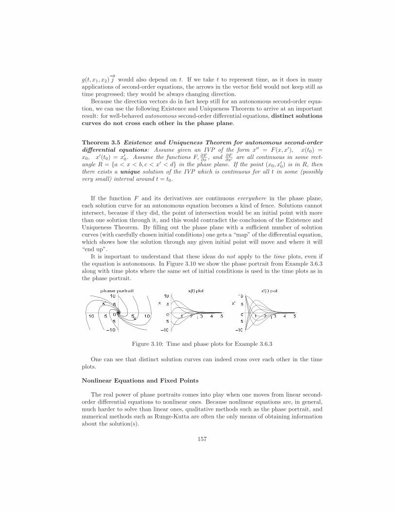
g(t, x1, x2)−→j would also depend on t. If we take t to represent time, as it does in many
applications of second-order equations, the arrows in the vector field would not keep still astime progressed; they would be always changing direction.
Because the direction vectors do in fact keep still for an autonomous second-order equa-tion, we can use the following Existence and Uniqueness Theorem to arrive at an importantresult: for well-behaved autonomous second-order differential equations, distinct solutionscurves do not cross each other in the phase plane.
Theorem 3.5 Existence and Uniqueness Theorem for autonomous second-order
differential equations: Assume given an IVP of the form x′′ = F (x, x′), x(t0) =x0, x′(t0) = x′
0. Assume the functions F, ∂F∂x , and ∂F
∂x′are all continuous in some rect-
angle R = {a < x < b, c < x′ < d} in the phase plane. If the point (x0, x′0) is in R, then
there exists a unique solution of the IVP which is continuous for all t in some (possiblyvery small) interval around t = t0.
If the function F and its derivatives are continuous everywhere in the phase plane,each solution curve for an autonomous equation becomes a kind of fence. Solutions cannotintersect, because if they did, the point of intersection would be an initial point with morethan one solution through it, and this would contradict the conclusion of the Existence andUniqueness Theorem. By filling out the phase plane with a sufficient number of solutioncurves (with carefully chosen initial conditions) one gets a “map” of the differential equation,which shows how the solution through any given initial point will move and where it will“end up”.
It is important to understand that these ideas do not apply to the time plots, even ifthe equation is autonomous. In Figure 3.10 we show the phase portrait from Example 3.6.3along with time plots where the same set of initial conditions is used in the time plots as inthe phase portrait.£ ¤ ¥ ¦ § £ © Y ª Y ¥ Z ª« ®« ² ®² ®¯ °« ® « ² ² ®¯ [ \ ] ^ _ ` a ]b c db e dec d[ c f g h e] i j k l m n o p lq r sq t str si j r u v w tl
Figure 3.10: Time and phase plots for Example 3.6.3
One can see that distinct solution curves can indeed cross over each other in the timeplots.
Nonlinear Equations and Fixed Points
The real power of phase portraits comes into play when one moves from linear second-order differential equations to nonlinear ones. Because nonlinear equations are, in general,much harder to solve than linear ones, qualitative methods such as the phase portrait, andnumerical methods such as Runge-Kutta are often the only means of obtaining informationabout the solution(s).
157
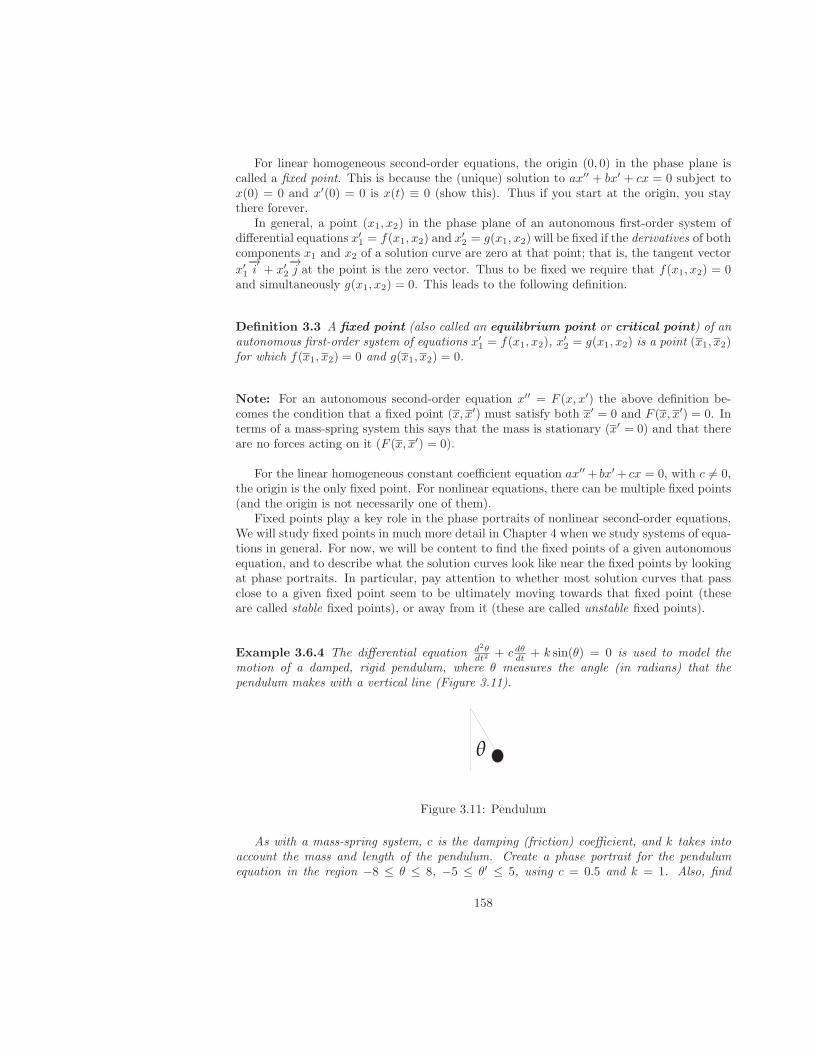
For linear homogeneous second-order equations, the origin (0, 0) in the phase plane iscalled a fixed point. This is because the (unique) solution to ax′′ + bx′ + cx = 0 subject tox(0) = 0 and x′(0) = 0 is x(t) ≡ 0 (show this). Thus if you start at the origin, you staythere forever.
In general, a point (x1, x2) in the phase plane of an autonomous first-order system ofdifferential equations x′
1 = f(x1, x2) and x′2 = g(x1, x2) will be fixed if the derivatives of both
components x1 and x2 of a solution curve are zero at that point; that is, the tangent vector
x′1
−→i + x′
2
−→j at the point is the zero vector. Thus to be fixed we require that f(x1, x2) = 0
and simultaneously g(x1, x2) = 0. This leads to the following definition.
Definition 3.3 A fixed point (also called an equilibrium point or critical point) of anautonomous first-order system of equations x′
1 = f(x1, x2), x′2 = g(x1, x2) is a point (x1, x2)
for which f(x1, x2) = 0 and g(x1, x2) = 0.
Note: For an autonomous second-order equation x′′ = F (x, x′) the above definition be-comes the condition that a fixed point (x, x′) must satisfy both x′ = 0 and F (x, x′) = 0. Interms of a mass-spring system this says that the mass is stationary (x′ = 0) and that thereare no forces acting on it (F (x, x′) = 0).
For the linear homogeneous constant coefficient equation ax′′+ bx′+ cx = 0, with c 6= 0,the origin is the only fixed point. For nonlinear equations, there can be multiple fixed points(and the origin is not necessarily one of them).
Fixed points play a key role in the phase portraits of nonlinear second-order equations.We will study fixed points in much more detail in Chapter 4 when we study systems of equa-tions in general. For now, we will be content to find the fixed points of a given autonomousequation, and to describe what the solution curves look like near the fixed points by lookingat phase portraits. In particular, pay attention to whether most solution curves that passclose to a given fixed point seem to be ultimately moving towards that fixed point (theseare called stable fixed points), or away from it (these are called unstable fixed points).
Example 3.6.4 The differential equation d2θdt2 + cdθdt + k sin(θ) = 0 is used to model the
motion of a damped, rigid pendulum, where θ measures the angle (in radians) that thependulum makes with a vertical line (Figure 3.11).
Figure 3.11: Pendulum
As with a mass-spring system, c is the damping (friction) coefficient, and k takes intoaccount the mass and length of the pendulum. Create a phase portrait for the pendulumequation in the region −8 ≤ θ ≤ 8, −5 ≤ θ′ ≤ 5, using c = 0.5 and k = 1. Also, find
158
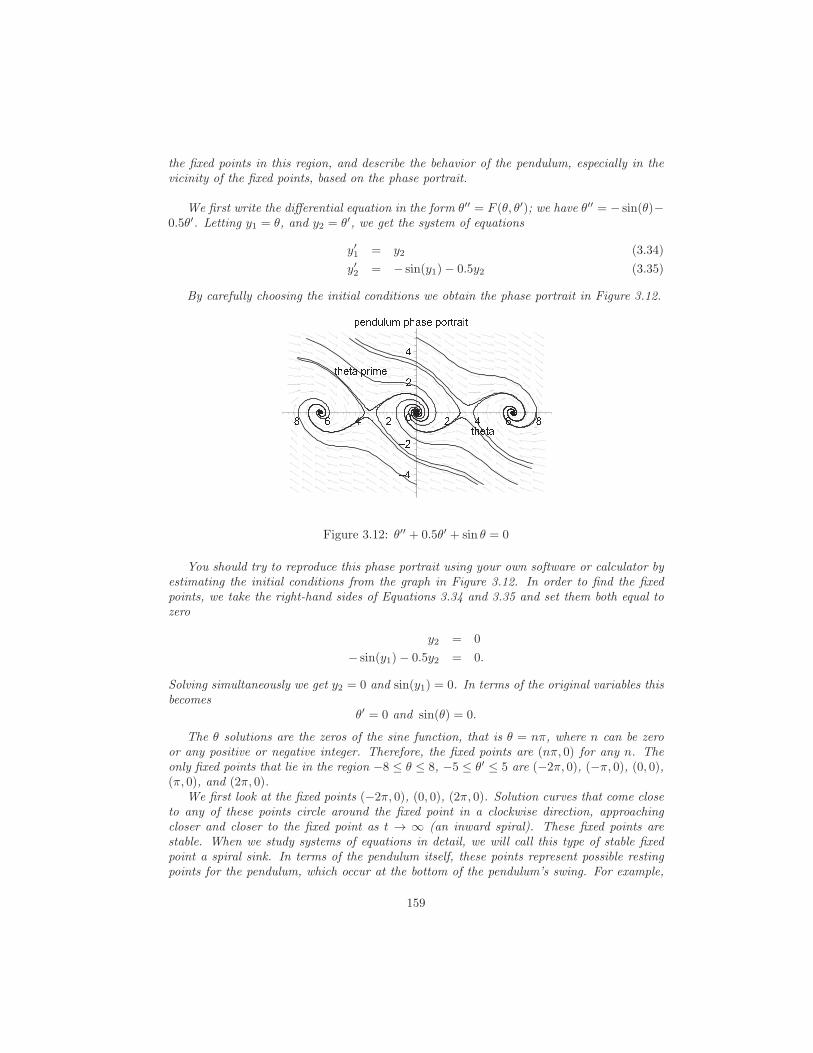
the fixed points in this region, and describe the behavior of the pendulum, especially in thevicinity of the fixed points, based on the phase portrait.
We first write the differential equation in the form θ′′ = F (θ, θ′); we have θ′′ = − sin(θ)−0.5θ′. Letting y1 = θ, and y2 = θ′, we get the system of equations
y′1 = y2 (3.34)
y′2 = − sin(y1)− 0.5y2 (3.35)
By carefully choosing the initial conditions we obtain the phase portrait in Figure 3.12.x y z { | } | ~ x � � � y x � � � � � � �� �� � ���� � y � � x � � ~ y� � � � � � � � � � � �� � y � �
Figure 3.12: θ′′ + 0.5θ′ + sin θ = 0
You should try to reproduce this phase portrait using your own software or calculator byestimating the initial conditions from the graph in Figure 3.12. In order to find the fixedpoints, we take the right-hand sides of Equations 3.34 and 3.35 and set them both equal tozero
y2 = 0
− sin(y1)− 0.5y2 = 0.
Solving simultaneously we get y2 = 0 and sin(y1) = 0. In terms of the original variables thisbecomes
θ′ = 0 and sin(θ) = 0.
The θ solutions are the zeros of the sine function, that is θ = nπ, where n can be zeroor any positive or negative integer. Therefore, the fixed points are (nπ, 0) for any n. Theonly fixed points that lie in the region −8 ≤ θ ≤ 8, −5 ≤ θ′ ≤ 5 are (−2π, 0), (−π, 0), (0, 0),(π, 0), and (2π, 0).
We first look at the fixed points (−2π, 0), (0, 0), (2π, 0). Solution curves that come closeto any of these points circle around the fixed point in a clockwise direction, approachingcloser and closer to the fixed point as t → ∞ (an inward spiral). These fixed points arestable. When we study systems of equations in detail, we will call this type of stable fixedpoint a spiral sink. In terms of the pendulum itself, these points represent possible restingpoints for the pendulum, which occur at the bottom of the pendulum’s swing. For example,
159
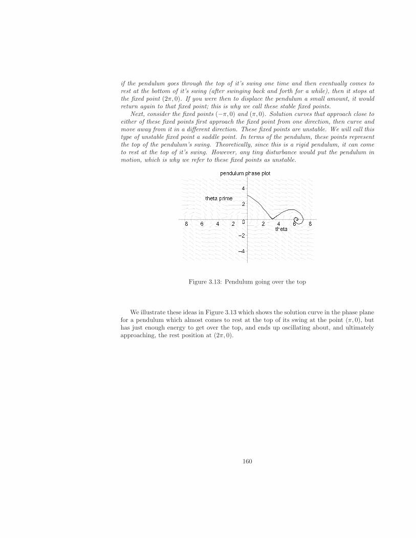
if the pendulum goes through the top of it’s swing one time and then eventually comes torest at the bottom of it’s swing (after swinging back and forth for a while), then it stops atthe fixed point (2π, 0). If you were then to displace the pendulum a small amount, it wouldreturn again to that fixed point; this is why we call these stable fixed points.
Next, consider the fixed points (−π, 0) and (π, 0). Solution curves that approach close toeither of these fixed points first approach the fixed point from one direction, then curve andmove away from it in a different direction. These fixed points are unstable. We will call thistype of unstable fixed point a saddle point. In terms of the pendulum, these points representthe top of the pendulum’s swing. Theoretically, since this is a rigid pendulum, it can cometo rest at the top of it’s swing. However, any tiny disturbance would put the pendulum inmotion, which is why we refer to these fixed points as unstable.x y z { | } | ~ x � � � y x } � �
� �� � ���� � y � � x � � ~ y� � � � � � � � � � � �� � y � �Figure 3.13: Pendulum going over the top
We illustrate these ideas in Figure 3.13 which shows the solution curve in the phase planefor a pendulum which almost comes to rest at the top of its swing at the point (π, 0), buthas just enough energy to get over the top, and ends up oscillating about, and ultimatelyapproaching, the rest position at (2π, 0).
160
Exercises 3.6
For problems 1-4, solve each initial value problem, and display the exact solution in thephase plane and also as x(t) and x′(t) time plots. Use 0 ≤ t ≤ 5, and choose appropriateintervals for x and x′. Give an interpretation of each equation and its solution as a mass-spring system.
1. x′′ + 7x′ + 12x = 0, x(0) = 0, x′(0) = 10 .
2. x′′ + 7x′ + 12x = 3 cos 3t, x(0) = 0, x′(0) = 10 .
3. x′′ + 2x′ + 17x = 0, x(0) = 5, x′(0) = 0 .
4. x′′ + 2x′ + 17x = 20 sin 10t, x(0) = 5, x′(0) = 0 .
For problems 5-8, redo problems 1-4, but this time generate the plots (phase plot andtwo time plots) using a numerical method as in Example 3.6.3 (do not create an entirephase portrait, just the plots for the one solution curve corresponding to the IVP).State which numerical method you are using, and any other relevant settings such asstep size or error tolerance. Use whatever technology you have available, or you canuse the applet for graphing and calculating numerical solutions for systems of equationsat uhaweb.hartford.edu/rdecker/MathletToolkit/SystemsBook.htm.
5. Use the IVP from problem 1.
6. Use the IVP from problem 2.
7. Use the IVP from problem 3.
8. Use the IVP from problem 4.
For problems 9-12, sketch a direction field for each autonomous second-order differ-ential equation by hand, using a 3 by 3 array of vectors in the region −1 ≤ x ≤ 1,−1 ≤ x′ ≤ 1 as in Example 3.6.2.
9. Use the DE from problem 1.
10. Use the DE from problem 3.
11. x′′ − 5x′ + 6x = 0.
12. x′′ + x′ − 6x = 0.
For problems 13-16 create a phase portrait for the given linear autonomous equationin the region −5 ≤ x ≤ 5, −20 ≤ x′ ≤ 20. It should include a direction field andenough well-chosen solution curves to give a complete picture of the equation on thespecified region. From the picture, determine whether the fixed point at the origin isstable or unstable. Use whatever technology you have available, or you can use theapplet for graphing and calculating numerical solutions for systems of equations atuhaweb.hartford.edu/rdecker/MathletToolkit/SystemsBook.htm.
13. Use the DE from problem 1.
14. Use the DE from problem 3.
161
15. x′′ − 5x′ + 6x = 0.
16. x′′ + x′ − 6x = 0.
For problems 17-18 create a phase portrait for the given nonlinear autonomous equationin the given region. Also find any fixed points that occur in that region. Your phaseportrait should include a direction field and enough well-chosen solution curves togive a complete picture of the equation on the specified region, especially near thefixed points. From the picture, determine which fixed points are stable and which areunstable. Use whatever technology you have available, or you can use the applet forgraphing and calculating numerical solutions for systems of equations at
uhaweb.hartford.edu/rdecker/MathletToolkit/SystemsBook.htm
17. y′′ +2y′ − 17(4 ∗ y− y3) = 0 on −5 ≤ y ≤ 5, −20 ≤ y′ ≤ 20 (this equation can be usedas a model of a mass-spring system with a repelling force at the origin - explain why,using your phase portrait).
18. d2θdt2 + 2dθ
dt + sin θ = 0 on −7 ≤ θ ≤ 7, −1 ≤ θ′ ≤ 1 (note that this is the pendu-lum equation from Example 3.6.4 - relate the behavior of the pendulum to your phaseportrait).
Lab 2: Nonlinear forces and the Duffing equation
Introduction
We have spent a great deal of time studying the linear mass-spring equationmx′′+cx′+kx =f(t), where x represents the displacement from equilibrium of an object of massm suspendedfrom a linear spring with spring constant k and damping constant c. The independentvariable is t which represents the time. The forcing function f(t) (when it is not zero)has often been assumed to be of the form a cos(ωt) or a sin(ωt). The term kx representsthe force, as a function of x, for a linear spring; if we replace that term with a nonlinearfunction of x we get a nonlinear force on the mass. For some nonlinear forces this can stillbe considered to be a mass-spring system (see the investigation of hard and soft springsbelow), but for other forces a different physical model is needed.
One of the most-studied, and simplest, examples of a nonlinear mass-spring equation isthe Duffing equation
mx′′ + cx′ + kx+ bx3 = f(t).
Here the force on the mass is given by the cubic function kx+bx3. When written as a systemof first-order differential equations, using the usual substitution y = x′, we get x′ = y andy′ = −cy− kx− bx3 + f(t). Two good websites that give an introduction to this very inter-esting equation are http://www.scholarpedia.org/article/Duffing\_oscillator andhttp://mathworld.wolfram.com/DuffingDifferentialEquation.html (the letters usedfor the various parameters are not completely standard, so be careful when applying theinformation from those websites to this project).
Clearly the only difference between the Duffing equation and the standard mass-springequation is the replacement of the linear term kx by the nonlinear term kx+bx3. This termtherefore describes the force on the mass when it is displaced x units from its equilibriumposition. Surprisingly, this simple looking term can describe a number of different physical
162
systems, depending on the choice of parameters k and b. Note on the direction of the force:For a linear mass-spring system, the derivation of the equation mx′′ + cx′ + kx = f(t)comes from Newton’s second law, which says that the mass of an object multiplied by itsacceleration is equal to the sum of all forces acting on the object. For the mass-springsystem this becomes mx′′ = −cx′ − kx+ f(t). The negative sign on the kx term is there sothat when the spring is extended in the direction of positive x, the force acts in the oppositedirection in order to restore the spring to its rest position (a similar argument works for thedamping force cx′). Thus keep in mind for activities below, that when you graph the forcekx+ bx3, one expects that for a spring the graph would be positive (above the x-axis) whenx is positive, and negative (below the x-axis) when x is negative.
Hard and soft springs and the Duffing equation
First we want to understand what is meant by the terms “soft spring” and “hard spring”.
1. Graph the linear and nonlinear spring-force functions kx and kx + bx3 together fork = 1 and b varying from −3 to 5. First compare the two graphs near the origin (forthis choose a graph window that is something like −0.1 to 0.1 in both the horizontaland vertical directions). Is there much difference between the two graphs? Whatdoes this imply about the nonlinear model for small oscillations (small displacementsx from the origin)? When the displacement x is sufficiently small, we say that thenonlinear spring is in the linear range.
2. Next compare the two graphs further from the origin (say with a graph window −1to 1 in both directions). Again, let b vary between −3 and 5. In particular noticewhether the graph of kx + bx3 is above (stronger force) or below (weaker force) thegraph of kx. For which values of b is the force of the spring in the nonlinear modelgreater than that of the linear model for positive x? For which values of b is the forceless than for the linear model for positive x? Explain why the nonlinear spring is calleda soft spring when b < 0 and a hard spring when b > 0. Are these terms appropriatefor small oscillations also (remember what you observed in part 1)?
3. Investigate the question “For what range of x values is the force equation kx + bx3
physically realistic?” Consider both hard and soft springs, using the b values andwindow setting from part 2. In particular, for any sensible spring the force shouldpull the spring back towards the equilibrium position for any amount of displacementx; if the graph of the force goes negative, then the spring is pushing the mass awayfrom the equilibrium position (a repelling force), which a spring would never do. Amore subtle consideration would be that as x gets larger, the force should get larger.Otherwise, the spring would feel “tight” for small x and “loose” for large x, sort oflike a piece of taffy. The problem is that once taffy is stretched out, it does not snapback to its original state as a spring does. Find the values of x for which the springbecomes somewhat physically unrealistic (the “taffy” spring) and which are totallyimpossible for a real spring (the repelling spring) in terms of the constants k and b.Note: this does not mean that soft springs in general are not possible for large x, onlythat the Duffing equation must be restricted to a certain range of x values in orderfor it to be used as a model of a soft spring.
Now that we understand how the term kx + bx3 works as a model for soft and hardsprings, we investigate the behavior of the entire mass-spring system (as modelled by
163
the Duffing equation) for soft and hard springs. We will restrict our discussion to thecase when the displacements are large enough that the nonlinear spring is no longerin the linear range (see 1 above), and to the case when there is no damping (c = 0),and no forcing function (f(t) = 0).
4. Obtain graphs of the solution curves to mx′′ + cx′ + kx + bx3 = 0 for m = 1, c = 0,k = 1, with the initial conditions x(0) = 0.5 and x′(0) = 0, and let b increase slowlyfrom −3 to 5. Look at both a phase plot (plotting the spring-force function kx+bx3 ontop of the phase plot helps relate this exercise with the previous ones) and a time plot.Good ranges for the phase plot are −1 to 1 in the both directions, and for the timeplot 0 to 20 in the horizontal (t) direction and −1 to 1 in the vertical (x) direction.Time plots reveal the period/frequency of the oscillations. How does the softness orhardness of the spring (the value of b) affect the period and frequency? Note anythingelse of interest that you observe in either the phase or time plots.
5. Using the same graph windows as in part 3, fix b = −2 (soft spring) and let the initialposition x(0) vary (keeping x′(0) = 0). How does the period/frequency depend onx(0)? For what initial positions x(0) is the response of the spring physically unrealistic(see part 3 from above)? Repeat for b = 5 (hard spring) and answer the same questions.How does the period/frequency depend on x(0) for a linear spring (think about whatit means for a linear spring to have a “natural” frequency)? Do nonlinear springs havea natural frequency? Explain.
6. As noted in the introduction, the corresponding first-order system for the Duffingequation is x′ = y, y′ = −cy − kx − bx3 (since we are currently assuming thatf(t) = 0). Find the fixed points for the system. Now, for b = −2 (soft spring) create aphase portrait (many solution curves) and/or a direction field in order to observe theglobal behavior of the system. Again it is helpful to graph the spring force kx + bx3
on the same set of axes as the phase portrait (the intersections of that curve with thehorizontal axis are the fixed points - show why). Carefully describe what the variouspossible solution curves represent in terms of the spring. In your discussion includethe solution curves that correspond to physically non-realistic springs as discussed inpart 3. Are the fixed points stable or unstable based on the phase portrait? Repeatfor b = 5 (hard spring) and answer the same questions.
Beams and magnets and the Duffing equation
Hard and soft springs correspond to what is called a single well potential: this means thatthere is a single stable fixed point, as we saw in part 6 of “Hard and soft springs”. Here wewill see that the Duffing equation mx′′+cx′+kx+bx3 = f(t) can be used to model systemsthat have two stable fixed points, with an unstable fixed point between them (a double wellpotential). There are a number of ways of creating such a system. See the first websitegiven in the introduction for an example, where a thin flexible metal beam is suspendedbetween two magnets (the beam is stable when it is bent towards one magnet or the other,but unstable when it is in the middle).
The parameters m and k will no longer have the exact same interpretation as for amass-spring system, although m will be related to (but not equal to) the mass of the beam.The c parameter can still be interpreted as a damping constant.
164
1. We first investigate the beam-magnet force given by the term kx+ bx3. When appliedto the beam-magnet system, x represents the displacement of the tip of the beam. Ofcourse, this is the same function as for the hard and soft springs, but this time weassume that k is negative. Graph kx + bx3 in a graph window with both horizontaland vertical axes running from −1 to 1. Set k = −1. Let b vary between −3 and 5.For what values of b does this force function represent a double well potential (a beam-magnet system)? For b values which do not correspond to a double well potential, canyou think of a real system which would act like this?
2. Again for k = −1, choose a typical b value that represents a double well based onyour investigation in part 1. With this b value create a phase plot and a time plotfor the unforced, undamped Duffing equation x′′ + kx+ bx3 = 0 (with m = 1). Startwith x(0) = 0.5 and x′(0) = 0, then vary x(0) to see what type of solution curves arepossible for these parameter values. Do all solution curves correspond to oscillationsof some type? Explain how the solution curves correspond to the motion of the tip ofthe beam in the beam-magnet system (x is as in part 1). Discuss both the phase plotand the time plot.
3. For k = −1 and the same b value and equation as in part 2, create a phase portrait(several solution curves). Adding a direction field can help also. Do not include timeplots, as they tend to get “tangled” when many are plotted at once. Now slowlyincrease k and continue until it reaches k = 1. At this point you should be back tothe hard spring of the “Hard and soft springs” investigation. Explain what happenedto the various fixed points and their stability as k changed. Also relate what happensto the beam-magnet system. Can you relate the value of k to any property of thebeam-magnet system? Explain.
Beats, resonance and chaos in the Duffing equation
Recall that for the undamped linear mass-spring equation mx′′ + kx = f(t) one observesbeats when the forcing function is periodic (we will assume the form a sin(ωt)) and the
natural frequency (given by
√k/m
2π ) is close to the driving frequency (given by ω2π ). Res-
onance occurs when the two frequencies are exactly equal. Do we get similar phenomenawith nonlinear systems?
1. Demonstrate with time plots how beats turn into resonance and back to beats in thelinear, undamped mass-spring equation mx′′ + kx = a sin(ωt). Use m = 1, k = 1,a = 1, x(0) = x′(0) = 0 and let ω vary slowly between 0.5 and 1.5. Resonance occursat ω = 1 (explain why). Describe both in words and pictures what happens. Supposeyou are observing a mechanical system, such as the vibrations of an airplane wing,and you detect beats. As time passes, the beats are getting farther and farther apartin time, so you think things are getting better. Are they?
2. One can observe beats in nonlinear systems as well. Recall that from the “Beams andmagnets” activity above, when k is negative the Duffing equation can be thought of as amodel for a beam-magnet system. For the Duffing equation mx′′+kx+bx3 = a sin(ωt)with k = −1, b = 1, a = 0.07, x(0) = 1, x′(0) = 0, let ω vary slowly between 1 and2. Again, describe what happens in terms of beats. Does resonance occur this time?What does occur? Describe as best you can, both in mathematical terms (include a
165

discussion of fixed points) and in terms of the beam-magnet system. Relate this tothe information you found at the websites listed in the introduction.
166
Linear Algebra Interlude
Linear algebra is a branch of mathematics that can be used to solve problems that involvea large number of variables and a large number of equations. The important requirementfor linear algebra to be helpful is that the variables must appear in a linear way in theequations. When that is the case, linear algebra techniques can be used to solve bothalgebraic equations and differential equations.
Suppose x, y, z are variables that represent the x, y, z displacements of one end of a beamin a large structure. In static equilibrium, these variable may satisfy a set of equations suchas
2x+ 3y + 5z = 10x+ y + 7z = 123x+ 7y + 8z = 5
Notice that the variables all appear in a linear way (multiplied by a constant, but notraised to a power, no exponential or trig functions of variables, and so on). These equationscan then be solved using linear algebra for x, y, and z. In a real structure, there may bethousands of variables and equations.
We can also describe and solve systems of linear DE’s. For the structure described onthe previous slide, if the end of the beam is not in static equilibrium, then we may needdifferential equations to describe its motion. We might get a system such as
x′ = 2x+ 3y + 5zy′ = x+ y + 7zz′ = 3x+ 7y + 8z
Again, for linear algebra to apply, the system must be linear in all dependent variables. Asbefore, there may be many more than three equations and three dependent variables in areal system (structure, circuit, ecosystem).
A. Matrices, Vectors, Scalars
A matrix is a rectangular array of numbers, usually enclosed by brackets. Generally we useuppercase letters to represent matrices. Here is a matrix with 2 rows and 3 columns:
A =
[0 1 −23 −4 5
]
We list the number of rows first then the number of columns when describing a matrix.Thus the matrix A above is referred to as a 2 by 3, or 2× 3 matrix. Shortly we will see howmatrices are used to describe large systems of linear algebraic or differential equations.
167
A vector is just a matrix with one column or one row. We will normally work withvectors that consist of just one column, called column vectors. A row vector would havejust one row. We use lower case letters for vectors such as
b =
[1−2
]
A scalar is a 1 by 1 matrix, that is, just a single number. Use lower case for scalars,such as c = 5.
Matrix algebra
Much of the power of using matrices to describe linear systems, is that you can manipu-late them using algebraic operations that mimic the algebraic operations of numbers andvariables that you learned in high school.
Matrix addition
Matrices of the same size can be added, term by term. Thus a 2×2 matrix can be added toanother 2× 2 matrix; just add corresponding entries. If the two matrices are not the samesize, matrix addition is not defined. For example if
A =
[1 23 4
]
and B =
[−1 13 2
]
(3.36)
then
A+B =
[1− 1 2 + 13 + 3 4 + 2
]
=
[0 36 6
]
Scalar multiplication
A matrix can be multiplied by a scalar; just multiply each element of the matrix by thescalar. If we define the scalar c = 2, with A defined above, then
cA =
[2(1) 2(2)2(3) 2(4)
]
=
[2 46 8
]
Matrix multiplication
In certain cases, matrices can be multiplied. First we define the product of a column vectorand a row vector, where both are the same length. If c is a row vector and d is a column vectorof the same length, the product cd is a scalar that results from multiplying correspondingentries (first entry of c times first entry of d, then second entry of c times second entry ofd, etc.), then adding the results. Thus for the vectors
c =[1 3
]and d =
[−22
]
we get
cd = 1(−2) + 3(2) = 4
168
To multiply matrix A times matrix B, multiply each row of A times each column of B.The row i column j entry of AB results from multiplying row i of A times column j ofB. For example, to get the entry in row 2 and column 3 of AB multiply row 2 of A timescolumn 3 of B. Matrix multiplication is defined only if the number of columns of A is equalto the number rows of B. Thus using A and B from Equation (3.36) we get
AB =
[(row 1)(col 1) (row 1)(col 2)(row 2)(col 1) (row 2)(col 2)
]
We mention some important properties of matrix multiplication
• If A is an i× j matrix and B is a k× l matrix, then AB is defined if and only if j = k(that is, if the number columns of A is the same as the number of rows of B).
• If A is i× j and B is j × k then AB is defined and is an i× k matrix.
• In general AB 6= BA even when both are defined.
Example 3.6.5 Let A =
[0 2 −31 3 2
]
, B =
[1 −12 0
]
, c =
[2−1
]
, d = −2. Find A + B,
B + c, B +B, AB, BA, Ac, Bc, dA, and dc. If given operation is not defined, say so.
Solution. A + B is not defined. B + c is not defined. B + B =
[2 −24 0
]
, AB is not
defined. BA =
[−1 −1 −50 4 −6
]
. Ac is not defined. Bc =
[34
]
. dA =
[0 −4 6−2 −6 −4
]
,
dc =
[−42
]
.
Special matrices, trace, determinant
Two special matrices of importance are the zero matrix and the identity matrix. The zeromatrix is denoted 0 and is a matrix of all zeros; it can be any size. The size of the matrix
can be inferred from context. For example if A =
[1 2−1 3
]
then in the equation A+ 0 = A
we mean 0 =
[0 00 0
]
.
The identity matrix is a square matrix (same number of rows as columns), which consistsof all ones and zeros, in the following arrangement. The elements that appear in row i,column i, for any i, are ones, and all other elements are zeros. Thus, row 2, column 2 has a
one, but row 1, column 2 has a zero. For example the 2× 2 identity is I =
[1 00 1
]
and the
3× 3 identity is I =
1 0 00 1 00 0 1
.
Note that A+0 = 0+A = 0 and AI = IA = A for any matrix A. Thus the zero matrixacts like the number 0 does for real numbers and the identity matix acts like the number 1does for real numbers.
The determinant and the trace are defined for square matrices ( n × n matrices of any
size). The determinant of a 2×2 matrix A =
[a bc d
]
is defined to be det(A) = ad− bc. The
169
determinant is also defined for larger square matrices; see the exercises. For systems largerthan 2× 2 we will mostly rely on software to do our calculations for us.
The trace of a square matrix is defined to be the sum of the diagonal elements (theelements in row 1, column 1 and row 2, column 2, and so on). Thus for a 2 × 2 matrix
A =
[a bc d
]
we have trace(A) = a+ d.
Systems of algebraic equations in matrix form
Consider the system of algebraic equations
2x1 − x2 = 1x1 + x2 = 3
(3.37)
This system is linear; also there are two equations and two unkowns. It is systems of thistype that we will be interested in - systems of n linear equations with n unknowns. We canput this system into matrix form as follows. Define
A =
[2 −11 1
]
, x =
[x1
x2
]
and b =
[13
]
Using the definition of matrix multiplication we get Ax =
[2x1 − x2
x1 + x2
]
. Since two matrices
are equal if and only if all corresponding entries are equal, Equations (3.37) becomes
Ax = b
in matrix form.We will need to use one of the major theorems in linear algebra. It states that the system
Ax = b has either one solution, no solutions or infinitely many solutions for the unknownvector x. Furthermore, if A is a square matrix, then there is exactly one solution (a uniquesolution) if and only if det(A) 6= 0.
Example 3.6.6 For each system below, determine whether or not there is a unique solution.If there is a unique solution find it; if not find 3 solutions.
a)2x1 + 3x2 = 0x1 − x2 = 0
b)2x1 + 4x2 = 0x1 + 2x2 = 0
Solution.
a) We have A =
[2 31 −1
]
and b =
[00
]
so that det(A) = 2(−1) − 1(3) = −5 and hence
the solution is unique. By inspection,
[00
]
(that is, x1 = 0 and x2 = 0 ) is the unique
solution. When b =
[00
]
the zero vector will always be a solution (do you see why?).
b) We have A =
[2 41 2
]
and b =
[00
]
so that det(A) = 2(2) − 1(4) = 0 and hence there
is not a unique solution. We will again have the solution
[00
]
.
To find two other solutions, we can solve each of the equations for one of the vari-ables, say x1. We get x1 = −2x2 for both the first and second equation. This means we
170
can choose anything we want for one of the variables, and then calculate the other. It alsomeans there are infinitely many solutions. If we chooe x2 = 1 we get x1 = −2 and if we
choose x2 = 2 we get x1 = −4. In vector form the two other solutions are
[−21
]
and
[−42
]
.
Systems of DE’s in matrix form
We can also write systems of differential equations in matrix form. First we must define
what it means to take the derivative of a vector function. If x(t) =
x1(t)x2(t)...
xn(t)
then we define
x′(t) =
x′1(t)
x′2(t)...
x′n(t)
, that is, we differentiate terms by term.
Example 3.6.7 Write the DE system
x′1 = 2x1 − x2
x′2 = x1 + x2
in matrix form.Solution. Define
A =
[2 −11 1
]
and X =
[x1
x2
]
Then AX =
[2x1 − x2
x1 + x2
]
and X ′ =
[x′1
x′2
]
so the DE system above becomes
X ′ = AX
Exercises 3.7 Given the following matrices
A =
(2 1−3 4
)
, B =
(−1 21 3
)
, C =
(0 1 2−3 −4 1
)
, D =
(0 1−3 −4
)
;
Compute each expression 1 - 6 below, if it is defined; otherwise state why it is not defined.
1. A+B
2. 2A+ (−3)B
3. C(A+B)
4. (A+B)C
5. ABC
6. A− 2I
7. 2A+ 0
171
8. Show that AB 6= BA.
9. Find the trace and determinant of the matrix A.
10. Find the trace and determinant of the matrix B.
For each of the following algebraic systems of equations, identify the matrix A and thevector b that corresponds to the matrix equation Ax = b.
11. x1 − x2 = 2, 3x1 − 4x2 = 5
12. −x1 − 3x2 = 0, −2x2 = 4
For each of the following systems of differential equations, identify the matrix A thatcorresponds to the matrix equation x′ = Ax.
13. x′1 = x2, x
′2 = x1 − x2
14. x′1 = −x1 + 3x2, x
′2 = 2x1 − 4x2
B. Eigenvalues and Eigenvectors
Given a square matrix A (for this text, we mostly work with 2×2 matrices), the eigenvalue-eigenvector problem is to find scalars r and vectors u (we want non-zero u) for which
Au = ru (3.38)
The scalars are the eigenvalues and the vectors are the eigenvectors. Using a little matrixalgebra Equation (3.38) can be written as Au = rIu and then Au− rIu = 0 and finally
(A− rI)u = 0 (3.39)
We will call equation Equation (3.39) the eigenvector equation.One vector u that always solves Equation (3.39) is the zero vector u = 0. From the
previous section we know that Equation (3.39) must have either one solution, no solutions,or infinitely many solutions. Thus for there to be any non-zero u that are solutions, theremust be infinitely many such solutions, and again from the previous section, this requiresthat
det(A− rI) = 0 (3.40)
We will call Equation (3.40) the eigenvalue equation. For each eigenvalue r that you getfrom Equation (3.40), use Equation (3.39) (A− rI)u = 0 to get a corresponding eigenvectoru. You should end up with pairs (r1, u1), (r2, u2) and so on (for 2× 2 matrices you get twopairs).
NOTE: If r1 = r2 we have a repeated eigenvalue. In this case there can be either one ortwo (linearly independent) eigenvectors.
Example 3.6.8 Let A =
[1 41 1
]
. Find the eigenvlue/eigenvector pairs.
Solution. The Equation (3.40), the eigenvalue equation det(A− rI) = 0,
becomes det
([1 41 1
]
− r
[1 00 1
])
= det
([1− r 41 1− r
])
172

= (1− r)2 − 4 = 0. The solutions to this quadratic are r1 = −1 and r2 = 3; they are theeigenvalues.
For the eigenvectors we use Equation (3.39), the eigenvector equation (A−rI)U = 0.
By letting U =
[x1
x2
]
, this becomes
([1 −41 1
]
− r
[1 00 1
])[x1
x2
]
=
[00
]
or
[1− r 41 1− r
] [x1
x2
]
=
[00
]
This results in two equations (1 − r)x1 + 4x2 = 0 and x1 + (1 − r)x2 = 0. For theeigenvalue r1 = −1 these equations become 2x1 + 4x2 = 0 and x1 + 2x2 = 0; both equationsgive x1 = −2x2. This means that we only need one of the two equations, and we can chooseany value we want for x2; for example if x2 = 1 then x1 = −2x2 = −2 and the eigenvector
is U1 =
[−21
]
.
For the eigenvalue r1 = 3 the eigenvector equations (1 − r)x1 + 4x2 = 0 and x1 +(1 − r)x2 = 0 become -2x1 + 4x2 = 0 and x1 − 2x2 = 0; both equations give x1 = 2x2.Again we only need one of the two equations, and we can choose any value we want for x2;
if x2 = 1 then x1 = 2x2 = 2 and the eigenvector is U2 =
[21
]
.
We now have our two eigenvalue-eigenvector pairs. They are
(
−1,
[−21
])
and(
3,
[21
])
Properties of eigenvalues and eigenvectors.
1. Any multiple of an eigenvector is the same eigenvector. For example x =
[12
]
is the
same eigenvector as x =
[0.447 210.894 43
]
. This is because if Au = λu then Acu = λcu
(multiply both sides by the scalar c) which shows that cu is an eigenvector.The secondform above is a unit vector, and is how the TI gives you eigenvectors.
2. Eigenvalues and eigenvectors can be real or complex. There are three cases: two realeigenvalues, one real eigenvalue, two complex eigenvalues (sound familiar?). On theTI89 make sure that under MODE the Complex Format is set to Rectangular.
3. When the eigenvalues are complex they come in complex conjugate pairs r = α ± β.When this happens, the eigenvectors also come in complex conjugate pairs U = W±iV .See the next example.
Eigenvalues and eigenvectors on the TI89
• Store a matrix in a variable such as a using [1, 2; 3,−1] → a.
• Use math-matrix-eigVl for eigenvalues and math-matrix-eigVc for eigenvectors.
• The first column of the eigenvector matrix is the eigenvector that corresponds to thefirst eigenvalue (second column corresponds to second eigenvalue).
173
Example 3.6.9 Let A =
[1 −41 1
]
.The eigenvalues and eigenvectors are complex; find α,
β, W , and V .Solution. After storing the matrix and giving the eigenvalue command, the TI89 gives
us r1 = 1 + 2i and r2 = 1 − 2i. Thus α = 1 and β = 2. The eigenvector command gives[
.894427191 .894427191−.4472135955i .4472135955i
]
. The first eigenvector is
[.894427191 + 0i0− .4472135955i
]
, which can be
expanded into its real and imaginery parts as
[.894427191
0
]
+
[0
−.4472135955
]
i. This means
that W =
[.894427191
0
]
and V =
[0
−.4472135955
]
.
The result can be simplifed by multiplying the complex eigenvector
[.894427191
−.4472135955i
]
by 1.4472135955 to get the complex eigenvector
[2−i
]
which expands to
[20
]
+
[0−1
]
i. Then one
can use W =
[20
]
and V =
[0−1
]
.
Three things to note: 1) both W and V are real vectors, 2) neither W nor V areeigenvectors, and 3) only the first complex eigenvector is needed (the second one would leadto the same W and V ).
Exercises 3.8 For each of the matrices 1 - 6 below, find the eigenvalues. Find an eigen-vector corresponding to each eigenvalue. In each case, do this first by hand and then usetechnology (TI-86, TI-89, Maple, etc.). Explain any differences.
1. A =
(−2 21 −3
)
2. B =
(2 10 −3
)
3. C =
(−4 2−2 0
)
4. D =
(1 −44 −7
)
5. E =
(1 3−3 1
)
6. F =
(2 8−1 −2
)
174
Chapter 4
Systems of First-order
Differential Equations
4.1 Explicit Solutions of Constant-coefficient Linear Sys-
tems
From the second linear algebra section we know that a system of DE’s x′1 = ax1 + bx2,
y′ = cx1 + dx2 can be written in matrix form as[x1
x2
]′
=
[a bc d
] [x1
x2
]
or X ′ = AX where X =
[x1
x2
]
and A =
[a bc d
]
. To solve X ′ = AX
we assume a solution of the form X(t) = ertU where U is a vector of constants U =[u1
u2
]
.This leads to X ′ = rertU so that the equation X ′ = AX becomes rertU = AertU . We
then divide out the ert and rearrange to get AU = rU which is the eigenvalue-eigenvectorequation, Equation (3.38).
The General Solution
Recall that there are three cases for the eigenvalues: two real eigenvalues, two complexeigenvalues, and one real eigenvalue (also referred to as repeated eigenvalues). If we havetwo distinct eigenvalues, then we get two (linearly independent) solutions X1 = er1tU1 andX2 = er2tU2. We can then take a linear combination C1X1+C1X2 for the general solution,similar to when we solved second order linear equations.
Thus the general solution to X ′ = AX for the 2 real eigenvalues case is
X = C1er1tU1 + C2e
r2tU2 (Two real eigenvalues)
For the case of two complex eigenvalues, we again proceed in a manner similar to whatwe did in Chapter 3 for second order equations, and invoke the property of linear differentialequations (or systems) that the real and imaginary parts of a complex solution to a DE orDE system are real valued solutions. Given that ertu is a solution, write r = α + βi andu = U + V i to get ertu = eαt(cos(βt) + i sin(βt))(U + V i) = eαt(cos(βt)U − sin(βt)V +cos(βt)V i + sin(βt)Ui) so that the real and imaginary parts are eαt(cos(βt)U − sin(βt)V )and eαt(cos(βt)V + sin(βt)U).
175
Thus the general solution to X ′ = AX for the 2 complex eigenvalues case is
X = C1eαt(cos(βt)U−sin(βt)V )+C2e
αt(cos(βt)V +sin(βt)U) (Two complex eigenvalues)
where the eigenvalues are α± βi and the eigenvectors are U ± V i.
Example 4.1.1 Find the general solutions to each system of differential equations.a) x′ = x+ 2y, y′ = 8x+ yb) x′ = x+ 2y, y′ = −8x+ ySolution.
a) We have A =
[1 28 1
]
. The eigenvalues and corresponding eigenvectors (from the
TI89) are r1 = 5, r2 = −3 and U1 =
[0.4472140.894427
]
, and U2 =
[−0.4472140.894427
]
. Since a multiple
of an eigenvector is still an eigenvector, if we multiply each eigenvector by 10.447214 we get
U1 =
[12
]
and U2 =
[−12
]
which provide for a “nicer” solution. The general solution is now
X = C1e5t
[12
]
+ C2e−3t
[−12
]
=
[C1e
5t − C2e−3t
2C1e5t + 2C2e
−3t
]
In component form (using the original variables) we get
x1 = C1e5t − C2e
−3t and x2 = 2C1e5t + 2C2e
−3t
b) We have A =
[1 2−8 1
]
. The eigenvalues and corresponding eigenvectors (from the
TI89) are r1 = 1 + 4i, r2 = 1− 4i and U1 =
[−0.447214i0.894427
]
, and U2 =
[0.447214i0.894427
]
. Since a
multiple of an eigenvector is still an eigenvector, if we multiply each eigenvector by 10.447214
we get U1 =
[−i2
]
and U2 =
[i2
]
. Expanding the complex eigenvectors into their real and
imaginary parts we get U1 =
[0− 1i2 + 0i
]
=
[02
]
−[10
]
i and U2 =
[0 + 1i2 + 0i
]
=
[02
]
+
[10
]
i.
From the eigenvalues we have α = 1 and β = 4, and from the eigenvectors we have
U =
[02
]
and V =
[10
]
. Notice that we really only needed the first eigenvalue and first
eigenvector. Using the general solution from the two complex eigenvalue case we get
X = C1e−t
(
cos(4t)
[02
]
− sin(4t)
[10
])
+ C2e−t
(
cos(4t)
[10
]
+ sin(4t)
[02
])
We could also write this solution as
X =
[−C1e
−t sin(4t) + C2e−t cos(4t)
2C1e−t cos(4t) + 2C1e
−t sin(4t)
]
so that in component form we have
x1 = −C1e−t sin(4t) + C2e
−t cos(4t) and x2 = 2C1e−t cos(4t) + 2C1e
−t sin(4t)
For the case of one real eigenvalue (repeated eigenvalues) we need to come up with asecond linearly independent solution. We will not cover this case at this time.
176
Initial Conditions
We treat systems with initial conditions the same way we did first-order and second-orderequations: after the general solution is found, use the initial conditions to find the constantsin the general solution. We illustrate with an applied example.
Example 4.1.2 In Hawaii, feral chickens have taken over the island of Kauai (fact). Letus assume that in one particular field, the chickens only source of food is worms, and at themoment the chickens and worm populations are stable at a level of 30 chickens and 2000worms (we call these equilibrium population values). Now let x = the number of chickensabove equilibrium, and let y = the number of worms above equilibrium. Thus if x = 5and y = −100 that means there are 35 chickens and 1900 worms. Though the model for apredator-prey situation such as this is actually nonlinear, as long as the chicken and wormpopulations are near the equilibrium values, the following linear model works well
x′ = −0.12x− 12y, y′ = 0.006x
where time is measured in months. If x and y both start at zero, they stay at zero (recallthis means 30 chickens and 2000 worms). Do you see why?
Now assume that 5 chickens are kidnapped (chickennapped?). What will happen toboth populations in the future? Use the initial conditions x = −5 and y = 0 (correspondingto 25 chickens and 2000 worms). Predict the size of both populations 3 months later, and10 years later.
Solution. We can find the general solution to the system above, then use the initialconditions to determine the constants, and finally predict the future using t = 3 and t = 120.
The system can be written as X ′ = AX, where A =
[−0.12 −12
0 0.006
]
and X =[xy
]
. The eigenvalues are −0.06± 0.261 53i and the eigenvectors are
[−0.99975
0.005± 0.021789i
]
=[−0.999750.005
]
±[
00.021789
]
i.Thus we are in the complex case with α = −0.06, β = 0.26153,
U =
[−0.999750.005
]
, and V =
[0
0.021789
]
.The general solution, using the complex case equa-
tion (and rounding a bit), is
X = C1e−0.06t
(
cos(0.262t)
[−0.999750.005
]
− sin(0.262t)
[0
0.021789
])
(4.1)
+C2e−0.06t
(
cos(0.262t)
[0
0.021789
]
+ sin(0.262t)
[−0.999750.005
])
We now use the initial conditions x(0) = 25 and y(0) = 2000, or in vector form
X(0) =
[−50
]
.From Equation (4.1) we have X(0) = C1
[−0.999750.005
]
+ C2
[0
0.021789
]
=[
−0.99975C1
0.005C1 + 0.021789C2
]
. Setting the two expressions for X(0) equal, we get the two equa-
tions
−0.99975C1 = −5 and 0.005C1 + 0.021789C2 = 0
177
The solution to these equations is C1 = 5.001 3, C2 = −1.147 7. Substituting into Equation(4.1) we get
X = 5.001 3e−0.06t
(
cos(0.262t)
[−0.999750.005
]
− sin(0.262t)
[0
0.021789
])
−1.147 7e−0.06t
(
cos(0.262t)
[0
0.021789
]
+ sin(0.262t)
[−0.999750.005
])
which upon multiplying out (and rounding) gives the component equations
x = −5.0 (cos 0.2615t) e−0.06t + 1. 1471 (sin 0.2615t) e−0.06t
y = −0.1147 (sin 0.2615t) e−0.06t
Finally, substituting t = 3 and t = 120 into the above equations we get
x(3) = −2. 279y(3) = −0.068
andx(120) = −0.004y(120) = 0.000
accurate to three decimal places. However, since both x and y repesent the size of a popula-tion, we conclude that after 3 months x = −2 and y = 0, which means 30− 2 = 28 chickensand 2000 worms. After 10 years we are back to 30 chickens amd 2000 worms. Thus it ap-pears that if the number of chickens and worms is varied slightly from the equilibrium valuesof 30 chickens and 2000 worms, the two populations eventually return to the equilibriumvalues.
Exercises 4.1 Find solutions to each of the following systems, given in component form.If initial conditons are not given, find a general solution. Give the solution in both vectorform and component form (that is, give expressions for x(t) and y(t)).
1. x′ = y, y′ = x.
2. x′ = −y, y′ = x.
3. x′ = 2x− y, y′ = y
4. x′ = −x, y′ = x, x(0) = 1, y(0) = −1.
5. x′ = x+ y, y′ = −x+ y, x(0) = 0, y(0) = 1.
6. Solve problem 4 again, without using matrices.
7. Solve problem 5 again, without using matrices.
4.2 Stability of Autonomous Linear Systems
Fixed Points
A fixed point (equilibrium point, constant solution) of a system x′ = f(x, y), y′ = g(x, y)is a point (x, y) for which f(x, y) = 0 and g(x, y) = 0. For a linear, constant coefficient,autonomous system x′ = ax + by, y′ = cx + dy, the only fixed point is (0, 0) as long as
det
[a bc d
]
6= 0 (if the determinant is zero there are infinitely many fixed points, including
(0, 0)). Thus if the initial condition of such a system is the origin (0, 0) the solution staysat (0, 0) for all time.
178
Stability
If every solution curve of a linear system that starts near (0, 0) stays near (0, 0), then (0, 0)is called stable. Otherwise it is unstable.
The Case of Two Real Eigenvalues
Recall that the algebraic solution is given by X = C1er1tU1 + C2e
r2tU2 for the case of tworeal eigenvalues. If one of the constants Ci is zero, then the solution is given by a scalarmultiple of an eigenvector (the term with the nonzero constant). Since a scalar multiple ofan eigenvector is still the same eigenvector, this means that the eigenvectors themselves arestraight line solutions. If your initial condition lies on an eigenvector, the solution stays onthe eigenvector (because the Ci for the other term will be zero).
Now recall that ert → 0 as t → ∞ if r is negative, and ert → ∞ as t → ∞ if r is positive.Putting this together with the previous paragraph, we can conclude that
1. If the initial condition of a solution curve is on an eigenvector Ui for which the cor-responding eigenvalue ri is positive, the solution will stay on Ui and move away fromthe origin (0, 0) (both components of the solution will approach ±∞). We can callthis an outgoing eigenvector.
2. If the initial condition of a solution curve is on an eigenvector Ui for which the corre-sponding eigenvalue ri is negative, the solution will stay on Ui and move towards theorigin (0, 0) (both components of the solution will approach zero). We can call thisan incoming eigenvector.
3. If both r′s are positive, the solution is unstable because both eigenvectors are outgoing.This is called a source.
4. If one r is positive and one is negative, the solution is unstable because one of theeigenvectors is outgoing. This is called a saddle. Note: if the initial condition is onthe incoming eigenvector, the solution will go to (0, 0), but this will not be true forevery initial condition near (0, 0).
5. If both r′s are negative, the solution is stable because both eigenvectors are incoming.This a called a sink.
6. Though we did not solve the case algebraically where r1 = r2, we will simply state theresult that if r1 = r2 > 0 we have a source (unstable) and if r1 = r2 < 0 we have asink (stable)
Two Complex Eigenvalues
Recall that the algebraic solution is given byX = C1eαt(cos(βt)U−sin(βt)V )+C2e
αt(cos(βt)V+sin(βt)U) for the case of two complex eigenvalues r = α ± βi. For this case the eigenvec-tors are not real-valued solutions (they are complex also). However, the stability analysisis actually simpler, in that both terms in X are multiplied by eαt, and so α completelydetermines the stability.
1. If α > 0 the solution is unstable. Solution curves oscillate with increasing amplitudeThis is called a spiral source.
179
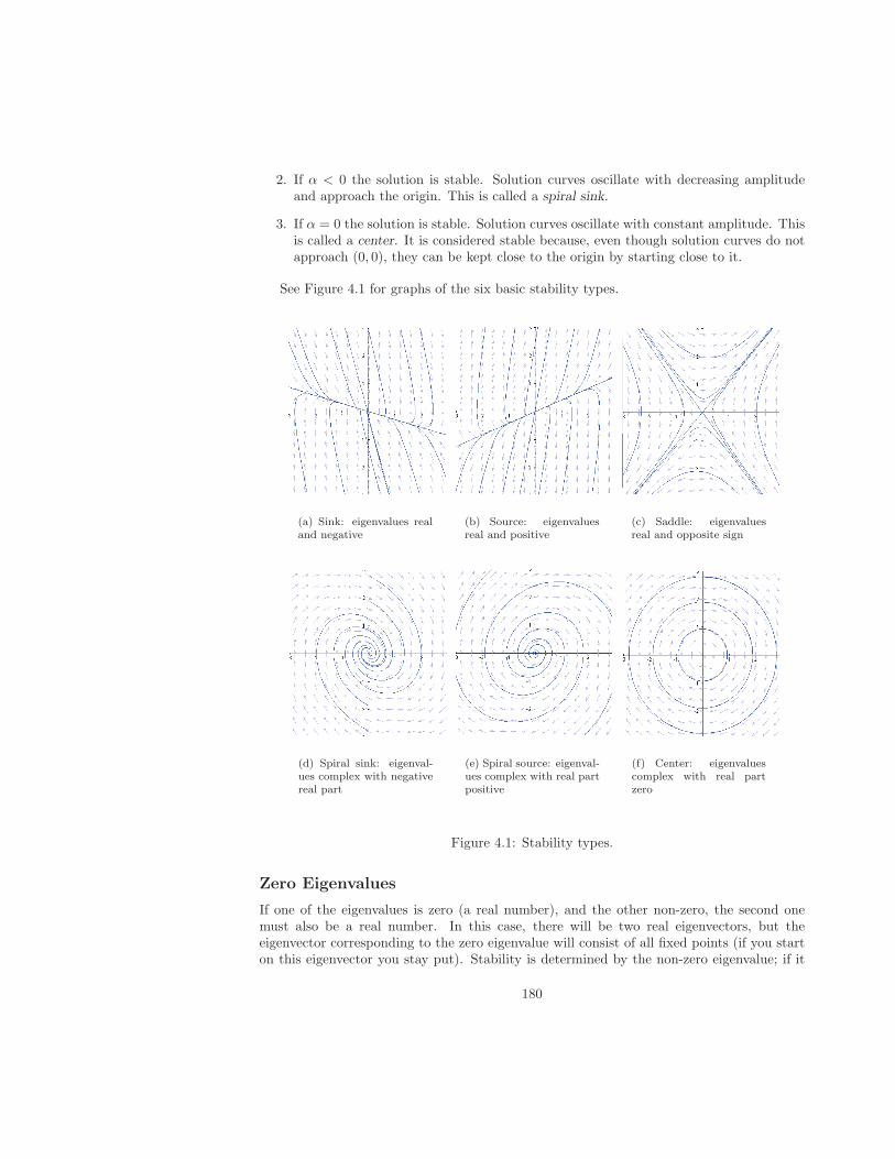
2. If α < 0 the solution is stable. Solution curves oscillate with decreasing amplitudeand approach the origin. This is called a spiral sink.
3. If α = 0 the solution is stable. Solution curves oscillate with constant amplitude. Thisis called a center. It is considered stable because, even though solution curves do notapproach (0, 0), they can be kept close to the origin by starting close to it.
See Figure 4.1 for graphs of the six basic stability types.
(a) Sink: eigenvalues realand negative
(b) Source: eigenvaluesreal and positive
(c) Saddle: eigenvaluesreal and opposite sign
(d) Spiral sink: eigenval-ues complex with negativereal part
(e) Spiral source: eigenval-ues complex with real partpositive
(f) Center: eigenvaluescomplex with real partzero
Figure 4.1: Stability types.
Zero Eigenvalues
If one of the eigenvalues is zero (a real number), and the other non-zero, the second onemust also be a real number. In this case, there will be two real eigenvectors, but theeigenvector corresponding to the zero eigenvalue will consist of all fixed points (if you starton this eigenvector you stay put). Stability is determined by the non-zero eigenvalue; if it
180
is positive the origin is unstable, and if it is negative the origin is stable (though solutioncurves do not necessarily approach the origin).
If both eigenvalues are zero, all the points in the plane are fixed points, are are stable,including the origin (not a very interesting case).
Example 4.2.1 For each system, determine the stability type of (0, 0).
1. x′ = x+ y, y′ = 4x+ y
2. x′ = x− y, y′ = 4x+ y
3. x′ = x, y′ = x+ 3y
4. x′ = y, y′ = −x
Solution.
1. A =
[1 14 1
]
. The eigenvalues are −1 and 3, so the origin is a saddle.
2. A =
[1 −14 1
]
. The eigenvalues are 1± 2i, so the origin is a spiral source..
3. A =
[1 01 3
]
. The eigenvalues are 1 and 3, so the origin is a source.
4. A =
[0 1−1 0
]
. The eigenvalues are ±i so the origin is a center.
The Trace-Determinant Plane
When the system is written in matrix form x′ = Ax, the trace and determinant of A can also
be used to determine the stability type of (0, 0). Recall that the determinant of A =
[a bc d
]
is ad− bc and the trace is a+ d.A theorem in linear algebra (not stated previously) states that the determinant of a
matrix is the product of the eigenvalues, and the trace is the sum of the eigenvalues. Thusr1 + r2 = trace(A) and r1r2 = det(A). If we solve these two equations for r1 and r2 we get
r1, r2 =1
2tr ± 1
2
√
tr2 − 4det =1
2tr ±
√
tr2
4− det
From this equation we can conclude (proof relegated to the exercises) that
1. If det < 0, the eigenvalues are real and opposite sign; this means (0, 0) is a saddle.
2. If 0 < det < tr2
4 the eigenvalues are real; if tr > 0 they are both positive (source) andif tr < 0 they are both negative (sink).
3. If det > tr2
4 the eigenvalues are complex; if tr > 0 the real part α > 0 (spiral source),if tr < 0 the real part α < 0 (spiral source), and if tr = 0 the real part α = 0 (center).
181
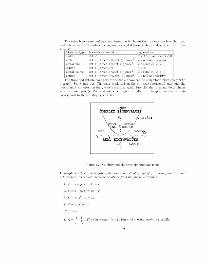
The table below summarizes the information in this section, by showing how the traceand determinant of A and/or the eigenvalues of A determine the stability type of (0, 0) forx′ = Ax
Stability type trace/determinant eigenvaluessaddle det < 0 one λ > 0 and one λ < 0sink det > 0,trace < 0, det ≤ 1
4 trace2 λ′s real and negative
spiral sink det > 0,trace < 0,det > 14 trace
2 λ′s complex, α < 0center det > 0,trace = 0 α = 0spiral source det > 0,trace > 0,det > 1
4 trace2 λ′s complex, α > 0
source det > 0,trace > 0, det ≤ 14 trace
2 λ′s real and positive
The trace and determinant part of the table above can be understood more easily witha graph. See Figure 4.2. The trace is plotted on the x − axis (horizontal axis) and thedeterminant is plotted on the y − axis (vertical axis). Just plot the trace and determinantas an ordered pair (tr, det) and see which region it falls in. The positive vertical axiscorresponds to the stability type center.
Figure 4.2: Stability and the trace determinant plane
Example 4.2.2 For each system, determine the stability type of (0, 0) using the trace anddeterminant. These are the same equations from the previous example.
1. x′ = x+ y, y′ = 4x+ y
2. x′ = x− y, y′ = 4x+ y
3. x′ = x, y′ = x+ 3y
4. x′ = y, y′ = −x
Solution.
1. A =
[1 14 1
]
. The determinant is −3. Since det < 0 the origin is a saddle.
182
2. A =
[1 −14 1
]
. The trace is 2 and the determimant is 5. Since 14 tr
2 = 1 we have
det > 14 tr
2 so the origin is a spiral source.
3. A =
[1 01 3
]
. The trace is 4 and the determinant is 3. Since 14 tr
2 = 4 we have
det < 14 tr
2 so the origin is a source.
4. A =
[0 1−1 0
]
. The trace is 0 and the determinant is 1. Thus the origin is a center.
Exercises 4.2 For each matrix A below, compute the trace and determinant. Use the trace-determinant plane to decide what type of equilibrium the system ~X′ = A~X has at (0, 0).
1. A =
(1 2−2 −2
)
2. A =
(2 3−1 0
)
3. A =
(−4 2−1 1
)
4. A =
(−1 11 −2
)
5. A =
(2 3−2 −2
)
6. A =
(1 21 3
)
For each system below, find the eigenpairs (you will probably want to use technologyfor this) and sketch by hand a phase portrait for the system. If the eigenvalues arereal, the eigenvectors should be included in the sketch. Put arrows on each solutiontrajectory to denote the direction of motion.
7. x′ = x+ 2y, y′ = −2x− 2y
8. x′ = 2x+ 3y, y′ = −x
9. x′ = −4x+ 2y, y′ = −x+ y
10. x′ = −x+ y, y′ = x− 2y
11. x′ = 2x+ 3y, y′ = −2x− 2y
12. x′ = x+ 2y, y′ = x+ 3y
For each mass-spring equation 13-18 below, write it as a system and use the trace-determinant plane or eigenvalues to determine the type of equilibrium at (0, 0). Howdoes the type of the equilibrium compare with the type of damping (undamped, underdamped, critically damped, or over damped)? Can you formulate a general statementabout this?
183
13. x′′ + 4x′ + 2x = 0
14. x′′ + 9x = 0
15. 3x′′ + 2x′ + x = 0
16. x′′ + x′ + 2x = 0
17. x′′ + 5x′ + 4x = 0
18. x′′ + 2x′ + x = 0
184
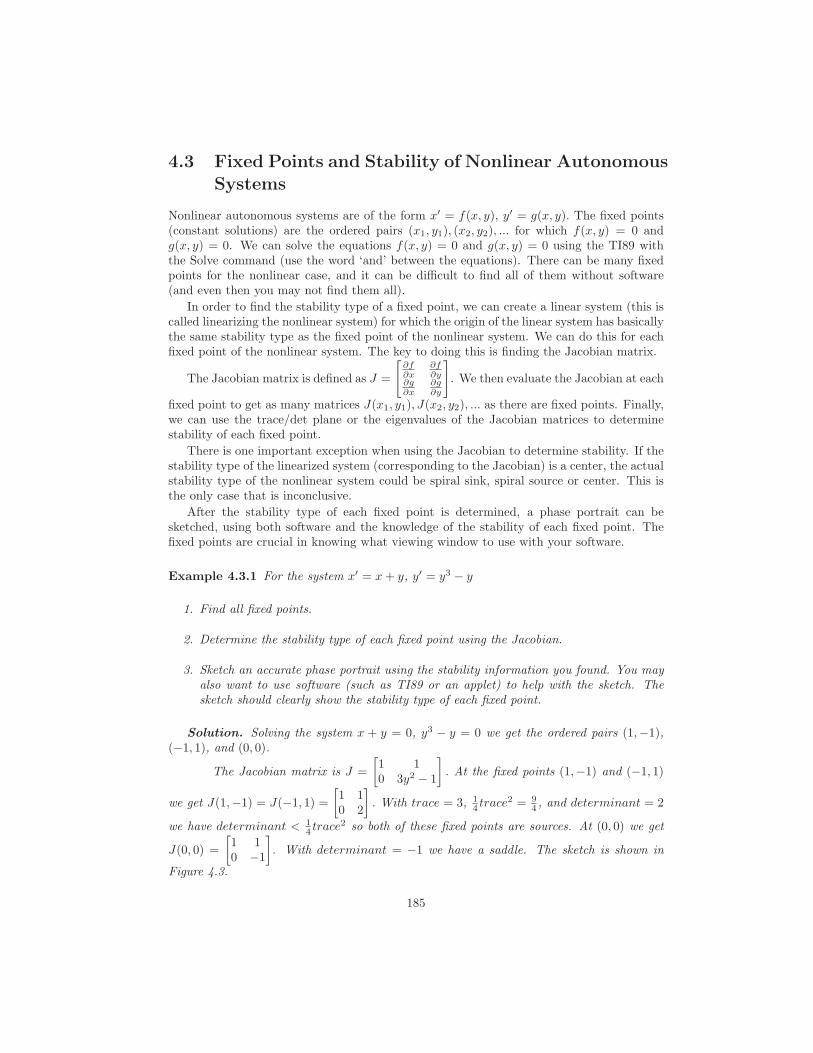
4.3 Fixed Points and Stability of Nonlinear Autonomous
Systems
Nonlinear autonomous systems are of the form x′ = f(x, y), y′ = g(x, y). The fixed points(constant solutions) are the ordered pairs (x1, y1), (x2, y2), ... for which f(x, y) = 0 andg(x, y) = 0. We can solve the equations f(x, y) = 0 and g(x, y) = 0 using the TI89 withthe Solve command (use the word ‘and’ between the equations). There can be many fixedpoints for the nonlinear case, and it can be difficult to find all of them without software(and even then you may not find them all).
In order to find the stability type of a fixed point, we can create a linear system (this iscalled linearizing the nonlinear system) for which the origin of the linear system has basicallythe same stability type as the fixed point of the nonlinear system. We can do this for eachfixed point of the nonlinear system. The key to doing this is finding the Jacobian matrix.
The Jacobian matrix is defined as J =
[∂f∂x
∂f∂y
∂g∂x
∂g∂y
]
. We then evaluate the Jacobian at each
fixed point to get as many matrices J(x1, y1), J(x2, y2), ... as there are fixed points. Finally,we can use the trace/det plane or the eigenvalues of the Jacobian matrices to determinestability of each fixed point.
There is one important exception when using the Jacobian to determine stability. If thestability type of the linearized system (corresponding to the Jacobian) is a center, the actualstability type of the nonlinear system could be spiral sink, spiral source or center. This isthe only case that is inconclusive.
After the stability type of each fixed point is determined, a phase portrait can besketched, using both software and the knowledge of the stability of each fixed point. Thefixed points are crucial in knowing what viewing window to use with your software.
Example 4.3.1 For the system x′ = x+ y, y′ = y3 − y
1. Find all fixed points.
2. Determine the stability type of each fixed point using the Jacobian.
3. Sketch an accurate phase portrait using the stability information you found. You mayalso want to use software (such as TI89 or an applet) to help with the sketch. Thesketch should clearly show the stability type of each fixed point.
Solution. Solving the system x + y = 0, y3 − y = 0 we get the ordered pairs (1,−1),(−1, 1), and (0, 0).
The Jacobian matrix is J =
[1 10 3y2 − 1
]
. At the fixed points (1,−1) and (−1, 1)
we get J(1,−1) = J(−1, 1) =
[1 10 2
]
. With trace = 3, 14 trace
2 = 94 , and determinant = 2
we have determinant < 14 trace
2 so both of these fixed points are sources. At (0, 0) we get
J(0, 0) =
[1 10 −1
]
. With determinant = −1 we have a saddle. The sketch is shown in
Figure 4.3.
185

Figure 4.3: Phase portrait for x′ = x+ y, y′ = y3 − y
Exercises 4.3 For each system below:a. Find all of the equilibrium points in the given region of the phase plane. If a region
is not given, choose an appropriate one based on the equilibrium points.b. Determine the stability type of each equilibrium point using the Jacobian. You may
use eigenvalues or trace/determinant.c. Use the information from parts a-c to sketch a phase portrait; you may also want to
use software to help.
1. x′ = y, y′ = −0.5y + x− x3
2. x′ = y, y′ = −0.5y − x+ x3
3. x′ = y, y′ = −0.5y + x− x2
4. x′ = y, y′ = −0.5y − x+ x2
5. Competing species model. The functions x(t) and y(t) represent the populationsize, at time t, of two competing species in the same ecosystem. Their growth equationsare given by
x′ = x(1− x)− xy
y′ = y(3
4− y)− 1
2xy.
Let x vary between 0 and 1.5, and y between 0 and 1.5.
6. Damped pendulum model. The second-order equation θ′′ + θ′ + 4 sin(θ) = 0 isconverted into the system
x′ = y
y′ = −4 sin(x)− y.
186
Let x vary between −8 and 8, and y between −10 and 10.
7. Predator-prey model. In this model, x(t) represents the number of predators attime t, and y(t) is the number of prey. Notice that the predators are affected positivelyby their interactions with the prey, while the affect of the interaction on the prey isnegative. If no prey are available, the predators will die out exponentially.
x′ = −x+ xy
y′ = 4y − 2xy.
Let x vary between 0 and 5, and y between 0 and 5.
187
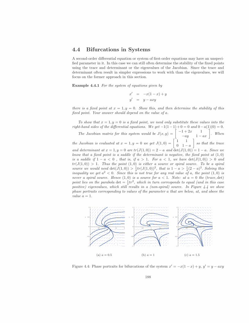
4.4 Bifurcations in Systems
A second-order differential equation or system of first-order equations may have an unspeci-fied parameter in it. In this case we can still often determine the stability of the fixed pointsusing the trace and determinant or the eigenvalues of the Jacobian. Since the trace anddeterminant often result in simpler expressions to work with than the eigenvalues, we willfocus on the former approach in this section.
Example 4.4.1 For the system of equations given by
x′ = −x(1− x) + y
y′ = y − axy
there is a fixed point at x = 1, y = 0. Show this, and then determine the stability of thisfixed point. Your answer should depend on the value of a.
To show that x = 1, y = 0 is a fixed point, we need only substitute these values into theright-hand sides of the differential equations. We get −1(1− 1)+0 = 0 and 0−a(1)(0) = 0.
The Jacobian matrix for this system would be J(x, y) =
[−1 + 2x 1−ay 1− ax
]
. When
the Jacobian is evaluated at x = 1, y = 0 we get J(1, 0) =
[1 10 1− a
]
so that the trace
and determinant at x = 1, y = 0 are tr(J(1, 0)) = 2− a and det(J(1, 0)) = 1− a. Since weknow that a fixed point is a saddle if the determinant is negative, the fixed point at (1, 0)is a saddle if 1 − a < 0 , that is, if a > 1. For a < 1, we have det(J(1, 0)) > 0 andtr(J(1, 0)) > 1. Thus the point (1, 0) is either a source or spiral source. To be a spiralsource we would need det(J(1, 0)) > 1
4 tr(J(1, 0))2, that is 1 − a > 1
4 (2 − a)2. Solving thisinequality we get a2 < 0. Since this is not true for any real value of a, the point (1, 0) isnever a spiral source. Hence (1, 0) is a source for a < 1. Note: at a = 0 the (trace, det)point lies on the parabola det = 1
4 tr2, which in turn corresponds to equal (and in this case
positive) eigenvalues, which still results in a (non-spiral) source. In Figure 4.4 we showphase portraits corresponding to values of the parameter a that are below, at, and above thevalue a = 1.
(a) a = 0.5 (b) a = 1 (c) a = 1.5
Figure 4.4: Phase portraits for bifurcations of the system x′ = −x(1− x) + y, y′ = y − axy
188
In many cases we want to determine the fixed points and their stability as the parametervaries. As with first-order differential equations, for systems of first-order equations we saythat a bifurcation occurs when the number of fixed points, or when the stability type ofone or more fixed points, changes as the parameter goes through some value (called thebifurcation value). Thus in Example 4.4.1 we have a bifurcation at a = 1.
In terms of the trace-determinant plane, we are looking for values of the parameter wherethe point (trace, det) crosses from one of the key regions of the trace-determinant plane intoanother (trace and det refer to the trace and determinant of the Jacobian at a given fixedpoint). We illustrate these ideas with two more examples.
Example 4.4.2 Consider the damped pendulum model from the exercises of the last section,given by
x′ = y
y′ = −4 sin(x)− ay.
where we have added the parameter a to represent the amount of damping in the system.For a > 0 there is positive damping, and for a < 0 there is negative damping. Negativedamping is not physically realistic in a real pendulum (it tends to speed up the pendulum inthe direction that it is already moving, rather than slowing it down), but we can still studythe mathematics for a either positive or negative.
Determine the bifurcation values in terms of the parameter a, that is, determine thevalues of a for which the number of fixed points or the stability type of any of the fixed pointschanges.
First we must determine the equilibrium points in terms of the parameter a. We gety = 0 and −4 sin(x) − ay = 0. This implies that sin(x) = 0, and so the equilibriumvalues are given by (0, 0), (±π, 0), (±2π, 0), ... or equivalently at (±nπ, 0) where n can be anynonnegative integer.
Next we find the Jacobian at each equilibrium point. We have J =
[0 1
−4 cos(x) −a
]
. At
the points (±nπ, 0) for n even we get Jn even(±nπ, 0) =
[0 1−4 −a
]
and for n odd we get
Jn odd(±nπ, 0) =
[0 14 −a
]
.
Now find the trace and determinant for each case. For both cases we get trace(J) = −a.For n even we get det(Jn even) = 4 and for n odd we get det(Jn odd) = −4. Thus, for n oddwe always have a saddle point. For n even, we can have a source, spiral source, spiral sinkor sink. Thus there will be 3 values of a at which bifurcations occur, all involving the fixedpoints at (±nπ, 0) for n even.
To find the bifurcation points, we only need to look at Jn even(±nπ, 0) =
[0 1−4 −a
]
. We
have trace
[0 1−4 −a
]
= −a and det
[0 1−4 −a
]
= 4. Letting a vary from −∞ to ∞, the
first bifurcation occurs when the point (trace, det) = (−a, 4) crosses from the source regionto the spiral source region . This would be when 4 = 1
4a2 (with a < 0), and hence when
a = −4. The next bifurcation occurs when the point (trace, det) = (−a, 4) crosses from thespiral source region to the spiral sink region, which is when trace = −a = 0, and hence
189
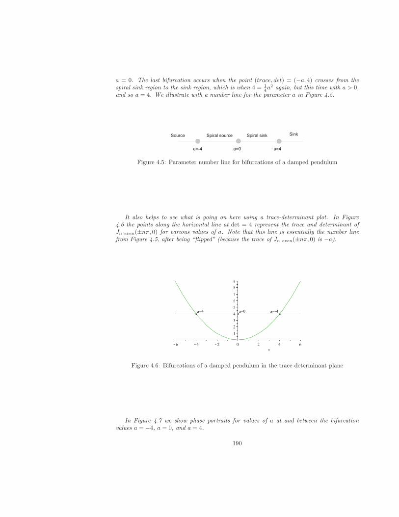
a = 0. The last bifurcation occurs when the point (trace, det) = (−a, 4) crosses from thespiral sink region to the sink region, which is when 4 = 1
4a2 again, but this time with a > 0,
and so a = 4. We illustrate with a number line for the parameter a in Figure 4.5.
Figure 4.5: Parameter number line for bifurcations of a damped pendulum
It also helps to see what is going on here using a trace-determinant plot. In Figure4.6 the points along the horizontal line at det = 4 represent the trace and determinant ofJn even(±nπ, 0) for various values of a. Note that this line is essentially the number linefrom Figure 4.5, after being “flipped” (because the trace of Jn even(±nπ, 0) is −a).
a=-4a=0a=4
x
K6 K4 K2 0 2 4 6
1
2
3
4
5
6
7
8
9
Figure 4.6: Bifurcations of a damped pendulum in the trace-determinant plane
In Figure 4.7 we show phase portraits for values of a at and between the bifurcationvalues a = −4, a = 0, and a = 4.
190
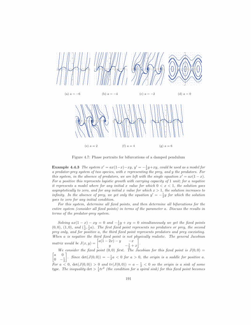
(a) a = −6 (b) a = −4 (c) a = −2 (d) a = 0
(e) a = 2 (f) a = 4 (g) a = 6
Figure 4.7: Phase portraits for bifurcations of a damped pendulum
Example 4.4.3 The system x′ = ax(1−x)−xy, y′ = − 12y+xy, could be used as a model for
a predator-prey system of two species, with x representing the prey, and y the predators. Forthis system, in the absence of predators, we are left with the single equation x′ = ax(1− x).For a positive this represents logistic growth with carrying capacity of 1 unit; for a negativeit represents a model where for any initial x value for which 0 < x < 1, the solution goesasymptotically to zero, and for any initial x value for which x > 1, the solution increases toinfinity. In the absence of prey, we get only the equation y′ = − 1
2y for which the solutiongoes to zero for any initial condition.
For this system, determine all fixed points, and then determine all bifurcations for theentire system (consider all fixed points) in terms of the parameter a. Discuss the results interms of the predator-prey system.
Solving ax(1 − x) − xy = 0 and − 12y + xy = 0 simultaneously we get the fixed points
(0, 0), (1, 0), and ( 12 ,12a). The first fixed point represents no predators or prey, the second
prey only, and for positive a, the third fixed point represents predators and prey coexisting.When a is negative the third fixed point is not physically realistic. The general Jacobian
matrix would be J(x, y) =
[a(1− 2x)− y −x
y − 12 + x
]
.
We consider the fixed point (0, 0) first. The Jacobian for this fixed point is J(0, 0) =[a 00 − 1
2
]
. Since det(J(0, 0)) = − 12a < 0 for a > 0, the origin is a saddle for positive a.
For a < 0, det(J(0, 0)) > 0 and tr(J(0, 0)) = a − 12 < 0 so the origin is a sink of some
type. The inequality det > 14 tr
2 (the condition for a spiral sink) for this fixed point becomes
191
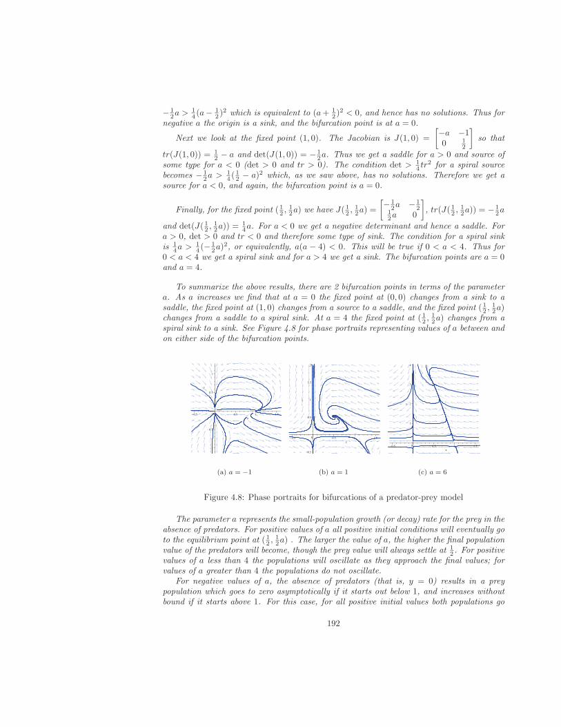
− 12a > 1
4 (a− 12 )
2 which is equivalent to (a+ 12 )
2 < 0, and hence has no solutions. Thus fornegative a the origin is a sink, and the bifurcation point is at a = 0.
Next we look at the fixed point (1, 0). The Jacobian is J(1, 0) =
[−a −10 1
2
]
so that
tr(J(1, 0)) = 12 − a and det(J(1, 0)) = − 1
2a. Thus we get a saddle for a > 0 and source ofsome type for a < 0 (det > 0 and tr > 0). The condition det > 1
4 tr2 for a spiral source
becomes − 12a > 1
4 (12 − a)2 which, as we saw above, has no solutions. Therefore we get a
source for a < 0, and again, the bifurcation point is a = 0.
Finally, for the fixed point ( 12 ,12a) we have J( 12 ,
12a) =
[− 1
2a − 12
12a 0
]
, tr(J( 12 ,12a)) = − 1
2a
and det(J( 12 ,12a)) =
14a. For a < 0 we get a negative determinant and hence a saddle. For
a > 0, det > 0 and tr < 0 and therefore some type of sink. The condition for a spiral sinkis 1
4a > 14 (− 1
2a)2, or equivalently, a(a − 4) < 0. This will be true if 0 < a < 4. Thus for
0 < a < 4 we get a spiral sink and for a > 4 we get a sink. The bifurcation points are a = 0and a = 4.
To summarize the above results, there are 2 bifurcation points in terms of the parametera. As a increases we find that at a = 0 the fixed point at (0, 0) changes from a sink to asaddle, the fixed point at (1, 0) changes from a source to a saddle, and the fixed point ( 12 ,
12a)
changes from a saddle to a spiral sink. At a = 4 the fixed point at ( 12 ,12a) changes from a
spiral sink to a sink. See Figure 4.8 for phase portraits representing values of a between andon either side of the bifurcation points.
(a) a = −1 (b) a = 1 (c) a = 6
Figure 4.8: Phase portraits for bifurcations of a predator-prey model
The parameter a represents the small-population growth (or decay) rate for the prey in theabsence of predators. For positive values of a all positive initial conditions will eventually goto the equilibrium point at ( 12 ,
12a) . The larger the value of a, the higher the final population
value of the predators will become, though the prey value will always settle at 12 . For positive
values of a less than 4 the populations will oscillate as they approach the final values; forvalues of a greater than 4 the populations do not oscillate.
For negative values of a, the absence of predators (that is, y = 0) results in a preypopulation which goes to zero asymptotically if it starts out below 1, and increases withoutbound if it starts above 1. For this case, for all positive initial values both populations go
192

extinct (asymptotically). Note that when there are few predators initially, and the initialprey population is above 1, the prey increase dramatically at first, but eventually enoughpredators enter to drive the system back to extinction.
Exercises 4.4 For each system below, find all equilibrium points, and bifurcation values forthe given parameter
1. x′ = y, y′ = −ax− y
2. x′ = y, y′ = −x− by
The differential equation x′′ + ax′ + x3 − bx = 0 can be used to model a “double wellpotential” mechanical system (in the literature it is referred to as a Duffing equation).An example of such a system would be an upright flexible beam, fixed at the bottom butfree at the top, with x measuring the distance from the vertical at the top of the beam.If the beam is flexible enough, it will flop to the left or right and come to rest there. Theparameter a represents the amount of damping in the system, and b is a measure howfar the beam will flop to either side when it comes to rest (a measure of the rigidity ofthe beam). When put into system form this equation becomes x′ = y, y′ = −ay−x3+bx(show this). For the next two problems below, find all equilibrium points for eachsystem in terms of the given parameter, and then find the trace and determinant ofthe Jacobian matrix for each fixed point. Using this information find all bifurcationvalues in terms of the given parameter for each system. Explain what this means interms of the mechanical system. Consider all values of each parameter, even physicallyunrealistic ones.
3. x′ = y, y′ = −ay − x3 + x
4. x′ = y, y′ = −y − x3 + bx
The system x′ = x(1−x)−axy, y′ = −y+ bxy can be used as a model for a predator-prey system, with x representing the number of prey, and y representing the numberof predators (see the third example from this section). The parameter a representsthe degree to which interactions between the species subtracts from the prey, and brepresents the degree to which interactions between the species adds to the predators.For the next two problems below, find all equilibrium points for each system in terms ofthe given parameter, and then find the trace and determinant of the Jacobian matrixfor each fixed point. Using this information find all bifurcation values in terms of thegiven parameter for each system. Explain what this means in terms of the predator-prey system. Consider all values of each parameter, even physically unrealistic ones.
5. x′ = x(1− x)− axy, y′ = −y + xy
6. x′ = x(1− x)− xy, y′ = −y + bxy
193

194
Chapter 5
Laplace Transforms
In this chapter we introduce yet another method for solving linear differential equations.The method applies to linear equations of any order. Although we already have methods forsolving linear equations with constant coefficients, the method of Laplace Transforms givesthe solution in a slightly different form; instead of arbitrary constants, the solution containsthe initial conditions directly. This method is also very useful for non-homogeneous problemswhere the forcing function is defined piecewise, or contains an impulse function (impulsefunctions have not been encountered yet). Finally, this method is useful for interpretingsolutions to mass-spring problems and to electrical circuit problems.
5.1 Simple Laplace Transforms
In this section we introduce the concept of the Laplace transform, and find a few useful,but elementary, transforms. We then demonstrate how to solve differential equations usingLaplace transforms, in cases where the differential equation is relatively simple.
Definition 5.1 The Laplace transform of a function f(t), t > 0, is a new function F (s)defined as
F (s) =
∫ ∞
0
e−stf(t)dt.
We also use the notationF (s) = L[f(t)]
where L is called the Laplace operator.
The Laplace transform turns a function of t into a different function of s; or, as anengineer might say, it transforms a function from the t-domain into the s-domain. We willuse the convention that lower case letters such as f , g, and h, represent functions of t,and the corresponding upper case letters F , G, and H, represent the Laplace transforms ofthose functions (and hence are functions of s). Our goal is first to build a table of Laplacetransforms for the functions that come up frequently in differential equations; exponentialfunctions, trig functions, and polynomials. We will also need a few general properties ofLaplace transforms, that apply to arbitrary functions. It will then be shown how to solvecertain differential equations using these new tools.
195
Note that the integral, in the definition of the Laplace transform, is an improper integral ;and in Calculus you were taught to evaluate it as a limit:
∫ ∞
0
e−stf(t)dt ≡ limB→∞
∫ B
0
e−stf(t)dt.
When working with Laplace transforms, we will require that any function f(t) that is to betransformed must be at least piecewise continuous and of exponential order.
Definition 5.2 A function f(t) is said to be of exponential order if there exist positiveconstants M,a and T such that
|f(t)| < Meat for all t ≥ T.
With this assumption, the integral∫∞0
e−stf(t)dt and expressions such as e−stf(t)|t=∞t=0
will always be defined for s large enough; that is, we will not have to worry about theexistence of limits as t → ∞.
Theorem 5.1 The Laplace transforms of the functions eat, cos(bt), sin(bt), and tn, as wellas the constant function c, are given in the table below. In the table a, b and c can be anyreal numbers, and n ≥ 0 is an integer.
formulafunctionf(t)
Laplace transformF (s) = L[f(t)]
1 c cs , s > 0
2 eat 1s−a , s > a
3 cos(bt) ss2+b2 , s > 0
4 sin(bt) bs2+b2 , s > 0
5 tn n!sn+1 , s > 0
Proof: The first two formulas are quite easy to establish, and we will prove them here.The proofs of the next three will be done in the exercises. For 1 we have
F (s) = L[c] =
∫ ∞
0
e−stcdt = − c
se−st
∣∣∣
t=∞
t=0= 0 +
c
s
provided that s > 0. Similarly for 2
F (s) = L[eat] =
∫ ∞
0
e−steatdt =
∫ ∞
0
e(−s+a)tdt =1
−s+ ae(−s+a)t
∣∣∣∣
t=∞
t=0
=1
−s+ ae−∞ − 1
−s+ ae0 =
1
s− a
as long as s > a (and hence −s+ a is negative).
In order to effectively use Laplace transforms we also need a few rules that apply tofunctions in general, rather than to specific functions.
196
Theorem 5.2 The Laplace transforms in the table below apply to arbitrary functions f(t)and g(t), whose Laplace transforms are F (s) and G(s) respectively, and real number con-stants a and b.
formula function Laplace transform
6 f(t) F (s)7 af(t) + bg(t) aF (s) + bG(s)8 f ′(t) sF (s)− f(0)9 f ′′(t) s2F (s)− sf(0)− f ′(0)
Proof: Six in the table is just the definition of the Laplace transform, included here forcompleteness. Seven follows easily from the definition of the Laplace transform and theproperties of integration:
L[af(t) + bg(t)] =
∫ ∞
0
e−st(af(t) + bg(t))dt = a
∫ ∞
0
e−stf(t)dt+ b
∫ ∞
0
e−stg(t)dt
= aL[f(t)] + bL[g(t)] = aF (s) + bG(s).
Eight in the table is derived using integration by parts:
L[f ′(t)] =
∫ ∞
0
e−stf ′(t)dt = e−stf(t)∣∣t=∞
t=0−∫ ∞
0
−se−stf(t)dt
= 0− f(0) + s
∫ ∞
0
e−stf(t)dt = −f(0) + sF (s).
provided that limt→∞ e−stf(t) = 0 for s > a, for some a (and this can be seen to be true forany f(t) of exponential order). Nine can be proven using eight; we leave the details to theexercises.
Comment: Seven is a very important property, called linearity (it implies that theLaplace operator is a linear operator). Another way to state property seven using theLaplace operator is
L[af(t) + bg(t)] = aL[f(t)] + bL[g(t)].
The basic idea with linear operators is that you can “distribute” them, and then pull outconstants.
Example 5.1.1 Find the Laplace transform of 2e−3t + 4 sin(5t)− 6t7.
Using linearity we have
L[2e−3t + 4 sin(5t)− 6t7] = 2L[e−3t] + 4L[sin(5t)]− 6L[t7].
Next we apply formulas 2 (a = −3), 4 (b = 5), and 5 (n = 7):
2L[e−3t] + 4L[sin(5t)]− 6L[t7] = 21
s+ 3+ 4
5
s2 + 25− 6
7!
s8
=2
s+ 3+
20
s2 + 25− 30240
s8
197
Example 5.1.2 Find the Laplace transform of both sides of the differential equation y′ −2y = 3 cos(4t). Then equate the transforms of both sides and solve for Y (s), the transformof the solution y(t).
On the left-hand side we use linearity followed by formulas 6 and 8:
L[y′ − 2y] = L[y′]− 2L[y] = sY (s)− y(0)− 2Y (s).
On the right-hand side, we use linearity followed by formula 3 (b = 4):
L[3 cos(4t)] = 3L[cos(4t)] = 3s
s2 + 16.
Equating the transforms of both sides we get
sY (s)− y(0)− 2Y (s) =3s
s2 + 16.
Then we move terms that do not have Y (s) in them to the right side, and factor out Y (s)on the left:
Y (s)(s− 2) =3s
s2 + 16+ y(0).
Finally, we divide by (s− 2) and distribute to get
Y (s) =3s
s2+16 + y(0)
s− 2=
3s
(s2 + 16)(s− 2)+
y(0)
s− 2.
Solving differential equations and the Inverse Laplace transformIn example 5.1.2 we came close to solving the given differential equation; all we need
to do is recover the solution y(t) from its transform Y (s). In order to go from the Laplacetransform of a function back to the original function we must apply the inverse Laplacetransform. We use the symbol L−1 to denote the inverse Laplace transform operator. Thus,if F (s) = L[f(t)], then f(t) = L−1[F (s)]. Just as the Laplace transform takes us fromthe left column to the right column for formulas 1-9 in Theorems 5.1 and 5.2, the inverseLaplace transform takes us from the right column to the left column.
Theorem 5.3 The inverse Laplace transform is a linear operator; that is, L−1[aF (s) +bG(s)] = aL−1[F (s)] + bL−1[G(s)].
Proof. Apply L−1 to both sides of L[af(t) + bg(t)] = aL[f(t)] + bL[g(t)].
In order to apply the inverse Laplace transform effectively in solving differential equa-tions, we need one more tool. Looking back at example 5.1.2, in order to finish off the
problem and find the inverse Laplace transform of Y (s) we need to find L−1[
3s(s2+16)(s−2)
]
.
Since there is no form in the right column of formulas 1-9 in Theorems 5.1 and 5.2 that cor-responds to this function of s, we need to apply a procedure that you may have encounteredin a calculus course: partial fractions.
198
Review of partial fractions
The idea of partial fractions is to rewrite a rational function (a ratio of two polynomials),whose denominator is of higher degree than the numerator, by factoring the denominator,and expressing that rational function as a sum of new rational functions, whose denominatorsare the factors of the denominator of the original function. For example, 1
(x−1)(x−2) can be
rewritten as 1x−2 − 1
x−1 (show this). In example 5.1.2, 3s(s2+16)(s−2) can be rewritten as
3/10s−2 +
( 125− 3
10s)
s2+16 = 310
1s−2 + 12
51
s2+16 − 310
ss2+16 after which the inverse Laplace transform
can easily be found (see the next example).
Partial fractions procedure:
Step 1: Starting with a rational function P (s)/Q(s), with the degree of the polyno-mial Q(s) greater than that of P (s), factor the denominator into linear and non-factorablequadratic factors (we consider only real-valued factors). The single linear factors will havethe form as+b and the quadratic factors will have the form as2+bs+c, with b2−4ac < 0 (ifb2 − 4ac ≥ 0 then the quadratic factor can itself be factored into linear factors). Repeatedlinear factors will be of the form (as+ b)n for some integer n ≥ 2.
Step 2: For the partial fraction expansion, assume the form Aas+b for each single linear
factor in the denominator, assume the form Bs+Cas2+bs+c for each single quadratic factor, and
assume the form Das+b +
E(as+b)2 + . . .+ Z
(as+b)n for each repeated linear factor (as+ b)n. We
do not consider repeated quadratic factors, or any higher order factors, although these canbe easily handled by computer algebra systems.
Step 3: Set the rational function from Step 1 equal to the sum of the assumed forms fromStep 2, find a common denominator, and then equate and multiply out the numerators.
Step 4: Equate coefficients of like terms from the equation in Step 3. This will giveyou n linear equations in n unknowns A, B, C, ... . Solve the set of equations in Step 3using a standard technique such as Gaussian elimination, or even better, using a graphingcalculator or computer program.
Example 5.1.3 Find the partial fraction expansion for s+2(s+1)(s−1)2(s2+1) .
Step 1 is done since the denominator is already factored as much as possible, so we goto Steps 2 and 3 and assume
s+ 2
(s+ 1)(s− 1)2(s2 + 1)=
A
s+ 1+
Bs+ C
s2 + 1+
D
s− 1+
E
(s− 1)2.
The common denominator is (s+ 1)(s− 1)2(s2 + 1) so
s+ 2
(s+ 1)(s− 1)2(s2 + 1)=
A(s− 1)2(s2 + 1)
(s+ 1)(s− 1)2(s2 + 1)+
(Bs+ C)(s+ 1)(s− 1)2
(s+ 1)(s− 1)2(s2 + 1)
+D(s+ 1)(s− 1)(s2 + 1)
(s+ 1)(s− 1)2(s2 + 1)+
E(s+ 1)(s2 + 1)
(s+ 1)(s− 1)2(s2 + 1)
199
or after equating and multiplying out the numerators
s+ 2 = A− 2As+ 2As2 − 2As3 +As4
+C +Bs− Cs−Bs2 − Cs2 −Bs3 + Cs3 +Bs4
−D + s4D
+E + sE + s2E + s3E
Finally we go to Step 4 and equate the coefficients of the various powers of s on both sides ofthe equation (as well as the constant terms without s, as they can be considered coefficientsof s0 = 1). This results in the following 5 linear equations in 5 unknowns:
s4 : 0 = A+B +D
s3 : 0 = −2A−B + C + E
s2 : 0 = 2A−B − C + E
s : 1 = −2A+B − C + E
constants (s0) : 2 = A+ C −D + E
Solving this system using the solve command of a graphing calculator or computer softwarewe get
A =1
8, B =
3
4, C =
1
4, D = −7
8, E =
3
4
thus we can write
s+ 2
(s+ 1)(s− 1)2(s2 + 1)=
18
s+ 1+
34s+
14
s2 + 1−
78
s− 1+
34
(s− 1)2.
The good news is that if we have a computer algebra system available, we can get partialfraction expansions directly. Most computer algebra systems have a command (such asexpand, on the TI-89 or TI-92) which will take a rational function as argument and produceits partial fraction expansion. From this point forward in the text, we will not explicitlyderive partial fraction expansions, but will assume that the student is either comfortabledoing them by hand as in the previous example, or has a computer algebra system available(preferably both).
Three step procedure for solving linear differential equations using Laplacetransforms:
Step 1 Take the Laplace transform of both sides of the differential equation.Step 2 Solve for the transform of the solution Y (s).Step 3 Find the inverse Laplace transform of Y (s) to get the solution y(t).
Example 5.1.4 Use Laplace transforms to find the solution to the differential equationy′ − 2y = 3 cos(4t). This is the same differential equation as in Example 5.1.2.
200

In Example 5.1.2 we took the Laplace transform of both sides of the differential equation,and solved for Y (s) (Steps 1 and 2 above) to get
Y (s) =3s
s2+16 + y(0)
s− 2=
3s
(s2 + 16)(s− 2)+
y(0)
s− 2.
In order to find L−1[Y (s)] we need to do a partial fractions expansion. We know that theform of the expansion will be
3s
(s2 + 16)(s− 2)=
A
s− 2+
Bs+ C
s2 + 16.
We can find the values of A, B, and C as in Example 5.1.3 (find a common denominator,equate numerators, multiply out, equate coefficients of like terms, solve the resulting linearsystem), or we can use technology (e.g. the expand command of the TI-89). In either casewe get
3s
(s2 + 16)(s− 2)=
310
(s− 2)+
− 310s+
125
s2 + 16.
We next multiply out the second term, apply L−1, and use linearity to get
L−1
[3s
(s2 + 16)(s− 2)
]
=3
10L−1
[1
(s− 2)
]
− 3
10L−1
[s
s2 + 16
]
+12
5L−1
[1
s2 + 16
]
The goal is now to get each expression in brackets above into a form where each term appearsin the right column of the table of Laplace transforms in Theorem 5.1 (formulas 1-5). Thefirst two terms correspond to formulas 2 and 3 respectively. The third term needs a minoradjustment to fit formula 4; we need
√16 = 4 in the numerator, so using linearity we write
L−1[
1s2+16
]
= 14L
−1[
4s2+16
]
to get
L−1
[3s
(s2 + 16)(s− 2)
]
=3
10L−1
[1
(s− 2)
]
− 3
10L−1
[s
s2 + 16
]
+12
5· 14L−1
[4
s2 + 16
]
=3
10e2t − 3
10cos(4t) +
3
5sin(4t).
Finally, we get
y(t) = L−1[Y (s)] = L−1
[3s
(s2 + 16)(s− 2)+
y(0)
s− 2
]
= L−1
[3s
(s2 + 16)(s− 2)
]
+ L−1
[y(0)
s− 2
]
= L−1
[3s
(s2 + 16)(s− 2)
]
+ y(0)L−1
[1
s− 2
]
=3
10e2t − 3
10cos(4t) +
3
5sin(4t) + y(0)e2t.
201
Example 5.1.5 Solve the initial value problem y′′ + y = sin(2t), y(0) = 3, y′(0) = 0 usingLaplace transforms.
Here we put it all together, and see the solution to a differential equation from beginningto end. Taking the Laplace transform of both sides and using linearity (formula 7, Theorem5.2) we have
L[y′′] + L[y] = L[sin(2t)].
On the left side we use formulas 6 and 9 from Theorem 5.2, and on the right we use formula4 from 5.1 to get
s2Y (s)− sy(0)− y′(0) + Y (s) =2
s2 + 4.
Putting in the initial conditions, and solving for Y (s) we get
s2Y (s)− 3s+ Y (s) =2
s2 + 4
Y (s)(s2 + 1) =2
s2 + 4+ 3s
Y (s) =2
s2+4 + 3s
s2 + 1=
2
(s2 + 4)(s2 + 1)+
3s
s2 + 1
Using partial fractions on the first term, we assume 2(s2+4)(s2+1) =
As+Bs2+4 + Cs+D
s2+1 and then
solve for the constants, or use the expand command of a computer algebra system to get
2
(s2 + 4)(s2 + 1)= −
23
s2 + 4+
23
s2 + 1.
We now use the inverse Laplace transform to get
y(t) = L−1[Y (s)] = L−1
[
−23
s2 + 4+
23
s2 + 1+
3s
s2 + 1
]
= L−1
[
−23
s2 + 4
]
+ L−1
[ 23
s2 + 1
]
+ L−1
[3s
s2 + 1
]
= −1
3L−1
[2
s2 + 4
]
+2
3L−1
[1
s2 + 1
]
+ 3L−1
[s
s2 + 1
]
= −1
3sin(2t) +
2
3sin(t) + 3 cos(t).
You should determine which formulas were used at each step.
Exercises 5.1 Find the Laplace transforms for the functions in 1-4 below, using formulas1-5 from Theorem 5.1 and linearity.
1. cos(t) + 2et.
2. 3− 2t+ 4t2.
3. − sin(3t)− 2t5 + 5
202

4. 3e−7t + 4 cos(8t)− 3 + 5t2
For exercises 5-8, find the Laplace transform of both sides of the differential equation,and then solve for Y (s).
5. y′ = y + 2
6. y′ + 2y = 4 sin(3t)
7. y′′ + 4y = cos(t)
8. y′′ + 4y = cos(2t)
For exercises 9-12, find the inverse Laplace transform of Y (s) to get y(t).
9. Y (s) = 2s−5 − 3s
s2+4 + 1s2
10. Y (s) = 2s+5 − 3
s2+9 − 10s5
11. Y (s) = 22s+5 − 3s
s2+2 + 15s2
12. Y (s) = 23s−5 − 3
2s2+4 + 13s
For exercises 13-16 solve the differential equation or initial value problem using thethree step procedure given in the text.
13. y′′ + 4y = cos(t), y(0) = 2, y′(0) = 0
14. y′ + 2y = 4 sin(3t), y(0) = 3
15. y′′ + 4y = 0
16. y′ = y + 2
Use integration to prove the following formulas.
17. L[cos(bt)] = sb2+s2 . (formula 3)
Note: If you are familiar with complex numbers, it is easier to find L[eibt] and take itsreal part.
18. L[sin(bt)] = bb2+s2 . (formula 4)
See note in the previous example.
19. L[tn] = n!xn+1 , for any integer n ≥ 0. (formula 5)
Hint: first show that L[t0] ≡ L[1] = 1/s and then use integration by parts to show thatL[tn] = n
sL[tn−1].
20. Apply formula 8 to the function f ′(t), to prove the formula L[f ′′(t)] = s2F (s)−sf(0)−f ′(0).
203
5.2 Deriving More Laplace Transforms
In order to solve more differential equations of interest (in the last section all of our secondorder equations were missing the y′ term), we need a few more Laplace transform rules, andan algebraic technique that you likely first (and probably last) saw in high school.
We start with two rules that are of the general type; that is, they apply to generalfunctions f(t) as do the rules from Theorem 5.2 in the previous section. We will then showhow to derive new specific Laplace transform rules using these general rules.
Theorem 5.4 The Laplace transforms in the table below apply to a general function f(t),whose Laplace transform is F (s), and to the arbitrary constant a.
formula function Laplace transform
10 eatf(t) F (s− a)
11 tnf(t) (−1)nF (n)(s)
Note: F (n)(s) represents the nth derivative of F (s)with respect to s .
Proof: The proofs of formulas 10 and 11 are left to the exercises.
Example 5.2.1 Derive rules for the Laplace transforms of eat cos(bt) and eat sin(bt).
We want to apply formula 10 with f(t) = cos(bt), but we first need to find F (s). We get
F (s) = L[f(t)] = L[cos(bt)] =s
s2 + b2
from formula 3 of Theorem 5.1. Now applying formula 10 we get
L[eat cos(bt)] = F (s− a) =s− a
(s− a)2 + b2.
Similarly
L[eat sin(bt)] =b
(s− a)2 + b2
where this time F (s) = bs2+b2 from formula 4 of Theorem 5.1.
Example 5.2.2 Derive rules for the Laplace transforms of t cos(bt) and t sin(bt).
To find L[t cos(bt)] we want to apply formula 11 with f(t) = cos(bt); we have F (s) =L[f(t)] = L[cos(bt)] = s
s2+b2 as in the previous example. Now applying formula 11 withn = 1 we get
L[t cos(bt)] = (−1)F ′(s) = (−1)(1)(s2 + b2)− (s)(2s)
(s2 + b2)2
(quotient rule)
=s2 − b2
(s2 + b2)2 .
204

Similarly to find L[t sin(bt)] we use F (s) = bs2+b2 and hence
L[t sin(bt)] = (−1)F ′(s) = − (0)(s2 + b2)− (b)(2s)
(s2 + b2)2
=2bs
(s2 + b2)2 .
Example 5.2.3 Derive a rule for the Laplace transform of tneat.
To find L[tneat] we choose to apply formula 10 from above with f(t) = tn. We haveF (s) = L[f(t)] = L[tn] = n!
sn+1 from Theorem 5.1, formula 5, and so applying formula 10we get
L[tneat] = F (s− a) =n!
(s− a)n+1.
Note: We could alternatively have used formula 11 from above; we leave this approachto the exercises.
We summarize the results of the last three examples in Table form:
formula function Laplace transform
12 eat cos(bt) s−a(s−a)2+b2
13 eat sin(bt) b(s−a)2+b2
14 t cos(bt) s2−b2
(s2+b2)2
15 t sin(bt) 2bs(s2+b2)2
16 tneat n!(s−a)n+1
Table 1: Derived Laplace transforms
Example 5.2.4 Solve the initial value problem y′′ + 2y′ + y = 0, y(0) = 3, y′(0) = 0using Laplace transforms.
We use the three step process: take the Laplace transform of both sides, solve for Y (s),then find the inverse Laplace transform of Y (s) to get y(t). Applying the Laplace operatorL to both sides of the differential equation, using linearity, and substituting 3 for y(0) and0 for y′(0) we get
L[y′′ + 2y′ + y] = L[y′′] + 2L[y′] + L[y]
= s2Y (s)− sy(0)− y′(0) + 2 (sY (s)− y(0)) + Y (s)
= s2Y (s)− 3s+ 2sY (s)− 6 + Y (s) = L[0] = 0.
Then solving the last line above for Y (s) we get
s2Y (s) + 2sY (s) + Y (s) = 3s+ 6
thus Y (s)(s2 + 2s+ 1
)= 3s+ 6
and so Y (s) =3s+ 6
s2 + 2s+ 1
205
We now factor the denominator s2 + 2s + 1 = (s + 1)2 and expand the fraction into twoterms to get
Y (s) =3s+ 6
(s+ 1)2=
3s
(s+ 1)2+
6
(s+ 1)2.
Neither of the two terms of Y (s) corresponds to the right column of our Laplace transformtables exactly as is, so we must make some adjustments. For the first term 3s
(s+1)2 we observe
that if instead of s in the numerator we had (s+ 1), then we could cancel and get a matchwith formula 2 from the previous section. Thus we both add and subtract the number 1 asfollows:
3s
(s+ 1)2=
3(s+ 1− 1)
(s+ 1)2=
3(s+ 1)− 3
(s+ 1)2
=3(s+ 1)
(s+ 1)2− 3
(s+ 1)2
=3
(s+ 1)− 3
(s+ 1)2
We now can combine some terms to get
Y (s) =3s
(s+ 1)2+
6
(s+ 1)2
=3
(s+ 1)− 3
(s+ 1)2+
6
(s+ 1)2
= .3
(s+ 1)+
3
(s+ 1)2
Finally we use linearity to get
y(t) = L−1 [Y (s)] = L−1
[3
(s+ 1)+
3
(s+ 1)2
]
= 3L−1
[1
(s+ 1)
]
+ 3L−1
[1
(s+ 1)2
]
= 3e−t + 3te−t
using formula 2 with a = −1 on the first term and formula 16 with n = 1 and a = −1 onthe second.
Before going much further, we need to review a technique that you probably first en-countered in high school, called “completing the square”.
Review of Completing the SquareThe idea of completing the square is to write a quadratic factor as the sum of a squared
linear factor and a constant (both possibly multiplied by another constant). We illustratehow to complete the square using 2s2 + 16s+ 64 as an example:
1. Factor out the lead coefficient a = 2 to get 2(s2 + 8s+ 32).
206

2. Take half of the coefficient of s in step 1 ( 12 (8) = 4 in this case) and then square thatnumber (42 = 16).
3. Add and subtract the result from step 2 inside the expression in step 1 to get 2(s2 +8s+ 16− 16 + 32).
4. The first three terms inside the parentheses from step 3 factor as a perfect squares2 + 8s+ 16 = (s+ 4)2, and the last two terms combine as −16 + 32 = 16, so that wenow have 2((s+ 4)2 + 16).
This technique is used when you have a quadratic expression that cannot be factored,appearing in the denominator of an expression for which you want to find the inverse Laplace
transform. For example, suppose that you want to find L−1[
1s2+2s+2
]
. Since 1s2+2s+2 does
not directly correspond to the right column of our Laplace formulas, and since s2 + 2s+ 2cannot be factored (using real numbers), we need to rewrite the expression as 1
s2+2s+2 =
1s2+2s+1−1+2 = 1
(s+1)2+1 . Then L−1[
1s2+2s+2
]
= L−1[
1(s+1)2+1
]
= e−t sin t from formula
13 with a = −1 and b = 1.
Note: An irreducible quadratic expression (i.e. one that can not be factored into theproduct of two linear factors) is an expression of the form as2 + bs + c for which b2 − 4acis negative. You should factor quadratics that can be factored, and complete the square onirreducible quadratic expressions.
Example 5.2.5 Solve the differential equation y′′+4y′+8y = 0 using Laplace Transforms.Compare the form of the solution obtained to the form that would be obtained using thetechniques of Chapter 3.
Taking the Laplace transform of both sides we get
(s2Y − sy(0)− y′(0)
)+ 4 (sY − y(0)) + 8Y = 0.
Then we solve for Y as follows:
s2Y + 4sY + 8Y = sy(0) + y′(0) + 4y(0)
thus(s2 + 4s+ 8
)Y = sy(0) + y′(0) + 4y(0)
and so Y =sy(0)
(s2 + 4s+ 8)+
y′(0)
(s2 + 4s+ 8)+
4y(0)
(s2 + 4s+ 8).
The denominator of each expression s2 + 4s+ 8 must either be factored and then expanded(partial fractions) or it must be transformed by completing the square. Since b2 − 4ac =42 − (4)(8) = −16 we know that it cannot be factored, so we complete the square. Since
s2 + 4s+ 8 = s2 + 4s+ 4− 4 + 8
= (s+ 2)2 + 4
207
we get
Y =sy(0)
(s+ 2)2 + 4+
y′(0)
(s+ 2)2 + 4+
4y(0)
(s+ 2)2 + 4.
Then we take the inverse Laplace transform of both sides, and using linearity we get
y(t) = L−1[Y ] = y(0)L−1
[s
(s+ 2)2 + 4
]
+y′(0)L−1
[1
(s+ 2)2 + 4
]
+4y(0)L−1
[1
(s+ 2)2 + 4
]
.
(5.1)The first term in Equation 5.1 can be transformed to fit formula 12 (add and subtract 2),and the second and third can be transformed to fit formula 13 (multiply and divide by 2).For the first term
y(0)L−1
[s
(s+ 2)2 + 4
]
= y(0)L−1
[s+ 2− 2
(s+ 2)2 + 4
]
= y(0)L−1
[s+ 2
(s+ 2)2 + 4
]
− y(0)L−1
[2
(s+ 2)2 + 4
]
= y(0)e−2t cos 2t− y(0)e−2t sin 2t
using formulas 13 and 12 respectively (with a = −2 and b = 2). For the second term inEquation 5.1 we again use formula 12 (with a = −2 and b = 2) to get
y′(0)L−1
[1
(s+ 2)2 + 4
]
+ 4y(0)L−1
[1
(s+ 2)2 + 4
]
= y′(0)
(1
2
)
L−1
[2
(s+ 2)2 + 4
]
+ 4
(1
2
)
y(0)L−1
[2
(s+ 2)2 + 4
]
=1
2y′(0)e−2t sin(2t) + 2y(0)e−2t sin(2t).
Putting all three terms of Equation 5.1 together we get
y(t) = L−1[Y ] = y(0)e−2t cos(2t)− y(0)e−2t sin(2t)
+1
2y′(0)e−2t sin(2t) + 2y(0)e−2t sin(2t).
In Chapter 3, to solve y′′+4y′+8y = 0, we would have used the roots of the characteristicpolynomial r2+4r+8 to write down the general solution. (Do you see a relationship betweenthis characteristic polynomial and the polynomial Q(s) = s2 + 4s+ 8 in the denominator ofY (s) in the Laplace transform method?) In this case the roots are −2− 2i and −2 + 2i, sothe general solution would be C1e
−2t cos 2t+C2e−2t sin 2t. By factoring the Laplace solution
we could write
y(t) = y(0)e−2t cos 2t+(
−y(0) +1
2y′(0) + 2y(0)
)
e−2t sin 2t
which shows that C1 = y(0) and C2 = −y(0)+ 12y
′(0)+ 2y(0) = y(0)+ 12y
′(0). The solutionwith the arbitrary constants C1 and C2 shows clearly the important concept that with a
208
second order linear differential equation you need to find two linearly independent solutions.The Laplace solution also has two constants, y(0) and y′(0), and the Laplace form showshow the solution depends on the initial conditions.
We conclude this section with an example that requires several of the techniques thatwe have encountered in the last two sections. The reader is invited to determine the detailsof which Laplace formulas and techniques are used at each step.
Example 5.2.6 Solve the initial value problem y′′+4y′+8y = 2 cos(t), y(0) = 0, y′(0) = 1,using Laplace Transforms.
Take the Laplace transform of both sides to get
(s2Y − sy(0)− y′(0)
)+ 4 (sY − y(0)) + 8Y =
2s
s2 + 1
so that(s2 + 4s+ 8
)Y =
2s
s2 + 1+ 1
and hence
Y =2s
(s2 + 1) (s2 + 4s+ 8)+
1
s2 + 4s+ 8.
Now apply partial fractions to the first term (expand it) to get
Y =1465s+
865
s2 + 1+
− 1465s− 64
65
s2 + 4s+ 8+
1
s2 + 4s+ 8
Since s2 + 4s+ 8 is irreducible we complete the square to get
Y =1465s+
865
s2 + 1+
− 1465s− 64
65
(s+ 2)2+ 4
+1
(s+ 2)2+ 4
(5.2)
We can handle the first term in Equation 5.2 by writing it as a sum of two terms1465
s+ 865
s2+1 =1465
ss2+1 + 8
651
s2+1 and using formulas 3 and 4. The second term in Equation 5.2 is handledby expanding it and then applying the “add and subtract” trick to get it into a form wherewe can apply formulas 12 and 13.
− 1465s− 64
65
(s+ 2)2+ 4
= −14
65
s
(s+ 2)2+ 4
− 64
65
1
(s+ 2)2+ 4
= −14
65
(s+ 2− 2)
(s+ 2)2+ 4
− 64
65
1
(s+ 2)2+ 4
= −14
65
s+ 2
(s+ 2)2+ 4
+14
65
2
(s+ 2)2+ 4
−64
65
1
(s+ 2)2+ 4
(then combing the second two terms)
= −14
65
s+ 2
(s+ 2)2+ 4
− 36
65
1
(s+ 2)2+ 4
209
Equation 5.2 now becomes
Y =14
65
s
s2 + 1+
8
65
1
s2 + 1− 14
65
s+ 2
(s+ 2)2+ 4
− 36
65
1
(s+ 2)2+ 4
+1
(s+ 2)2+ 4
(5.3)
Finally we combine the last two terms of Equation 5.3 and then apply the “multiply anddivide” trick to get
Y =14
65
s
s2 + 1+
8
65
1
s2 + 1− 14
65
s+ 2
(s+ 2)2+ 4
+29
65
1
(s+ 2)2+ 4
=14
65
s
s2 + 1+
8
65
1
s2 + 1− 14
65
s+ 2
(s+ 2)2+ 4
+29
130
2
(s+ 2)2+ 4
Taking the inverse Laplace transform, and using the appropriate Laplace formulas (3, 4, 12,13) we get
y(t) =14
65cos(t) +
8
65sin(t)− 14
65e−2t cos(2t) +
29
130e−2t sin(2t).
Exercises 5.2 Solve each initial value problem 1-4 using Laplace transforms.
1. y′′ + 2y′ + 2y = 0, y(0) = 1, y′(0) = 0
2. y′′ − 4y′ + 8y = 0, y(0) = 1, y′(0) = 0
3. y′′ + 4y′ + 8y = cos(4t), y(0) = 0, y′(0) = 0
4. y′′ + 4y′ + 4y = 4e−2t, y(0) = 1, y′(0) = 0
Use Laplace transforms to solve each of the differential equations 5 - 8, in terms ofthe initial conditions y(0) and y′(0). Compare your solution to the general solutionyou would obtain using the methods of Chapter 3 (identify the constants C1 and C2).
5. x′′ + 6x′ + 9x = 0
6. y′′ + 2y′ + 5y = 0
7. y′′ + y = 4 cos(t)
8. y′′ + 3y′ + 2y = 4e−2t
9. Redo Example 5.2.3 using formula 11 instead of formula 10.
10. Use the integral definition of the Laplace transform to prove that L[eatf(t)] = F (s−a),where f(s) = L[f(t)].
11. Use the integral definition of the Laplace transform to prove that L[tf(t)] = (−1)dFds .
210
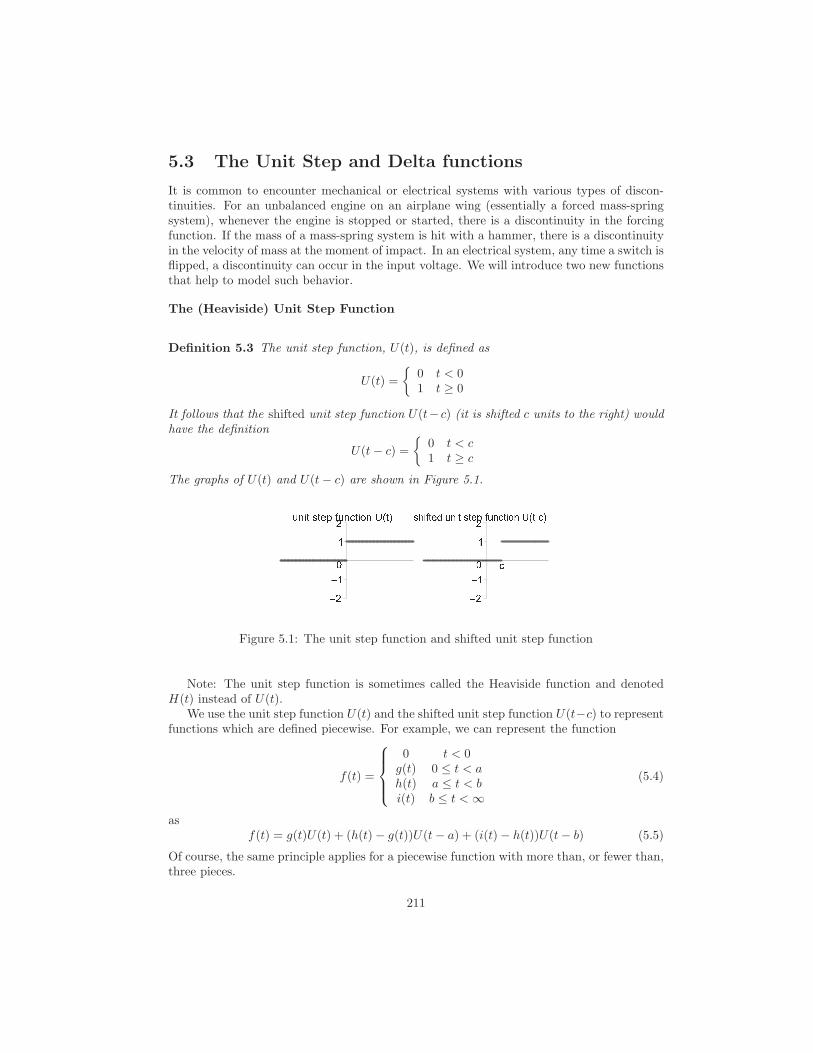
5.3 The Unit Step and Delta functions
It is common to encounter mechanical or electrical systems with various types of discon-tinuities. For an unbalanced engine on an airplane wing (essentially a forced mass-springsystem), whenever the engine is stopped or started, there is a discontinuity in the forcingfunction. If the mass of a mass-spring system is hit with a hammer, there is a discontinuityin the velocity of mass at the moment of impact. In an electrical system, any time a switch isflipped, a discontinuity can occur in the input voltage. We will introduce two new functionsthat help to model such behavior.
The (Heaviside) Unit Step Function
Definition 5.3 The unit step function, U(t), is defined as
U(t) =
{0 t < 01 t ≥ 0
It follows that the shifted unit step function U(t− c) (it is shifted c units to the right) wouldhave the definition
U(t− c) =
{0 t < c1 t ≥ c
The graphs of U(t) and U(t− c) are shown in Figure 5.1.� � � � � � � � � � � � � � � � � � � �� �� �� �� � � � ¡ ¢ £ ¤ ¥ � ¡ � ¡ ¢ ¦ ¤ ¥ § ¡ � ¨ ¥ © ª ¡ « § ¬§ ® ¯° ¯®
Figure 5.1: The unit step function and shifted unit step function
Note: The unit step function is sometimes called the Heaviside function and denotedH(t) instead of U(t).
We use the unit step function U(t) and the shifted unit step function U(t−c) to representfunctions which are defined piecewise. For example, we can represent the function
f(t) =
0 t < 0g(t) 0 ≤ t < ah(t) a ≤ t < bi(t) b ≤ t < ∞
(5.4)
asf(t) = g(t)U(t) + (h(t)− g(t))U(t− a) + (i(t)− h(t))U(t− b) (5.5)
Of course, the same principle applies for a piecewise function with more than, or fewer than,three pieces.
211
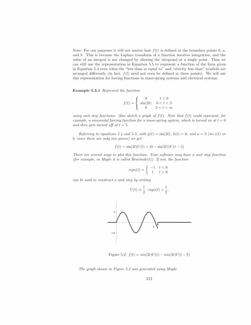
Note: For our purposes it will not matter how f(t) is defined at the boundary points 0, a,and b. This is because the Laplace transform of a function involves integration, and thevalue of an integral is not changed by altering the integrand at a single point. Thus wecan still use the representation in Equation 5.5 to represent a function of the form givenin Equation 5.4 even when the “less than or equal to” and “strictly less than” symbols arearranged differently (in fact, f(t) need not even be defined at these points). We will usethis representation for forcing functions in mass-spring systems and electrical systems.
Example 5.3.1 Represent the function
f(t) =
0 t < 0sin(2t) 0 < t < 5
0 5 < t < ∞
using unit step functions. Also sketch a graph of f(t). Note that f(t) could represent, forexample, a sinusoidal forcing function for a mass-spring system, which is turned on at t = 0and then gets turned off at t = 5.
Referring to equations 5.4 and 5.5, with g(t) = sin(2t), h(t) = 0, and a = 5 (no i(t) orb, since there are only two pieces) we get
f(t) = sin(2t)U(t) + (0− sin(2t))U(t− 5)
There are several ways to plot this function. Your software may have a unit step function(for example, in Maple it is called Heaviside(t)). If not, the function
sign(t) =
{−1 t < 01 t > 0
can be used to construct a unit step by writing
U(t) ≡ 1
2· sign(t) + 1
2.
± ² ² ³´Figure 5.2: f(t) = sin(2t)U(t)− sin(2t)U(t− 5)
The graph shown in Figure 5.2 was generated using Maple.
212
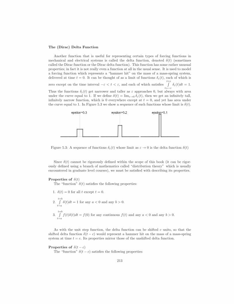
The (Dirac) Delta Function
Another function that is useful for representing certain types of forcing functions inmechanical and electrical systems is called the delta function, denoted δ(t) (sometimescalled the Dirac function or the Dirac delta function). This function has some rather unusualproperties; in fact it is not really even a function at all in the usual sense. It is used to modela forcing function which represents a “hammer hit” on the mass of a mass-spring system,delivered at time t = 0. It can be thought of as a limit of functions δε(t), each of which is
zero except on the time interval −ε < t < ε, and each of which satisfiest=ε∫
t=−ε
δε(t)dt = 1.
Thus the functions δε(t) get narrower and taller as ε approaches 0, but always with areaunder the curve equal to 1. If we define δ(t) = limε→0 δε(t), then we get an infinitely tall,infinitely narrow function, which is 0 everywhere except at t = 0, and yet has area underthe curve equal to 1. In Figure 5.3 we show a sequence of such functions whose limit is δ(t).µ ¶ · ¸ ¹ º » ¼ ½ ¾ ¿ µ ¶ · ¸ ¹ º » ¼ ½ ¾ À µ ¶ · ¸ ¹ º » ¼ ½ ¾ ÁFigure 5.3: A sequence of functions δε(t) whose limit as ε → 0 is the delta function δ(t)
Since δ(t) cannot be rigorously defined within the scope of this book (it can be rigor-ously defined using a branch of mathematics called “distribution theory” which is usuallyencountered in graduate level courses), we must be satisfied with describing its properties.
Properties of δ(t)The “function” δ(t) satisfies the following properties:
1. δ(t) = 0 for all t except t = 0.
2.t=b∫
t=a
δ(t)dt = 1 for any a < 0 and any b > 0.
3.t=b∫
t=a
f(t)δ(t)dt = f(0) for any continuous f(t) and any a < 0 and any b > 0.
As with the unit step function, the delta function can be shifted c units, so that theshifted delta function δ(t − c) would represent a hammer hit on the mass of a mass-springsystem at time t = c. Its properties mirror those of the unshifted delta function.
Properties of δ(t− c)The “function” δ(t− c) satisfies the following properties:
213
1. δ(t− c) = 0 for all t except t = c.
2.t=b∫
t=a
δ(t− c)dt = 1 for any a < c and any b > c.
3.t=b∫
t=a
f(t)δ(t− c)dt = f(c) for any continuous f(t) and any a < c and any b > c.
We provide an informal proof of Property 3, as we will need that property to find theLaplace transform of δ(t).
Proof of Property Three. If we define
δε(t) =
0 t < −ε12ε −ε ≤ t ≤ ε0 t > ε
then we get the sequence of functions pictured in Figure 5.3. Now, for any a < −ε and any
b > ε we have∫ t=b
t=aδε(t)f(t)dt =
∫ t=ε
t=−εδε(t)f(t)dt =
∫ t=ε
t=−ε12εf(t)dt =
12ε
∫ t=ε
t=−εf(t)dt. We
can represent the integral of a continuous function over an interval as its average value onthat interval, denoted favg, multiplied by the length of the interval. Thus
∫ t=ε
t=−εf(t)dt =
favg · 2ε and so∫ t=b
t=aδε(t)f(t)dt = 1
2εfavg · 2ε = favg. Now, as ε → 0, δε(t) → δ(t), andfavg → f(0) (the average value of a continuous function over a very small interval is about
equal to the value of the function at the midpoint of the interval). Thus∫ t=b
t=aδ(t)f(t)dt =
f(0). The proof that∫ t=b
t=aδ(t− c)f(t)dt = f(c) is similar.
Physical Interpretation for δ(t): The delta function will only be used in this text as partof a forcing function for a driven mass-spring system. In that context, δ(t− c) represents aunit impulse applied at time t = c. A unit impulse acting on a 1 kilogram mass increasesthe velocity instantaneously by 1 meter per second. A unit impulse acting on an m kilogrammass increases the velocity instantaneously by 1
m meters per second. Finally, N · δ(t − c)represents an impulse of N units applied at time t = c, meaning it increases the velocity ofan m kilogram mass instantaneously by N
m meters per second.
Laplace Transforms of U(t− c) and δ(t− c)In order to solve differential equations that involve U(t− c) and δ(t− c) we need to find
their Laplace transforms and add them to our list of Laplace transform formulas.
Theorem 5.5 The Laplace transforms of U(t− c) and δ(t− c) are given in the table below.
formula function Laplace transform
17 U(t− c) 1se
−sc
18 δ(t− c) e−sc
Table 6.5: Laplace transforms of U(t−c) and δ(t−c)
Proof: See the exercises at the end of this section.
214
We need one more Laplace transform formula before we can start solving differentialequations that involve U(t− c) and δ(t− c). It is one of the “general” properties that applyto any function f(t), such as the properties given in formulas 10 and 11 from Theorem 5.4.
Theorem 5.6 The Laplace transform of f(t− c)U(t− c) is given in the table below, whereF (s) is the Laplace transform of the function f(t), and c is a real constant.
formula function Laplace transform
19 f(t− c)U(t− c) e−csF (s)Table 6.6: Laplace transform of f(t−c)U(t−c)
Proof:
L[f(t− c)U(t− c)] =
∫ ∞
0
f(t− c)U(t− c)e−stdt =
∫ ∞
c
f(t− c)e−stdt;
then, substituting u = t− c,
=
∫ ∞
0
f(u)e−s(u+c)du = e−sc
∫ ∞
0
f(u)e−sudu = e−csF (s).
Note: The graph of the function f(t− c)U(t− c) is just the graph of f(t), shifted c unitsto the right, and set equal to zero up to time t = c.
Formula 19 of Theorem 5.6 is especially useful in finding the inverse Laplace transformof functions involving an exponential function e−cs.
Example 5.3.2 Use Theorem 5.6 to find L−1[
e−2s ss2+9
]
and L−1[
e−5s 4(s+1)2+16
]
.
For the first inverse Laplace transform problem, we let F (s) be ss2+9 . We should recognize
F (s) as fitting the right-hand side of formula 3 with b = 3, so we have f(t) = L−1 [F (s)] =cos(3t) (left-hand side of formula 3). The e−2s part means we need to use formula 19 withc = 2. Since f(t− 2) = cos (3(t− 2)) we have
L−1
[
e−2s s
s2 + 9
]
= L−1[e−2sF (s)
]= f(t− 2)U(t− 2)
= cos (3(t− 2))U(t− 2).
For the second inverse problem, we use F (s) = 4(s+1)2+16 , which fits the right-hand side
of formula 13 with a = −1, and b = 4; so from the left-hand side of formula 13 we getf(t) = e−1·t sin(4t). Now using formula 19 we have c = 5 (from the e−5s term), and withf(t− 5) = e−(t−5) sin (4(t− 5)) we get
L−1
[
e−5s 4
(s+ 1)2 + 9
]
= L−1[e−5sF (s)
]= f(t− 5)U(t− 5)
= e−(t−5) sin (4(t− 5))U(t− 5).
Let’s solve some differential equations!
215

Example 5.3.3 Solve the initial value problem y′′+4y = 10 sin(t− 10)U(t− 10), y(0) = 3,y′(0) = 0 using Laplace transforms. Sketch both the input (forcing function) and the responsey(t). Discuss the problem and its solution in the context of a mass-spring problem.
For the right-hand side we can use formula 19 with c = 10. Taking the Laplace transformof both sides we have
(s2Y − sy(0)− y′(0)
)+ 4Y = 10e−s·10 1
s2 + 1
so that after replacing y(0) and y′(0) with their numeric values, and isolating the Y termson the left we get
s2Y + 4Y = 10e−s·10 1
s2 + 1+ 3s
and after factoring out Y and dividing by s2 + 4 we get
Y = 10e−10s 1
(s2 + 4) (s2 + 1)+
3s
(s2 + 4).
The term 1(s2+4)(s2+1) needs to be expanded (using partial fractions):
1
(s2 + 4) (s2 + 1)=
1
3 (s2 + 1)− 1
3 (s2 + 4)
so that
Y (s) = 10e−10s
(1
3 (s2 + 1)− 1
3 (s2 + 4)
)
+3s
(s2 + 4)
=10
3e−10s 1
s2 + 1− 10
3e−10s 1
s2 + 4+ 3
s
(s2 + 4).
Taking the inverse Laplace transform of both sides yields
y(t) = L−1
[10
3e−10s 1
s2 + 1− 10
3e−10s 1
s2 + 4+ 3
s
(s2 + 4)
]
=10
3L−1
[
e−10s 1
s2 + 1
]
− 10
3· 12L−1
[
e−10s 2
s2 + 4
]
+3L−1
[s
(s2 + 4)
]
For the first two terms we combine formula 4 (letting F (s) = 1s2+1 , f(t) = sin(t) for the
first term and F (s) = 2s2+4 , f(t) = sin(2t) for the second term) with formula 19 (c = 10).
This is similar to what we did in Example 5.3.2. The third term is just formula 4 alone.We end up with
y(t) =10
3sin (t− 10)U(t− 10)− 5
3sin (2(t− 10))U(t− 10)
+3 cos(2t)
Graphs of the forcing function f(t) = 10 sin(t − 10)U(t − 10) and the response y(t) =103 sin (t− 10)U(t− 10)− 5
3 sin (2(t− 10))U(t− 10) + 3 cos 2t are shown in Figure 5.4.
216
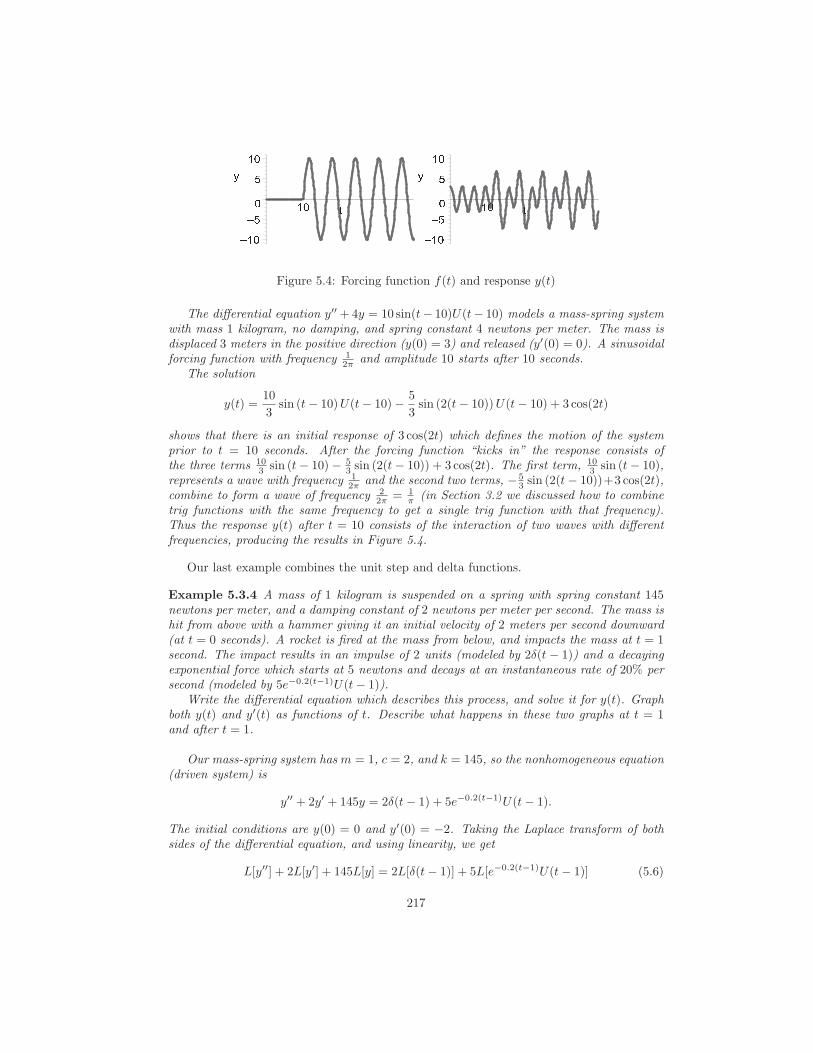
 à Ä ŠÄÅà ÄÆ Ã Ä Ç Â Ã Ä ŠÄÅà ÄÆ Ã Ä ÇFigure 5.4: Forcing function f(t) and response y(t)
The differential equation y′′ +4y = 10 sin(t− 10)U(t− 10) models a mass-spring systemwith mass 1 kilogram, no damping, and spring constant 4 newtons per meter. The mass isdisplaced 3 meters in the positive direction (y(0) = 3) and released (y′(0) = 0). A sinusoidalforcing function with frequency 1
2π and amplitude 10 starts after 10 seconds.The solution
y(t) =10
3sin (t− 10)U(t− 10)− 5
3sin (2(t− 10))U(t− 10) + 3 cos(2t)
shows that there is an initial response of 3 cos(2t) which defines the motion of the systemprior to t = 10 seconds. After the forcing function “kicks in” the response consists ofthe three terms 10
3 sin (t− 10)− 53 sin (2(t− 10)) + 3 cos(2t). The first term, 10
3 sin (t− 10),represents a wave with frequency 1
2π and the second two terms, − 53 sin (2(t− 10))+3 cos(2t),
combine to form a wave of frequency 22π = 1
π (in Section 3.2 we discussed how to combinetrig functions with the same frequency to get a single trig function with that frequency).Thus the response y(t) after t = 10 consists of the interaction of two waves with differentfrequencies, producing the results in Figure 5.4.
Our last example combines the unit step and delta functions.
Example 5.3.4 A mass of 1 kilogram is suspended on a spring with spring constant 145newtons per meter, and a damping constant of 2 newtons per meter per second. The mass ishit from above with a hammer giving it an initial velocity of 2 meters per second downward(at t = 0 seconds). A rocket is fired at the mass from below, and impacts the mass at t = 1second. The impact results in an impulse of 2 units (modeled by 2δ(t − 1)) and a decayingexponential force which starts at 5 newtons and decays at an instantaneous rate of 20% persecond (modeled by 5e−0.2(t−1)U(t− 1)).
Write the differential equation which describes this process, and solve it for y(t). Graphboth y(t) and y′(t) as functions of t. Describe what happens in these two graphs at t = 1and after t = 1.
Our mass-spring system has m = 1, c = 2, and k = 145, so the nonhomogeneous equation(driven system) is
y′′ + 2y′ + 145y = 2δ(t− 1) + 5e−0.2(t−1)U(t− 1).
The initial conditions are y(0) = 0 and y′(0) = −2. Taking the Laplace transform of bothsides of the differential equation, and using linearity, we get
L[y′′] + 2L[y′] + 145L[y] = 2L[δ(t− 1)] + 5L[e−0.2(t−1)U(t− 1)] (5.6)
217
Using formulas 8 and 9 from section 5.1 for the left-hand side of equation 5.6, and Table 6.5for the first term on the right-hand side, and Table 6.6 (with f(t) = e−0.2t, F (s) = 1
s+0.2 ,c = 1) for the second term on the right-hand side we get
(s2Y − s · 0− (−2)
)+ 2(sY − 0) + 145Y = 2e−(1)s + 5
(
e−1·s 1
s+ 0.2
)
Now collect Y terms on the left and factor out Y :
(s2 + 2s+ 145
)Y = −2 + 2e−s + 5e−s 1
s+ 0.2
and then divide by s2 + 2s+ 145 to get
Y = −21
s2 + 2s+ 145+ 2e−s 1
s2 + 2s+ 145+ 5e−s 1
(s2 + 2s+ 145) (s+ 0.2)(5.7)
For the first two terms in equation 5.7 we complete the square in the denominator
s2 + 2s+ 145 = s2 + 2s+ 1− 1 + 145 = (s+ 1)2 + 144
and for the last term in equation (5.7) we use partial fractions first, and then completethe square (turning decimal numbers into fractions is often helpful when using computeralgebra):
1
(s2 + 2s+ 145)(s+ 1
5
)
=
(1
3616
)
·(
125
5s+ 1
)
+
(1
3616
)
·( −25s− 45
2s+ s2 + 145
)
=
(1
3616
)
·(1
5
)
·(
125
s+ 15
)
+
(1
3616
)
·( −25s− 45
(s+ 1)2 + 144
)
Equation (5.7) now becomes
Y = −21
(s+ 1)2 + 144+ 2e−s 1
(s+ 1)2 + 144
+5e−s
((1
3616
)
·(1
5
)
·(
125
s+ 15
)
+
(1
3616
)
·( −25s− 45
(s+ 1)2 + 144
))
= − 2
12· 12
(s+ 1)2 + 144+
2
12· e−s 12
(s+ 1)2 + 144
+125
3616· e−s 1
s+ 15
+5
3616· e−s −25s− 45
(s+ 1)2 + 144(5.8)
after multiplying out and using the standard “multiply and divide” trick on the first twoterms. The first three terms are now set up for the inverse Laplace transformation, but thelast needs some work. We need to split it up and use the “add and subtract” trick:
−25s− 45
(s+ 1)2 + 144= −25
s+ 1− 1
(s+ 1)2 + 144− 45
1
(s+ 1)2 + 144
= −25s+ 1
(s+ 1)2 + 144+ 25
1
(s+ 1)2 + 144− 45
1
(s+ 1)2 + 144
= −25s+ 1
(s+ 1)2 + 144− 20
12· 12
(s+ 1)2 + 144
218
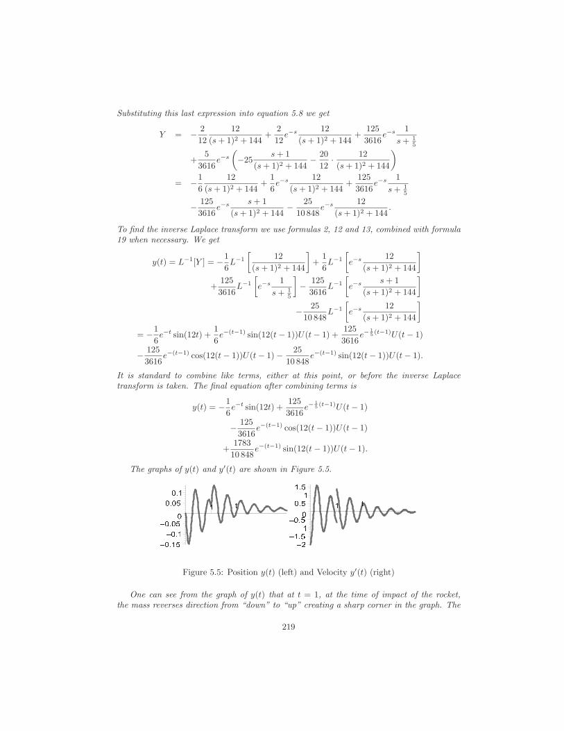
Substituting this last expression into equation 5.8 we get
Y = − 2
12
12
(s+ 1)2 + 144+
2
12e−s 12
(s+ 1)2 + 144+
125
3616e−s 1
s+ 15
+5
3616e−s
(
−25s+ 1
(s+ 1)2 + 144− 20
12· 12
(s+ 1)2 + 144
)
= −1
6
12
(s+ 1)2 + 144+
1
6e−s 12
(s+ 1)2 + 144+
125
3616e−s 1
s+ 15
− 125
3616e−s s+ 1
(s+ 1)2 + 144− 25
10 848e−s 12
(s+ 1)2 + 144.
To find the inverse Laplace transform we use formulas 2, 12 and 13, combined with formula19 when necessary. We get
y(t) = L−1[Y ] = −1
6L−1
[12
(s+ 1)2 + 144
]
+1
6L−1
[
e−s 12
(s+ 1)2 + 144
]
+125
3616L−1
[
e−s 1
s+ 15
]
− 125
3616L−1
[
e−s s+ 1
(s+ 1)2 + 144
]
− 25
10 848L−1
[
e−s 12
(s+ 1)2 + 144
]
= −1
6e−t sin(12t) +
1
6e−(t−1) sin(12(t− 1))U(t− 1) +
125
3616e−
15(t−1)U(t− 1)
− 125
3616e−(t−1) cos(12(t− 1))U(t− 1)− 25
10 848e−(t−1) sin(12(t− 1))U(t− 1).
It is standard to combine like terms, either at this point, or before the inverse Laplacetransform is taken. The final equation after combining terms is
y(t) = −1
6e−t sin(12t) +
125
3616e−
15(t−1)U(t− 1)
− 125
3616e−(t−1) cos(12(t− 1))U(t− 1)
+1783
10 848e−(t−1) sin(12(t− 1))U(t− 1).
The graphs of y(t) and y′(t) are shown in Figure 5.5.
È É Ê Ë ÌÈ É Ê ËÈ É Ê É Ì ÉÉ Ê É ÌÉ Ê Ë Ë Í Î ÏÎ Ð Ñ ÒÎ ÐÎ Ó Ñ Ò ÓÓ Ñ Ò ÐÐ Ñ Ò Ð ÔFigure 5.5: Position y(t) (left) and Velocity y′(t) (right)
One can see from the graph of y(t) that at t = 1, at the time of impact of the rocket,the mass reverses direction from “down” to “up” creating a sharp corner in the graph. The
219
graph of y′(t) shows a discontinuity at this point, flipping instantaneously from negative topositive. After t = 1, the rocket continues to fire, but with exponentially decreasing force.This causes the oscillations to become raised (they are no longer centered on y = 0), but thecenter of the oscillations is gradually coming back down towards y = 0 as the rocket forcedies out.
We conclude this section with a list of all the Laplace transform formulas that we havedeveloped up to this point.
220
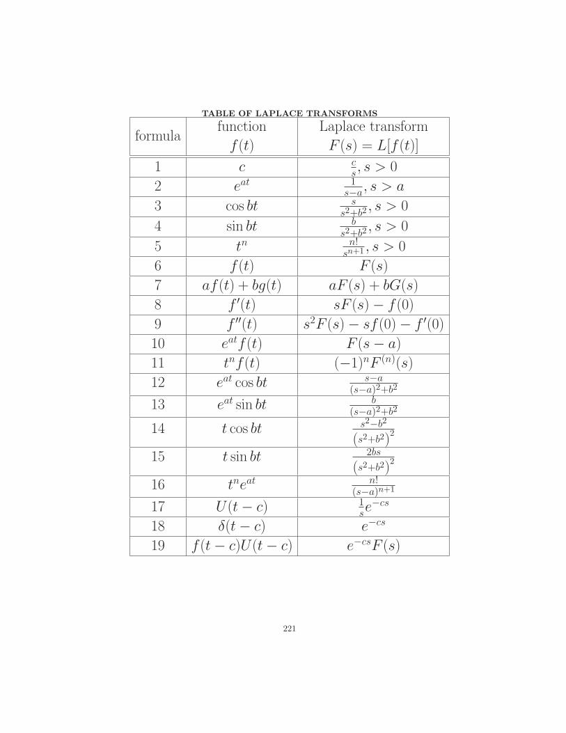
TABLE OF LAPLACE TRANSFORMS
formulafunction
f (t)
Laplace transform
F (s) = L[f (t)]
1 c cs, s > 0
2 eat 1s−a
, s > a
3 cos bt ss2+b2
, s > 0
4 sin bt bs2+b2
, s > 0
5 tn n!sn+1 , s > 0
6 f (t) F (s)
7 af (t) + bg(t) aF (s) + bG(s)
8 f ′(t) sF (s)− f (0)
9 f ′′(t) s2F (s)− sf (0)− f ′(0)10 eatf (t) F (s− a)
11 tnf (t) (−1)nF (n)(s)
12 eat cos bt s−a(s−a)2+b2
13 eat sin bt b(s−a)2+b2
14 t cos bt s2−b2
(s2+b2)2
15 t sin bt 2bs
(s2+b2)2
16 tneat n!(s−a)n+1
17 U(t− c) 1se−cs
18 δ(t− c) e−cs
19 f (t− c)U(t− c) e−csF (s)
221
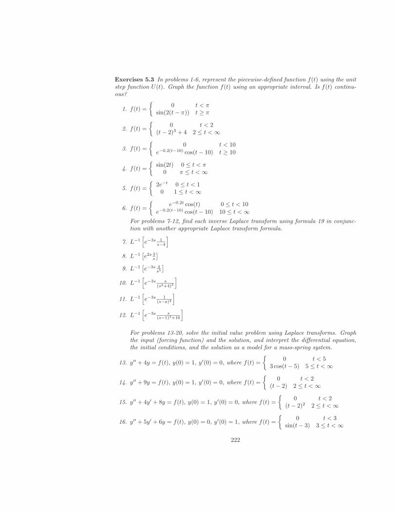
Exercises 5.3 In problems 1-6, represent the piecewise-defined function f(t) using the unitstep function U(t). Graph the function f(t) using an appropriate interval. Is f(t) continu-ous?
1. f(t) =
{0 t < π
sin(2(t− π)) t ≥ π
2. f(t) =
{0 t < 2
(t− 2)3 + 4 2 ≤ t < ∞
3. f(t) =
{0 t < 10
e−0.2(t−10) cos(t− 10) t ≥ 10
4. f(t) =
{sin(2t) 0 ≤ t < π
0 π ≤ t < ∞
5. f(t) =
{2e−t 0 ≤ t < 10 1 ≤ t < ∞
6. f(t) =
{e−0.2t cos(t) 0 ≤ t < 10
e−0.2(t−10) cos(t− 10) 10 ≤ t < ∞For problems 7-12, find each inverse Laplace transform using formula 19 in conjunc-tion with another appropriate Laplace transform formula.
7. L−1[
e−3s 1s−4
]
8. L−1[e2s 3
s
]
9. L−1[e−3s 4
s5
]
10. L−1[
e−3s s(s2+4)2
]
11. L−1[
e−3s 1(s−a)4
]
12. L−1[
e−3s s(s−1)2+16
]
For problems 13-20, solve the initial value problem using Laplace transforms. Graphthe input (forcing function) and the solution, and interpret the differential equation,the initial conditions, and the solution as a model for a mass-spring system.
13. y′′ + 4y = f(t), y(0) = 1, y′(0) = 0, where f(t) =
{0 t < 5
3 cos(t− 5) 5 ≤ t < ∞
14. y′′ + 9y = f(t), y(0) = 1, y′(0) = 0, where f(t) =
{0 t < 2
(t− 2) 2 ≤ t < ∞
15. y′′ + 4y′ + 8y = f(t), y(0) = 1, y′(0) = 0, where f(t) =
{0 t < 2
(t− 2)2 2 ≤ t < ∞
16. y′′ + 5y′ + 6y = f(t), y(0) = 0, y′(0) = 1, where f(t) =
{0 t < 3
sin(t− 3) 3 ≤ t < ∞
222
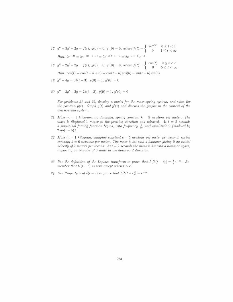
17. y′′ + 3y′ + 2y = f(t), y(0) = 0, y′(0) = 0, where f(t) =
{2e−3t 0 ≤ t < 10 1 ≤ t < ∞
Hint: 2e−3t = 2e−3(t−1+1) = 2e−3(t−1)−3 = 2e−3(t−1)e−3
18. y′′ + 2y′ + 2y = f(t), y(0) = 0, y′(0) = 0, where f(t) =
{cos(t) 0 ≤ t < 50 5 ≤ t < ∞
Hint: cos(t) = cos(t− 5 + 5) = cos(t− 5) cos(5)− sin(t− 5) sin(5)
19. y′′ + 4y = 3δ(t− 3), y(0) = 1, y′(0) = 0
20. y′′ + 3y′ + 2y = 2δ(t− 3), y(0) = 1, y′(0) = 0
For problems 21 and 22, develop a model for the mass-spring system, and solve forthe position y(t). Graph y(t) and y′(t) and discuss the graphs in the context of themass-spring system.
21. Mass m = 1 kilogram, no damping, spring constant k = 9 newtons per meter. Themass is displaced 1 meter in the positive direction and released. At t = 5 secondsa sinusoidal forcing function begins, with frequency 1
2π and amplitude 2 (modeled by2 sin(t− 5)).
22. Mass m = 1 kilogram, damping constant c = 5 newtons per meter per second, springconstant k = 6 newtons per meter. The mass is hit with a hammer giving it an initialvelocity of 2 meters per second. At t = 2 seconds the mass is hit with a hammer again,imparting an impulse of 3 units in the downward direction.
23. Use the definition of the Laplace transform to prove that L[U(t − c)] = 1se
−sc. Re-member that U(t− c) is zero except when t > c.
24. Use Property 3 of δ(t− c) to prove that L[δ(t− c)] = e−sc.
223
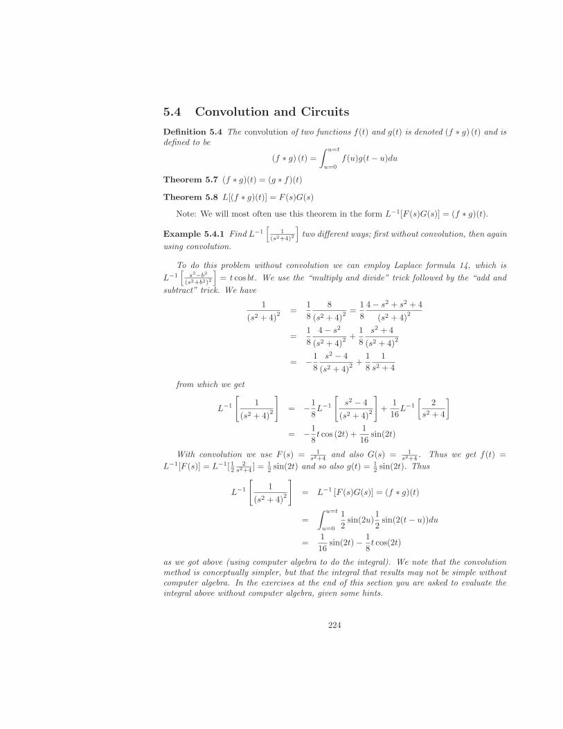
5.4 Convolution and Circuits
Definition 5.4 The convolution of two functions f(t) and g(t) is denoted (f ∗ g) (t) and isdefined to be
(f ∗ g) (t) =∫ u=t
u=0
f(u)g(t− u)du
Theorem 5.7 (f ∗ g)(t) = (g ∗ f)(t)
Theorem 5.8 L[(f ∗ g)(t)] = F (s)G(s)
Note: We will most often use this theorem in the form L−1[F (s)G(s)] = (f ∗ g)(t).
Example 5.4.1 Find L−1[
1(s2+4)2
]
two different ways; first without convolution, then again
using convolution.
To do this problem without convolution we can employ Laplace formula 14, which is
L−1[
s2−b2
(s2+b2)2
]
= t cos bt. We use the “multiply and divide” trick followed by the “add and
subtract” trick. We have
1
(s2 + 4)2 =
1
8
8
(s2 + 4)2 =
1
8
4− s2 + s2 + 4
(s2 + 4)2
=1
8
4− s2
(s2 + 4)2 +
1
8
s2 + 4
(s2 + 4)2
= −1
8
s2 − 4
(s2 + 4)2 +
1
8
1
s2 + 4
from which we get
L−1
[
1
(s2 + 4)2
]
= −1
8L−1
[
s2 − 4
(s2 + 4)2
]
+1
16L−1
[2
s2 + 4
]
= −1
8t cos (2t) +
1
16sin(2t)
With convolution we use F (s) = 1s2+4 and also G(s) = 1
s2+4 . Thus we get f(t) =
L−1[F (s)] = L−1[ 122
s2+4 ] =12 sin(2t) and so also g(t) = 1
2 sin(2t). Thus
L−1
[
1
(s2 + 4)2
]
= L−1 [F (s)G(s)] = (f ∗ g)(t)
=
∫ u=t
u=0
1
2sin(2u)
1
2sin(2(t− u))du
=1
16sin(2t)− 1
8t cos(2t)
as we got above (using computer algebra to do the integral). We note that the convolutionmethod is conceptually simpler, but that the integral that results may not be simple withoutcomputer algebra. In the exercises at the end of this section you are asked to evaluate theintegral above without computer algebra, given some hints.
224
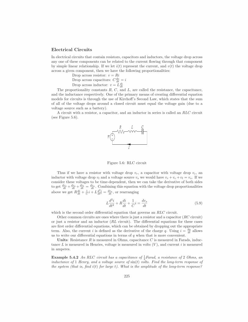
Electrical Circuits
In electrical circuits that contain resistors, capacitors and inductors, the voltage drop acrossany one of these components can be related to the current flowing through that componentby simple linear relationship. If we let i(t) represent the current, and v(t) the voltage dropacross a given component, then we have the following proportionalities:
Drop across resistor: v = RiDrop across capacitors: C dv
dt = i
Drop across inductor: v = L didt
The proportionality constants R, C, and L, are called the resistance, the capacitance,and the inductance respectively. One of the primary means of creating differential equationmodels for circuits is through the use of Kirchoff’s Second Law, which states that the sumof all of the voltage drops around a closed circuit must equal the voltage gain (due to avoltage source such as a battery).
A circuit with a resistor, a capacitor, and an inductor in series is called an RLC circuit(see Figure 5.6).
Figure 5.6: RLC circuit
Thus if we have a resistor with voltage drop vr, a capacitor with voltage drop vc, aninductor with voltage drop vl and a voltage source vs we would have vr + vc+ vl = vs. If weconsider these voltages to be time-dependent, then we can take the derivative of both sidesto get dvr
dt + dvcdt + dvl
dt = dvsdt . Combining this equation with the voltage drop proportionalities
above we get R didt +
1C i+ L d2i
dt2 = dvsdt , or rearranging
Ld2i
dt2+R
di
dt+
1
Ci =
dvsdt
(5.9)
which is the second order differential equation that governs an RLC circuit.Other common circuits are ones where there is just a resistor and a capacitor (RC circuit)
or just a resistor and an inductor (RL circuit). The differential equations for these casesare first order differential equations, which can be obtained by dropping out the appropriateterm. Also, the current i is defined as the derivative of the charge q. Using i = dq
dt allowsus to write our differential equations in terms of q when that is more convenient.
Units: Resistance R is measured in Ohms, capacitance C is measured in Farads, induc-tance L is measured in Henries, voltage is measured in volts (V ), and current i is measuredin amperes.
Example 5.4.2 An RLC circuit has a capacitance of 12Farad, a resistance of 2 Ohms, an
inductance of 1 Henry, and a voltage source of sin(t) volts. Find the long-term response ofthe system (that is, find i(t) for large t). What is the amplitude of the long-term response?
225
We have C = 12 , R = 2, L = 1, and vs = sin(t) and hence dvs
dt = cos(t). Employingequation 5.9 we get
d2i
dt2+ 2
di
dt+ 2i = cos(t). (5.10)
Even though we are going to employ Laplace transforms to solve this differential equation,we will first use the techniques of Chapter 3 to observe that the characteristic equation isr2 + 2r + 2 = 0, which has solutions r = −1 ± i. Thus the homogeneous solution would beih = C1e
−t cos t + C2e−t sin t. As t → ∞ we have ih → 0, so that the long-term response
consists of only the particular solution ip. An important consequence of this fact is that theinitial conditions i(0) and i′(0) have no affect on the long term behavior of the system. Henceto make the algebra of Laplace transforms simpler, we can assume i(0) = 0 and i′(0) = 0.
Taking the transform of both sides of equation 5.10 we get
s2I(s) + 2sI(s) + 2I(s) =s
s2 + 1
and then solving for I(s) we get
I(s) =s
s2 + 1
1
s2 + 2s+ 2. (5.11)
At this point we could use the techniques of Sections 6.1 and 6.2 (expand, complete thesquare), but instead we choose convolution. With F (s) = s
s2+1 and G(s) = 1s2+2s+2 =
1(s+1)2+1
we have f(t) = cos t and g(t) = e−t sin t. Thus
i(t) = (f ∗ g)(t) = (g ∗ f)(t) =∫ u=t
u=0
g(u)f(t− u)du
=
∫ u=t
u=0
(e−u sinu
)cos(t− u)du
=1
5cos(t) +
2
5sin(t)− 1
5e−t cos t− 3
5e−t sin t,
using computer algebra to do the integral. Thus the long-term response would be given by
ip =1
5cos(t) +
2
5sin(t).
Finally, we can combine sine and cosine terms as shown in Section 3.3:
ip(t) =2
5sin(t) +
1
5cos(t) = D cos(t− φ).
We have D2 =(25
)2+
(15
)2= 1
5 and tan(φ) = 2/51/5 = 2. With D =
√15 we must choose
φ = arctan(2) ≈ 0.352π (show why φ = arctan(2) + π does not work). Thus
ip(t) ≈√
1
5cos(t− 0. 352π).
The amplitude of the long-term response is√
15 ≈ 0.447 21.
An important concept that we need to take away from Example 5.4.2 is that wheneverthere is non-zero resistance in an RLC circuit, and we are only interested in the long-termoutput, we can set the initial conditions to zero. We will take that course for the rest ofthis section.
226

Transfer Functions and the Frequency Domain
Equation 5.11 from Example 5.4.2 provides another important concept that we can apply ingeneral to electrical circuits (and mechanical systems as well) for which the initial conditionsare zero. When we solve an initial value problem of the form ay′ + by = f(t), y(0) = 0(first-order linear) or of the form ay′′ + by′ + cy = f(t), y(0) = 0, y′(0) = 0 (second-orderlinear), we interpret the function f(t) as the input and the solution y(t) as the output (orthe response).
Definition 5.5 For a nonhomogeneous linear differential equation with input (forcing func-tion) f(t) and output (solution) y(t), and zero initial conditions, the ratio of the Laplacetransform of the output Y (s) to the Laplace transform of the input F (s) is called the transfer
function. We will denote the transfer function by H(s) = Y (s)F (s) .
Since Y (s) = H(s)F (s), we have y(t) = L−1[Y (s)] = L−1[H(s)F (s)] = (h ∗ f)(t). Bothy and f are functions of t (time), hence when we deal with these functions we say that weare working in the time domain. The functions Y and F are functions of s, so that when wework with these functions we say we are working in the frequency domain (also called thes− plane). Because multiplication is a simpler operation than convolution, many electricalengineers prefer working in the frequency domain.
In Example 5.4.2, the input is f(t) = cos t and the Laplace transform of the input isF (s) = s
s2+1 .The Laplace transform of the output is I(s). From equation 5.11, we see that
the transfer function for that example is given by H(s) = I(s)F (s) =
1s2+2s+2 .
Example 5.4.3 An RLC circuit has in input given by F (s) = 5 ss2+9 and transfer function
given by H(s) = 1s2+2s+5 . Find the output in both the frequency domain (that is Y (s)) and in
the time domain (that is y(t)), and find the long-term amplitude in the time domain. Also,find the initial value problem (differential equation plus initial conditions) corresponding tothe given input and transfer function, and state the capacitance, resistance, and inductanceof the circuit.
The output in the frequency domain is just the product of the input and the transferfunction, thus
Y (s) = H(s)F (s) =1
s2 + 2s+ 5· 5 s
s2 + 9.
To find the output in the time domain we use convolution, along with computer algebra toevaluate the integral. First we need to transform F (s) and H(s) to the time domain. Wehave
f(t) = L−1[F (s)] = L−1
[
5s
s2 + 9
]
= 5 cos(3t)
and
h(t) = L−1[H(s)] = L−1
[1
s2 + 2s+ 5
]
= L−1
[1
s2 + 2s+ 1 + 4
]
= L−1
[
1
(s+ 1)2+ 4
]
= L−1
[
1
2
2
(s+ 1)2+ 4
]
=1
2e−t sin(2t).
227
Thus
y(t) = L−1[Y (s)] = L−1 [H(s)F (s)] = (h ∗ f)(t) =∫ u=t
u=0
h(t− u)f(u)du
=
∫ t
0
1
2e−(t−u) sin(2(t− u)) · 5 cos(3u)du
=15
26sin 3t− 5
13cos 3t+
5
13(cos 2t) e−t − 35
52(sin 2t) e−t
(Note : The form of y(t) will vary between different computer algebra systems).
In the long term (that is, as t → ∞), y(t) approaches the steady-state solution 1526 sin 3t −
513 cos 3t. The amplitude of the steady-state solution would be
√(1526
)2+(
513
)2= 5
26
√13 ≈
0.693 38.To determine the differential equation, we write the equation Y (s) = H(s)F (s) as
Y (s) 1H(s) = F (s) which becomes
Y (s)(s2 + 2s+ 5) = 5s
s2 + 9
or equivalently
s2Y (s) + 2sY (s) + 5Y (s) = 5s
s2 + 9.
We can see that the above equation is the result of taking the Laplce transform of both sidesof the differential equation
y′′(t) + 2y′(t) + 5y(t) = 5 cos(3t)
if we take the initial conditions to be y(0) = 0 and y′(0) = 0 (check this). Thus L = 1Henry, R = 2 Ohms, and C = 1
5 Farads.
Filters and the Response Curve
One of the points of Example 5.4.3 is that all of the important information about a circuitis contained in the transfer function H(s) and the input F (s). If the input is not specified,then the transfer function tells the whole story; it specifies how to get from the input to theoutput (in either the time or frequency domain).
One important property of an electrical circuit is how the frequency of the input affectsthe amplitude of the output (in the long term). In Example 5.4.3, the frequency of the inputwas 3
2π and the amplitude of the output was about 0.693. The graph of amplitude of theoutput (long term) as a function of the input frequency is referred to as the response curveof the system.
Example 5.4.4 Consider an RLC circuit, with resistance 2 Ohms, capacitance 15Farads,
and inductance 1 Henry (this is the same circuit as in Example 5.4.3). Find the (longterm) output amplitude as a function of the parameter ω if the input is given by the forcingfunction f(t) = 5 cos(ωt), and graph this function. Also, determine the value of ω that hasthe largest ouput amplitude. (Note: ω is related to the frequency f by the formula f = ω
2π
228
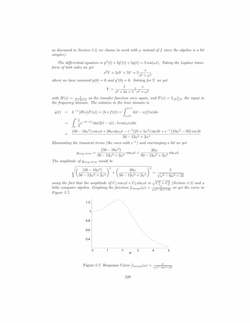
as discussed in Section 3.2; we choose to work with ω instead of f since the algebra is a bitsimpler).
The differential equation is y′′(t) + 2y′(t) + 5y(t) = 5 cos(ωt). Taking the Laplace trans-form of both sides we get
s2Y + 2sY + 5Y = 5s
s2 + ω2
where we have assumed y(0) = 0 and y′(0) = 0. Solving for Y we get
Y =1
s2 + 2s+ 55
s
s2 + ω2
with H(s) = 1s2+2s+5 as the transfer function once again, and F (s) = 5 s
s2+ω2 the input inthe frequency domain. The solution in the time domain is
y(t) = L−1 [H(s)F (s)] = (h ∗ f)(t) =∫ u=t
u=0
h(t− u)f(u)du
=
∫ t
0
1
2e−(t−u) sin(2(t− u)) · 5 cos(ωu)du
=(50− 10ω2) cosωt+ 20ω sinωt− e−t(25 + 5ω2) sin 2t+ e−t
(10ω2 − 50
)cos 2t
50− 12ω2 + 2ω4
Eliminating the transient terms (the ones with e−t) and rearranging a bit we get
ylong term =
(50− 10ω2
)
50− 12ω2 + 2ω4cosωt+
20ω
50− 12ω2 + 2ω4sinωt.
The amplitude of ylong term would be√(
(50− 10ω2)
50− 12ω2 + 2ω4
)2
+
(20ω
50− 12ω2 + 2ω4
)2
=5√
ω4 − 6ω2 + 25
using the fact that the amplitude of C1 cosωt + C2 sinωt is√
C21 + C2
2 (Section 3.3) and alittle computer algebra. Graphing the function fomega(ω) =
5√ω4−6ω2+25
we get the curve in
Figure 5.7.
Õ Ö ×Õ Ö ØÕ Ö Ù ÚÚ Ö ÛÕ Ú Û Ü × ÝÞ
Figure 5.7: Response Curve fomega(ω) =5√
ω4−6ω2+25
229
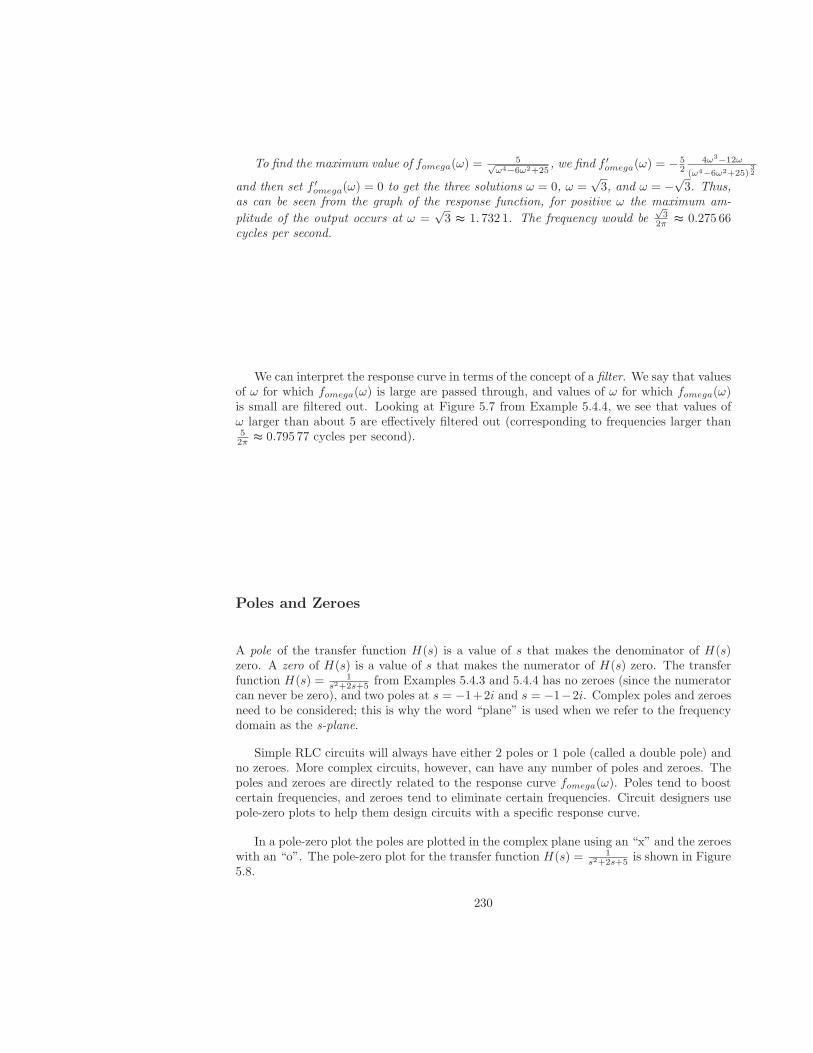
To find the maximum value of fomega(ω) =5√
ω4−6ω2+25, we find f ′
omega(ω) = − 52
4ω3−12ω
(ω4−6ω2+25)32
and then set f ′omega(ω) = 0 to get the three solutions ω = 0, ω =
√3, and ω = −
√3. Thus,
as can be seen from the graph of the response function, for positive ω the maximum am-
plitude of the output occurs at ω =√3 ≈ 1. 732 1. The frequency would be
√3
2π ≈ 0.275 66cycles per second.
We can interpret the response curve in terms of the concept of a filter. We say that valuesof ω for which fomega(ω) is large are passed through, and values of ω for which fomega(ω)is small are filtered out. Looking at Figure 5.7 from Example 5.4.4, we see that values ofω larger than about 5 are effectively filtered out (corresponding to frequencies larger than52π ≈ 0.795 77 cycles per second).
Poles and Zeroes
A pole of the transfer function H(s) is a value of s that makes the denominator of H(s)zero. A zero of H(s) is a value of s that makes the numerator of H(s) zero. The transferfunction H(s) = 1
s2+2s+5 from Examples 5.4.3 and 5.4.4 has no zeroes (since the numeratorcan never be zero), and two poles at s = −1+2i and s = −1−2i. Complex poles and zeroesneed to be considered; this is why the word “plane” is used when we refer to the frequencydomain as the s-plane.
Simple RLC circuits will always have either 2 poles or 1 pole (called a double pole) andno zeroes. More complex circuits, however, can have any number of poles and zeroes. Thepoles and zeroes are directly related to the response curve fomega(ω). Poles tend to boostcertain frequencies, and zeroes tend to eliminate certain frequencies. Circuit designers usepole-zero plots to help them design circuits with a specific response curve.
In a pole-zero plot the poles are plotted in the complex plane using an “x” and the zeroeswith an “o”. The pole-zero plot for the transfer function H(s) = 1
s2+2s+5 is shown in Figure5.8.
230
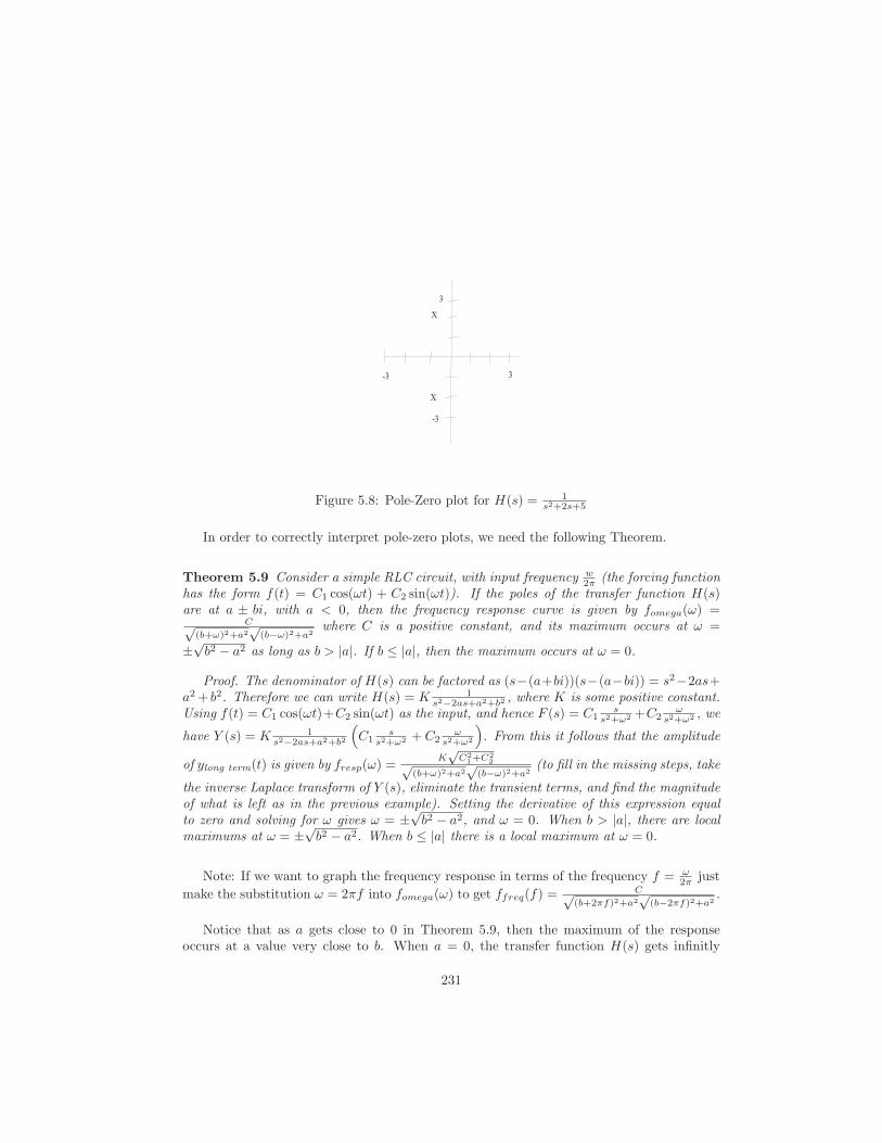
Figure 5.8: Pole-Zero plot for H(s) = 1s2+2s+5
In order to correctly interpret pole-zero plots, we need the following Theorem.
Theorem 5.9 Consider a simple RLC circuit, with input frequency w2π (the forcing function
has the form f(t) = C1 cos(ωt) + C2 sin(ωt)). If the poles of the transfer function H(s)are at a ± bi, with a < 0, then the frequency response curve is given by fomega(ω) =
C√(b+ω)2+a2
√(b−ω)2+a2
where C is a positive constant, and its maximum occurs at ω =
±√b2 − a2 as long as b > |a|. If b ≤ |a|, then the maximum occurs at ω = 0.
Proof. The denominator of H(s) can be factored as (s−(a+bi))(s−(a−bi)) = s2−2as+a2+ b2. Therefore we can write H(s) = K 1
s2−2as+a2+b2 , where K is some positive constant.Using f(t) = C1 cos(ωt)+C2 sin(ωt) as the input, and hence F (s) = C1
ss2+ω2 +C2
ωs2+ω2 , we
have Y (s) = K 1s2−2as+a2+b2
(
C1s
s2+ω2 + C2ω
s2+ω2
)
. From this it follows that the amplitude
of ylong term(t) is given by fresp(ω) =K√
C21+C2
2√(b+ω)2+a2
√(b−ω)2+a2
(to fill in the missing steps, take
the inverse Laplace transform of Y (s), eliminate the transient terms, and find the magnitudeof what is left as in the previous example). Setting the derivative of this expression equalto zero and solving for ω gives ω = ±
√b2 − a2, and ω = 0. When b > |a|, there are local
maximums at ω = ±√b2 − a2. When b ≤ |a| there is a local maximum at ω = 0.
Note: If we want to graph the frequency response in terms of the frequency f = ω2π just
make the substitution ω = 2πf into fomega(ω) to get ffreq(f) =C√
(b+2πf)2+a2√
(b−2πf)2+a2.
Notice that as a gets close to 0 in Theorem 5.9, then the maximum of the responseoccurs at a value very close to b. When a = 0, the transfer function H(s) gets infinitly
231
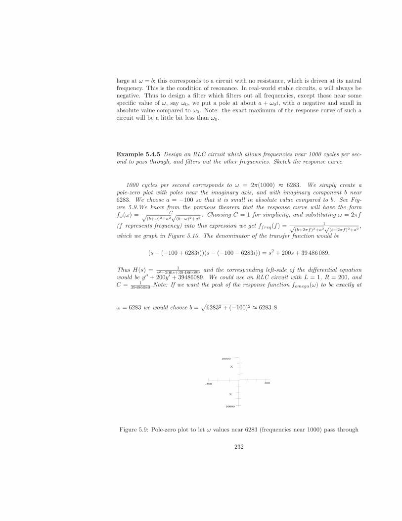
large at ω = b; this corresponds to a circuit with no resistance, which is driven at its natralfrequency. This is the condition of resonance. In real-world stable circuits, a will always benegative. Thus to design a filter which filters out all frequencies, except those near somespecific value of ω, say ω0, we put a pole at about a + ω0i, with a negative and small inabsolute value compared to ω0. Note: the exact maximum of the response curve of such acircuit will be a little bit less than ω0.
Example 5.4.5 Design an RLC circuit which allows frequencies near 1000 cycles per sec-ond to pass through, and filters out the other frequencies. Sketch the response curve.
1000 cycles per second corresponds to ω = 2π(1000) ≈ 6283. We simply create apole-zero plot with poles near the imaginary axis, and with imaginary component b near6283. We choose a = −100 so that it is small in absolute value compared to b. See Fig-ure 5.9.We know from the previous theorem that the response curve will have the formfω(ω) =
C√(b+ω)2+a2
√(b−ω)2+a2
. Choosing C = 1 for simplicity, and substituting ω = 2πf
(f represents frequency) into this expression we get ffreq(f) =1√
(b+2πf)2+a2√
(b−2πf)2+a2,
which we graph in Figure 5.10. The denominator of the transfer function would be
(s− (−100 + 6283i))(s− (−100− 6283i)) = s2 + 200s+ 39 486 089.
Thus H(s) = 1s2+200s+39 486 089 and the corresponding left-side of the differential equation
would be y′′ + 200y′ + 39486089. We could use an RLC circuit with L = 1, R = 200, andC = 1
39486089 .Note: If we want the peak of the response function fomega(ω) to be exactly at
ω = 6283 we would choose b =√
62832 + (−100)2 ≈ 6283. 8.
Figure 5.9: Pole-zero plot to let ω values near 6283 (frequencies near 1000) pass through
232
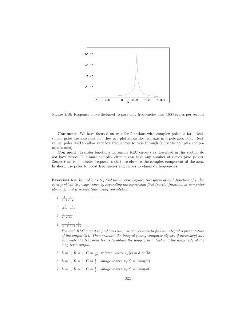
ß à á â ãä à á â ãå à á â ãæ à á â ãâ ß â â â ä â â â å â â â æ â â â ç â â â âè
Figure 5.10: Response curve designed to pass only frequencies near 1000 cycles per second
Comment: We have focused on transfer functions with complex poles so far. Real-valued poles are also possible: they are plotted on the real axis in a pole-zero plot. Real-valued poles tend to allow very low frequencies to pass through (since the complex compo-nent is zero).
Comment: Transfer functions for simple RLC circuits as described in this section donot have zeroes, but more complex circuits can have any number of zeroes (and poles).Zeroes tend to eliminate frequencies that are close to the complex component of the zero.In short, use poles to boost frequencies and zeroes to eliminate frequencies.
Exercises 5.4 In problems 1-4 find the inverse Laplace transform of each function of s. Doeach problem two ways; once by expanding the expression first (partial fractions or computeralgebra), and a second time using convolution.
1. 1s−1
1s−2
2. ss2+1
1s+3
3. 1s2
1s2+4
4. 5(s−1)2+4
2s+7
For each RLC circuit in problems 5-8, use convolution to find an integral representationof the output i(t). Then evaluate the integral (using computer algebra if necessary) andeliminate the transient terms to obtain the long-term output and the amplitude of thelong-term output.
5. L = 1, R = 4, C = 129 , voltage source vs(t) = 3 sin(5t).
6. L = 1, R = 3, C = 12 , voltage source vs(t) = 3 sin(5t).
7. L = 1, R = 3, C = 12 , voltage source vs(t) = 3 sin(ωt).
233
8. L = 1, R = 4, C = 129 , voltage source vs(t) = 3 sin(ωt).
Find the long-term output i(t) in the time domain, and find and sketch the responsecurve fomega(ω), given the transfer function H(s) and input F (s) in the frequencydomain. Also give the corresponding differential equation.
9. H(s) = 1s2+2s+10 , F (s) = s
s2+ω2 .
10. H(s) = 1s2+4s+13 , F (s) = ω
s2+ω2 .
Use a pole-zero plot to design an RLC circuit which filters out all frequencies exceptthose near the given frequency f . Then design a second filter which has a wider pass-band (the response curve is wider), centered at roughly the same frequency f as thefirst filter. Give the values of R, L, and C for each case.
11. Frequency f = 15000 cycles per second.
12. Frequency f = 0 cycles per second.
13. Evaluate the convolution integral∫ u=t
u=012 sin(2u)
12 sin(2(t − u))du without using com-
puter algebra. You will need to use the trig identities sin(A ± B) = sin(A) cos(B) ±cos(A) sin(B) and cos(A±B) = cos(A) cos(B)∓ sin(A) sin(B).
234
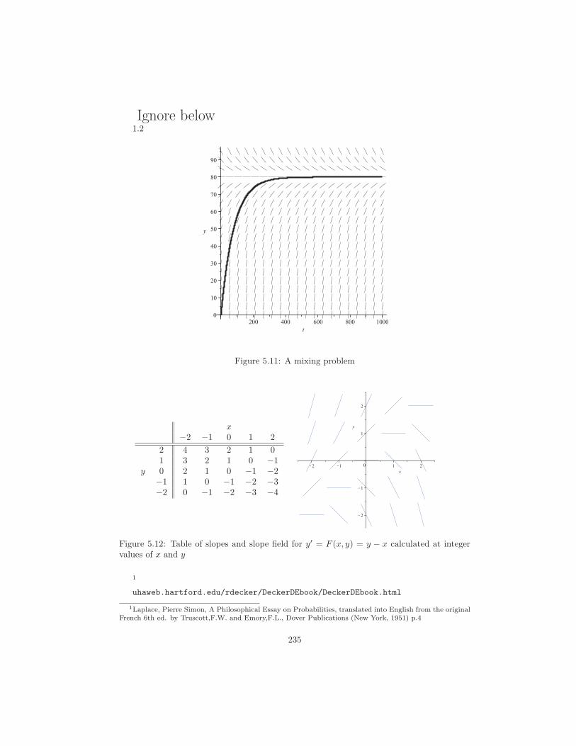
Ignore below1.2
Figure 5.11: A mixing problem
x−2 −1 0 1 2
2 4 3 2 1 01 3 2 1 0 −1
y 0 2 1 0 −1 −2−1 1 0 −1 −2 −3−2 0 −1 −2 −3 −4
Figure 5.12: Table of slopes and slope field for y′ = F (x, y) = y − x calculated at integervalues of x and y
1
uhaweb.hartford.edu/rdecker/DeckerDEbook/DeckerDEbook.html
1Laplace, Pierre Simon, A Philosophical Essay on Probabilities, translated into English from the originalFrench 6th ed. by Truscott,F.W. and Emory,F.L., Dover Publications (New York, 1951) p.4
235
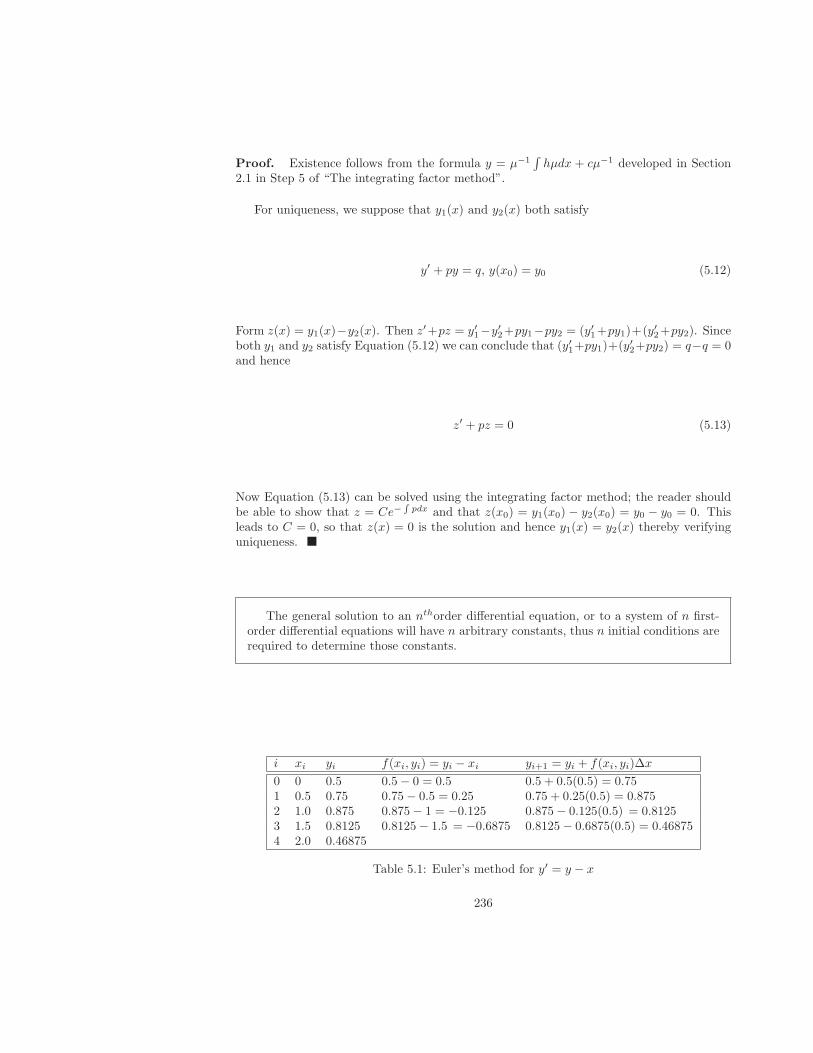
Proof. Existence follows from the formula y = µ−1∫hµdx + cµ−1 developed in Section
2.1 in Step 5 of “The integrating factor method”.
For uniqueness, we suppose that y1(x) and y2(x) both satisfy
y′ + py = q, y(x0) = y0 (5.12)
Form z(x) = y1(x)−y2(x). Then z′+pz = y′1−y′2+py1−py2 = (y′1+py1)+(y′2+py2). Sinceboth y1 and y2 satisfy Equation (5.12) we can conclude that (y′1+py1)+(y′2+py2) = q−q = 0and hence
z′ + pz = 0 (5.13)
Now Equation (5.13) can be solved using the integrating factor method; the reader shouldbe able to show that z = Ce−
∫pdx and that z(x0) = y1(x0) − y2(x0) = y0 − y0 = 0. This
leads to C = 0, so that z(x) = 0 is the solution and hence y1(x) = y2(x) thereby verifyinguniqueness.
The general solution to an nthorder differential equation, or to a system of n first-order differential equations will have n arbitrary constants, thus n initial conditions arerequired to determine those constants.
i xi yi f(xi, yi) = yi − xi yi+1 = yi + f(xi, yi)∆x
0 0 0.5 0.5− 0 = 0.5 0.5 + 0.5(0.5) = 0.751 0.5 0.75 0.75− 0.5 = 0.25 0.75 + 0.25(0.5) = 0.8752 1.0 0.875 0.875− 1 = −0.125 0.875− 0.125(0.5) = 0.81253 1.5 0.8125 0.8125− 1.5 = −0.6875 0.8125− 0.6875(0.5) = 0.468754 2.0 0.46875
Table 5.1: Euler’s method for y′ = y − x
236
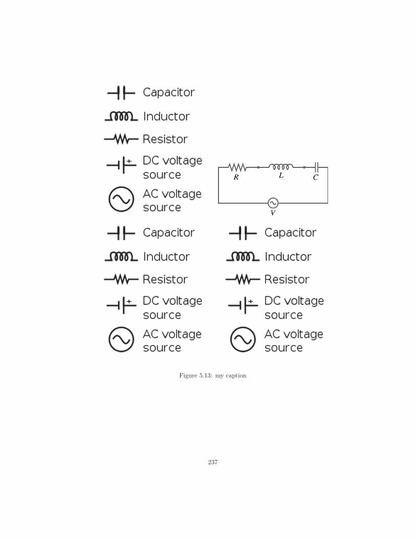
Figure 5.13: my caption
237
Figure 5.14: my caption
238
(a) K = 5 (b) K = 20
(c) K = 100 (d) K = 100, magnified
(e) K = 200 (f) K = 200, magnified
Figure 5.15: Bifurcation diagrams for various K.
239
There are many questions that we can ask about solutions to differential equationsor to initial value problems. Some involve qualitative properties of solutions (whether asolution curve is increasing or decreasing), some quantitative (the value of the dependentvariable at a given value of the independent variable), some short term (small values of theindependent variable) and some long term (large values of the independent variable). Thevarious approaches we have for getting information from a DE or IVP (explicit solutions,graphical methods and numerical methods) are appropriate for some types of questions, andnot for others. Matching an appropriate solution method with a given problem is one of theskills we try to develop in this text.
240