Embed Size (px)
Citation preview

DD2476 Search Engines and Information Retrieval Systems
Lecture 5: Scoring, Weighting, Vector Space Model Hedvig Kjellström [email protected] https://www.kth.se/social/course/DD2476/

Last lecture: IR beyond one shot
Precision-Recall Curve Relevance Feedback Really designed to come after this lecture, but has been moved before this lecture for scheduling reasons Remember these two concepts and do the suggested reading for this lecture (5) before the suggested reading for last lecture (4)

Assignment 1
Thus far, Boolean queries:
BRUTUS AND CAESAR AND NOT CALPURNIA Good for: • Expert users with precise understanding of their
needs and the collection • Computer applications
Not good for: • The majority of users
3
Ch. 6

Problem with Boolean Search: Feast or Famine
Experienced maybe in Task 1.5?
Boolean queries often result in either too few (=0) or too many (1000s) results. • Query 1: “standard user dlink 650”: 200,000 hits • Query 2: “standard user dlink 650 no card found”:
0 hits
It takes a lot of skill to come up with a query that produces a manageable number of hits. • AND gives too few; OR gives too many
4
Ch. 6

Ranked Retrieval
5

Feast or Famine: Not a Problem in Ranked Retrieval
Large result sets no issue • Show top K ( ≈ 10) results • Option to see more results
Premise: the ranking algorithm works well enough
6
Ch. 6

Today
Tf-idf and the vector space model (Manning Chapter 6) • Term frequency, collection statistics • Vector space scoring and ranking
Efficient scoring and ranking (Manning Chapter 7) • Speeding up vector space scoring and ranking
7

Tf-idf and the Vector Space Model (Manning Chapter 6)

Scoring as the Basis of Ranked Retrieval
Wish to return in order the documents most likely to be useful to the searcher
Rank-order documents with respect to a query
Assign a score – say in [0, 1] – to each document • Measures how well document and query “match”
9
Ch. 6

Query-Document Matching Scores
One-term query:
BRUTUS
Term not in document: score 0 More appearances of term in document: higher score
10
Ch. 6

Recall (Lecture 1): Binary Term-Document Incidence Matrix
Document represented by binary vector ∈ {0,1}|V|
11
Sec. 6.2
Antony
and Cleopatra
Julius Caesar
The Tempest Hamlet Othello Macbeth
ANTONY 1 1 0 0 0 0
BRUTUS 1 1 0 1 0 0
CAESAR 1 1 0 1 1 1
CALPURNIA 0 1 0 0 0 0
CLEOPATRA 1 0 0 0 0 0
MERCY 1 0 1 1 1 1
WORSER 1 0 1 1 1 0
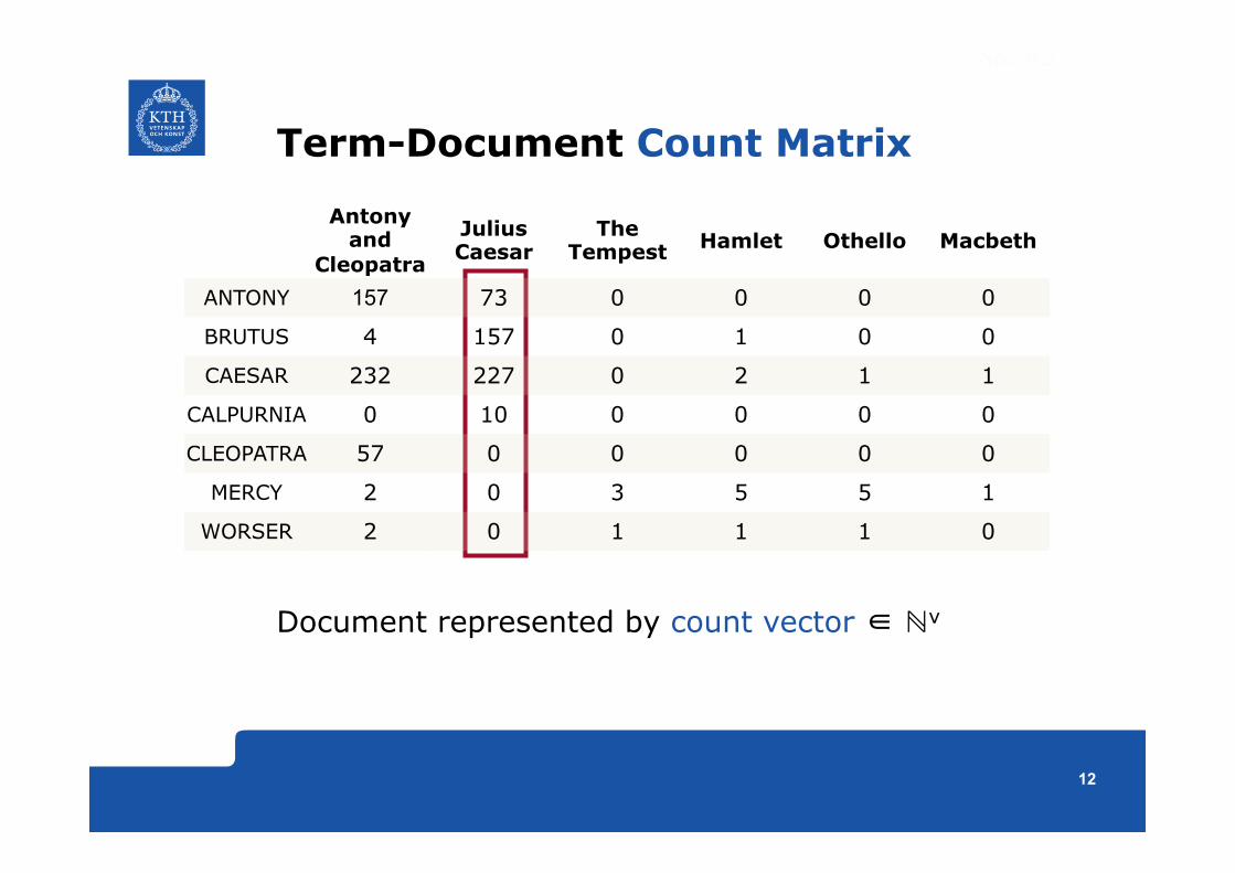
Term-Document Count Matrix
Document represented by count vector ∈ ℕv
12
Sec. 6.2
Antony
and Cleopatra
Julius Caesar
The Tempest Hamlet Othello Macbeth
ANTONY 157 73 0 0 0 0
BRUTUS 4 157 0 1 0 0
CAESAR 232 227 0 2 1 1
CALPURNIA 0 10 0 0 0 0
CLEOPATRA 57 0 0 0 0 0
MERCY 2 0 3 5 5 1
WORSER 2 0 1 1 1 0

Bag of Words Model
Ordering of words in document not considered: • “John is quicker than Mary” ≅ “Mary is quicker than
John”
This is called the bag of words model In a sense, step back: The positional index (Task 1.3) was able to distinguish these two documents Assignment 2 Ranked Retrieval: Back to Bag-of-Words
13

Term Frequency tf
Term frequency tft,d of term t in document d ≅ number of times that t occurs in d
14
frequency = count in IR Antony and
Cleopatra
ANTONY 157

Log-Frequency Weighting
Raw term frequency is a bit overestimated: • A document with 10 occurrences of the term is
more relevant than a document with 1 occurrence of the term
• But arguably not 10 times more relevant Alternative is log-frequency weight of term t in document d
15
Sec. 6.2
⎩⎨⎧ >+
=otherwise 0,
0 tfif, tflog 1 10 t,dt,d
t,dw

Simple Query-Document Score
Queries with >1 terms
Score for a document-query pair: sum over terms t in both q and d:
score The score is 0 if none of the query terms is present in the document What is the problem with this measure?
16
Sec. 6.2
=X
t2q\d
tft,d

Document Frequency
Rare terms are more informative than frequent terms Example: rare word ARACHNOCENTRIC • Document containing this term is very likely to be
relevant to query ARACHNOCENTRIC → High weight for rare terms like ARACHNOCENTRIC
Example: common word THE • Document containing this term can be about anything
→ Very low weight for common terms like THE
We will use document frequency (df) to capture this.
17
Sec. 6.2.1

idf Weight
dft is the document frequency of term t: the number of documents that contain t • dft is an inverse measure of the informativeness of t • dft ≤ N
Informativeness idf (inverse document frequency) of t: • log (N/dft) instead of N/dft to “dampen” the effect
– Mathematical reasons in lecture 7!
18
)/df( log idf 10 tt N=
Sec. 6.2.1

Exercise 2 Minutes
Suppose N = 1,000,000 Fill in the idft column
19
term dft idft
calpurnia 1
animal 100
sunday 1,000
fly 10,000
under 100,000
the 1,000,000
)/df( log idf 10 tt N=

Effect of idf on Ranking
Does idf have an effect on ranking for one-term queries, like IPHONE?
Only effect for >1 term • Query CAPRICIOUS PERSON: idf puts more weight
on CAPRICIOUS than PERSON.
20

Collection vs. Document Frequency
Collection frequency of t: total number of occurrences of t in the collection, counting multiple occurrences
Example:
Which word is a better search term (and should get a higher weight)?
21
Word Collection frequency Document frequency
insurance 10440 3997
try 10422 8760
Sec. 6.2.1

tf-idf Weighting
tf-idf weight of a term: product of tf weight and idf weight Best known weighting scheme in information retrieval • Note: the “-” in tf-idf is a hyphen, not a minus
sign! • Alternative names: tf.idf, tf x idf
Increases with the number of occurrences within a document Increases with the rarity of the term in the collection
22
Sec. 6.2.2
wt,d = tft,d ⇥ log10(N/dft)
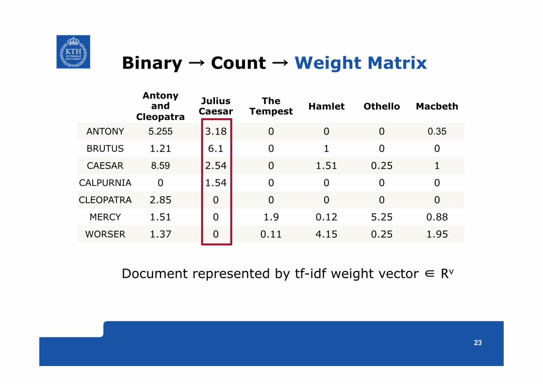
Binary → Count → Weight Matrix
Document represented by tf-idf weight vector ∈ Rv
23
Sec. 6.3
Antony
and Cleopatra
Julius Caesar
The Tempest Hamlet Othello Macbeth
ANTONY 5.255 3.18 0 0 0 0.35
BRUTUS 1.21 6.1 0 1 0 0
CAESAR 8.59 2.54 0 1.51 0.25 1
CALPURNIA 0 1.54 0 0 0 0
CLEOPATRA 2.85 0 0 0 0 0
MERCY 1.51 0 1.9 0.12 5.25 0.88
WORSER 1.37 0 0.11 4.15 0.25 1.95

Documents as Vectors
So we have a |V|-dimensional vector space • Terms are axes/dimensions • Documents are points in this space
Very high-dimensional • Order of 107 dimensions when for a web search
engine
Very sparse vectors - most entries zero
24
Sec. 6.3

Queries as Vectors
Key idea 1: Represent queries as vectors in same space
Key idea 2: Rank documents according to proximity to query in this space • proximity = similarity of vectors • proximity ≈ inverse of distance
Recall: • Get away from Boolean model • Rank more relevant documents higher than less
relevant documents
25
Sec. 6.3

Formalizing Vector Space Proximity
First cut: Euclidean distance? Euclidean distance is a bad idea . . . . . . because Euclidean distance is large for vectors of different lengths • What determines
length here?
26
Sec. 6.3
€
q − dn 2

Exercise 5 Minutes
Euclidean distance bad for • vectors of different length
(documents with different #words)
• high-dimensional vectors (large dictionaries)
Discuss in pairs: • Can you come up with a better difference
measure?
27

Use Angle Instead of Distance
Thought experiment: take a document d and append it to itself. Call this document d′ “Semantically” d and d′ have the same content The Euclidean distance between the two documents can be quite large The angle between the two documents is 0, corresponding to maximal similarity Key idea: • Length unimportant • Rank documents according to angle from query
28
Sec. 6.3

Problems with Angle
Angles expensive to compute – arctan
Find a computationally cheaper, equivalent measure • Give same ranking order ≅ monotonically
increasing/decreasing with angle
Any ideas?
29
Sec. 6.3

Cosine More Efficient Than Angle
30
Sec. 6.3
Monotonically decreasing
0 10 20 30 40 50 60 70 80 900
0.1
0.2
0.3
0.4
0.5
0.6
0.7
0.8
0.9
1
angle
cos(angle)

Length Normalization
Computing cosine similarity involves length-normalizing document and query vectors L2 norm:
Dividing a vector by its L2 norm makes it a unit (length) vector (on surface of unit hypersphere) Recall: • Length unimportant • Rank documents according to angle from query
31
∑=i ixx 2
2
!
Sec. 6.3

Cosine Similarity
qi is the tf-idf weight of term i in the query di is the tf-idf weight of term i in the document
is the cosine similarity of q and d = the cosine of the angle between q and d.
32
€
cos( q , d )
€
cos( q , d ) =
q q 2
•
d d
2
= q • d
q 2 d
2
=qidii=1
V∑
qi2
i=1
V∑ di
2
i=1
V∑
dot / scalar / inner product

Cosine Similarity
In reality: • Length-normalize when
document added to index:
• Length-normalize query:
• Fast to compute cosine similarity:
33
€
cos( q , d ) = q • d = qidii=1
V∑
€
d ←
d d
2
€
q ← q q 2

Cosine Similarity Example
How similar are the novels • SaS: Sense and Sensibility • PaP: Pride and Prejudice • WH: Wuthering Heights?
Term frequency tft
34
term SaS PaP WH
affection 115 58 20
jealous 10 7 11
gossip 2 0 6
wuthering 0 0 38
No idf weighting!

Cosine Similarity Example
Log frequency weights
35
⎩⎨⎧ >+
=otherwise 0,
0 tfif, tflog 1 10 t,dt,d
t,dw
term SaS PaP WH affection 3.06 2.76 2.30 jealous 2.00 1.85 2.04 gossip 1.30 0 1.78 wuthering 0 0 2.58

Cosine Similarity Example
After length normalization , cos(SaS,PaP) ≈ 0.789*0.832 + 0.515*0.555 + 0.335*0 + 0*0 ≈ 0.94 cos(SaS,WH) ≈ 0.79 cos(PaP,WH) ≈ 0.69 Why is cos(SaS,PaP) > cos(*,WH)? 36
term SaS PaP WH affection 0.789 0.832 0.524 jealous 0.515 0.555 0.465 gossip 0.335 0 0.405 wuthering 0 0 0.588
€
d ←
d d
2
€
d = w1,d ,…,w4,d[ ]

Computing Cosine Scores
37
Sec. 6.3
Summary – vector space ranking
Represent the query as a tf-idf vector
Represent each document as a tf-idf vector
Compute the cosine similarity score for the query vector and each document vector
Rank documents with respect to the query by score
Return the top K (e.g., K = 10) to the user
38

Efficient Scoring and Ranking (Manning Chapter 7)

Efficient Cosine Ranking
Find the K docs in the collection “nearest” to the query ⇒ K largest query-document cosine scores
Up to now: Linear scan through collection • Did not make use of sparsity in term space • Computed all cosine scores
Efficient cosine ranking: • Computing each cosine score efficiently • Choosing the K largest scores efficiently
40
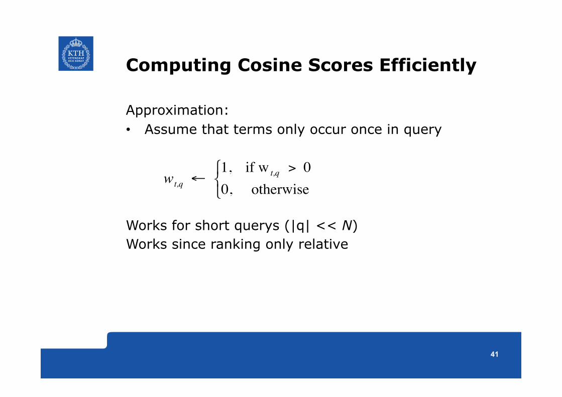
Computing Cosine Scores Efficiently
Approximation: • Assume that terms only occur once in query
Works for short querys (|q| << N) Works since ranking only relative
41
€
wt,q ← 1, if w t,q > 00, otherwise# $ %

Computing Cosine Scores Efficiently
42
Sec. 7.1
Speedup here

Computing Cosine Scores Efficiently
Downside of approximation: sometimes get it wrong • A document not in the top K may creep into the list
of K output documents
How bad is this?
Cosine similarity is only a proxy (Task 1.5) • User has a task and a query formulation • Cosine matches documents to query • Thus cosine is anyway a proxy for user happiness • If we get a list of K documents “close” to the top K
by cosine measure, should be ok
43
Sec. 7.1.1
Choosing K Largest Scores Efficiently
Retrieve top K documents wrt query • Not totally order all documents in collection
Do selection: • avoid visiting all documents
Already do selection: • Sparse term-document incidence matrix, |d| << N • Many cosine scores = 0 • Only visits documents with nonzero cosine scores
(≥1 term in common with query)
44
Sec. 7.1

Choosing K Largest Scores Efficiently Generic Approach
Find a set A of contenders, with K < |A| << N • A does not necessarily contain the top K, but has
many docs from among the top K • Return the top K documents in A
Think of A as pruning non-contenders
Same approach used for any scoring function!
Will look at several schemes following this approach
45
Sec. 7.1.1

Choosing K Largest Scores Efficiently Index Elimination
Basic algorithm FastCosineScore only considers documents containing at least one query term • All documents have ≥1 term in common with
query
Take this further: • Only consider high-idf query terms • Only consider documents containing many query
terms
46
Sec. 7.1.2
Choosing K Largest Scores Efficiently Index Elimination, only high-idf
Example: CATCHER IN THE RYE
Only accumulate scores from CATCHER and RYE Intuition: • IN and THE contribute little to the scores – do not
alter rank-ordering much • Compare to stop words Benefit: • Posting lists of low-idf terms have many
documents → eliminated from set A of contenders
47
Sec. 7.1.2

Choosing K Largest Scores Efficiently Index Elimination, several query terms
Example: CAESAR ANTONY CALPURNIA BRUTUS
Only compute scores for documents containing ≥3 query terms
48
Sec. 7.1.2
Brutus
Caesar
Calpurnia
1 2 3 5 8 13 21 34
2 4 8 16 32 64 128
13 16
Antony 3 4 8 16 32 64 128
32

Choosing K Largest Scores Efficiently Champion Lists
Precompute for each dictionary term t, the r documents of highest tf-idftd weight • Call this the champion list (fancy list, top docs) for t
Benefit: • At query time, only compute scores for documents in
the champion lists – fast Issue: • r chosen at index build time • Too large: slow • Too small: r < K
49
Sec. 7.1.3
Exercise 5 Minutes
Index Elimination: consider only high-idf query terms and only documents with many query terms Champion Lists: for each term t, consider only the r documents with highest tf-idftd values Think quietly and write down: • How do Champion Lists relate to Index
Elimination? Can they be used together? • How can Champion Lists be implemented in an
inverted index?
50
Sec. 7.1.3

Choosing K Largest Scores Efficiently Static Quality Scores
Develop idea of champion lists
We want top-ranking documents to be both relevant and authoritative • Relevance – cosine scores • Authority – query-independent property
Examples of authority signals • Wikipedia pages (qualitative) • Articles in certain newspapers (qualitative) • A scientific paper with many citations (quantitative) • PageRank (quantitative)
51
Sec. 7.1.4
More in Lecture 6

Choosing K Largest Scores Efficiently Static Quality Scores
Assign query-independent quality score g(d) in [0,1] to each document d
net-score(q,d) = g(d) + cos(q,d) • Two “signals” of user happiness • Other combination than equal weighting
Seek top K documents by net score
52
Sec. 7.1.4

Choosing K Largest Scores Efficiently Champion Lists + Static Quality Scores
Can combine champion lists with g(d)-ordering
Maintain for each term t a champion list of the r documents with highest g(d) + tf-idftd
Seek top K results from only the documents in these champion lists
53
Sec. 7.1.4

Next
Assignment 1 left? • You can present it at the session for Assignment 2 • Reserve two slots, one for each assignment!
Lecture 6 (February 23, 13.15-15.00) • B3 • Readings: Manning Chapter 21
Avrachenkov Sections 1-2
Lecture 7 (February 24, 10.15-12.00) • B3 • Readings: Manning Chapters 11, 12
54