DC-motor PID control

This version: November 1, 2017

REGLERTEKNIK

AUTOMATIC CONTROL

LINKÖPING

Name:

P-number:

Date:

Passed:

Chapter 1

Introduction

The purpose of this lab is to give an introduction to PID control. We ex-periment with PID controllers to control the angle and angular velocity ofa small arm attached to a DC-motor (see cover). This simple experimentmimics typical applications in practice, such as the robotic hand in the fig-ure below.

Figure 1.1: Robotic hand using 15 DC-motors to position 5 fingers inde-pendently. High-precision control of joint angles is required forhigh-precision picking of objects, gentle grabbing, forming ges-tures etc.

1

1.1 Hardware set-up

The lab is based on three main hardware components.

To begin with, we have a standard desktop computer. This computer isused to automatically develop and deploy code using MATLAB and SIMULINK

models.

To supply power to the DC-motor and perform measurements of motor an-gles, we use a board with an Arduino micro-controller which runs the auto-generated code. It also communicates with the desktop computer and thusallows us to look at the measurements.

The motor we experiment with is a simple DC-motor with a wheel and anarm attached. The motor is normally part of a LEGO Mindstorms kit.

The Arduino board together with the motor and attachments is called theMinSeg.

1.2 Troubleshooting

The wheels turn slowly and/or erratically Make sure the tires do not rubagainst the motor. You can pull the wheels apart as they slide on the wheelaxis.

Complaints about COM port or connection when downloading to boardDisconnect USB-cable and connect it again. Make sure cable is firmly at-ached on both ends. If it still does not work after several tries, save yourmodel and restart MATLAB.

Complaints about OUT OF MEMORY when compiling code Save your modeland restart MATLAB.

2

Chapter 2

Preparation

The questions below, and all questions throughout the document markedas Preparation must be completed by all students before attending the lab.Note that there are additional preparation exercises in Chapter 3.

Solutions to all questions should be available upon request from the labassistant, and the preparation exercises in Chapter 3 are preferably writtenin this printed documented.

When the lab starts, it is assumed you have done all preparations, and havea clear idea of the tasks that will be performed during the lab.

Note, although there are 15 question below, many of them are variants ofexactly the same question, repeated for different setups.

Finally, note that essentially all computations performed below relate topractical experiments that we will conduct during the lab, i.e., they all havephysical meaning and it is important to see these connections during thelab.

Preparation 1 Read Section 3.1-3.6 in the course book by Ljung & Glad.

Preparation 2 (P-controlled angle) Suppose we use a P-controller to con-trol the angle y(t ) = θ(t ) to follow a reference angle r (t ), i.e., u(t ) = KP(r (t )−y(t )) or equivalently U(s) = KP(R(s)−Y(s)) where KP > 0. The transfer func-tion from requested voltage u(t ) to angle y(t ) is given by G(s) = 1.35

s(0.1s+1) .Show that the closed-loop system from reference to angle is given by

3

Y(s) = 1.35KP

0.1s2 + s +1.35KPR(s) (2.1)

Preparation 3 (P-controlled angle) Suppose the motor is at the angle y(t ) =0 and we change the reference from 0 to r (t ) = π/2. Assuming we are usingthe gain KP = 3, which input voltage u(t ) will initially be requested by thecontroller when the step is performed?

Preparation 4 (P-controlled angle) Write the closed-loop transfer function

in the standard form G(s) = ω20

s2+2ζω0s+ω20

(i.e., identify the parameters ζ and

ω0 as functions of KP) and explain based on this how speed and oscillatorybehavior of the closed-loop system is related to KP. Suitable theory can befound on page 37 in the course book.

Preparation 5 (P-controlled angle) For simple systems, overshoot and os-cillations can be predicted to occur when poles become complex, and thelarger the complex part is compared to the real part, the larger the over-shoot and oscillations are. Show that the closed-loop poles are complex whenKP > 25

13.5 .

Preparation 6 (P-controlled angle) Assume a disturbance v(t ) is acting onthe input to the system, i.e., the actual input to the system is given by u(t )+v(t ) where v(t ) is unknown, see Figure 2.1.

Figure 2.1: Disturbance acting on the input.

With U(s) = F(s)(R(s)−Y(s)), show that control error e(t ) = r (t )−y(t ) is givenby

E(s) = 1

1+F(s)G(s)R(s)− G(s)

1+F(s)G(s)V(s) (2.2)

4

Preparation 7 (P-controlled angle) With G(s) = 1.35s(0.1s+1) and the P-controller

F(s) = KP, show that the error signal in the previous exercise evaluates to

E(s) = 0.1s2 + s

0.1s2 + s +1.35KPR(s)− 1.35

0.1s2 + s +1.35KPV(s) (2.3)

Preparation 8 (P-controlled angle) Let the reference be a step with ampli-tude A (R(s) = A

s ) and the input disturbance be a step with (unknown) am-

plitude B (V(s) = Bs ) (i.e., we are modeling constant signals). Use the final

value theorem to show that the steady-state value of the error, limt→∞ e(t ),converges to −B

KPwhen a P-controller F(s) = KP is used. Hence, as long as there

is no input disturbance, we can track a constant reference angle without anysteady-state error using a simple P-controller, but an input disturbance willcause a steady-state error. By increasing KP this error can be decreased.

Preparation 9 (PI-controlled angle) Now use a PI-controller F(s) = KP+KIs =

KP s+KIs . Use the same setup as above with constant reference and disturbance,

and show that the steady-state error converges to 0. In other words, integralaction ( 1

s , pole in the origin) in the controller can help us to counteract aconstant input disturbance.

Preparation 10 (PD-controlled angle) Now use a PD-controller to controlthe angle y(t ), i.e., F(s) = (KP +KDs). Show that the closed-loop system fromR(s) to Y(s) is given by (we skip the input disturbance now)

Y(s) = 1.35(KP +KDs)

0.1s2 + (1.35KD +1)s +1.35KPR(s) (2.4)

Preparation 11 (PD-controlled angle) Show that all closed-loop poles are

real if KD ≥p

54KP−1013.5 , i.e., the larger KP we use, the larger KD we need to keep

all poles real.

Preparation 12 (P-controlled angular velocity) Now consider control of an-gular velocity, y(t ) =ω(t ) = θ(t ). The transfer function from requested volt-age u(t ) to angular velocity y(t ) is given by G(s) = 1.35

(0.1s+1) (i.e., the only dif-ference compared to the angle model is the removed integrator). Show thatthe closed-loop system from reference to angular velocity when a P-controllerF(s) = KP is used is given by

Y(s) = 1.35KP

0.1s +1+1.35KPR(s) (2.5)

5

Preparation 13 (P-controlled angular velocity) Show that the time-constantof the closed-loop system is 1

10+13.5KP, i.e., increasing KP decreases the time-

constant and makes the closed-loop system faster.

Preparation 14 (P-controlled angular velocity) Show that the error signalwith a reference and an input disturbance is given by

E(s) = 0.1s +1

0.1s +1+1.35KPR(s)− 1.35

0.1s +1+1.35KPV(s) (2.6)

Preparation 15 (P-controlled angular velocity) Let R(s) = As and V(s) = B

s ,and use the final value theorem to show that the steady-state value of theerror converges to A

1+1.35KP− 1.35B

1+1.35KPwhen a P-controller F(s) = KP is used.

In other words, constant non-zero angular velocity references cannot be fol-lowed without a steady-state error using a P-controller, even in the perfectcase when there are no input disturbances.

Preparation 16 (PI-controlled angular velocity) Use a PI-controller F(s) =KP+KI

s . Use the same setup as above with a reference signal and input distur-bance, and show that the steady-state error converges to 0. In other words,integral action in the controller allows us to track a constant reference signalwithout steady-state error, and eliminates steady-state errors due to constantinput disturbances.

Preparation 17 (Summary of steady-state errors) We considered a systemwith an integrator (pole in the origin) when we analyzed angle control, and asystem without an integral in the angular velocity control case. We have alsostudied controllers without integrator (P, PD), and controllers with integra-tor (PI). In the table on the next page, mark the cases where theory predictsthat we can track a constant reference perfectly, and eliminate a constantinput disturbances. Since external signals (references, disturbances) act in-dependently, you should consider the results independently, i.e. when youstudy reference tracking, simply assume input disturbance is 0, and whenyou consider input disturbances, you assume the reference is zero.

Preparation 18 Read the complete lab-pm. There are some theoretical ques-tions in the pm which you are supposed to complete as preparation.

Preparation 19 Print this document. You must bring a physical copy to thelab.

6

F(s) (no integral) F(s) (has integral)G(s)

(no integral)ä Reference tracked perfectly

ä Input disturbance eliminatedä Reference tracked perfectlyä Input disturbance eliminated

G(s)(has integral)

ä Reference tracked perfectlyä Input disturbance eliminated

ä Reference tracked perfectlyä Input disturbance eliminated

7

Chapter 3

The lab

Items labeled Preparation are questions you are supposed to solve and fillout before attending the lab.

Items labeled Task are questions you solve when attending the lab and haveaccess to the hardware.

In the lab, we will address two different scenarios ; control of angle, andcontrol of angular velocity, and we will use various PID variants.

• P-control of angle

• PD-control of angle

• PID-control of angle

• P-control of angular velocity

• PI-control of angular velocity

The goal of the lab is to understand how the different parts of the PID con-troller influence closed-loop behavior and performance.

The design of the controllers will be completely model free (i.e., they aretuned by simply changing the gains without any computations). However,almost all phenomena seen (speed, steady-state errors, and oscillations)can be explained by the analysis you have done in the preparation exerciseswhere a model of the DC-motor is used. Hence, it is important that youconnect the dots between experimental results, and the predictions andanalysis made in the preparation exercises.

8

3.1 DC-motor model

In the first lab, we derived and worked with a model describing the angularvelocity ω(t ) = θ(t ) of the motor, when a voltage uA(t ) was applied on themotor. Experiments typically found that 0.1ω(t )+ω(t ) = 1.9uA(t ) whichcorresponds to the transfer function 1.9

0.1s+1 (look in your notes from the firstlab!). In this lab, we will reuse this model, with some minor changes.

Figure 3.1: Our models now includes the motor driver (black chip) and de-scribes the angle of the motor y(t ) = θ(t ) or angular velocityy(t ) = ω(t ) = θ(t ), when sending voltage requests u(t ) to themotor driver.

To begin with, our input u(t ) will not be the voltage applied to the motor(uA(t ), which we measured using a multimeter), but the voltage sent to mo-tor driver chip. The reason is that the voltage sent to the motor driver is theonly signal we can manipulate directly and thus use for control. When 4.5Vis sent to the motor driver chip by the Arduino micro-controller, the result-ing voltage on the motor is 3.2V. Hence, a reasonable model for the motordriver (black chip) is a simple gain uA(t ) = (3.2/4.5)u(t ).

Our initial focus will be the angle of the motor (y(t ) = θ(t )). Going from amodel of the angular velocityω(t ) to angle is done by integrating the veloc-ity y(t ) = ∫

ω(τ)dτ

Preparation 20 Show that a model for the angle y(t ) = θ(t ) given the inputu(t ) is given by

Y(s) = G(s)U(s) = 1.35

s(0.1s +1)U(s) (3.1)

9

Note that this is the model you have used in the preparation exercises, i.e.,your theoretical predictions have been derived using a slight extension ofthe model you developed in the first lab.

3.2 Control of angle

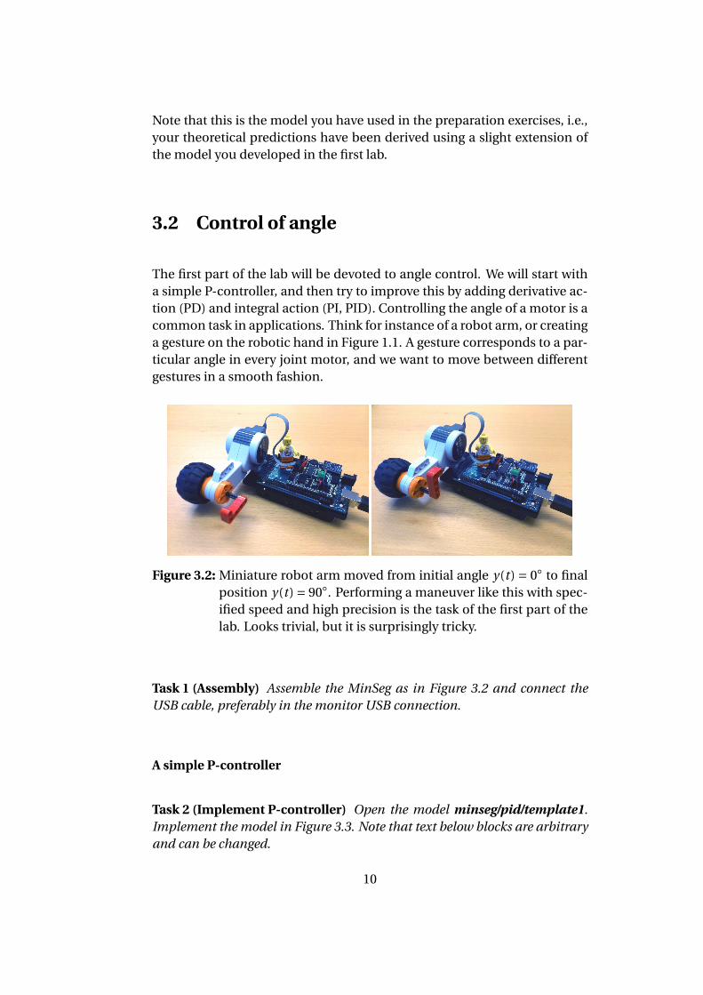
The first part of the lab will be devoted to angle control. We will start witha simple P-controller, and then try to improve this by adding derivative ac-tion (PD) and integral action (PI, PID). Controlling the angle of a motor is acommon task in applications. Think for instance of a robot arm, or creatinga gesture on the robotic hand in Figure 1.1. A gesture corresponds to a par-ticular angle in every joint motor, and we want to move between differentgestures in a smooth fashion.

Figure 3.2: Miniature robot arm moved from initial angle y(t ) = 0◦ to finalposition y(t ) = 90◦. Performing a maneuver like this with spec-ified speed and high precision is the task of the first part of thelab. Looks trivial, but it is surprisingly tricky.

Task 1 (Assembly) Assemble the MinSeg as in Figure 3.2 and connect theUSB cable, preferably in the monitor USB connection.

A simple P-controller

Task 2 (Implement P-controller) Open the model minseg/pid/template1.Implement the model in Figure 3.3. Note that text below blocks are arbitraryand can be changed.

10

• Sum: can be found in Commonly used blocks. Make sure you under-stand why there is a + and a − in the computation.

• Slider gain: This implements the controller gain KP. It is found underMath operations.

• Pulse generator: This is the reference signal. It is found under Sources.Set the amplitude to π/2, period to 10 and pulse width 50% (i.e., createa reference signal r (t ) which switches between 0 and π/2 every 5 sec-onds). Note that the amplitude π/2 corresponds to the constant A inthe preparation exercises.

• Plot scope: Found under Sinks (or copy the one in model).

Remember to save the file after implementing the model!

Figure 3.3: P-control of angle θ(t ).

Task 3 (Experiment with proportional gain) Download the controller to theArduino with the green run button. What happens with the speed of thestep-response when you increase KP? (make sure you are looking at the cor-rect plot, i.e., the plot of reference angle r (t ) and measured angle y(t )) Youwill have to increase the max value in the Slider gain as you investigate step-responses for increasingly larger KP (try for instance 1,2,4,6,8,10 to really seethe effects). Is the result consistent with Preparation 4?

11

Task 4 (Overshoots and complex poles) Find the value on KP for which youclearly start seeing overshoots in the step response (value of y(t ) at some timelarger than the value it finally converges to, or smaller when steps in theother direction are performed). How does this value compare to the theo-retical prediction on complex poles (and thus possibly oscillatory response)for the closed-loop system in Preparation 5?

Task 5 (Steady-state errors) Let us study how the steady-state error changeswhen you alter KP. How large are the steady-state errors for, e.g., KP = 1,5and 10? Based on the observation coupled with results in Preparation 8, isit likely that there is no input disturbances?

Task 6 (Tuning speed and steady-state behaviour) Is it possible to tune thecontroller to achieve a very slow smooth movement while having a smallsteady-state error? Combine the theoretical predictions from Preparation 4and Preparation8 and confirm in practice.

12

Task 7 (Excessively large gain) By increasing the gain, you see that the steady-state error becomes smaller, as theory predicts. However, what happens if youmake KP really large (say, 40)?

Task 8 (Failure of theory) From Preparation 4 and page 37 in the coursebook we draw the conclusion that the closed-loop poles distance to the originis proportional to

pKP. Hence, theory tells us the step-response should be

significantly faster if we change KP from 20 to 40. In practice this is not thecase (check!, look for instance on the time it takes to go from 0 until it crossesthe reference the first time). Can you figure out why it doesn’t get any faster?Hint: Look at the plot of the requested control input u(t ) during the stepsand note that the largest possible voltage available through an USB cable is4.5V.

Task 9 (Summary on proportional feedback) Summarize the main effectKP has on speed, steady-state error and overshoots & oscillations.

13

Derivative action to reduce oscillations

When increasing KP, overshoots and oscillations become problematic. Tocounteract this, we will add derivative action to the controller, i.e., let thecontrol signal depend on how fast the error changes. If the error is deceas-ing rapidly (e(t ) very negative), we should use less input voltage and per-haps even brake and apply voltage in the negative direction to avoid anovershoot. As we have seen in the preparation exercises, by using a suffi-ciently large KD, complex poles can be avoided completely, thus reducingthe likelihood of overshoots and oscillations.

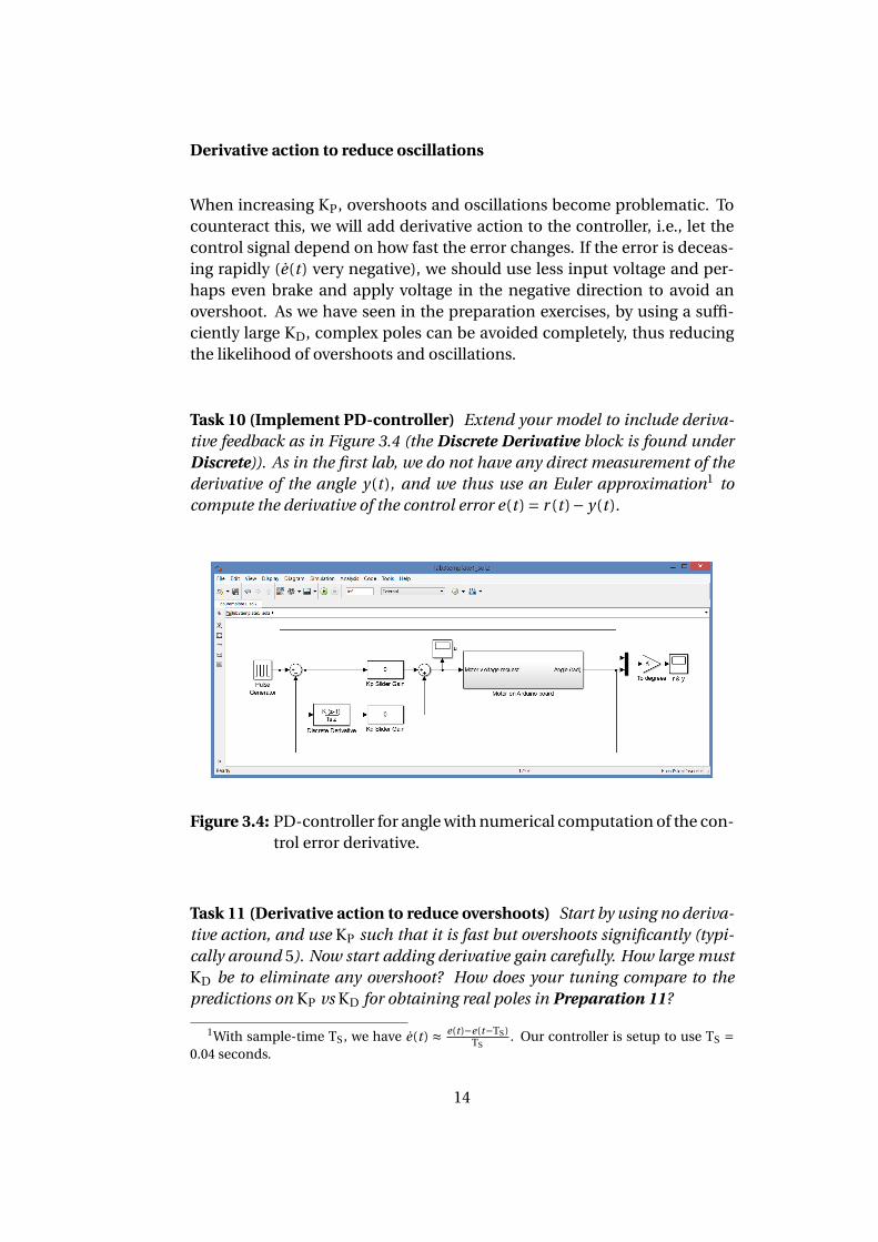
Task 10 (Implement PD-controller) Extend your model to include deriva-tive feedback as in Figure 3.4 (the Discrete Derivative block is found underDiscrete)). As in the first lab, we do not have any direct measurement of thederivative of the angle y(t ), and we thus use an Euler approximation1 tocompute the derivative of the control error e(t ) = r (t )− y(t ).

Figure 3.4: PD-controller for angle with numerical computation of the con-trol error derivative.

Task 11 (Derivative action to reduce overshoots) Start by using no deriva-tive action, and use KP such that it is fast but overshoots significantly (typi-cally around 5). Now start adding derivative gain carefully. How large mustKD be to eliminate any overshoot? How does your tuning compare to thepredictions on KP vs KD for obtaining real poles in Preparation 11?

1With sample-time TS , we have e(t ) ≈ e(t )−e(t−TS )TS

. Our controller is setup to use TS =0.04 seconds.

14

Task 12 (Excessively large derivative gain) What happens if you use a re-ally large value on KD? What could the reason be? Hint: we cannot measurethe derivative θ(t ) but estimate it from noisy measurements of θ(t ).

Task 13 Try to make the system as fast as possible, with no movements re-maining after 1 second and less than 5◦ overshoot (i.e., implement a con-troller you would be proud to sell!). Remember to look at the actual move-ments and not just the plots. Which tuning do you arrive at?

Where does the steady-state error come from?

Based on the preparation exercises, we know that there should be no steady-state error, unless there is an input disturbance (or our models and as-sumptions are completely wrong!). There is no direct input disturbanceacting on the system as far as we know, but there is an unmodeled effectthat can be interpreted as a disturbance. The motor driver chip (see Fig-ure 3.1) has an electrical dead-zone which causes it to output 0V for any

15

requested voltage |u(t )| ≤ 0.7V (the exact size on the dead-zone varies be-tween different individual chips), see Figure 3.5 for an illustration. By see-ing the difference between the applied voltage with dead-zone (solid line)and our model 3.2

4.5 u(t ) (dashed line) as an input disturbance, we can try tocompensate for it using integral action in the controller. According to thetheoretical result in Preparation 9, this might eliminate the problem.

Figure 3.5: The motor driver chip has a dead-zone. When the requestedvoltage |u(t )| is small (here |u(t )| ≤ 0.7V), no voltage is ap-plied on the motor. The difference between the actual voltage(solid line) and our linear approximation 3.2

4.5 u(t ) (dashed) canbe thought of as an input disturbance v(t ). It is not constant asit depends on u(t ), but thinking of the effect of the dead-zoneas an input disturbance is a good start.

Intuitively, what happens with a P-controller is that when the error e(t ) issmall enough, the input KPe(t ) will become so small that it is clipped in thedead-zone, effectively turning of the DC-motor, and it will slow down dueto friction etc and stop at some point where typically e(t ) 6= 0. By increasingKP, the region where it is turned off will become smaller, but there will stillbe some region where the dead-zone causes it to be turned off.

16

Integral action to (try to) eliminate steady-state error

We will now try (and most likely fail!) to eliminate the steady-state error us-ing integral action. In theory according to Preparation 9, if the input dis-turbance is constant, a PI controller should be able to eliminate any steady-state error.

Task 14 (Implement PID-controller) Extend your SIMULINK model to in-clude integral action as in Figure 3.6.

• The Discrete-time integrator2 block is found under Discrete

• In the Discrete-time integrator block, set the sample time to −1 (thismeans it uses our sample-time TS = 0.04s).

• Change the period time in the pulse generator to 30 seconds (this willallow us to study the steady-state error for longer times before it switchesreference value).

Note that we have switched the location of the gain and the integral. Withthis order, the integral output will stay constant if KI = 0. If we keep inte-grating while KI is zero, and then change KI to a non-zero value, the integralmight have a huge value, leading to huge inputs.

Task 15 (Integral action and oscillations) Start with, e.g., KP = 2,KI = 5 andKD = 0. Try reducing and increasing KI. What happens and what does thistell us about how KI influence pole locations in the closed-loop system? Tryadding derivative action KD to see if oscillations introduced by the integralpart can be reduced.

2The integral is approximated using a rectangular approximation∫ t

0 e(τ)dτ ≈ TSe(0)+TSe(TS)+TSe(2Ts )+ . . .+Ts e(t )

17

Figure 3.6: PID controller for angle control. Note that the order of gain andintegral has been switched. By performing the computations inthis order we ensure the integral stops integrating if we turn offthe integral action with KI = 0.

Task 16 (Steady-state error) Can the steady-state error be eliminated usingKI? While running, look at the plot of the integral term added to the controlinput, and see how it keeps increasing and decreasing when the steady-stateerror is constant and non-zero. The integrator tries to find the value neededto compensate for the dead-zone, but cannot find any such suitable constantvalue (as it depends on the changing input).

Although integral action probably fails to solve the problem completelyhere (due to the complicated dead-zone behavior, the input disturbance isnot constant), it will be a very useful tool later when we control the angularvelocity. Always try integral action when you have steady-state errors. Ifthis does not work, you might have to use more tailor-made and advancedsolutions, as we will do now.

18

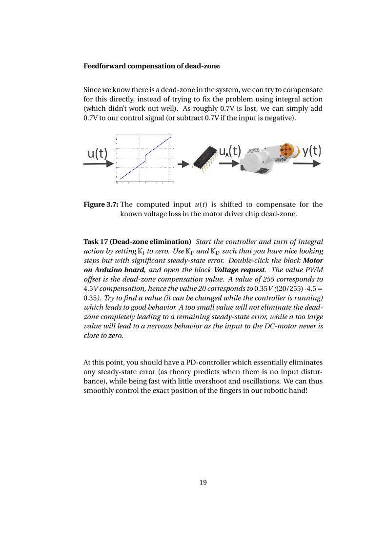
Feedforward compensation of dead-zone

Since we know there is a dead-zone in the system, we can try to compensatefor this directly, instead of trying to fix the problem using integral action(which didn’t work out well). As roughly 0.7V is lost, we can simply add0.7V to our control signal (or subtract 0.7V if the input is negative).

Figure 3.7: The computed input u(t ) is shifted to compensate for theknown voltage loss in the motor driver chip dead-zone.

Task 17 (Dead-zone elimination) Start the controller and turn of integralaction by setting KI to zero. Use KP and KD such that you have nice lookingsteps but with significant steady-state error. Double-click the block Motoron Arduino board, and open the block Voltage request. The value PWMoffset is the dead-zone compensation value. A value of 255 corresponds to4.5V compensation, hence the value 20 corresponds to 0.35V ((20/255) ·4.5 =0.35). Try to find a value (it can be changed while the controller is running)which leads to good behavior. A too small value will not eliminate the dead-zone completely leading to a remaining steady-state error, while a too largevalue will lead to a nervous behavior as the input to the DC-motor never isclose to zero.

At this point, you should have a PD-controller which essentially eliminatesany steady-state error (as theory predicts when there is no input distur-bance), while being fast with little overshoot and oscillations. We can thussmoothly control the exact position of the fingers in our robotic hand!

19

3.3 Control of angular velocity

Our task now is to have the motor rotate at a specified angular velocity. Atypical application would be a cruise-controller in a car (to obtain a desiredspeed, the wheels must rotate with a particular angular velocity) or a robotarm which is programmed to move at a particular speed when performinga task such as welding or painting.

Task 18 (Implement PI-controller) Open the model template2 and imple-ment a PI-controller of the angular velocity as illustrated in Figure 3.8. Notethat the output from the Arduino board block is the angular velocity now(computed by Euler approximations from angle measurements)

• Pulse generator: Set the amplitude to 250π/180 (i.e., 250◦/s), periodto 20 and pulse width 75% (i.e., switch reference betwen 0 and 250◦/s)

• Discrete-time integrator: Remember to set sample time to −1 (inher-ited sample time).

Remember to save the file after implementing the model!

Figure 3.8: PI-controller for angular velocity

Task 19 (P-control of angular velocity) Start with a simple P-controller (i.e.,set KI to 0) and experiment with KP to see what happens. Note that the an-gular velocity is computed from the angle using numerical differentiation

20

and thus suffers from amplification of measurement noise, as we have seenbefore. Hence, the signal we study now will have a significant level of noisewhich we cannot eliminate through control and we have to look at the aver-age level of the steady-state error. Can you get rid of the steady-state error? Isthe result consistent with Preparation 15?

Preparation 21 The model for angular velocity is 0.1ω(t )+ω(t ) = 1.35u(t ).If we want y(t ) =ω(t ) to be constant at 4.36 r ad/s (i.e. 250◦/s), which con-stant input voltage u(t ) is required?

Preparation 22 A P-controller computes u(t ) = KP(r (t ) − y(t )). Based onsimple logic, can a P-controller lead to a steady-state error e(t ) = 0 , if youlook at the result in the previous preparation exercise? Hint: Which inputvoltage do you have from a P-controller if you have zero steady-state error?

21

Task 20 (Steady-state error with P-control) Now add a dead-zone compen-sation using the same PWM-offset as you used in the angle controller to re-move the input disturbance. Is the steady-state error eliminated for arbitrarychoices of KP as it was in the angle controller? Relate to your theoretical re-sult in Preparation 15, 21 and 22 on steady-state errors in angular velocitycontrol using a P-controller.

Task 21 (Steady-state error with PI-control) Add integral action by increas-ing KI. Can you eliminate the steady-state error? Relate to your theoreticalresult in Preparation 16 on the steady-state error in angular velocity con-trol using a PI-controller. Remove the PWM-offset to see that the I-part ofthe controller alone can fix the problem, taking care of both the steady-stateerror caused by a non-zero reference, and compensating for the input distur-bance.

Task 22 (What does the I-part learn?) Look at the plot of the I-part of theinput to see how the I-part learns the necessary value needed to keep themotor running at a specific angular velocity. Relate to Preparation 21.

The reason we can compensate for the dead-zone using integral action hereis because the effect from it is fairly constant when we are driving at a con-stant angular velocity, and the integral term simply has to learn to add an-other 0.7 volts to the input to reach the required level. When we controlthe position, the input should be zero in steady state, and for small controlerrors, the required compensation changes drastically from -0.7 volts to 0.7volts when the sign switches. This is very hard for the integral to handle.

22

3.4 Summary and reflections

Summarize and reflect on what you have seen and learned in this lab.

Questions Answers

1. Increasing KP typicallyleads to

ä A faster response

ä A slower response

2. Increased KP typicallyleads to

ä Reduced steady-state error

ä More oscillations and overshoots

ä Less oscillations and overshoots

ä Large control signals

3. Derivative action KD isintroduced to

ä Reduce the steady-state error

ä Speed up the system

ä Amplify measurement noise

ä Reduce oscillations and overshoots

4. A typical drawback ofderivative action is

ä Oscillations and instability

ä Amplification of measurement noise

5. Integral action KI isintroduced to

ä Reduce oscillations

ä Speed up the system

ä Reduce the steady-state error

6. The main drawback ofintegral action is that itmight

ä Introduce oscillations and instability

ä Lead to smaller steady-state errors

ä Amplify measurement noise

ä Slow down the system

7. Whether we will havesteady-state errors depends

ä only on the open-loop system

ä only on the controller

ä on both system and controller

8. A model of the system is ä required to develop a PID controllerä not required to develop a PID

controller

Most unclear to me is still: . . . . . . . . . . . . . . . . . . . . . . . . . . . . . . . . . . . . . . . . . . . . . . . . . .

23