Neural Network Modeling of Spring Levels Linked to a Karst Aquifer: Case Study of the Comal Springs

Dawn Lalmansingh, Philippe Tissot, Richard Hay

Texas A&M University – Corpus Christi

Introduction

Importance of modeling Comal Springs baseflow

What is neural network modeling?

Neural Network Design strategy

"""""""""""""""""""""""""""""""""""""""""""""""""""""""""""""""""""""""

#

Study Area

NEW BRAUNFELS

COMAL

GUADALUPE

Gua

d alu

pe

R

iver

NEW BRAUNFELS

08169000

Legend

# stream gages

" precipitation stationsUrban Areas

County Boundary

Drainage Area

Recharge Zone

Artesian Zone

streamsHighways

0 1 2 3 40.5

Miles

§̈¦35

Comal County

Comal Springs

Comal River

³G

uadalupe River

12

3

Inputs to Model

Baseflow from gage station

Precipitation from Stations 1, 2, and 3

Historical Background

Edwards Aquifer – principal source of

water for ~ 2 million people

Comal Springs – largest spring system

in aquifer Declining flow over past 3 decades

Provides habitat for 4 endangered species

Survival depends on sustaining minimum flow

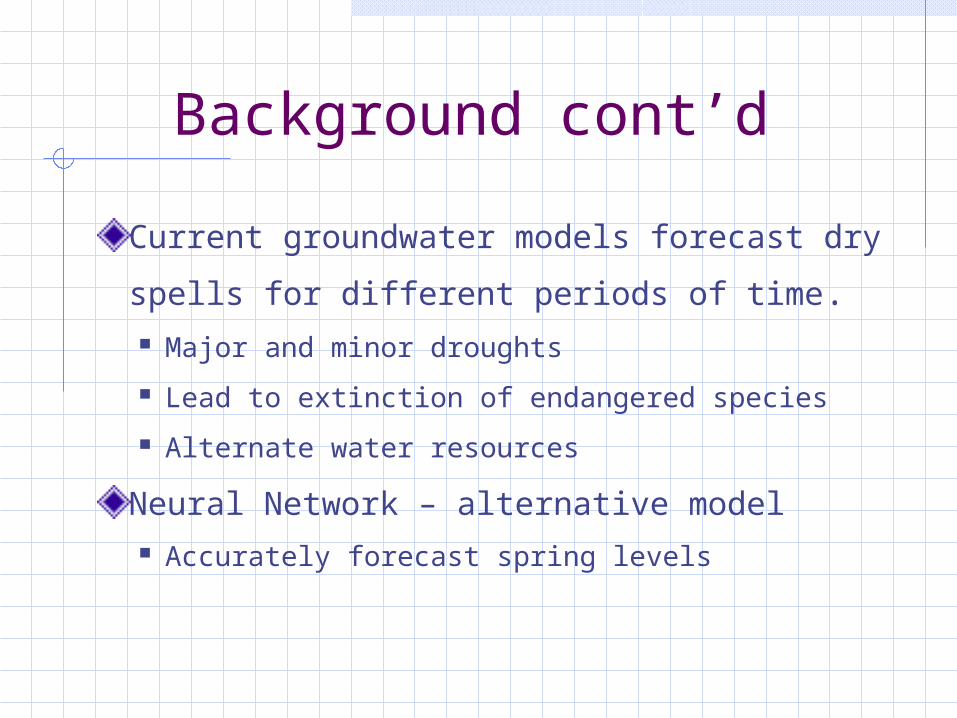
Background cont’d

Current groundwater models forecast

dry spells for different periods of time. Major and minor droughts

Lead to extinction of endangered species

Alternate water resources

Neural Network – alternative model Accurately forecast spring levels

Neural Network Modeling

Started in the 60’sKey innovation in the late 80’s: Backpropagation learning algorithmsNumber of applications has grown rapidly in the 90’s especially financial applicationsGrowing number of publications presenting environmental applications

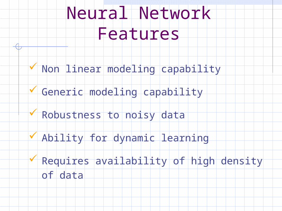
Neural Network Features

Non linear modeling capability

Generic modeling capability

Robustness to noisy data

Ability for dynamic learning

Requires availability of high density of data

Neural Network Forecasting of Spring

Levels

Philippe Tissot - 2000

H (t+i)

Output LayerHidden Layer

Precipitation 1 History

Baseflow History

Precipitation 3 History

Precipitation 2 History

Input Layer

Spring Level Forecast

(a1,ixi)

b1

b2

(X1+b1)

b3

(X2+b2)

(X3+b3)

(a2,ixi)

(a3,ixi)

Data

Daily baseflow and precipitation data

spanning 50 years (01/01/1950-12/31/2000)

HYSEP – separated streamflow data into

baseflow and surface runoff components

Separate into 5 sets of 10 years

Train on 1 set and test on other 4

Compare results to persistence model

Neural Network Design Strategy

Find optimum number of previous days

of baseflow as inputs to model.

Find optimum number of previous days

of precipitation as inputs to model.

Find how many neurons provide the

best neural network performance.

Target Error Criterion and Root Mean Square Error

Target Error Criterion – percentage of model’s results that fall within 20% of the measured baseflow values

Root Mean Square Error (RMSE) – overall error of a sampling distribution of a group with n cases in a group

Target Error Criterion with Increasing Previous Baseflow Days

82 %

84 %

86 %

88 %

90 %

92 %

94 %

0 10 20 30 40 50 60

# of Days

Tar

get

Err

or

Cri

teri

on

(20

%)

10-Day Forecast

30-Day Forecast

RMSE with Increasing Previous Baseflow Days

0

5

10

15

20

25

30

35

40

0 10 20 30 40 50 60

# of Days

RM

SE

(cf

s)

10-Day Forecast

30-Day Forecast

Target Error Criterion with Addition of Precipitation Station

84 %85 %86 %87 %88 %89 %90 %91 %92 %93 %94 %

0 10 20 30 40 50 60

# of Days

Tar

get

Err

or

Cri

teri

on

(20

%)

10-Day Forecast

30-Day Forecast

RMSE with Addition of Precipitation Station

0

5

10

15

20

25

30

35

40

0 10 20 30 40 50 60

# of Days

RM

SE

(cf

s)

10-Day Forecast

30-Day Forecast

Target Error Criterion with Increasing Neurons in Hidden Layer

82 %

84 %

86 %

88 %

90 %

92 %

94 %

96 %

0 0.5 1 1.5 2 2.5 3 3.5 4 4.5# of Neurons

Tar

get

Err

or

Cri

teri

on

(20

%)

10-Day Forecast

30-Day Forecast

RMSE with Increasing Neurons in Hidden Layer

0

50

100

150

200

250

0 1 2 3 4 5

# of Neurons

RM

SE

(cf

s)

10-Day Forecast

30-Day Forecast

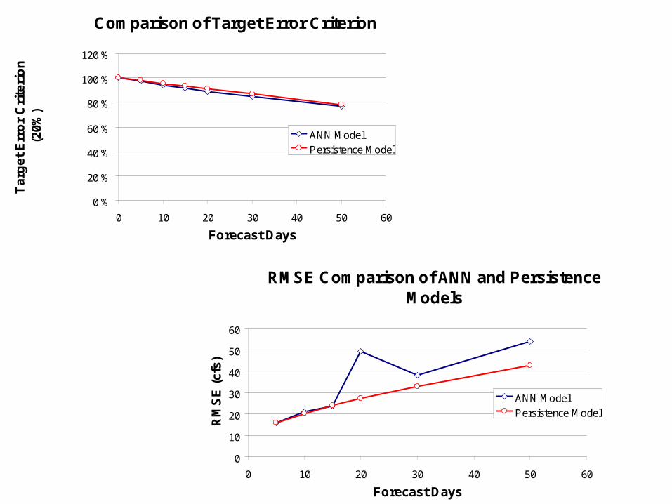
Comparison of Target Error Criterion

0 %

20 %

40 %

60 %

80 %

100 %

120 %

0 10 20 30 40 50 60

Forecast Days

Tar

get

Err

or

Cri

teri

on

(2

0%)

ANN Model

Persistence Model

RMSE Comparison of ANN and Persistence Models

0

10

20

30

40

50

60

0 10 20 30 40 50 60

Forecast Days

RM

SE

(cf

s)

ANN Model

Persistence Model

Good Example

Days in Test Set

Base

flow

(cf

s)

Measured BaseflowANN Forecast

Bad Example – Too many spikes

Days in Test Set

Base

flow

(cf

s)

Measured BaseflowANN Forecast

Comparison of Target Error Criterion and RMSE through Neural Network

Design Process

10-Day Optimization 30-Day OptimizationBaseflow 93.28 84.60

Precipitation 93.48 84.55Neurons 94.30 85.29

Persistence 95.62 86.93

Target Error Criterion

10-Day Optimization 30-Day OptimizationBaseflow 21.83 34.73

Precipitation 21.58 35.23Neurons 20.01 67.03

Persistence 20.19 32.99

RMSE

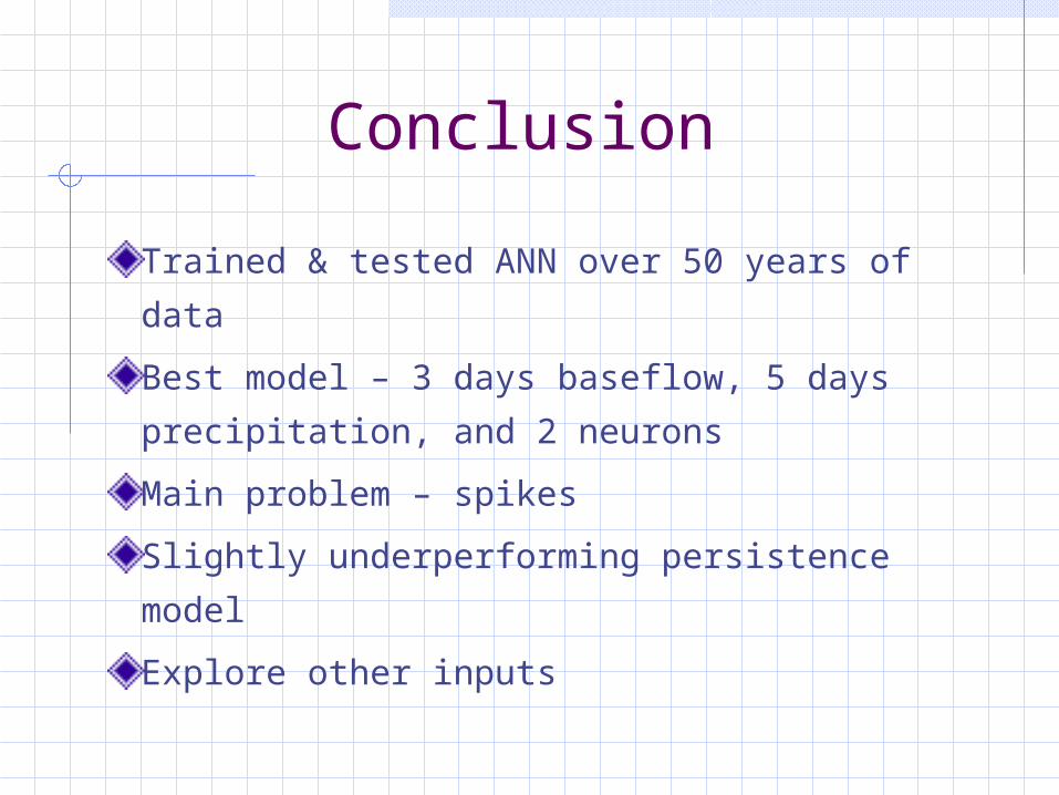
Conclusion

Trained & tested ANN over 50 years of data

Best model – 3 days baseflow, 5 days

precipitation, and 2 neurons

Main problem – spikes

Slightly underperforming persistence model

Explore other inputs

Questions