Embed Size (px)
Citation preview
David Laibson
Harvard University
Princeton Conference
on Consumption and Finance
February 20, 2014
14
HRS: In 2008, the median holding of
financial assets is $12,500
among 1-person households
HRS: In 2008, the median holding of
financial assets is $111,600
among 2-person households
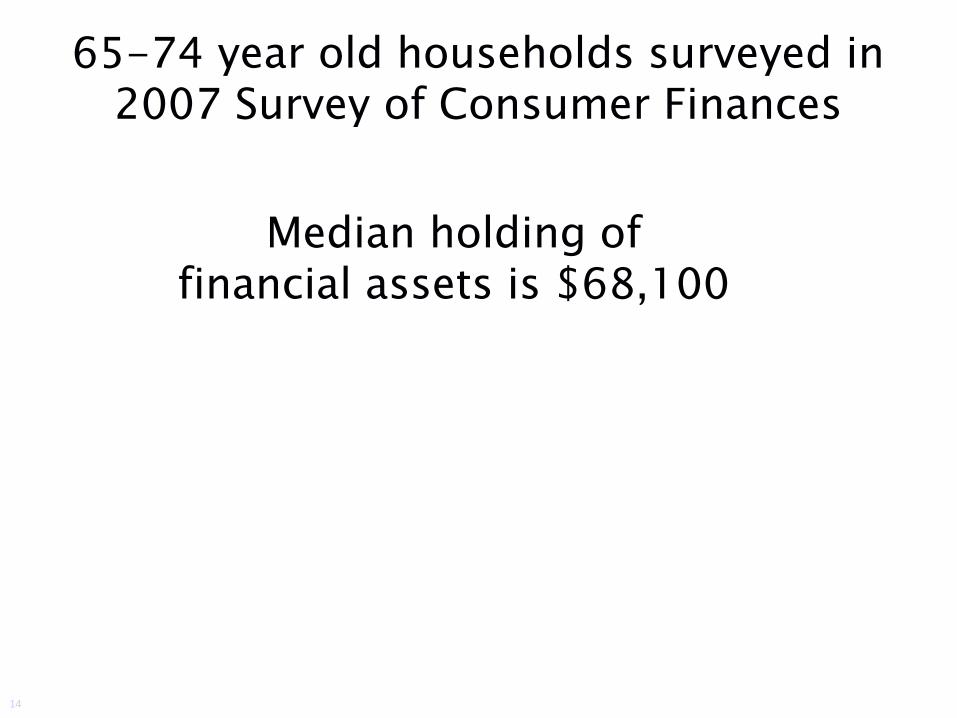
65-74 year old households surveyed in 2007 Survey of Consumer Finances
Median holding of financial assets is $68,100
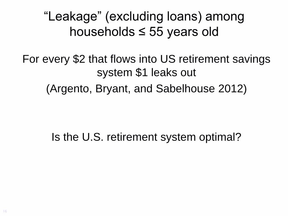
“Leakage” (excluding loans) among
households ≤ 55 years old
For every $2 that flows into US retirement savings
system $1 leaks out
(Argento, Bryant, and Sabelhouse 2012)
Is the U.S. retirement system optimal?
16

Present-biased discounting Strotz (1957), Phelps and Pollak (1968), Elster (1989),
Akerlof (1992), Laibson (1997), O’Donoghue and Rabin (1999)
Current utils get full weight
Future utils weighted βδt
ut + βδut+1 + βδ2ut+2 + βδ3ut+3 + βδ4ut+4+ …
ut + β[ δut+1 + δ2ut+2 + δ3ut+3 + δ4ut+4 + … ]
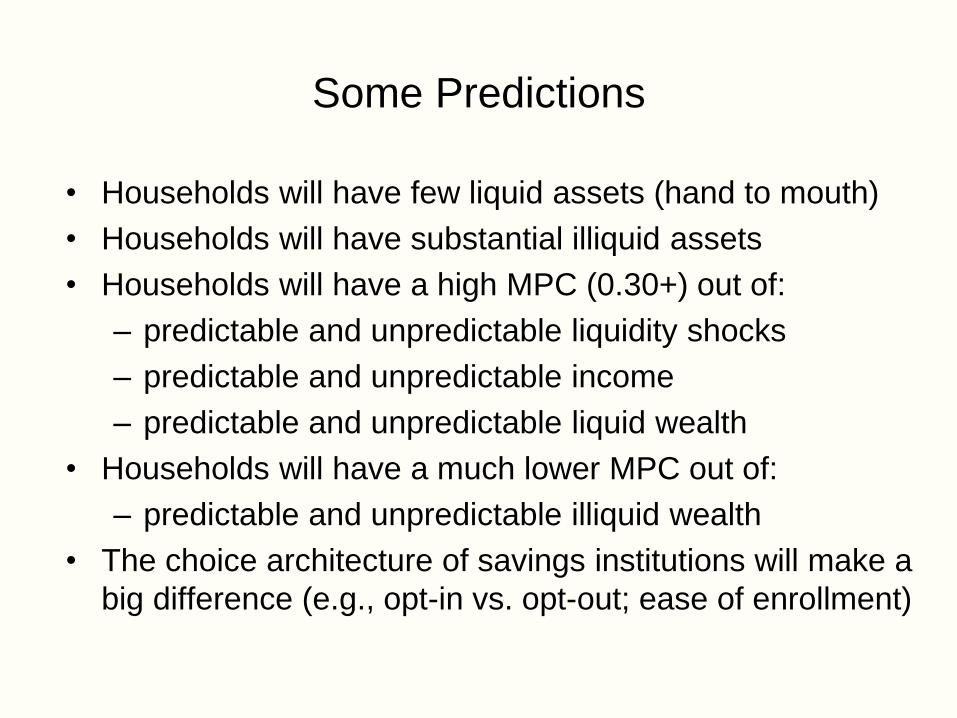
Some Predictions
• Households will have few liquid assets (hand to mouth)
• Households will have substantial illiquid assets
• Households will have a high MPC (0.30+) out of:
– predictable and unpredictable liquidity shocks
– predictable and unpredictable income
– predictable and unpredictable liquid wealth
• Households will have a much lower MPC out of:
– predictable and unpredictable illiquid wealth
• The choice architecture of savings institutions will make a
big difference (e.g., opt-in vs. opt-out; ease of enrollment)

Households live hand to mouth Lusardi and Tufano (2009)
How confident are you that you could come up with
$2,000 if an unexpected need arose within the next
month?
– I am certain…I could
– I could probably…
– I probably could not…
– I am certain…I could not
– Do not know.
24
47%
53%
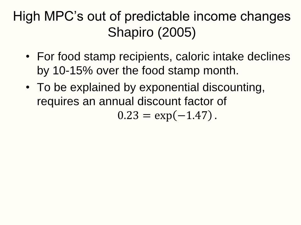
High MPC’s out of predictable income changes
Shapiro (2005)
• For food stamp recipients, caloric intake declines
by 10-15% over the food stamp month.
• To be explained by exponential discounting,
requires an annual discount factor of
0.23 = exp −1.47 .
High MPC’s out of Social security
Mastrobuoni and Weinberg (2009)
• Individuals with substantial savings smooth
consumption over the monthly pay cycle
• Individuals without savings consume 25 percent
fewer calories the week before they receive SS
checks relative to the week after

Lifecycle simulations (Angeletos et al 2001)
• Mortality
• Dependents
• Retirement/Social Security
• Three educational groups: NHS, HS, COLL
• Stochastic labor income
• Credit limit: (.30)(permanent income)
• 3 state variables: liquid and illiquid wealth, income.
• 2 choice variables: liquid and illiquid wealth investment
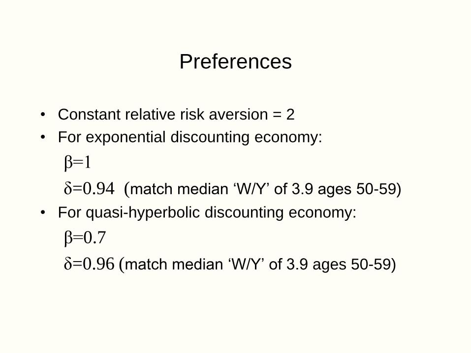
Preferences
• Constant relative risk aversion = 2
• For exponential discounting economy:
β=1
δ=0.94 (match median ‘W/Y’ of 3.9 ages 50-59)
• For quasi-hyperbolic discounting economy:
β=0.7
δ=0.96 (match median ‘W/Y’ of 3.9 ages 50-59)
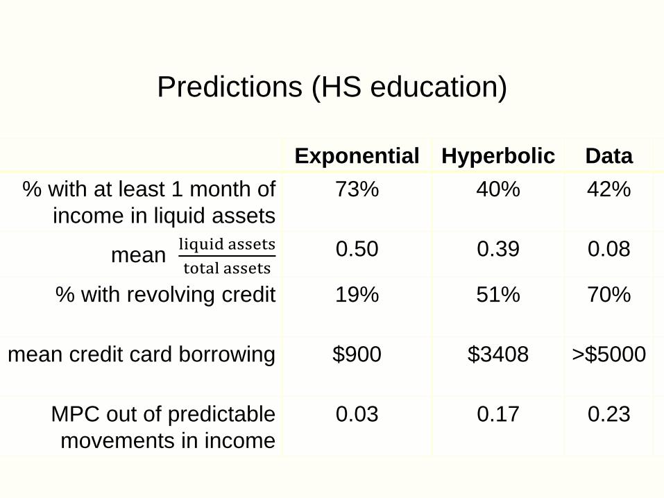
Predictions (HS education)
Exponential Hyperbolic Data
% with at least 1 month of
income in liquid assets
73% 40% 42%
mean liquid assets
total assets 0.50 0.39 0.08
% with revolving credit
19% 51% 70%
mean credit card borrowing
$900 $3408 >$5000
MPC out of predictable
movements in income
0.03 0.17 0.23
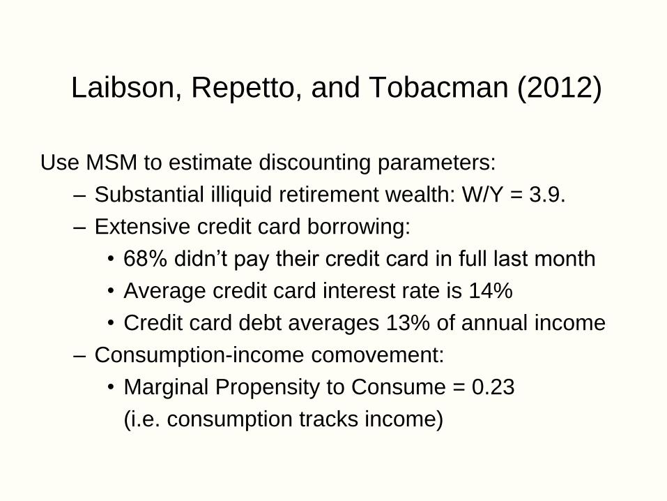
Laibson, Repetto, and Tobacman (2012)
Use MSM to estimate discounting parameters:
– Substantial illiquid retirement wealth: W/Y = 3.9.
– Extensive credit card borrowing:
• 68% didn’t pay their credit card in full last month
• Average credit card interest rate is 14%
• Credit card debt averages 13% of annual income
– Consumption-income comovement:
• Marginal Propensity to Consume = 0.23
(i.e. consumption tracks income)

LRT Results:
Ut = ut + b [dut+1 + d2ut+2 + d3ut+3 + ...]
b = 0.70 (s.e. 0.11)
d = 0.96 (s.e. 0.01)
Null hypothesis of b = 1 rejected (t-stat of 3).
Specification test accepted.
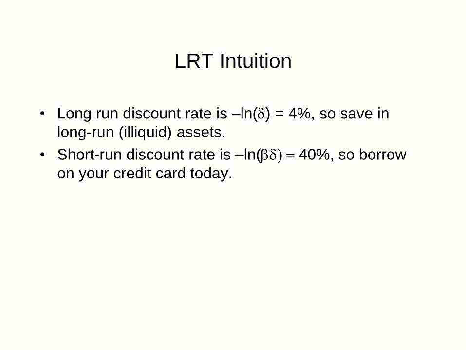
LRT Intuition
• Long run discount rate is –ln(d) = 4%, so save in
long-run (illiquid) assets.
• Short-run discount rate is –ln(bd) = 40%, so borrow
on your credit card today.

Strotz (1957)
Thaler and Shefrin (1981)
Schelling (1984)
Ainslie (1992)
Laibson (1997)
Wertenbroch (1998)
Laibson, Repetto, Tobacman (1998)
Angeletos et al. (2001)
Gul and Pesendorfer (2001)
Ariely and Wertenbroch (2002)
Ashraf, Karlan, and Yin (2006)
Amador, Werning, and Angeletos (2006)
Fudenberg and Levine (2006)
Karlan, Gine, and Zinman (2009)
Kauer, Kremer, and Mullainathan (2010)
Houser, Schunk, Winter and Xiao (2010)
Royer, Stehr, and Sydnor (2011)
Alsan, Armstrong, Beshears, Choi, del Rio, Laibson, Madrian, Marconi (2011)
Homer (700 BC): “If you supplicate your men and implore them to set you free, then they must tie you fast with even more lashings.”

Ashraf, Karlan, and Yin (2006)
• Offered a commitment savings product to
randomly chosen clients of a Philippine bank
• 28.4% take-up rate of commitment product
(either date-based goal or amount-based
goal)
• Subjects with more present-bias are more
likely to take up the product
• After twelve months, average savings
balances increased by 81% for those clients
assigned to the treatment group relative to
those assigned to the control group.
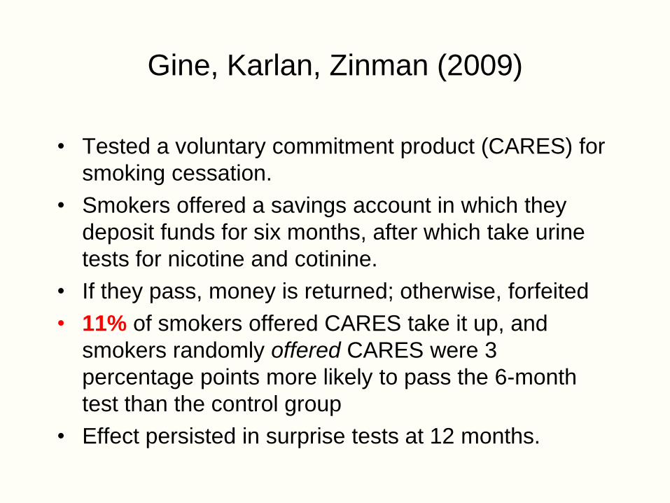
Gine, Karlan, Zinman (2009)
• Tested a voluntary commitment product (CARES) for
smoking cessation.
• Smokers offered a savings account in which they
deposit funds for six months, after which take urine
tests for nicotine and cotinine.
• If they pass, money is returned; otherwise, forfeited
• 11% of smokers offered CARES take it up, and
smokers randomly offered CARES were 3
percentage points more likely to pass the 6-month
test than the control group
• Effect persisted in surprise tests at 12 months.
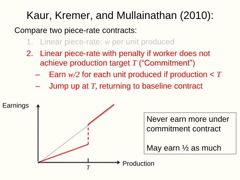
Kaur, Kremer, and Mullainathan (2010):
Compare two piece-rate contracts:
1. Linear piece-rate: w per unit produced
2. Linear piece-rate with penalty if worker does not
achieve production target T (“Commitment”)
– Earn w/2 for each unit produced if production < T
– Jump up at T, returning to baseline contract
T
Earnings
Production
Never earn more under
commitment contract
May earn ½ as much
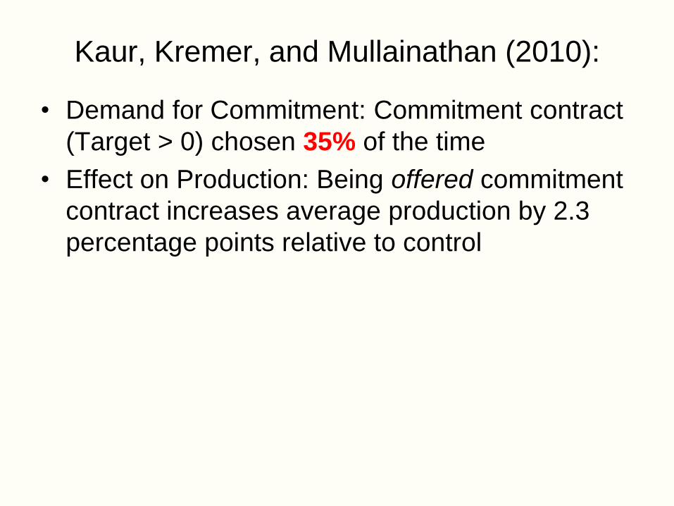
Kaur, Kremer, and Mullainathan (2010):
• Demand for Commitment: Commitment contract
(Target > 0) chosen 35% of the time
• Effect on Production: Being offered commitment
contract increases average production by 2.3
percentage points relative to control

What are the features that make a savings account attractive?
Liquidity?
Illiquidity? ◦ Present-biased preferences
If people like illiquidity, what kind of illiquidity is most effective? ◦ 10% penalty?
◦ 20% penalty?
◦ Complete illiquidity?

Freedom Account Goal Account
Liquid - can withdraw money
any time within the period of
experiment (1 year)
22% interest per year
Subject picks a goal date
Illiquid before goal date
10% early withdrawal penalty
Liquid after goal date, just like
freedom account
22% interest per year
What does illiquid mean? Three cases that we study: • 10% withdrawal penalty: you get $ but your account is debited (1.1)$. • 20% withdrawal penalty: you get $ but your account is debited (1.2)$. • No withdrawals
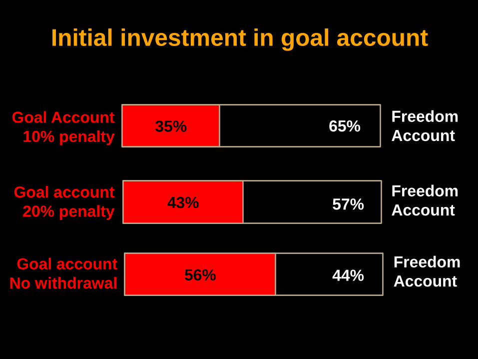
Initial investment in goal account
Freedom
Account
Freedom
Account
Freedom
Account
Goal Account
10% penalty
Goal account
20% penalty
Goal account
No withdrawal
35% 65%
43% 57%
56% 44%
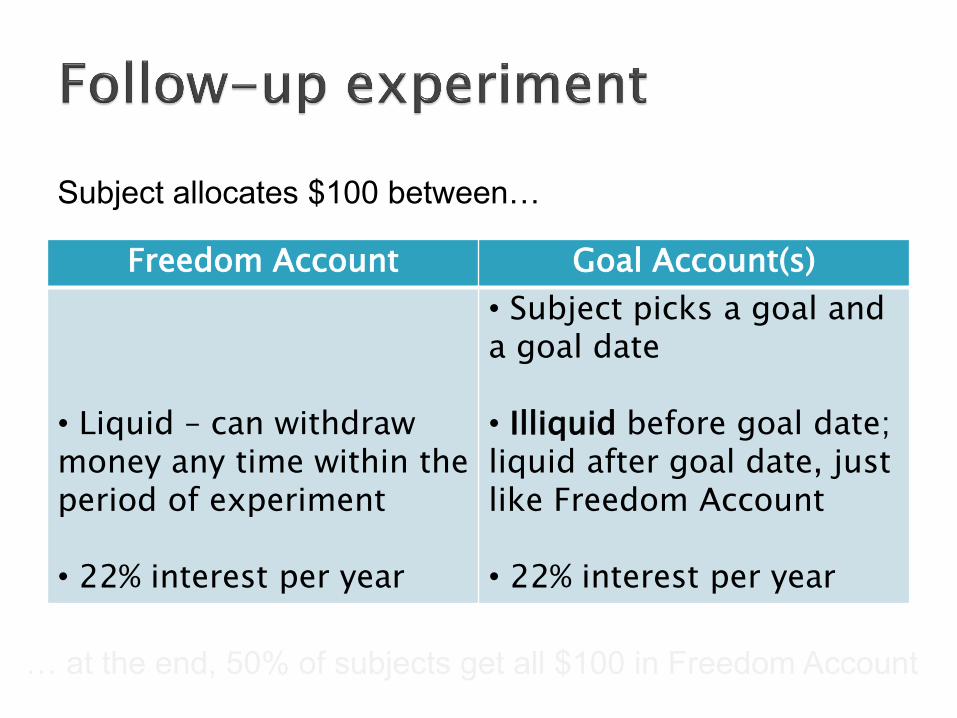
Freedom Account Goal Account(s)
• Liquid – can withdraw money any time within the period of experiment
• 22% interest per year
• Subject picks a goal and a goal date
• Illiquid before goal date; liquid after goal date, just like Freedom Account
• 22% interest per year
Subject allocates $100 between…
… at the end, 50% of subjects get all $100 in Freedom Account

Goal Account characteristics
Arm 1 10% Penalty before goal date
Arm 2 No Withdrawal before goal date
Arm 3 • 10% Penalty • No Withdrawal
Arm 4 Safety Valve – no withdrawal before goal date, except in case of a financial emergency as determined by the subject
Two goal accounts
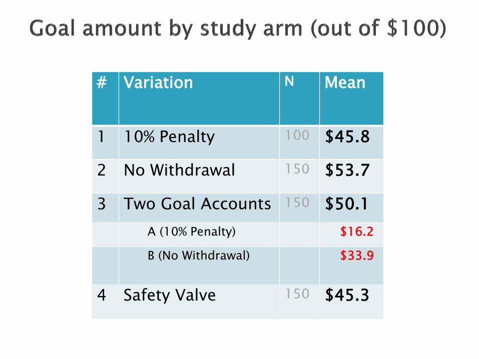
# Variation N Mean
1 10% Penalty 100 $45.8
2 No Withdrawal 150 $53.7
3 Two Goal Accounts 150 $50.1
A (10% Penalty) $16.2
B (No Withdrawal) $33.9
4 Safety Valve 150 $45.3
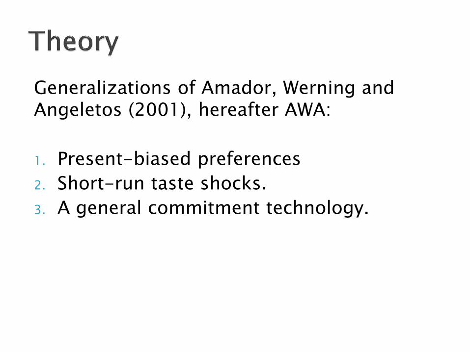
Generalizations of Amador, Werning and Angeletos (2001), hereafter AWA:
1. Present-biased preferences
2. Short-run taste shocks.
3. A general commitment technology.
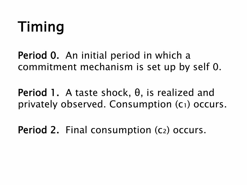
Timing
Period 0. An initial period in which a commitment mechanism is set up by self 0.
Period 1. A taste shock, θ, is realized and privately observed. Consumption (c₁) occurs.
Period 2. Final consumption (c₂) occurs.
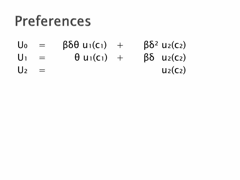
U₀ = βδθ u₁(c₁) + βδ² u₂(c₂)
U₁ = θ u₁(c₁) + βδ u₂(c₂)
U₂ = u₂(c₂)
c2
c1
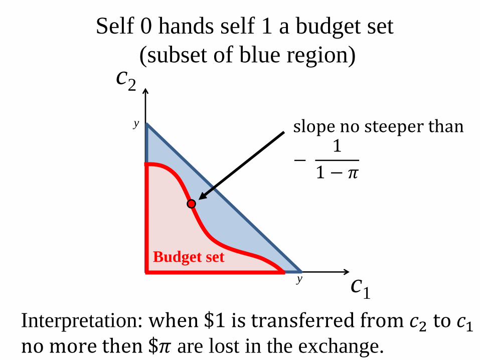
Self 0 hands self 1 a budget set
(subset of blue region)
Budget set
y
y
Interpretation: when $1 is transferred from 𝑐2 to 𝑐1 no more then $𝜋 are lost in the exchange.
slope no steeper than
− 1
1 − 𝜋

c2
c1
)* *
1 2,c c
* *
1 2c c+
)* *
1 2 1c c +
slope = -1
1slope =
1
Two-part budget set
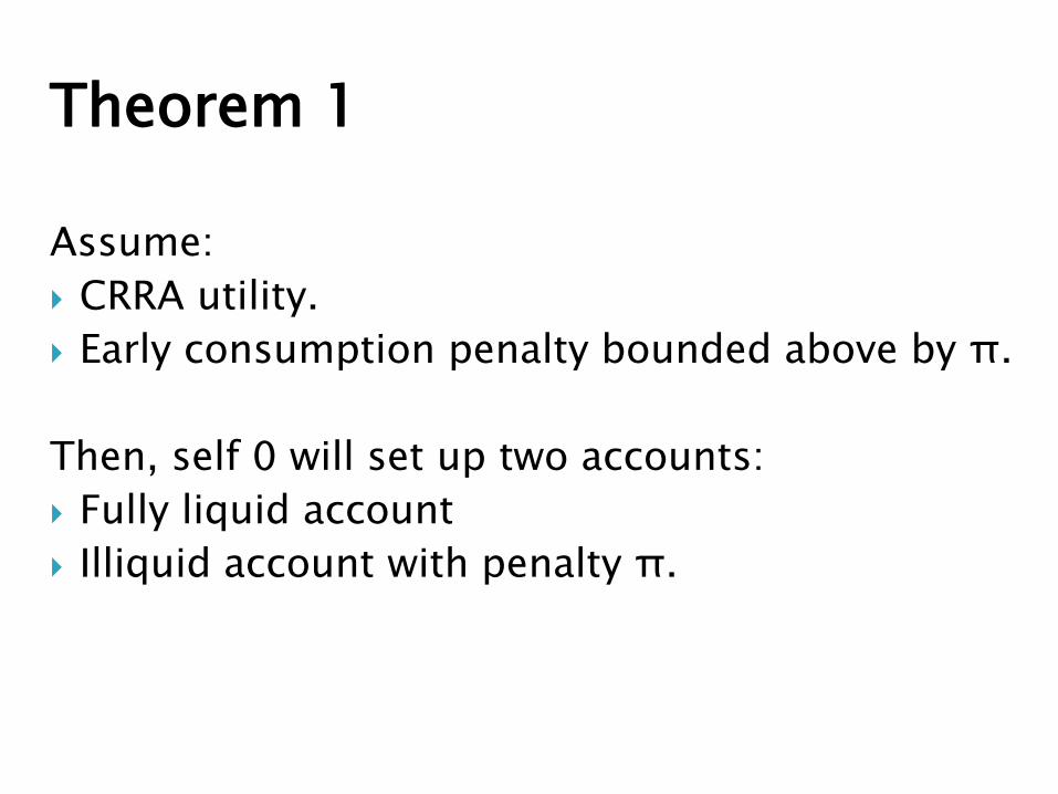
Theorem 1 Assume:
CRRA utility.
Early consumption penalty bounded above by π.
Then, self 0 will set up two accounts:
Fully liquid account
Illiquid account with penalty π.
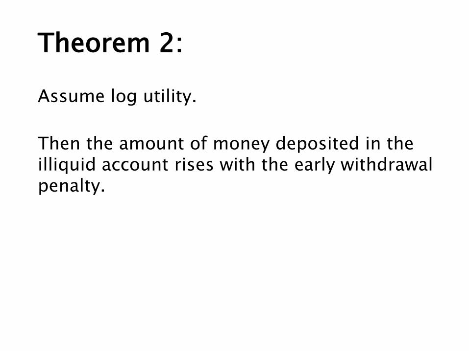
Theorem 2:
Assume log utility.
Then the amount of money deposited in the illiquid account rises with the early withdrawal penalty.

Initial investment in goal account
Freedom
Account
Freedom
Account
Freedom
Account
Goal Account
10% penalty
Goal account
20% penalty
Goal account
No withdrawal
35% 65%
43% 57%
56% 44%
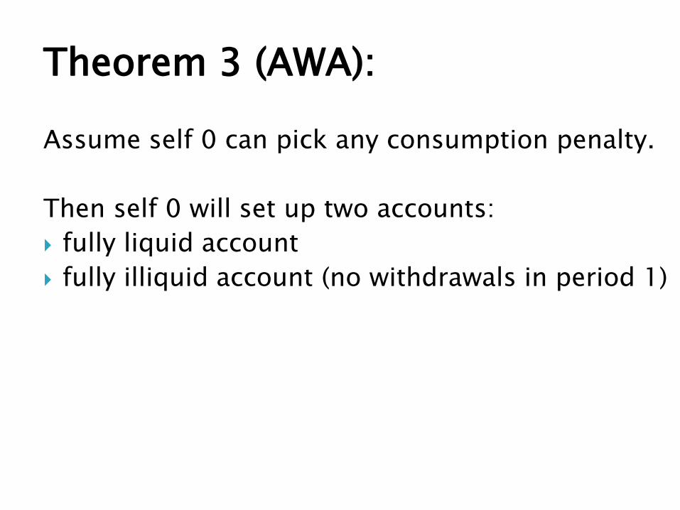
Theorem 3 (AWA):
Assume self 0 can pick any consumption penalty.
Then self 0 will set up two accounts:
fully liquid account
fully illiquid account (no withdrawals in period 1)
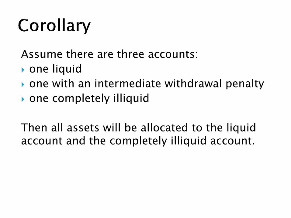
Assume there are three accounts:
one liquid
one with an intermediate withdrawal penalty
one completely illiquid
Then all assets will be allocated to the liquid account and the completely illiquid account.
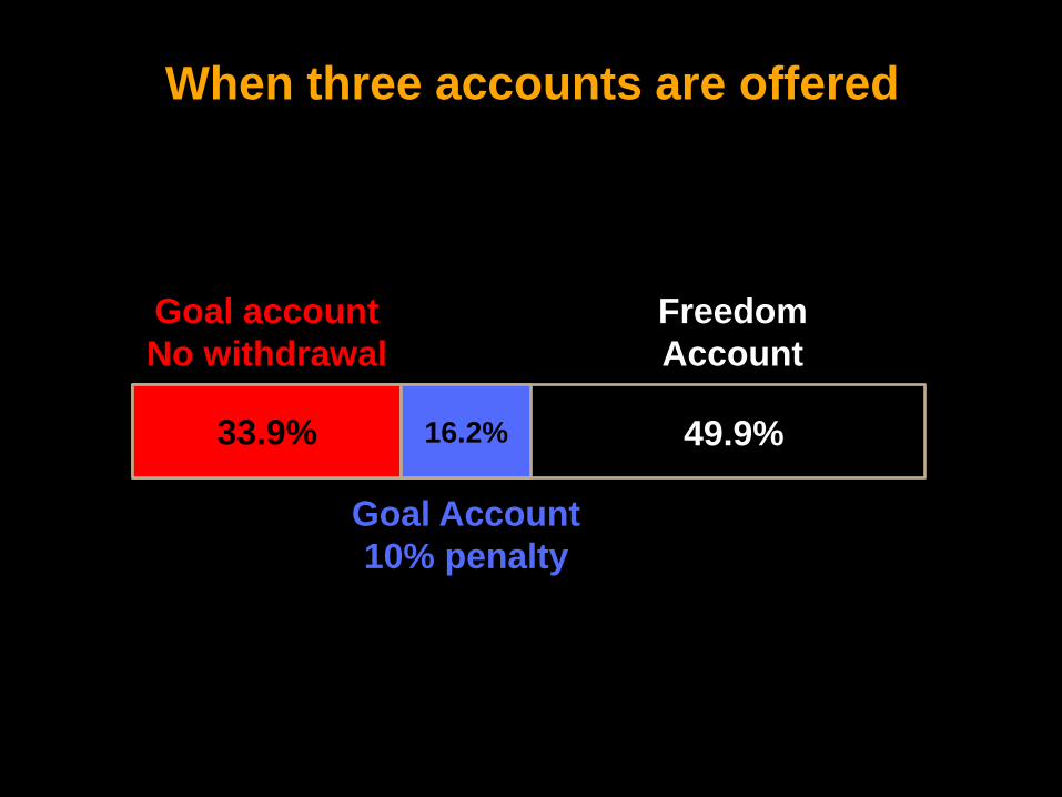
When three accounts are offered
Freedom
Account
Goal account
No withdrawal
33.9% 49.9% 16.2%
Goal Account
10% penalty
House money vs. own money
Interest rates
Demand effect (?)
Stakes
Short-run vs. Long-run
Trust
Menus
Why do people dislike penalty-based schemes?

Potential implications for the design of a retirement saving system?
Theoretical framework needs to be generalized: 1. Allow penalties to be transferred to other agents
2. Heterogeneity in sophistication/naivite
3. Heterogeneity in present-bias
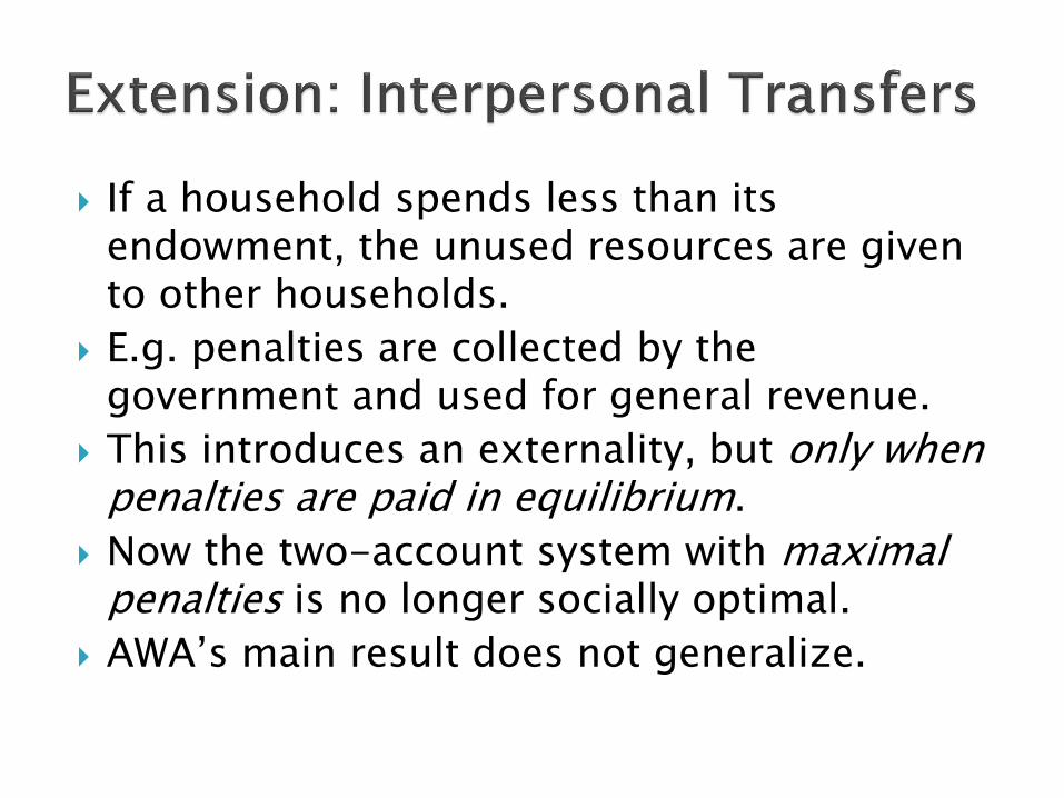
If a household spends less than its endowment, the unused resources are given to other households.
E.g. penalties are collected by the government and used for general revenue.
This introduces an externality, but only when penalties are paid in equilibrium.
Now the two-account system with maximal penalties is no longer socially optimal.
AWA’s main result does not generalize.
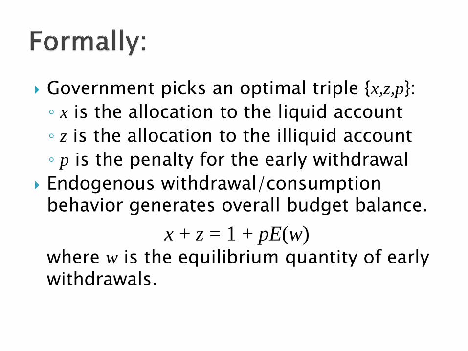
Government picks an optimal triple {x,z,p}:
◦ x is the allocation to the liquid account
◦ z is the allocation to the illiquid account
◦ p is the penalty for the early withdrawal
Endogenous withdrawal/consumption behavior generates overall budget balance.
x + z = 1 + pE(w) where w is the equilibrium quantity of early withdrawals.

15
20
25
30
35
40
45
50
0.6 0.65 0.7 0.75 0.8
CRRA = 2 CRRA = 1
Present bias parameter: β

The optimal penalty almost eliminates early withdrawals.
◦ This engenders an asymmetry: better to set the penalty above its optimum then below its optimum.
Welfare losses are in (1- 𝛽)2.
◦ Getting the penalty right for low 𝛽 agents has much greater welfare consequences than getting it right for high 𝛽 agents.

Expected Utility Given A Fixed Penalty Level: β=0.6
Penalty for Early Withdrawal

Expected Utility Given A Fixed Penalty Level: β=0.1
Penalty for Early Withdrawal
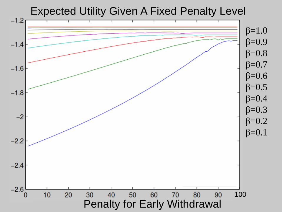
Expected Utility Given A Fixed Penalty Level
Penalty for Early Withdrawal 100
β=1.0
β=0.9
β=0.8
β=0.7
β=0.6
β=0.5
β=0.4
β=0.3
β=0.2
β=0.1

Once you start thinking about low β households, nothing else matters.

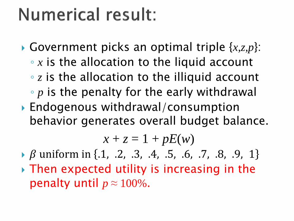
Government picks an optimal triple {x,z,p}:
◦ x is the allocation to the liquid account
◦ z is the allocation to the illiquid account
◦ p is the penalty for the early withdrawal
Endogenous withdrawal/consumption behavior generates overall budget balance.
x + z = 1 + pE(w) 𝛽 uniform in .1, .2, .3, .4, .5, .6, .7, .8, .9, 1
Then expected utility is increasing in the penalty until p ≈ 100%.

Our three-period model and experimental evidence imply that optimal retirement systems have highly illiquid retirement accounts.
Good news: Almost all countries in the world have a system like this: A public social security system plus illiquid supplementary retirement accounts (either DB or DC or both).
Bad news: The U.S. doesn’t – our defined contribution retirement accounts are essentially liquid.