David A. Patterson, Garth Gibson and Randy H. Katz “A case for redundant arrays of inexpensive disks (RAID)”,

SIGMOD’88 Pages 109 – 116.

I/O Parallelism Enabled by Controllers embedded in Disks

• Mainframe disk controllers were at one time not incorporated into disks

• In late 1980’s, disk vendors were embedding controllers in each disk and using single chip DMA interfaces

• Use of many inexpensive disks with independent controllers were correctly thought to hold promise of increased transfer bandwidth and lower cost

• See Figure 1 [Patterson88]

Performance Issues for Large and Small Data Transfers

• Applications make varying size I/O requests– OLAP, data mining, scientific applications, backups carry out

large data transfers

– Small requests are associated with transaction processing, but also occur in most types of codes, including in codes where many small requests could be, but are not, aggregated into large requests

• Figure 2 in [Patterson88] depicts idealized RAID performance characteristics – Group large transfers over many disks for bandwidth

– Small transfers go to single disk to minimize seek overheads

Level 1 RAID

• Mirrored disks– all disks duplicated, write to data disk and write to check disk

• D - total disks with data

• G - number of disks in group (not including check disks)

• C - check disks in group

– Total number disks 2D

– Overhead 100%

– Useful storage capacity 50%

• Events/second v.s. single disk, efficiency per disk– All reads – 2D, 1.0

– All writes – D, 0.5

– All read/modify/write 4D/3, 0.67

2nd Level Raid

• Hamming code for Error Correction

• Bit interleave data

• Add check disks to dtected and correct single errors

• Read requires reading sector from each of G+C disks

• Write involves read/modify/write cycle to each of G+C disks

• For G=10, C=4

• Number disks 1.4D, Overhead 40%, Usable storage 71%

2nd level RAID continued

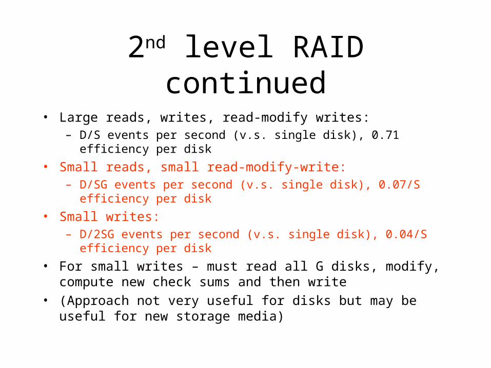
• Large reads, writes, read-modify writes:– D/S events per second (v.s. single disk), 0.71 efficiency per disk

• Small reads, small read-modify-write:– D/SG events per second (v.s. single disk), 0.07/S efficiency per disk

• Small writes:– D/2SG events per second (v.s. single disk), 0.04/S efficiency per disk

• For small writes – must read all G disks, modify, compute new check sums and then write

• (Approach not very useful for disks but may be useful for new storage media)

3rd Level RAID

• Assume that disk controllers detect errors –– Single check disk/group

• Check information at end of each sector used to correct soft errors• Reduce check disks to one per group• Example G=10• Number disks 1.1D, Overhead cost 10%, usable storage capacity 91%• Large reads, large writes, large read-modify-write

– D/S events/second (v.s. single disk), 0.91/S efficiency

• Small reads, small read-modify-writes– D/SG events/second (v.s. single disk), 0.09/S efficiency

• Small writes– D/2SG events/second (v.s. single disk), 0.05/S efficiency

4th Level Raid

• Get rid of bit-interleaving

• Information at end of sector is used to correct errors

• Read can access a single sector

• Write requires 4 accesses – 2 reads, 2 writes– New parity = (old data xor new data) xor old parity

• Why? If olddata[I] = newdata[I] then olddata[I] xor newdata[I] = 0. Parity is unchanged so 0 xor oldparity[I] is correct

• If olddata[I] is not equal to newdataa[I], parity changes

• Olddata[I] xor newdata[I] = 1 and 1 xor oldparity[I] is the complement of oldparity[I]

4th level RAID

• G=10

• Number disks 1.1D, overhead cost 10%, usable storage 91%

• Large reads, writes, read-modify-writes – D/S events/sec (v.s. single disk), 0.91/S efficiency

• Small reads, small read-modify-write – D/G events/sec (v.s. single disk), 0.09 efficiency

• Small writes– D/2G events/sec (v.s. single disk), 0.05 efficiency

• Single check disk is bottleneck

5th level RAID

• No single check disk• Distribute data and check info across all disks• G =10• Number disks 1.1D, Overhead costs 10%, usable storage

91%• Large reads, writes, read-modify,writes• D/S events/sec, 0.91 efficiency• Small reads: (1+C/G)D events/second, 1.0 efficiency• Small writes: (1+C/G)D/4 events/second, 0.25 efficiency• Small read-modify-writes: (1+C/G)D/2 events/second, 0.50

efficiency

Comparison of RAID 1-5

• Figure 3 [Patterson88]– Compares RAID 1-4 schemes

– Note that in RAID 4, check information is calculated over piece of each transfer unit and is placed into single sector

• Figure4 [Patterson88]– Schematically depicts reason for performance advantage of RAID

5

– Check information and data are spread evenly throughout the disks

J. Wilkes, R. Golding, C. Staelin and T. Sullivan

The HP AutoRAID hierarchical storage system

Pages 96 – 108, ACM Symposium on Operating System Principals, 1995

Motivation

• Combination Raid 1, Raid 5 -- efficient use of storage v.s. performance– write-active data are mirrored to optimize performance

– write-inactive data are stored in RAID 5 for best cost-capacity

– large sequential writes also go to RAID 5

• Lots of detailed parameter tweaking involved in setting up a disk array -- idea is to automate this as well as to create a system that adapts to changes in workload, amount of data stored– space is stored mirrored when there is lots of space

– inactive data is migrated to RAID 5 as space grows scarcer

• Log structured Raid 5 writes

Architecture

• Figure 2 [Wilkes95] depicts architecture– Set of disks

– Intelligent controller that incorporates a microprocessor

– Mechanisms for calculating parity, volatile and non-volatile caches for staging data

– Connection to one or more host computers

– Speed matching buffers

• Array presents one or more SCSI logical units (LUN) to host– Host uses SCSI command set to interact with disk array

Datastructures

• Combination RAID 1, RAID 5• Data space on disks broken into large granularity objects --

Physical EXtents (PEXes) -- (e.g. 1 MB size)• Several PEXes combined to form PEG -- Physical Extent

Group– PEG can be assigned to mirrored class, RAID 5 class or be unassigned

– PEG includes at least 3 PEXes on different disks

– PEXes are allocated to PEGs to balance amount of data on disks, retain redundancy guarantees

• A segment is a subset of a PEX (e.g. each PEX divided into 8 128KB segments)

Datastructures

• Stripe is a row of data and parity segments in a RAID 5 storage class

• Space visible to clients divided into Relocation Blocks (RBs)– Relatively small (e.g. 64K ) units -- basic unit of migration– When SCSI logical unit (LUN) is createdor increased in size,

address space mapped into set of RBs– RB not assigned space in a particular PEG until host issues a write

to a LUN address that maps to the RB– Each PEG can hold many RBs - number being function of PEG’s

size and storage class

• See Fig 2, 3 [Wilkes95]

Mapping Structures

• Virtual device tables -- one per LUN– list of RBs and pointers to the PEGs in which they

reside

• PEG tables– one per PEG. Holds list of RBs in PEG and list of

PEXes used to store them

• PEX tables – one per physical disk drive

• See Figure 5 [Wilkes95]

Normal Operations• Host sends SCSI command descriptor block (CDB) to array,

where it is parsed by the controller

• 32 CDBs active, FIFO with 2048 CDBs queued

• If request is a read, data in controller’s cache, data sent to host– otherwise, space allocated in front end buffer cache, one or more read

requests are dispatched to back-end storage classes

• Host can write to nonvolatile (NVRAM) front-end write buffer. Once write is done, host can consider request complete– check to see if cached data needs to be invalidated– allocate space– if space is not available, claim space by flushing dirty data to back-end

storage class

Reads and Writes

• Mirrored– Read call picks one of the copies and issues request to associated disk

– Back-end write call causes write to two disks; returns only when both copies have been updated

• Raid 5 reads and writes– RAID 5 storage laid out as a log

– Freshly “demonted” RBs are appended to the end of a “current RAID 5 write PEG”

– writes can be done in batched mode (more efficient) or per-RB

– read-modify write can also be used in which old data and parity are read, new parity calculated and new parity, new data written to disk

Per-RB writes

• As soon as RB is written, it is flused to disk

• Copy of contents flows past parity detection hardware which carries out running computation of parity for the stripe

• Prior contents of parity block are stored in non-volatile memory

• Each data-RB write causes two disk writes, one for data, one for the parity RB

Batched writes

• Parity written only after all data RBs in a stripe have been written, or at the end of a batch– If at the beginning of a batched write, there are already valid data in PEG

– Prior contents of parity block are copied into nonvolatile memory along with index of highest-numbered RB in PEG with valid data

• Parity computed on the fly by the parity calculation logic as each data RB is being wirtten

• If batched wirte fails, system is returned to pre-batch state by restoring old parity and RB index and write is retried using per-RB method

• Requires only one additional parity write for each full strip of data

Migration

• RBs moved between levels– background migration policy moves RBs from mirrored storage to

RAID 5

– Mirrored storage class acquires holes or RB slots when RBs are demoted to RAID 5 storage class

– Holes added to free list and can be used to store new or promoted RBs

– Provide enough RB slots in the mirrored storage class to handle future write burst

– Selected for migration using Least Recently Written type algorithm

Reassignment of PEGS

• If new PEG is needed for RAID 5 and no free PEXes are available, mirrored PEG may be chosen for cleaning– all data migrated out to fill holes in other mirrored PEGs

– PEG reclaimed and reallocated to RAID 5 storage class

– RAID 5 storage class acquires holes when RBs are promoted to mirrored storage class (usually because RBs are updated)

– RAID 5 uses logging so holes cannot be reused directly -- array needs to perform periodic garbage collection

– If RAID 5 PEG containing holes is almost full, disk array performs hole-plugging garbage collection -- RBs are copied from PEG with small number of RBs

Performance Results

• Comparison: All systems used:– HP9000/K400 system with one processor, 512 MB memory

– 12 disks -- 2.0 GB 7,200RPM ST32550 Seagate Barracudas

• HP AutoRAID array– One controller, 24 MB controller data cache connected with two fast-wide

SCSI adaptors

• Data General CLARiiON Series 2000 RAID array with 64MB front-end cache– System configured to use RAID 5

– Only one fast-wide SCSI channel was used, this was said not to be the bottleneck

• Just a Bunch of Disks (JBOD-LVM) with data striped in 4MB chunks

Performance Results

• Macrobenchmarks:– OLTP workload made up of medium-weight transactions run against the

HP AUTORAID array, regular RAID array, JBOD-LVM

– Figure 6a – 6.7GB database – fits entirely within mirrored storage in HP AutoRAID

– Results – HP AutoRAID better than RAID 5 but worse than JBOD-LVM.• Expected as mirrored storage should be faster than RAID 5.

• Writes should be slower in RAID 1 than JBOD-LVM and we see a corresponding performance difference.

– Figure 6b – Performance improves as fraction of database held in mirrored storage increases

Microbenchmarks

• Synthetic workload to drive arrays to saturation

• HP Autoraid used 16MB controller data cache, HP 9000/897 used as host, single fast-wide SCSI used for HP AutoRAID and RAID array tests, JBOD only used 11 disks and did not stripe.

• Figure 7– Random 8K reads – always seek, very poor cache use. RAID hurt by cache.

– Random 8K writes – system driven into disk-limited behavior• See 1:2:4 ratio in I/O per second

• RAID 5 – 4 I/O per update

• HP AutoRAID 2 I/O to mirrored storage

• JBOD 1 write

– Sequential reads/writes • Performance comparable to JBOD

• Reason for poor RAID performance not clear

Mendel Rosenblum and John K. Ousterhout“The design and implementation of a log-structured file system”, Pages 1 – 15,

ACM Symposium on Operating System Principals, 1991.

 

Log structured filesystems

• Files are cached in main memory and increasing memory sizes make caches increasingly effective in satisfying read requests– Optimize for situation where disk traffic dominated by writes

• All new information written to disk in a sequential structure called a log– Write performance optimized by minimizing seeks

– Engenders optimized RAID write performance as small writes are minimized

• Sequence of file system changes in file cache and then write changes to disk in single disk write operation– Information written to disk includes file data blocks, attributes, index

blocks, directories and most other information used to manage file systems

Issues

• How to retrieve information from log

• How to manage free space so large extents of free space are always available for writing new data

Reading files• Index information stored in log to permit random access retrievals --

sequential scans are not needed to retrieve information

• Sprite uses data structures identical to UNIX -- – inode with file’s attributes (type, owner, permissions), plus disk addresses of

first ten blocks of file, plus addresses of indirect blocks

– once inode has been found, number of disk I/Os needed to reqd file is identical in Sprite LFS and Unix FFS.

• Unix -- each inode is at a fixed location on disk; Sprite LFS puts inodes in the log

• Sprite uses inode map to maintain current location of each inode

• inode map is divided into blocks written to the log; fixed checkpoint region on each disk identifieds the locations of all the inode map blocks

• inode maps generally found in cache

Free Space Management• Disk divided into large fixed-size extents called segments• Any given segment is written sequentially from beginning to end

– all live data must be copied out of segment before segment is rewritten

• Log is generated on a segment-by-segment basis so system can collect long-lived data into segments

• Segment cleaning -- process of copying live data out of a segment• Need to identify:

– which blocks of each segment are live

– to which file each block belongs and position of block within a file (needed to update file’s inode to point to new location of block)

• Segments contain summary blocks which list the file number and block number for each block in the segment

• Check liveness -- file’s inode or indirect block can be used to see if appropriate block pointer still refers to block

Segment Cleaning Policies

• When should segment cleaner execute?

• How many segments should it clean at a time?

• Which segments should be cleaned?

• How should live blocks be grouped when they are written out?

Write cost

• Average amount of time disk is busy per byte of new data written

• Expressed as multiple of time required if there were no cleaning overhead, and data would be written at full bandwidth with no seek time or rotational latency– 1.0 is perfect – data coul dbe written at full disk bandwidth and there is no

cleaning overhead

– 10.0 means only 1/10th of disk’s maximum bandwidth is used for writing new data

• For log-structured file system with large segments, seeks and rotational latency are negligible for both writing and cleaning so write cost is the total number of bytes moved to and from the disk divided by the number of those bytes that represent new data

Write cost

• In steady state, cleaner must generate one clean segment for every segment of new data written

• U represents fraction of blocks that are live in segment to be cleaned

• Must read N segments and write out N*u segments of live data (where u is between 0 and 1)

• This creates N(1-u) segments of contiguous free space for new data

• Write cost = total bytes read and written/new data written = (read segs + write live + write new)/new data written = (N + N*u + N*(1-u))/N*(1-u) = 2/(1-u)

• See figure 3 – obviously write cost is much lower if fraction of live blocks in segment is small

Optimizing write cost

• Intuition:– Force disk into bimodal segment distribution in

which most segments are nearly full, a few are empty or nearly empty

– Cleaner can usually reclaim with empty segments

– Seems to be a good way minimizing fraction of live blocks in cleaned segments

Simulation Results and Cost of Cleaning

• Models file system as fixed number of 4KB files

• At each step, simulator overwrites one of the files with new data using one of two patterns– Uniform – each file has equal likelihood of being overwritten

– Hot-and-cold – 10% of files are selected 90% of the time

• Simulator runs until all clean segments are exhausted and then runs the cleaner until a threshold number of clean segments are available

• Cleaners used simple greedy policy that chose least utilized segments to clean

• In Hot-and-cold simulation, live blocks are sorted by age before writing out again to separate long-lived (cold) data from short-lived (hot) data

Results

• Figure 4: Disk capacity utilization v.s. write cost: LFS Uniform– Low disk utilization – segments tend to have fewer live write

blocks as disk capacity utilization decreases

– At 75% overall disk capacity utilization, segments cleaned have utilization of 55%

– At overall disk capacities of under 20%, write cost drops below 2.0 – some cleaned segments have no live blocks at all

– Note that disk capacity utilization is not the same as u – fraction of data still live in segments

Results

• Figure 4: Disk capacity utilization v.s. write cost: Hot-and-col– Varying both the access pattern (hot-and-cold) and policy used to deal

with segments (sort blocks by age before writing out into segments)– Locality and better grouping do not help performance– Segments don’t get cleaned until utilization drops to given threshold– Cold segments don’t get cleaned very often and tie up large numbers of

free blocks for long periods of time• Block that get stuck with a cold segment is in deep freeze for a long time• Figure 5 shows segment utilization distributions with greedy cleaner

– Estimate ratio of cost to benefit of cleaning segments– Benefit – amount of free space generated, time that space is likely to

remain free• Benefit/cost = free space generated*age of data/cost = (1-u)*age/(1+u)• Age is estimated by age of youngest block in segment

Results

• Figure 6 – bimodal distribution – fraction of segments v.s. segment utilization

• Cleaning policy cleans cold segments at about 75% utilization but waits until hot segments reach utilization of about 15%

• Since 90% of writes are to hot files, most segments cleaned are hot

• Figure 7 – major improvement in write cost v.s. disk capacity utilization

Brown, A. and D.A. Patterson. "Towards Maintainability, Availability, and Growth Benchmarks: A Case Study of Software RAID Systems." Proceedings of the 2000 USENIX Annual Technical Conference, San Diego,

CA, June 2000.

Availability Benchmarks

• Performance is nice, but may not be key issue right now

• Benchmarks of RAID implementations to assess availability after faults

• Run workload generator

• Inject faults

• Assess performance, resistance to further faults

• Compare commercial RAID systems -- Linux, Solaris, Windows 2000

Availability

• System’s paranoia with respect to transient errors

• Relative priorities placed on preserving application performance v.s. quickly rebuilding redundancy after a failure

• Implementations treated as black boxes

Availability

• Systems can exist in various degraded states• Assess metrics – performance and fault tolerance• Assess via fault injection• Single fault

– System reaches steady state– Inject fault – e.g. disk sector write error – and see what happens

• Multi-fault– Series of faults and maintenance events designed to mimic real world

events

• Simulations used RAID arrays in which one SCSI disk is replaced by an emulated disk– PC running special software to appear to other devices as a disk drive

Fault model

• Disk faults modeled after those seen in a 368 disk array at UC Berkeley

• Faults recorded over 18 months– Recovered media errors, write failures, hardware errors (such as device

diagnostic failures),SCSI timeouts, SCSI bus-level parity errors

• Categories modeled– Correctable media errors – disk sectors about to go bad

– Uncorrectable media errors – unrecoverably damaged disk sectors

– Hardware errors on any SCSI command

– Parity errors to simulate SCSI bus problems

– Disk hangs to simulate disk firmware bugs/failures during and between SCSI commands

Workload

• SPECWeb99– Uses one or more clients to generate realistic, statistically

reproducible web workload

– Static, dynamic content, form submissions, server-side banner-ad rotation

– Load designed to elicit an aggregate bandwidth from server and measures % of bandwidth actually achieved

– Configured workload to be just short of saturation on all systems • Increased number of active connections until a knee in performance

curve was observed

• Back off load by 5 connections/second

Classification of Results(Figure 2)

• Hits/second v.s. time

• Theoretical minimum number of disk failures that could be tolerated without loosing data

• A – injected fault has no effect

• B – RAID system stops using affected disk. Performance degrades but recovers. Ability to tolerate additional failures does not recover

• C – RAID system reconstructs and after a time recovers ability to tolerate an additional failure– C1 – no performance hit during reconstruction

– C2 – performance hit during reconstruction

• D – System dies

Assessment

• Linux panics easily – reconstructs in cases of transient disk failure

• Solaris and Windows kept faulty disk in service in 7 out of 8 recoverable errors

• Transient errors are very common as are SCSI errors although a defective disk will emit a stream of intermittent transient errors

• Neither are ideal as Linux will lead to unnecessary disk replacement and Windows, Solaris will not recognize when a disk really is going bad

Reconstruction

• RAID-5 volume with one spare– Active disk fails

– Reconstructed using spare

– Spare fails

– Administrator replaces two failed disks

– Reconstruct onto one of the new disks

• Figure 3– Linux reconstructs slowly (1 hour) but with minimal performance hit

during reconstruction

– Solaris reconstructs quickly 10 minutes) but with big performance hit (max of 34% drop)

– Windows is in between – 23 min reconstruction, 18% performance drip

Double Failure

• RAID system experiences disk failure• Reconstruction begins• Live disk is pulled instead of failed disk• In principal, as no data is lost, system should recover when

disk is replaced• Windows did this OK• Linux could not be recovered• Solaris is oblivious – it keeps going even after live disk is

pulled and serves garbage from partially reconstructed spare(!)