Embed Size (px)
Citation preview

Data Warehouse Logical Design
Letizia TancaPolitecnico di Milano
(with the kind support ofRosalba Rossato)

Data Mart logical models
• MOLAP (Multidimensional On-Line Analytical Processing) stores data by using a multidimensional data structure
• ROLAP (Relational On-Line Analytical Processing) uses the relational data model to represent multidimensional data

Data Mart logical modelsData Mart logical modelsMOLAPMOLAP stands for Multidimensional OLAP. In MOLAP cubes the data
aggregations and a copy of the fact data are stored in a multidimensional structure on the computer. It is best when extra storage space is available on the server and the best query performance is desired. MOLAP local cubes contain all the necessary data for calculating aggregates and can be used offline. MOLAP cubes provide the fastest query response time and performance but require additional storage space for the extra copy of data from the fact table.
ROLAPROLAP stands for Relational OLAP. ROLAP uses the relational data model to represent multidimensional data. In ROLAP cubes a copy of data from the fact table is not (necessarily) made and the data aggregates may be stored in tables in the source relational database. A ROLAP cube is best when there is limited space on the server and query performance is not very important. ROLAP local cubes contain the dimensions and cube definitions but aggregates are calculated when needed. ROLAP cubes requires less storage space than MOLAP and HOLAP cubes.
HOLAPHOLAP stands for Hybrid OLAP. A HOLAP cube has a combination of the ROLAP and MOLAP cube characteristics. It does not necessarily create a copy of the source data; however, data aggregations are stored in a multidimensional structure on the server. HOLAP cubes are best when storage space is limited but faster query responses are needed.
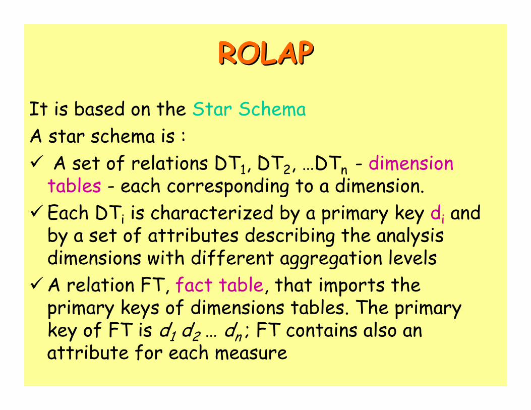
ROLAPROLAP
It is based on the Star SchemaA star schema is :
A set of relations DT1, DT2, …DTn - dimension tables - each corresponding to a dimension. Each DTi is characterized by a primary key di and by a set of attributes describing the analysis dimensions with different aggregation levelsA relation FT, fact table, that imports the primary keys of dimensions tables. The primary key of FT is d1 d2 … dn ; FT contains also an attribute for each measure

Star schema: exampleStar schema: example
SALE
QuantityProfit
shop city stateweekmonth
agent
product
type
categorysupplier
ID_ShopID_WeekID_ProductQuantityProfit
ID_WeekWeekMonth
ID_ProductProductTypeCategorySupplier
ID_ShopShopCityStateAgent
WEEK
PRODUCT
SHOP

Star schema: considerations
• Dimension table keys are surrogates, for space efficiency reasons
• Dimension tables are de-normalized product type category is a transitive dependency
• De-normalization introduces redundancy, but fewer joins to do
• The fact table contains information expressed at different aggregation levels

OLAP queries on Star Schema
select City, Week, Type, sum(Quantity)from Week, Shop, Product, Salewhere Week.ID_Week=Sale.ID_Week and
Shop.ID_Shop=Sale.ID_Shop and Product.ID_Product=Sale.ID_Product andProduct.Category = ‘FoodStuff’
group by City,Week,Type
ID_ShopID_WeekID_ProductQuantityProfit
ID_WeekWeekMonth
ID_ProductProductTypeCategorySupplier
ID_ShopShopCityStateAgent
WEEK
PRODUCT
SHOP
SALE
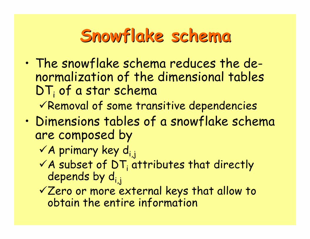
Snowflake schemaSnowflake schema• The snowflake schema reduces the de-
normalization of the dimensional tables DTi of a star schema
Removal of some transitive dependencies • Dimensions tables of a snowflake schema
are composed by A primary key di,jA subset of DTi attributes that directly depends by di,jZero or more external keys that allow to obtain the entire information

Snowflake schemaSnowflake schema• In a snowflake schema
Primary dimension tables: their keys are imported in the fact table Secondary dimension tables

Snowflake schema
ID_ShopID_WeekID_ProductQuantityProfit
ID_WeekWeekMonth
ID_ProductProductID_TypeSupplier
ID_ShopShopID_CityAgent
WEEK
PRODUCT
SHOP
ID_CityCityState
CITY
ID_TypeTypeCategory
TYPE
DT1,1
DT1,2
d1,1
d1,2
External key
SALE
QuantityProfit
shop city stateweekmonth
agent
product
type
categorysupplier

Snowflake schema: considerations
• Reduction of memory space• New surrogate keys• Advantages in the execution of queries
related to attributes contained into fact and primary dimension tables

Normalization & Snowflake schema
• If there exists a cascade of transitive dependencies, attributes depending (transitively or not) on the snowflake attribute are placed in a new relation

OLAP queries on snowflake schema
ID_ShopID_WeekID_ProductQuantityProfit
ID_WeekWeekMonth
ID_ProductProductID_Type
Category
Supplier
ID_ShopShopID_City
State
Agent
WEEK
PRODUCT
SHOP
ID_TypeType
TYPE
ID_CityCity
CITY
select City, Week, Type, sum(Quantity)from Week, Shop, Type, City, Product, Salewhere Week.ID_Week=Sale.ID_Week and
Shop.ID_Shop=Sale.ID_Shop and Shop.ID_City=City.ID_City andProduct.ID_Product=Sale.ID_Product andProduct.ID_Type=Type.ID_Type andProduct.Category = ‘FoodStufs’
group by City,Week, Type

ViewsViews• Aggregation allows to consider concise
(summarized) information• Aggregation computation is very
expensive pre-computation• A view denotes a fact table containing
aggregate data

Views
• A view can be characterized by its aggregation level (pattern)– Primary views: correspond to the primary
aggregation levels– Secondary views: correspond to secondary
aggregation levels (secondary events)

Views (MultiDimensional Lattice)
v1={product,date,shop}
v2={type,date,city}
v3={category,month,city}v4={type,month,region}
v5={trimester,region}
vi <= vj iff vi is lessaggregate than vj, i.e. vj’s data can becomputed from vi’s data
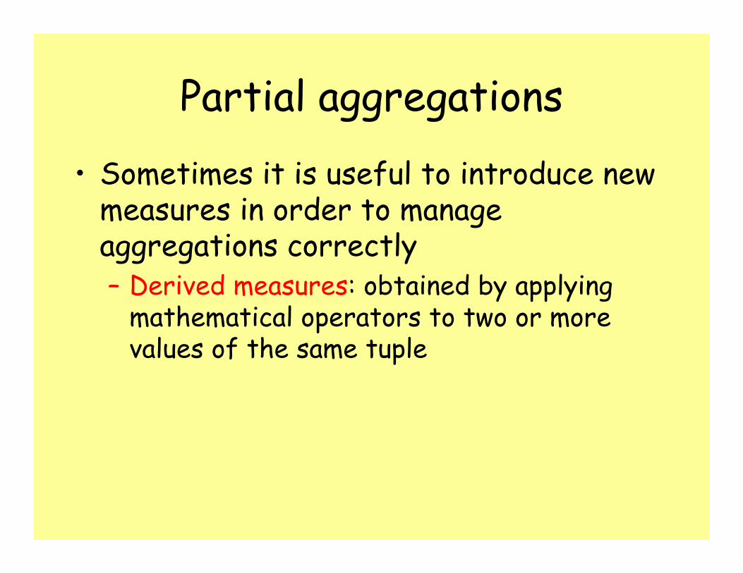
Partial aggregations
• Sometimes it is useful to introduce new measures in order to manage aggregations correctly– Derived measures: obtained by applying
mathematical operators to two or more values of the same tuple

Partial aggregations
The correct solution consists in the aggregation of data
on the primary table
Type Product Quantity PriceT1T1T2
P1P2P3
579
1,001,500,80
Profit5,0010,507,20
Type Quantity PriceT1T2
129
1,250,80
Profit15,007,20
SUM AVG22(total profits)
,70
22,20WeWe cancan’’t just sum up t just sum up profitsprofits asas beforebefore!!!!
Profit=Quantity*Price

Aggregate operators• Distributive operator: allows to
aggregate data starting from partially aggregated data (e.g. sum, max, min)
• Algebraic operator: requires further information to aggregate data (e.g. avg)
• Holistic operator: it is not possible to obtain aggregate data starting from partially aggregate data (e.g. mode, median)
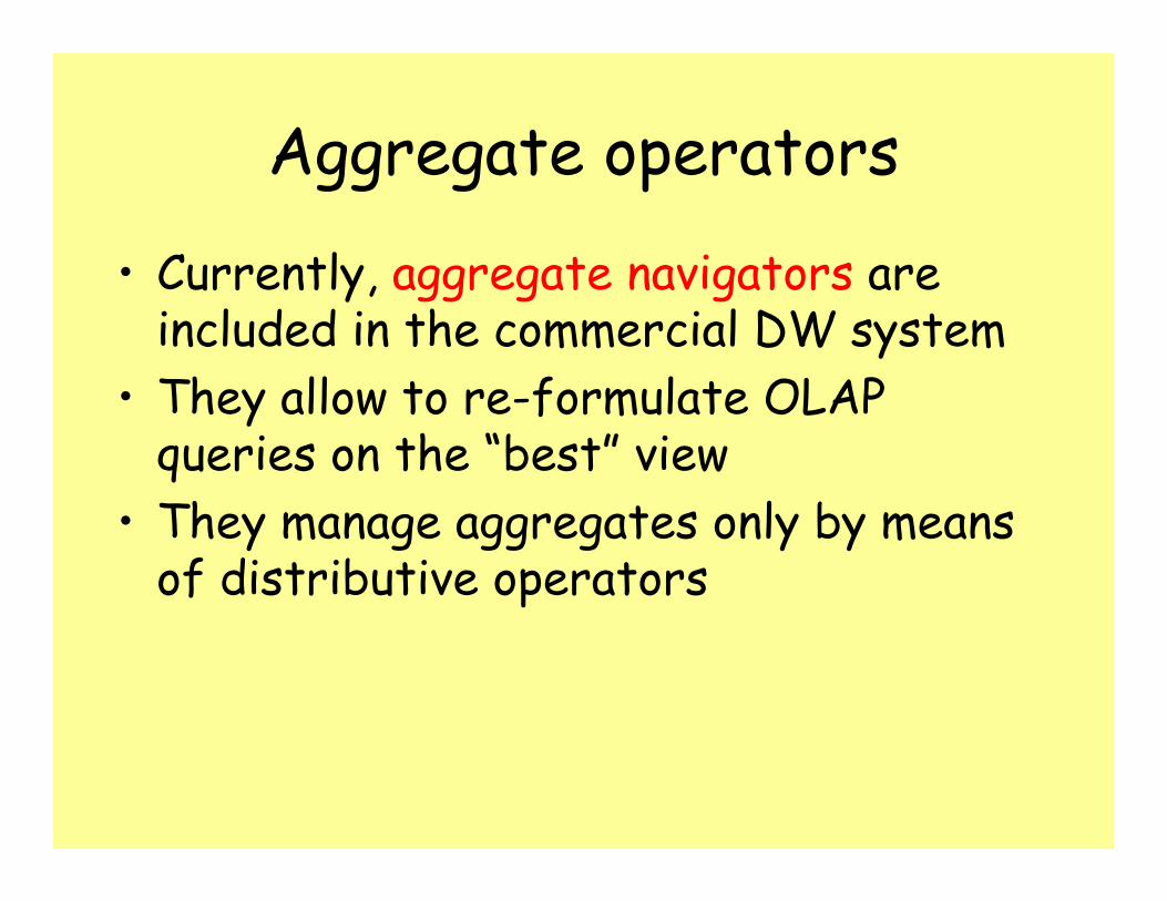
Aggregate operators
• Currently, aggregate navigators are included in the commercial DW system
• They allow to re-formulate OLAP queries on the “best” view
• They manage aggregates only by means of distributive operators

Relational schema and aggregate data
• It is possible to define different variants of the star schema in order to manage aggregate data
• First solution: data of primary and secondary views are stored in the same fact table– NULL values for attributes having
aggregation levels finer than the current one

Aggregate data in aunique fact table
…………………8501700113…150300112…85170111…profitqtyProd_keyDate_keyShop_key
SALE
………………Lazio--3…LazioRoma-2…E.R.BolognaCOOP11…regioncityshopShop_key
SHOP
1° row represents sale values for the single shop, 2° rowrepresents aggregate values for Roma, 3°row representsaggregate values forLazio, etc…

Relational schema and aggregate data
• Second solution: distinct aggregation patterns are stored in distinct fact tables: constellation schema
• Only the dimension of the fact table is optimized, but this is a great improvement already
• Max optimization level: separate fact tables, and also repeated dimension tables for different aggregation levels

Constellation schemaDate_key
Shop_key
QuantityProfit
Unitary priceNr. customers
Date_key
DateMonth
TrimesterYearDay
Week
Shop_key
Date_key
QuantityProfit
Unitary priceNr. customers
Product_key
Shop_key
ShopShop city
Shop regionShop stateManagerdistrict
Product_key
ProductType
CategoryDivision
Marketing groupBrand
Brand city
DATE
SHOP
PRODUCT
v1
v5
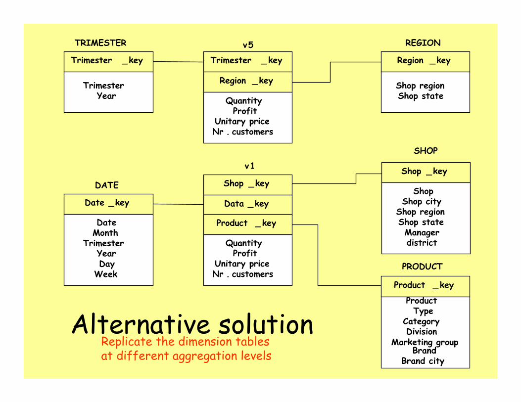
Alternative solution
Trimester _key
Region _key
QuantityProfit
Unitary priceNr . customers
Date _key
DateMonth
TrimesterYearDay
Week
Shop _key
Data _key
QuantityProfit
Unitary priceNr . customers
Product _key
Shop _key
ShopShop city
Shop regionShop stateManagerdistrict
Product _ key
ProductType
CategoryDivision
Marketing groupBrand
Brand city
DATE
SHOP
PRODUCT
v1
v5
Trimester _ key
TrimesterYear
TRIMESTER
Region _key
Shop regionShop state
REGION
Replicate the dimension tablesat different aggregation levels

Snowflake schema for aggregate
data
Date _ key
DateMonth
Trimester _ keyYearDay
Week
DATE
Trimester _ key
Region _ key
QuantityProfit
Unitary priceNr . customers
Shop _ key
Date _ key
QuantityProfit
Unitary priceNr . customers
Product _ key
Shop _ key
ShopShop city
Region _ keyShop stateManagerdistrict
Product _ key
ProductType
CategoryDivision
Marketing groupBrand
Brand city
SHOP
PRODUCT
v1
v5
Trimester _ key
TrimesterYear
TRIMESTER
Region _ key
Shop regionShop state
REGION

Logical design
Logical modelling
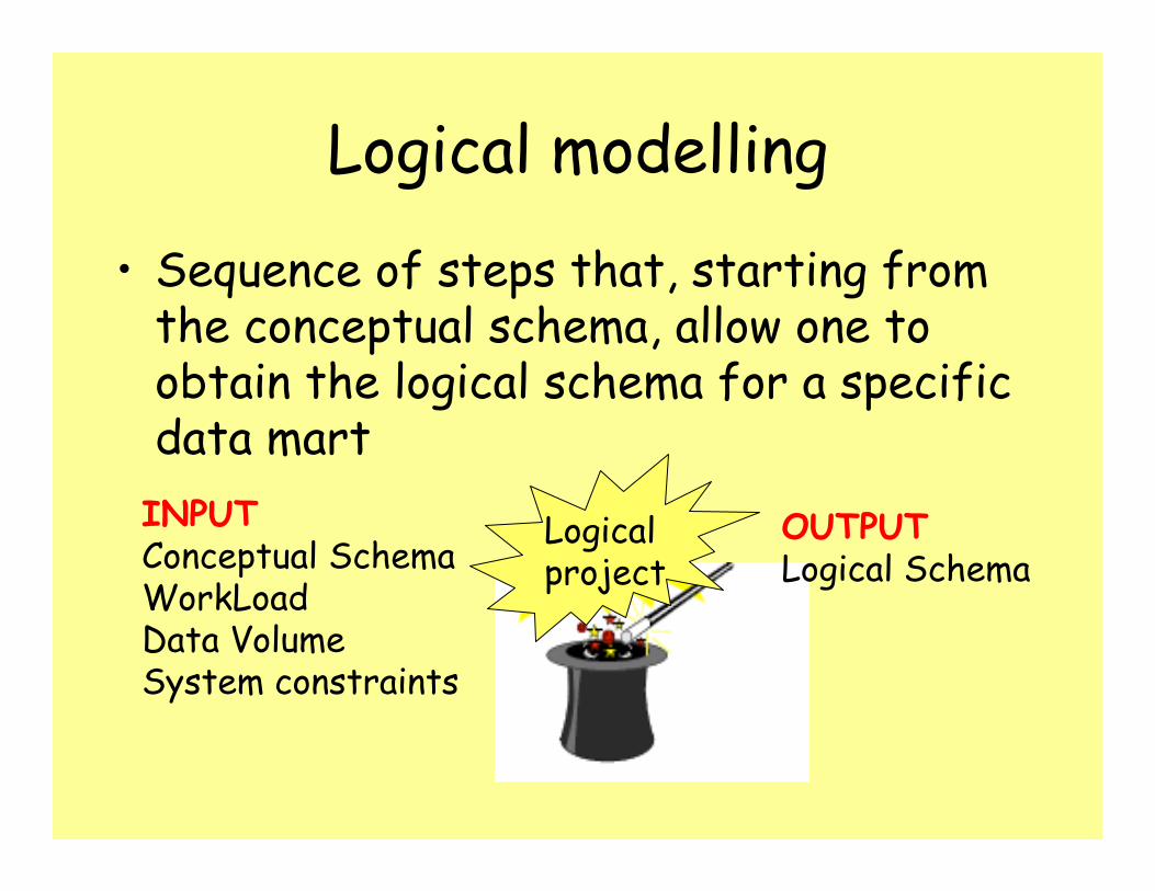
• Sequence of steps that, starting from the conceptual schema, allow one to obtain the logical schema for a specific data mart
Logical project
INPUTConceptual SchemaWorkLoadData VolumeSystem constraints
OUTPUTLogical Schema

Worklad• In OLAP systems, workload is dynamic in
nature and intrinsically extemporaneous– Users’ interests change during time– Number of queries grows when users gain
confidence in the system– OLAP should be able to answer any
(unexpected) request• During requirement collection phase,
deduce it from:– Interviews with users– Standard reports

Worklad• Characterize OLAP operations:
– Based on the required aggregation pattern– Based on the required measures– Based on the selection clauses
• At system run-time, workload can bedesumed from the system log

Data volume• Depends on:
– Number of distinct values for each attribute– Attribute size– Number of events (primary and secondary)
for each fact• Determines:
– Table dimension– Index dimension– Access time
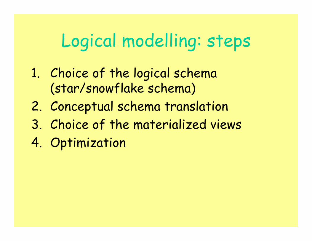
Logical modelling: steps
1. Choice of the logical schema (star/snowflake schema)
2. Conceptual schema translation3. Choice of the materialized views4. Optimization

From fact schema to star schema
• Create a fact table containing measures and descriptive attributes directly connected to the fact
• For each hierarchy, create a dimension table containing all the attributes

Guidelines
• Descriptive attributes (e.g. color)– If it is connected to a dimensional
attribute, it has to be included in the dimension table containing the attribute (see slide n. 13, snowflake example, agent)
– If it is connected to a fact, it has to be directly included in the fact schema
• Optional attributes (e.g. diet)– Introduction of null values or ad-hoc values

Guidelines
• Cross-dimensional attributes (e.g. VAT)– A cross-dimensional attribute b defines an
N:M association between two or more dimensional attributes a1,a2, …, ak
– It requires to create a new table including band having as key the attributes a1,a2, …, ak

Guidelines• Shared hierarchies and convergence
– A shared hierarchy is a hierarchy which refers to different elements of the fact table (e.g. caller number, called number)
– The dimension table should not be duplicated– Two different situations:
• The two hierarchies contain the same attributes, but with different meanings (e.g. phone call caller number, phone call called number)
• The two hierarchies contain the same attributes only for part of the hierarchy trees

Shared hierarchies and convergence
• The two hierarchies contain the same attributes, but with different meanings (e.g. phone call caller number, phone call called number)
N_OF_CALLSDATE_IDCALLED_IDCALLER_IDCALLS
DISTRICT
PH_NUMRUSER_ID
USER

Shared hierarchies and convergence
NUMBER
DATE_ID
ORDER_ID
STOREHOUSE_IDSHIPPINGS
CUSTOMER
ORDER
ORDER_IDORDERS
REGION
CITY_ID
CITIES
CITY_ID
STOREHOUSE
STOREHS_ID
STOREHOUSE
CITY_ID
• The two hierarchies contain the same attributes only for part of the trees. Here we could also decide to replicate the shared portion
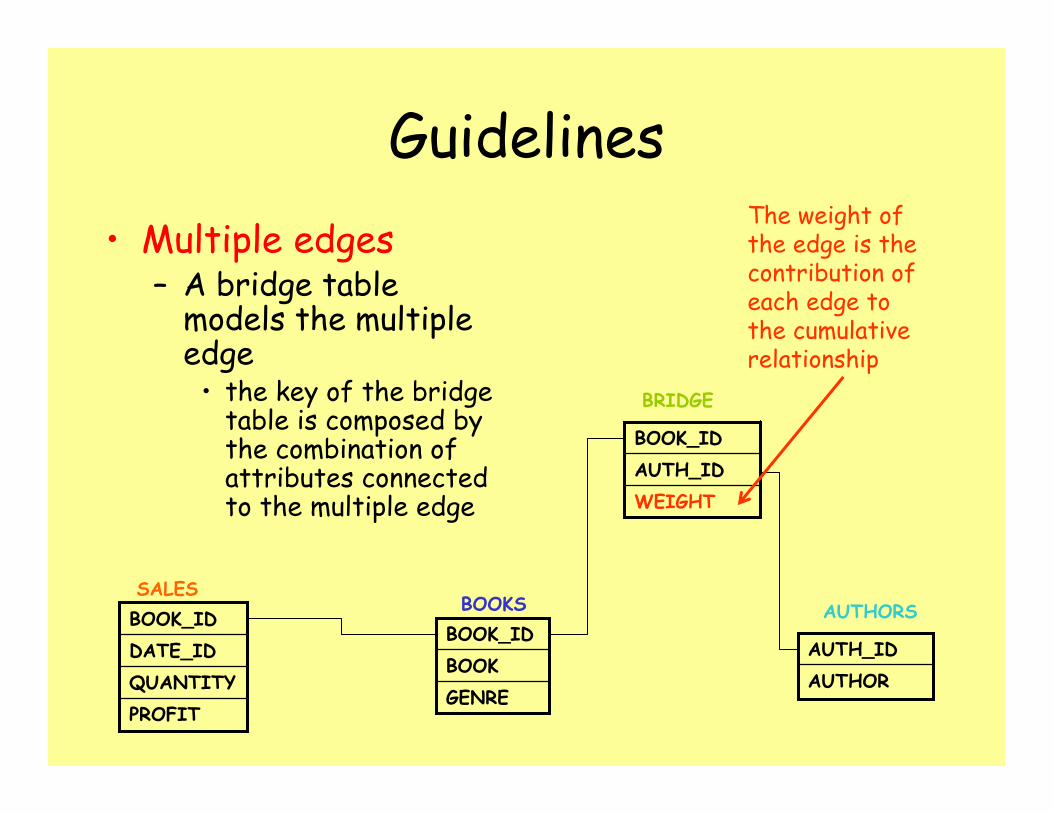
Guidelines• Multiple edges
– A bridge table models the multiple edge
• the key of the bridge table is composed by the combination of attributes connected to the multiple edge
PROFITQUANTITYDATE_IDBOOK_IDSALES
GENREBOOKBOOK_IDBOOKS
AUTHORAUTH_ID
AUTHORS
WEIGHTAUTH_IDBOOK_ID
BRIDGE
The weight of the edge is the contribution of each edge to the cumulative relationship

Guidelines
• Multiple edges: bridge table– Weighed queries take into account the
weight of the edge
Profit for each author
SELECT AUTHORS.Author,SUM(SALES.Profit * BRIDGE.Weight)FROM AUTHORS, BRIDGE, BOOKS, SALESWHERE AUTHORS.Author_id=BRIDGE.Author_idAND BRIDGE.Book_id=BOOKS.Book_idAND BOOKS.Book_id=SALES.Book_idGROUP BY AUTHORS.Author
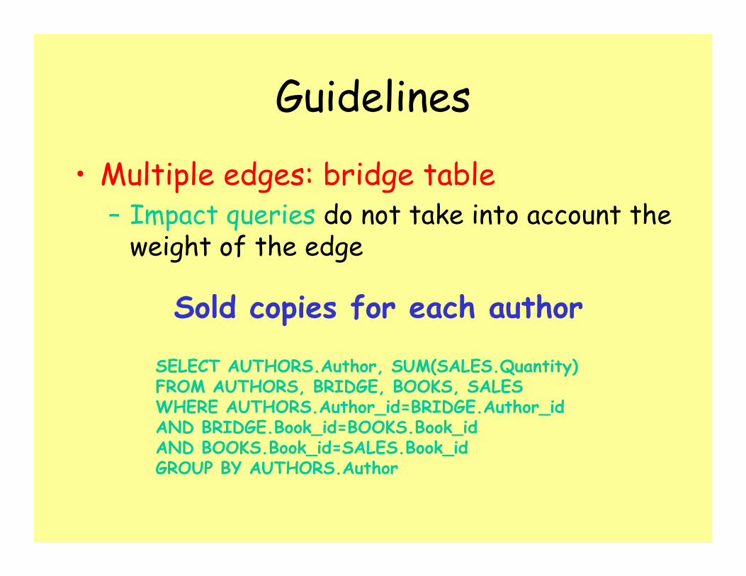
Guidelines
• Multiple edges: bridge table– Impact queries do not take into account the
weight of the edge
Sold copies for each author
SELECT AUTHORS.Author, SUM(SALES.Quantity)FROM AUTHORS, BRIDGE, BOOKS, SALESWHERE AUTHORS.Author_id=BRIDGE.Author_idAND BRIDGE.Book_id=BOOKS.Book_idAND BOOKS.Book_id=SALES.Book_idGROUP BY AUTHORS.Author

If we want to keep the star model
Multiple edges with a star schema: add authors to the fact schema
PROFITQUANTITYDATE_ID
BOOK_ID
SALES
GENREBOOKBOOK_IDBOOKS
AUTHORAUTH_ID
AUTHORSAUTH_ID
Here we don’t need the weight because the fact table records quantity and profit per book and per author
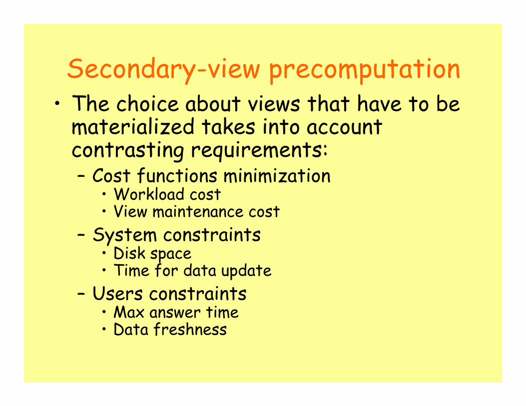
Secondary-view precomputation• The choice about views that have to be
materialized takes into account contrasting requirements:– Cost functions minimization
• Workload cost• View maintenance cost
– System constraints• Disk space• Time for data update
– Users constraints• Max answer time• Data freshness
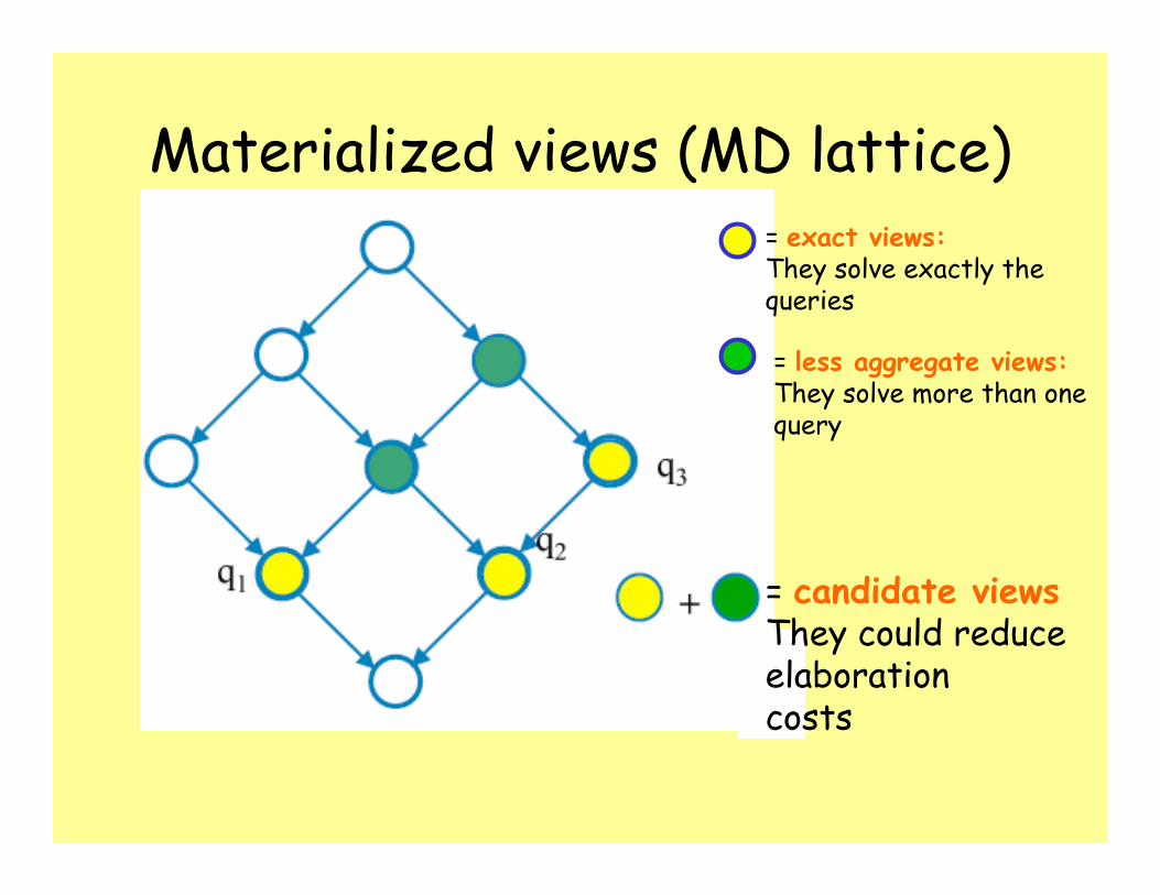
Materialized views (MD lattice)
= candidate viewsThey could reduceelaboration costs
= exact views:They solve exactly the queries
= less aggregate views:They solve more than one query
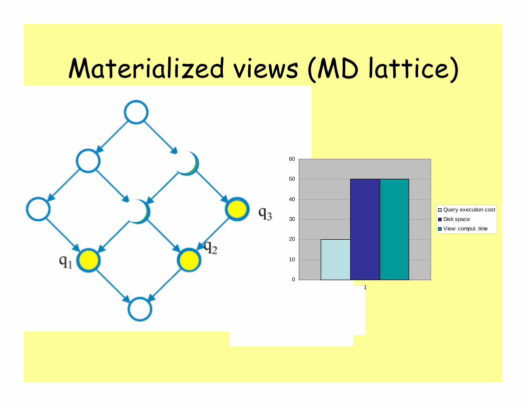
Materialized views (MD lattice)
0
10
20
30
40
50
60
1
Query execution cost
Disk space
View comput. time

Materialized views (MD lattice)
0
10
20
30
40
50
60
1
Query execution cost
Disk space
View comput. time

Materialized views (MD lattice)
0
5
10
15
20
25
30
1
Query execution cost
Disk space
View comput. time

Materialized Views• It is useful to materialize a view when:
– It directly solves a frequent query– It reduce the costs of some queries
• It is not useful to materialize a view when:– Its aggregation pattern is the same as
another materialized view– Its materialization does not reduce the
cost
ReferencesReferences
• M. Golfarelli, S. Rizzi: Data Warehouse: teoria e pratica della progettazioneMcGraw-Hill, 2002.
• Ralph Kimball: The Data Warehouse Toolkit: Practical Techniques for Building Dimensional Data WarehousesJohn Wiley 1996.