Embed Size (px)
Citation preview

NSSDC/WDC-A-R&S 92-05
Data Synthesis and Display
Programs for
Wave Distribution Function Analysis
L. R. O. Storey and K. J. Yeh
June 1992
National Space Science Data Center (Code 630)
NASA/Goddard Space Flight Center
Greenbelt, Maryland 20771, U.S.A.
https://ntrs.nasa.gov/search.jsp?R=19930001612 2018-08-30T05:05:52+00:00Z


Contents
Abstract ................................................
1o
2.
3.
4.
5.
6.
7.
8.
.................................................................................. ° ......... 1
Introduction ............................................................................................................................. 3
Data Reduction ........................................................................................................................ 7
Basic Equation ......................................................................................................................... 9
Data Synthesis ....................................................................................................................... 11
Data Display .......................................................................................................................... 13
Technical Aspects .................................................................................................................... 15
Acknowledgments .................................................................................................................... 17
References ............................................................................................................................... 19
PR_CEO!NG p ,, .-',c iii......_c I_!.._',!_( PJOT FIL_'D


Abstract
At the National Space Science Data Center (NSSDC) software has been written to synthesize and
display artificial data for use in developing the methodology of wave distribution analysis. This
software comprises two separate interactive programs, one for data synthesis and the other for data
display.


1. Introduction
When the fields of natural radio waves are observed and measured by instruments on spacecraft, the
experimenter often wants to know in what directions the waves are traveling. It helps if data from the
wave receivers can be analyzed to yield sky maps showing how the intensity of the waves varies as a
function of direction over the celestial sphere, like the maps that astronomers make.
At low frequencies, however, the sky maps used by space radiophysicists differ from those used by
astronomers. The differences concern, among other things, the definitions of the direction and intensityof a wave.
One difference concerning the direction is simply a matter of convention. Optical and radio astronomers
are accustomed to sky maps in which the properties of the waves are plotted versus direction of
arrival. This is the direction from which the waves are coming, or in other words, the direction of the
line of sight from the observer to the source of the waves. In radiophysics, however, the behavior of
waves is commonly discussed in terms of the direction of propagation, which is the direction in which
the waves are going, i.e., the opposite of the direction of arrival. Hence, radiophysicists use the
direction of propagation as the independent variable for sky mapping.
The other main differences are physical matters. They are due to the presence in space of plasma
permeated by magnetic fields.
At frequencies so low that the plasma affects the waves, the direction of propagation of theirwavefronts, or wave normal direction, is not the same as the direction of propagation of their energy, or
ray direction; the relation between these two directions has been explained by many authors [1-3]. In
making sky maps, radiophysicists prefer to use the wave normal direction because it identifies a wave
unambiguously. This means that for a given wave normal direction there can be only one ray direction,
whereas for a given ray direction there may be two or more, or even, in some special cases, infinitely
many possible wave normal directions.
To specify the direction of the wave normal, a set of right-handed Cartesian axes Oxyz is adopted
with Oz parallel to the local vector B 0 of the Earth's magnetic field, and Ox parallel to the projection
into the plane perpendicular to B 0 of the radius vector from the center of the Earth to the position of
the spacecraft. Then the direction of the wave normal can be specified by the polar angle 0 that it
makes with the z-axis, together with the azimuthal angle _ measured right-handedly around the z-
axis from the x-axis as origin (See Figure 1 below).
Now consider the wave intensity. For waves in free space, it is generally measured by the wave power
per unit area or flux, but this is a vector quantity associated with the ray direction. For a single
coherent wave of constant amplitude, with a unique frequency and a unique wave normal direction,
propagating in a plasma, the wave energy per unit volume or energy density is a more convenient
,.)

measure. Natural radio waves, however, are more often random than coherent, and for random waves
the proper measure is the energy density per unit frequency range and unit solid angle of wave normal
direction. This scalar quantity, considered as a function of frequency and of wave normal direction, is
known as the wave distribution function (WDF).
Z Wavenormal
BoT
x/
/
/
/
/
Y
Figure 1. Coordinate System
A radio sky map is a graphic display of a WDF versus wave normal direction at a fixed frequency.
Customarily, two polar plots are used, one for each hemisphere, with 8 as the radial and _ as the
azimuthal coordinate. Contour lines are used to display the WDF quantitatively. An example is given
in Figure 2 below. The circle forming the outer boundary of the map corresponds to the plane
perpendicular to B 0, here called the equator. The absence of data in a zone centered on the equator is
another effect of the plasma, which at low frequencies forbids propagation at values of e (or of 180 ° - 0
if e > 90 °) larger than a certain value known as the resonance angle.
90. 90.
i O. 180. O.
2"10. 2'_0.
Figure 2. Sky Map of an Experimentally Determined WDF [17]
In the radio sky map of Figure 2 above, it is obvious that the angular resolution is very poor indeed
compared with what optical astronomers achieve. This is due to the difficulty of making directive
observations of waves in space at low frequencies, where the wavelengths are much greater than the
dimensions of any antennas that can be deployed from a spacecraft. With a single spacecraft, the best
one can do is make local measurements of the electric and magnetic field vectors of the waves, then
perform a sophisticated data analysis yielding some degree of "super-resolution." The resulting skymaps are relatively crude, but even so they are useful for scientific purposes.
The methodology for analyzing local measurements of radio wave fields in space to obtain the
corresponding wave distribution functions is known as WDF analysis. General methods of WDF
analysis exist, based on the principle of maximum entropy [4-6]. Some other methods are suited only tospecial cases where the waves are coming from just a few point sources [7,8]. There is scope for
improvement in all of these methods, however, and new ones may be needed [9].
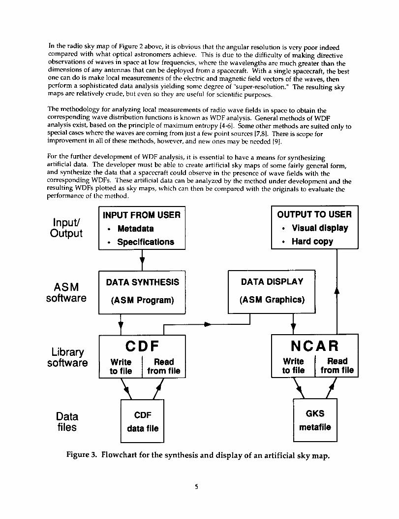
For the further development of WDF analysis, it is essential to have a means for synthesizing
artificial data. The developer must be able to create artificial sky maps of some fairly general form,and synthesize the data that a spacecraft could observe in the presence of wave fields with the
corresponding WDFs. These artificial data can be analyzed by the method under development and theresulting WDFs plotted as sky maps, which can then be compared with the originals to evaluate theperformance of the method.
Input/Output
ASMsoftware
Librarysoftware
Datafiles
INPUT FROM USER
• Metadata
• Specifications
DATA SYNTHESIS
(ASM Program)
t I
CDFWriteto file
Readfrom file
v
OUTPUT TO USER
• Visual display
• Hard copy
DATA DISPLAY
(ASM Graphics)
I
NCAR
Write { Readto file from file
sFigure 3. Flowchart for the synthesis and display of an artificial sky map.

Thepresentreportdescribesasetofsoftwarewrittenforthispurpose.Asshownin theflowchartofFigure 3 above, it consists of two programs: The first, called the Artificial Sky Map (ASM) Program, isfor data synthesis, while the second, called ASM Graphics, is for data display. At the start the user
enters the specifications for an artificial sky map to the ASM Program through an alphanumeric
terminal, while at the finish the ASM Graphics program displays the map on a graphics terminal or a
laser printer; the two terminals can, of course, be the same. Both programs are interactive.
Besides this pair of special-purpose programs, two library software packages are utilized, namely theNSSDC Common Data Format (CDF) scientific data base software [10], and the National Center for
Atmospheric Research (NCAR) Graphics software [11] which uses the standard Graphical Kernel
System (GKS). Data are transferred from the ASM Program to ASM Graphics via a CDF data file, and
from ASM Graphics to the display terminal via a GKS metafile (See Figure 3 above). ASM Graphics
can also accept CDF files created by the WDF analysis programs.
The plan of this report is as follows: Section 2 explains what experimental data are required for WDF
analysis and how they must be reduced beforehand; section 3 presents the basic equation used for
synthesizing artificial data; section 4 describes the, data synthesis program and section 5 the data
display program; section 6 gives some technical details of the software, including how it may be
obtained, while the final sections 7 and 8 contain the acknowledgments and the references, respectively.

2. Data Reduction
When observing natural low-frequency radio waves from a single spacecraft, the best that can be done is
to measure the three components Ex, Ey, and Ez of the electric field vector E together with the three
components H x, Hy, and H z of the magnetic field vector H. Multiplying H by the wave impedance Z 0
of free space turns it into an equivalent electric field, and by this means the entire electromagnetic field
can be represented by a six-component generalized electric field vector _, the components of which are
_1 = Ex _2 = Ey e3 = Ez [
f_4 = zo Hx C5 = ZOmy _6 = Zo Hz
(1)
A set of spacecraft data normally consists of measurements of some or all of the six components of _,
made in a frequency band of width B over a time interval of duration T; here all six components will beassumed to have been measured.
If these data are of good quality and are random, they will be suitable for WDF analysis after some
preliminary processing. The first step is to divide the set into sub-bands of width zlB within which the
spectra of the data are effectively uniform and into sub-intervals of duration AT within which their
statistics are effectively stationary. Then the data from each one of these sub-regions of the frequency-time plane are processed to yield an estimate S for the spectral matrix S of the generalized electric
field, at the center frequency coand center time t of the sub-region concerned. The elements Sij of the
matrix S are the auto-power spectra (if i = j) of the six field components, and the cross-power spectra (if
i _ j) of the 15 pairs of different field components. This processing, which is performed by standard
procedures [12], greatly reduces the amount of data. The init_l data set, consisting of six waveforms of
bandwidth B and duration T, is reduced to a set of estimates Sij for the matrix elements Sij with
relative accuracies of about (AB AT)-1� 2, a total of 36 independent numbers. These reduced data are the
input for the WDF analysis, which should produce as output an estimate for the WDF of the original
wave field at the frequency co and time t.
The artificial data are synthesized at the level of the spectral matrix S, which may be considered as
an ensemble average of the reduced data matrix S, taken over all possible data sets consistent with the
given WDF. Thus, the synthetic data are free from the statistical fluctuations, caused by the non-
infiniteness of AB and AT, that affect real data from spacecraft; they are also free from noise. Whendata from the ASM Program are used for testing new methods of WDF analysis, artificial errors in the
form of both fluctuations and noise are introduced optionally, in a controlled way, by dedicated routines
imbedded in the analysis software.


3. Basic Equation
From specifications entered by the user, the ASM Program tabulates the WDF and computes from it the
corresponding spectral matrix S, the elements of which are related to the WDF by the integral equation
Sij(¢o) = _/2 _ F(co, O,O) aij(o2,O,e)) dry (2)
In the integrand, F is the WDF while the kernels aij are known functions of the angles 0 and 0; for those
directions (8,_) in which propagation is forbidden, the WDF is zero. The integral is taken over the 4K
range of solid angle of which do" = d(cos O)dO is an element [13].
The functional forms of the integration kernels aij are governed by the properties of the ambient plasma
medium. Approximate expressions for them have been published by Storey and Lefeuvre [14]; an error
has been corrected by Lefeuvre et al. [15].
PI:_C_EDtNG PAGF BLA,r,t',_ rJ_.._'._F!L_ED

I 'n'r°_ct'°nI
I .._,_.,oputI
[ WOF°_.,npu,I
I "°Poia i.put
I Input De i St°rageD
I,, _',i°_, I
C Start of Session )
lI IntrOductiOn I
, +_ ore,.,.,.., I
Plot D_a Input I
T
yL_I Display Graphics I
.o !I Session Summary I
C End of Session )
(a) ASM Program (b) ASM Graphics
Figure 4. Operations Performed by the Two Programs
lO

0 Data Synthesis
The ASM Program synthesizes artificial data by the sequence of operations shown in Figure 4a above.
The program has nine major sections, namely Introduction, Metadata Input, WDF Data Input, Map
Data Input, Input Data Storage, Sky Map, Entropy, Spectral Matrix, and Session Summary.
The Introduction acquaints the user with the program. A single paragraph explains its purpose, while
another outlines the interactions that the user should expect.
The Metadata Input section enables the user to enter identifying personal information. The metadata
currently accepted are the user's name, the user's institute or other professional affiliation, and the
date on which the session is taking place. The user is also prompted to enter a name for the artificial
sky map; this name is used as the title for the CDF files in which all the artificial data are stored and
also for the summary text file. The program examines whether any CDF files with this title exist
already and, if so, offers the user the choice of either deleting those files or supplying another name.
The WDF Data Input section serves for entering all the parameters that jointly define the shape of the
model WDF. They comprise firstly some parameters governing the influence of the space plasma and
magnetic field on the waves and secondly the parameters of the wave sources.
In the approximations used here, the influence of the ambient plasma on the waves depends on therelative values of three characteristic frequencies: the electron plasma frequency, which characterizes
the plasma; the electron gyrofrequency, which characterizes the magnetic field; and the frequency ofthe waves themselves. After these parameters have been entered, the program computes from them
the resonance angle Ores. The half-width in 0 of the range of directions around the equator within
which the waves cannot propagate is 90 ° - Ores. The values of 0 at the edges of this forbidden zone are
displayed so that the user can avoid placing any wave sources there.
The model adopted for the WDF provides for wave sources of two kinds: point sources (like stars) and
extended sources (like nebulae). Each point source is characterized by three parameters, namely its
direction angles 0 and 0 and its integrated intensity. For an extended source, the profile of intensity
versus position is approximately Gaussian along any great circle passing through the center of the
source, and the contours of equal intensity are approximately elliptical. The profile would be exactly
Gaussian and the contours exactly elliptical were it not that the program modifies the shape of the
source so that the WDF falls smoothly to zero at the edges of the forbidden zone. Each extended source
is characterized by six parameters, which include the angles 0 and 0 for its center where it is mostintense, and the value of its maximum intensity. The remaining three parameters specify its extension
in terms of the properties of the contour where the intensity is exp(-1/2) -- 0.61 times the maximum
value: They are the half-length of the major axis of the ellipse, the direction of this axis relative tothe local meridian (i.e., the radial line of constant _ passing through the center of the source), and the
axial ratio. Up to ten point sources and ten extended sources can be accommodated in the model.
ll
If the sky map of the WDF is to be tabulated for future visualization, the Map Data Input section
allows the user to enter the specifications for the map grid, which is uniform in both 0 and 0. The user
specifies the number of equal intervals into which the range of each of these variables should be
divided. These are the last of the input data, apart from the user's responses to options.
Next, the Input Data Storage section of the program stores the metadata, the WDF data, and the map
specifications (if any), by writing them to a CDF file. Then, if the user has asked for a sky map to be
tabulated, the Sky Map section computes the WDF at the centers of the map grid cells and stores the
resulting table in the CDF.
Optionally, the Entropy section computes and stores this quantity, which is a nonlinear functional usedin some WDF analysis algorithms (see section 1). Different authors use different expressions for the
entropy, and computations are made for two of these. The relation between them involves the mean
value of the WDF, which is proportional to the total energy density of the wave field, so the mean is
computed and stored as well. This option is offered only if the model WDF contains no point sources,
since the entropy of a point source is infinitely negative.
Again as an option, the Spectral Matrix section computes these artificial data and stores them in the
CDF. The double integrals (2) are evaluated to a nominal accuracy of one part in 10 6 by Romberg
integration [16]. A final option is to have the Session Summary section create a text file containing all
the input data, including the previous options that the user took.
12

o Data Display
The ASM Graphics program, which plots the artificial WDFs as sky maps, has a structure similar to
that of the ASM Program (see Figure 4b above). It has seven major sections: Introduction, Metadata
Input, Data Retrieval, Plot Data Input, Graphics Computation, Graphics Display, and Session
Summary.
The first two sections and the last are very similar to the corresponding ones in the ASM Program,
except that in the Metadata Input section the user is prompted to enter the title of a CDF that already
exists and contains the data for display. The program checks that there is indeed a CDF with this
title in the working directory. If not, it displays a warning and allows the user either to change the
title or to exit from the program and bring the wanted CDF file into this directory.
The Data Retrieval section retrieves the data from the selected CDF using procedures supplied in the
CDF software library. First, it retrieves and displays the metadata that describe the contents of the
file; then it prompts the user either to confirm that this is indeed the wanted file, or to return to the
Metadata Entry section and select a different title. If the user confirms the file, the program then
retrieves its main contents.
Next, in the Plot Data Input section, the user provides some specifications for the sky map. The major
decision is the choice of the hemisphere from which to take the WDF data for plotting; the options are
the Northern Hemisphere data (i.e., those for 0 < 90°), the Southern Hemisphere data (0 > 90°), and
the sum of the data from both hemispheres. After this, the user is asked to accept or reject the printing
of certain enhancements to the map; these include the metadata, the contouring information, a circle at
the resonance angle Ores, and a frame surrounding the polar plot of the WDF.
Graphics Computation is the largest section of the program. It extracts data from the CDF in the light
of the user's options and generates plotting instructions for the map with the help of routines from the
NCAR Graphics library, in particular some contouring routines from a package named CONPACK.
First, the required WDF data are extracted, then processed if necessary, according to the hemisphere
option mentioned above. Then the instructions for the contour plot are generated; this plot concerns onlythe contribution to the WDF from the extended sources. The next set of instructions is for plotting the
positions of the point sources. After this, the program makes the instructions for plotting the polar grid
background for the contours, for printing identifiers such as a serial number and the hemisphere of the
plot, and for printing any enhancements that the user selected. The output from this section is a GKS
graphics metafile with a complete set of instructions for displaying the required sky map on a laser
printer or a terminal screen.
The Graphics Display section reads these instructions from the metafile and sends them to either of the
devices on which the map can be displayed and viewed. Both require the use of a metafile translator,
specifically the one called ctrans in the NCAR Graphics library, to convert data from the metafile to a
format usable by the printer or the terminal. After the map has been displayed, the program asks
13

whethertheuserwishesto plot the data in any of the other possible ways, and if so it returns to the
start of the Plot Data Entry section. Otherwise it continues through the Session Summary section then
terminates the session. An example of an artificial sky map plotted by this program is given in Figure 5below.
Northern Hemisphere
9O
I
120 60
1 50
I
I
I
• !
3O
18O
210
24-0
I
I
I
7 -
I
!
1I
I
l_es
270
300
User, Kevln YehAffiliation, I_SA/GSFC
Date, 9 kugust 1991Hap Nue, try6
CONTOUR FROM 1 TO 10 BY 1
Figure 5. Example of an Artificial Sky Map
14

@ Technical Aspects
Both the ASM Program and the ASM Graphics program are written in Fortran 77. They have a top-
down structure and are amply commented. Their major sections occupy "Level 1" subroutines, which
control all operations dealing with their specific tasks. In each subroutine, all major variables arelisted and defined. The subroutines are self-contained and use no "common" variables. These features
make it easy for the authors and other users to moc:lify the programs if necessary.
The ASM Program exists in two versions: one currently runs on a VAX TM 9410 mainframe under Version
5.4-3 of the VMS TM operating system, using the VAX Fortran V5.5 compiler; the other runs on a Sun TM
4/280 workstation under Unix TM (SunOS TM V4.1.1), using Sun Fortran V1.3.1. The ASM Graphics
program exists only in the latter version. By means of the File Transfer Protocol (FTP), CDFs created bythe VMS version of the ASM Program can be transferred electronically to the Unix system, where the
ASM Graphics program can read them and display their contents. The display uses the Sunview TM
window environment.
Users of VAX/VMS systems may obtain the ASM Program and its descriptive documentation in either
of two ways: via anonymous FTP from the directories [ASM.PROG21] and [ASM.EX2)C] in the
"anonymous" account on ncf.gsfc.nasa.gov (128.183.36.23); and via the NASA Science Internet (NSI,
formerly SPAN) by copying the contents of these two directories, the full names of which areNCF::ANON DIR:[ASM.PROG21] and NCF::ANON_DIR:[ASM.DOC]. A specimen CDF created using
the ASM Program and titled "Example_l" is available, together with the corresponding summary text
file, in the directory NCF::ANON DIR:[ASM.CDF].
Users of Unix systems may obtain the ASM Program, the ASM Graphics program, and the
documentation for both of them by FTP from the "anonymous" account on ncgl.gsfc.nasa.gov(128.183.10.238). The relevant files are in the directories pub/asm/prog31, pub/asm/graph11, and
pub/asm/doc. The specimen CDF "Example_l" and its summary text file are in the directory
pub/asm/cdf. If the ASM Graphics program is run with this CDF as input and the sky map for theNorthern Hemisphere is plotted, the result should be the sky map shown in Figure 5 above.
These two programs use Version 2.1 of the CDF software which is obtainable at no charge from the
NSSDC Coordinated Request and User Support Office. They also use Version 3.01 of the NCAR
Graphics software, and this may be obtained from the User Services Section of the Scientific Computing
Division at the National Center for Atmospheric Research, in Boulder, Colorado.
15


e Acknowledgments
The authors thank J. Love for help with CDF and Fortran, J. Williams for help with NCAR Graphics
and Unix, and A. Sawada for testing the ASM Program and suggesting improvements. They also thank
F. Lefeuvre for permission to reproduce Figure 2 from the Journal of Geophysical Research [17].
This report was written while the first author held a National Research Council Senior Research
Associateship at NASA Goddard Space Flight Center (GSFC). The second author benefitted from a
grant under the Visiting Student Enrichment Program sponsored by the GSFC Space Data and
Computing Division.
The following are registered trademarks: VAX, VMS (Digital Equipment Corporation); Sun, SunOS,
Sunview (Sun Microsystems Inc.); Unix (AT&T).
PRECEDING PAGE BLANK NOT FILMED17


Be References
1. T.H. Stix, The Theory of Plasma Waves (McGraw-Hill, New York, 1962), p. 45.
2. K.G. Budden, The Propagation of Radio Waves (Cambridge University Press, Cambridge,
England, 1985), p. 103.
3. H.G. Booker, Cold Plasma Waves (Martinus Nijhoff, Dordrecht, 1984), p. 67.
4. F. Lefeuvre and C. Delannoy, Ann. Tdldcomm., 34, 204 (1979).
5. F. Lefeuvre, M. Parrot, and C. Delannoy, J. Geophys. Res., 86, 2359 (1981).
6. C. Delannoy and F. Lefeuvre, Comput. Phys. Comm., 40, 389 (1986).
7. L.J. Buchalet and F. Lefeuvre, J. Geophys. Res., 86, 2377 (1981).
8. M. Hayakawa, F. Lefeuvre, and J. L. Rauch, Trans. IEICE, E-73, 942 (1990).
9. L.R.O. Storey, "Radio sky mapping from satellites at very low frequencies," in Environmental
and Space Electromagnetics, edited by H. Kikuchi (Springer-Verlag, Tokyo, 1991), p. 310.
10. NSSDC, NSSDC CDF User's Guide, Version 2.1, Technical notes NSSDC/WDC-A-R&S 91-30 (for
Unix systems) and 91-31 (for VMS systems) (National Space Science Data Center, Greenbelt,1991).
11. F. Clare and D. Kennison, NCAR Graphics Guide to New Utilities, Version 3.00, Technical note
NCAR/TN-341+STR (National Center for Atmospheric Research, Boulder, 1989).
12. F. Lefeuvre and L. R. O. Storey (Centre de Recherches en Physique de rEnvironnement, Orl6ans),
Technical note CRPE/41 (1977).
13. L.R.O. Storey and F. Lefeuvre, Geophys. J. R. Astron. Soc., 56, 255 (1979).
14. L.R.O. Storey and F. Lefeuvre, Geophys. J. R. Astron. Soc., 62, 173 (1980).
15. F. Lefeuvre, Y. Marouan, M. Parrot, and J. L. Rauch, Ann. Geophys., 4A, 451 (1986).
16. W.H. Press, B. P. Flannery, S. A. Teukolsky, and W. T. Vetterling, Numerical Recipes
(FORTRAN Version) (Cambridge University Press, Cambridge, England, 1989), p. 114.
17. F. Lefeuvre and R. A. Helliwell, J. Geophys. Res., 90, 6419 (1985).
PRECEDING i_AGE BLANK NOT FILMED
19