1

GSA Data Repository Item 2019234 Collins, B.D. and Reid, M.E., 2019, Enhanced landslide mobility by basal liquefaction: The 2014 State Route 530 (Oso), Washington, landslide: GSA Bulletin, https://doi.org/10.1130/B35146.1.

DATA REPOSITORY

Data Repository File DR1. Geotechnical testing, volumetric analysis, and liquefaction analysis methods (single Adobe .pdf file contained herein with four sections of text, tables, and figures)

Appendix S1: Geotechnical laboratory testing program (includes Figures S1, S2, S3, Tables S1, S2, S3)

Appendix S2: Methodology for calculating landslide volumes (includes Figure S4, Table S4)

Appendix S3: Methodology for coupled poroelastic model of alluvium (includes Figure S5, Table S5)

Appendix S4: Methodology for cyclic shearing liquefaction evaluation (includes Table S6)

Data Repository File DR2. Mapping and soil geotechnical data (Microsoft Excel .xlsx format as a separate file with five individual sheets)

Data Sheet S1: Geologic mapping data

Data Sheet S2: Sand boil and slosh pit mapping data

Data Sheet S3: Tree height mapping data

Data Sheet S4: Soil grain size distribution data

Data Sheet S5: Soil triaxial test data

2

APPENDIX S1. GEOTECHNICAL LABORATORY TESTING PROGRAM

We provide details of the geotechnical testing program performed on soils sampled at the Oso

landslide for completeness and also as an archive for some of the ephemeral data collected

during our geologic mapping campaign. Sample locations are show in Figure S1. All testing was

performed in the University of California, Berkeley geotechnical engineering laboratory with the

exception of some index testing performed by a commercial laboratory (Cooper Testing Labs,

Palo Alto, California).

Soil characterization testing on field samples included grain-size distribution (ASTM D422-63,

2007), Atterberg limits (ASTM D4318-10e1, 2010), specific gravity (ASTM D854-14, 2014), and

USCS soil characterization (ASTM D2487-11, 2011). On undisturbed samples that could be

collected with hand-pushed brass cylinders, we performed bulk and dry density (ASTM D7263-

09, 2009) and water content (ASTM D2216-10, 2010) testing. Relevant associated parameters

(i.e., D50, Cu, and Cc for grain-size curve data, and void ratio for density and specific gravity

measurements) are provided in Table S1 for debris-flow and liquefied-pool sediment deposits,

and Table S2 for sand boils as well as buried and surface alluvium from the banks of the North

Fork Stillaguamish River. Grain-size distribution data for the curves presented in Figure 14 are

provided in Data Sheet S4 (Data Repository File DR2).

We performed geotechnical triaxial testing on North Fork Stillaguamish River alluvium samples

collected from both an unburied river sand bar immediately upstream of the slide (i.e.,

“surface” samples, Fig. S2) and also from the alluvium buried by the overriding landslide (i.e.,

“buried” samples). We collected the buried alluvium from 8-m-tall cut-bank exposures along

both the north and south sides of the river during field work in September 2014 (Fig. 12); these

3

exposures were subsequently buried by ongoing erosion of the river banks. We collected

samples using hand-pushed, 6.18 cm (2.4-inch) diameter and 15.24 cm (6-inch) tall, thin-walled

brass tubes that we subsequently hand-excavated from the ground (Fig. S2). We determined

field density based on the mass of soil in each tube divided by the volume of the tube. In some

cases, in-situ soil resistance required us to use a small hammer and end cap to further push the

tubes and collect a full sample height. This likely resulted in some minor densification of the

samples, but was subsequently remedied by our laboratory sample preparation method (see

below).

We present data for 6 tests performed using a strain-controlled triaxial device on samples of

surface alluvium collected in July 2016. These samples represent typical alluvium in the North

Fork Stillaguamish River. Whereas we performed some additional tests on buried and

undisturbed (tube-sampled and subsequently extruded) samples under both stress- and strain-

controlled loading (primarily for obtaining generalized elastic deformation parameters for the

Biot modeling – see Appendix S3), we found that sample density in some sample tubes

increased significantly due to post-sampling soil transport and extrusion. For example, upon

opening each sample in the laboratory, several millimeters of settlement were observed in

most tubes with a thin layer of water at the sample top. Because the original (loose) density of

the samples could not be achieved through the extrusion process, we chose to prepare most

samples (including all results presented in Fig. 16) using the moist-tamping method (e.g., Mulilis

et al., 1977). The moist-tamping method has been shown to result in relatively homogeneous

samples that behave similarly (e.g., in liquefaction tests – see Mulilis et al., 1977) to other

methods (i.e., wet pluviation) that might more correctly replicate the natural fabric of alluvium

4

deposits but which can lead to difficulties in controlling the initial sample density (e.g., Amini

and Qi, 2000). The six tests presented here (see Fig. 16) were conducted on reconstituted

moist-tamped samples using six layers per sample to achieve representative field density (and

thus initial void ratio) conditions. For the two “All layers” tests (Fig. 16), the samples were first

extruded from their field sample brass tubes, split longitudinally in half, and separated into six

layers. We performed soil characterization on each layer (Fig. S3), and then subsequently

moist-tamped the soil into the identical layer order of the previously extruded sample. For

“Layer 2” and “Layer 3” tests, we sieved bulk samples of the identical surface alluvium as from

the “All layers” samples, and prepared full-height samples representative of the grain size

distribution of the individual layers from the “All layers” samples (Layer 2 or Layer 3). These

samples were also prepared in six layers, but with each layer identical to all other layers within

each sample.

For all tests, we aimed for relative densities (Dr) on the order of 30 to 50% (Table S3). These

values were determined to be representative of the surface alluvium based on measurements

on field brass-tube samples. Relative density provides a more consistent comparison for soils of

varying grain size composition (e.g., such as for the Layer 2 and Layer 3 soils) compared to void

ratio or dry density (Terzaghi et al., 1996). To calculate relative density, we performed

maximum and minimum density tests on each test soil (All layers, Layer 2, and Layer 3) using

the Japanese standard JIS A 1224:2000 (Test Method for Minimum and Maximum Densities of

Sands, translated to English by Y. Hosono; JIS, 2000). Sample dry densities ranged from 1.468 to

1.600 g/cm3 with equivalent void ratios of 0.72 to 0.87 (Table S3). The void ratio of naturally

deposited sands typically ranges from 0.5 to 1.0 (Cubrinovski and Ishihara, 2002); our

5

reconstituted samples therefore represent typical field conditions, while still achieving the

target relative density range.

Following moist-tamping, we wet the prepared samples using the vacuum consolidation

method (e.g., Lade, 2016) by using a small vacuum gradient (~15 kPa) for high consolidation

stress (p’0 = 100 kPa) samples or a small gravity gradient (~5 kPa) for low consolidation stress

samples (p’0 = 20 kPa). After moving a sample to the triaxial testing frame, we used the back-

pressure saturation method (e.g., Lade, 2016) to achieve saturation with B-values of greater

than 0.95. For the six tests presented herein, we used a strain-controlled loading platform

(moving at 1.5 mm/min = 1% axial strain per minute) under undrained conditions to induce

increasing vertical stresses on the sample and measured cell pressure (σr), pore pressure (μ),

axial load (converted to stress, σa), and vertical soil displacement (axial strain) at a data

collection rate of 5 Hz. We conducted all tests to greater than 15% axial strain to ensure that

critical-state conditions were reached and post-processed all data using standard methods (e.g.,

Lade, 2016) with corrections made for load rod uplift, membrane stiffness, and sample cross-

sectional area using a cylindrical area correction. The data presented in Fig. 16 (deviator stress

q = σa – σr and mean effective stress p’ = (σ’a+ 2σ’r)/3) are products from calculations on these

data (note that effective stress, σ’ = σ – μ). The p’-q triaxial data for the six tests presented

here are provided in Data Sheet S5 in the Data Repository.

The “All layers” tests provided sufficient information to obtain an estimate of the critical state

line (CSL, Figure 16A) (e.g., Wood, 1991; Jefferies and Been, 2015). However, a clear critical

state line for the Layer 3 soil could not be defined because the two tests for this soil were

conducted at nearly the same void ratio. A critical state line for the Layer 2 soil could not be

6

obtained because both tests fully liquefied, thereby indicating that the CSL is somewhere

“below” (in void ratio vs. mean effective stress space, p’) the data for these tests. Finally, we

note that the values of void ratio from our testing (0.72-0.87 with corresponding porosity, n =

0.42-0.47; Table S3) are greater, and thus more likely to contract, compared to those used by

Iverson et al. (2015) (i.e., n = 0.36-0.38) for the Oso landslide mass in their modeling of the

landslide’s mobility. This further emphasizes the role of contractive soil behavior, albeit in the

underlying alluvium, in enhancing landslide mobility.

7

TABLE S1. SOIL CHARACTERIZATION PARAMETERS FOR DEBRIS-FLOW AND LIQUEFIED-POOL SEDIMENT DEPOSITS

Material Sample ID#

Field density (g/cm3)

Gravi-metric water

content (%)

Specific gravity (g/cm3)

Void ratio

Grain size characteristics Atterberg Limits LL/PI (%)

Soil classifi-cation

(USCS)*

D50 (mm)

Cu Cc fines (%)

Debris flow

BDC-04112014-1 N.A.† 78.1 N.D.§ N.A. 0.036 14.7 2.5 80.0 50/11 ML

BDC-04132014-1/2/3 1.908 34.8 2.755 0.90 0.110 3.9 0.6 41.3 np# SM

BDC-04132014-4/5/6 1.888 26.6 2.731 0.87 0.140 57.1 0.7 22.6 21/np SM

KS14OS-7 N.A. N.D. 2.767 N.A. 0.104 144.2 1.6 44.3 28/7 SC-SM

KS14OS-25 2.182 15.1 2.717 0.44 0.350 25.0 2.9 17.4 17/np SM

KS14OS-31 N.A. N.D. 2.760 N.A. 0.168 157.5 4.1 36.7 23/4 SC-SM

KS14OS-34 1.918 22.1 2.763 0.77 0.140 153.3 3.0 40.0 23/10 SC

KS14OS-36 1.839 22.2 2.749 0.83 0.157 56.2 3.8 34.3 16/np SM

JAC1-041014 N.A. N.D. 2.751 N.A. 0.038 49.8 1.2 62.4 33/9 ML

JAC2-041014 N.A. N.D. 2.762 N.A. 0.154 23.6 3.8 29.8 19/np SM

Liquefied-pool sediments

KS14OS-13 2.015 25.3 2.768 0.72 0.299 2.4 1.0 2.7 np SP

KS14OS-43 1.904 22.9 2.774 0.79 0.503- 2.9 1.0 3.5 np SP

*Unified Soil Classification System (USCS) soil abbreviations are: “ML” = low plasticity silt, “SM” = silty sand, “SC” = clayey sand, “SP” = poorly graded sand.

†N.A. = not applicable (e.g., due to bulk sample or drying prior to testing). §N.D. = not determined. #np = non-plastic; liquid and/or plastic limit Atterberg test not able to be performed.

8

TABLE S2. SOIL CHARACTERIZATION PARAMETERS FOR SAND BOILS AND ALLUVIUM

Material Sample ID#

Dry density (g/cm3)

Specific gravity (g/cm3)

Void ratio

Grain size characteristics Atterberg Limits LL/PI (%)

Soil classifi-cation

(USCS)*

D50 (mm)

Cu Cc fines (%)

Sand boil

SB1 N.A.† N.D.§ N.A. 0.215 4.7 0.9 13.9 np# SM

SB3 N.A. N.D. N.A. 0.137 44.0 4.3 35.1 np SM

KS14OS-14 N.A. N.D. N.A. 0.093 3.4 1.0 39.1 np SM

KS14OS-19 N.A. N.D. N.A. 0.190 2.9 1.4 10.2 np SP-SM

KS14OS-40 N.A. N.D. N.A. 0.470 9.0 1.9 10.3 np SW-SM

BDC-04132014-7 N.A. N.D. N.A. 0.280 3.1 1.0 3.8 np SP

BDC-09242015-1 N.A. N.D. N.A. 0.134 4.0 1.3 21.1 np SM

BDC-09242015-11 N.A. N.D. N.A. 0.137 3.2 1.1 19.5 np SM

Alluvium – buried**

BDC-09172014-1 N.A. 2.752 N.A. 0.460 2.6 1.1 1.9 np SP

BDC-09182014-1/2 1.537 2.779 0.81 0.170 10.2 3.3 22.8 np SM

BDC-09182014-4/5 1.427 2.781 0.95 0.150 60.0 3.0 35.0 np SW-SC

BDC-09182014-7/8/9 1.494 2.764 0.85 0.220 3.8 1.4 17.0 np SP-SM

Alluvium – surface**

BDC-09232015-1/3/4 1.426 N.D. 0.94†† 0.436 3.8 1.3 4.0 np SP

BDC-09232015-5/8 1.383 N.D. 1.00†† 0.430 2.9 1.3 4.4 np SP

BDC-07122016-1/2/19 1.502 2.751 0.83 0.842 9.3 1.2 5.9 np SW

BDC-07122016-7/8/20 1.524 2.776 0.82 0.529 4.8 1.0 6.3 np SP

*Unified Soil Classification System (USCS) soil abbreviations are: “SM” = silty sand, “SC” = clayey sand, “SP” = poorly graded sand, “SW” = well graded sand.

†N.A. = not applicable (e.g., due to bulk sample or drying prior to testing).

9

§N.D. = not determined. #np = non-plastic; liquid and/or plastic limit Atterberg test not able to be performed. **Although the average dry density of the buried alluvium (1.486 g/cm3; Fig. 12) is greater than the surface alluvium

(1.459 g/cm3) and suggests densification by the overriding landslide, the difference is not statistically significant (i.e., the data fails a two sample t-Test) due, in part, to the small number of samples (nburied = 3 and nsurface = 4).

††Void ratio based on specific gravity from other tests of similar samples.

10

TABLE S3. GEOTECHNICAL TRIAXIAL TEST SAMPLE PREPARATION DATA FOR NORTH FORK STILLAGUAMISH RIVER ALLUVIUM

Confining stress (kPa)

Relative density*

(%) Void ratio

All layers soil

20 30 0.83

100 36 0.81

Layer 2 soil

20 45 0.72

100 42 0.73

Layer 3 soil

20 37 0.87

100 41 0.86

*Relative density was determined based on maximum and minimum void ratios computed for each soil.

11

Figure S1. Map showing location of samples used in geotechnical characterization and triaxial

testing. Colors denote type of sediment sample. NFSR—North Fork Stillaguamish River.

12

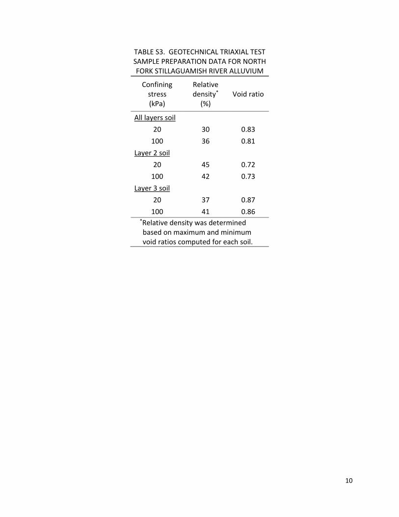
Figure S2. Soil-sampling method used to collect surface alluvium samples for geotechnical

triaxial testing. The sample location is a newly formed river sand bar on the upstream end of

the 2014 Oso landslide and thus representative of the surficial alluvium present in the

floodplain prior to being overridden by the landslide.

13

Figure S3. Soil grain-size distribution curves of individual soil layers of the alluvial sediment

used for geotechnical triaxial testing to investigate the susceptibility to liquefaction failure of

alluvium present in the North Fork Stillaguamish River valley bottom. Sediment layers are

divided evenly but account for stratigraphic divisions observed in the soil texture. Soil layers

used for triaxial testing are shown as “Layer 2”, “Layer 3”, and “All layers”.

14

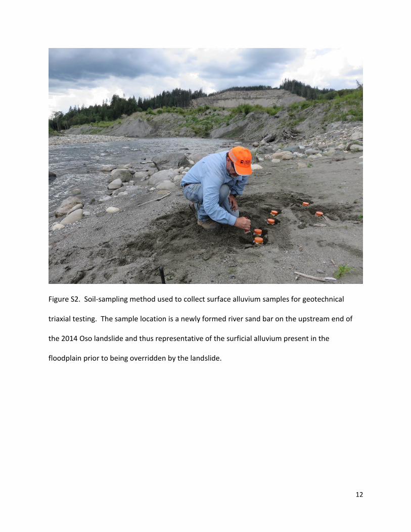
APPENDIX S2. METHODOLOGY FOR CALCULATING LANDSLIDE VOLUMES

Our calculation of landslide source and deposit volumes relied on the construction of high

resolution ground and failure surfaces using available lidar data (preslide July 2013 data

available from the Puget Sound Lidar Consortium, http://pugetsoundlidar.ess.washington.edu/

and postslide, 26 March 2014 and 6 April 2014 data provided by WSDOT,

http://www.wsdot.wa.gov/mapsdata/Photogrammetry/3DTL.htm). Whereas ground surfaces

were relatively straightforward to construct, defining the topography of the failure surfaces at

depth required incorporating several sources of disparate subsurface information. These

included: (1) lidar points of the exposed head and lateral scarps, (2) failure surface borehole

intersections, (3) a curvilinear cross-section line connecting the boreholes to the headscarp, (4)

field mapping evidence of areas outcropping near the failure surface, and (5) the mapped,

three-dimensional boundary of the landslide mass.

The geotechnical drilling investigation conducted following the landslide (Badger, 2016)

revealed a failure-surface depth that emplaced outwash and presumed headscarp colluvium

infilling (Qc; Fig. 4, Fig. 8) unconformably over deeper glaciolacustrine silt and clay (Qglv) just

below the Whitman headscarp at an elevation of 122-124 m (WSDOT borehole EB-04si-15; Fig.

8), and approximately 80 m below the (preslide) conformable Qgov-Qglv contact. Further

confirmation of the failure surface beneath the Whitman mass was provided by field

observations where an internal slice of the Whitman component exposed a flat area (Fan Lake,

Fig. 3) that, based on geometrical inferences connecting the WSDOT boreholes and the

overriding surface exposed at the new alignment of the North Fork Stillaguamish River (see Fig.

12), is located close to the failure surface. An additional borehole on the upper east side of the

15

Whitman component (WSDOT borehole – EB-05si-15) also identifies the Whitman failure

surface with displaced advance outwash (Qgov) overlying glaciolacustrine deposits (Qglv) at 135

m elevation, which is approximately 50 m below the expected (pre-landslide) conformable

contact in that location. Note that borehole EB-05si-15 is 200 m off-section in Fig. 8 (see also

Fig. 4) and therefore the stratigraphy does not match precisely the elevations shown in the

section. We also used several other boreholes (H-15vwp-15, EB-07si-15, and EB-09si-15) in the

failure surface construction that provide evidence of the basal shear plane.

Using this borehole information, along with the other topographic information, we created a

failure surface underlying the source area and thereby calculated an estimate (lower bound) for

the source area volume (7,934,000 m3). We then created a slightly more complex 3D failure

surface geometry by assuming that the off-axis boreholes on the east scarp (WSDOT boreholes

EB-05si-15 and EB07si-15; Fig. 4) could be mirrored and translated to similar locations along the

western scarp. Similarly, we translated the curvilinear longitudinal axis cross-section line of the

failure surface both to the east and west to further refine the geometry. Construction of this

failure surface enabled an additional (upper bound) volume estimate of the Oso landslide

source (10,079,000 m3). We report the average of these two estimates for the final estimated

volume of the landslide source area (Table 1).

We similarly calculated the presumed source volumes for the two other components (Hazel

slide and Paleo slide) through reconstruction and projection of visible pre-Oso landslide scarps

to the depth of the reconstructed Oso landslide failure surface. For the Paleo source volume,

we constructed several possible failure surfaces that intersected the existing pre-2014

geometry of the Paleo bench and identified the most plausible surface based on the measured

16

deposit volumes. We found that any Paleo source failure surface steeper than we present (Fig.

8) resulted in an unreasonably low (i.e., near or below zero) volumetric expansion ratio

between source and deposit. Similarly, we found that any failure surface that did not include

some part of the Paleo source resulted in an unreasonably large (i.e., on the order of 50%)

expansion ratio. Thus, our Hazel-Paleo source failure surface is constrained by these

calculations and analyses.

We determined the volumes of all components of the 2014 landslide (Whitman, Paleo, Hazel,

and debris flow) by direct comparison of the triangulated irregular networks (TINs) of the

constructed surfaces. For source volumes, we compared the preslide surface to the failure

surface, and for deposit volumes, we compared the postslide surface to the preslide surface.

Most volumes were calculated as described in the “Methods” section. To determine the

volume of the debris-flow part of the landslide deposit, we measured the area covered by

debris-flow veneer and multiplied this by the average flow depth measured on the back sides of

still-standing trees in the distal debris field. Here we assume that the average flow depth is

representative of the debris-flow deposit thickness. Flow depth measurements on standing

trees were made in the weeks and months following the landslide (Fig. 11A) and consisted of

three observations: the front-side scour height, the front-side (maximum) splash height, and

the back-side flow depth (Table S4, Fig. S4). In most cases, measurements were made manually

using a measuring tape and data were recorded to the nearest decimeter. In a few cases

(splash heights greater than 3 m), measurements were estimated by referencing a measuring

tape located at the lower section of the tree. Although the front-side scour and splash heights

were always greater than the back-side flow depth, dynamic runup and idiosyncrasies in the

17

mechanics of flow (e.g., scour heights from dislodged tree limbs dragging onto in-place trees)

precluded using these (front-side) measurements to estimate flow depth. Thus, the back-side

flow depth provided the most realistic estimate of overall debris flow thickness at the far distal

ends of the deposit. We calculated separate average flow depths in the west and east lobes

based on six and seven back-side flow depth tree measurements, respectively (Table S4, Fig.

S4).

To calculate the volume of water in the North Fork Stillaguamish River presumably entrained

during the initial motion of the landslide across the valley, we computed a river entrainment

area of 97,000 m2 from widths of the river and landslide, and an average river depth of 0.8 m

based on stream gage data comparison between the Arlington gage (#12167000), located

approximately 23 km downstream of the landslide which was operating at the time of the

landslide, and the C-Post Road Bridge gage (#12166185), located just upstream of the landslide

which was installed shortly after the landslide (Magirl et al., 2015 and on-line data available

from https://waterdata.usgs.gov/wa/nwis/sw). For this analysis, we correlated the river depth

at the time of landsliding (when only the Arlington gage was operating) to the ratio of the river

depth at other times of year for which both gages were in operation. For volume total

calculations, we assume that the resultant volume of entrained North Fork Stillaguamish River

water (78,000 m3) was integrated into the impacting slide materials (i.e., Hazel landslide

source). Although there was some water visible in standing pools at the distal end of the 2014

landslide deposit immediately after the event, we believe the majority of water was

incorporated into the debris-flow deposit and is therefore captured by this volume.

18

Given the high quality and resolution of the lidar data sets (our bare earth models of ground

surfaces were each composed of approximately 2 million points with a 2-meter point spacing),

we have high confidence (<1% error) in the volumes calculated for the landslide deposit areas

with the exception of the debris-flow and the Whitman component. For the debris-flow

volume, our estimate may be between one half to twice as large as the actual deposit volume,

but cannot be constrained any further due to the difficulty in distinguishing the component of

debris-flow veneer (especially reflected backwash) from the underlying Hazel component

deposit. The assumptions made for the construction of the three-dimensional failure surface

beneath the Whitman source area result in somewhat larger error (±12 to 16%) for the

Whitman source and deposit volumes, respectively. Overall, our volume calculations resulted

in a 6% difference (i.e., landslide volume expansion ratio) between total source to deposit

volume (Table 1) which appears reasonable given that the majority of interparticle motion was

confined to the shear plane and that the lidar data was of sufficiently high resolution to account

for most extensional voids between hummocks.

19

TABLE S4. DEBRIS FLOW DEPTH MEASUREMENTS FROM TREE ON-LAP OBSERVATIONS

Observation #

Easting* (m)

Northing* (m)

Flowline distance†

(m)

Front side

scour height

(m)

Front side

splash height

(m)

Back side flow

depth (m)

West lobe

1 585391 5347777 303 2.5 3.8 N.D.§

2 585396 5347760 319 2.5 3.3 1.0

3 585386 5347754 323 1.4 2.2 0.6

4 585390 5347754 323 1.6 2.6 0.9

5 585379 5347680 386 N.D. 0.5 N.D.

6 585388 5347671 397 N.D. 1.5 N.D.

7 585384 5347669 399 N.D. 1.5 N.D.

8 585376 5347646 416 N.D. 0.5 N.D.

9 585385 5347649 417 0.6 2.0 1.2

10 585387 5347614 450 N.D. 0.8 0.6

11 585384 5347599 463 N.D. 0.5

East Lobe

1 586458 5347824 850 N.D. 5.5 2.7

2 586548 5347825 892 N.D. 4.6 0.6

3 586599 5347822 921 N.D. 0.9 0.6

4 586649 5347825 942 N.D. 2.0 1.0

5 586598 5347795 944 N.D. 3.0 1.8

6 586658 5347799 971 N.D. 1.0 N.D.

7 586536 5347704 993 2.0 3.0 1.5

8 586561 5347696 1012 N.D. 1.8 0.5

*Referenced to NAD83 datum and UTM Zone 10 projection. †Flowline distance is measured from the black dashed line in Fig. 6 along flow

paths that mimic the slight spread of the deposit (i.e., “0” distance indicates the northern limit of alluvium as defined in 2003 aerial imagery – see also Fig. 3).

§N.D. = No data indicates field measurement was not possible or was not clearly visible.

20

Figure S4. Transient debris-flow back-side flow depths and front-side splash heights in the

distal lobes based on field measurements of mud-lines on still-standing tree trunks at the edges

of the deposit. Distances are measured from the approximate north edge of valley alluvium

(see Fig. 6) along inferred flow lines that mimic the slight spread of the deposit to the west and

east. A rough exponential decline is fit to the data, and overall flow depths averaged 0.8 m and

1.2 m respectively for the west and east lobes of the deposit. Maximum splash heights of 3 to 6

m above the ground surface attest to the rapid and surging nature of the debris flow even as it

flowed to the far side of the valley.

21

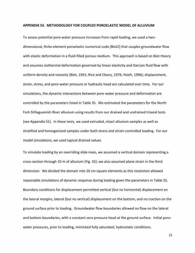
APPENDIX S3. METHODOLOGY FOR COUPLED POROELASTIC MODEL OF ALLUVIUM

To assess potential pore-water pressure increases from rapid loading, we used a two-

dimensional, finite-element poroelastic numerical code (Biot2) that couples groundwater flow

with elastic deformation in a fluid-filled porous medium. This approach is based on Biot theory

and assumes isothermal deformation governed by linear elasticity and Darcian fluid flow with

uniform density and viscosity (Biot, 1941; Rice and Cleary, 1976; Hsieh, 1996); displacement,

strain, stress, and pore-water pressure or hydraulic head are calculated over time. For our

simulations, the dynamic interactions between pore-water pressure and deformation are

controlled by the parameters listed in Table S5. We estimated the parameters for the North

Fork Stillaguamish River alluvium using results from our drained and undrained triaxial tests

(see Appendix S1). In these tests, we used extruded, intact alluvium samples as well as

stratified and homogenized samples under both stress and strain-controlled loading. For our

model simulations, we used typical drained values.

To simulate loading by an overriding slide mass, we assumed a vertical domain representing a

cross-section through 10 m of alluvium (Fig. S5); we also assumed plane strain in the third

dimension. We divided the domain into 10 cm square elements as this resolution allowed

reasonable simulations of dynamic response during loading given the parameters in Table S5.

Boundary conditions for displacement permitted vertical (but no horizontal) displacement on

the lateral margins, lateral (but no vertical) displacement on the bottom, and no traction on the

ground surface prior to loading. Groundwater flow boundaries allowed no flow on the lateral

and bottom boundaries, with a constant zero pressure head at the ground surface. Initial pore-

water pressures, prior to loading, mimicked fully saturated, hydrostatic conditions.

22

We simulated dynamic transit of a moving landslide across the domain by applying a known

vertical traction to the top face of each ground-surface element in sequence from the left

boundary to the right (i.e., simulating landslide loading from north to south). The propagation

of the loading front replicated a landslide speed of 10 m/s (estimated from a runout distance of

approximately 1000 m for the majority of the landslide materials over a period of 100 seconds

(Iverson et al., 2015)). In a single simulation, each 10-cm ground-surface element was

sequentially loaded by 100 kPa (equivalent to the vertical loading from about 5 m of saturated

slide material with a unit weight of 20 kN/m3) over 0.01 s. During this short time, the load at

that element increased linearly from zero to the maximum (100 kPa), then remained at the full

load as the simulated front moved forward to the next element. The simulations did not

include transient impact loading or boundary stresses modified by slide velocity. Dynamic

loading caused the sediment to deform and pore-water pressures to increase from hydrostatic.

Pore pressures could dissipate upward from the unloaded ground surface immediately in front

of the simulated overriding slide mass; however, they were not permitted to dissipate into the

overriding mass, as this was assumed to be much less permeable than the alluvium.

We performed sensitivity tests to examine the relative importance of different sediment

parameters. All parameters could modify simulated pore-pressure responses, but values of

shear modulus and hydraulic conductivity exerted stronger influences. Nevertheless, the

overall patterns of pore-pressure response were similar given reasonable variations in

parameters (Table S5). Modifying the thickness of alluvium to 5 m also did not greatly change

the responses. The amount of vertical traction applied (i.e., loading from increased overriding

23

landslide thickness) did have a profound influence on pore-pressure responses, with pressures

increasing in an approximately linear manner to the applied load.

24

TABLE S5. ALLUVIUM PARAMETERS USED IN BIOT MODELING

Parameter* Units Laboratory test values Biot

model value Average Maximum Minimum

# of meas.

Porosity N.A.† 0.457 0.467 0.445 7 0.46

Drained Poisson ratio§ N.A. 0.37 0.5 0.12 3 0.37

Drained elastic modulus§ N/m2 2.12×107 3.00×107 1.60×107 3 2.1×107

Drained shear modulus# N/m2 7.74×106 1.09×107 5.84×106 3 7.7×106

Saturated hydraulic conductivity

m/s 4.75×10-5 7.00×10-5 2.46×10-5 4 4.8×10-5

Specific weight of water N/m3 N.A. N.A. N.A. N.A. 9.8×103

Bulk modulus of water N/m2 N.A. N.A. N.A. N.A. 2.2×109

Alluvium thickness** m 4.1 13.4 0.6 12 10

*Porosity, stiffness parameters, and hydraulic conductivity measured from laboratory tests conducted as part of this investigation.

†N.A. = not applicable. §Determined at 0.5% strain. #Calculated from elastic modulus assuming Poisson ratio of 0.37. **Thickness estimated from SR530 reconstruction boring logs (Fiske, 2014). The alluvium

may be thicker closer to the slide origin.

25

Figure S5. Finite-element domain used for Biot modeling of poroelastic response in alluvium to

vertical loading on the upper surface from an overriding landslide. Domain is 10 m by 10 m

with 10 cm square elements (20 cm elements shown for clarity). Boundary conditions shown

for both displacement and groundwater flow. Vertical load moves laterally over time (at a rate

of 10 m/s) to simulate advancing landslide front - loads at two steps (1 and 3 m) are shown.

26

APPENDIX S4. METHODOLOGY FOR CYCLIC SHEARING LIQUEFACTION EVALUATION

We evaluated cyclic liquefaction shearing potential via the cyclic stress approach (Seed and

Idriss, 1971) as implemented in Kramer (1996) in which the cyclic stress ratio (CSR), as a

mechanism for soil forcing, is compared to the cyclic resistance ratio (CRR), as a measure of soil

resistance to liquefaction. The factor of safety against liquefaction is therefore defined as

CRR/CSR and a value less than 1 indicates probable liquefaction. Although the method is

empirical and was developed for ground shaking resulting from earthquakes, it can serve as a

proxy for other vibratory motions as well (e.g., Hryciw et al., 1990; Pando et al, 2001; Ashford et

al., 2006).

The CRR is calculated from empirical charts relating some form of soil strength to case studies

where liquefaction from cyclic shaking did (and did not) occur. We used standard penetration

test (SPT) data (i.e., N values) collected from underlying North Fork Stillaguamish River alluvium

at the distal ends of the landslide deposit during reconstruction of SR 530 (Fiske, 2014) and

implemented SPT correction factors according to standard methods (e.g., Coduto, 1994, see

Section 4.3) to arrive at an average value of N1,60 = 3 for the uppermost layer of the alluvium (at

approximate 2 m depth) (Table S6). Whereas SPT values in some other boreholes had higher N

values, we selected the data presented in Table S6 as representative of the loosest layer that

was likely capable of liquefying. The four boreholes listed in Table S6 were located along a 1.3

km-long transect across the length of the valley and thus represented a wide cross section of

the alluvial floodplain overridden by the Oso landslide.

27

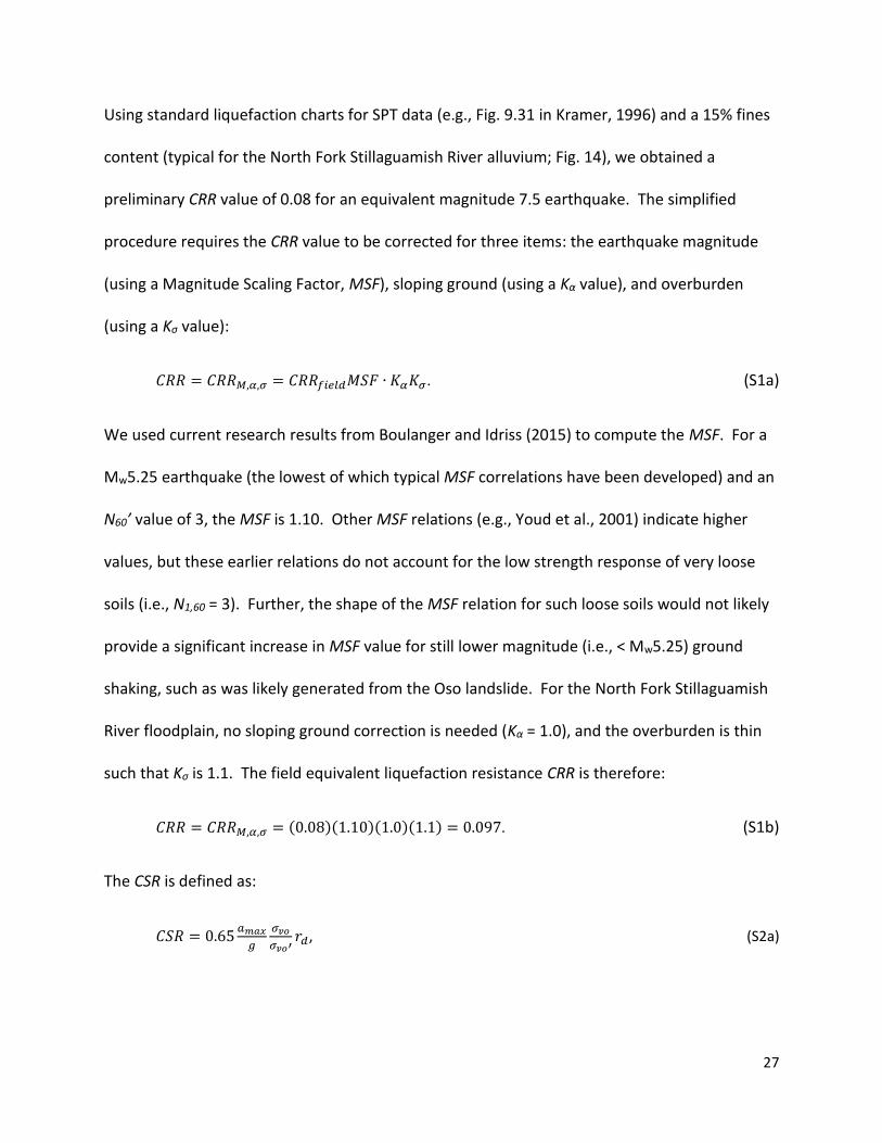
Using standard liquefaction charts for SPT data (e.g., Fig. 9.31 in Kramer, 1996) and a 15% fines

content (typical for the North Fork Stillaguamish River alluvium; Fig. 14), we obtained a

preliminary CRR value of 0.08 for an equivalent magnitude 7.5 earthquake. The simplified

procedure requires the CRR value to be corrected for three items: the earthquake magnitude

(using a Magnitude Scaling Factor, MSF), sloping ground (using a Kα value), and overburden

(using a Kσ value):

𝐶𝑅𝑅 = 𝐶𝑅𝑅𝑀,𝛼,𝜎 = 𝐶𝑅𝑅𝑓𝑖𝑒𝑙𝑑𝑀𝑆𝐹 ∙ 𝐾𝛼𝐾𝜎. (S1a)

We used current research results from Boulanger and Idriss (2015) to compute the MSF. For a

Mw5.25 earthquake (the lowest of which typical MSF correlations have been developed) and an

N60’ value of 3, the MSF is 1.10. Other MSF relations (e.g., Youd et al., 2001) indicate higher

values, but these earlier relations do not account for the low strength response of very loose

soils (i.e., N1,60 = 3). Further, the shape of the MSF relation for such loose soils would not likely

provide a significant increase in MSF value for still lower magnitude (i.e., < Mw5.25) ground

shaking, such as was likely generated from the Oso landslide. For the North Fork Stillaguamish

River floodplain, no sloping ground correction is needed (Kα = 1.0), and the overburden is thin

such that Kσ is 1.1. The field equivalent liquefaction resistance CRR is therefore:

𝐶𝑅𝑅 = 𝐶𝑅𝑅𝑀,𝛼,𝜎 = (0.08)(1.10)(1.0)(1.1) = 0.097. (S1b)

The CSR is defined as:

𝐶𝑆𝑅 = 0.65𝑎𝑚𝑎𝑥

𝑔

𝜎𝑣𝑜

𝜎𝑣𝑜′𝑟𝑑, (S2a)

28

where amax is the peak ground acceleration (pga), g is the gravitational constant (9.81 m/s2), σvo

and σvo’ are the total and effective vertical overburden stress at the depth of interest, and rd is a

depth reduction factor.

We computed amax at the site by scaling seismometer data recorded at a station 11.5 km from

the Oso landslide (Pacific Northwest Seismic Network, Station JCW -

https://pnsn.org/seismogram/current/jcw with data available from

https://service.iris.edu/irisws/timeseries/1/). During the Oso landslide, the pga (vertical

motion only) was 6.53×10-4 m/s2. To scale this data to the Oso site, we compared seismologic

records collected at three USGS “spider” units (OSO1, OSO2, OSO3, data available from USGS

upon request) placed at the slide in the days following the landslide as part of USGS efforts to

monitor ongoing landslide motion during the rescue and recovery efforts. The spiders recorded

several small mass movement events in the weeks that followed the landslide; these included a

till fall on 25 April 2014 when a piece of the headscarp was observed to first slide and then fall

onto the rotated block of the Whitman slide. The impacts made by this event were recorded

both at the spiders and at the JCW station, thereby allowing a scaling correction factor to be

computed for the pga recorded between these stations (K. Allstadt, pers. comm.). During the

sliding motion of the 25 April 2014 till fall, the Oso spiders recorded pga values between 0.03

and 0.10 m/s2. During the falling motion, the spiders recorded pga values between 0.25

m/s2and 0.28 m/s2. At JCW, the sliding and falling motions could similarly be distinguished,

with pga values of 7.37×10-5 m/s2 and 1.22×10-4 m/s2, respectively. Neglecting the sliding

portion of the time series for the OSO1 spider (which appeared to have anomalous data), we

calculated resultant pga ratios (Oso spider/JCW) of 1,259 for sliding and 2,174 (a minimum

29

value due to inadvertent clipping of the source record) for falling. Multiplying these ratios by

the pga value of the JCW record during the Oso landslide results in pga (amax) values of 0.822

m/s2 using the sliding ratio and 1.42 m/s2 using the falling ratio. As the Oso landslide was

primarily a sliding motion, we used the sliding (and lower value) of amax for our calculation of

CSR.

We computed σvo and σvo’ at 2 m depth using a total unit weight of 18.9 kN/m3, assuming full

saturation and based on specific gravity and void ratio from undisturbed samples of river

alluvium (Appendix S1, Table S2 – surface alluvium). This yielded an effective-stress ratio (𝜎𝑣𝑜

𝜎𝑣𝑜′)

equal to 2.08. Finally, for near-surface conditions, no depth reduction factor was needed and rd

was therefore 1.0 (Seed and Idriss, 1971). Putting these components together into equation

S2a resulted in:

𝐶𝑆𝑅 = 0.650.822

9.81

37.8

18.21.0 = 0.113. (S2b)

Calculating the factor of safety (Fs) against liquefaction:

𝐹𝑠 =𝐶𝑅𝑅

𝐶𝑆𝑅= 0.9, (S3)

thereby indicates (i.e., Fs < 1) that liquefaction could have occurred under these ground and

vibration conditions.

30

TABLE S6. SPT DATA OF ALLUVIUM IN THE VICINITY OF STATE ROUTE 530 (SR530) RECONSTRUCTION

Borehole SPT N value*

Depth (m)

Efficiency (%)

SPT N60 value†

Overburden corr. factor

CN§

SPT N1,60 value

E-1-14 0 2.0 83.8 0 1.37 0

C-2-14 2 2.4 90.1 2 1.35 3

C-4p-14 0 1.5 83.8 0 1.40 0

C-5p-14 6 1.0 83.8 6 1.43 9

Average N.A.# N.A. N.A. N.A. N.A. 3

*SPT N values are from Fiske (2014). †SPT correction factors are: CB=1.0 for 10-11 cm (4.0-4.5 inch) borehole, CS=1.0 for

standard sampler, CR=0.75 for 3.3 m (10 ft) rod length. §CN correction factor calculated using Skempton (1986) based on depth and a 18.9

kN/m3 unit weight for either normally consolidated fine or coarse sand in the alluvial sediment.

#N.A. = not applicable.

31

APPENDIX REFERENCES

Amini, F. and Qi, G.Z., 2000, Liquefaction testing of stratified silty sands: Journal of Geotechnical

and Geoenvironmental Engineering, v. 126, no. 3, p. 208-217.

Ashford, S.A., Juirnarongrit, T., Sugano, T., and Hamada, M., 2006, Soil–pile response to blast-

induced lateral spreading. I: field test: Journal of Geotechnical and Geoenvironmental

Engineering, v. 132, no. 2, p. 152-162, doi: 10.1061/(ASCE)1090-0241(2006)132:2(152).

ASTM D422-63, 2007, Standard test method for particle-size analysis of soils: West

Conshohocken, Pennsylvania, ASTM International, www.astm.org.

ASTM D854-14, 2014, Standard test methods for specific gravity of soil solids by water

pycnometer: West Conshohocken, Pennsylvania, ASTM International, www.astm.org.

ASTM D2216-10, 2010, Standard test methods for laboratory determination of water (moisture)

content of soil and rock by mass: West Conshohocken, Pennsylvania, ASTM International,

www.astm.org.

ASTM D2487-11, 2011, Standard practice for classification of soils for engineering purposes

(Unified Soil Classification System): West Conshohocken, Pennsylvania, ASTM

International, www.astm.org.

ASTM D4318-10e1, 2010, Standard test methods for liquid limit, plastic limit, and plasticity

index of soils: West Conshohocken, Pennsylvania, ASTM International, www.astm.org.

32

ASTM D7263-09, 2009, Standard test methods for laboratory determination of density (unit

weight) of soil specimens: West Conshohocken, Pennsylvania, ASTM International,

www.astm.org.

Badger, T.C., 2016, SR 530 Landslide Geotechnical Study: Olympia, Washington, Washington

State Department of Transportation Geotechnical Data Report, May 2016, 355p.

Biot, M.A., 1941, General theory of three-dimensional consolidation: Journal of Applied Physics

v. 12, p. 155-164.

Boulanger, R.W., and Idriss, I.M., 2015, Magnitude scaling factors in liquefaction triggering

procedures: Soil Dynamics and Earthquake Engineering, v. 79, no. B, p. 296-303,

doi:10.1016/j.soildyn.2015.01.004.

Coduto, D.P., 1994, Foundation design, principles and practices: Englewood Cliffs, New Jersey,

Prentice Hall, 796 p.

Cubrinovski, M. and Ishihara, K., 2002, Maximum and minimum void ratio characteristics of

sands: Soils and Foundation, v. 42, no. 6, p. 65-78.

Fiske, A.J., 2014, SR 530 Skaglund Hill Vic. To C-Post Rd. Vic. Emergency Roadway

Reconstruction: Washington State Department of Transportation Geotechnical Data Report

(DMA-153, MP36.8-38.4), May 7, 2014, 138 p.

Hryciw, R.D., Vitton, S., and Thomann, T.G., 1990, Liquefaction and flow failure during seismic

exploration: Journal of Geotechnical Engineering, v. 116, no. 12, p. 1881-1899,

doi:10.1061/(ASCE)0733-9410(1990)116:12(1881).

33

Hsieh, P.A., 1996, Deformation-induced changes in hydraulic head during ground-water

withdrawal: Ground Water, v. 34, p. 1082-1089.

Iverson, R.M., George, D.L., Allstadt, K., Reid, M.E., Collins, B.D., Vallance, J.W., Schilling, S.P.,

Godt, J.W., Cannon, C.M., Magirl, C.S., Baum, R.L., Coe, J.A., Schulz, W.H., and Bower, J.B.,

2015, Landslide mobility and hazards—implications of the 2014 Oso disaster: Earth and

Planetary Science Letters, v. 412, p. 197-208, http://dx.doi.org/10.1016/j.epsl.2014.12.020.

Jefferies M. and Been K., 2015, Soil liquefaction: a critical state approach: Boca Raton, CRC

Press, 2nd Edition, 712 p.

JIS, 2000. Test method for minimum and maximum densities of sands. Japanese Geotechnical

Society, Soil Testing Standards, Japanese Standards Association: JIS A 1224:2000, p. 136–

138 (in Japanese, translated to English by Y. Hosono).

Kramer, S.L., 1996, Geotechnical earthquake engineering: Upper Saddle River, New Jersey

Prentice Hall, 653 p.

Lade, P.V., 2016, Triaxial testing of soils: West Sussex, UK, Wiley, 402 p.

Magirl, C.S., Keith, M.K., Anderson, S.W., O’Connor, J.E., Aldrich, Robert, and Mastin, M.C.,

2015, Preliminary assessment of aggradation potential in the North Fork Stillaguamish

River downstream of the State Route 530 landslide near Oso, Washington: U.S. Geological

Survey Scientific Investigations Report 2015–5173, 20 p.,

http://dx.doi.org/10.3133/sir20155173.

34

Mulilis, J.P., Arulanandan, K., Mitchell, J.K., Chan, C.K. Seed, H.B., 1977, Effects of sample

preparation on sand liquefaction, Journal of the Geotechnical Engineering Division, ASCE,

Vol. 103, No. 2, p. 91-108.

Pando, M.A., Olgun, C.G., and Martin, J.R. II, 2001, Liquefaction potential of railway

embankments: Missouri University of Science and Technology, International Conferences

on Recent Advances in Geotechnical Earthquake Engineering and Soil Dynamics, paper no.

2.29, 6 p., http://scholarsmine.mst.edu/icrageesd/04icrageesd/session02/16.

Rice, J.R. and Cleary, M.P., 1976, Some basic stress diffusion solutions for fluid-saturated elastic

porous media with compressible constituents: Reviews of Geophysics, v. 14, no. 2, p. 227-

241.

Seed, H.B. and Idriss, I.M., 1971, Simplified procedure for evaluating soil liquefaction potential:

Journal of the Soil Mechanics and Foundations Division (American Society of Civil

Engineers), v. 97, p. 1249-1273.

Skempton, A.W., 1986, Standard penetration test procedures and the effects in sands of

overburden pressure, relative density, particle size, aging and overconsolidation:

Géotechnique, v. 36, no. 3, p. 425-447.

Terzaghi, K., Peck, R. B., and Mesri, G., 1996, Soil mechanics in engineering practice: New York,

John Wiley & Sons, 549 p.

Wood, D.M., 1991, Soil behaviour and critical state soil mechanics: Cambridge, Cambridge

University Press, 488 p.

35

Youd, T.L. and others, 2001, Liquefaction resistance of soils: summary report from the 1996

NCEER and 1998 NCEER/NSF workshops on evaluation of liquefaction resistance of soils:

Journal of Geotechnical and Geoenvironmental Engineering, v. 127, no. 10, p. 817-833,

doi:10.1061/(ASCE)1090-0241(2001)127:10(817).