Data Quality Considerations for Big Data and Machine

1

Data Quality Considerations for Big Data and

Machine Learning: Going Beyond Data Cleaning and

TransformationsVenkat N. Gudivada∗, Amy Apon†, and Junhua Ding∗

∗Department of Computer Science, East Carolina University, USA†School of Computing, Clemson University, USA

email: [email protected], [email protected], and [email protected]

Abstract—Data quality issues trace back their originto the early days of computing. A wide range of domain-specific techniques to assess and improve the quality of dataexist in the literature. These solutions primarily target datawhich resides in relational databases and data warehouses.The recent emergence of big data analytics and renaissancein machine learning necessitates evaluating the suitabilityrelational database-centric approaches to data quality. In thispaper, we describe the nature of the data quality issues in thecontext of big data and machine learning. We discuss facetsof data quality, present a data governance-driven frameworkfor data quality lifecycle for this new scenario, and describean approach to its implementation. A sampling of the toolsavailable for data quality management are indicated andfuture trends are discussed.

Keywords-Data Quality; Data Quality Assessment ; DataCleaning; Big Data; Machine Learning; Data Transformation

I. Introduction

This paper is a substantial extension of the work

presented at the ALLDATA 2016 conference [1]. Data

quality plays a critical role in computing applications

in general, and data-intensive applications in particular.

Data acquisition and validation are among the biggest

challenges in data-intensive applications. High-quality

data brings business value in the form of more informed

and faster decisions, increased revenues and reduced

costs, increased ability to meet legal and regulatory com-

pliance, among others. What is data quality? It depends

on the task and is often defined as the degree of data fit-

ness for a given purpose. It indicates the degree to which

the data is complete, consistent, free from duplication,

accurate and timely for a given purpose.

The application of relevant practices and controls

to improve data quality is referred to as data quality

management. Defining and assessing data quality is a

difficult task as data is captured in one context and

used in totally different contexts. Furthermore, the data

quality assessment is domain-specific, less objective, and

requires significant human involvement.

A. Ubiquity of Data Quality Concerns

Data quality is a concern in many application do-

mains. Consider the software engineering domain. The

effectiveness of prediction models in empirical software

engineering critically depends on the quality of the data

used in building the models [2]. Data quality assessment

plays a critical role in evaluating the usefulness of data

collected from the Team Software Process frameworks [3]

and empirical software engineering research [4]. Cases In-

consistency Level (CIL) is a metric for analyzing conflicts

in software engineering datasets [5].

Data quality is studied in numerous other domains

including cyber-physical systems [6], assisted living sys-

tems [7], citizen science [8], ERP systems [9], accounting

information systems [10], drug databases [11], smart

cities [12], sensor data streams [13], linked data [14],

data integration [15], [16], multimedia data [17], scien-

tific workflows [18], and customer databases [19]. big

data management [20], Internet of Things (IoT) [21], and

machine learning [22] domains are generating renewed

interest in data quality research. A wide range of domain-

specific techniques to assess and improve the quality of

data exist in the literature [23], [24], [25].

B. Manifestations of Lack of Data Quality

Lack of data quality in the above domains man-

ifests in several forms including data that is missing,

incomplete, inconsistent, inaccurate, duplicate and dated.

Though the data quality issues date back to the early days

of computing, many organizations struggle with these

basic elements of data quality even today. For example,

capturing and maintaining current and accurate customer

data is largely an expensive and manual process. Achiev-

ing an integrated and single view of customer data which

is gleaned from several sources remains elusive and

expensive.

Organizations often overestimate data quality and

underplay the implications of poor quality data. The

consequences of bad data may range from significant to

catastrophic. Data quality problems can cause projects

to fail, result in lost revenues and diminished customer

relationships, and customer turnover. Organizations are

routinely fined for not having an effective regulatory

compliance process. High-quality data is at the heart of

regulatory compliance. The Data Warehousing Institute

1

International Journal on Advances in Software, vol 10 no 1 & 2, year 2017, http://www.iariajournals.org/software/

2017, © Copyright by authors, Published under agreement with IARIA - www.iaria.org

(TDWI) estimates that poor data quality costs businesses

in the United States over $700 billion annually [26].

C. Dual Threads of Data Quality Research

Data quality research is primarily advanced by

computer science and information systems researchers.

Computer science researchers address data quality issues

related to the identification of duplicate data, resolving

inconsistencies in data, imputation for missing data, link-

ing and integrating related data obtained from multiple

sources [24]. Computer scientists employ algorithmic

approaches based on statistical methods to address the

above issues [27]. Information systems researchers, on

the other hand, study data quality issues from a systems

perspective [28]. For example, they investigate the contri-

bution of user interfaces towards data quality problems.

Though statisticians also confront data quality issues, the

magnitude of their datasets pale in comparison to big

data and machine learning environments.

D. Operational Data-centric Data Quality Research

Traditionally, data quality research has been exclu-

sively focused on operational data — business transac-

tions [29]. This data is structured and is typically stored

in relational databases. Integrity constraints have been

used as the primary mechanism to enforce data qual-

ity. This approach is effective in preventing undesirable

changes to data that is already in the database. It does

not address issues that originate at the source such as

missing, incomplete, inaccurate, and outlier data.

Operational data alone is inadequate to support the

needs of an organization-wide strategic decision making.

Data warehouses were introduced to fill this gap. They

extract, clean, transform, and integrate data from mul-

tiple operational databases to create a comprehensive

database. A set of tools termed Extract, Transform, and

Load (ETL) are used to facilitate construction of data

warehouses. The data in the warehouses is rarely updated

but refreshed periodically, and is intended for a read-only

mode of operation. Data warehouse construction calls for

an extreme emphasis on ensuring data quality before the

data is loaded into the warehouse.

Compared to database environments, data ware-

houses pose additional challenges to data quality. Since

data warehouses integrate data from multiple sources,

quality issues related to data acquisition, cleaning, trans-

formations, linking, and integration becomes critical. Sev-

eral types of rules and statistical algorithms have been

devised to deal with missing data, identification of dupli-

cates, inconsistency resolution, record linking, and outlier

detection [30].

As a natural progression, subsequent data qual-

ity research encompassed web data sources. Evaluating

the veracity of web data sources considers quality of

hyperlinks, browsing history, and factual information

provided by the sources [31]. Other investigations used

relationships between web sources and their information

for evaluating veracity of web data [32].

E. Big Data and Machine Learning Exacerbate Data Qual-

ity Concerns

The recent rise and ubiquity of big data have ex-

acerbated data quality problems [20]. Streaming data,

data heterogeneity, and cloud deployments pose new

challenges. Furthermore, provenance tracking is essential

to associate a degree of confidence to the data [33],

[34]. To address the storage and retrieval needs of di-

verse big data applications, numerous systems for data

management have been introduced under the umbrella

term NoSQL [35]. Unlike the relational data model for

the operational databases and the star schema-based

databases for data warehousing, NoSQL systems feature

an assortment of data models and query languages [36].

In the current NoSQL systems, performance at scale

takes precedence over data quality. In other words, near

real-time processing overshadows everything else. Fur-

thermore, database schema evolution is celebrated as a

desirable feature of certain classes of NoSQL systems.

Recently, many organizations have begun imple-

menting big data-driven, advanced and real-time analyt-

ics for both operational and strategic decision making.

Machine learning algorithms are the foundation for such

initiatives, especially for the predictive and prescriptive

analytics [37]. However, poor data quality is the major

factor impeding advanced analytics implementations [38].

It is often said that the biggest challenge for big data is

the quality of big data itself.

In contrast with big data, Machine Learning (ML)

presents a different set of data quality concerns. The

three components of ML algorithms are model represen-

tation, measures for assessing model accuracy, and meth-

ods for searching for a best model in the model space

(i.e., optimization). As these three components are tightly

intertwined, assessing data quality for ML applications

is a complex task. For example, applications for which

the linear model is the right model, a small number of

representative data/observations will suffice for model

building and testing. Even if we use an extremely large

number of observations to build a linear model, it may

not help the model performance. On the other hand,

consider an application such as a self-driving car. By late

2016, Google’s self-driving car program logged 2 million

miles, which was aggregated from 60 vehicles. Still this

data does not sufficiently capture different scenarios that

depict the complexities of driving on diverse roads under

various weather conditions. Such datasets are said to be

computationally large, but statistically sparse.

There seems to a belief that more data compensates

for using less sophisticated ML models. The current

best practices suggest that more data and better models

produce superior results. Moreover, a model developed

using a stratified sampling performs as good or even

better than a model that is built using all the data.

Furthermore, for the same feature set, a more complex

model such as a non-linear model does not perform any

better than a simpler model such as the linear model.

2



However, more complex models when coupled with more

complex features yield significantly better performance.

In machine learning, often the raw data is not in

a form that is suitable for learning. Variables/features

are identified and extracted from the raw data. Though

features tend to be domain-specific, there is a need to

establish generic patterns that help identify the features.

Lack of data quality manifested in the form of

missing data, duplicate data, highly correlated variables,

large number of variables, and outliers. Poor quality data

can pose significant problems for building ML models as

well as big data applications. Statistical techniques such

as missing data imputation, outlier detection, data trans-

formations, dimensionality reduction, robust statistics,

cross-validation and bootstrapping play a critical role in

data quality management.

F. Organization of the Paper

The overarching goal of this paper is to describe the

nature of the data quality issues and their characteriza-

tion in the context of big data and machine learning. We

discuss facets of data quality, present a data governance-

driven framework for data quality lifecycle for this new

scenario, and describe an approach to its implementation.

More specifically, data quality issues in the context of big

data and machine learning are discussed in Sections II

and III. In Section IV, we present data quality case studies

to highlight the significance of data quality in three di-

verse applications. These three case studies are expected

to motivate the problem and illustrate the complexity of

data quality issues.

Next, we define data quality more concretely in

terms of several dimensions (aka facets) in Section V. A

data governance-driven data quality lifecycle is described

in Section VI. A reference framework based on the lifecy-

cle for data quality and its implementation are described

in Section VII. A sampling of the tools available for

data quality management are mentioned in Section VIII.

Future trends are discussed in Section IX and Section X

concludes the paper. To help the readers who are not

familiar with machine learning, appendices A, B, C, and

D introduce essential machine learning concepts, outliers,

robust statistics, and dimensionality reduction, from a

data quality perspective.

II. Data Quality Challenges in Big Data

Data quality is a problem that has been studied

for several decades now. However, primarily the focus

has been on the data in operational databases and data

warehouses. Only recently, researchers have begun inves-

tigating data quality issues beyond the operational and

warehousing data. Unlike the case of relational databases,

NoSQL systems for big data employ a wide assortment of

data models. The attendant question is: Do we need a sep-

arate data quality management approach for each NoSQL

system? In big data and machine learning domains, data

is acquired from multiple vendors. Data is also gener-

ated by crowd-sourcing, which is complemented by user-

contributed data through mobile and web applications.

How do we assess the veracity and accuracy of crowd-

sourced and user-contributed data?

The proliferation of digital channels and mobile

computing is generating more data than ever before.

What is the impact of cloud deployments on data quality?

Should data quality investigations move beyond column

analysis in relational databases and address issues re-

lated to complex data transformations, integration of

data from diverse data sources, and aggregations that

provide insights into data?

A. Confounding Factors

Data quality in big data is confounded by multiple

factors. Some big data is collected through crowdsourcing

and these projects are not open for public comments and

scrutiny. Also, for the machine-generated data, sufficient

meta data is often not available to evaluate the suitabil-

ity of data for a given task. Furthermore, vendors use

multiple approaches for data collection, aggregation, and

curation without associating any context for downstream

data usage. However, the context plays a central role in

determining data suitability for tasks. For example, the

types of sampling methods used in data collection deter-

mine the valid types of analyses that can be performed

on the data.

B. Dealing with Missing Data

Missing data is a major concern in big data. From a

statistical perspective, missing data is classified into one

of the three categories: Missing Completely At Random

(MCAR), Missing At Random (MAR), Missing Not At Ran-

dom (MNAR) [39]. In MCAR, as the name implies, there

is no pattern to the missing data. Data is missing inde-

pendently of both observed and unobserved data. The

missing and observed values have similar distributions.

In other words, MCAR is just a subset of the data.

MAR is a misnomer and another name like Missing

Conditionally at Random better captures its meaning.

Given the observed data, data is missing independently of

unobserved data. It is possible that there are systematic

differences between the missing and observed values,

and these differences can entirely be explained by other

observed variables. MCAR implies MAR, but vice versa.

In MNAR, missing observations are related to the unob-

served data. Therefore, observed data is a biased sample.

High rates of missing data require careful attention,

regardless of the analysis method used. If MCAR and

MAR cases prevail for a variable, such variables can be

dropped across all observations in the dataset. However,

dropping MNAR variables may lead to results that are

strongly biased.

Several approaches exist for dealing with missing

data. The simplest approach is to delete from the dataset

3



all observations that have missing values. If a large pro-

portion of observations have missing values for a critical

attribute, its deletion will have an effect on the statistical

power. A variation of the above approach is called pair-

wise deletion. Assume that a dataset has three variables,

v1, v2, v3, and some observations have missing values for

the attribute v2. The entire dataset can be included for

analysis by a statistical method if the method does not

use v2. Pairwise deletion allows more of the data in the

dataset be used in the analysis. However, each computed

statistic may be based on a different subset of observa-

tions in the dataset. A correlation matrix computed using

pairwise deletion may have negative eigenvalues, which

can cause problems for certain statistical analyses.

Another approach to missing data is mean sub-

stitution. The mean may be calculated for a group of

observations (e.g., customers who are based in a spe-

cific geographic region) or the entire dataset. Predicting

missing values using multiple regression on a set of

highly correlated variables is another approach. However,

this method may entail overfitting for big data machine

learning. Lastly, multiple imputation approach is also

used for predicting missing values. Methods such as

expectation-maximization (EM)/ maximum likelihood es-

timation, Markov Chain Monte Carlo (MCMC) simulation,

and propensity score estimation are used to estimate the

missing values. A version of the dataset corresponding to

each method is created. The datasets are then analyzed

and the results are combined to produce estimates and

confidence intervals for the missing values.

C. Dealing with Duplicate Data

Identifying and eliminating duplicate data is critical

to big data applications. Duplicates are ubiquitous espe-

cially in user-contributed data in social network applica-

tions. For example, a user may unintentionally create a

new profile without recognizing that her profile already

exists. As a result, she may receive multiple notifications

for the same event. Householding is closely related to

deduplication, and involves identifying all addresses that

belong to the same household. Householding obviates

the need for sending the same information to multiple

addresses of the same family.

Identifying duplicate data is a difficult task in the

big data context. There are two major issues. The first

is assigning a unique identifier to various pieces of

information that belong to the same entity. The unique

identifier is used to aggregate all information about the

entity. This process is also referred to as linking. The

second issue is identifying and eliminating duplicate

data based on the unique identifiers. Given the volume

of data, duplicate elimination is resource-challenged as

data is too big to fit in main memory all at once. One

solution is to use the Bloom filter, which requires that the

associated hash functions be independent and uniformly

distributed. Bloom filter is a space-efficient probabilistic

data structure for testing set membership.

D. Dealing with Data Heterogeneity

Big data is often characterized by five Vs: volume,

velocity, variety, veracity, and value. It is especially the

variety (aka data heterogeneity) that poses greatest chal-

lenges to data quality. Data heterogeneity is manifested

as unstructured, semi-structured, and structured data

of disparate types. Traditionally, data quality research

focused on structured data which is stored in relational

databases. The emergence and the ubiquity of Web data

attracted researchers to tackle data quality issues associ-

ated with semi-structured data in the Web pages [31].

Information extraction (IE) refers to synthesizing

structured information such as entities, attributes of

entities, and relationships among the entities from un-

structured sources [40]. IE systems have evolved over

the last three decades from manually coded rule-based

systems, generative models based on Hidden Markov

Models, conditional models based on maximum entropy,

methods that perform more holistic analysis of docu-

ments’ structures using grammars, to hybrid models that

leverage both statistical and rule-based methods. Most

of the IE research targets textual data such as natural

language texts. Another line of IE research focuses on

extracting text present in images and videos [41]. The

next level of IE is to extract information from images

and video (aka feature detection and feature extraction),

which is extremely difficult and context dependent. IE

data quality challenges primarily stem from the uncer-

tainty associated with the extracted information.

E. Semantic Data Integration

As big data is typically loosely structured and often

incomplete, most of it essentially remains inaccessible

to users [15]. The next logical step after information

extraction is to identify and integrate related data to

provide users a comprehensive, unified view of data.

Integrating unstructured heterogeneous data remains a

significant challenge. Initiatives such as the IEEE’s Smart

Cities and IBM’s Smarter Cities Challenge critically de-

pend on integrating data from multiple sources. The

difficulties of information extraction and data integra-

tion, and attendant data quality issues are manifested

in operational systems such as Google Scholar, Citeseer,

ResearchGate, and Zillow.

III. Data Quality Challenges in Machine Learning

Traditionally, data quality is assessed before using

the data. In contrast, in the machine learning context,

quality is assessed before the model is built as well as

after. Data quality is assessed before model building us-

ing a set of dimensions (see Section V). The effectiveness

of a model is evaluated using another subset of the data

which was not used for model building. Performance of

machine learning models is used as an indirect measure

of data quality. Certain pre-processing operations on the

data help these models achieve increased effectiveness.

4



Readers who are not familiar with machine learning

concepts are encouraged to consult Appendix A before

reading further.

High-quality datasets are essential for developing

machine learning models. For example, outliers in train-

ing dataset can cause instability or non-convergence in

ensemble learning. Incomplete, inconsistent, and miss-

ing data can lead to drastic degradation in prediction.

The data available for building machine learning models

is usually divided into three non-overlapping datasets:

training, validation, and test. The machine learning model

is developed using the training dataset. Next, the valida-

tion dataset is used to adjust the model parameters so

that overfitting is avoided. Lastly, the test dataset is used

to evaluate the model performance.

A. Bias and Variance Tradeoff in Machine Learning

Machine learning models are assessed based on

how well the they predict response when provided with

unseen input data, which is referred to as prediction

accuracy, or alternatively, prediction error. Three sources

contribute to prediction error: bias, variance, and irre-

ducible error. Bias stems from using an incorrect model.

For example, a linear algorithm is used when a nonlinear

one fits the data better for a classification problem.

Bias is the difference between the expected value and

predicted value. The linear model will have high bias since

it is unable to learn the nonlinear boundary between the

classes. High bias would produce consistently incorrect

results.

The variance is an error which arises due to small

fluctuations in the training dataset. In other words, the

variance is the sensitivity of a model to changes to

the training dataset. Decision trees, for example, learned

from different datasets for the same classification prob-

lem will have high variance. In contrast, decision trees

have low bias since they can represent any Boolean func-

tion. In other words, the trees can fit to the training data

well by learning appropriate Boolean functions associated

with the tree internal nodes.

A popular way to visualize bias and variance trade-

off is through a bulls-eye diagram shown in Figure 1.

The innermost circle is the bulls-eye and this region

represents the expected values. When both the bias and

variance are low, the expected values and the predicted

values do not differ significantly (top-left concentric cir-

cles). When the variance is low but the bias is high, the

predicted values are consistently differ from the expected

values. For the low bias and high variance case, some pre-

dicted values are closer to the expected values. However,

the difference between the expected and predicted values

vary considerably. Lastly, when both the bias and the

variance are high, the predicted values are off from the

expected values and the difference between the expected

and predicted values vary widely.

The irreducible error is due to the noise in the

problem itself and cannot be reduced regardless of which

algorithm is employed.

Bias and variance compete with each other and

simultaneously minimizing these two sources of error is

not possible. This is referred to as bias-variance trade-

off. This applies to all supervised learning algorithms and

prevents them from generalizing beyond their training

datasets. Generally, parametric models have higher bias,

but low variance. They make more assumptions about

the form of the model. They are easy to understand,

but deliver low predictive performance. In contrast, non-

parametric algorithms make fewer assumptions about the

form of the model, and have low bias but high variance.

B. Cross-validation and Bootstrapping

When the data available for model building and

testing is limited, a technique called cross-validation is

used [22]. Though one may think that this situation does

not arise in big data contexts, availability of sufficiently

high-quality data can be a limiting factor. There are

many variations of cross-validation including leave-one-

out cross-validation (LOOCV) and k−fold cross-validation.

LOOCV splits a dataset of size n into two parts of size 1

and n−1. The n−1 data items are used to build the model

and the remaining data item is used for model evaluation.

This procedure is repeated n−1 times, where a different

data item is used for the evaluation role. The k−fold

cross-validation is a computationally efficient alternative

to LOOCV. It involves randomly dividing the set of data

items into k groups/folds of approximately equal size.

The first fold is used for testing, whereas the remaining

k−1 folds are used to develop the model. This procedure

is repeated k − 1 times, each time a different fold plays

the role of test data.

Another technique to deal with limited data is called

bootstrapping. Assume that we have a small dataset of

size n. A bootstrap sample of size n is produced from the

original dataset by randomly selecting n data items from

it with replacement. Any number of bootstrap samples

of size n can be produced by repeating this process. It

should be noted that some data items may be present

multiple times in the bootstrap sample.

C. Data Transformations

Note that a feature vector has multiple components

and each corresponds to a (predictor) variable. The Linear

Discriminant Analysis (LDA) is a preferred classification

algorithm when the number of classes is more than

two. However, LDA assumes that each variable has the

same variance. For such cases, data is first standard-

ized by applying the z−transform [42]. The mean of

the z−transformed data is always zero. Moreover, if the

original data is distributed normally, the z−transformed

data will conform to a standard normal distribution,

which has a zero mean and a standard deviation of one.

Other machine learning algorithms assume a nor-

mal distribution for variables. For variables that are not

normally distributed, transformations are used to bring

data to normality conformance. Logarithm and square

5



Figure 1: Visualizing bias and variance tradeoff using a bulls-eye diagram

root transformations are appropriate for exponential dis-

tributions, whereas the Box-Cox transformation is better

suited for skewed distributions.

D. Other Considerations

Outliers are values that are drastically different

from rest of the values in a dataset. Outliers may actually

be legitimate data, or the result of sampling bias and

sampling errors. For example, a malfunctioning or non-

calibrated Internet of Things (IoT) device may generate

outliers. Furthermore, outliers are also due to inherent

variability in the data.

In some cases, the number of predictor variables can

be extremely large and the associated problem is known

as dimensionality curse. The k-nearest neighbor (kNN)

algorithm works well when the number of dimensions

of the input vector is small. If this number is high, the

values computed by the distance metric of the algorithm

become indistinguishable from one another. In other

words, as dimensionality increases, the distance to the

nearest neighbor approaches the distance to the farthest

neighbor. The training data, irrespective of its size, cov-

ers only a small fraction of the input space. Therefore,

no training datasets are big enough to compensate for

dimensionality curse.

To overcome the dimensionality curse,

variable/feature reduction techniques are used. Machine

learning models need is a minimal set of independent

variables that are correlated to the prediction, but not

to each other. Variable selection (aka feature selection)

is the process of choosing a minimal subset of relevant

variables that are maximally effective for model building.

Principal Component Analysis (PCA) and Exploratory

Factor Analysis (EFA) are two techniques for variable

selection and dimension reduction. Dimensionality

reduction also occurs when a group of highly correlated

variables is removed and replaced by just anyone

variable in the group. Readers who are not familiar

with detecting and removing outliers, robust statistics,

and dimensionality reduction through PCA and EFA are

referred to Appendices B, C, and D, respectively.

IV. Data Quality Case Studies

In this section, we present three data quality case

studies. Many organizations still depend on manual data

cleansing using methods such as manually reviewing

data in spreadsheets or one-off corrections to bad data.

The current generation data profiling and data quality

assessment tools attest to this statement. The first case

study illustrates the dominance of manual processes and

labor intensive nature of data quality tasks. Machine

learning and big data offer unprecedented opportunities

for automating data quality tasks such as outlier detec-

tion, identification of inaccurate and inconsistent data,

and imputation of missing data. The second and third

case studies illustrate the role of machine learning and

big data in data quality management.

A. InfoUSA

Producing high-quality data requires significant

manual labor. InfoUSA data vendor is a case in point.

InfoUSA sells mailing address data of consumers and

6



businesses. The volume of this data is farther from being

classified as big data. They collect business data from

over 4,000 phone directories and 350 business sources.

Consumer data is gleaned from over 1,000 sources in-

cluding real estate records and voter registration files.

Data quality issues such as inconsistency, incomplete-

ness, missing and duplicate data abound in mailing ad-

dress data. Over 500 InfoUSA full-time employees are

engaged in data collection and curation.

B. Zillow

Zillow is a big data-driven real estate and rental mar-

ketplace. In contrast with InfoUSA, Zillow uses automated

approaches to data acquisition, cleaning, transformation,

integration, and aggregation. Zillow is a living database of

over 110 million homes in the United States. It provides

information about homes that are for sale or rent, and

also homes that are not currently on the market. It is a

living database in the sense that the data is continually

kept current. For example, Zillow provides daily updated

ZestimateÉ for both home values and fair rental values.

ZestimateÉ home valuation is Zillow’s estimated market

value, which is computed using a proprietary formula.

The formula uses both public and user-submitted data

and incorporates undisclosed special features, location,

and local market conditions. ZestimateÉ home valuation

is more accurate for those geographic areas where the

number of real estate transactions is large.

Zillow acquires data through publicly available

sources such as prior and current real estate transactions,

county courthouse real estate deeds and tax assessments.

This data is also integrated with local real estate market

conditions and historical data. ZestimateÉ values are a

measure of Zillow’s data quality accuracy. Across the

entire real estate market, ZestimateÉ has a median error

rate of 4.5% — ZestimateÉ values for half of the homes

in an area are within 4.5% of the selling price, and the

values for the remaining half are off by more than 4.5%.

This is remarkable given that the ZestimateÉ values are

computed by an algorithm without a human in the loop.

Zillow uses machine learning algorithms to auto-

mate data cleaning tasks such as outlier detection, data

matching, and imputation of missing data. It also employs

machine learning algorithms for data transformations,

integration, and aggregation. These algorithms process

20 TB of data about 110 million homes. Each home is

characterized by over 103 attributes. Time series data

about homes encompasses a moving window of most

recent 220 months. As an example, consider the following

information about a home: 2 beds, 20 baths, and 1,000 sq

ft of living space. The number of bathrooms can be easily

detected as incorrect data using a supervised learning

algorithm such as linear regression. Consider another

task of integrating data from multiple sources such as

MLS-1, MLS-2, county records, and user-provided data.

By using weighted text and numeric features, distance

metrics, and the k-nearest neighbor (kNN) machine learn-

ing algorithm, data from several sources can be matched

quite accurately.

C. Determining Duplicate Questions in Quora

Quora is a question-and-answer website where ques-

tions and answers are contributed by users. Questions are

asked, answered, edited and organized by a community

of users. Quora enables users to edit questions collabora-

tively and suggest edits to answers contributed by other

users. Quora uses an internally developed algorithm to

rank answers to questions.

A question can be phrased in many different ways.

Ability to determine if two differently worded questions

are the same is critical to Quora. Such a capability is

useful in directing the question asker to existing answers

immediately. Furthermore, this obviates the need for

Quora to solicit users to answer a question if the answer

already exists for the question.

Recently, Quora released a first public dataset which

is related to the problem of identifying duplicate ques-

tions. This dataset is comprised of over 400,000 lines of

potential question duplicate pairs. A line is comprised of

full text for each question in the pair, unique identifier

for the question, and a binary flag indicating whether or

not the question pair is a duplicate of each other. Quora

ensured that this dataset is balanced – the number of

question pairs that are duplicates is almost the same

as the number of question pairs that are not duplicates.

The goal of this dataset is to encourage natural language

processing and machine learning researchers to find so-

lutions to duplicate detection problem. Along the lines

of Quora Question Pairs, Kaggle Competitions feature

several challenging problems and associated datasets to

advance machine learning research. Though it appears

that model building is the primary activity in these com-

petitions, data preprocessing and data quality assessment

plays an equally important role.

V. Data Quality Dimensions and Assessment

What exactly is data quality? One may define data

quality in terms of its fit for a business purpose. This is a

generic and qualitative definition. To bring concreteness

to the definition, data quality is often measured as a func-

tion of a set of dimensions such as accuracy, currency,

and consistency. A data quality dimension provides a

basis to measure and monitor the quality of data. How-

ever, we need an objective methodology to assess each

dimension. These methodologies may require different

sets of tools and techniques to quantify dimensions.

Therefore, the resources required for each dimension

will also vary. The initial assessment of data quality

will form the baseline. Enhanced data quality resulting

from new data cleaning, transformation, integration, and

aggregation activities is measured against the baseline.

There is no consensus on what comprises the data

quality dimensions. The dimensions proposed in the

literature vary considerably. Also, they are based on the

7



premise that data is primarily stored relational database

management systems (RDBMS) and data warehouses.

However, the advent of big data has brought in numerous

data models and systems for data management under the

umbrella term NoSQL [35].

Table I lists a set of data quality dimensions for

the big data and machine learning contexts, which are

generic and transcend application domains. Some of

these dimensions can be evaluated using an ordinal scale.

For example, consider the Data Governance dimension.

Each question in the description column corresponding

to this dimension is regarded as a sub-dimension. The

latter can be measured using an ordinal scale such as

{No data standards exist, Data standards exist but are

not enforced, Data standards exist and are enforced}.

In contrast, dimensions such as the Data Duplication

can be quantified numerically. For example, the ratio

of the number of duplicate observations to the total

number of observations is one such numerical measure.

Other dimensions such as Outliers require more elaborate

methods for its quantification.

VI. Data Governance-Driven Data Quality Life

Cycle

Data governance is a set of best practices and con-

trols undertaken by an organization to actively manage

and improve data quality. Data governance provides a

process-oriented framework to embed and execute data

quality activities such as planning, cleaning, profiling, as-

sessing, issue tracking, and monitoring. Data governance

identifies clear roles and responsibilities for ensuring

data quality through repeatable processes. Data gover-

nance, though existed for long, is considered as an emerg-

ing discipline given its recent renaissance. Organizations

that do not have an effective data governance, tend to

take a tactical and quick-fix approach to data quality

problems. Data governance, on the other hand, provides

an organization-wide, proactive and holistic approach to

data quality. It strives to capture data accurately and also

enforces controls to prevent deterioration of data quality.

Data governance calls for establishing a data governance

strategy, policies, procedures, roles and responsibilities.

To identify suitable procedures for assessing vari-

ous data quality dimensions and to implement the pro-

cedures, we need to first understand the data quality

lifecycle in a data governance environment. The lifecycle

depicts the movement of data through various processes

and systems in an organization. Shown in Figure 2 is

such a lifecycle suitable for organizations that follow

data governance-driven approach to data management.

The circled numbers in the figure indicate the ordering

of the lifecycle processes.

A. Data Governance Standards

The first component of the data quality lifecycle is

the Data Governance Standards, which is labeled 1© in

Figure 2. There are four processes in this component.

Data Dictionary is a repository of definitions of business

and technical terms. It includes information about con-

ventions for naming data, meaning of data, its origin,

owner, usage, and format. It may also include relation-

ships of a data item to other data elements, default

values, minimum and maximum values. Data dictionar-

ies are also called data glossaries. The data dictionary

counterpart in a relational database management system

is called system catalog, which provides detailed informa-

tion about the logical and physical database structures,

table data statistics, authentication and authorization.

Advanced data dictionaries may also feature those func-

tions provided by taxonomies and ontologies. The data in

the data dictionary is meta data since it describes other

data.

Reference & Meta Data refers to two types of data.

Reference data is any data that can be used to organize,

classify, and validate other data. For example, ISO country

codes are reference data. They are internationally rec-

ognized codes for uniquely identifying countries. Other

reference data include codes for airports, zip codes,

Classification of Instructional Programs (CIP) codes.

Reference data is critical to data validation. For

instance, some data entered by application users can

be validated against reference datasets. Master data is

another category of data, which is often erroneously

equated to the reference data. They are clearly different

though they are interdependent. Master data represents

core business data such as products, services, customers,

and suppliers. It represents entities that come into play

in business transactions such as a customer placing an

order for a product. Meta data refers to additional data

about data whose scope is beyond the data dictionary.

Such meta data is typically generated by other processes

in the data quality framework.

The next process, Data Models & Business Rules, doc-

uments a range of data models and policies. Data models

go beyond the relational data model and may include

NoSQL data models such as column-family and graph

models. Business Rules specify complex relationships be-

tween data elements from a validation perspective. They

also encompass rules for missing data imputation, spot-

ting data integrity violations, resolving inconsistent data,

linking related data, detection of outliers, and purging

dated data, among others.

The last process, Roles & Responsibilities, involves

identifying various roles for data quality management

and associating responsibilities with each role. Roles

may include an owner, program manager, project leader,

chief data officer, business analyst, data analyst, and

data steward. For example, a data analyst’s role may

include addressing issues raised in data quality reports

and tracking resolution of these issues. Responsibilities

associated with each role vary from one organization to

another.

8



TABLE I: Data quality dimensions

Dimension Name Description

Data Governance Do organization-wide data standards exist and are they enforced? Do clearly

defined roles and responsibilities exist for data quality related activities? Does

data governance strive to acquire and maintain high-quality data through proactive

management?

Data Specifications Are data standards documented in the form of a data dictionary, data models,

meta data, and integrity constraints?

Data Integrity How is data integrity maintained? How are data integrity violations detected and

resolved?

Data Consistency If data redundancy exists, how is data consistency achieved? What methods

are used to bring consistency to data that has become inconsistent? If data is

geographically replicated, how is the consistency and latency managed?

Data Currency Is the data current? Do procedures exists to keep the data current and purge stale

data?

Data Duplication Are there effective procedures in place to detect and remove duplicate data?

Data Completeness Is the data about entities complete? How is missing data managed?

Data Provenance Is a historical record of data and its origination maintained? If the data is acquired

through multiple sources and has undergone cleaning and transformations, does

the organization maintain a history of all changes to the data?

Data Heterogeneity If multi-modality data about an entity is available, is that data captured and used?

Streaming Data How is streaming data sampled, filtered, stored, and managed for both real-time

and batch processing?

Outliers How are outliers detected and addressed? Are there versions of datasets that

are outlier-free? Does each version correspond to a different method for outlier

detection and treatment?

Dimensionality

Reduction

Do the datasets feature dimensionality reduced versions? How many versions are

available?

Feature Selection Do datasets have versions that exclude features that are either redundant, highly

correlated, or irrelevant? How many versions are available?

Feature Extraction Do the datasets provide a set of derived features that are informative and non-

redundant, in addition to the original set of variables/features? How many such

derived feature sets are available?

Business Rules Does a process exist to identify, refine, consolidate, and maintain business

rules that pertain to data quality? Do rules exist to govern data cleaning and

transformations, and integrating related data of an entity from multiple sources?

What business rules govern substitutions for missing data, deleting duplicate data,

and archiving historical data? Are there rules for internal data audit and regulatory

compliance?

Data Accuracy Data can be syntactically accurate and yet semantically inaccurate. For example,

a customer’s mailing address may meet all the syntactic patterns specified by the

postal service, yet it can be inaccurate. How does the organization establish the

accuracy of data?

Gender Bias Is the data free from factors that lead to gender bias in machine learning

algorithms?

Confidentiality & Privacy Are procedures and controls implemented for data encryption, data de-

identification and re-identification, and differential privacy?

Availability & Access

Controls

How is high data availability achieved? What security controls are implemented to

protect data from unauthorized access? How are user entitlements to data access

and modifications defined and implemented?

9



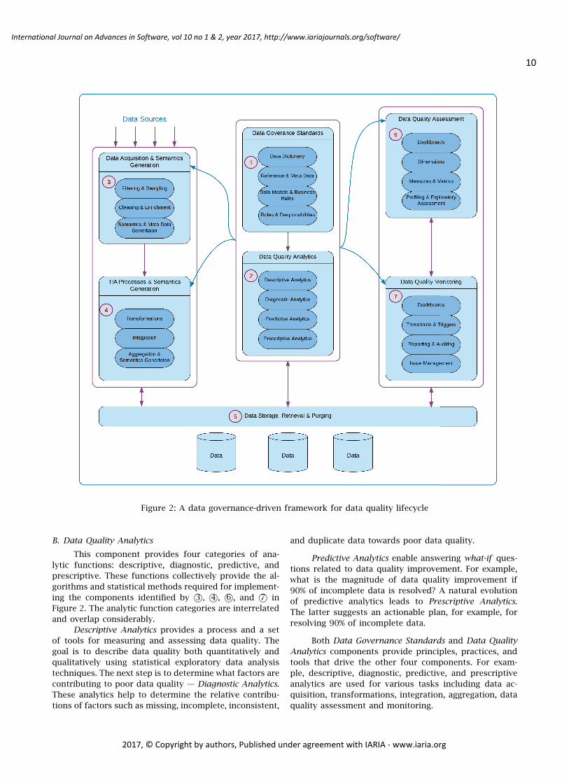
Figure 2: A data governance-driven framework for data quality lifecycle

B. Data Quality Analytics

This component provides four categories of ana-

lytic functions: descriptive, diagnostic, predictive, and

prescriptive. These functions collectively provide the al-

gorithms and statistical methods required for implement-

ing the components identified by 3©, 4©, 6©, and 7© in

Figure 2. The analytic function categories are interrelated

and overlap considerably.

Descriptive Analytics provides a process and a set

of tools for measuring and assessing data quality. The

goal is to describe data quality both quantitatively and

qualitatively using statistical exploratory data analysis

techniques. The next step is to determine what factors are

contributing to poor data quality — Diagnostic Analytics.

These analytics help to determine the relative contribu-

tions of factors such as missing, incomplete, inconsistent,

and duplicate data towards poor data quality.

Predictive Analytics enable answering what-if ques-

tions related to data quality improvement. For example,

what is the magnitude of data quality improvement if

90% of incomplete data is resolved? A natural evolution

of predictive analytics leads to Prescriptive Analytics.

The latter suggests an actionable plan, for example, for

resolving 90% of incomplete data.

Both Data Governance Standards and Data Quality

Analytics components provide principles, practices, and

tools that drive the other four components. For exam-

ple, descriptive, diagnostic, predictive, and prescriptive

analytics are used for various tasks including data ac-

quisition, transformations, integration, aggregation, data

quality assessment and monitoring.

10



C. Data Acquisition & Semantics Generation

This component is comprised of three processes:

Filtering & Sampling, Cleaning & Enrichment, and Se-

mantics & Meta Data Generation. Big data applications

typically acquire data from multiple sources. Some of this

is streaming data. To manage the complexities of velocity

and volume facets, streaming data is often sampled and

filtered. Data is sampled randomly for retention and

further processing. Also, the data is averaged over a

moving window and only the averaged data is retained.

Moreover, data may be filtered based on certain predi-

cates. For example, if the values fall within a predefined

range, such data is retained. Alternatively, data values

that fall outside a predefined range are retained. Such

data represents anomalies and outliers and is useful for

detecting unusual events.

The next process is Cleaning & Enrichment, which

primarily targets data standardization, detection and re-

moval of duplicates, inconsistent data resolution, impu-

tation for missing data, incomplete data strategies, and

matching data across multiple sources (aka data/record

linking). Cleaning & Enrichment process uses analytic

functions to automatically or semi-automatically accom-

plish the above tasks. A meta data by-product of cleaning

and enrichment is annotation, which is used to explain

the evolution of data.

Several pieces of additional information are cap-

tured during the data acquisition phase. In the case of IoT

devices, for instance, the types of sensors used, precision

and scale for data calibration, and sampling methods

employed is recorded. This meta data essentially cap-

tures semantics about the IoT data. These semantics and

meta data is essential to determining suitable statistical

analysis methods in downstream big data and machine

learning applications.

Data cleaning procedures employ a range of ad-

hoc data transformations. These transformations are rela-

tively simple compared to those described in Section VI-D.

An example of a simple cleaning procedure is the one that

normalizes data — when some observations are measured

in meters while others are measured in kilometers, all

measurements are converted either meters or kilometers.

Missing values can be automatically determined in some

cases, if the missing value in conjunction with other avail-

able values and associated constraints entail a unique

solution. Some quantitative approaches to data cleaning

are based on detecting outliers. As discussed in Section B,

detection of outliers is not a trivial task.

Imputation is a statistical technique for estimating

missing values. Though several imputation methods are

available, there is no imputation method that works in

all cases. An imputation model is selected based on the

availability of auxiliary information and whether or not

the data to be inputed is subject to multivariate edit

restrictions. A practical strategy is to impute missing

values without considering edit restrictions and then

apply minimal adjustments to the imputed values to

comply with edit restrictions.

There are three basic numeric imputation models:

imputation of the mean, ratio imputation, and general-

ized linear regression model. In the imputation of the

mean model, imputation value is the mean computed over

the observed values. The usability of this model is limited

since it causes a bias in measures of spread, which are

estimated from the sample after imputation.

In the ratio imputation model, the imputation value

of variable xi is computed as the product of R̂yi, where

yi is a covariate of xi and R̂ is an estimate of the average

ratio between x and y . R̂ is computed as the ratio of the

sum of observed x values to the sum of corresponding y

values. Lastly, in the generalized linear regression model,

the missing value x̂i is imputed as:

x̂i = β̂0 + β̂1y1,i + β̂2y2,i + · · · + β̂kyk,i

where β̂0, β̂1, . . . , β̂k are estimated linear regression coef-

ficients of the auxiliary variables y1, y2, . . . , yk.

In another method called hot deck imputation, miss-

ing values are imputed by copying values from similar

records in the same dataset. This imputation method is

applicable to both numerical and categorical data. The

main consideration in the hot deck imputation method is

determining which one of the observed values be chosen

for imputation. This leads to the following variations:

random hot-deck imputation, sequential hot deck impu-

tation, and predictive mean matching. Others include k

nearest neighbor imputation and an array of methods for

imputation of missing longitudinal data [43]. Imputation

results in datasets with very different distributional char-

acteristics compared to the original dataset [44].

D. TIA Processes & Semantics Generation

Transformation, Integration, Aggregation (TIA) &

Semantics Generation are the four processes that underlie

this component. Many statistical procedures assume data

normality and equality of variance. Data is transformed

for improving data normality and equalizing variance.

Such data transformations include inversion and reflec-

tion, conversion to a logarithmic scale, and square root

and trigonometric transforms. It should be noted that

these transformations are more complex than the ones

discussed in Section VI-C, and use sophisticated rule-

based approaches.

Large organizations typically have very complex

data environments comprised of several data sources.

This entails the need for integrating and aggregating data

from these sources. Integration requires accurately iden-

tifying the data associated with an entity originating from

multiple sources. However, not all data source providers

use the same identification schemes consistently. Several

tools are available for data integration such as the Talend

Open Studio and Pentaho Data Integration. Once the

data is integrated, aggregates are precomputed to speed

up the analysis tasks. Transformation, integration, and

11



aggregation processes generate substantial meta data as

well as semantics, which are also captured and stored.

E. Data Storage, Retrieval & Purging

This component provides persistent storage, query

mechanisms, and management functionality to secure

and retrieve data. Both relational and NoSQL database

systems are used to realize this functionality [36]. Sev-

eral data models and query languages are provided to

efficiently store and query structured, semi-structured,

and unstructured data [35]. Rules-driven processing is

employed to purge expired and stale data.

F. Data Quality Measurement and Assessment

This component provides four primary functions:

dashboard view of current data quality, definition of data

quality dimensions and associated measures & metrics

to quantify dimensions, tools for measuring data quality

through exploratory profiling. Data quality assessment is

the process of evaluating data quality to identify errors

and discern their implications. The assessment is made

in the context of an intended use and suitability of data

for that use is evaluated.

Dashboards are graphical depictions of data quality

along and across the dimensions. Recall that data quality

dimensions and their assessment at a conceptual level are

discussed in Section V. Measures and metrics are used to

quantify data quality dimensions. Measures are intended

to quantify more concrete and objective attributes such

as the number of missing values. In contrast, metrics

quantify abstract, higher-level, and subjective attributes

such as data accuracy.

There are four measurement scales: nominal, ordi-

nal, interval, and ratio. The measurement scale deter-

mines which statistical methods are suitable for data

analysis. The nominal scale is the most basic and provides

just a set of labels for measurement. There is no inherent

ordering to the labels. For example, gender is measured

on a nominal scale comprised of two labels: male and

female. The ordinal scale is a nominal scale when ordering

is imposed on the labels. For instance, the Mohs scale

of mineral hardness is a good example of ordinal scale.

Mohs hardness varies from 1 to 10, where 1 corresponds

to talc and 10 to diamond. However, the scale is not

uniform. For instance, the diamond’s hardness is 10 and

the corundum’s is 9, but the diamond is 4 times harder

than the corundum.

In contrast with the ordinal scale, the interval scale

has equal distance between the values. However, the scale

does not have an inherent zero. For instance, a tem-

perature is measured using an interval scale in weather

prediction applications. However, 0 degrees Fahrenheit

does not represent the complete absence of temperature.

It does not make sense to add values on an interval scale,

but the difference between two values is meaningful. It

should be noted that 0 on the Kelvin scale is absolute zero

— complete absence of temperature. Finally, a ratio scale

is an interval scale with an inherent zero. The ratio of

two values on the ratio scale is meaningful. For instance,

10 degrees Kelvin is twice as hot as 10 degrees Kelvin.

As another example, money is measured on a ratio scale.

Data profiling is an exploratory approach to data

quality analysis. Statistical approaches are used to reveal

data usage patterns as well as patterns in the data [27],

[30]. Several tools exist for data quality assessment using

data profiling and exploratory data analysis. Such tools

include Tableau [45] and Talend Open Studio [46]. Other

tools are listed in Section VIII.

G. Data Quality Monitoring

This unit builds on the Data Quality Assessment

component’s functionality. Its primary function is to con-

tinually monitor data quality and report results through

dashboards and alerts. Data quality is impacted by pro-

cesses that acquire data from the outside world through

batch and real-time feeds. For example, an organization

may procure data feeds from multiple vendors. Issues

arise when different values are reported for the same data

item. For instance, financial services companies obtain

real-time price information from multiple vendors. If the

timestamped price for a financial instrument received

from vendors differ, how does the system select one of

the values as the correct price? Vendor source hierarchy is

an approach to solving this problem. It requires imposing

an ordering on the vendors based on their reputation. If

multiple prices are available for an instrument, select the

price from that vendor who has the highest reputation.

An approach to improving data quality using the conflict-

ing data values about the same object originating from

multiple sources is presented in [47].

Corporate mergers and acquisitions also contribute

to data quality degradation. These actions entail changes

to, for example, the identifiers of financial instruments.

The changes will make their way into data vendor feeds.

Automated real-time and batch feed ingestion systems

will record price information under the new identifiers,

effectively causing data quality decay by not recognizing

the relationship between the old and new identifiers.

Streaming data feeds as well as high volume batch feeds

require automated and real-time processing. Whether or

not to accept a data record must be determined on the

fly. If a data record is accepted whose data quality is

suspect, such information is recorded as meta data to

help data quality monitoring processes. User interfaces

also contribute to data quality decay. Irrespective of

data availability, users are forced to enter values for the

required fields on a form.

Another source of data quality degradation is when

systems are merged or upgraded. The systems being

merged may be operating under different sets of busi-

ness rules and user interfaces. The data may also over-

lap between the systems. Even worse, the overlapping

data may be contradictory. Systems merging typically

requires substantial manual effort and decisions made in

12



resolving data issues must be documented in the form

of meta data. Lastly, transformations, integration, and

aggregation also contribute to data quality decay. These

processes may entail loss of data precision and scale, and

replacement of old identifiers with new ones.

VII. A Reference Architecture for Implementing the

Data Governance-driven Framework for Data

Quality Life Cycle

Shown in Figure 3 is a reference architecture for

implementing the data governance-driven lifecycle frame-

work of Figure 2. The bottom layer persistently stores all

types of data managed by relational and NoSQL systems.

In addition to application data, business rules, reference

and master data, and meta data are also stored. The

next layer above is the hardware layer powered by both

conventional CPUs as well as the processors specifically

designed for machine learning tasks such as the neuro-

morphic chips.

The Parallel and Distributed Computing layer pro-

vides software abstractions, database engines, and open

source libraries to provide performance at scale required

in big data and machine learning environments. The im-

mediate layer above is dedicated for functionality needed

for four types of data analytics – descriptive, diagnostic,

predictive, and prescriptive. Various machine learning

algorithms comprise the underlying basis for achieving

the data analytics functions.

The data access layer is responsible for enforcing

the data governance-driven approach to implementing

data quality. It has a rules engine to execute and mange

business rules. This layer also controls encryption, se-

curity, privacy, compression, and provenance aspects of

the data. The layer above the data access layer primarily

provides authorization and access control features. It also

features privileged functions for system administrators.

The architecture specifies various types of query APIs

for applications, interactive users, and system adminis-

trators. The entire architecture can be implemented with

Free and Open Source Software (FOSS).

VIII. Tools for Data Quality Management

Given the data volumes and the tedious and error-

prone nature of the data quality tasks, tools are essential

for cleaning, transforming, integrating, and aggregating

data and to asses and monitor data quality. The following

taxonomy for data quality tools is for exposition purpose

only. However, it is difficult to demarcate functions based

on this taxonomy in open-source and commercial data

quality tools.

The first category of tools provide functions to

support descriptive analytics. These tools in the field are

referred to as data profiling or data analysis tools. They

primarily target column data in relational database tables,

and column data across tables. They help to identify

integrity constraint violations. It should be noted that

integrity constraints go beyond what can be declaratively

specified in relational databases. Complex integrity con-

straints can be specified in the form of business rules.

Another category of tools provides functions for

diagnostic analytics. For instance, if there is an integrity

constraint violation, these tools help to discover the root

cause of these violations. The third category of tools

focuses on how to fix the problems revealed by diagnostic

analytics. Data cleaning, integration, and transformation

tools come under this category. This functionality is pro-

vided by prescriptive analytics tools. The fourth category

of tools help to explore what if scenarios and perform

change impact analysis – what is the impact of changing a

value on overall data quality or on a specific data quality

dimension?

Historically, data cleaning tools performed mostly

name and address validation. The expanded functionality

in the current generation tools include standardization

of fields (e.g., canonical representation for date values),

validating values using regular expressions, parsing and

information extraction, rule-based data transformations,

linking related data, merging and consolidating data from

multiple sources, and elimination of duplicates. Some

tools go even farther and help to fix missing data through

statistical imputation. However, data quality tools do not

address the data accuracy dimension. This is typically

a manual process which requires significant human in-

volvement. A similar situation exists for data quality

monitoring. Data cleaning tool vendors are beginning

to address this need through audit logs and automated

alerts.

Profiler is a proof-of-concept, visual analysis tool

for assessing quality issues in tabular data [48]. Using

data mining methods, it automatically flags data that

lacks quality. It also suggests coordinated summary vi-

sualizations for assessing the quality of data in context.

Some of the leading software vendors for data quality

tools include Informatica, IBM, Talend, SAS, SAP, Trillium

Software, Oracle, and Information Builders.

Informatica offers three data quality products: In-

formatica Data Quality, Informatica Data as a Service, and

Data Preparation (Rev). IBM offers InfoSphere Information

Server for Data Quality, which also integrates data gover-

nance functionality. Trillium Software markets Trillium

RefineTM and Trillium PrepareTM. Trillium RefineTM is

used for data standardization, data matching, and data

enrichment through annotations and meta data. In con-

trast, Trillium PrepareTM focuses on data integration from

diverse sources through automated workflows and built-

in logic, which obviates the need for any programming.

Only Trillium Software offers data quality tools under

Software as a Service (SaaS) model. Talend provides an

array of products for data quality (end-to-end profiling

and monitoring), data integration, master data manage-

ment, and big data processing through NoSQL databases,

Apache Hadoop and Spark [46]. In addition to commer-

cially licensed software, Talend offers an open source

community edition with limited functionality.

13



Figure 3: A reference architecture for implementing the data quality lifecycle framework for big data and machine

learning

IX. Recommended Practices and Future Trends

Data quality has been an active area of research for

over four decades [49]. The progress has been hampered

by the domain-specific considerations and attendant nar-

rowly focused solutions. Solutions to simple problems

such as recognizing customers as they interact through

a wider range of channels and developing a single cus-

tomer view remains elusive even today. It is common

for organizations to have 50 or more customer contact

databases. Incomplete and missing data, inaccurate data,

dated data, and duplicate data are the most common data

quality problems. Exponential growth in data generation

coupled with social and mobile channels exacerbate the

data quality problem.

Integrity Constraints (ICs) do not prevent bad data.

ICs are only one step of a multi-step process for ensuring

data quality. Requiring a field to be non-empty in a user

interface is not sufficient to ensure that a user provides

a meaningful value. Furthermore, constraining a field to

a valid range of numerical values does not assure that

the values chosen are necessarily accurate. Constraint

enforcement through user interfaces often leads to user

frustration. In manually generated data contexts, if data

entry operators are forced to provide values, they may en-

ter incomplete and inaccurate values. In many cases, they

lack the domain knowledge to provide the correct data

especially in time-constrained transaction environments.

Advances in natural language understanding, language

modeling, and named entity recognition will help to

alleviate this problem [50].

Current generation user interfaces are designed to

accept or reject data values. An accepted value implies

complete confidence in its correctness. Instead, the inter-

face should enable specifying a degree of confidence in

addition to the value itself. It should be possible to edit

the data items with low confidence score at a later time

to increase their confidence score. Provenance tracking

should be tightly integrated with this method. Further-

more, statistical machine learning methods should be

leveraged to suggest appropriate data values. For ex-

ample, they can suggest values based on an underlying

statistical model of data distribution.

Annotation should be an integral part of data

quality tools. Annotating unusual or incomplete data is

invaluable for data cleaning, integration, and aggrega-

tion processes. Annotation makes it easier to identify

suspect data that needs correction. Though automated

approaches to outlier detection are highly desirable, cur-

rently outlier detection and treatment is a manual pro-

cess. In the short- to medium-term, approaches used in

visual analytics [51] should be brought to bear in outlier

detection. This approach helps to transition a completely

14



manual process to a semi-automated process. In visual

analytics, analysts use their domain knowledge and judg-

ment to validate information provided by algorithms.

Both Big Data Analytics and Data Science as new

academic disciplines will accelerate data quality research.

Furthermore, big data-driven machine learning [52] is

expected yield solutions that will achieve automatic do-

main adaptation through supervised and unsupervised

learning. Privacy-preserving data quality assessment will

gain importance to protect the privacy risks of various

stakeholders [53]. As the number of data sources in-

creases, the complexity of the transformations required

to integrate these data is surging. Data quality errors are

often spotted in the transformed data. New algorithms

are needed to identify the original data elements and their

sources corresponding to these errors [54].

X. Conclusions

The advent of big data and attendant renaissance

in machine learning offers both opportunities for and

challenges to data quality research. The true cost of fixing

a software bug goes up based on how far down the

software development lifecycle the bug is found. The IBM

Systems Science Institute reports that the cost of fixing a

bug that is discovered after the product has been released

is four to five times as the one discovered during design,

and up to 100 times more than the one discovered during

the maintenance phase. A similar scenario is generally

true for the costs associated with fixing problems caused

by poor data quality.

Historically, data quality tasks were manually car-

ried out with rudimentary support from data quality

tools. Manual and even semi-automated approaches are

impractical in the big data context. On the positive side,

machine learning and other advances in computer sci-

ence offer unprecedented opportunities to automate data

cleaning, assessment and monitoring tasks.

Until recently, data quality research has primarily

focused on structured data stored in relational databases

and file systems. The recent emergence of NoSQL systems

for big data management renders much of the traditional

data quality research inadequate and less relevant. In this

paper, we described a data governance-driven framework

for data quality lifecycle and a reference architecture

for implementing the framework. Our next step is to

implement the architecture shown in Figure 3 using open

source tools and libraries. We expect the application of

the resulting system on big data scale datasets to reveal

both the strengths and weaknesses of our proposed

architecture.

Appendix A

Machine Learning Systems

The facets of a machine learning systems include (1)

a representation (aka model) for the system, (2) methods

and data used for training the system, (3) convergence

and instability issues associated with the datasets and

training methods, (4) evaluation of the effectiveness of

the system using test data, and (5) model selection -

searching for the best model in the model space. We

use the terms machine learning algorithm and model

synonymously.

Input to machine learning algorithms is usually

represented as n− dimensional (feature) vectors. Each

component in the vector corresponds to a (predictor)

variable value (aka feature). All input vectors are of

the same dimension. The output of a machine learning

algorithm can be a scalar or a vector. The dimensions

of this response vector and the input vectors need not

be the same. A labeled input instance refers to both the

feature vector and the expected result.

A. Prediction and Clustering

Broadly speaking, there are two major classes of

machine learning algorithms: prediction and clustering.

Prediction problems involve predicting an outcome for a

given input. For example, given an email, predict its class:

spam or not spam. Other examples include predicting

whether a credit card transaction is a fraud, whether

or not to approve an application for bank credit, and

predicting credit scores of consumers.

Regression and classification are both prediction

problems. Regression predicts a value from a continu-

ous set, for example, predicting the credit score of a

consumer, which is a real number. Classification, on the

other hand, classifies an input to one of the predefined

classes. For instance, classifying hand-written digits into

one of the ten classes, where each class corresponds

to a decimal digit. Both regression and clustering use

supervised learning.

Clustering refers to another class of machine learn-

ing algorithms. Their primary function is to organize a set

of objects into two or more classes in a way that the ob-

jects in a class are maximally similar to each other, while

maximally different from the objects in other classes.

Examples of clustering include categorizing students in a

class based on their predominant learning style, classify-

ing customers into groups to enable targeted marketing

for new products and services, and identifying clusters

of functionally related genes.

B. Supervised, Semi-supervised, and Unsupervised Learn-

ing

Supervised, semi-supervised, and unsupervised are

the three major approaches to training machine learning

algorithms. In supervised learning, an algorithm learns

from the training data, which is provided in the form

of labeled instances. The result of learning is a model

such as a decision tree or an artificial neural network. The

model is used to predict a response when it is presented

with input data which is not seen before by the model.

For supervised learning algorithms, one typically needs to

choose values for the model parameters. For instance, the

number of trees is one of the model parameters for the

15



random forest models. Model parameters are determined

using experimentation and hyperparameter tuning.

In unsupervised learning, an algorithm learns on

its own using the supplied data. Often, unsupervised

algorithms are used to automatically generate labeled

instances, which are then used in supervised learning.

Semi-supervised learning is a hybrid of supervised and

unsupervised learning. It makes use of mostly unlabeled

data for training. In other words, the training data is

comprised of a small amount of labeled data and a large

amount of unlabeled data.

C. Parametric and Non-parametric Learning

Parametric vs. non-parametric is another way to

classify machine learning algorithms [55]. Parametric al-

gorithms employ a known functional form such as a

linear function to map input (feature) vectors to re-

sponse vectors. The chosen functional form determines

the number of parameters of the model. For example, for

the linear regression model, the model parameters are

intercept and slope. The model parameters are learned

from the training data. Perceptron and linear discriminant

analysis are two other examples of parametric learning al-

gorithms. Non-parametric algorithms, on the other hand,

do not assume a functional form a priori. Using the

training data, these algorithms learn functional forms

and their parameters. Non-parametric algorithms require

large training datasets. Examples of such algorithms are

k− nearest neighbors (kNN), support vector machines,

artificial neural networks, and naive Bayes classifiers.

D. Linear and Nonlinear Learning Algorithms

Linear vs. nonlinear is yet another way to classify

machine learning algorithms. As the name implies, linear

machine learning algorithms typically employ a linear

function to map input vectors to response vectors. Linear

algorithms include gradient descent optimization, linear

regression, logistic regression, and linear discriminant

analysis. Nonlinear machine learning algorithms include

classification and regression trees (CART), naive Bayes,

kNN , learning vector quantization (an extension of kNN),

and support vector machines.

E. Ensemble Machine Learning, Bagging, and Random

Forests

Variations on the algorithms discussed above in-

clude ensemble learning, bagging, and random forest.

An ensemble algorithm combines the predictions from

multiple machine learning algorithms to make a more

accurate prediction than any individual model. Bootstrap

aggregation (aka bagging) is an ensemble learning algo-

rithm. It is a general procedure to reduce variance for

high variance algorithms such as the Classification and

Regression Tree (CART). First, we create many random

subsamples of the training dataset with replacement.

Second, using each subsample, we train a CART model.

Given a new input instance, it is classified using each of

the CART models. The input belongs that class which is

arrived at by the majority of the CART models.

Even with bootstrap aggregation/bagging, CART

trees may posses significant structural similarities, which

results in high correlation in their predictions. This is

due to the fact that a strong predictor typically gets

included in almost all trees. This makes the trees cor-

related and thus their predictions are also correlated.

Ensemble methods work better if the predictions from

the underlying individual models are either uncorrelated

or weakly correlated.

Boosting (aka boosted tree) overcomes the corre-

lated predictions problem by creating a strong model

from a number of weak models. It first creates a model

from the training data. A second model is then created,

whose goal is to correct the shortcomings in the first

model. This process is continued until the ensemble

correctly predicts the training dataset or a pre-specified

number of models have been added. AdaBoost is the first

successful boosting algorithm for binary classification

problems. It can also be used to boost the performance

of any machine learning algorithm. AdaBoost makes a

prediction based on the weighted average of the weak

classifiers.

Random Forests approach overcomes the correlation

between trees problem in bagged trees by de-correlating

the trees. As in bagging, a number of trees on boot-

strapped training data are developed. However, each time

a split in a tree is considered, only a random sample of a

subset of predictors is allowed for the split to be based

upon.

F. Evaluating Prediction Accuracy

For regression prediction problems (e.g., linear and

nonlinear models) evaluation measures include R2, ad-

justed R2, Akaike Information Criteria (AIC), Bayesian

Information Criteria (BIC), and Mallow’s Cp.

Machine learning algorithms for binary classifica-

tion prediction problems are evaluated using the con-

fusion matrix shown in Table II. Consider the problem

of predicting flight delays. This is a binary classifica-

tion problem — given an input vector, which represents

variables (e.g., origin airport, destination airport, flight

number, month, day of the month, day of the week,

actual departure time, scheduled departure time, actual

arrival time, and scheduled arrival time), the classifier will

predict whether or not the flight will be delayed (a yes/no

response).

Consider the table cell labeled “True Positive (TP).”

The value in this cell indicates the number of times the

model predicted delays correctly – the model predicted

flight delay and the flight was actually delayed. A bigger

value is better for this case. The value in the cell labeled

“False Positive (FP)” indicates the number times the model

predicted delays when actually there were no delays.

Smaller values are desired for this case. Next, the value

16



TABLE II: Structure of a confusion matrix

Predicted Value

Positive Negative Row Total

Actual ValuePositive True Positive (TP) False Negative (FN) P ′

Negative False Positive (FP) True Negative (TN) N′

Column Total P N

in cell labeled “False Negative (FN)” indicates the number

of times the model did not predict delays when there

were delays. A smaller value for this case is preferred.

Lastly, the value in the cell labeled “True Negative (TN)”

indicates the number of times the model did not predict

delays when there were no delays. Here again, a bigger

value is better.

Let P = TP + FP and N = FN + TN . Four metrics

are defined — PPV, TPR, ACC, and F1 score — as shown

in Table III. Which metric is relevant depends on the

problem being addressed. In the case of the airline delay

prediction problem, accuracy is a more relevant metric.

For multi-class classification prediction problems

(e.g., classification trees), classification error rate is used

as the evaluation metric. The latter measures the fraction

of the training observations in a region that do not belong

to the most common class. Other measures include the

Gini index, which measures the total variance across all

the classes. An alternative to the Gini index is cross-

entropy. Gini index and cross-entropy are quite similar

numerically.

Appendix B

Outliers

Extreme values in the data are not necessarily out-

liers. For instance, for a univariate case, a perfect SAT

score from a rural high school in the United States is an

extreme value, but not an outlier. For a multivariate case,

a similar example is a student from a rural background

pursuing a Ph.D. degree at a prestigious university. Errors

in data acquisition processes and recording contribute to

extreme values.

We first define some terminology to facilitate dis-

cussion about outlier detection. Univariate context in-

volves only one input variable, whereas the multivariate

context refers to the presence of more than one input

variable. In statistics, the terms statistic and estimator

are related but are distinct concepts. A statistic relates

to a sample. For example, sample mean is a statistic. An

estimator also relates to a sample, but in the context of an

unknown property of a statistical model. An estimator is

a rule for estimating the unknown property of the model.

Both location equivariance and scale equivariance

are important properties for all statistical measures of

location. Location equivariance refers to the fact that if a

constant is added to each data point in the dataset, the

measure of location will be increased by that constant

value. Likewise, scale equivariance corresponds to multi-

plication by a constant — when each point in the dataset

is multiplied by a constant results in a change in the

measure of location by the same constant. For multivari-

ate data, properties for measures of location are referred

to as affine equivariance. The latter extends the notion

of equivariance beyond location and scale to measures of

multivariate dispersion. For example, covariance matrices

are affine equivariant, but are not robust in the presence

of outliers.

A. Implications of Outliers

Outliers can have a dramatic impact on the per-

formance of machine learning algorithms and statistical

procedures including clustering and factor analysis [44].

Clustering is especially sensitive to outliers. Outliers

can also distort Pearson’s correlation coefficient, pose

difficulties in regression analysis, and erroneously imply

collinearity among the input (aka predictor) variables.

Correlation coefficients based methods such as factor

analysis and structural equation modeling are negatively

impacted by the outliers.

B. Outlier Detection

A commonly used approach tags a data point as an

outlier, if its value is more than two or three standard

deviations from the mean. This approach may actually

mask an outlier since outliers can inflate the standard

deviation. For unimodal and symmetrically distributed

data, the box-and-whisker plot method is a popular ap-

proach for outlier detection. For skewed distributions,

data is first transformed using a logarithmic or square

root function. Other methods such as the one proposed

by Hiridoglou & Berthelot [56] for positive observations,

take the skewness into consideration.

Approaches to multivariate outlier detection must

maintain affine equivariance. A commonly recommended

approach for multivariate outlier detection is the Maha-

lanobis distance (D2). Other methods include Minimum

Volume Ellipsoid (MVE), Minimum Covariance Determi-

nant (MCD), Fast MCD, and Minimum Generalized Vari-

ance (MGV) [44].

17



TABLE III: Evaluation measures based on confusion matrix

Evaluation Metric Name Computing the Metric

Precision or positive predictive value (PPV)TP

TP+FP

Recall (sensitivity or true positive rate (TPR))TP

TP+FN

Accuracy (ACC)TP+TNP+N

F1 score (harmonic mean of precision and sensitivity)2·TP

2·TP+FP+FN

Appendix C

Robust Statistics

Robust statistics are statistical methods that are

not significantly affected by outliers [57]. They provide

good performance for data coming from a wide range of

probability distributions, especially for data that is not

normally distributed. Modern robust statistical methods

offer considerably higher statistical power and a greater

understanding of data drawn from different probability

distributions [58].

A trimmed mean is the mean computed by exclud-

ing a certain percent of the largest and the same percent

of the smallest values from a dataset. For example, the

10% trimmed mean is the mean computed by excluding

10% percent of the largest and 10% percent of the smallest

values from the dataset. The trimmed mean calculation

requires first sorting the data points from the smallest

to the largest. The trimmed mean shields the influence

of data points at both ends that may unfairly affect the

traditional mean.

A related concept is Winsorizing data. Instead of

removing the 10% of the smallest values, they are set

equal to the smallest value that is not trimmed. Likewise,

10% of the largest values are set equal to the largest value

that is not trimmed. In other words, 10% of the smallest

values are set equal to the value corresponding to the

10th percentile, while the 10% of the largest values are set

equal to the value corresponding to the 90th percentile.

A simple robust analog of the Pearson’s correlation is the

Winsorized correlation. For example, a 90% Winsorized

correlation is calculated using the standard correlation

formula after trimming 5% of the smallest and 5% of the

largest values.

The notion of breakdown point is a key consid-

eration in assessing the impact of outliers. When the

proportion of corrupted data points in a dataset exceeds

a threshold called the breakdown point of an estimator,

the estimator can produce arbitrarily erroneous results.

There are two types of breakdown points: finite sample

breakdown point, and asymptotic breakdown point. The

finite sample breakdown point of an estimator is the

proportion of data that can be given arbitrary values

without affecting the estimator’s validity. Consider the

calculation of mean of the sample {x1, x2, x3, . . . , xn}.

Making any one of the values in the sample arbitrarily

large renders the sample mean invalid — a single bad

value causes the sample mean breakdown.

The finite sample breakdown point is necessarily

associated with the sample size n. In contrast, the asymp-

totic breakdown point is a single number, which is the

limit of the finite sample breakdown point as n goes to

infinity. For the sample mean, the finite sample break-

down point is1n , and the asymptotic breakdown point is

zero. In contrast, for the sample median, the finite sample

breakdown point is ⌊n−12n ⌋, and the asymptotic breakdown

point is one-half. If a statistic has a breakdown point of

0.2, then 20% of the data points in the dataset could be

outliers without markedly impacting the statistic. Median

and trimmed mean are examples of statistics with higher

breakdown points. However, they are less accurate in

estimating model parameters.

Appendix D

Dimensionality Reduction

The k− nearest neighbor (kNN) algorithm is a non-

parametric method used for both classification and re-

gression. When kNN is used for classification, the output

is the name of the class to which the object represented

by the input vector belongs. The class assigned to the

object is that class which is the most common among its

k nearest neighbors. In kNN based regression, the output

is the property value for the object represented by the

input vector, which is the average of the property values

of its k nearest neighbors. For instance, a credit score

of a new customer is the average of the credit scores

of the k nearest or similar customers. If the variables

come from skewed distributions, the effectiveness of the

majority voting based classification of kNN is diminished.

Instances of a more frequent class tend to dominate the

class prediction as these instances tend to be common

among the k nearest neighbors due to their sheer number.

The kNN algorithm requires a distance metric to

determine the k nearest neighbors of a given object.

Distance metrics used by the kNN include the Euclidean,

Hamming, Manhattan, Mahalanobis, and Minkowski. Eu-

clidean distance is a good measure for cases where the

input variables are similar in type. In contrast, Manhat-

tan distance is more appropriate for cases where the

18



input variables are dissimilar in type as in age, height,

weight, and gender. Distances between vectors are non-

computable if the component values are missing in the

input vectors.

A. Dimensionality Reduction through Variable Selection

Other names for the variable selection include fea-

ture selection, attribute selection, and variable subset se-

lection. Subspace learning (aka feature transformation) is

another approach to dimensionality reduction. It is based

on the premise that a combination of the original features

may be more useful for machine learning. Subspace

learning transforms the original features to a new feature

space, which has lower dimensionality.

Fisher criterion plays an important role in dimen-

sionality reduction for classification problems. It seeks a

feature representation which minimizes the within-class

distance while maximizing the between-class distance.

Fisher score is a feature selection method based on the

Fisher criterion. Linear Discriminant Analysis (LDA) is a

supervised subspace learning method based on the Fisher

criterion.

B. Principal Component Analysis and Exploratory Factor

Analysis

Principal Component Analysis (PCA) is another tech-

nique for feature selection. It is effective in situations

where the variables are highly correlated. The PCA op-

erates under the premise that the manifested/observed

and measured variables are of interest rather than the

unmanifested latent constructs in the dataset (which are

of interest in Exploratory Factor Analysis). PCA performs

analysis using all the variance in the (observed) variables,

without consideration for the underlying latent structure

of the variables. PCA reduces the number of (observed)

variables to a smaller number of principal components.

Each component is formed as a weighted linear combi-

nation of the variables. These components account for

most of the variance of the variables. Note that the total

amount of variance in PCA is equal to the number of

observed variables being analyzed.

The number of principal components extracted is

same as the number of observed variables. The first

principal component accounts for most of the variance

in the dataset, the second component accounts for the

second largest amount of variance, and so on. The first

few components that account for most of the variance are

retained, while the remaining components are discarded.

The principal components are uncorrelated with each

other. Instead of the original variables, the first few

principal components, for example, are used in linear

regression.

In contrast with PCA, Exploratory Factor Analysis

(EFA) enables exploring the underlying structure of a

dataset as well as serving as a general-purpose dimen-

sionality reduction technique. EFA and PCA are func-

tionally equivalent, but are different in how they ac-

complish their functions. EFA premises that there are

latent variables or factors in the dataset that give rise to

the observed variables. EFA employs a set of extraction

and rotation techniques, which are designed to model

the unobserved or latent constructs in the dataset. EFA

identifies the underlying factor structure for a set of

observed and measured variables. The user interactively

determines the number of factors to retain for analysis.

References

[1] V. Gudivada, D. Rao, and W. Grosky, “Data quality centric appli-cation framework for big data,” in Proceedings of the The SecondInternational Conference on Big Data, Small Data, Linked Dataand Open Data (ALLDATA 2016). Lisboa, Portugal: IARIA, Feb.2016, pp. 24 – 32.

[2] M. F. Bosu and S. G. MacDonell, “Data quality in empiricalsoftware engineering: A targeted review,” in Proceedings of the17th International Conference on Evaluation and Assessment inSoftware Engineering. New York, NY: ACM, 2013, pp. 171–176.

[3] Y. Shirai, W. Nichols, and M. Kasunic, “Initial evaluation of dataquality in a tsp software engineering project data repository,”in Proceedings of the 2014 International Conference on Softwareand System Process. New York, NY: ACM, 2014, pp. 25–29.

[4] M. Shepperd, “Data quality: Cinderella at the software metricsball?” in Proceedings of the 2nd International Workshop on Emerg-ing Trends in Software Metrics. New York, NY: ACM, 2011, pp.1–4.

[5] P. Phannachitta, A. Monden, J. Keung, and K. Matsumoto, “Caseconsistency: A necessary data quality property for software engi-neering data sets,” in Proceedings of the 19th International Con-ference on Evaluation and Assessment in Software Engineering.New York, NY: ACM, 2015, pp. 19:1–19:10.

[6] K. Sha and S. Zeadally, “Data quality challenges in cyber-physicalsystems,” J. Data and Information Quality, vol. 6, no. 2-3, pp.8:1–8:4, Jun. 2015.

[7] J. McNaull, J. C. Augusto, M. Mulvenna, and P. McCullagh, “Dataand information quality issues in ambient assisted living sys-tems,” J. Data and Information Quality, vol. 4, no. 1, pp. 4:1–4:15,Oct. 2012.

[8] S. A. Sheppard and L. Terveen, “Quality is a verb: The opera-tionalization of data quality in a citizen science community,”in Proceedings of the 7th International Symposium on Wikis andOpen Collaboration. New York, NY: ACM, 2011, pp. 29–38.

[9] L. Cao and H. Zhu, “Normal accidents: Data quality problemsin ERP-enabled manufacturing,” J. Data and Information Quality,vol. 4, no. 3, pp. 11:1–11:26, May 2013.

[10] H. Xu, “What are the most important factors for accounting infor-mation quality and their impact on ais data quality outcomes?” J.Data and Information Quality, vol. 5, no. 4, pp. 14:1–14:22, Mar.2015.

[11] O. Curé, “Improving the data quality of drug databases using con-ditional dependencies and ontologies,” J. Data and InformationQuality, vol. 4, no. 1, pp. 3:1–3:21, Oct. 2012.

[12] P. Barnaghi, M. Bermudez-Edo, and R. Tönjes, “Challenges forquality of data in smart cities,” J. Data and Information Quality,vol. 6, no. 2-3, pp. 6:1–6:4, Jun. 2015.

[13] A. Klein, “Incorporating quality aspects in sensor data streams,”in Proceedings of the ACM First Ph.D. Workshop in CIKM. NewYork, NY, USA: ACM, 2007, pp. 77–84.

[14] D. Kontokostas, P. Westphal, S. Auer, S. Hellmann, J. Lehmann,R. Cornelissen, and A. Zaveri, “Test-driven evaluation of linkeddata quality,” in Proceedings of the 23rd International Conferenceon World Wide Web. New York, NY: ACM, 2014, pp. 747–758.

[15] S. K. Bansal and S. Kagemann, “Integrating big data: A semanticextract-transform-load framework,” Computer, vol. 48, no. 3, pp.42–50, 2015.

[16] N. Martin, A. Poulovassilis, and J. Wang, “A methodology andarchitecture embedding quality assessment in data integration,”J. Data and Information Quality, vol. 4, no. 4, pp. 17:1–17:40, May2014.

[17] K.-S. Na, D.-K. Baik, and P.-K. Kim, “A practical approach formodeling the quality of multimedia data,” in Proceedings of theNinth ACM International Conference on Multimedia. New York,NY: ACM, 2001, pp. 516–518.

19



[18] A. Na’im, D. Crawl, M. Indrawan, I. Altintas, and S. Sun, “Mon-itoring data quality in kepler,” in Proceedings of the 19th ACMInternational Symposium on High Performance Distributed Com-puting. New York, NY: ACM, 2010, pp. 560–564.

[19] H. M. Sneed and R. Majnar, “A process for assessing data quality,”in Proceedings of the 8th International Workshop on SoftwareQuality. New York, NY: ACM, 2011, pp. 50–57.

[20] V. Gudivada, R. Baeza-Yates, and V. Raghavan, “Big data: Promisesand problems,” IEEE Computer, vol. 48, no. 3, pp. 20–23, Mar.2015.

[21] Y. Qin, Q. Z. Sheng, N. J. Falkner, S. Dustdar, H. Wang, and A. V.Vasilakos, “When things matter: A survey on data-centric internetof things,” Journal of Network and Computer Applications, vol. 64,pp. 137 – 153, 2016.

[22] Y. S. Abu-Mostafa, M. Magdon-Ismail, and H.-T. Lin, Learning FromData. AMLBook, 2012.

[23] C. Batini, C. Cappiello, C. Francalanci, and A. Maurino, “Method-ologies for data quality assessment and improvement,” ACMComput. Surv., vol. 41, no. 3, pp. 16:1–16:52, Jul. 2009.

[24] V. Ganti and A. D. Sarma, Data Cleaning: A Practical Perspective,ser. Synthesis Lectures on Data Management. Morgan & ClaypoolPublishers, 2013.

[25] D. Loshin, The Practitioner’s Guide to Data Quality Improvement.Burlington, Massachusetts: Morgan Kaufmann, 2010.

[26] TDWI. (2016) The data warehousing institute. Last visited: 14May 2017. [Online]. Available: https://tdwi.org/Home.aspx

[27] J. W. Osborne, Best practices in data cleaning: a complete guide toeverything you need to do before and after collecting your data.Thousand Oaks, CA: SAGE, 2013.

[28] D. McGilvray, Executing Data Quality Projects: Ten Steps to QualityData and Trusted Information. San Francisco, CA: MorganKaufmann Publishers Inc., 2008.

[29] D. Rao, V. N. Gudivada, and V. V. Raghavan, “Data quality issuesin big data,” in IEEE International Conference on Big Data (BigData). Santa Clara, California: IEEE Computer Society, Oct 2015,pp. 2654–2660.

[30] A. Maydanchik, Data quality assessment. Bradley Beach, NewJersey: Technics Publications, 2007.

[31] X. L. Dong, E. Gabrilovich, K. Murphy, V. Dang, W. Horn, C. Lu-garesi, S. Sun, and W. Zhang, “Knowledge-based trust: Estimatingthe trustworthiness of web sources,” Proc. VLDB Endow., vol. 8,no. 9, pp. 938–949, May 2015.

[32] X. Yin, J. Han, and P. S. Yu, “Truth discovery with multipleconflicting information providers on the web,” IEEE Transactionson Knowledge and Data Engineering, vol. 20, no. 6, pp. 796–808,jun 2008.

[33] J. Cheney, P. Buneman, and B. Ludäscher, “Report on the princi-ples of provenance workshop,” SIGMOD Rec., vol. 37, no. 1, pp.62–65, Mar. 2008.

[34] Y.-W. Cheah, “Quality, retrieval and analysis of provenance inlarge-scale data,” Ph.D. dissertation, Indianapolis, IN, 2014, in-diana University.

[35] V. N. Gudivada, D. Rao, and V. V. Raghavan, “NoSQL systems forbig data management,” in 2014 IEEE World Congress on Services.Los Alamitos, CA, USA: IEEE Computer Society, 2014, pp. 190–197.

[36] V. Gudivada, D. Rao, and V. Raghavan, “Renaissance in databasemanagement: Navigating the landscape of candidate systems,”IEEE Computer, vol. 49, no. 4, pp. 31 – 42, 2016.

[37] V. Gudivada, “Data analytics: Fundamentals,” in Data Analyticsfor Intelligent Transportation Systems, M. Chowdhury, A. Apon,and K. Dey, Eds. New York, NY: Elsevier, Apr. 2017, pp. 31 – 67,ISBN: 978-0-12-809715-1.

[38] C. Lehmann, K. Roy, and B. Winter. The state ofenterprise data quality: 2016. Last visited: 14 May2017. [Online]. Available: http://pages.blazent.com/rs/184-CZE-628/images/Blazent_State_of_DataQuality_2016.pdf

[39] P. D. Allison, Missing Data. SAGE Publications, 2001.

[40] S. Sarawagi, “Information extraction,” Foundations and TrendsDatabases, vol. 1, no. 3, pp. 261–377, Mar. 2008.

[41] K. Jung, K. I. Kim, and A. K. Jain, “Text informationextraction in images and video: a survey,” Pattern Recognition,vol. 37, no. 5, pp. 977 – 997, Jan. 2004. [Online]. Available:https://doi.org/10.1016/j.patcog.2003.10.012

[42] M. H. DeGroot and M. J. Schervish, Probability and Statistics,4th ed. Pearson, 2011.

[43] J. M. Engels and P. Diehr, “Imputation of missing longitudinaldata: a comparison of methods,” Journal of Clinical Epidemiology,vol. 56, pp. 968 – 976, 2003.

[44] H. Finch, “Distribution of variables by method of outlier detec-tion,” Frontiers in Psychology, vol. 3, pp. 1–12, 2012.

[45] Tableau Software. (2016) Tableau cloud analytics. Last visited:14 May 2017. [Online]. Available: http://www.tableau.com/

[46] Talend Software. (2016) Talend Open Studio. Last visited: 14May 2017. [Online]. Available: https://www.talend.com/

[47] H. Müller, J.-C. Freytag, and U. Leser, “Improving data quality bysource analysis,” J. Data and Information Quality, vol. 2, no. 4,pp. 15:1–15:38, Mar. 2012.

[48] S. Kandel, R. Parikh, A. Paepcke, J. M. Hellerstein, and J. Heer,“Profiler: Integrated statistical analysis and visualization for dataquality assessment,” in Proceedings of the International WorkingConference on Advanced Visual Interfaces. New York, NY, USA:ACM, 2012, pp. 547–554.

[49] S. Sadiq, N. K. Yeganeh, and M. Indulska, “20 years of data qualityresearch: Themes, trends and synergies,” in Proceedings of theTwenty-Second Australasian Database Conference - Volume 115.Darlinghurst, Australia: Australian Computer Society, Inc., 2011,pp. 153–162.

[50] J. R. Talburt, “Special issue on entity resolution overview: Thecriticality of entity resolution in data and information quality,”J. Data and Information Quality, vol. 4, no. 2, pp. 6:1–6:2, Mar.2013.

[51] S. Venna, R. Gottumukkala1, and V. Raghavan, “Visual ana-lytic decision-making environments for large-scale time-evolvinggraphs,” in Cognitive Computing: Theory and Applications, ser.Handbook of Statistics, V. Gudivada, V. Raghavan, V. Govindaraju,and C. R. Rao, Eds. New York, NY: Elsevier, Sep. 2016, vol. 35,pp. 81 – 115.

[52] V. Gudivada, D. Rao, and V. Raghavan, “Big data driven naturallanguage processing research and applications,” in Big DataAnalytics, V. Govindaraju, V. Raghavan, and C. R. Rao, Eds. NewYork, NY: Elsevier, 2015, pp. 203 – 238.

[53] J. Freudiger, S. Rane, A. E. Brito, and E. Uzun, “Privacy preservingdata quality assessment for high-fidelity data sharing,” in Pro-ceedings of the 2014 ACM Workshop on Information Sharing &Collaborative Security. New York, NY, USA: ACM, 2014, pp. 21–29.

[54] A. Chalamalla, I. F. Ilyas, M. Ouzzani, and P. Papotti, “Descriptiveand prescriptive data cleaning,” in Proceedings of the 2014 ACMSIGMOD International Conference on Management of Data, ser.SIGMOD ’14. New York, NY: ACM, 2014, pp. 445–456.

[55] T. Hastie, R. Tibshirani, and J. Friedman, The Elements of Sta-tistical Learning: Data Mining, Inference, and Prediction, 2nd ed.New York, NY: Springer, 2009.

[56] M. Hiridoglou and J.-M. Berthelot, “Statistical editing and imputa-tion for periodic business surveys,” Survey Methodology, vol. 12,no. 1, pp. 73–83, 1986.

[57] R. R. Wilcox, Introduction to robust estimation and hypothesistesting, 4th ed. Boston, MA: Academic Press, 2016.

[58] R. R. Wilcox and H. J. Keselman, “Modern regression methods thatcan substantially increase power and provide a more accurateunderstanding of associations,” European Journal of Personality,vol. 26, no. 3, pp. 165–174, 2012.

20



Documents

Data Quality Considerations for Big Data and Machine