NBER WORKING PAPER SERIES

WHO SOLD DURING THE CRASH OF 2008-9? EVIDENCE FROM TAX-RETURNDATA ON DAILY SALES OF STOCK

Jeffrey HoopesPatrick Langetieg

Stefan NagelDaniel ReckJoel SlemrodBryan Stuart

Working Paper 22209http://www.nber.org/papers/w22209

NATIONAL BUREAU OF ECONOMIC RESEARCH1050 Massachusetts Avenue

Cambridge, MA 02138April 2016

We thank John Friedman, Clemens Sialm, Andrei Shleifer, Chris Williams, Stefan Zeume, and participants at the University of Michigan Public Finance seminar, the 2015 National Tax Association meetings, the NBER Behavioral Finance Meeting, the US Treasury Office of Tax Analysis, and the University of North Carolina Annual Tax Symposium for helpful discussion and comments. We also thank John Guyton of the Research, Analysis, and Statistics Division of the Internal Revenue Service for help with using the IRS administrative data. The views expressed here are those of the authors alone, and do not necessarily reflect the views of the Internal Revenue Service or the National Bureau of Economic Research.

At least one co-author has disclosed a financial relationship of potential relevance for this research. Further information is available online at http://www.nber.org/papers/w22209.ack

NBER working papers are circulated for discussion and comment purposes. They have not been peer-reviewed or been subject to the review by the NBER Board of Directors that accompanies official NBER publications.

© 2016 by Jeffrey Hoopes, Patrick Langetieg, Stefan Nagel, Daniel Reck, Joel Slemrod, and Bryan Stuart. All rights reserved. Short sections of text, not to exceed two paragraphs, may be quoted without explicit permission provided that full credit, including © notice, is given to the source.

Who Sold During the Crash of 2008-9? Evidence from Tax-Return Data on Daily Sales ofStockJeffrey Hoopes, Patrick Langetieg, Stefan Nagel, Daniel Reck, Joel Slemrod, and Bryan StuartNBER Working Paper No. 22209April 2016JEL No. G01,G11,G12

ABSTRACT

We examine individual stock sales from 2008 to 2009 using population tax return data. The share of sales by the top 0.1 percent of income recipients and other top income groups rose sharply following the Lehman Brothers bankruptcy and remained elevated throughout the financial crisis. Sales by top income and older age groups were relatively more responsive to increased stock market volatility. Volatility-driven sales were not concentrated in any one sector, but mutual fund sales responded more strongly to increased volatility than stock sales. Additional analysis suggests that gross sales in tax return data are informative about unobserved net sales.

Jeffrey HoopesOhio State University448 Fisher Hall2100 Neil AvenueColumbus, OH 43210hoopes@fisher.osu.edu

Patrick LangetiegInternal Revenue ServicePatrick.T.Langetieg@irs.gov

Stefan NagelRoss School of Business andDepartment of EconomicsUniversity of Michigan701 Tappan StreetAnn Arbor, MI 48109and NBERstenagel@umich.edu

Daniel ReckUniversity of MichiganEconomics Department238 Lorch Hall, 611 Tappan StreetAnn Arbor, MI 48109-1220dreck@umich.edu

Joel SlemrodUniversity of Michigan Business School701 Tappan StreetRoom R5396Ann Arbor, MI 48109-1234and NBERjslemrod@umich.edu

Bryan StuartDepartment of EconomicsUniversity of Michigan611 Tappan St.Lorch HallAnn Arbor, MI 48109-1220bastuart@umich.edu

1

Introduction

Periods of turmoil in stock markets—such as September 2008 in the wake of the Lehman

Brothers bankruptcy—are associated with large declines in prices, abnormally high intra-day

price volatility, and high trading volume. Market commentary often characterizes these periods

as "sell-offs." As always, there is a buyer for every seller, so investors as a group cannot all be

sellers. What may be happening instead during these instances is that some investors sell out,

leaving the remaining investors to bear the risk of stock ownership. Such a reallocation of asset

ownership among heterogeneous investors is consistent with the high level of trading activity

observed during such periods. Little is known, however, about the characteristics of the investors

that are prone to sell in the midst of market turmoil. This paper uses administrative data from the

Internal Revenue Service, consisting of billions of third-party reports on all sales of stock in

United States taxable individual accounts, to understand which individuals sold stock during the

tumultuous market events of 2008 and 2009. Our main finding is that investors at the very top of

the income distribution—both the top 1 percent and even the top 0.1 percent—are, along with

older investors, much more likely to sell stock during times of market tumult than other

investors.

A number of factors can cause certain investors to be relatively sensitive to market

tumult. Some investors may be forced to sell due to constraints on their risk-bearing capacity

(e.g., leverage constraints, liquidity shocks), some may be less tolerant of short-run risk than the

average investor (e.g., close to retirement), some may perceive themselves to be better informed

than others and anticipate a further price decline, and some investors may lose trust in the stock

market altogether and perceive it as a rigged game. While some of these reasons for selling could

2

apply equally to both institutional and individual investors, others are primarily relevant for

individual investors (and the flows they direct in and out of institutional investment products).

Understanding heterogeneity in investors' propensity to sell sheds light on several key

questions in finance and macroeconomics, including the mechanisms that give rise to elevated

premia for bearing risk (Bollerslev and Todorov 2011; Martin 2015) and for providing liquidity

(Nagel 2012) following market tumult episodes. If part of the investor population has a tendency

to sell during times of market turmoil, this leaves a smaller set of investors holding aggregate

stock market risk. They must be enticed to do so by a higher risk premium and by greater

compensation for absorbing the liquidity demand of those who want to sell. Empirical evidence

on such episodic shifts in stock ownership has so far remained largely elusive due to lack of data.

In this paper, we study this set of questions with a unique new data set that allows us to

track, at a daily frequency, sales of stocks and mutual fund shares in the population of U.S.

taxable individual investors. The data are extracted from the universe of (anonymized) tax

returns filed with the Internal Revenue Service (IRS), and allow us to match asset sales reported

for capital gains taxation purposes with some demographic information on each taxpayer. While

we do not observe asset purchases in these tax records, we present indirect evidence from

dividend receipts and a supplementary brokerage account data set suggesting that individuals

with high levels of gross sales are also, to a substantial extent, net sellers of stocks.

We focus our analysis on 2008 and 2009, and further zoom in on the period immediately

following the bankruptcy of Lehman Brothers in September 2008. We find that, starting in

September 2008, the share of sales volume attributed to the top 0.1 percent of income recipients

rises sharply until the beginning of 2009. More generally, we find that high-income taxpayers

have a greater propensity to sell during periods of market tumult. In regression analysis, we

3

measure tumult with lagged one-day changes in the VIX index. The VIX index is a measure of

(risk-adjusted) expected market volatility and it is commonly used as a proxy for market tumult

and as a crisis indicator (see Adrian and Shin 2010; Longstaff 2010; Nagel 2012). Stock market

returns are typically negative on days when the VIX rises. We find that sales volume rises much

more strongly with lagged VIX changes for the top 95-99, 99-99.9, and 99.9-100 income

percentiles than for other income groups over the period 2008 to 2009. In multi-dimensional

analysis, both high income and age over 60 are associated with a strongly positive sales volume-

VIX relationship, as are income and receipt of Social Security income.

The greater sensitivity of older investors is consistent with the idea that investors close to

retirement (with less opportunity to make up losses through future labor income) should be

particularly sensitive to a perceived rise in risk (Chai et al. 2011). The tendency of high-income

investors to sell in high-volatility episodes could be a consequence of their tendency to pay

greater attention to their portfolios (Sicherman et al. 2016) and it could indicate that financially

more sophisticated investors perceive themselves better able to time the market.1 Another

possibility is that high-income investors are more likely to own stocks on margin. As a

consequence, a fall in asset prices or a rise in risk leads them to delever their portfolio by through

sales of risky assets (Kimball et al. 2011). A third potential explanation that could explain both

the age- and income-related findings is that selling during tumultuous periods interacts with the

disposition effect, i.e., the tendency of investors to avoid selling stocks with accumulated losses

(Shefrin and Statman 1985; Odean 1998). Prior evidence in Dhar and Zhu (2006) and Calvet,

Campbell, and Sodini (2009) indicates that the disposition effect is stronger for younger

investors and those with lower wealth. This reluctance to realize losses among the young and less

1 Recent work by Moreira and Muir (2016) suggests that temporarily reducing stock market exposure following

burst of high volatility may in fact be a utility-improving timing strategy.

4

wealthy could be the reason why their sales volume is less sensitive to market tumult.2 Other

demographic characteristics of investors—gender, marital status, region and state of residence,

presence and amount of a mortgage interest deduction, and 2007 zip-code-level house price

growth—are not related to the volatility sensitivity of stock sales.

We also analyze separately the sales volume of individual stocks and mutual funds.

Taxpayers’ mutual fund sales volume is more sensitive to changes in the VIX than is sales

volume of individual stocks. This also parallels findings for the disposition effect. Chang,

Solomon, and Westerfield (2016) show that the disposition effect is present for non-delegated

assets such as individual stocks, but not for delegated assets such as mutual funds. Thus, the

disposition effect could have a dampening effect on tumult-driven selling of individual stocks.

For delegated assets, Chang, Solomon, and Westerfield argue that cognitively dissonant investors

blame managers for stock market losses and withdraw their funds in response. A related notion is

that investors lose trust in financial intermediaries in response to market turmoil (Dorn and

Weber 2013). Although sales in financial stocks clearly respond to specific events, we find no

evidence that sales in finance responded more strongly to changes in the VIX than sales in most

other sectors.

The data we analyze are, in a number of ways, substantially better than the data sets that

have been studied up to now. Existing studies of investor responses to market movements and

changes in risk use data either from investor surveys (Guiso et al. 2013; Hudomiet et al. 2011;

Shiller 1987), from non-randomly selected samples of portfolio holdings data (Dorn and Weber

2013; Hoffmann et al. 2013; Weber et al. 2012; Barrot et al. 2016), administrative data from

Sweden that are available only at annual frequency (Calvet et al. 2009), or data on institutional

2 While the literature on the disposition effect focuses on the cross-section of individual stock trades, our results show that the findings in this literature may also be relevant for understanding individuals’ reaction to market tumult.

5

investor portfolios (see Ben-David, Franzoni, and Moussawi (2012); Cella et al. (2013) for the

crisis in 2008; see Brunnermeier and Nagel (2004); Griffin et al. (2011) for the Nasdaq crash in

2000). Our data let us investigate, for the first time, the population of U.S. taxable investors as a

whole at a daily frequency.

The data set is not perfect, though. The data set covers only reported taxable sales, but

not purchases of stocks and mutual funds. Additional analyses show, however, that there is a

strong relationship between gross selling, which we observe, and net selling (i.e., sales minus

purchases), which we do not observe. First, we examine data from a discount brokerage that

reports both gross and net sales (Barber and Odean 2000). We find a very strong positive

relationship between gross and net sales. Furthermore, net sales of brokerage customers rise with

changes in the VIX in similar ways as the gross sales of taxpayers in our data. Second, in the IRS

data, we examine changes in dividend income reported on individual tax returns. Here we find a

strong negative relationship between gross sales in a given year (e.g. 2008) and the change in

dividend income from the previous year (2007) to the subsequent year (2009). Despite coming

from different sources and time periods, the quantitative results from discount brokerage data

and from changes in dividend income on tax returns are highly consistent with one another,

suggesting that $1 of gross sales corresponds to about $0.33 in net sales.

Another shortcoming of the data set is that we do not observe sales in non-taxable

accounts, such as Individual Retirement Accounts. We analyze data from the 2007-2009 panel of

the Survey of Consumer Finance, which contains data on wealth in taxable and non-taxable

accounts, including pensions and trusts. We find that the share of wealth in taxable accounts is

relatively higher for individuals at the top of the income distribution, and for older individuals.

These facts rule out the concern that our main findings are driven by older and higher-income

6

people holding a disproportionately small share of their equities in taxable accounts.

Additionally, net sales in taxable accounts between the 2007 and 2009 waves of the survey are

strongly related to total net sales, suggesting that our analysis of sales in taxable accounts are

informative about total asset holdings.

Our study connects to a number of recent papers that have started to shed light on the

reaction of different types of investors to the market turmoil during the financial crisis. The

evidence from existing studies is mixed, possibly because samples used in these studies are small

and selective. Dorn and Weber (2013) find that customers of a large German retail bank kept

their overall equity allocations quite stable, but they withdrew from actively managed mutual

funds, which could be related to our finding that U.S. taxpayer mutual fund sales volume is more

sensitive to changes in VIX than stock sales are. Barrot et al. (2016) find that customers of a

French brokerage customers also withdrew from mutual funds, but they increased their exposure

to directly held stocks. Hoffmann et al. (2013) find that the brokerage customers in their sample

did not reduce the risk of their portfolios during the height of the crisis, even though,

temporarily, their risk tolerance dropped and they expected lower returns and higher risk. In

contrast, Weber et al. (2012) find substantial changes in risk taking associated with changes in

subjective perceptions of risk and return during this period in a survey of U.K. online brokerage

customers. Similarly, Guiso et al. (2013) find that both a qualitative and a quantitative survey-

based measure of risk aversion increased following the experience of the crisis, but they do not

find much predictable cross-sectional heterogeneity in the change in risk aversion. Although

certainly of interest, the small and selected nature of the samples in these studies limits the extent

to which one can learn about heterogeneity between demographic groups and how much one can

7

generalize from these findings. We turn now to describe the much more comprehensive data we

examine, our research design and its theoretical underpinning, and finally our results.

2. Data

This section describes the confidential administrative data and publicly available data we use,

and provides summary statistics and match rates across different data sources.

2.1 Tax Return Data

We use two types of tax-return data on U.S. individuals trading in taxable accounts. The

primary source of data is third-party information assembled by brokerages and provided to the

IRS and taxpayers on Form 1099-B.3 The raw data set contains all Form 1099-B’s for trades

occurring between January 1, 2000 and December 31, 2012. For any covered financial asset sold

in this period, Form 1099-B provides the sale price and date, the Committee on Uniform Security

Identification Procedures (CUSIP) number identifying the asset, an anonymized version of the

taxpayer identification number (TIN), which for an individual seller is a Social Security number,

along with several less relevant items.4

The second source of information we can link to asset sales is demographic information

from individual income tax returns (Forms 1040) and other records. These include, among other

details, age and gender (from Social Security records), number of dependents, whether the

individual takes a mortgage interest deduction, and the ZIP code of the filing address. We also

observe a variety of income measures, including wages and salaries, dividends, interest

payments, retirement benefits, and net income from self-employment, many of which are

supported by third-party information.

3 For a current year 1099-B, see www.irs.gov/pub/irs-pdf/f1099b.pdf. 4 For some assets acquired after January 1, 2011, Form 1099-B also lists the date of acquisition, the cost basis, the capital gain or loss, and whether the capital gain is short-term or long-term. We do not use this information in this paper.

8

Our data set offers several important advantages over existing work. We have daily

transaction data, as do Odean (1998) and Hoffman et al. (2013). However, our enormous sample

size permits estimation of trading behavior at a daily frequency with substantial precision. Our

data are unique in measuring activity across all taxable accounts; the aforementioned studies use

data from a single brokerage house. Our data are also unique in containing several income-

source variables, as well as many other taxpayer characteristics.

Because we only observe activity in individual taxable accounts, if individuals’

propensity to sell off assets during times of turmoil systematically differs between non-taxable

retirement accounts and taxable accounts, our results will be limited in scope, because they are

only informative about the latter. Second, we observe gross sales, but not purchases, so we

cannot provide direct evidence on “net sales;” we do, however, observe annual dividend income,

which is related to stock ownership. We address these issues at length in Section 5. We also do

not have information on traders’ market perceptions, risk attitudes, or emotional states, which

limits our ability to explore the precise motivation for selling. Absent high frequency time-series

data about people’s underlying motivation for selling stock, we instead analyze how sales by

traders with various characteristics are correlated with reasonable measures of “tumult” in the

market, focusing on price volatility.

2.2 Match Rates and Aggregate Statistics

Table 1 provides details of our data selection process and sample statistics. We start with

the population of 1.4 billion 1099-B’s in tax years 2008 and 2009, representing $37 trillion in

total trading volume. There were about 22 million distinct taxpayers (individuals and

institutions) in 2008, and about 21 million distinct taxpayers in 2009. After eliminating non-

trading days and partial trading days, negative trade amounts and seemingly erroneous and very

9

large trades, we are left with 1.4 billion 1099-Bs and $36 trillion of volume.5 Next, we keep only

sales related to individual taxpayers, substantially reducing our sample to 870 million

transactions and $9.6 trillion in volume; the excluded trades are largely executed by entities such

as partnerships, corporations, and trusts.6 Of these 1099-Bs that have a valid Social Security

Number as a TIN (individual taxpayers), we discard trades entered into by minors (those under

18), leaving 861 million 1099-Bs in the sample, representing $9.5 trillion in volume. Although

many different assets are subject to 1099-B reporting, we focus on stocks and stock mutual

funds, represented by 273 million 1099-Bs and $6.8 trillion in trading volume. Until Section 6.2,

when we examine differences in selling behavior between stock shares and mutual funds, we

refer to individual stocks and stock mutual funds collectively as stocks. Finally, because our

main income measure derives from average income over the period 2000 to 2007, we retain only

transactions in 2008 and 2009 for taxpayers who appear as the taxpayer or spouse on at least one

Form 1040 from 2000 to 2007. This leaves us with a final sample of $6.8 trillion in trading

volume across 2008 and 2009—$3.7 trillion in 2008, and $3.1 trillion in 2009. Our total trading

volume of $3.8 trillion in 2008 compares to the estimate of $2.2 trillion from the Sales of Capital

Assets (SOCA) sample in 2008 (Wilson and Liddell 2013).7 Additional summary statistics on the

final sample are presented in Appendix Table A.1.

5 Specifically, we discard data from a trivial number of 1099-Bs (under 10) that are clearly errors (single sales of stock in the tens of billions of dollars) and several large sales apparently related to a single event in a single state. Many large trades remain in our sample; from 2007 to 2009, there are over 13,000 sales over $10 million and over 140 sales over $100 million. We verified as valid by hand a random set of these transactions. 6 If a demographic group is unusually likely to execute trades through such entities, we might be mis-stating the

relative sensitivity of these groups’ overall sales. Cooper at al. (2015) provide evidence about the ultimate owners of pass-through entities, suggesting that they are substantially more concentrated among high earners. 7 See https://www.irs.gov/pub/irs-soi/08in03soca.xls. A number of factors might account for the difference between the universe of 1099-B transactions and the sample in the SOCA data assembled by the Statistics of Income Division of the IRS. For 2008, SOCA estimates are based on a sample of 58,521 taxpayers (Wilson and Liddell 2013). Further, based on conversations with IRS staff, we believe that the data in the SOCA is based on when a return is filed, as opposed to when a trade is executed. Further, the SOCA study only records a limited number of short-term trades (500) per taxpayer, due to the costliness of transcribing Schedule D data.

10

2.3 Market Turmoil and the Financial Crisis

To proxy for market tumult, we use the Chicago Board Options Exchange Volatility

Index (VIX), obtained from the Center for Research in Security Prices (CRSP). The VIX index

measures the implied volatility of stock prices based on option contracts sold on the S&P 500

stock index with a one-month maturity.8 Because it is based on option prices, it is a forward-

looking measure of investor uncertainty. It reflects the expected S&P 500 stock-index return

volatility at a one-month horizon as well as the risk premium that investors are willing to pay to

insure against shocks to volatility over this horizon. The VIX is widely used in academic studies

as a measure of tumult in stock markets and the financial system more generally (see, for

example, Adrian and Shin (2010), Longstaff (2010), and Nagel (2012)).9 For purposes of

presentation, we divide VIX by 100 throughout and make any transformations on this re-scaled

variable, and often analyze the logarithm of the VIX. Unless noted otherwise, we examine

behavior only on full trading days.10

Figure 1 plots the evolution of the VIX at a daily frequency. In Panel A of Figure 1, we

plot the VIX, in logs and levels, from 2008 to 2009. Until mid-2008, the VIX was low relative

to levels seen during the crisis. Starting in the second week of September 2008, the VIX

increased dramatically, from 0.23 on September 8 to 0.80 on October 27.11 Panel B of Figure 1

displays the VIX from September to November 2008. On the day of the Lehman Brothers

8 The VIX calculated based on the S&P 500 is highly correlated with reasonable alternatives such as the VIX based on the Dow Jones Industrial Average or the NASDAQ, with rank correlations in excess of 0.95 between each pair of these measures over our sample period. 9 The VIX is, to be sure, not the only reasonable measure of market tumult, one alternative being the lagged negative market return. Below we show that our qualitative conclusions about investor heterogeneity in their response to market tumult are preserved if we use this alternative measure. 10 For 2008-2009, the half-trading days are 7/3/2008, 11/28/2008, 12/24/2008, 12/26/2008, 7/2/2009, 11/27/2009, and 12/24/2009. The market is fully closed on weekends and holidays. See http://www1.nyse.com/pdfs/closings.pdf. 11 A VIX value of 23 (scaled to 0.23) means that option prices imply that a one standard deviation movement in the

S&P 500 is 23 percent of the current index level over the next year, and 6.6 percent (=23/√12) over the next month.

11

bankruptcy (September 15, 2008), the VIX increased by 24 percent.12 The following day,

American International Group (AIG) avoided bankruptcy after receiving an $85 billion loan from

the Federal Reserve Bank of New York. The next major increase in the VIX occurred on

September 29, the day on which Citigroup agreed to purchase Wachovia, the Federal Open

Market Committee (FOMC) expanded swap lines with several other central banks, and the U.S.

House of Representatives rejected legislation from Treasury on the purchase of troubled assets.

On October 14, Treasury announced the Troubled Asset Relief Program (TARP), and VIX

increased considerably on the following day. Ten days later, VIX reached a new peak, when

National City Bank was purchased by PNC. Almost a month later, on November 18, executives

of three large U.S. auto companies testified before Congress and requested TARP funds,

triggering an increase in the VIX that began to turn around only on November 21. The VIX

peaked on November 20 (at 0.81), and then began to decrease toward pre-crisis levels.

2.4 Aggregate Measures of Sales Volume

To gain a sense of the usefulness and limitations of the data we examine in the main part

of the analysis, Figure 2 compares the share of total sales volume reported on matched Form

1099-B’s to total sales volume as measured by CRSP.13 Panel A plots logged trading volume

from these two sources over time, and Panel B depicts matched 1099-B sales as a fraction of

CRSP sales volume. The total volume coverage rate does not vary substantially with market

12 This narrative is based on the account in https://www.stlouisfed.org/financial-crisis/full-timeline. 13 The positive relationship between market sales volume and volatility is well documented in the literature; see the survey by Karpoff (1987) for references to classic studies on this topic. In our sample period, a one standard deviation increase in the log VIX difference is associated with a 3.7 percent increase in market sales volume, significant at the one-percent level. Sales volume from matched Form 1099-B’s is slightly less strongly associated: a one standard deviation increase in the log VIX difference is associated with a 2.4 percent increase in 1099-B sales volume. Appendix Table A.1 provides summary statistics and Appendix Table A.2 provides details of these regressions.

12

volatility.14 This share increases modestly throughout 2009. We also see large increases in the

matched 1099-B shares during the very last days of 2008 and 2009. This phenomenon is likely at

least partly attributable to the well-known tendency of individual investors to rebalance their

portfolio at year-ends, including their tendency to “harvest” capital losses for tax purposes

(Hoopes et al. 2015; Poterba and Weisbenner 2001). Opportunities for loss harvesting were

especially abundant at the end of 2008 and 2009 because of the crisis. When we later examine

heterogeneity in the propensity to sell assets, we use day fixed effects to control for these types

of behaviors.

On average, 1099-B sales volume amounts to about 6 percent of CRSP sales volume in a

day; the median coverage rate is similar. Given estimates that about 73 percent of U.S. equity

trading in our sample period is done by computer-driven, high-frequency (HF) traders,15 a 6

percent coverage rate implies that our data covers the sales volume of a substantial fraction—

about 22 percent—of non-HF trading. Because HF traders typically close their positions at the

end of each day, they are better viewed as intermediaries that hold temporary positions rather

than investors that add risk-bearing capacity to the market. For a study like ours that focuses on

who is ultimately bearing stock market risk, the sales volume of HF traders is not particularly

relevant. The non-HF part of sales volume of course also includes the sales volume of mutual

funds, hedge funds, and other non-HF institutional investors. We are therefore likely capturing a

substantial part of individual investors’ sales volume.

Figure 3 examines the number of transactors and the sales volume per transactor. Panel A

plots the total sales volume and the number of individual investors selling stocks (the number of

transactors) from our Form 1099-B data. The number of transactors on a given day ranges from

14 A one standard deviation increase in the lagged difference of log VIX is associated with a 0.08 percentage point decrease in the total coverage rate. See column 3 of Appendix Table A.2. 15 See MacKenzie (2009), which references estimates by the Tabb Group, a consulting firm.

13

294,000 to 773,000. The two series, total sales volume and number of transactors, exhibit a

strong correlation (0.69) during our sample period. Panel B displays the average daily sales

volume per transactor, which ranges from $16,000 to $46,000 dollars. The increase in sales

volume after an increase in VIX appears to be driven mostly by an increase in sales volume per

transactor, rather than by an increase in the number of transactors.16

3. A Model of Who Sells

We hypothesize that there is heterogeneity in the willingness of different groups of

investors to hold on to stocks during times of turmoil. To investigate this hypothesis, we begin

by developing an analytical framework, which we draw on to guide our empirical analysis and to

address two important questions. First, to what extent can we use data on stock and mutual fund

gross sales to infer the unobserved net trades (sales minus purchases)? Second, how does market

clearing—that is, the fact that the average investor can neither buy nor sell on net—affect our

analysis?

Conceptually, we split investors’ trades into two categories with different trading

motivation: (i) “reallocation” trades that aim to change the overall wealth allocation to stocks,

and (ii) “selection” trades that aim to change the composition of the stock portfolio, but not the

overall wealth allocation to stocks. If we could observe net trades, we would not have to worry

about the selection trades, because they cancel when netting purchases and sales.

Consider individual i in investor group g. We assume that the dollar amounts of shares

bought or sold by this individual on trading day t for reallocation and selection reasons can be

16 Column (5) of appendix Table A.2 shows that a one standard deviation increase in log VIX (of 0.068) corresponds to a 1.5 percent increase in the average volume per transactor, significant at the one-percent level. In column (4) the same increase in log VIX leads to a 0.9 percent increase in the number of transactors, although this is statistically indistinguishable from zero. Appendix Table A.3 provides the correlations of 1-day lagged log VIX differences, going back ten days; there is a significant negative correlation, of between -0.173 and -0.179, of the one-day-apart differences and, somewhat surprisingly, of from -0.106 to -0.108 of five-day-apart differences.

14

represented by four independent Poisson random variables with the following time-varying

intensities:

Reallocation Selection

Sales (Sit) σλ λt Wi ση ηt Wi

Purchases (Bit) σλ λt-1 Wi ση ηt Wi

where λt and ηt are positive random variables with unit time-series mean and variance; σλ and ση

are constants. Conditional on the intensities, the four types of trades are independent. Over

time, however, they can be correlated if λt and ηt have correlated time-variation. The same factors

that drive sales also generally drive purchases, but the effects are in the same direction for

selection trades (hence they offset when netting) and in the opposite direction for reallocation

trades (hence they add when netting). All intensities are proportional to the investor’s wealth Wi

to capture the fact that wealthier investors are likely to trade higher dollar amounts. We view Wi

as slowly moving relative to the time-variation in trading intensities, so that we can think of it as

roughly constant for the purposes here. Wealth and the intensities can differ across investor

groups, but to reduce clutter we do not use a g-subscript.

Aggregating across a large number of individuals within some group, with �� ≡ ∑ ���� ,

� ≡ ∑ ��� ,and � ≡ ∑ ��� , and, in the case of purchases, applying a first-order Taylor

approximation around the (unit) mean of λt yields17

St / W ≈ σλ λt + ση ηt , (1)

Bt / W ≈ 2 σλ - σλ λt + ση ηt. (2)

We can express net sales, Tt = St – Bt, as

17 We use the fact that the sum of Poisson random variables is also Poisson with intensity equal to the sum of the intensities. Further, for a large intensity ψ, the Poisson distribution is approximated very well with a lognormal distribution with parameters µ = log ψ and σ = 1/ψ. In our case, by summing across a very large number of individuals the intensity is so big that the variance is negligibly small relative to the mean. Stochastic variation in trading volume therefore originates only from stochastic variation in the intensities.

15

Tt / W ≈ 2 σλ (λt - 1), (3)

Thus, sensibly, a higher λt implies higher net sales, while ηt has no impact on net sales. Taking

expectations,

E[St / W ] = E[Bt / W] = σλ + ση, (4)

E[Tt / W] = 0. (5)

The sum σλ + ση therefore represents average trading volume measured as a percentage of wealth.

We specify intensities as follows. The intensity of reallocation trades on day t depends on

two factors: First, it depends on changes in the investor’s risk aversion, pessimism, or “panic”

since the previous day, which we summarize in ∆xt. Second, it depends on ∆pt, the log change in

the value of the stock market index. More precisely,

λt = exp(b ∆xt + d ∆pt) ≈ 1 + b ∆xt + d ∆pt, (6)

where E[∆xt] = 0 and E[∆pt] = 0 and the second (approximate) equality follows from a first-order

Taylor approximation around these expected values. The inclusion of the ∆pt term allows the

model to account for that part of an individual’s desired change in the allocation to stocks due to

price changes rather than trading that changes the quantities of assets held. In eq. (6), the b∆xt

term reflects the trades the individual would want to undertake if prices remained unchanged and

the d∆pt term reflects the offset due to price changes. We use ∆pt here to capture two effects

associated with price changes that work in the same direction: A decline in stock prices reduces

the investor’s share of wealth allocated to stocks and it may be associated with a rise in expected

returns. Both imply a reduced inclination to sell.

For the market to clear in aggregate, Tt must sum to zero in the investor population. Our

empirical study focuses on individual investors, and for this sub-group, Tt can be non-zero. For

the investor population as a whole, however, the market-clearing condition combined with (3)

16

and (6) requires that ∆pt = - (B/d) ∆xt, where B is the σλW-weighted average of b in the investor

population.

Because we do not observe Tit in the tax-return data, we work with data on gross sales.

Taking logs of (1), applying a first-order approximation around the means of λt and ηt, combining

with (6), and using our result ∆pt = - (B/d) ∆xt, we obtain

log(St) ≈ µ + σλ (σλ + ση )-1 (b – B) ∆xt + ση (σλ + ση )-1(ηt -1) , (7)

where µ = log(W) + log(σλ + ση).

This model clarifies a few important points. First, as eq. (7) shows, an individual investor

sells if his or her inclination to reduce stock holdings in response to tumult is stronger than for

the average investor, i.e., b > B. In contrast, for the average investor, adjustment can only take

place through changes in prices and equilibrium expected returns rather than adjustment of

quantities. As a consequence, we cannot identify the level of b, but rather only cross-sectional

differences b – B. In other words, we can identify the extent to which a subset of the investor

population reacted more strongly or more weakly than did the average investor. For example, if

we look at the taxpayers in our sample as a whole, we can identify the extent to which they

reacted differently from the average investor in the entire investor population.

Second, going from a dependent variable expressed as fraction of wealth as in (1) to a

dependent variable expressed in logs, the coefficients get scaled by (σλ + ση )-1, i.e., by the

reciprocal of expected trading volume (in terms of fraction of wealth traded). Thus, multiplying

the effect of ∆xt on log(St) with an estimate of average trading volume yields an estimate, to a

first-order approximation, of the effect on St /W.

Third, since we do not observe whether a sale of a stock is a selection trade or a

reallocation trade, we have to leave ηt as unobserved in the residual. To the extent that ∆xt and ηt

17

are positively correlated (e.g., during times of tumult investors’ reduce their stock holdings

overall, but they also re-shuffle the composition of their stock portfolio more than they do in

times of calm markets), this will make the coefficient in a regression of log St on ∆xt an upward

biased estimate of the effect on net sales. Ideally, we would like to estimate the (infeasible)

regression of Tt /W on ∆xt. In Section 5, we use the brokerage account data of Barber and Odean

(2000) to estimate the effect of using gross sales rather than net sales. We find that gross sales

and net sales are strongly positively correlated and the coefficient in regressions of St /W on ∆xt

is about three times higher than the coefficient in a regression of Tt/W on ∆xt. Thus, our estimates

based on gross sales from tax return data should be adjusted downward by a factor of three if one

wants to estimate the likely effect on net sales. Section 5 also presents an analysis of dividend

receipts, which provides additional indirect evidence of a link between gross sales and net sales.

In our baseline specification, we proxy for changes in investors’ desire to sell stock, ∆xt,

with ∆Vt-1, the change in the log of the VIX index from day t-2 to t-1. Let ∆xt = ∆Vt-1 + ut, where

ut represents other unobserved components of ∆xt that are orthogonal to ∆Vt-1. Projecting log

gross sales from (7) on ∆Vt-1, we get

log����� = ������ +�� + �� + ��� , (8)

where εgt is a composite residual that contains a ut-related component as well as the part of the ηt-

related term in (7) that is orthogonal to ∆Vt-1; we add g-subscripts to emphasize that we are

looking at a sub-group of investors.

We estimate (8) with ordinary least squares. The key parameter of interest is ��, which

measures how gross sales of group � respond to the lagged change in log VIX. As discussed

above, estimates of �� likely reflect the response of reallocation as well as selection trades. We

include group fixed effects, ��, to absorb time-invariant differences in µ across groups, and we

18

include date fixed effects, ��, to absorb sales determinants that affect all groups. Because we

include date fixed effects, we normalize �� to equal zero for one group of taxpayers in each

regression. Throughout, we use Newey-West standard errors that allow for autocorrelation in the

residual ���up to a maximum of 10 days.

4. Evidence on Investor Selling Behavior

This section presents the main results on investor heterogeneity in the propensity to sell

stock during periods of high market volatility. We present graphical evidence on the shares of

sales—as a fraction of total sales volume reported on Form 1099-B—attributable to particular

groups of taxpayers. We also examine these phenomena in a regression context, estimating

regressions based on equation (8).

We begin by establishing basic facts about the relationship between aggregate sales

behavior and volatility. As discussed in Section 3, because net sales must add up to zero for all

investors in aggregate, the higher the aggregation level that we use, the less likely it is that the

observed stock sales reflect net sales (that reduce investors’ stock holdings) rather than selection

trades (that change the composition of investors’ stock portfolios). However, individual

taxpayers do not constitute the entire investor population. For example, endowments, pension

funds, or mutual funds that have flexibility to alter their stock market exposure could take the

other side of individual taxpayer stock sales.

Table 2 presents the results of regressing the log of the amount of stocks sold on changes

in lagged log VIX, both for 2008 and 2009 and separately for September through November of

2008. In columns 1 and 3, we examine only the one-day lag, while in columns 2 and 4 we report

the sum of the estimated coefficients on the first ten lags of log VIX. Over the 2008-2009 period,

a ten-percent increase in the VIX (i.e., an increase in log VIX of 0.0953) is associated with 3.3

19

percent more selling the next day, and 47.3 percent more over the next ten trading days.

Focusing on the three months from September to November 2008 during which the financial

turmoil peaked, the one-day effect is very similar, and the ten-day is almost one and a half times

as large. As columns 2 and 4 show, the ten lags of log VIX also explain a substantial portion of

the time-variation in log sales volume, especially during the height of the financial crisis: In the

September to November 2008 time window, the R-squared is 54%.

This initial analysis shows that market tumult, as measured by the VIX index, induces

individual taxpayers to engage in a substantial amount of stock sales during the following days.

To understand the reasons for these stock sales, we now look at the data in a more disaggregated

way and study heterogeneity in selling behavior.

4.1 Heterogeneity by Quantiles of Pre-Crisis Average Adjusted Gross Income

We first examine how the propensity to sell assets during the crisis relates to traders’

income. We focus on average adjusted gross income (AGI) over the eight years prior to the

period we study, from 2000 to 2007. We do not use income from 2008 onwards because it can be

influenced by sales of stock in the period we are studying.18 We divide the population of

individual tax return filers into five groups to study heterogeneity by pre-2008 average AGI. We

select groups such that each group accounts for a roughly similar share of total sales volume in

the 1099-B data. The precise quantiles used to generate the groups should not substantially

affect the results. More broadly, though, this approach implies that we are focusing much more

on differences in trading behavior between individuals in the top percentiles of AGI than on

differences between individuals in the “middle class” part of the AGI distribution. For example,

18 In cases where taxpayers did not file a tax return in a given year (if, for example, the taxpayer has very low income)—we use income only in the years it is available. We use AGI rather than taxable income because the latter subtracts below-the-line deductions that are arguably better thought of as consumption expenditures (i.e., itemized deductions such as charitable contributions and home mortgage interest payments, personal and dependency exemptions, etc.). AGI does subtract “above-the-line” deductions such as alimony payments.

20

our bottom group contains individuals all the way up to the 75th percentile of AGI and this

group’s sales volume is most strongly influenced by its relatively wealthier members close to the

75th percentile cutoff than by those lower down the AGI ranks who tend to hold smaller

portfolios. Since our focus is on understanding the contribution of various demographic groups

to aggregate sales volume, this tilt towards higher-income taxpayers is appropriate.

Figure 4 presents the main results for heterogeneity by income in stock sales during the

sample period. Panel A depicts the daily share of total 1099-B sales volume attributable to each

group, for 2008 and 2009. Panel B normalizes the shares from Panel A by their average value

from 2008 to 2009 in order to facilitate visual interpretation of how the shares change over time.

For the most part, the shares are stable until September of 2008. Starting in September, though,

the share of sales volume attributed to the top 0.1 percent of income recipients rises sharply until

the beginning of 2009, at which time the top-income share drops continuously through mid-

March, when it levels out. As must be true mechanically, the behavior of the other shares on

average mirrors these patterns, with the most striking behavior among the lowest of the income

groups, those below the 75th percentile. Plainly, sales by the top 0.1 and top 0.1-1 percent

responded more strongly to the events of the financial crisis than sales by other groups. We also

observe an increase in the top 0.1 percent share during the very last days of 2008, which we

attribute to a greater propensity of these individuals to “harvest” capital losses to offset realized

capital gains. These observations are consistent with our proposed explanation for the structural

change occurring at the beginning of 2009: having sold large amounts of stock during the crisis

and the loss-harvesting period at the end of 2008, very-high-income traders had sold a significant

amount of their stock in individual taxable accounts by 2009. As a result, their share of sales

21

volume fell, and did not recover until the last quarter of 2009, when the time series in Panel B of

Figure 4 converge back to their pre-crisis (normalized) values.

Regression analysis tells a similar story. Table 3 presents the results of regression analyses of

the association between sales volumes of these income groups with measures of volatility using

the methodology described above, for several alternative measures of volatility. Specifically, we

report the estimated �� coefficients from eq. (8), where � denotes an AGI group. The left-out

group in these regressions is sales by individuals in the bottom 75 percent of the income

distribution, so these coefficients are estimates of the degree to which traders in a given AGI

group tend to sell more than the bottom 75 percent in periods of higher tumult. As suggested by

Figure 4, these coefficients are largest in magnitude, positive, and strongly statistically

significant for the top 0.1 percent group. The share of stock sales by the top income group move

up when the lagged change in VIX rises, relative to the lowest income group. The results are

qualitatively similar when examining all of the trading days in 2008 and 2009 (columns 1 and 2)

or focusing on just September through November of 2008 (columns 3 and 4): the estimated

coefficients are positive and significant, although smaller in magnitude. They are even smaller

and difficult to distinguish statistically from zero for the other two groups. Table A.4 shows that

the results are quantitatively similar when we use the change in log VIX or the change in VIX as

our measure of volatility, and Table A.5 shows the results are similar if we use the negative

market return as a measure of market tumult.

Heterogeneous responsiveness to volatility by income persists well beyond the first day after

an increase in volatility. Columns 2 and 4 of Table 3 show the sum of the estimated coefficients

on the first ten lagged differences of VIX. Indeed, the 10-day effect is approximately ten times

larger than the one-day-after effect, suggesting no let-up in the effect over the first two weeks.

22

Appendix Table A.6 provides more detail on the lag structure, showing the differential effect on

the top 0.1 percent income group gradually weakening in magnitude after ten trading days, but

remaining statistically significant for more than twenty days; a similar pattern appears for the

next two highest income groups.

To get a sense of the magnitude of the effects documented in Table 3, consider the

following exercise. The estimate for the top 0.1 percent in column 1 suggests that a 10 log point

(or 10.5 percent) increase in the VIX on date t is associated with a 3.3 percent increase in sales

volume for the top 0.1 percent of earners relative to the bottom 75 percent.19 The 25 percent

increase in the VIX on the day of the Lehman Brothers collapse is therefore associated with a

change in sales volume of the top 0.1 percent of 7.9 percent more than the change for the bottom

75 percent. When we account for the typical dollar amounts of sales volume in the top 0.1

percent, this effect corresponds roughly to $142 million (0.079*$1.8 billion) more stock sales by

this group on September 15, 2008 alone. Proceeding similarly, the results from the ten-day

specification in column 2 of Table 3 suggest that the Lehman collapse led roughly to $1.7 billion

more gross stock sales by the top 0.1 percent than the bottom 75 percent over the ten days

following collapse. Next, we scale these numbers by a factor of three to convert gross sales to net

sales (see Section 5). We finally obtain that the elevated sensitivity of the top 0.1 percent relative

to the bottom 75 percent corresponds to net sales by the top 0.1 percent of $47 million one day

after the Lehman collapse and $567 million over the ten-day period following the collapse.

4.2 Heterogeneity by Age and Retirement Status

In this section, we report results for heterogeneity by characteristics related to aging and

retirement. First, we consider age. Figure 5 depicts shares of sales in a fashion similar to Figure

19 Appendix Table A.1 provides the summary statistics used in this calculation.

23

4, dividing taxpayers into age groups rather than income groups. We define age as of December

31, 2008 for all individuals in the 1099-B sales data, based on records from the Social Security

Administration. Panel A depicts shares of sales for selected age groups. Panel B normalizes

these shares for ease of visual comparison. We observe that older individuals, especially those

over the age of 60, were substantially more prone to sell during the crisis. In the regression

analysis by age, tabulated in Table 4, we observe that individuals over the age of 60 are more

likely to sell following increases in the VIX, both over the full two-year period (columns 1 and

2) and September to November 2008 (columns 3 and 4). The coefficients for the 60+ age group

in columns 1 through 4 of Table 4 are statistically significant, and roughly comparable in

magnitude to the coefficients for the top 0.1 percent AGI group in Table 3, although the

persistence over a ten-day period is less marked for the age 60+ group than it is for the top 0.1

percent income group.

Figure 6 examines whether retirees are more prone to selling in times of tumult than non-

retirees, where we proxy for retirement status by whether any Social Security income is reported

on individuals’ tax returns. It plots the share of sales by individuals with retirement income,

relative to total sales reported on Form 1099-B—note that because there are only two groups in

this analysis, one share completely characterizes the heterogeneity. Regression results in Table 5

indicate that households with retirement income were significantly more likely to sell assets

during the crisis in late 2008 and 2009 than were households without retirement income.

4.3 Heterogeneity by Selected Other Household Characteristics

Figure 7 reports shares of asset sales by percentiles of the dividend income distribution.

We use the same percentile categories (0-75, 75-95, etc.) we used for the AGI distribution, but

we do not split individuals in the top 0.1 percent of the distribution out from everyone else to

24

facilitate the visual comparisons. Panel A depicts the shares themselves; the shares are roughly

comparable although, because dividend income is more unequally distributed than AGI, the

share of sales is shifted towards the top of the dividend income distribution relative to AGI.

Panel B depicts normalized shares, revealing a higher tendency to sell during the crisis among

individuals in the top 1 percent of the dividend income distribution, and to a lesser degree the top

5 percent. Table 6 reports the coefficients for the regression version of this analysis. The VIX

interaction coefficients on the top 1 percent and the top 1-5 percent are statistically significant

and quite large, and indeed are larger than the estimated coefficients on top AGI percentiles in

Table 3.

Figure 8 and Table 7 report results using as a measure of financial sophistication whether

an individual had positive partnership or S-corporation income prior to 2008 (whether they have

positive income reported on Line 32 of Schedule E). We observe that the share of sales by these

individuals increases significantly during the crisis, and that it is significantly more responsive to

changes in VIX. However, the relationship between market tumult and sales by sophisticated

individuals is weaker than many others studied here, and not significantly different from sales by

others during the narrower period of September-November 2008.

4.4 Heterogeneity Non-findings

We also investigated whether the relationship of volatility varied by other aspects of

investors: gender, marital status, region, state, presence and amount of a mortgage interest

deduction, and 2007 zip-code level house price growth. No noteworthy effects were detected.

Appendix Tables A.7 through A.13 provide the details of these exercises.

4.5 Multi-Dimensional Heterogeneity: Income and Age

25

A natural question is whether the strong association of volatility sensitivity to income is

at least partly reflecting other investor characteristics that are correlated with income. To

examine this, we define group-day volume by income and one of several other characteristics,

and estimate the coefficient on the interaction between our measure of lagged change in VIX and

an indicator for the income-by-other characteristic group. We also include income-by-other

characteristic fixed effects and date fixed effects.

The results suggest that our two most striking findings, those involving income and age,

are statistically distinct from one another. Table 8 presents results for average AGI and age.

Panel A examines trades from 2008-2009, and Panels B presents results for September to

November 2008 only. The coefficients from Panel A are plotted graphically in Figure 9. In

general, we find that the responsiveness to tumult increases in AGI for each age group, and

increases in age for each AGI group.

5. Evidence that Gross Sales are Informative about Net Sales

So far we have interpreted the evidence from gross sales volume in taxable accounts as

indicative of a likely similar (although quantitatively perhaps accentuated) behavior of net sales

across all accounts. This section presents evidence in support of this assumption using three

supplemental data sets. To examine whether gross sales track net sales, we use detailed daily

trading data from discount brokerage accounts, and we examine the evolution of dividend

income in tax-return data. To examine whether sales in taxable accounts track total sales of

equities, we use detailed wealth data in the Survey of Consumer Finance.

5.1 Gross and Net Sales in Discount Brokerage Data

26

We begin by analyzing the Barber and Odean (2000) data set of daily trades in a discount

brokerage account from 1991 to 1996.20 In the brokerage account data, we can observe both

gross sales and net sales (i.e., gross sales minus purchases). We eliminate option trades and

trades in fixed-income mutual fund shares. The resulting sample largely comprises trades in

domestic common stock and equity mutual fund shares, but it also includes small amounts of

trades in such assets as ADRs, Canadian stocks, REITs, and preferred shares. This sample

contains roughly 1,000 individual trades per day.

For each trading day, we calculate two aggregate sales numbers for the whole brokerage

account sample. The first is the amount of net sales, Tgt, which is simply the aggregate dollar

amount (positive for sales, negative for purchases) added across all brokerage customers each

day. The second is the amount of gross sales, Sgt, which includes only the dollar amount of sales

across all brokerage customers. The latter gross sales number corresponds to the sales numbers

that we get from the tax-return data. We further observe the aggregate value of brokerage

customers’ portfolios at the beginning of each month (including all assets, not just stocks and

stock mutual funds), and we express Tgt as a percentage of this aggregate portfolio value.21

We first replicate our baseline regressions with the brokerage account data. Column 1 in

Table 9 shows the results from a regression of log gross sales volume in taxable accounts—the

equivalent to 1099-B sales volume in the tax-return data—on the change in the log VIX index. In

addition to the lagged one-day change in the log VIX index, we also include the

contemporaneous change. In the tax-return data, the contemporaneous change in log VIX is not

significantly related to sales volume but, as Table 9 shows, brokerage account customer sales are

20 We thank Terry Odean for allowing us to access these data. 21 We take the absolute value of each position in the calculation of the portfolio value; that is, short positions enter with a positive value. We do this because we want to scale trading activity variables with the gross size of an investor’s portfolio rather than the net equity of the portfolio.

27

strongly related to both the contemporaneous and lagged change in log VIX. The magnitude of

the combined effect is about 4-to-5 times as big as the effect in the tax return data. Both of these

findings are sensible: discount-brokerage customers are more likely to react to same-day news

and trade more actively than the average taxpayer is. For our purposes, the relevant take-away is

that the tax return data and the brokerage account data tell the same story about the direction and

the order of magnitude of the relationship between changes in log VIX and gross sales volume.

Column 2 presents the most important piece of evidence from the brokerage account data.

Here we use net sales (which we do not observe in the tax-return data) as the dependent variable

and gross sales (which we do observe in the tax-return data) as the explanatory variable, both

expressed as a percentage of the portfolio value. The results show that there is a very strong

relationship between these two variables. A gross sale of one percent of the portfolio value is

associated with a net sale of 0.34 percent. The adjusted R2 of approximately 27 percent also

indicates that there is a strong relationship between gross sales and net sales.

Columns 3 and 4 compare regressions on log VIX changes with gross sales and net sales

as dependent variables, both expressed as a percentage of portfolio value. As we discussed in

Section 3, a comparison of the estimates from these two regressions can help us estimate to what

extent a rise of gross sales in times of market tumult also implies a rise in net sales. We find that

the coefficient estimates with gross sales are about two to three times as big as with net sales.

This finding is the basis for our suggestion in Section 4 that one can get a rough estimate of the

effect on net sales by dividing the coefficient in the gross sales regression by three. More

broadly, the estimates in columns 2 to 4 suggest that the gross sales from the tax return data are

informative about the unobserved net sales.

28

Unlike the tax-return data, the brokerage account data also contains trades in non-taxable

(IRA and Keogh) accounts. This allows us to check whether in tumultuous times the behavior of

investors in non-taxable accounts is fundamentally different. We find that they are not. The

results reported in column 5 are quite similar to the results for taxable accounts in column 1.

Thus, it seems that the results from our analysis of taxable trades in tax-return data could also

carry over to some extent to non-taxable accounts.

Finally, column 6 looks at the taxable accounts restricted to customers with large

portfolios, defined as those above the 80th portfolio value percentile. This is an imperfect way to

approximate the high-AGI sample in the tax-return data. Based on the point estimates, the

relationship with the VIX index changes is slightly stronger than in column 1, but the difference

is not statistically significant and the magnitude of the difference is much smaller than in our

AGI-based sample splits in the tax return data. Part of the reason could be that the value of the

brokerage-house portfolio is not as good a measure of wealth and income as is AGI in the tax-

return data. Moreover, the brokerage customers are a rather special selected sample that likely

differs from the average taxpayer on a number of dimensions. We also repeated the regressions

in column 3 and 4 with the large-portfolio sample (untabulated). We find that the estimated

coefficients on log VIX changes are slightly higher than those reported in columns 3 and 4.

5.2 Changes in Dividend Income

Next we present evidence that annual gross sales by a given individual are associated

with decreases in dividend income reported on that individual’s tax return (Form 1040 Schedule

B). Intuitively, one can think of qualified22 dividend income as a rough proxy for the amount of

22 A qualified dividend is one that is taxed at the preferential lower tax rate. Regular dividends paid out to

shareholders of for-profit U.S. companies are usually qualified. There are minimum holding periods around ex-dividend days, and dividends paid out by, for example, real estate investment trusts and master limited partnerships do not qualify.

29

stocks held in an individual’s portfolio. If gross sales are associated with net sales, then an

individual’s portfolio should contain less stock after a year of high gross sales, and thus the

individual’s dividend income should decrease.

We run simple regressions of the change in dividend income from year t-1 to year t+1 on

gross sales in year t, where t is either 2008 or 2009.23 We restrict the sample to individuals

receiving dividends in year t-1, and we winsorize gross sales and dividend income changes at the

1 and 99 percent levels to eliminate the effect on the results of some obvious data errors.24

Table 10 reports the results of this analysis. In columns (1) and (2), we document a

statistically significant relationship between gross sales and decreases in dividend income. To

assess whether the coefficient we estimate is reasonable and consistent with the analysis of the

discount brokerage data in Table 9, consider $1 of gross sales on some day. The earlier analysis

suggested that $1 of gross sales corresponds on average to $0.33 of net sales on the same day.

Suppose that the $0.33 reallocated from stocks on that day is not reallocated back to stocks

within one year. Then the decrease in dividend income will be roughly $0.33 times the dividend

yield in the individual’s portfolio. For the average individual, we expect the dividend yield to be

somewhere near the S&P 500 dividend yield of 2 percent. In this case the drop in gross sales

would be about $0.33*0.02 = $0.0066. This number is nearly identical to our estimated

coefficients, which are 0.0065 and 0.0068.

A number of assumptions are implicit in the above reasoning. Our interpretation requires

that changes in dividend yields from t-1 to t+1 should be reasonably unrelated to gross sales, and

to the share of gross sales that pass through to net sales. For example, the first condition fails if

23 We have also estimated regression specifications with transformed versions of the same dependent and independent variables, including logarithmic specifications and those in which all variables are scaled by adjusted gross income. In all instances, the qualitative results are the same. We prefer the specifications reported here because their interpretation is relatively straightforward. 24 The results are nearly identical if we also exclude individuals with zero gross sales in the given year.

30

individuals disproportionately sell dividend-paying stocks, and the second fails if individuals’

selection trades transfer assets away from high-dividend-paying stocks and towards low-dividend

paying stocks. While this analysis is an imperfect test of the relationship between gross and net

sales for the reasons described above, we believe the most plausible explanation for the strong

negative association between gross sales in year t and changes in dividend income from t-1 to

t+1 is that gross sales are associated with net sales, especially given that the magnitude of the

coefficients so closely aligns with this interpretation.

We also use changes in dividend income to test an implicit assumption above, that the

relationship between gross sales to net sales is invariant across groups. Specifically, if this

implicit assumption is satisfied, the relationship between dividend income changes and gross

sales should be roughly constant across groups. Columns (3) and (4) of Table 10 report the

results of this test for AGI groups: we interact the specification in columns (1) and (2) with the

AGI groups used in Section 4. The negative coefficients on the interaction between gross sales

and high-AGI group membership suggests that individuals in the higher-AGI groups have a

higher rate of pass-through from gross to net sales than people in the bottom 75 percent of the

income distribution. While there may be heterogeneity in pass-through rates, heterogeneity of the

kind suggested by these results would actually strengthen our interpretation of the results in

Section 4 that high-income groups disproportionately sold out of the stock market during the

financial crisis. The interpretation of the regressions in columns (3) and (4) in terms of pass-

through rates from gross to net sales is subject to similar caveats about dividend yields described

in the previous paragraph.

5.3 Taxable and Non-Taxable Accounts

31

We next provide suggestive evidence that our inability to observe activity in non-taxable

accounts does not confound the qualitative results described in Section 4, using data from the

2007-2009 panel of the Survey of Consumer Finances. This data set contains detailed

information on wealth for 3,857 households interviewed in late 2007 and late 2009, and the

survey deliberately oversamples high-wealth individuals (see Bricker et al, (2011) for an

overview). Importantly, the data allow us to examine separately wealth in taxable accounts,

which includes directly held stock, mutual funds, and hedge funds, and wealth in non-taxable

accounts, where the latter includes tax deferred retirement accounts, trusts, other managed assets,

and annuities.25 Using this data, we construct measures of 1) equities held in taxable accounts, 2)

equities in all accounts, 3) net sales or purchases of equities in taxable accounts, and 4) net sales

or purchases of equities in all accounts.26

How might our inability to observe non-taxable accounts influence our results? The

percent change in an individual or group's overall equity holdings sold in response to an uptick in

volatility (our principal parameter of interest) depends on (1) the percent change in their taxable

equities, (2) the share of overall equities held in taxable accounts, and (3) the relative intensity of

their stock trading in taxable accounts. Our main results suggest that (1) is higher for high-

income groups. A comparison of (1) alone, however, could be misleading if higher-income

individuals hold a smaller share of wealth in taxable accounts and/or they execute more of their

equity sales in their taxable accounts.

Figure 10 plots the share of wealth held in taxable accounts by income group (Panel A)

and age group (Panel B). We use similar group definitions as elsewhere in the paper, but because

of data limitations we use income in 2007 rather than average AGI from 2000-2007 and, due to

25 The data do not include wealth held by foundations controlled by an individual. 26 To be comparable with the IRS data, we consider a transaction in the SCF to be taxable if it would lead to a reported sale on a 1099-B linked to an individual taxpayer.

32

power concerns, we group the top 0.1 percent of the income distribution with the rest of the top 1

percent. Examining these graphs rules out the first potential pitfall, that higher income

individuals hold a smaller share of wealth in their taxable accounts. Indeed, the opposite is true:

high-income people hold a higher share of their wealth in taxable accounts, perhaps due to the

limits on contributions to tax-deferred retirement accounts. The same is true of older individuals,

as shown Panel B of Figure 10. These facts on their own suggest that the heterogeneity in

responses to volatility is higher than what we document.

Although our results are clearly not driven by differences in the share of wealth held in

taxable accounts, it could still be the case that higher-income individuals conduct much more of

their volatility-driven net sales in taxable accounts, while lower-income individuals mix their

activity between taxable and non-taxable accounts. This could cause our results to be misleading,

as the overall sales of lower-income individuals would be higher than what we measure, and

maybe not that different from the high-income individuals.

To address this second problem, we regress across the individuals in the SCF the change

in total stock holdings between 2007 and 2009 on the change in stock holdings in taxable

accounts, with and without an interaction with income group indicators. When calculating these

changes, we adjust the stock holdings in 2009 for the change in the Wilshire 5000 Total Market

Stock Index between the survey dates in 2007 and 2009. The remaining change in stock holdings

equals approximately the amount of stocks bought or sold. This exercise is similar in spirit to the

regression comparing gross and net sales in Table 9 (column 2), but we here compare net taxable

sales and total net sales. If individuals conduct all their trading in taxable accounts and no trading

in non-taxable accounts, or if trading in non-taxable accounts is uncorrelated with trading in

taxable accounts, the slope coefficient in such a regression would be around one: a dollar in net

33

taxable sales is associated with a dollar in total sales. If selling in taxable and non-taxable

accounts is positively correlated, this coefficient would be larger than one. Another possibility is

that individuals tend to sell in taxable accounts when they buy in non-taxable accounts, in which

case the coefficient would be less than one. The main caveat to this approach is that not all

variation in net sales in these data is a response to market tumult, although to be sure a large

amount of activity between 2007 and 2009 was driven by the tumult of the financial crisis.

Table 11 reports the results of the regression. The slope coefficient is 0.92; this estimate

is statistically different from zero (� < 0.001) but not from one (� ≈ 0.37). When we include

interactions for income groups in column 2, we find that the group interaction terms are all

statistically insignificant, and the point estimates are relatively small relative to the overall

effect.27 Thus, we find no evidence that the relative trading activity in taxable versus non-taxable

accounts confounds our main results. These results also rule out that gross sales in taxable

accounts over this period were primarily due to shifting assets from taxable to non-taxable

accounts (in which case the estimated coefficient would be zero). To be sure, this exercise is

suggestive rather than dispositive, as due to data limitations it does not directly analyze the

response of equity holdings in various accounts to volatility, but rather the overall variation in

equity holdings.

6. Which Stocks Were Sold?

Thus far, we have focused on heterogeneity in individual investors in the propensity to

sell corporate stock during times of crisis. In this section, we add another dimension to the

analysis: the propensity of investors to sell off different assets during times of crisis.

27 If we include interactions for age groups, the point estimates for interactions are also small and statistically

insignificant.

34

To perform this analysis, we group sales from the Form 1099-B microdata based on the

reported CUSIP number of the asset sold, and the date of sale. We restrict ourselves, as before, to

sales by individuals, using the TIN on the 1099-B and on individual tax returns. The result is a

CUSIP-day panel dataset. To preserve anonymity, we exclude CUSIP-days on which fewer than

ten individuals sold a particular asset, which eliminates just under 0.1 percent of the total sales

volume in the original dataset. We add to the dataset information on these assets from Wharton

Research Data Services, including stock returns, Standard Industrial Classification (SIC) codes,

CRSP sales volume, and the S&P 500 VIX used throughout the paper. The methods we use to

analyze this data are similar to the ones employed in Section 4, except that we examine

heterogeneity by asset characteristics instead of by taxpayer characteristics.

As a check on the quality of the CUSIP-day panel dataset, we estimated a regression of

logged individual sales volume from 1099-B data for a given CUSIP-day on logged CRSP

volume for that CUSIP-day, including stock fixed effects. The estimated coefficient on logged

CRSP volume was roughly 0.81, suggesting that a ten percent increase in CRSP volume for a

given CUSIP is associated on average with an 8.1 percent increase in taxable individual sales for

that CUSIP.

6.1 Sector

We first focus on the sector of the companies whose stock was sold. We use the Fama-

French 12-industry (FF12) classification system, which classifies each stock into one of 12

sectors based on the Standard Industrial Classification (SIC) code (Fama and French, 1997). We

aggregate sales in these 12 sectors and then depict the evolution over time of shares of total

individual sales in various sectors, as we did in Figures 4 through 8. Given the nature of the

financial crisis, we are interested particularly in the sales of stock of firms in the financial sector.

35

We thus disaggregate sales in the financial sector into finer groups at times, using the Fama-

French 48-industry classification system, in order to focus on more narrowly defined sectors in

finance.

Figure 11 depicts the evolution of shares of sales within selected sectors. Panel A depicts

the share of total individual sales in each of the FF12 sectors. The two largest sectors are finance,

with 46 percent of total sales on average over the two-year period, and business equipment, with

20 percent. The share of sales in the finance sector increases markedly during March of 2008,

during which Bear Stearns nearly failed and subsequently was bought out by JPMorgan Chase

with the assistance of the Federal Reserve Bank of New York. The finance-sector share falls

following the Bear Stearns acquisition, but increases shortly thereafter and remains elevated until

the end of 2009. We observe a marked short-term increase in the finance share during the height

of the crisis in September 2008.

The definition of the finance sector we use in Panel A is broad, grouping together firms

in banking and trading as well as insurance. In Panels B and C, we report shares of sales volume

using sector definitions that separate firms in banking and trading firms from those in

insurance.28 We also include manufacturing and consumer durables, two sectors that reflect firms

in the so-called “Main Street” part of the economy, as opposed to the “Wall Street” firms in

finance. The evolution of shares using these groupings is depicted in Panel B of Figure 11. The

banking and trading subset of the finance sector is much larger than the insurance subset, but

both exhibit elevated sales shares relative to non-finance stocks around key dates like the Bear

Stearns acquisition and the Lehman Brothers collapse. The overall share of sales in banking and

28 The FF12 Finance sector also includes a very small number of firms in the real estate sector, consisting of less than one percent of total sales in the FF12 Finance category. Note that prominent firms such as Merrill Lynch and Lehman Brothers are (were) classified as trading firms.

36

trading remains elevated from the last quarter of 2008 to the end of 2009, likely due to the

uncertainty created by the financial crisis.

In Panel C of Figure 11 we plot the shares from Panel B, normalized according to the

mean share from 2008-2009 in each sector. The large differences in scale between sectors means

that some caution is warranted in interpreting this figure: our normalization will cause changes in

shares that constitute a smaller share of overall sales to appear more volatile when we plot

normalized shares. We observe, in addition to the response of the financial shares to the collapse

or near-collapse of several large firms mentioned above, an elevated share of sales in consumer

durables throughout the last three quarters of 2009, elevation in the share of sales in insurance in

fall of 2008, and another jump in the share of sales in insurance in late August through mid-

September of 2009. This pattern is also apparent if we just plot sales in these sectors on their

own, but it is masked in the previous figures due to the relatively small shares of trading in these

categories. We attribute the increase in the consumer durables share to the market’s increasing

concern that the financial crisis might have a very large effect on Main Street. The fall 2008

spike in sales of insurance companies’ shares is likely related to the woes of AIG, which in its

second quarter filing on August 6 updated its total losses to $26.2 billion and aggregate collateral

to $16.5 billion, and on September 15 had its credit rating downgraded, forcing another $14.5

billion in collateral. On September 16, the Federal Reserve authorized the New York Fed to lend

AIG up to $85 billion through a revolving credit facility in return for a 79.9 percent equity stake.

We next examine whether individual sales of stock in different sectors respond

differently to overall market tumult using regressions similar to those in Section 4, but with an

asset characteristic as the “group” variable in the regressions instead of a taxpayer characteristic.

Table 12 reports the results of this analysis. We document little sectoral heterogeneity in the

37

responsiveness of sales to tumult using just one lagged difference in log VIX, with the possible

exception of sales in chemicals, energy, and utility. However, examining 10 days of lagged

differences uncovers significant heterogeneity by sector, with business equipment, chemicals,

consumer non-durables, energy, finance, and utilities all much more responsive to tumult than

consumer durables (the left-out industry). Although sales in financial stocks clearly respond to

specific events and are strongly related to tumult, we find no evidence that sales in finance

respond significantly more strongly to changes in the overall VIX than sales in many other

sectors.

6.2 Mutual Funds versus Individual Shares

Here, we compare the relationship of sales of stock with that of sales of assets in mutual

funds.29 We are motivated in part by the finding of Chang, Solomon, and Westerfield (2016),

who find that the disposition effect that could explain many of our results is stronger for

individual stocks than delegated accounts like mutual funds, and by Dorn and Weber (2013),

who find that German retail brokerage customers tended to pull out of mutual funds during the

crisis. Barrot et al. (2016) report a similar finding with data from a French retail brokerage.

Overall, the results do suggest that individuals disproportionately sold off assets in

mutual funds during the crisis. Figure 12 depicts the share of total individual sales (for any asset

class subject to 1099-B reporting) in either individual stocks or mutual funds from 2008 to 2009.

We observe that the share of sales of mutual fund assets increases substantially during the

financial crisis, from roughly 30 percent of all sales to roughly 50 percent, and then falls

gradually during the latter three quarters of 2009. Consistent with this observation, we report

29 Note that mutual funds that are not stock funds are not included in our main analysis, but they are included here. Relatedly, the shares depicted visually here are shares of total individual taxpayer sales on Form 1099-B (as in the next-to-last line of Table 1), which includes sales of assets that are neither mutual funds nor stocks. Mutual funds and stocks are by far the largest asset types appearing on the Form 1099-B.

38

regression estimates in Table 13 suggesting that direct sales of stocks are less sensitive to market

tumult than sales of mutual fund assets. The difference is significant at the 5 percent significance

level using just one day of lagged differences of logged VIX, but not statistically different from

zero when we use 10 days of lagged differences.30

These results are consistent with findings from the literature suggesting that many

investors were reluctant to sell stocks that were losing money due to the disposition effect or lost

trust in financial intermediation and sold their assets in mutual funds. The results could also be

related to the types of individuals who trade in individual stocks rather than mutual funds.

Individuals trading in mutual funds as opposed to individual stocks are likely more risk-averse

and thus more prone to reduce the risk in their portfolio during the crisis by moving their wealth

from mutual funds to something safer. Mutual fund investors could also be less confident in their

own ability to pick winning stocks, which could make them more likely to sell off in tumultuous

times than investors who are confident enough to pick individual stocks.

7. Conclusions

In this paper we have investigated which types of individuals sell stocks, and which kind

of stocks are sold, during periods of turmoil in stock markets. To do this we use administrative

data from the Internal Revenue Service consisting of billions of third-party reports on all sales of

stock in United States taxable individual accounts, to understand which individuals sold out

during the tumultuous market events of 2008 and 2009. On many dimensions, this data set is

vastly superior to the kinds of data that have been brought to bear heretofore on these questions.

We begin by developing a statistical model that frames to what extent we can use data

from tax returns on gross sales (which may include trades that reshuffle the portfolio between

30 Differences in the effect of tumult on sales volume between stocks and mutual funds fade much more quickly than in the by-taxpayer-group analysis, with the effect beyond two days of lagged differences being approximately zero. This explains why the 10-day effect here is more difficult to distinguish from zero statistically than the 1-day effect.

39

different stocks) to infer unobserved net sales (sales minus purchases, i.e., the overall reduction

in stock holdings). We confirm, based on a supplementary data set on brokerage accounts from

Barber and Odean (2000) and an analysis of the relationship of gross sales to changes in

dividends received, that gross sales are indeed strongly related to net sales. The model further

clarifies that data on sales can only identify differences between investor groups in their

tendency to reduce stock holdings in response to turmoil. After all, the average investor can

neither buy nor sell on net. For this reason, the objective in our study is to uncover differences

between taxpayers and the investor population as a whole and differences between groups of

taxpayers.

The unique advantage of our data is that we can identify for each sale exactly who sold

what security on each day, and characterize the sellers by the demographic information available

on income tax returns and matched Social Security data. We see that, starting in September 2008,

the share of sales volume attributed to the top 0.1 percent of income recipients rises sharply until

the beginning of 2009. The same is true of the share of sales by those over the age of 60. These

observations are confirmed by regression analyses that show that the relationship of volume to

lagged volatility, as measured by VIX, is higher for the top 95-99, 99-99.9, and 99.9-100 income

percentiles over the period 2008 to 2009. In multi-dimensional analysis, both income and age are

separately related to volatility sensitivity of sales volume. The separate association with volatility

sensitivity also arises if we replace age with receipt of Social Security income. Other aspects of

investors—gender, marital status, region and state of residence, presence and amount of a

mortgage interest deduction, and 2007 zip-code-level house price growth—are not related to the

volatility sensitivity of stock sales. Although sales in financial stocks clearly respond to specific

40

events, we find no evidence that sales in finance responded more strongly to changes in the VIX

than sales in other sectors.

Overall, our results show that there is substantial heterogeneity in investors’ responses to

market tumult. An explanation of market movements during these episodes likely needs to take

into account these shifts in risk-bearing capacity. The data support theories that emphasize

willingness to take risk among investors close to or in retirement. More difficult to explain is the

tendency of high-income investors to sell in response to bursts in volatility. Perceived market-

timing skills of financially more sophisticated investors, or their relatively high use of margin

trading, could play a role. There could also be a connection to the disposition effect—the

tendency of investors to hold on to stocks with accumulated losses—as the groups that we find

are less likely to sell are also those that previous research has identified as having stronger

disposition effects. We encourage future research to further examine why individuals at the very

top of the income distribution are especially prone to sell stock during tumultuous times.

41

References

Adrian, T., and H. S. Shin. 2010. Liquidity and leverage. Journal of Financial Intermediation 19 (3). Risk Transfer Mechanisms and Financial Stability: 418–437.

Anderson, A. M., and E. A. Dyl. 2007. Trading Volume: NASDAQ and the NYSE. Financial

Analysts Journal 63 (3): 79–86. Barber, B. M., and T. Odean. 2000. Trading Is Hazardous to Your Wealth: The Common Stock

Investment Performance of Individual Investors. The Journal of Finance 55 (2): 773–806.

Barrot, J.-N., R. Kaniel, and D. Sraer. 2016. Are retail traders compensated for providing liquidity? Journal of Financial Economics 120 (1): 146–168.

Ben-David, I., F. Franzoni, and R. Moussawi. 2012. Hedge Fund Stock Trading in the Financial Crisis of 2007–2009. Review of Financial Studies 25 (1): 1–54.

Bollerslev, T., and V. Todorov. 2011. Tails, Fears, and Risk Premia. The Journal of Finance 66 (6): 2165–2211.

Bricker, J., B. K. Bucks, A. Kennickell, T. L. Mach, and K. Moore. 2011. Drowning or

Weathering the Storm? Changes in Family Finances from 2007 to 2009. Working Paper. National Bureau of Economic Research.

Calvet, L. E., J. Y. Campbell, and P. Sodini. 2009. Measuring the Financial Sophistication of Households. American Economic Review 99 (2): 393–398.

Cella, C., A. Ellul, and M. Giannetti. 2013. Investors’ Horizons and the Amplification of Market Shocks. Review of Financial Studies: hht023.

Chai, J., W. Horneff, R. Maurer, and O. S. Mitchell. 2011. Optimal Portfolio Choice over the Life Cycle with Flexible Work, Endogenous Retirement, and Lifetime Payouts. Review of

Finance 15 (4): 875–907. Chang, T. Y., D. H. Solomon, and M. M. Westerfield. 2016. Looking for Someone to Blame:

Delegation, Cognitive Dissonance, and the Disposition Effect. The Journal of Finance 71 (1): 267–302.

Cooper, M., J. McClelland, J. Pearce, R. Prisinzano, J. Sullivan, D. Yagan, O. Zidar, and E. Zwick. 2015. Business in the United States: Who Owns it and How Much Tax Do They

Pay? Working Paper. National Bureau of Economic Research. Dhar, R., and N. Zhu. 2006. Up Close and Personal: Investor Sophistication and the Disposition

Effect. Management Science 52 (5): 726–740. Dorn, D., and M. Weber. 2013. Individual Investors’ Trading in Times of Crisis: Going It Alone

or Giving Up? Working Paper. Griffin, J. M., J. H. Harris, T. Shu, and S. Topaloglu. 2011. Who Drove and Burst the Tech

Bubble? The Journal of Finance 66 (4): 1251–1290. Guiso, L., P. Sapienza, and L. Zingales. 2013. The Determinants of Attitudes toward Strategic

Default on Mortgages. The Journal of Finance 68 (4): 1473–1515. Hoffmann, A. O. I., T. Post, and J. M. E. Pennings. 2013. Individual Investor Perceptions and

Behavior During the Financial Crisis. Journal of Banking & Finance 37 (1): 60–74. Hoopes, J. L., D. H. Reck, and J. Slemrod. 2015. Taxpayer Search for Information: Implications

for Rational Attention. American Economic Journal: Economic Policy 7 (3): 177–208. Hudomiet, P., G. Kézdi, and R. J. Willis. 2011. Stock Market Crash and Expectations of

American Households. Journal of Applied Econometrics 26 (3): 393–415. K. Brunnermeier, M., and S. Nagel. 2004. Hedge Funds and the Technology Bubble. The

Journal of Finance 59 (5): 2013–2040.

42

Karpoff, J. M. 1987. The Relation Between Price Changes and Trading Volume: A Survey. The

Journal of Financial and Quantitative Analysis 22 (1): 109–126. Kimball, M. S., M. D. Shapiro, T. Shumway, and J. Zhang. 2011. Portfolio Rebalancing in

General Equilibrium. Working Paper. Longstaff, F. A. 2010. The Subprime Credit Crisis and Contagion in Financial Markets. Journal

of Financial Economics 97 (3): 436–450. Mackenzie, M. 2009. High-frequency trading under scrutiny. Financial Times, July 28. Martin, I. 2015. What is the Expected Return on the Market? Working Paper. Moreira, A., and T. Muir. 2016. Volatility Managed Portfolios. Working Paper. Nagel, S. 2012. Evaporating Liquidity. Review of Financial Studies 25 (7): 2005–2039. Odean, T. 1998. Are Investors Reluctant to Realize Their Losses? The Journal of Finance 53 (5):

1775–1798. Poterba, J. M., and S. J. Weisbenner. 2001. Capital Gains Tax Rules, Tax-Loss Trading, and

Turn-of-the-Year Returns. The Journal of Finance 56 (1): 353–368. Shefrin, H., and M. Statman. 1985. The Disposition to Sell Winners Too Early and Ride Losers

Too Long: Theory and Evidence. The Journal of Finance 40 (3): 777–790. Shiller, R. J. 1987. Investor Behavior in the October 1987 Stock Market Crash: Survey Evidence.

Working Paper. National Bureau of Economic Research. Sicherman, N., G. Loewenstein, D. J. Seppi, and S. P. Utkus. 2016. Financial Attention. Review

of Financial Studies 29 (4): 863–897. Weber, M., E. U. Weber, and A. Nosić. 2012. Who Takes Risks When and Why: Determinants

of Changes in Investor Risk Taking. Review of Finance 17: 847–883. Wilson, J., and P. Liddell. 2013. Sales of Capital Assets Reported on Individual Tax Returns,

2008–2009. Statistics of Income Bulletin, Spring 2013. Internal Revenue Service.

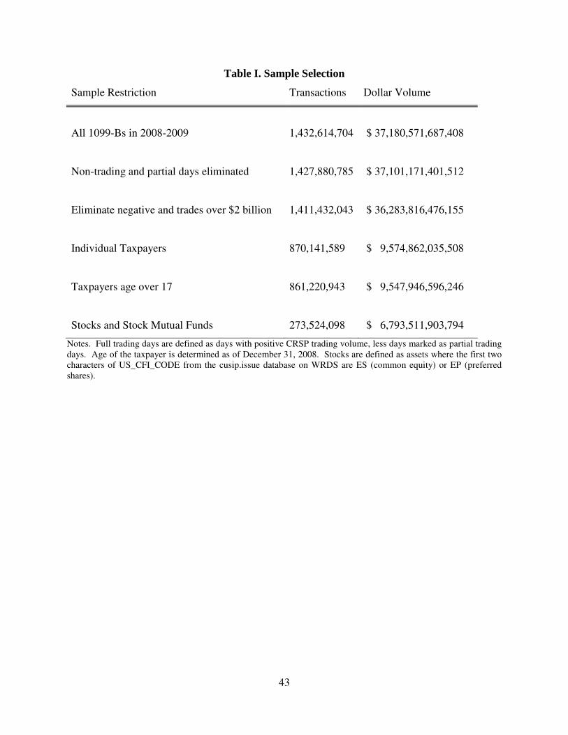
43

Table I. Sample Selection

Sample Restriction Transactions Dollar Volume

All 1099-Bs in 2008-2009

1,432,614,704 $ 37,180,571,687,408

Non-trading and partial days eliminated

1,427,880,785 $ 37,101,171,401,512

Eliminate negative and trades over $2 billion

1,411,432,043 $ 36,283,816,476,155

Individual Taxpayers

870,141,589 $ 9,574,862,035,508

Taxpayers age over 17

861,220,943 $ 9,547,946,596,246

Stocks and Stock Mutual Funds

273,524,098 $ 6,793,511,903,794

Notes. Full trading days are defined as days with positive CRSP trading volume, less days marked as partial trading days. Age of the taxpayer is determined as of December 31, 2008. Stocks are defined as assets where the first two characters of US_CFI_CODE from the cusip.issue database on WRDS are ES (common equity) or EP (preferred shares).

44

Table II. Overall Sales Response to Market Tumult

Dependent variable: log 1099-B sales volume, USD

Sample Period

2008-2009 September - November 2008

Number of 1-day lagged differences: 1 10 1 10

(1) (2) (3) (4)

Change in log VIX 0.346** 4.964*** 0.349*** 7.183***

(0.135) (1.115) (0.131) (1.179)

Observations 498 498 62 62

R-squared 0.01 0.16 0.03 0.54

Notes: 1-day lagged difference is the difference between the lagged and twice lagged value (t-1 and t-2). Columns 2 and 4 report sums of 10 1-day lagged differences (for t-1 and t-2, t-2 and t-3,…, t-10 and t-11). Newey-West standard errors (10-day lag) in parentheses. *** p<0.01, ** p<0.05, * p<0.1

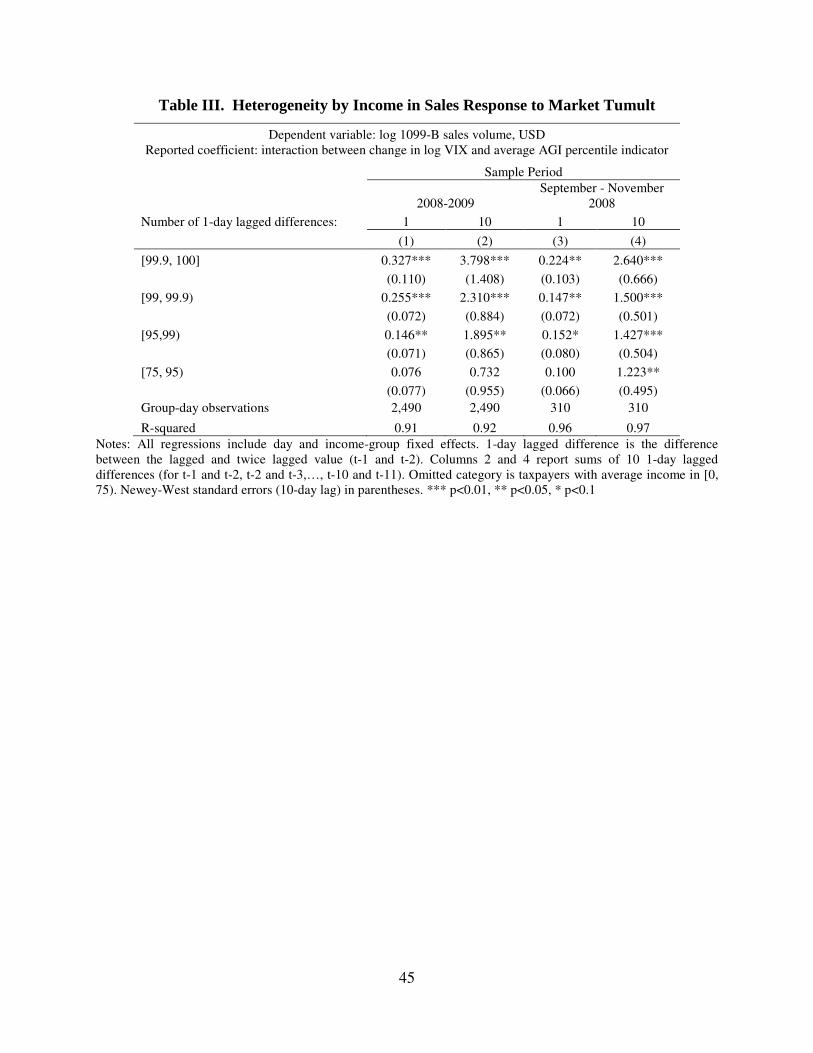
45

Table III. Heterogeneity by Income in Sales Response to Market Tumult

Dependent variable: log 1099-B sales volume, USD Reported coefficient: interaction between change in log VIX and average AGI percentile indicator

Sample Period

2008-2009 September - November

2008

Number of 1-day lagged differences: 1 10 1 10

(1) (2) (3) (4)

[99.9, 100] 0.327*** 3.798*** 0.224** 2.640***

(0.110) (1.408) (0.103) (0.666)

[99, 99.9) 0.255*** 2.310*** 0.147** 1.500***

(0.072) (0.884) (0.072) (0.501)

[95,99) 0.146** 1.895** 0.152* 1.427***

(0.071) (0.865) (0.080) (0.504)

[75, 95) 0.076 0.732 0.100 1.223**

(0.077) (0.955) (0.066) (0.495)

Group-day observations 2,490 2,490 310 310

R-squared 0.91 0.92 0.96 0.97

Notes: All regressions include day and income-group fixed effects. 1-day lagged difference is the difference between the lagged and twice lagged value (t-1 and t-2). Columns 2 and 4 report sums of 10 1-day lagged differences (for t-1 and t-2, t-2 and t-3,…, t-10 and t-11). Omitted category is taxpayers with average income in [0, 75). Newey-West standard errors (10-day lag) in parentheses. *** p<0.01, ** p<0.05, * p<0.1

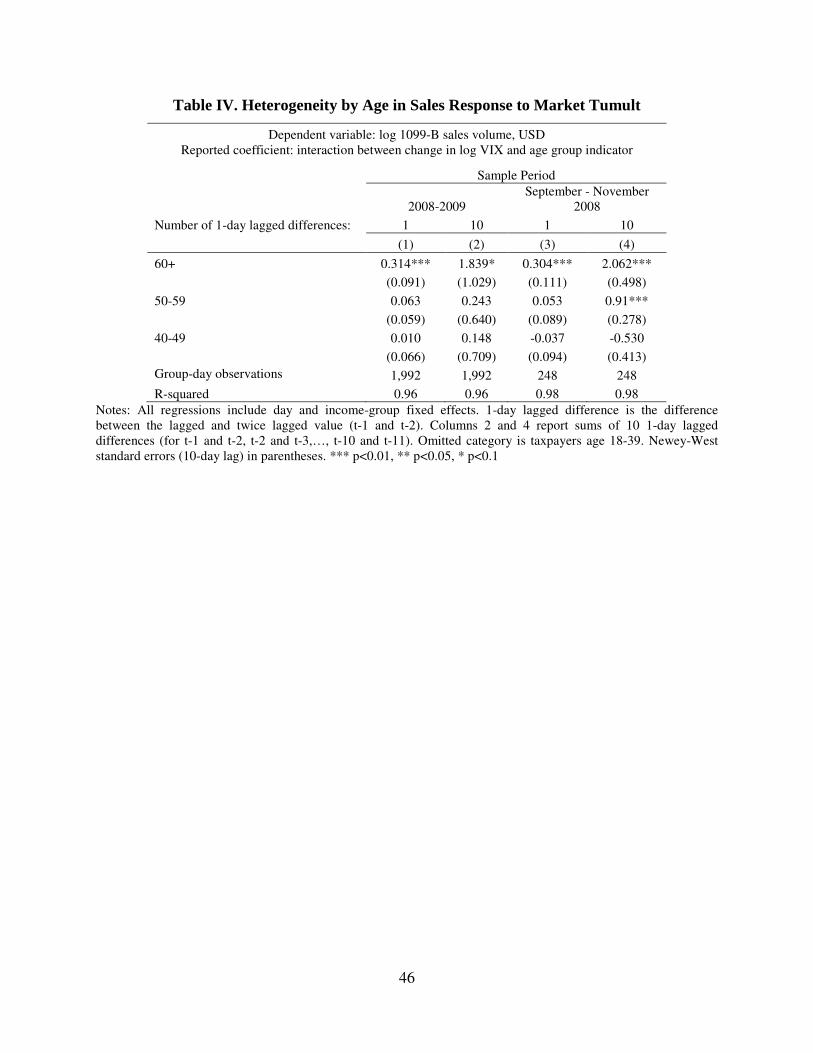
46

Table IV. Heterogeneity by Age in Sales Response to Market Tumult

Dependent variable: log 1099-B sales volume, USD Reported coefficient: interaction between change in log VIX and age group indicator

Sample Period

2008-2009 September - November

2008

Number of 1-day lagged differences: 1 10 1 10

(1) (2) (3) (4)

60+ 0.314*** 1.839* 0.304*** 2.062***

(0.091) (1.029) (0.111) (0.498)

50-59 0.063 0.243 0.053 0.91***

(0.059) (0.640) (0.089) (0.278)

40-49 0.010 0.148 -0.037 -0.530

(0.066) (0.709) (0.094) (0.413)

Group-day observations 1,992 1,992 248 248

R-squared 0.96 0.96 0.98 0.98

Notes: All regressions include day and income-group fixed effects. 1-day lagged difference is the difference between the lagged and twice lagged value (t-1 and t-2). Columns 2 and 4 report sums of 10 1-day lagged differences (for t-1 and t-2, t-2 and t-3,…, t-10 and t-11). Omitted category is taxpayers age 18-39. Newey-West standard errors (10-day lag) in parentheses. *** p<0.01, ** p<0.05, * p<0.1

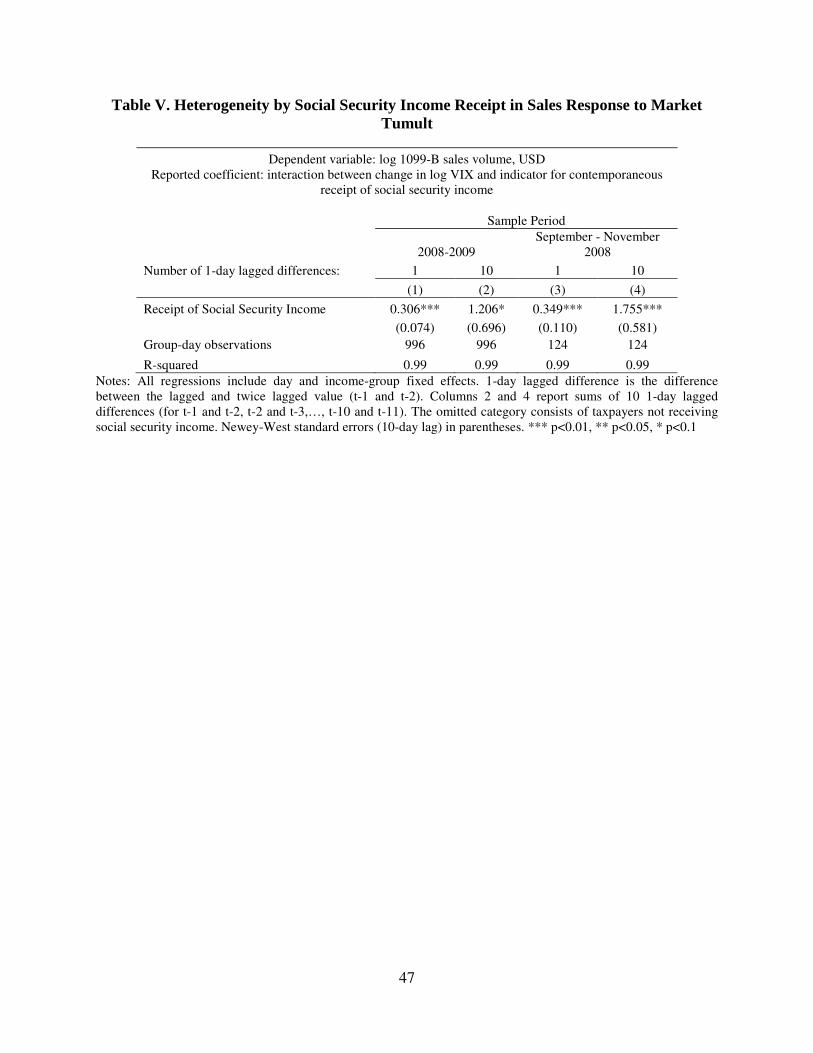
47

Table V. Heterogeneity by Social Security Income Receipt in Sales Response to Market

Tumult

Dependent variable: log 1099-B sales volume, USD Reported coefficient: interaction between change in log VIX and indicator for contemporaneous

receipt of social security income

Sample Period

2008-2009 September - November

2008

Number of 1-day lagged differences: 1 10 1 10

(1) (2) (3) (4)

Receipt of Social Security Income 0.306*** 1.206* 0.349*** 1.755***

(0.074) (0.696) (0.110) (0.581)

Group-day observations 996 996 124 124

R-squared 0.99 0.99 0.99 0.99

Notes: All regressions include day and income-group fixed effects. 1-day lagged difference is the difference between the lagged and twice lagged value (t-1 and t-2). Columns 2 and 4 report sums of 10 1-day lagged differences (for t-1 and t-2, t-2 and t-3,…, t-10 and t-11). The omitted category consists of taxpayers not receiving social security income. Newey-West standard errors (10-day lag) in parentheses. *** p<0.01, ** p<0.05, * p<0.1

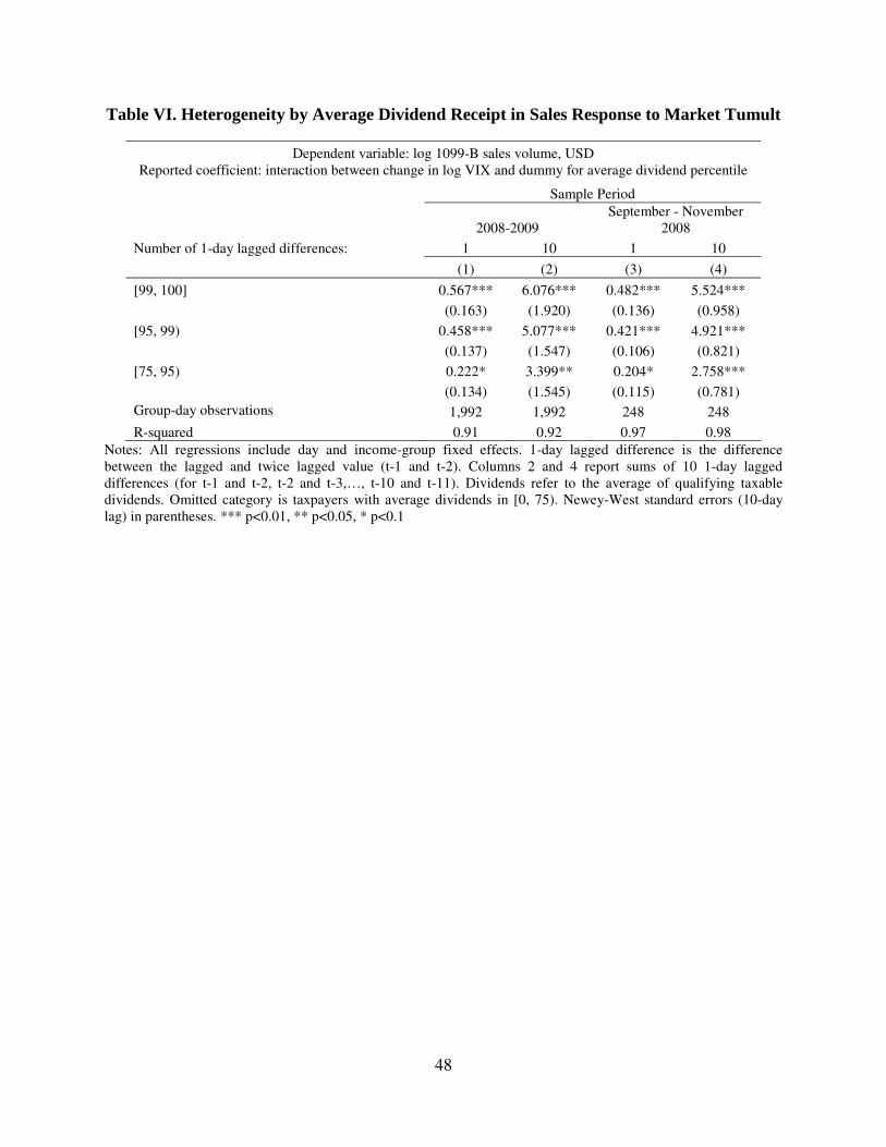
48

Table VI. Heterogeneity by Average Dividend Receipt in Sales Response to Market Tumult

Dependent variable: log 1099-B sales volume, USD Reported coefficient: interaction between change in log VIX and dummy for average dividend percentile

Sample Period

2008-2009 September - November

2008

Number of 1-day lagged differences: 1 10 1 10

(1) (2) (3) (4)

[99, 100] 0.567*** 6.076*** 0.482*** 5.524***

(0.163) (1.920) (0.136) (0.958)

[95, 99) 0.458*** 5.077*** 0.421*** 4.921***

(0.137) (1.547) (0.106) (0.821)

[75, 95) 0.222* 3.399** 0.204* 2.758***

(0.134) (1.545) (0.115) (0.781)

Group-day observations 1,992 1,992 248 248

R-squared 0.91 0.92 0.97 0.98

Notes: All regressions include day and income-group fixed effects. 1-day lagged difference is the difference between the lagged and twice lagged value (t-1 and t-2). Columns 2 and 4 report sums of 10 1-day lagged differences (for t-1 and t-2, t-2 and t-3,…, t-10 and t-11). Dividends refer to the average of qualifying taxable dividends. Omitted category is taxpayers with average dividends in [0, 75). Newey-West standard errors (10-day lag) in parentheses. *** p<0.01, ** p<0.05, * p<0.1

49

Table VII. Heterogeneity by Receipt of Partnership/S-Corp Income in Response to Market

Tumult

Dependent variable: log 1099-B sales volume, USD Reported coefficient: interaction between change in log VIX and dummy for receipt of

positive partnership or S-corporation income

Sample Period

2008-2009 September - November

2008

Number of 1-day lagged differences: 1 10 1 10

(1) (2) (3) (4)

Receipt of Partnership/S-corp Income 0.170*** 1.547*** 0.054 0.444

(0.041) (0.582) (0.044) (0.282)

Group-day observations 996 996 124 124

R-squared 0.97 0.97 0.99 0.99

Notes: All regressions include day and income-group fixed effects. 1-day lagged difference is the difference between the lagged and twice lagged value (t-1 and t-2). Columns 2 and 4 report sums of 10 1-day lagged differences (for t-1 and t-2, t-2 and t-3,…, t-10 and t-11). Omitted category is taxpayers not receiving positive partnership or S-corporation income. Newey-West standard errors (10-day lag) in parentheses. *** p<0.01, ** p<0.05, * p<0.1

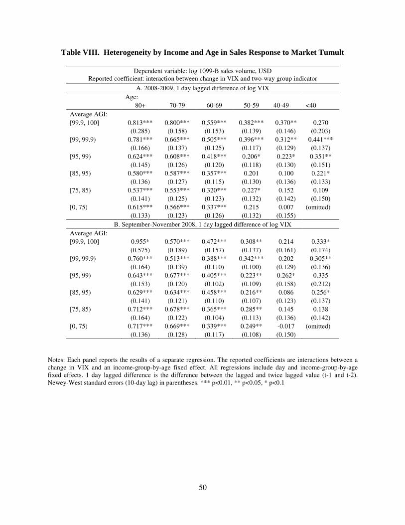
50

Table VIII. Heterogeneity by Income and Age in Sales Response to Market Tumult

Dependent variable: log 1099-B sales volume, USD Reported coefficient: interaction between change in VIX and two-way group indicator

A. 2008-2009, 1 day lagged difference of log VIX

Age:

80+ 70-79 60-69 50-59 40-49 <40

Average AGI:

[99.9, 100] 0.813*** 0.800*** 0.559*** 0.382*** 0.370** 0.270

(0.285) (0.158) (0.153) (0.139) (0.146) (0.203)

[99, 99.9) 0.781*** 0.665*** 0.505*** 0.396*** 0.312** 0.441***

(0.166) (0.137) (0.125) (0.117) (0.129) (0.137)

[95, 99) 0.624*** 0.608*** 0.418*** 0.206* 0.223* 0.351**

(0.145) (0.126) (0.120) (0.118) (0.130) (0.151)

[85, 95) 0.580*** 0.587*** 0.357*** 0.201 0.100 0.221*

(0.136) (0.127) (0.115) (0.130) (0.136) (0.133)

[75, 85) 0.537*** 0.553*** 0.320*** 0.227* 0.152 0.109

(0.141) (0.125) (0.123) (0.132) (0.142) (0.150)

[0, 75) 0.615*** 0.566*** 0.337*** 0.215 0.007 (omitted)

(0.133) (0.123) (0.126) (0.132) (0.155)

B. September-November 2008, 1 day lagged difference of log VIX

Average AGI:

[99.9, 100] 0.955* 0.570*** 0.472*** 0.308** 0.214 0.333*

(0.575) (0.189) (0.157) (0.137) (0.161) (0.174)

[99, 99.9) 0.760*** 0.513*** 0.388*** 0.342*** 0.202 0.305**

(0.164) (0.139) (0.110) (0.100) (0.129) (0.136)

[95, 99) 0.643*** 0.677*** 0.405*** 0.223** 0.262* 0.335

(0.153) (0.120) (0.102) (0.109) (0.158) (0.212)

[85, 95) 0.629*** 0.634*** 0.458*** 0.216** 0.086 0.256*

(0.141) (0.121) (0.110) (0.107) (0.123) (0.137)

[75, 85) 0.712*** 0.678*** 0.365*** 0.285** 0.145 0.138

(0.164) (0.122) (0.104) (0.113) (0.136) (0.142)

[0, 75) 0.717*** 0.669*** 0.339*** 0.249** -0.017 (omitted)

(0.136) (0.128) (0.117) (0.108) (0.150)

Notes: Each panel reports the results of a separate regression. The reported coefficients are interactions between a change in VIX and an income-group-by-age fixed effect. All regressions include day and income-group-by-age fixed effects. 1 day lagged difference is the difference between the lagged and twice lagged value (t-1 and t-2). Newey-West standard errors (10-day lag) in parentheses. *** p<0.01, ** p<0.05, * p<0.1

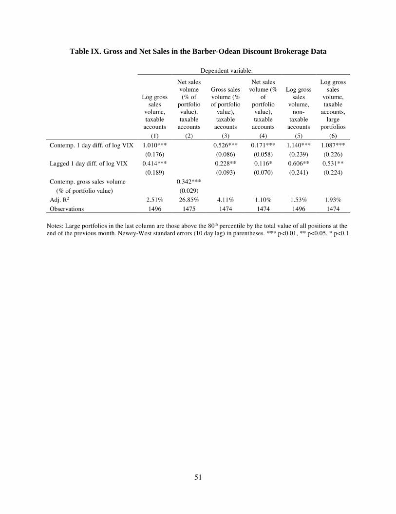
51

Table IX. Gross and Net Sales in the Barber-Odean Discount Brokerage Data

Dependent variable:

Log gross sales

volume, taxable

accounts

Net sales volume (% of

portfolio value), taxable

accounts

Gross sales volume (% of portfolio

value), taxable

accounts

Net sales volume (%

of portfolio value), taxable

accounts

Log gross sales

volume, non-

taxable accounts

Log gross sales

volume, taxable

accounts, large

portfolios

(1) (2) (3) (4) (5) (6)

Contemp. 1 day diff. of log VIX 1.010*** 0.526*** 0.171*** 1.140*** 1.087***

(0.176) (0.086) (0.058) (0.239) (0.226)

Lagged 1 day diff. of log VIX 0.414*** 0.228** 0.116* 0.606** 0.531**

(0.189) (0.093) (0.070) (0.241) (0.224)

Contemp. gross sales volume 0.342***

(% of portfolio value) (0.029)

Adj. R2 2.51% 26.85% 4.11% 1.10% 1.53% 1.93%

Observations 1496 1475 1474 1474 1496 1474

Notes: Large portfolios in the last column are those above the 80th percentile by the total value of all positions at the end of the previous month. Newey-West standard errors (10 day lag) in parentheses. *** p<0.01, ** p<0.05, * p<0.1

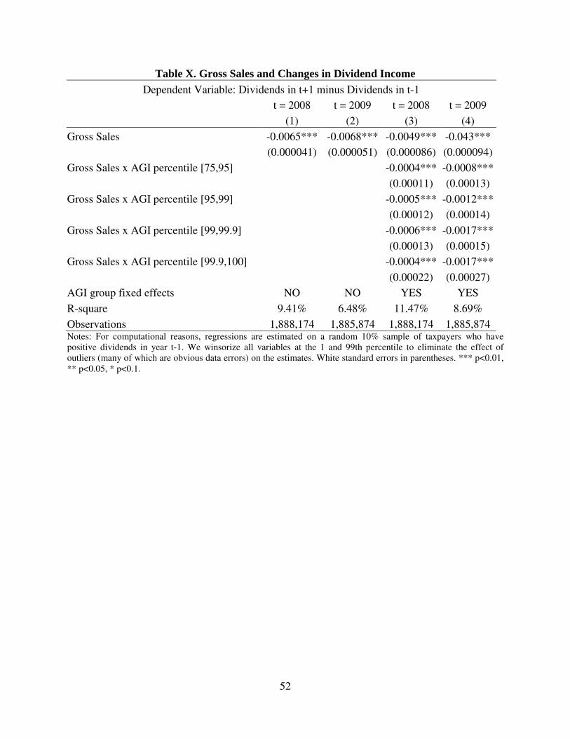
52

Table X. Gross Sales and Changes in Dividend Income

Dependent Variable: Dividends in t+1 minus Dividends in t-1

t = 2008 t = 2009 t = 2008 t = 2009

(1) (2) (3) (4)

Gross Sales -0.0065*** -0.0068*** -0.0049*** -0.043***

(0.000041) (0.000051) (0.000086) (0.000094)

Gross Sales x AGI percentile [75,95] -0.0004*** -0.0008***

(0.00011) (0.00013)

Gross Sales x AGI percentile [95,99] -0.0005*** -0.0012***

(0.00012) (0.00014)

Gross Sales x AGI percentile [99,99.9] -0.0006*** -0.0017***

(0.00013) (0.00015)

Gross Sales x AGI percentile [99.9,100] -0.0004*** -0.0017***

(0.00022) (0.00027)

AGI group fixed effects NO NO YES YES

R-square 9.41% 6.48% 11.47% 8.69%

Observations 1,888,174 1,885,874 1,888,174 1,885,874 Notes: For computational reasons, regressions are estimated on a random 10% sample of taxpayers who have positive dividends in year t-1. We winsorize all variables at the 1 and 99th percentile to eliminate the effect of outliers (many of which are obvious data errors) on the estimates. White standard errors in parentheses. *** p<0.01, ** p<0.05, * p<0.1.

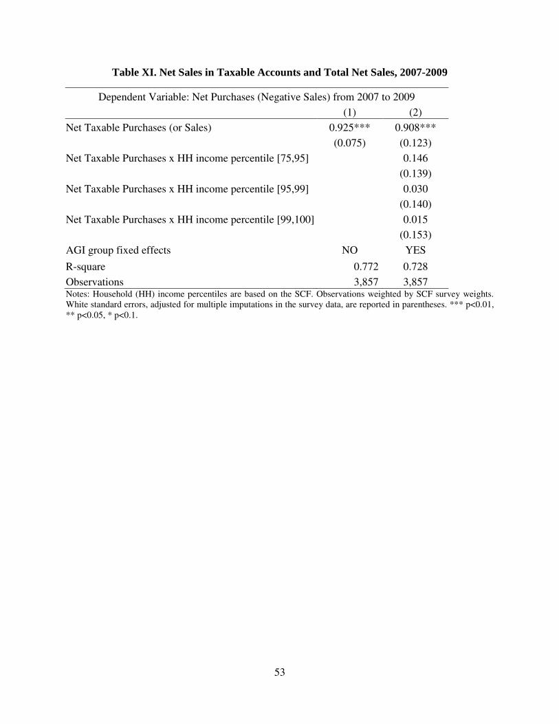
53

Table XI. Net Sales in Taxable Accounts and Total Net Sales, 2007-2009

Dependent Variable: Net Purchases (Negative Sales) from 2007 to 2009

(1) (2)

Net Taxable Purchases (or Sales) 0.925*** 0.908***

(0.075) (0.123)

Net Taxable Purchases x HH income percentile [75,95] 0.146

(0.139)

Net Taxable Purchases x HH income percentile [95,99] 0.030

(0.140)

Net Taxable Purchases x HH income percentile [99,100] 0.015

(0.153)

AGI group fixed effects NO YES

R-square 0.772 0.728

Observations 3,857 3,857 Notes: Household (HH) income percentiles are based on the SCF. Observations weighted by SCF survey weights. White standard errors, adjusted for multiple imputations in the survey data, are reported in parentheses. *** p<0.01, ** p<0.05, * p<0.1.

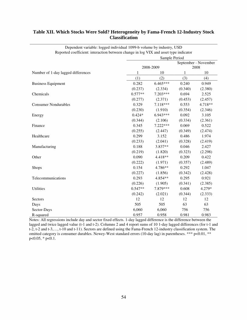
54

Table XII. Which Stocks Were Sold? Heterogeneity by Fama-French 12-Industry Stock

Classification

Dependent variable: logged individual 1099-b volume by industry, USD

Reported coefficient: interaction between change in log VIX and asset type indicator

Sample Period

2008-2009 September - November

2008

Number of 1-day lagged differences 1 10 1 10

(1) (2) (3) (4)

Business Equipment 0.282 6.465*** 0.240 0.949

(0.237) (2.334) (0.340) (2.380)

Chemicals 0.577** 7.203*** 0.694 2.525

(0.277) (2.371) (0.453) (2.457)

Consumer Nondurables 0.329 7.118*** 0.553 4.718**

(0.230) (1.910) (0.354) (2.346)

Energy 0.424* 6.943*** 0.092 3.105

(0.344) (2.106) (0.334) (2.361)

Finance 0.345 7.222*** 0.069 0.522

(0.255) (2.447) (0.349) (2.474)

Healthcare 0.299 3.152 0.486 1.974

(0.233) (2.041) (0.328) (2.419)

Manufacturing 0.188 3.837** 0.046 2.427

(0.219) (1.820) (0.323) (2.298)

Other 0.090 4.418** 0.209 0.422

(0.222) (1.971) (0.357) (2.489)

Shops 0.154 4.786** 0.292 1.047

(0.227) (1.856) (0.342) (2.428)

Telecommunications 0.293 4.854** 0.295 0.921

(0.226) (1.905) (0.341) (2.385)

Utilities 0.547** 7.879*** 0.608 4.279*

(0.242) (2.021) (0.344) (2.333)

Sectors 12 12 12 12

Days 505 505 63 63

Sector-Days 6,060 6,060 756 756

R-squared 0.957 0.958 0.981 0.983

Notes: All regressions include day and sector fixed effects. 1-day lagged difference is the difference between the lagged and twice lagged value (t-1 and t-2). Columns 2 and 4 report sums of 10 1-day lagged differences (for t-1 and t-2, t-2 and t-3,…, t-10 and t-11). Sectors are defined using the Fama-French 12-industry classification system. The omitted category is consumer durables. Newey-West standard errors (10-day lag) in parentheses. *** p<0.01, ** p<0.05, * p<0.1.

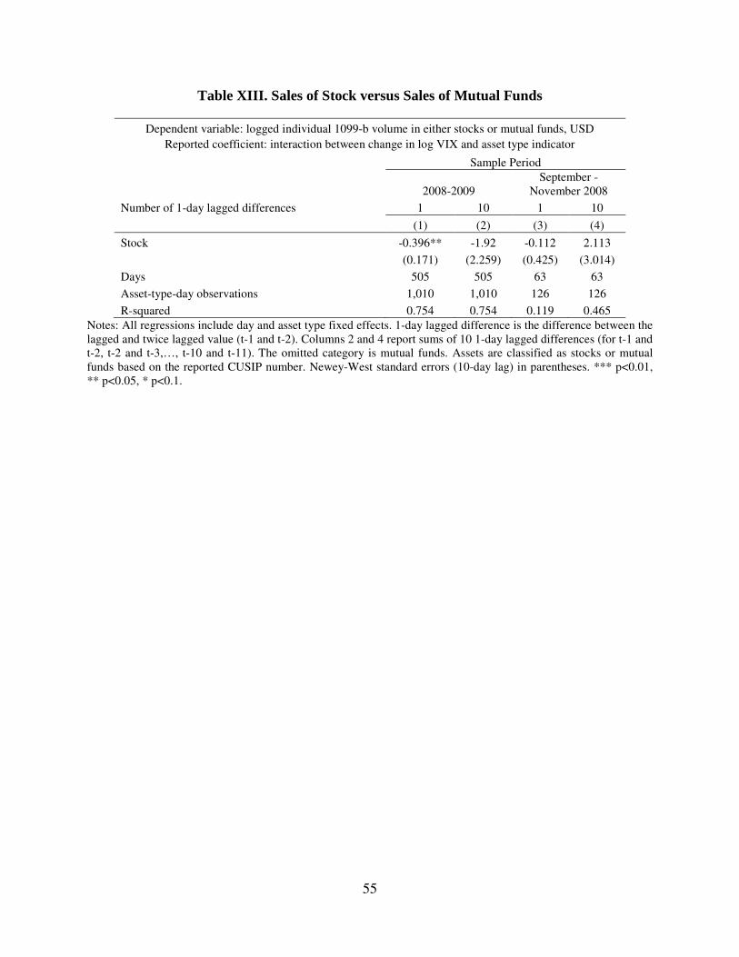
55

Table XIII. Sales of Stock versus Sales of Mutual Funds

Dependent variable: logged individual 1099-b volume in either stocks or mutual funds, USD

Reported coefficient: interaction between change in log VIX and asset type indicator

Sample Period

2008-2009 September -

November 2008

Number of 1-day lagged differences 1 10 1 10

(1) (2) (3) (4)

Stock -0.396** -1.92 -0.112 2.113

(0.171) (2.259) (0.425) (3.014)

Days 505 505 63 63

Asset-type-day observations 1,010 1,010 126 126

R-squared 0.754 0.754 0.119 0.465

Notes: All regressions include day and asset type fixed effects. 1-day lagged difference is the difference between the lagged and twice lagged value (t-1 and t-2). Columns 2 and 4 report sums of 10 1-day lagged differences (for t-1 and t-2, t-2 and t-3,…, t-10 and t-11). The omitted category is mutual funds. Assets are classified as stocks or mutual funds based on the reported CUSIP number. Newey-West standard errors (10-day lag) in parentheses. *** p<0.01, ** p<0.05, * p<0.1.

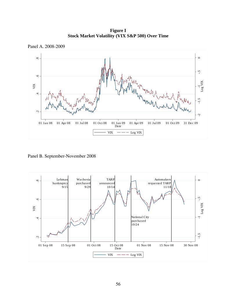
56

Figure I

Stock Market Volatility (VIX S&P 500) Over Time

Panel A. 2008-2009

Panel B. September-November 2008

-2-1

.5-1

-.5

0L

og

VIX

.2.4

.6.8

VIX

01 Jan 08 01 Apr 08 01 Jul 08 01 Oct 08 01 Jan 09 01 Apr 09 01 Jul 09 01 Oct 09 31 Dec 09Date

VIX Log VIX

Lehman

bankruptcy

9/15

Wachovia

purchased

9/29

TARP

announced

10/14

National City

purchased10/24

Automakers

requested TARP

11/18

-1.5

-1-.

50

Log

VIX

.2.4

.6.8

VIX

01 Sep 08 15 Sep 08 01 Oct 08 15 Oct 08 01 Nov 08 15 Nov 08 30 Nov 08Date

VIX Log VIX

57

Figure II

Sales and Trading Volume from Matched 1099-B’s and CRSP

Panel A. Log Sales Volume, Matched 1099-B’s and Universe of Stocks on CRSP

Panel B. Fraction of Total Sales Volume Represented by Matched 1099-B’s

Notes: Total sales volume equals ending price per share times number of shares traded for the universe of stocks on

CRSP. We divide the trading volume of NASDAQ stocks by two because it is a dealer market (see Anderson and

Dyl 2007). The mean and median of the depicted share is 0.059.

91

01

11

21

3L

og

Sa

les V

olu

me, M

illio

ns U

SD

01 Jan 08 01 Apr 08 01 Jul 08 01 Oct 08 01 Jan 09 01 Apr 09 01 Jul 09 01 Oct 09 31 Dec 09Date

CRSP Linked 1099-B

.04

.06

.08

.1.1

2F

ractio

n

01 Jan 08 01 Apr 08 01 Jul 08 01 Oct 08 01 Jan 09 01 Apr 09 01 Jul 09 01 Oct 09 31 Dec 09Date

58

Figure III

Sales Volume and Number of Transactors

Panel A. Sales Volume and Number of Transactors, Matched Form 1099-B’s

Panel B. Average Sales Volume per Transactor, Matched Form 1099-B’s

34

56

78

Num

ber

of T

ran

sacto

rs, 1

00

k

100

00

150

00

200

00

250

00

300

00

Sa

les V

olu

me, M

illio

ns U

SD

01 Jan 08 01 Apr 08 01 Jul 08 01 Oct 08 01 Jan 09 01 Apr 09 01 Jul 09 01 Oct 09 31 Dec 09Date

Linked 1099-B sales volume Transactors

100

00

200

00

300

00

400

00

500

00

Ave

rag

e S

ale

s V

olu

me

per

Tra

nsa

cto

r, U

SD

01 Jan 08 01 Apr 08 01 Jul 08 01 Oct 08 01 Jan 09 01 Apr 09 01 Jul 09 01 Oct 09 31 Dec 09Date

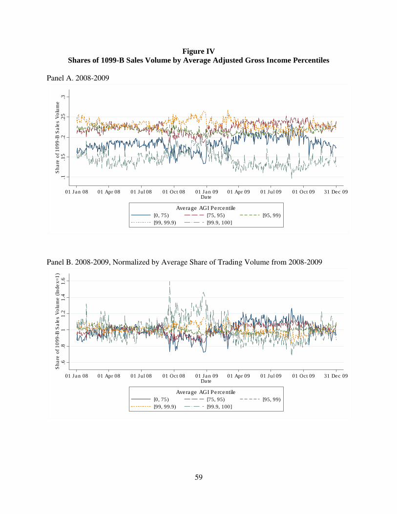
59

Figure IV

Shares of 1099-B Sales Volume by Average Adjusted Gross Income Percentiles

Panel A. 2008-2009

Panel B. 2008-2009, Normalized by Average Share of Trading Volume from 2008-2009

.1.1

5.2

.25

.3S

hare

of 10

99

-B S

ale

s V

olu

me

01 Jan 08 01 Apr 08 01 Jul 08 01 Oct 08 01 Jan 09 01 Apr 09 01 Jul 09 01 Oct 09 31 Dec 09Date

[0, 75) [75, 95) [95, 99)

[99, 99.9) [99.9, 100]

Average AGI Percentile

.6.8

11

.21

.41

.6S

hare

of 10

99

-B S

ale

s V

olu

me (

Inde

x=

1)

01 Jan 08 01 Apr 08 01 Jul 08 01 Oct 08 01 Jan 09 01 Apr 09 01 Jul 09 01 Oct 09 31 Dec 09Date

[0, 75) [75, 95) [95, 99)

[99, 99.9) [99.9, 100]

Average AGI Percentile

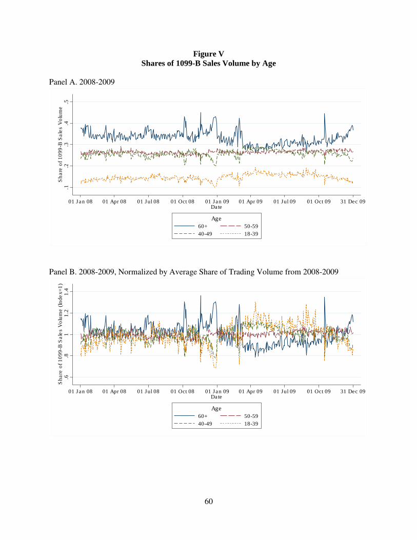
60

Figure V

Shares of 1099-B Sales Volume by Age

Panel A. 2008-2009

Panel B. 2008-2009, Normalized by Average Share of Trading Volume from 2008-2009

.1.2

.3.4

.5S

hare

of 10

99

-B S

ale

s V

olu

me

01 Jan 08 01 Apr 08 01 Jul 08 01 Oct 08 01 Jan 09 01 Apr 09 01 Jul 09 01 Oct 09 31 Dec 09Date

60+ 50-59

40-49 18-39

Age

.6.8

11

.21

.4S

hare

of 10

99

-B S

ale

s V

olu

me (

Inde

x=

1)

01 Jan 08 01 Apr 08 01 Jul 08 01 Oct 08 01 Jan 09 01 Apr 09 01 Jul 09 01 Oct 09 31 Dec 09Date

60+ 50-59

40-49 18-39

Age

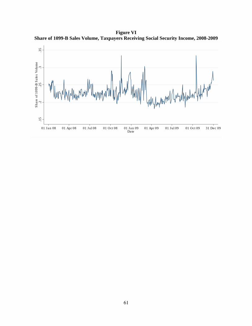
61

Figure VI

Share of 1099-B Sales Volume, Taxpayers Receiving Social Security Income, 2008-2009

.15

.2.2

5.3

.35

Sh

are

of 10

99

-B S

ale

s V

olu

me

01 Jan 08 01 Apr 08 01 Jul 08 01 Oct 08 01 Jan 09 01 Apr 09 01 Jul 09 01 Oct 09 31 Dec 09Date

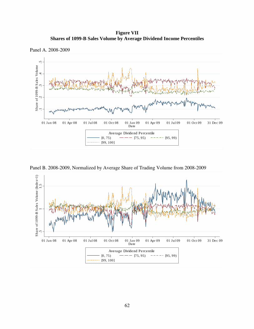
62

Figure VII

Shares of 1099-B Sales Volume by Average Dividend Income Percentiles

Panel A. 2008-2009

Panel B. 2008-2009, Normalized by Average Share of Trading Volume from 2008-2009

.1.2

.3.4

.5S

hare

of 10

99

-B S

ale

s V

olu

me

01 Jan 08 01 Apr 08 01 Jul 08 01 Oct 08 01 Jan 09 01 Apr 09 01 Jul 09 01 Oct 09 31 Dec 09Date

[0, 75) [75, 95) [95, 99)

[99, 100]

Average Dividend Percentile

.51

1.5

Sh

are

of 10

99

-B S

ale

s V

olu

me (

Inde

x=

1)

01 Jan 08 01 Apr 08 01 Jul 08 01 Oct 08 01 Jan 09 01 Apr 09 01 Jul 09 01 Oct 09 31 Dec 09Date

[0, 75) [75, 95) [95, 99)

[99, 100]

Average Dividend Percentile

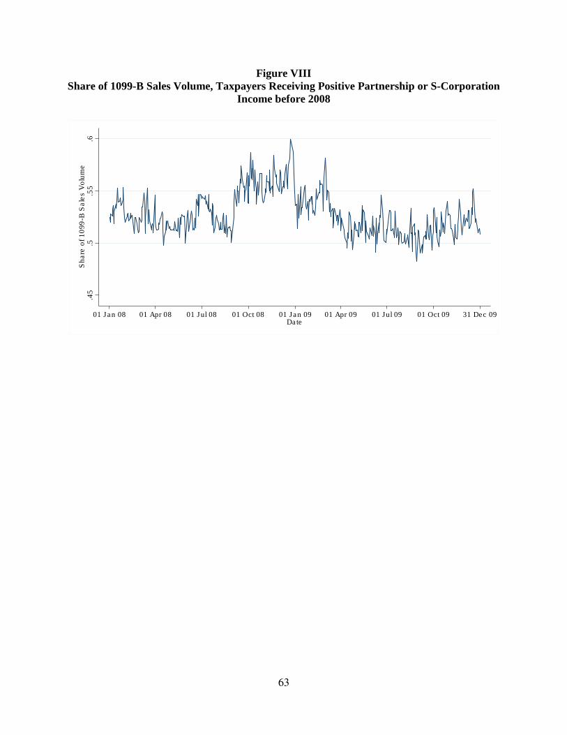
63

Figure VIII

Share of 1099-B Sales Volume, Taxpayers Receiving Positive Partnership or S-Corporation

Income before 2008

.45

.5.5

5.6

Sh

are

of 10

99

-B S

ale

s V

olu

me

01 Jan 08 01 Apr 08 01 Jul 08 01 Oct 08 01 Jan 09 01 Apr 09 01 Jul 09 01 Oct 09 31 Dec 09Date

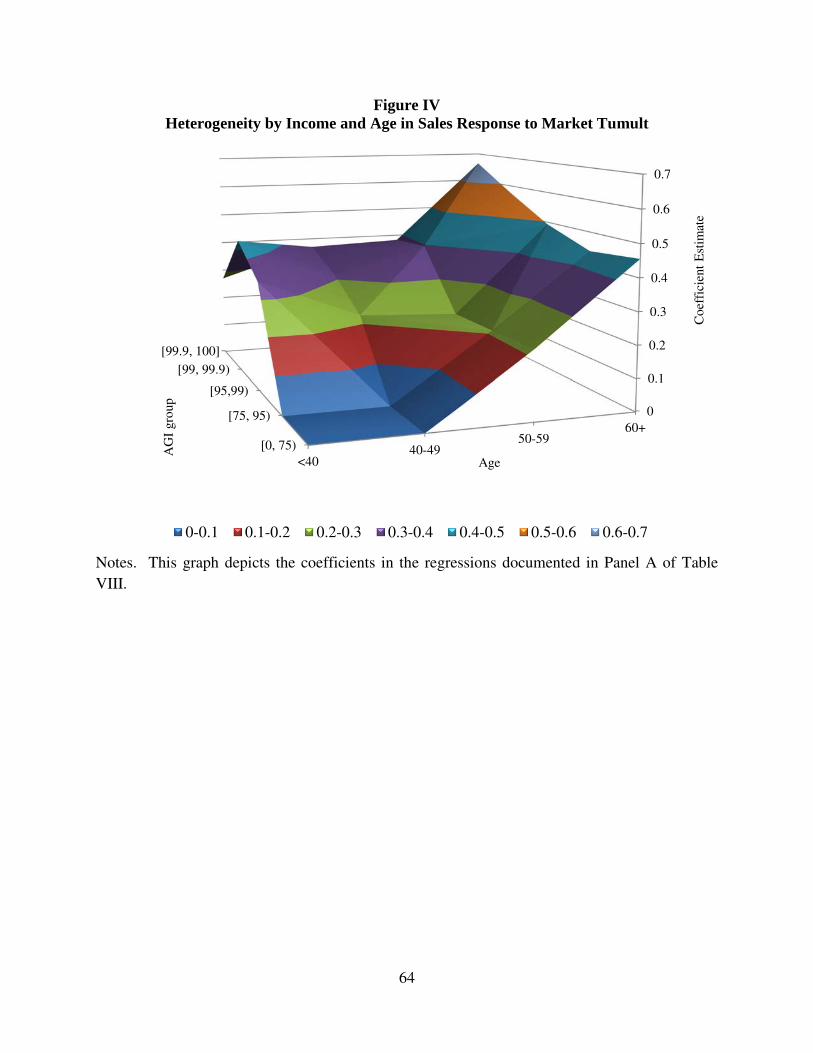
64

Figure IV

Heterogeneity by Income and Age in Sales Response to Market Tumult

Notes. This graph depicts the coefficients in the regressions documented in Panel A of Table

VIII.

[99.9, 100]

[99, 99.9)

[95,99)

[75, 95)

[0, 75)

0

0.1

0.2

0.3

0.4

0.5

0.6

0.7

60+50-59

40-49<40

AG

I gro

up

Co

effi

cien

t E

stim

ate

Age

0-0.1 0.1-0.2 0.2-0.3 0.3-0.4 0.4-0.5 0.5-0.6 0.6-0.7

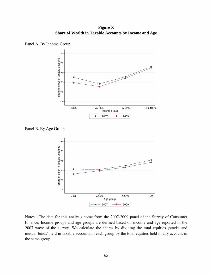
65

Figure X

Share of Wealth in Taxable Accounts by Income and Age

Panel A. By Income Group

Panel B. By Age Group

Notes. The data for this analysis come from the 2007-2009 panel of the Survey of Consumer

Finance. Income groups and age groups are defined based on income and age reported in the

2007 wave of the survey. We calculate the shares by dividing the total equities (stocks and

mutual funds) held in taxable accounts in each group by the total equities held in any account in

the same group.

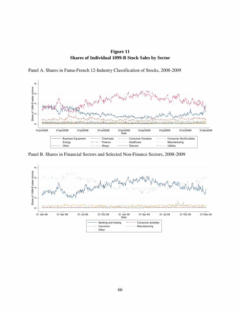
66

Figure 11

Shares of Individual 1099-B Stock Sales by Sector

Panel A. Shares in Fama-French 12-Industry Classification of Stocks, 2008-2009

Panel B. Shares in Financial Sectors and Selected Non-Finance Sectors, 2008-2009

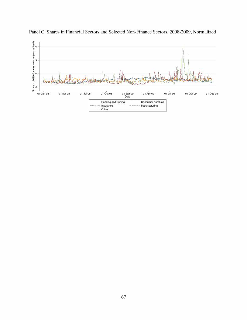
67

Panel C. Shares in Financial Sectors and Selected Non-Finance Sectors, 2008-2009, Normalized

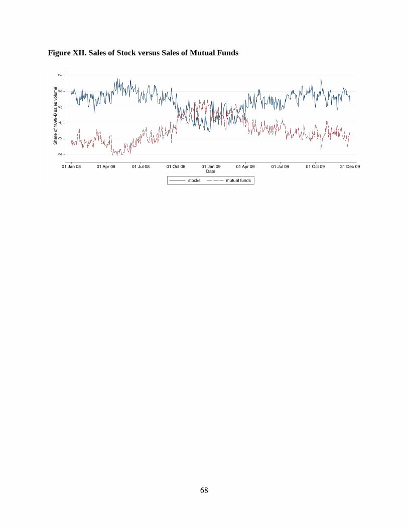
68

Figure XII. Sales of Stock versus Sales of Mutual Funds

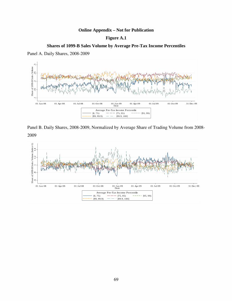
69

Online Appendix – Not for Publication

Figure A.1

Shares of 1099-B Sales Volume by Average Pre-Tax Income Percentiles

Panel A. Daily Shares, 2008-2009

Panel B. Daily Shares, 2008-2009, Normalized by Average Share of Trading Volume from 2008-

2009

.1.1

5.2

.25

.3

Share

of 1099-B

Sale

s V

olu

me

01 Jan 08 01 Apr 08 01 Jul 08 01 Oct 08 01 Jan 09 01 Apr 09 01 Jul 09 01 Oct 09 31 Dec 09Date

[0, 75) [75, 95) [95, 99)

[99, 99.9) [99.9, 100]

Average Pre-Tax Income Percentile

.6.8

11.2

1.4

Share

of 1099-B

Sale

s V

olu

me (In

dex=1)

01 Jan 08 01 Apr 08 01 Jul 08 01 Oct 08 01 Jan 09 01 Apr 09 01 Jul 09 01 Oct 09 31 Dec 09Date

[0, 75) [75, 95) [95, 99)

[99, 99.9) [99.9, 100]

Average Pre-Tax Income Percentile

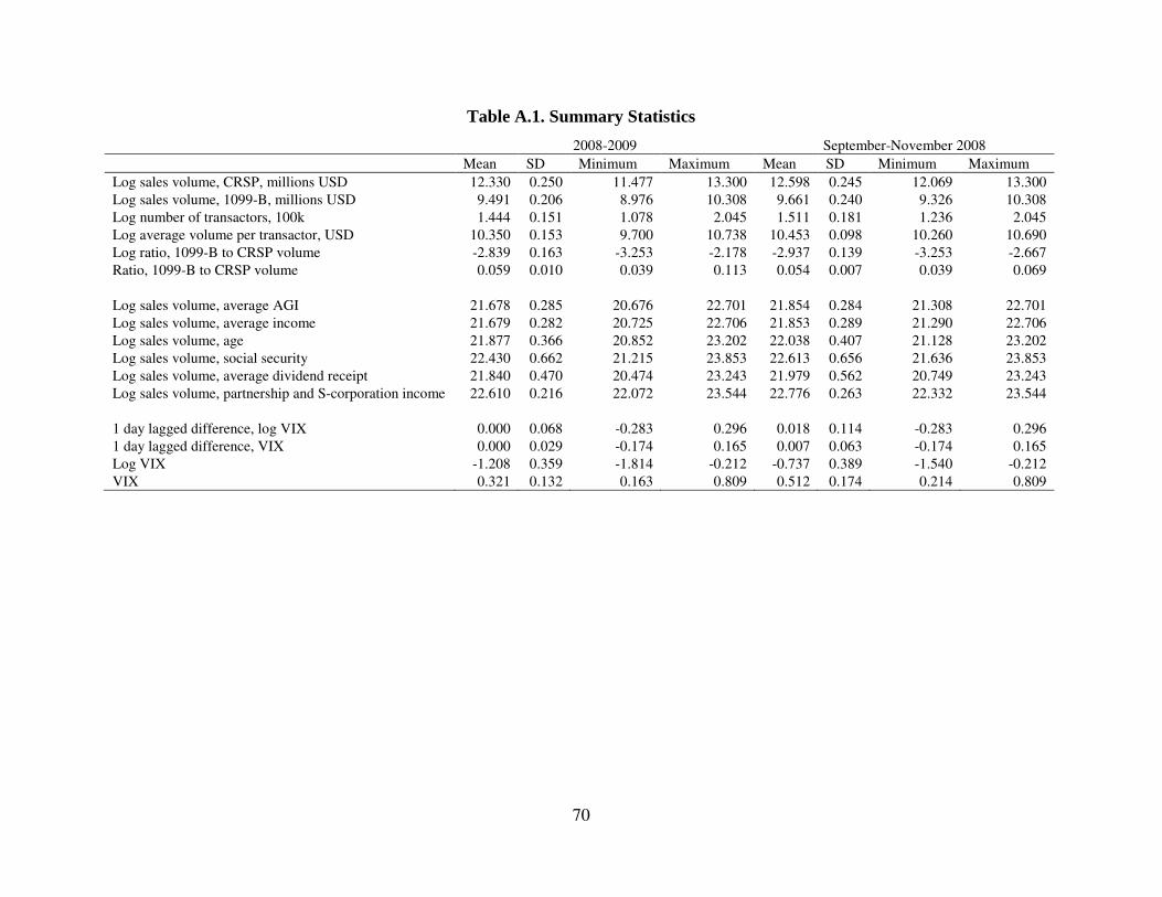
70

Table A.1. Summary Statistics

2008-2009 September-November 2008

Mean SD Minimum Maximum Mean SD Minimum Maximum

Log sales volume, CRSP, millions USD 12.330 0.250 11.477 13.300 12.598 0.245 12.069 13.300

Log sales volume, 1099-B, millions USD 9.491 0.206 8.976 10.308 9.661 0.240 9.326 10.308

Log number of transactors, 100k 1.444 0.151 1.078 2.045 1.511 0.181 1.236 2.045

Log average volume per transactor, USD 10.350 0.153 9.700 10.738 10.453 0.098 10.260 10.690

Log ratio, 1099-B to CRSP volume -2.839 0.163 -3.253 -2.178 -2.937 0.139 -3.253 -2.667

Ratio, 1099-B to CRSP volume 0.059 0.010 0.039 0.113 0.054 0.007 0.039 0.069

Log sales volume, average AGI 21.678 0.285 20.676 22.701 21.854 0.284 21.308 22.701

Log sales volume, average income 21.679 0.282 20.725 22.706 21.853 0.289 21.290 22.706

Log sales volume, age 21.877 0.366 20.852 23.202 22.038 0.407 21.128 23.202

Log sales volume, social security 22.430 0.662 21.215 23.853 22.613 0.656 21.636 23.853

Log sales volume, average dividend receipt 21.840 0.470 20.474 23.243 21.979 0.562 20.749 23.243

Log sales volume, partnership and S-corporation income 22.610 0.216 22.072 23.544 22.776 0.263 22.332 23.544

1 day lagged difference, log VIX 0.000 0.068 -0.283 0.296 0.018 0.114 -0.283 0.296

1 day lagged difference, VIX 0.000 0.029 -0.174 0.165 0.007 0.063 -0.174 0.165

Log VIX -1.208 0.359 -1.814 -0.212 -0.737 0.389 -1.540 -0.212

VIX 0.321 0.132 0.163 0.809 0.512 0.174 0.214 0.809

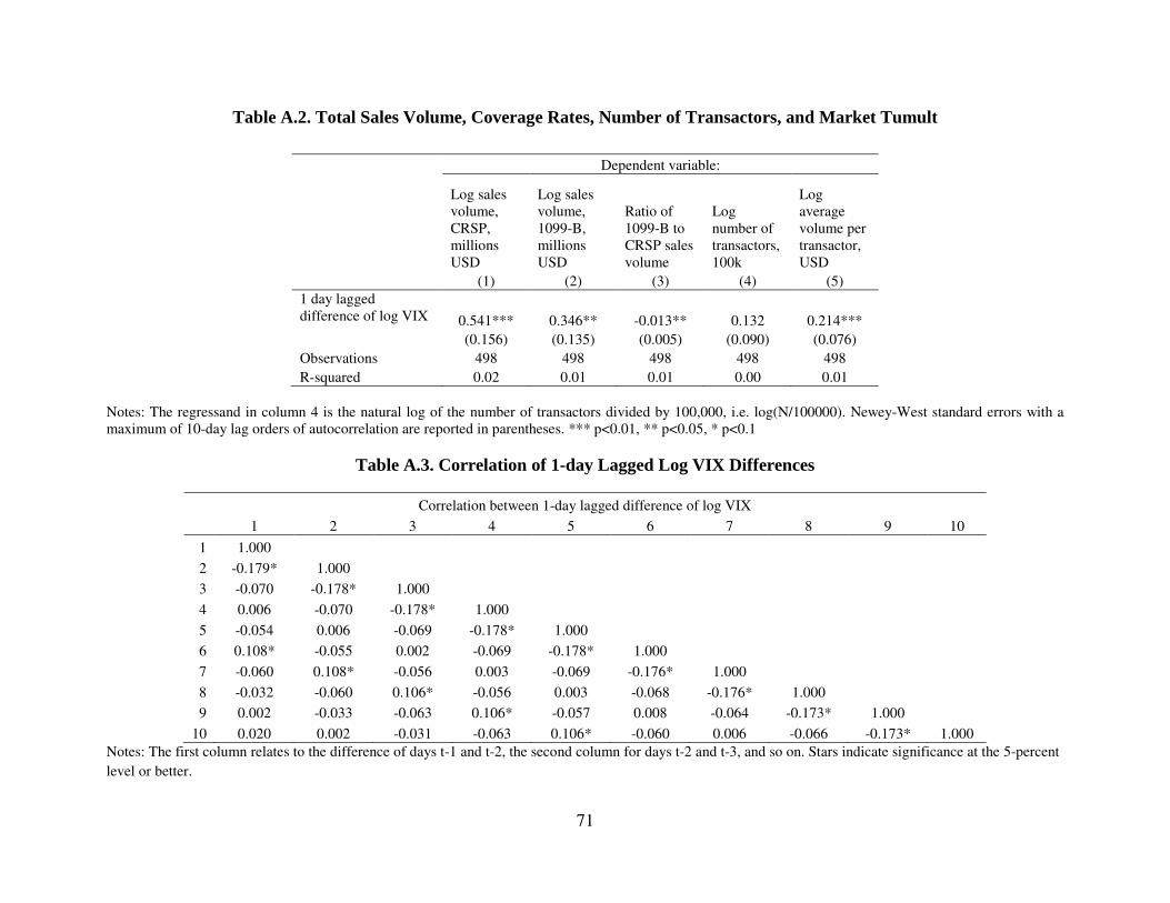
71

Table A.2. Total Sales Volume, Coverage Rates, Number of Transactors, and Market Tumult

Dependent variable:

Log sales volume, CRSP, millions USD

Log sales volume, 1099-B, millions USD

Ratio of 1099-B to CRSP sales volume

Log number of transactors, 100k

Log average volume per transactor, USD

(1) (2) (3) (4) (5)

1 day lagged difference of log VIX 0.541*** 0.346** -0.013** 0.132 0.214***

(0.156) (0.135) (0.005) (0.090) (0.076)

Observations 498 498 498 498 498

R-squared 0.02 0.01 0.01 0.00 0.01

Notes: The regressand in column 4 is the natural log of the number of transactors divided by 100,000, i.e. log(N/100000). Newey-West standard errors with a maximum of 10-day lag orders of autocorrelation are reported in parentheses. *** p<0.01, ** p<0.05, * p<0.1

Table A.3. Correlation of 1-day Lagged Log VIX Differences

Correlation between 1-day lagged difference of log VIX

1 2 3 4 5 6 7 8 9 10

1 1.000

2 -0.179* 1.000

3 -0.070 -0.178* 1.000

4 0.006 -0.070 -0.178* 1.000

5 -0.054 0.006 -0.069 -0.178* 1.000

6 0.108* -0.055 0.002 -0.069 -0.178* 1.000

7 -0.060 0.108* -0.056 0.003 -0.069 -0.176* 1.000

8 -0.032 -0.060 0.106* -0.056 0.003 -0.068 -0.176* 1.000

9 0.002 -0.033 -0.063 0.106* -0.057 0.008 -0.064 -0.173* 1.000

10 0.020 0.002 -0.031 -0.063 0.106* -0.060 0.006 -0.066 -0.173* 1.000

Notes: The first column relates to the difference of days t-1 and t-2, the second column for days t-2 and t-3, and so on. Stars indicate significance at the 5-percent

level or better.

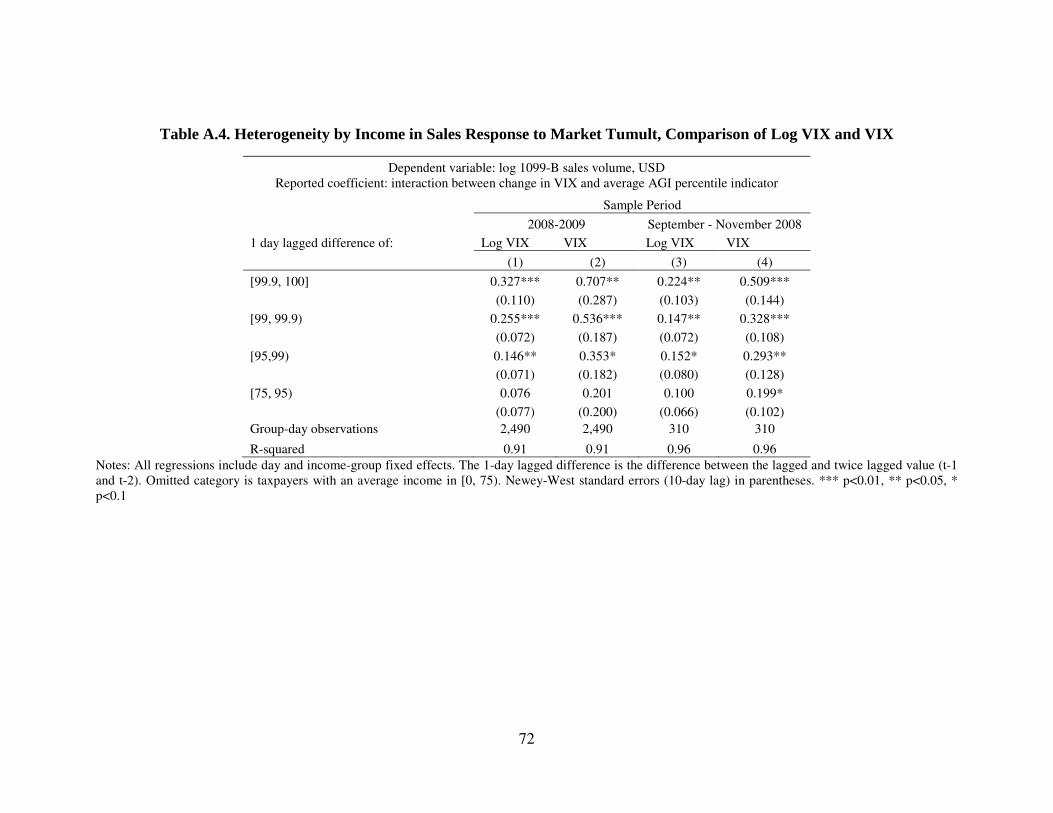
72

Table A.4. Heterogeneity by Income in Sales Response to Market Tumult, Comparison of Log VIX and VIX

Dependent variable: log 1099-B sales volume, USD Reported coefficient: interaction between change in VIX and average AGI percentile indicator

Sample Period

2008-2009 September - November 2008

1 day lagged difference of: Log VIX VIX Log VIX VIX

(1) (2) (3) (4)

[99.9, 100] 0.327*** 0.707** 0.224** 0.509***

(0.110) (0.287) (0.103) (0.144)

[99, 99.9) 0.255*** 0.536*** 0.147** 0.328***

(0.072) (0.187) (0.072) (0.108)

[95,99) 0.146** 0.353* 0.152* 0.293**

(0.071) (0.182) (0.080) (0.128)

[75, 95) 0.076 0.201 0.100 0.199*

(0.077) (0.200) (0.066) (0.102)

Group-day observations 2,490 2,490 310 310

R-squared 0.91 0.91 0.96 0.96

Notes: All regressions include day and income-group fixed effects. The 1-day lagged difference is the difference between the lagged and twice lagged value (t-1 and t-2). Omitted category is taxpayers with an average income in [0, 75). Newey-West standard errors (10-day lag) in parentheses. *** p<0.01, ** p<0.05, * p<0.1

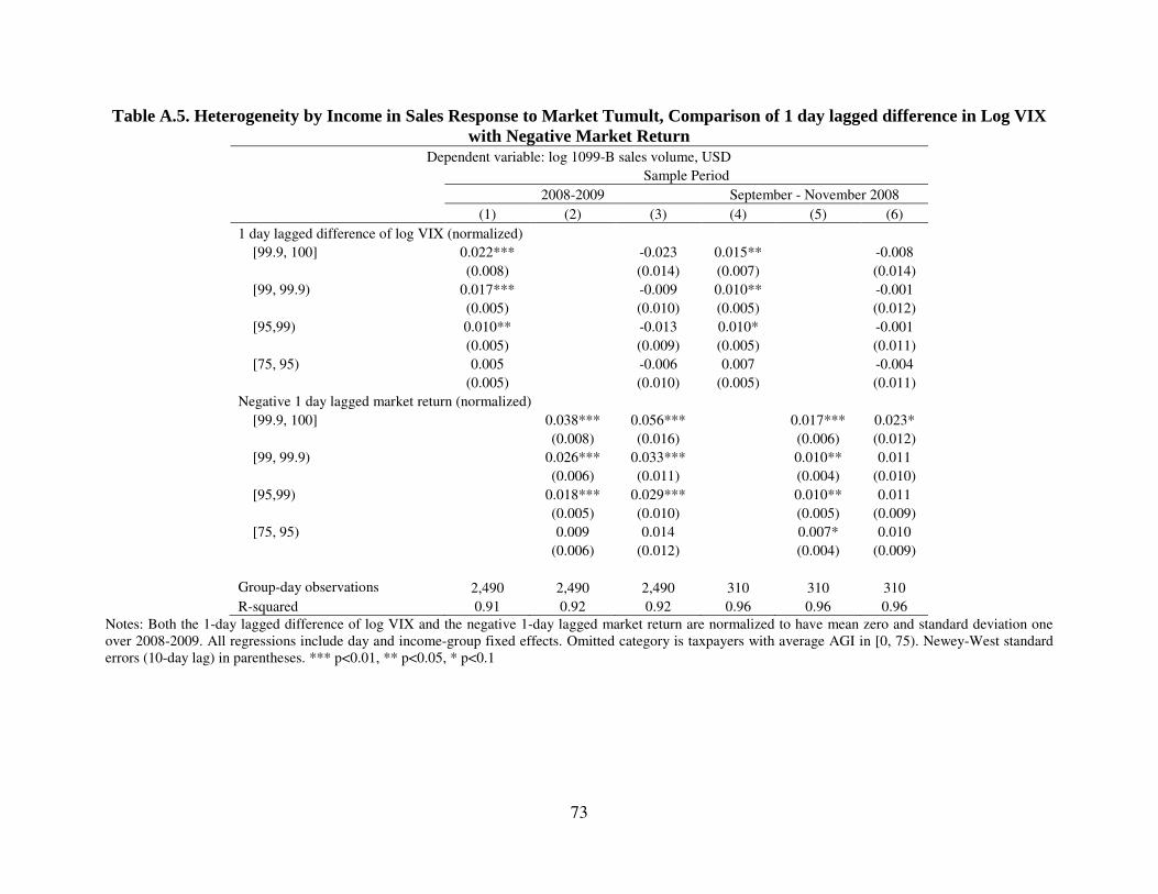
73

Table A.5. Heterogeneity by Income in Sales Response to Market Tumult, Comparison of 1 day lagged difference in Log VIX

with Negative Market Return

Dependent variable: log 1099-B sales volume, USD

Sample Period

2008-2009 September - November 2008

(1) (2) (3) (4) (5) (6)

1 day lagged difference of log VIX (normalized)

[99.9, 100] 0.022*** -0.023 0.015** -0.008

(0.008) (0.014) (0.007) (0.014)

[99, 99.9) 0.017*** -0.009 0.010** -0.001

(0.005) (0.010) (0.005) (0.012)

[95,99) 0.010** -0.013 0.010* -0.001

(0.005) (0.009) (0.005) (0.011)

[75, 95) 0.005 -0.006 0.007 -0.004

(0.005) (0.010) (0.005) (0.011)

Negative 1 day lagged market return (normalized)

[99.9, 100] 0.038*** 0.056*** 0.017*** 0.023*

(0.008) (0.016) (0.006) (0.012)

[99, 99.9) 0.026*** 0.033*** 0.010** 0.011

(0.006) (0.011) (0.004) (0.010)

[95,99) 0.018*** 0.029*** 0.010** 0.011

(0.005) (0.010) (0.005) (0.009)

[75, 95) 0.009 0.014 0.007* 0.010

(0.006) (0.012) (0.004) (0.009)

Group-day observations 2,490 2,490 2,490 310 310 310

R-squared 0.91 0.92 0.92 0.96 0.96 0.96

Notes: Both the 1-day lagged difference of log VIX and the negative 1-day lagged market return are normalized to have mean zero and standard deviation one over 2008-2009. All regressions include day and income-group fixed effects. Omitted category is taxpayers with average AGI in [0, 75). Newey-West standard errors (10-day lag) in parentheses. *** p<0.01, ** p<0.05, * p<0.1

74

Table A.6. Lag Structure of Heterogeneity by Income in Sales Response to Market Tumult, 2008-2009

Dependent variable: log 1099-B sales volume, USD Reported coefficient: interaction between lagged difference of log VIX and

average AGI percentile indicator

[75, 95) [95,99) [99, 99.9) [99.9, 100]

Leads (t+5) - (t+4) 0.002 0.036 0.009 0.114

(0.091) (0.080) (0.084) (0.131)

(t+4) - (t+3) 0.024 0.027 -0.013 0.109

(0.102) (0.090) (0.093) (0.151)

(t+3) - (t+2) 0.002 0.006 -0.050 -0.046

(0.109) (0.096) (0.101) (0.157)

(t+2) - (t+1) -0.002 0.042 0.007 0.029

(0.115) (0.104) (0.110) (0.168)

(t+1) - (t) -0.001 0.017 -0.002 -0.047

(0.120) (0.109) (0.114) (0.173)

Lags (t) - (t-1) 0.061 0.249** 0.395*** 0.422**

(0.115) (0.106) (0.111) (0.164)

(t-1) - (t-2) 0.098 0.222** 0.370*** 0.448***

(0.118) (0.107) (0.111) (0.166)

(t-2) - (t-3) 0.113 0.220* 0.289** 0.396**

(0.129) (0.114) (0.118) (0.190)

(t-3) - (t-4) 0.057 0.192* 0.223* 0.329*

(0.130) (0.117) (0.122) (0.188)

(t-4) - (t-5) 0.079 0.207* 0.257** 0.419**

(0.136) (0.122) (0.125) (0.205)

(t-5) - (t-6) 0.060 0.169 0.255** 0.390**

(0.124) (0.112) (0.117) (0.178)

(t-6) - (t-7) 0.072 0.150 0.174* 0.319*

(0.111) (0.103) (0.104) (0.169)

(t-7) - (t-8) 0.030 0.138 0.153 0.304**

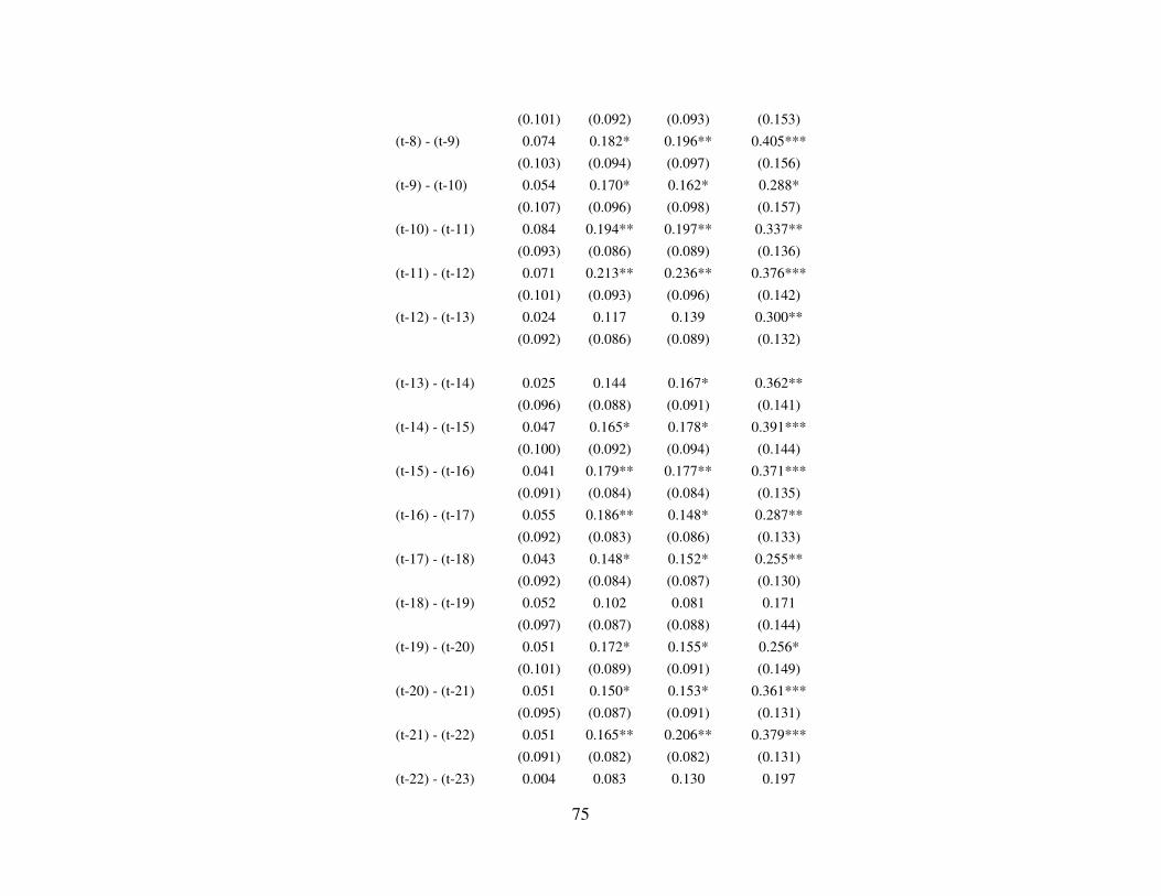
75

(0.101) (0.092) (0.093) (0.153)

(t-8) - (t-9) 0.074 0.182* 0.196** 0.405***

(0.103) (0.094) (0.097) (0.156)

(t-9) - (t-10) 0.054 0.170* 0.162* 0.288*

(0.107) (0.096) (0.098) (0.157)

(t-10) - (t-11) 0.084 0.194** 0.197** 0.337**

(0.093) (0.086) (0.089) (0.136)

(t-11) - (t-12) 0.071 0.213** 0.236** 0.376***

(0.101) (0.093) (0.096) (0.142)

(t-12) - (t-13) 0.024 0.117 0.139 0.300**

(0.092) (0.086) (0.089) (0.132)

(t-13) - (t-14) 0.025 0.144 0.167* 0.362**

(0.096) (0.088) (0.091) (0.141)

(t-14) - (t-15) 0.047 0.165* 0.178* 0.391***

(0.100) (0.092) (0.094) (0.144)

(t-15) - (t-16) 0.041 0.179** 0.177** 0.371***

(0.091) (0.084) (0.084) (0.135)

(t-16) - (t-17) 0.055 0.186** 0.148* 0.287**

(0.092) (0.083) (0.086) (0.133)

(t-17) - (t-18) 0.043 0.148* 0.152* 0.255**

(0.092) (0.084) (0.087) (0.130)

(t-18) - (t-19) 0.052 0.102 0.081 0.171

(0.097) (0.087) (0.088) (0.144)

(t-19) - (t-20) 0.051 0.172* 0.155* 0.256*

(0.101) (0.089) (0.091) (0.149)

(t-20) - (t-21) 0.051 0.150* 0.153* 0.361***

(0.095) (0.087) (0.091) (0.131)

(t-21) - (t-22) 0.051 0.165** 0.206** 0.379***

(0.091) (0.082) (0.082) (0.131)

(t-22) - (t-23) 0.004 0.083 0.130 0.197

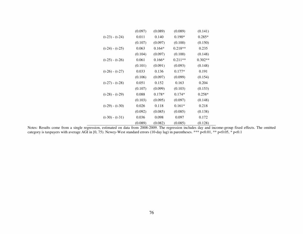
76

(0.097) (0.089) (0.089) (0.141)

(t-23) - (t-24) 0.011 0.140 0.190* 0.285*

(0.107) (0.097) (0.100) (0.150)

(t-24) - (t-25) 0.063 0.164* 0.218** 0.235

(0.104) (0.097) (0.100) (0.148)

(t-25) - (t-26) 0.061 0.166* 0.211** 0.302**

(0.101) (0.091) (0.093) (0.148)

(t-26) - (t-27) 0.033 0.136 0.177* 0.191

(0.106) (0.097) (0.099) (0.154)

(t-27) - (t-28) 0.051 0.152 0.163 0.204

(0.107) (0.099) (0.103) (0.153)

(t-28) - (t-29) 0.088 0.178* 0.174* 0.258*

(0.103) (0.095) (0.097) (0.148)

(t-29) - (t-30) 0.026 0.118 0.161* 0.218

(0.092) (0.085) (0.085) (0.138)

(t-30) - (t-31) 0.036 0.098 0.097 0.172

(0.089) (0.082) (0.085) (0.128)

Notes: Results come from a single regression, estimated on data from 2008-2009. The regression includes day and income-group fixed effects. The omitted category is taxpayers with average AGI in [0, 75). Newey-West standard errors (10-day lag) in parentheses. *** p<0.01, ** p<0.05, * p<0.1

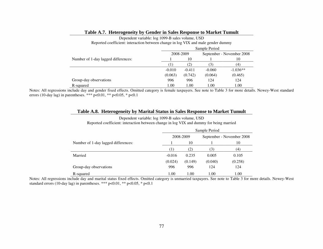
77

Table A.7. Heterogeneity by Gender in Sales Response to Market Tumult

Dependent variable: log 1099-B sales volume, USD Reported coefficient: interaction between change in log VIX and male gender dummy

Sample Period

2008-2009 September - November 2008

Number of 1-day lagged differences: 1 10 1 10

(1) (2) (3) (4)

-0.010 -0.411 -0.060 -1.036**

(0.063) (0.742) (0.064) (0.465)

Group-day observations 996 996 124 124

R-squared 1.00 1.00 1.00 1.00

Notes: All regressions include day and gender fixed effects. Omitted category is female taxpayers. See note to Table 3 for more details. Newey-West standard errors (10-day lag) in parentheses. *** p<0.01, ** p<0.05, * p<0.1

Table A.8. Heterogeneity by Marital Status in Sales Response to Market Tumult

Dependent variable: log 1099-B sales volume, USD Reported coefficient: interaction between change in log VIX and dummy for being married

Sample Period

2008-2009 September - November 2008

Number of 1-day lagged differences: 1 10 1 10

(1) (2) (3) (4)

Married -0.016 0.235 0.005 0.105

(0.024) (0.149) (0.040) (0.258)

Group-day observations 996 996 124 124

R-squared 1.00 1.00 1.00 1.00

Notes: All regressions include day and marital status fixed effects. Omitted category is unmarried taxpayers. See note to Table 3 for more details. Newey-West standard errors (10-day lag) in parentheses. *** p<0.01, ** p<0.05, * p<0.1

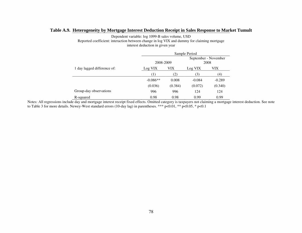
78

Table A.9. Heterogeneity by Mortgage Interest Deduction Receipt in Sales Response to Market Tumult

Dependent variable: log 1099-B sales volume, USD Reported coefficient: interaction between change in log VIX and dummy for claiming mortgage

interest deduction in given year

Sample Period

2008-2009 September - November

2008

1 day lagged difference of: Log VIX VIX Log VIX VIX

(1) (2) (3) (4)

-0.086** 0.008 -0.084 -0.289

(0.036) (0.384) (0.072) (0.340)

Group-day observations 996 996 124 124

R-squared 0.98 0.98 0.99 0.99

Notes: All regressions include day and mortgage interest receipt fixed effects. Omitted category is taxpayers not claiming a mortgage interest deduction. See note to Table 3 for more details. Newey-West standard errors (10-day lag) in parentheses. *** p<0.01, ** p<0.05, * p<0.1

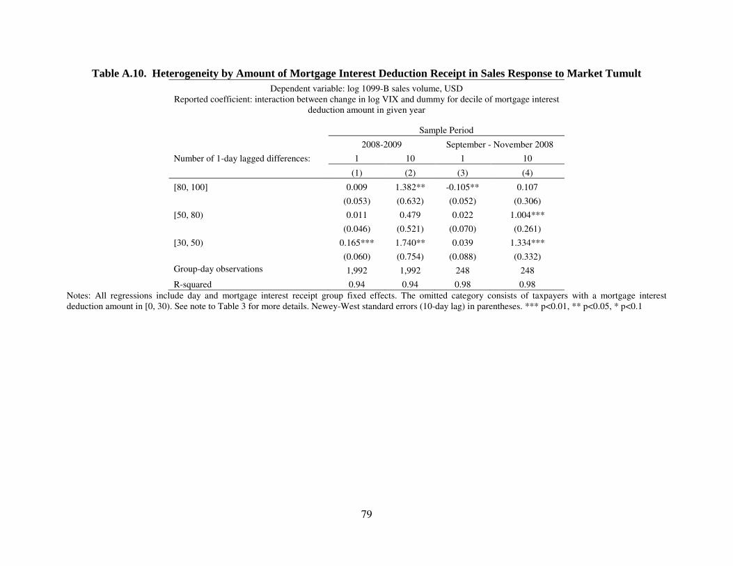
79

Table A.10. Heterogeneity by Amount of Mortgage Interest Deduction Receipt in Sales Response to Market Tumult

Dependent variable: log 1099-B sales volume, USD Reported coefficient: interaction between change in log VIX and dummy for decile of mortgage interest

deduction amount in given year

Sample Period

2008-2009 September - November 2008

Number of 1-day lagged differences: 1 10 1 10

(1) (2) (3) (4)

[80, 100] 0.009 1.382** -0.105** 0.107

(0.053) (0.632) (0.052) (0.306)

[50, 80) 0.011 0.479 0.022 1.004***

(0.046) (0.521) (0.070) (0.261)

[30, 50) 0.165*** 1.740** 0.039 1.334***

(0.060) (0.754) (0.088) (0.332)

Group-day observations 1,992 1,992 248 248

R-squared 0.94 0.94 0.98 0.98

Notes: All regressions include day and mortgage interest receipt group fixed effects. The omitted category consists of taxpayers with a mortgage interest deduction amount in [0, 30). See note to Table 3 for more details. Newey-West standard errors (10-day lag) in parentheses. *** p<0.01, ** p<0.05, * p<0.1

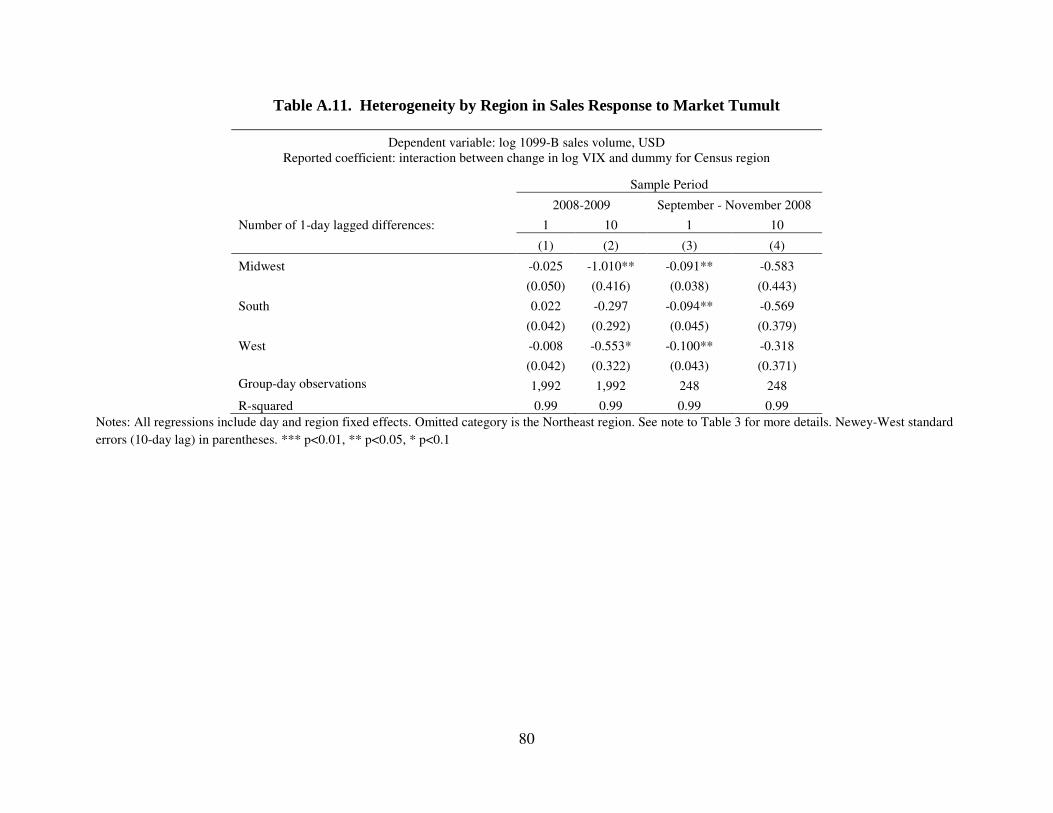
80

Table A.11. Heterogeneity by Region in Sales Response to Market Tumult

Dependent variable: log 1099-B sales volume, USD Reported coefficient: interaction between change in log VIX and dummy for Census region

Sample Period

2008-2009 September - November 2008

Number of 1-day lagged differences: 1 10 1 10

(1) (2) (3) (4)

Midwest -0.025 -1.010** -0.091** -0.583

(0.050) (0.416) (0.038) (0.443)

South 0.022 -0.297 -0.094** -0.569

(0.042) (0.292) (0.045) (0.379)

West -0.008 -0.553* -0.100** -0.318

(0.042) (0.322) (0.043) (0.371)

Group-day observations 1,992 1,992 248 248

R-squared 0.99 0.99 0.99 0.99

Notes: All regressions include day and region fixed effects. Omitted category is the Northeast region. See note to Table 3 for more details. Newey-West standard

errors (10-day lag) in parentheses. *** p<0.01, ** p<0.05, * p<0.1

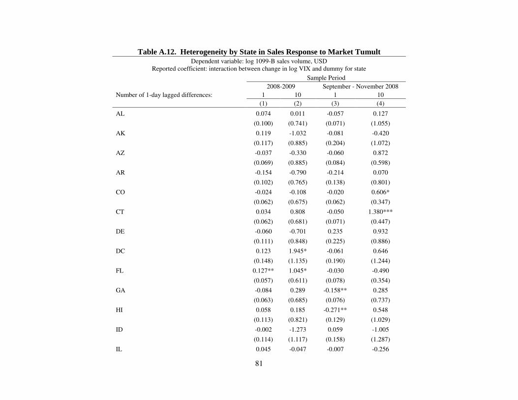
81

Table A.12. Heterogeneity by State in Sales Response to Market Tumult Dependent variable: log 1099-B sales volume, USD

Reported coefficient: interaction between change in log VIX and dummy for state

Sample Period

2008-2009 September - November 2008

Number of 1-day lagged differences: 1 10 1 10

(1) (2) (3) (4)

AL 0.074 0.011 -0.057 0.127

(0.100) (0.741) (0.071) (1.055)

AK 0.119 -1.032 -0.081 -0.420

(0.117) (0.885) (0.204) (1.072)

AZ -0.037 -0.330 -0.060 0.872

(0.069) (0.885) (0.084) (0.598)

AR -0.154 -0.790 -0.214 0.070

(0.102) (0.765) (0.138) (0.801)

CO -0.024 -0.108 -0.020 0.606*

(0.062) (0.675) (0.062) (0.347)

CT 0.034 0.808 -0.050 1.380***

(0.062) (0.681) (0.071) (0.447)

DE -0.060 -0.701 0.235 0.932

(0.111) (0.848) (0.225) (0.886)

DC 0.123 1.945* -0.061 0.646

(0.148) (1.135) (0.190) (1.244)

FL 0.127** 1.045* -0.030 -0.490

(0.057) (0.611) (0.078) (0.354)

GA -0.084 0.289 -0.158** 0.285

(0.063) (0.685) (0.076) (0.737)

HI 0.058 0.185 -0.271** 0.548

(0.113) (0.821) (0.129) (1.029)

ID -0.002 -1.273 0.059 -1.005

(0.114) (1.117) (0.158) (1.287)

IL 0.045 -0.047 -0.007 -0.256

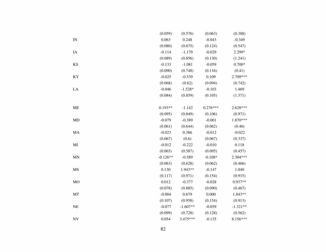
82

(0.059) (0.576) (0.063) (0.388)

IN 0.063 0.248 -0.043 -0.349

(0.080) (0.675) (0.124) (0.547)

IA -0.114 -1.179 -0.029 2.299*

(0.089) (0.856) (0.130) (1.241)

KS -0.133 -1.081 -0.059 0.700*

(0.090) (0.748) (0.116) (0.41)

KY -0.025 -0.539 0.109 2.709***

(0.068) (0.62) (0.094) (0.742)

LA -0.046 -1.528* -0.103 1.469

(0.084) (0.859) (0.105) (1.371)

ME 0.193** -1.142 0.276*** 2.628***

(0.095) (0.849) (0.106) (0.971)

MD -0.079 -0.389 -0.001 1.870***

(0.061) (0.644) (0.062) (0.46)

MA -0.023 0.386 -0.012 -0.022

(0.067) (0.6) (0.067) (0.337)

MI -0.012 -0.222 -0.010 0.118

(0.065) (0.587) (0.095) (0.457)

MN -0.126** -0.589 -0.108* 2.304***

(0.063) (0.628) (0.062) (0.466)

MS 0.130 1.943** -0.147 1.040

(0.117) (0.971) (0.154) (0.915)

MO 0.012 -0.377 -0.028 0.937**

(0.078) (0.885) (0.090) (0.467)

MT -0.004 0.679 0.000 1.843**

(0.107) (0.958) (0.154) (0.913)

NE -0.077 -1.607** -0.059 -1.321**

(0.099) (0.728) (0.128) (0.562)

NV 0.054 3.475*** -0.135 8.156***

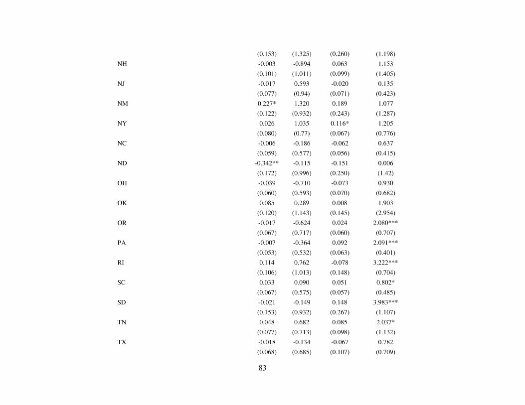
83

(0.153) (1.325) (0.260) (1.198)

NH -0.003 -0.894 0.063 1.153

(0.101) (1.011) (0.099) (1.405)

NJ -0.017 0.593 -0.020 0.135

(0.077) (0.94) (0.071) (0.423)

NM 0.227* 1.320 0.189 1.077

(0.122) (0.932) (0.243) (1.287)

NY 0.026 1.035 0.116* 1.205

(0.080) (0.77) (0.067) (0.776)

NC -0.006 -0.186 -0.062 0.637

(0.059) (0.577) (0.056) (0.415)

ND -0.342** -0.115 -0.151 0.006

(0.172) (0.996) (0.250) (1.42)

OH -0.039 -0.710 -0.073 0.930

(0.060) (0.593) (0.070) (0.682)

OK 0.085 0.289 0.008 1.903

(0.120) (1.143) (0.145) (2.954)

OR -0.017 -0.624 0.024 2.080***

(0.067) (0.717) (0.060) (0.707)

PA -0.007 -0.364 0.092 2.091***

(0.053) (0.532) (0.063) (0.401)

RI 0.114 0.762 -0.078 3.222***

(0.106) (1.013) (0.148) (0.704)

SC 0.033 0.090 0.051 0.802*

(0.067) (0.575) (0.057) (0.485)

SD -0.021 -0.149 0.148 3.983***

(0.153) (0.932) (0.267) (1.107)

TN 0.048 0.682 0.085 2.037*

(0.077) (0.713) (0.098) (1.132)

TX -0.018 -0.134 -0.067 0.782

(0.068) (0.685) (0.107) (0.709)

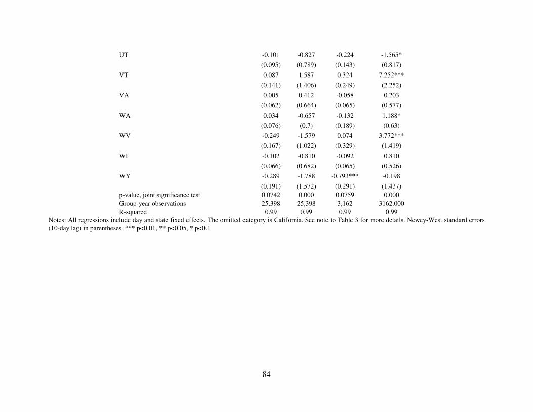
84

UT -0.101 -0.827 -0.224 -1.565*

(0.095) (0.789) (0.143) (0.817)

VT 0.087 1.587 0.324 7.252***

(0.141) (1.406) (0.249) (2.252)

VA 0.005 0.412 -0.058 0.203

(0.062) (0.664) (0.065) (0.577)

WA 0.034 -0.657 -0.132 1.188*

(0.076) (0.7) (0.189) (0.63)

WV -0.249 -1.579 0.074 3.772***

(0.167) (1.022) (0.329) (1.419)

WI -0.102 -0.810 -0.092 0.810

(0.066) (0.682) (0.065) (0.526)

WY -0.289 -1.788 -0.793*** -0.198

(0.191) (1.572) (0.291) (1.437)

p-value, joint significance test 0.0742 0.000 0.0759 0.000

Group-year observations 25,398 25,398 3,162 3162.000

R-squared 0.99 0.99 0.99 0.99

Notes: All regressions include day and state fixed effects. The omitted category is California. See note to Table 3 for more details. Newey-West standard errors (10-day lag) in parentheses. *** p<0.01, ** p<0.05, * p<0.1

85

Table A.13. Heterogeneity by 2007 House Price Growth in Sales Response to Market Tumult

Dependent variable: log 1099-B sales volume, USD Reported coefficient: interaction between change in log VIX and dummy for percentile of 2007 ZIP

code level house price growth

Sample Period

2008-2009 September - November

2008

Number of 1-day lagged differences: 1 10 1 10

(1) (2) (3) (4)

[80, 100] -0.053 -0.451 0.044 1.693***

(0.044) (0.410) (0.072) (0.285)

[60, 80) -0.049 -0.381 0.098** 1.267***

(0.037) (0.294) (0.049) (0.251)

[40, 60) -0.097*** -0.330 -0.015 1.266***

(0.034) (0.251) (0.046) (0.230)

[20, 40) -0.043 0.119 0.037 1.791***

(0.043) (0.386) (0.070) (0.249)

Group-day observations 2,490 2,490 310 310

R-squared 0.97 0.97 0.98 0.98

Notes: All regressions include day and group fixed effects. Omitted category is [0, 20). See note to Table 3 for more details. Newey-West standard errors (10-day lag) in parentheses. *** p<0.01, ** p<0.05, * p<0.1